The Use of Equalization Filters to Achieve

High Common Mode Rejection Ratios in

Biopotential Amplifier Arrays by

Hongfang Xia

A Thesis

Submitted to the Faculty

of

WORCESTER POLYTECHNIC INSTITUTE

in partial fulfillment of the requirements for the

Degree of Master of Science

in

Electrical and Computer Engineering

January 2005

APPROVED:

Professor Edward A. Clancy, Thesis Advisor Professor Donald R. Brown, Committee Member

Professor Brian M. King, Committee Member

i

ACKNOWLEDGEMENTS

I would like to acknowledge my indebtedness to my advisor Professor Edward A. Clancy

for his generous help and encouragement. I owed a lot to him, not just my engineering

skills and knowledge. Without his support, I cannot finish my thesis and make these

achievements with my research.

I am also thankful to Professor Brown for his helpful suggestions during my graduate

study and his presence in the committee. I am also thankful to Professor Brian M. King

for his presence in the committee, and all my friends, especially those in C(SP)2 lab,

including Mark, Karthik and Oli, who have gave me a lot of help in many ways.

I think I cannot give enough thanks to my dear family, especially my parents and my

husband.

ii

ABSTRACT

Recently, it became possible to detect single motor units (MUs) noninvasively via

the use of spatial filtering electrode arrays. With these arrays, weighted combinations of

monopolar electrode signals recorded from the skin surface provide spatial selectivity of

the underlying electrical activity. Common spatial filters include the bipolar electrode,

the longitude double differentiating (LDD) filter and the normal double differentiating

(NDD) filter. In general, the spatial filtering is implemented in hardware and the

performance of the spatial filtering apparatus is measured by its common mode rejection

ratio (CMRR). High precision hardware differential amplifiers are used to perform the

channel weighting in order to achieve high CMRR. But, this hardware is expensive and

all channel weightings must be predetermined. Hence, only a few spatially filtered

channels are typically derived.

In this project, a distinct software equalization filter was cascaded with each of the

hardware monopolar signal conditioning circuits to achieve accurate weighting and high

CMRR. The simplest technique we explored was to design an equalization filter by

dividing the frequency response of a “reference” (or “ideal”) channel by the measured

frequency response of the channel being equalized, producing the desired equalization

filter in the frequency domain (conventional technique). Simulation and experimental

results showed that the conventional technique is very sensitive to broadband background

noise, producing poor CMRR. Thus, a technique for signal denoising that is based on

signal mixing was pursued and evaluated both in simulation and laboratory experiments.

The purpose of the mixing technique is to eliminate the noise as much as possible prior to

equalization filter design. The simulation results show that without software equalization,

iii

CMRR is only around 30 dB; with conventional technique CMRR is around 50~60 dB.

By using mixing technique, CMRR can be around 70~80 dB.

iv

TABLE OF CONTENTS

ACKNOWLEDGEMENTS............................................................................................- 1 -

ABSTRACT....................................................................................................................- 2 -

TABLE OF CONTENTS................................................................................................- 4 -

LIST OF TABLES..........................................................................................................- 6 -

LIST OF FIGURES ........................................................................................................- 7 -

CHAPTER 1 INTRODUCTION ..............................................................................- 1 -

1.1 Project Objectives .........................................................................................- 1 -

1.2 Thesis Outline ...............................................................................................- 2 -

CHAPTER 2 BACKGROUND ................................................................................- 4 -

2.1 EMG Introduction.........................................................................................- 4 -

2.2 Standard EMG Array Detection System.......................................................- 6 -

2.3 Common Mode Rejection Ratio (CMRR) ..................................................- 13 -

2.3.1 Definition ..............................................................................................- 13 -

2.3.2 Measurement of CMRR........................................................................- 14 -

CHAPTER 3 Simulation of Equalization Filters ....................................................- 17 -

3.1 Conventional technique ..............................................................................- 20 -

3.1.1 Equalization Filter Frequency Response ..............................................- 20 -

3.1.2 CMRR Measurement ............................................................................- 22 -

3.1.3 Simulation Results For The Conventional Technique ..........................- 26 -

3.2 Mixing Technique.......................................................................................- 30 -

3.2.1 Mixing Algorithm .................................................................................- 31 -

3.2.2 System Configuration ...........................................................................- 35 -

v

3.2.3 CMRR Measurement ............................................................................- 36 -

3.2.4 Simulation Results Using Mixing Technique .......................................- 45 -

CHAPTER 4 LABORATORY EXPERIMENTS...................................................- 48 -

4.1 Hardware Introduction ................................................................................- 48 -

4.2 Experiment Results .....................................................................................- 54 -

4.2.1 Equalization Filter Response ................................................................- 54 -

4.2.2 CMRR Results ......................................................................................- 55 -

CHAPTER 5 PRELIMINARY RESULTS From A 28-CHANNEL ELECTRODE

ARRAY - 56 -

5.1 EMG hardware system................................................................................- 56 -

5.1.1 The EMG Array ....................................................................................- 56 -

5.1.2 Signal Conditional Circuits...................................................................- 58 -

5.2 Experiment Results .....................................................................................- 58 -

CHAPTER 6 CONCLUSIONS AND FUTURE WORK .......................................- 61 -

6.1 Discussion...................................................................................................- 61 -

6.2 Future Work ................................................................................................- 62 -

REFERENCES .............................................................................................................- 64 -

APPENDIX Signal Conditioning Circuit Schematics ...................................- 67 -

vi

LIST OF TABLES

Table 4-1 Measured Noise standard deviation (in µv) .................................................- 49 -

vii

LIST OF FIGURES

Figure 2-1 Schematic representation of the generation of ..............................................- 5 -

Figure 2-2 Standard EMG recording system ..................................................................- 6 -

Figure 2-3 Needle electrode [Neuman] ..........................................................................- 7 -

Figure 2-4 Wire electrode [Neuman]..............................................................................- 8 -

Figure 2-5 MUs located close to the skin surface (1) produce a spatially steep.............- 9 -

Figure 2-6 A schematic of the differential amplifier configuration [DeLuca02] .........- 10 -

Figure 2-7 LDD filter of pin electrodes placed on the skin [Reucher87].....................- 11 -

Figure 2-8 Four different EMG leads recording [Rau97] ............................................- 12 -

Figure 2-9 Signal conditioner diagram .........................................................................- 13 -

Figure 2-10 Differential amplifier with input sources [Hambley]................................- 14 -

Figure 2-11 Measurement of differential gain ..............................................................- 15 -

Figure 2-12 Measurement of common-mode gain........................................................- 15 -

Figure 3-1 System schematic configuration [Clancy01] ..............................................- 17 -

Figure 3-2 The flow chart of equalization filter design ................................................- 19 -

Figure 3-3 calibration data simulation model ...............................................................- 21 -

Figure 3-4 simulation model of CMRR measurement..................................................- 22 -

Figure 3-5 CMRR measurement configuration ............................................................- 25 -

Figure 3-6 Equalized channel outputs (absent noise) ...................................................- 27 -

Figure 3-7 Equalized channel outputs (1% noise) ........................................................- 28 -

Figure 3-8 Equalized channel outputs (3% noise) ........................................................- 29 -

Figure 3-9 CMRR vs noise level ..................................................................................- 30 -

viii

Figure 3-10 Mixer system configuration ......................................................................- 33 -

Figure 3-11 Equalization filter design model using mixing technique.........................- 35 -

Figure 3-12 CMRR measurement model......................................................................- 36 -

Figure 3-13 PSD plots for different CMRR (a) low CMRR, 40 dB, (b) high CMRR, 60

dB..................................................................................................................................- 37 -

Figure 3-14 CMRR measurement model......................................................................- 38 -

Figure 3-15 The mean and standard deviation of the error between the estimate and ideal -

40 -

Figure 3-16 The mean and standard deviation of the error of the estimate ..................- 40 -

Figure 3-17 The noise generated by two different amplifiers: TL084 and AD620 ......- 42 -

Figure 3-18 CMRR measurement configuration ..........................................................- 43 -

Figure 3-19 Estimated CMRR and true CMRR............................................................- 44 -

Figure 3-20 CMRR using linear shift technique...........................................................- 46 -

Figure 3-21 CMRR using windowing technique ..........................................................- 47 -

Figure 4-1 Recording processing model .......................................................................- 50 -

Figure 4-2 Calibration data ...........................................................................................- 51 -

Figure 4-3 Calibration data after carving out the buffer ...............................................- 52 -

Figure 4-4 Configuration for equalization filter design................................................- 52 -

Figure 4-5 Magnitude response of the equalization filter.............................................- 55 -

Figure 5-1 The schematic of one side of the array PCB board.....................................- 57 -

Figure 5-2 The electrode array......................................................................................- 57 -

Figure 5-3 28 channels EMG signal review .................................................................- 59 -

Figure 5-4 Equalized EMG signal (Bipolar) Right side is the zoomed view ...............- 59 -

ix

Figure 5-5 Equalized EMG signal (NDD) Lower is the zoomed view.........................- 59 -

Figure 5-6 EMG signal (NDD) before equalized .........................................................- 60 -

Figure 5-7 EMG signal (NDD) after equalized ............................................................- 60 -

1

CHAPTER 1 INTRODUCTION

1.1 Project Objectives

In recent years, surface electrode arrays have been developed to monitor the activity

of motor units (MUs) — the smallest controllable portion of a skeletal muscle. There is

an increasing interest in detecting single MU activity. Since it is hard to separate the

activity of a single MU from the simultaneously active adjacent ones, the method of

spatial filtering is used [Reucher86]. A spatial filtering is the weighted sum of several

electrode recordings (or detection sites). Typically, spatial filtering is preformed in

hardware. The accuracy of the weighting is measured in terms of common mode rejection

ratio (CMRR). Ideally, the CMRR is infinite, but because of nonlinear characteristics and

because components can never be exactly matched, typical CMRRs range from 60 to 120

dB at the fundamental power line frequency [Webster83].

With a hardware implementation, each different combination of detection sites

requires a distinct hardware channel to apply precise weights. In such systems, the

number of possibly useful derived signals can be too large for practical precision

implementation in hardware. Since it is impossible to match the hardware characteristics

of the distinct analog hardware channels, the number of electrode montages is limited for

research. The objective of this project is to achieve high CMRR and flexible electrode

combination via the use of software channel equalization. Similar equalization filters

have been used in applications such as communication systems and radar.

As will be presented later, a bench-top prototype electrode array system with 5

channels and a printed circuit board prototype electrode array system with 28 channels

2

have been developed. Each channel in each array is designed with an identical analog

signal conditioning circuit. Because of the component tolerances, the electrical

characteristics for each hardware channel are necessarily different. These characteristics

have been carefully measured to design the equalization filters. A distinct software

equalization filter is cascaded with each hardware channel to correct for the channel

difference. The software equalization filter is designed in the frequency domain. As will

be shown in chapter 3, the issue with a conventional equalization technique is that it is

very sensitive to noise. In this report, a new equalization design technique, termed our

“mixing technique,” has been evaluated to achieve high CMRR.

1.2 Thesis Outline

The rest of thesis is organized as follows:

Chapter 2 provides some background information about the electromyogram (EMG)

and its detection. This chapter focuses on the standard EMG detection system.

Additionally, this chapter gives some details regarding existing high resolution spatial

filters, the operating principle of spatial filters and their limitations in achieving high

CMRR in hardware.

Chapter 3 gives the system model of the software channel equalization procedure.

Section 3.1 explains the simple conventional technique to implement the equalization

filter and provides simulation results to explain why it is necessary to find an improved

technique. Section 3.2 gives the details of the new equalization filter implementation

technique – the mixing technique used in the thesis – including the mixing algorithm, the

low pass filter used in the system and the model for measuring CMRR.

3

Chapter 4 describes laboratory evaluation of the mixing technique using a five-

channel prototype array system. Signal test sources are generated from a signal generator,

passed through the analog signal conditioning circuits, and recorded using an A/D

converter.

Chapter 5 introduces the 28-channel electrode array hardware system that is used to

record the surface EMG signal from human subjects, including its hardware testing.

Moreover, the chapter provides pilot experiment results of performing equalization on

this array via the mixing technique.

Chapter 6 concludes the thesis with a discussion and summary. Some other possible

methods to implement the equalization filters are described.

4

CHAPTER 2 BACKGROUND

This chapter provides fundamental information about EMG signals and the standard

EMG detection systems. Additionally, different combinations of spatial filtering are

introduced as well as the concept of CMRR measurement

2.1 EMG Introduction

In a skeletal muscle, a motor unit (MU) is the smallest functional unit, consisting of

a single motor nerve and several muscle fibers. Under normal conditions, an action

potential propagating down a motor neuron activates all the branches of the motor neuron

[DeLuca79]; this action results in activating all the muscle fibers in that MU. When the

postsynaptic membrane of a muscle fiber is depolarized, the depolarization propagates in

both directions along the fiber; an electromagnetic wave is generated in the vicinity of the

muscle fibers by the membrane propagation [DeLuca79]. An electrode located in this

field can be used to detect the potential. This signal is called the electromyogram (EMG).

Figure 2-1 models how the motor unit action potential (MUAP) is generated and recorded

by electrode apparatus. The recorded EMG represents the superposition of MUs

generated by each of the myofibrils. For standard surface recording of the EMG signal,

its amplitude can range from 0 to 10 mV (peak to peak) or 0 to 1.5 mV RMS and most of

the energy of the signal is limited from DC to 500 Hz with the dominant energy in the

range of 15-150 Hz [DeLuca02].

5

Figure 2-1 Schematic representation of the generation of

the motor unit action potential [DeLuca79]

To detect single MU activity, high spatial resolution is required, because single MU

activity has to be separated from the simultaneous activity of adjacent MUs

[Disselhort98]. There are different approaches to detect the single MU activity. The most

common approach is using a needle or a wire electrode. With this technique, the

electrodes can be inserted into the muscle close to the desired location. Because of the

short distance between the MUs and the small size of the electrode, a needle/wire

electrode has high spatial resolution and single MU activity can be detected [Stalberg80].

But the insertion causes discomfort and creates the risk of infection [Disselhort98].

Additionally, the conventional needle/wire EMG techniques gain no information about

the excitation spread across a muscle and long time monitoring is not possible

6

[Disselhort98]. Moreover, the inserted needle/wire disturbs the electrical field which is

generated by the MU.

For these reasons, the detection of the single MU activity at the skin surface

becomes increasingly attractive. The conductive electrode which is used to detect the

surface EMG is much larger than the needle electrode and can be placed a long distance

away from the desired sites, but this causes the conventional surface EMG signal to be a

superposition of a large number of MUs [Rau97]. So, the conventional surface EMG has

a limited spatial selectivity.

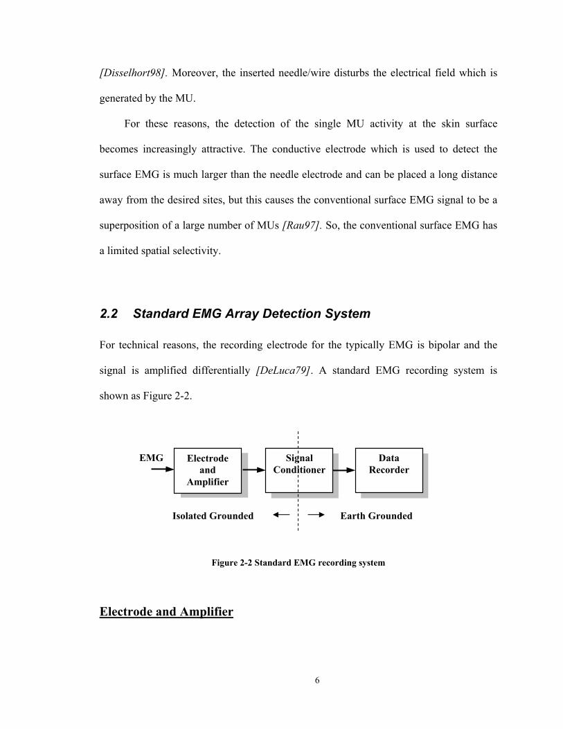
2.2 Standard EMG Array Detection System

For technical reasons, the recording electrode for the typically EMG is bipolar and the

signal is amplified differentially [DeLuca79]. A standard EMG recording system is

shown as Figure 2-2.

Figure 2-2 Standard EMG recording system

Electrode and Amplifier

Electrode and

Amplifier

Signal Conditioner

Data Recorder

EMG

Isolated Grounded Earth Grounded

7

In general, conductive electrodes are used to detect EMG. They can be either a

surface electrode, which is located on the skin surface overlying the muscle, or an

indwelling electrode, which is inserted into the muscle. There are two kinds of indwelling

electrodes: needle and wire.

Needle electrodes are used to penetrate the skin and tissue to reach the desired sites.

As stated above, the advantage of using needle electrodes is that, due to the short distance

between the MU and the recording sites, the spatial resolution is high enough to detect

the single MU activity [Disselhort98]. It also can be repositioned within the muscle. The

disadvantage of this technique is the discomfort and risk of infection because of the

insertion. Figure 2-3 shows typical needle electrodes.

Lead Wire

Hub

Insulating coating

Sharping metallic point

Coaxial lead wire

Hypodermic needle

Central electrode Insulation

(b) (c)

Figure 2-3 Needle electrode [Neuman]

Wire electrodes are smaller than needle electrodes. A hypodermic needle is used to

hold the wire electrode and insert it through the skin into the muscle at the desired site.

The advantage of using a wire electrode is that it can access deep musculature and detect

the single MU activity with little cross-talk (the absence of cross-talk means that the

signal sources close to the electrode will dominate the recorded EMG signal [Scott])

8

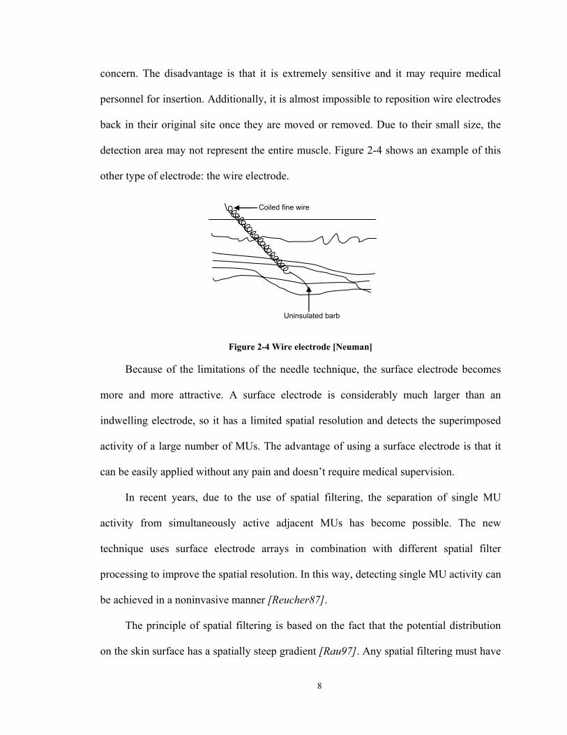
concern. The disadvantage is that it is extremely sensitive and it may require medical

personnel for insertion. Additionally, it is almost impossible to reposition wire electrodes

back in their original site once they are moved or removed. Due to their small size, the

detection area may not represent the entire muscle. Figure 2-4 shows an example of this

other type of electrode: the wire electrode.

Coiled fine wire

Uninsulated barb

Figure 2-4 Wire electrode [Neuman]

Because of the limitations of the needle technique, the surface electrode becomes

more and more attractive. A surface electrode is considerably much larger than an

indwelling electrode, so it has a limited spatial resolution and detects the superimposed

activity of a large number of MUs. The advantage of using a surface electrode is that it

can be easily applied without any pain and doesn’t require medical supervision.

In recent years, due to the use of spatial filtering, the separation of single MU

activity from simultaneously active adjacent MUs has become possible. The new

technique uses surface electrode arrays in combination with different spatial filter

processing to improve the spatial resolution. In this way, detecting single MU activity can

be achieved in a noninvasive manner [Reucher87].

The principle of spatial filtering is based on the fact that the potential distribution

on the skin surface has a spatially steep gradient [Rau97]. Any spatial filtering must have

9

an inverting and a noninverting part, and the sum of the channel weights must equal zero

to eliminate the powerline interference. Figure 2-5 shows the potential contributed by

MUs located close to the skin surface. It shows a bipolar lead with small sized electrodes

separated by a few millimeters and arranged parallel to the muscle fibers. It forms the

lowest order spatial filter — the bipolar configuration — which differentiates the

potential distribution in the direction of the electrode configuration. The operation of the

bipolar filter is very simple. It differentiates the potential distribution generated on the

skin surface, and then amplifies the difference. Thus, it is also called a pre-amplifier. A

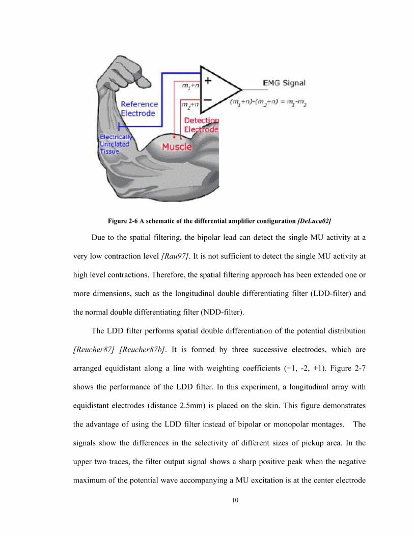
schematic of this configuration is shown as Figure 2-6. The EMG signal is represented as

“m” and the common interference signal is represented as “n”.

Figure 2-5 MUs located close to the skin surface (1) produce a spatially steep

potential gradient (A) in the recording area; (2) a flat potential course. Using a

bipolar lead with a small interelectrode distance the flat potential course

contributes only with a small part (∆U2) to the measured total value (∆U) [Rau97]

10

Figure 2-6 A schematic of the differential amplifier configuration [DeLuca02]

Due to the spatial filtering, the bipolar lead can detect the single MU activity at a

very low contraction level [Rau97]. It is not sufficient to detect the single MU activity at

high level contractions. Therefore, the spatial filtering approach has been extended one or

more dimensions, such as the longitudinal double differentiating filter (LDD-filter) and

the normal double differentiating filter (NDD-filter).

The LDD filter performs spatial double differentiation of the potential distribution

[Reucher87] [Reucher87b]. It is formed by three successive electrodes, which are

arranged equidistant along a line with weighting coefficients (+1, -2, +1). Figure 2-7

shows the performance of the LDD filter. In this experiment, a longitudinal array with

equidistant electrodes (distance 2.5mm) is placed on the skin. This figure demonstrates

the advantage of using the LDD filter instead of bipolar or monopolar montages. The

signals show the differences in the selectivity of different sizes of pickup area. In the

upper two traces, the filter output signal shows a sharp positive peak when the negative

maximum of the potential wave accompanying a MU excitation is at the center electrode

11

at the LDD filter [Reucher87]. In spite of the high contraction level, the impulses of four

different MU’s (labeled A, B, C and D in the figure) can be distinguished by their

amplitude and their direction of propagation [Reucher87]. In the lower two traces, single

MU’s cannot be separated because many MU’s are simultaneously discharging. This

figure shows the advantages of recording with selective spatial filters.

Figure 2-7 LDD filter of pin electrodes placed on the skin [Reucher87]

The NDD filter (a.k.a. a Laplace filer) is well suited for the detection of edges

perpendicular to the direction of the differentiation [Disselhorst97]. It is formed by a

weighted summation of five crosswise-arranged electrodes. The weighting factors of each

electrode are represented by the filter mask [Disselhorst97]

−=

010141010

NDDM .

The rows and the columns of the filter mask are identical to the rows and columns of the

electrode array.

12

Figure 2-8 compares the performance for four different EMG spatial filters using

data recorded from the m. abductor pollicis brevis muscle at maximum voluntary

contraction. It shows that the bipolar electrode does not sufficiently distinguish individual

MU activity at high contraction level but the NDD can separate the single MU activity.

As the spatial filtering extended to three or more electrodes, the spatial selectivity

improved. The NDD filter improves the spatial selectivity in all directions and can detect

single MU activity even at maximum voluntary contraction.

Figure 2-8 Four different EMG leads recording [Rau97]

Signal Conditioner

Figure 2-9 shows a system-level diagram of a signal conditioner. In general, the

signal conditioner consists of a high pass filter, which attenuates motion artifact and any

offset potentials; selectable gain, which magnifies the signal up to the range of the data

recording/monitoring instrumentation; electrical isolation, which prevents injurious

13

current from entering the patient; and a low pass filter, which prevents anti-aliasing and

attenuates noise out of the physiologic frequency range.

Figure 2-9 Signal conditioner diagram

2.3 Common Mode Rejection Ratio (CMRR)

2.3.1 Definition

CMRR is defined as the ratio of the magnitude of the differential gain to the

magnitude of the common mode gain of two channels. Often, CMRR is expressed in dB

as

)(log20 10c

d

GG

CMRR = Equation 2-1

where dG is the magnitude of the differential signal and cG is the magnitude of the

common signal. Ideally, the CMRR is infinite, but for the existing equipment, because of

nonlinear characteristics and because components can never be exactly matched, typical

CMRRs range from 60 to 120 dB at the fundamental power line frequency [Webster83].

High Pass Filter

Selectable gain

Electrical Isolation

Low Pass Filter

14

2.3.2 Measurement of CMRR

Differential Amplifier [Hambley]

For two input signals, an ideal differential amplifier is shown in Figure 2-10.

Figure 2-10 Differential amplifier with input sources [Hambley]

The difference between the input voltages is amplified by gain Gd, giving the output

voltage (Vo) as:

( ) 2121 ididiido vGvGvvGv −=−= Equation 2-2

The difference between the input voltages Vi1 and Vi2 is known as the differential

signal idv .

21 iiid vvv −= Equation 2-3

We refer to the gain dG as the differential gain. So, the output of the ideal differential

amplifier can be written as

iddo vGv = Equation 2-4

The input sources 1iv and 2iv can be replaced by the equivalent sources icmv and idv ,

where icmv is the common mode signal and is given by

15

( )2121

iiicm vvv += Equation 2-5

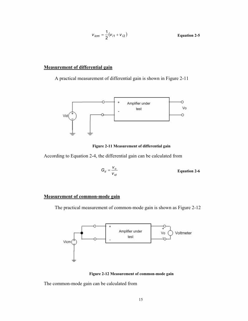
Measurement of differential gain

A practical measurement of differential gain is shown in Figure 2-11

Figure 2-11 Measurement of differential gain

According to Equation 2-4, the differential gain can be calculated from

id

od v

vG = Equation 2-6

Measurement of common-mode gain

The practical measurement of common-mode gain is shown as Figure 2-12

Figure 2-12 Measurement of common-mode gain

The common-mode gain can be calculated from

16

icm

oc v

vG = Equation 2-7

where icmv can be calculated from Equation 2-5.

The higher the CMRR, the better the performance of the subtraction process within

the amplifier. For bipolar electrodes, CMRR is the ratio of the common-mode

interference voltage at the input of a circuit, to the corresponding interference voltage at

the output. As shown in Figure 2-6, the signals are detected at two sites, subtracted by the

differential amplifier and gain amplified. With this operation, any signal that is

“common” to both sites will be removed and any signal that is different will be amplified.

Thus, relatively distant power line interference signals (which appear as common signals

at each electrode) will be removed and relatively local EMG signals will be amplified

[DeLuca02]. In practice, it is very difficult to remove the common signal perfectly. In

general, the subtraction is performed in hardware. Currently, we can achieve CMRRs as

high as 120 dB with hardware. But there are limitations with hardware implementations,

such as high expense, the requirement to build a separate circuit for each spatial channel

desired, and that power line interference does not present an exactly common signal to

each electrode site.

17

CHAPTER 3 Simulation of Equalization Filters

The purpose of this project is to implement equalization filters in software to

achieve high CMRR. Figure 3-1 shows the general system configuration. For the

hardware system, a 5-channel bench-top prototype and a 4x7 equal-spaced rectangular

array prototype have both been developed. For both, each channel is designed with an

identical analog circuit design. All of the resistors have 1% tolerance and the capacitors

have 5% tolerance. A distinct software equalization filter is cascaded with each signal

conditioner circuit.

Figure 3-1 System schematic configuration [Clancy01]

In general, the equalization filter is determined by measuring the frequency-

dependent gain and phase of each analog signal conditioning channel. The desired

(“ideal”) frequency response divided by the measured frequency response gives the

frequency response of the equalization filter. After the frequency response of the

Analog Signal Conditioning Circuit

#1

Analog Signal Conditioning Circuit

#2

Analog Signal Conditioning Circuit

#N

e1

e2

eN

Ele

ctro

de In

puts

A/D Linear Equalization

Filter #1 EMG1

A/D Linear Equalization

Filter #2 EMG2

A/D Linear Equalization

Filter #N EMGN

Equalized C

hannels

Hardware Software

18

equalization filter eH is achieved, a FIR filter with order 12 +L is designed (to be used to

implement the filter in the time domain).

Note that the impulse response of the equalization filter, using the transfer function

approach, must be real-valued. To prove this assertion, begin by assuming that the output

of the reference channel is ( )tx and the output of the equalized channel is ( )ty . By using

the transfer function approach, the frequency response of the equalization filter ( )wH can

be written as in Equation 3-1.

( ) ( )( )wXwYwH = Equation 3-1

Notice that both ( )ty and ( )tx are real signals. For real signal ( )tx , its transform must be

of the form

( ) ( ) ( )wjXwXwX IR += Equation 3-2

where ( ) ( )∑∞

−∞==n

R wnnxwX cos and ( ) ( )∑∞

−∞==n

I wnnxwX sin [Proakis96, P287]. It follows that

( ) ( )( ) ( )wXwX

wXwX

II

RR

−=−

=−

Similarly with the reference channel,

( ) ( )( ) ( )wYwY

wYwY

II

RR

−=−

=−

The transform

( ) ( ) ( ) ( )( )

( ) ( )( ) ( )( ) ( ) ( ) ( )

( ) ( )( ) ( ) ( ) ( )

( ) ( )wXwXwXwYwXwYj

wXwXwXwYwXwY

wjXwXwjYwY

wXwYwjHwHwH

IR

RIIR

IR

IIRR

IR

IR

IR

2222 +−

+++

=

++

=

=+=

So, we get that

19

( ) ( ) ( ) ( ) ( )( ) ( )

( ) ( ) ( ) ( ) ( )( ) ( )wXwX

wXwYwXwYwH

wXwXwXwYwXwY

wH

IR

RIIRI

IR

IIRRR

22

22

+−

=

++

=

,

( ) ( ) ( ) ( ) ( )( ) ( )

( ) ( ) ( )[ ] ( )[ ]( ) ( )

( ) ( ) ( ) ( )( ) ( )

( )wHwXwX

wXwYwXwYwXwX

wXwYwXwYwXwX

wXwYwXwYwH

R

IR

IIRR

IR

IIRR

IR

IIRRR

=++

=

+−−+

=

−+−−−+−−

=−

22

22

22

, and

( ) ( ) ( ) ( ) ( )( ) ( )

( ) ( ) ( ) ( )( ) ( )

( )wHwXwX

wXwYwXwYwXwX

wXwYwXwYwH

I

IR

RIIR

IR

RIIRI

−=++−

=

−+−−−−−−

=−

22

22

Thus, we can say that the impulse response ( )nhe of the equalization filter must be real.

In this report, two filter design methods will be introduced to form the FIR filter

based on the frequency response. The first method is the windowing technique. Figure

3-2 shows the diagram of this method.

Figure 3-2 The flow chart of equalization filter design

In general, the coefficients of the (2L+1)th order FIR filter can be obtained by truncating

the sequence ( )nhe at point 12 +L . Truncation of ( )nhe to a length 12 +L is equivalent to

using a “rectangular window” [Proakis96]. Other window functions can also be used in

this stage such as a “hamming window” or “hanning window”. Thus, the time-domain

filter, b(n) can be formed as

eH IFFT Truncate by 12 +L

20

( ) 12,,2,1 +=⊂ Lnnhb en K Equation 3-3

The second method consists of implementing a linear shift (advance) of the input

sequence by half the FIR filter order before the frequency response of the equalization

filter is calculated. The reason for this shift is that the signals propagating through a

physical hardware channel can either lag or lead the phase of a signal propagating

through an ideal channel. Without this linear shift, significant power can result at the end

of the impulse response (due to the frequency response representing a non-causal signal

propagation), but will be discarded with the simple windowing technique. Later, we will

show the results using these two equalization filter designs.

3.1 Conventional technique

To determine the frequency response of the equalization filter using our

“conventional” technique, the desired (“ideal”) frequency response is divided by the

measured frequency response. In this section, we will illustrate the simulation results for

this conventional technique and show that this technique is not sufficient to achieve high

CMRR. Also, we will present the new technique – a mixing technique – comparing these

two techniques. First, we will introduce the conventional technique.

3.1.1 Equalization Filter Frequency Response

21

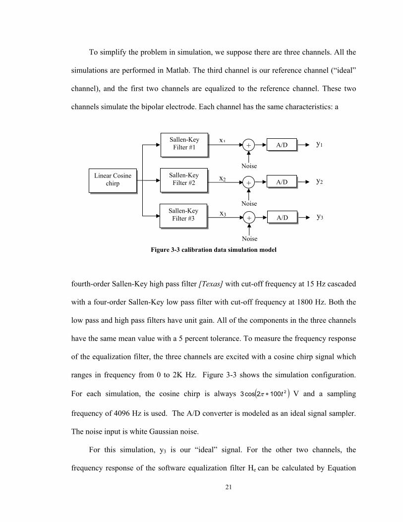
To simplify the problem in simulation, we suppose there are three channels. All the

simulations are performed in Matlab. The third channel is our reference channel (“ideal”

channel), and the first two channels are equalized to the reference channel. These two

channels simulate the bipolar electrode. Each channel has the same characteristics: a

Figure 3-3 calibration data simulation model

fourth-order Sallen-Key high pass filter [Texas] with cut-off frequency at 15 Hz cascaded

with a four-order Sallen-Key low pass filter with cut-off frequency at 1800 Hz. Both the

low pass and high pass filters have unit gain. All of the components in the three channels

have the same mean value with a 5 percent tolerance. To measure the frequency response

of the equalization filter, the three channels are excited with a cosine chirp signal which

ranges in frequency from 0 to 2K Hz. Figure 3-3 shows the simulation configuration.

For each simulation, the cosine chirp is always ( )21002cos3 t∗π V and a sampling

frequency of 4096 Hz is used. The A/D converter is modeled as an ideal signal sampler.

The noise input is white Gaussian noise.

For this simulation, y3 is our “ideal” signal. For the other two channels, the

frequency response of the software equalization filter He can be calculated by Equation

Linear Cosine chirp

Sallen-Key Filter #1

Sallen-Key Filter #2

Sallen-Key Filter #3

+

Noise

x1

+

Noise

x2

+

Noise

x3

y1 A/D

y2 A/D

y3 A/D

22

3-4, where i is the channel number. In this project, the length of the data sequence is

409600.

( ) ( )( )i

ie yfft

yfftH 3= Equation 3-4

3.1.2 CMRR Measurement

3.1.2.1 Equivalent CMRR Measurement

The CMRR measurement model in this report is shown in Figure 3-4

Figure 3-4 simulation model of CMRR measurement

Here we assume that,

Every channel is a linear system at frequency 0w .

Signal X ,Y , 'X and 'Y are voltage phasers.

Both xG and yG are complex number gains.

Note that our CMRR measurements are made at a fixed frequency.

Measurement of common-mode gain in simulation

We apply cV (voltage phaser, i.e., a sinusoid) to both channels X and Y . Thus the

common mode gain is

23

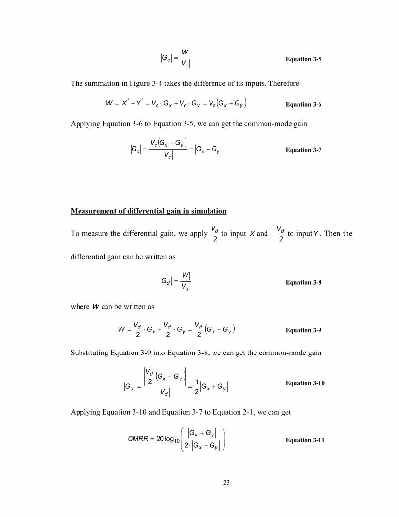
cc V

WG = Equation 3-5

The summation in Figure 3-4 takes the difference of its inputs. Therefore

( )yxcycxc GGVGVGVYXW −=⋅−⋅=−= '' Equation 3-6

Applying Equation 3-6 to Equation 3-5, we can get the common-mode gain

( )yx

c

yxcc GG

V

GGVG −=

−= Equation 3-7

Measurement of differential gain in simulation

To measure the differential gain, we apply 2dV to input X and

2dV− to inputY . Then the

differential gain can be written as

dd V

WG = Equation 3-8

where W can be written as

( )yxd

yd

xd GG

VG

VG

VW +=⋅+⋅=

222 Equation 3-9

Substituting Equation 3-9 into Equation 3-8, we can get the common-mode gain

( )yx

d

yxd

d GGV

GGV

G +=+

=212 Equation 3-10

Applying Equation 3-10 and Equation 3-7 to Equation 2-1, we can get

−⋅

+=

yx

yx

GG

GGCMRR

2log20 10 Equation 3-11

24

Because we use a single-ended amplifier in our simulation, if we apply a common signal

cV in,

cyyc

cxxc

VYGGVYVXGGVX

/''/''

=⇒⋅=

=⇒⋅= Equation 3-12

Substituting Equation 3-12 into Equation 3-11, we get

−⋅

+=

''2''

log20 10 YXYX

CMRR Equation 3-13

3.1.2.2 CMRR Measurement Model

After obtaining the coefficients of the equalization filter in the time domain for each

channel, we evaluated their performance by measuring the CMRR. Figure 3-5 shows the

CMRR measurement configuration. Since the dominant interference from the power lines

is at 60 Hz (or 50 Hz in some regions outside of North America) [DeLuca02], the CMRR

at 60 Hz is measured. In this simulation, we excite the first and second channel with a 60

Hz sine waveform, which then passes through the Sallen-Key filter and the equalization

filter. The signals ye1 and ye2 are the equalized channel outputs. With ideal equalization

(infinite CMRR), the signals would be zero-valued at all times (at least in the absence of

any noise). Using Equation 3-13, we can measure the CMRR.

25

Figure 3-5 CMRR measurement configuration

By using Equation 3-13, the CMRR between the two outputs 1ey and 2ey can be written

as

⋅=

c

d

AA

CMRR2

log20 10 Equation 3-14

where dA is the magnitude of the sum of the two output signals 1ey and 2ey at 60Hz and

cA is the magnitude of the difference between the two output signals at 60Hz. Define

( ) ( ) ( )tytyts ee 21 += and ( ) ( ) ( )tytytc ee 21 −= . In practice, for the sum of the two signals

( )ts , it is easy to measure its magnitude at 60 Hz. But, if the two signals are matched

precisely, it is hard to measure the magnitude of the difference of the signals ( )tc ,

particularly in the presence of noise.

One way to measure the amplitude of the signal ye1(t)-ye2(t) is via direct measure of

its power at 60 Hz from the power spectral density of the differential signal ( )tc . The

drawback of this technique is that in order to accurately measure the PSD at 60 Hz, the

noise level must be significantly lower than the signal level at this frequency. For

CMRRs above 40–50 dB, which means the difference between the two channels are

smaller, the noise is lager than the 60 Hz signal when we subtract the two channels.

60 Hz sine

Sallen-Key filter #1

Sallen-Key filter #2

bn(1)

bn(2)

ye1

ye2

+

A/D

Noise

Noise

A/D +

26

However, the power spectrum technique was sufficient for CMRR measurement for

conventional equalization.

3.1.3 Simulation Results For The Conventional Technique

In this section, we present the simulation results for the conventional equalization

technique. We will show that the main problem is its sensitivity to noise. In this

simulation, we will vary the noise level to see how the noise affects the performance of

the system.

Absent noise

In this simulation, we set the noise level to zero. After the frequency response of the

filter is measured, a FIR filter is designed using the simple windowing technique (i.e.,

absent the linear shift operation). Figure 3-6 shows the difference between the two

equalized channel outputs. From the previous discussion, the major issue that affects

CMRR is the background noise. Since the noise level is zero, the CMRR should be

infinite (ideally). There is no quantization noise in this simulation since an all pass filter

is used instead of a quantizer.

27

0 10 20 30 40 50 60 70 80 90 100-1

-0.8

-0.6

-0.4

-0.2

0

0.2

0.4

0.6

0.8

1Difference between channel II and channel I

Mag

nitu

de in

Vol

ts

Time in Seconds

Figure 3-6 Equalized channel outputs (absent noise)

1 percent noise

Next, we set the standard deviation of the background noise level to 1 percent of the

input signal amplitude. The resulting CMRR is around 40 dB. Plots showing this

simulation, following the format described above, are shown in Figure 3-7.

28

0 10 20 30 40 50 60 70 80 90 100-0.4

-0.3

-0.2

-0.1

0

0.1

0.2

0.3Difference between channel II and channel I

Mag

nitu

de in

Vol

ts

Time in Seconds

Figure 3-7 Equalized channel outputs (1% noise)

3 percent

Lastly, the noise standard deviation was increased to 3 percent of the input signal

amplitude. The resulting CMRR is around 25 dB. Plots showing this simulation,

following the format described above, are shown in Figure 3-8.

29

0 10 20 30 40 50 60 70 80 90 100-1

-0.8

-0.6

-0.4

-0.2

0

0.2

0.4

0.6

0.8Difference between channel II and channel I

Mag

nitu

de in

Vol

ts

Time in Seconds

Figure 3-8 Equalized channel outputs (3% noise)

30

0 0.5 1 1.5 2 2.5 30

50

100

150

200

250

noise level (percent)

CM

RR

in d

B

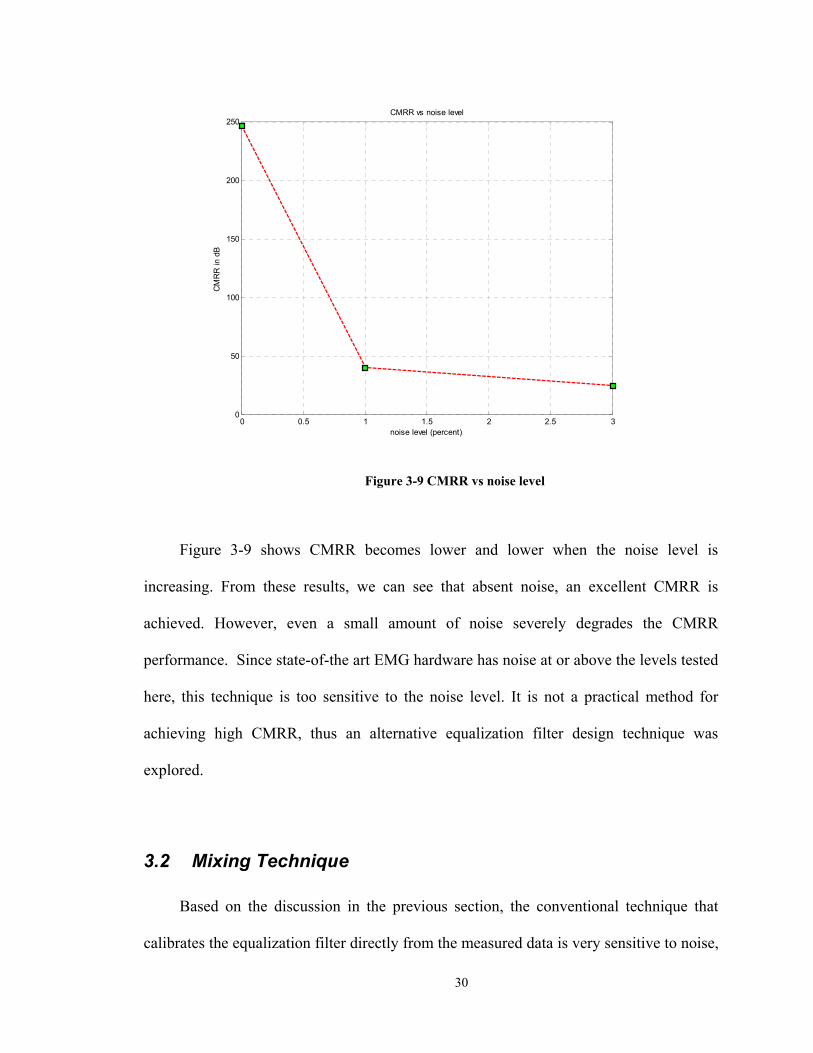
CMRR vs noise level

Figure 3-9 CMRR vs noise level

Figure 3-9 shows CMRR becomes lower and lower when the noise level is

increasing. From these results, we can see that absent noise, an excellent CMRR is

achieved. However, even a small amount of noise severely degrades the CMRR

performance. Since state-of-the art EMG hardware has noise at or above the levels tested

here, this technique is too sensitive to the noise level. It is not a practical method for

achieving high CMRR, thus an alternative equalization filter design technique was

explored.

3.2 Mixing Technique

Based on the discussion in the previous section, the conventional technique that

calibrates the equalization filter directly from the measured data is very sensitive to noise,

31

which results in low CMRR. It is necessary to find a new technique that is less sensitive

to the noise and can be easily implemented in software. As we have found, the major

impediment to achieving high CMRR is the broadband background noise which cannot

be eliminated within the hardware. Certainly, the hardware should eliminate as much

noise as possible. We focused on a signal processing method, based on a mixing

technique common in communications engineering, to remove noise from the signals.

3.2.1 Mixing Algorithm

In using this technique, we assume that the input signal is a linear chirp with a fixed

magnitude and sweeping rate. The premise of this technique is mixing the measured chirp

waveform with another chirp waveform that has the same sweep rate and initial

frequency. The resultant outputs will be the sum of two chirps – one with double the

sweep rate which can be filtered out by a proper low pass filter, and one with a zero

sweep rate (DC signal) which contains all the magnitude and phase information of the

measured chirp waveform. In this section, we will introduce the mixing algorithm and

how to choose the proper parameters for the mixer.

Chirp Presentation

A linear chirp can be written as

( )

= ++ θ2

0Re wttwjAechirplinear Equation 3-15

By using Euler's identity

[ ] ( )2

cosRejwtjwt

jwt eewte−+

==

32

the linear chirp can be re-written as

( ) ( )[ ]inin wttwjwttwj eeAchirplinear θθ ++−++ −=2

02

0

2 Equation 3-16

where 0w , w , θ are constants. The instantaneous angular frequency is

( )wtw

dtwttwd

w ininst 20

20 +=

++=

θ Equation 3-17

Let awbw ππ 2,20 == , where a (Hz/s), and b (Hz) are scaling constants. Hence the

linear chirp can also be written as

( ) ( )[ ]inin btatjbtatj eeAchirplinear θππθππ ++−++ −= 2222 22

2 Equation 3-18

and has an instantaneous frequency of

bat2f += Equation 3-19

For example, a ten-second linear chirp formed by selecting a = 100 and b = 0 would

begin at 0 Hz and end at 2 K Hz.

More generally, if such a chirp is passed through a linear system, the output ( )ts is

also a chirp, but can be modified in magnitude and phase at each frequency and

embedded in an independent additive noise. Let the input ( )tw to the linear system be

written as

( ) ( ) ( )[ ]inin btatjbtatjin eeA

tw θππθππ ++−++ −= 2222 22

2 Equation 3-20

Since the frequency of the input chirp has a direct (and known) relation to time, the

magnitude and phase distortion imposed by the linear system can be captured by the time

variant magnitude ( )tA and phase ( )tθ of the output, written as

33

( ) ( ) ( )( ) ( )( )[ ] ( )tneetAts tbtatjtbtatj +−= ++−++ θππθππ 2222 22

2Equation 3-21

where ( )tn is the additive noise, ( ) ( )in

outA

tAtA = is the magnitude distortion (a value of one

for a given time indicates no magnitude distortion, a value greater than one indicates that

the linear system amplifies the signal, and a value less than one indicates that the linear

system attenuates the signal) and ( ) ( ) inout tt θθθ −= is the phase modulation (a value of

zero radians for a given time indicates no phase distortion, a value greater than zero

indicates an induced phase lag).

Mixing Algorithm

Based on the previous discussion, the mixer configuration is shown in Figure 3-10,

Figure 3-10 Mixer system configuration

where the input signal ( ) ( ) ( ) ( )tneeA

tx inbtatjbtatjin inin +

−= ++−++ θππθππ 2222 22

2 , ( )wH is a

linear system and the mixer ( ) ( )mttjetm θπβπα ++−= 22 22 where α (Hz/s), and β (Hz) are

scaling constants.

Using Equation 3-21, the output ( )ts of the linear system is written as

( ) ( ) ( ) ( )( )[ ] ( )tneetA

ts outtbtatjbtatjout out +−= ++−++ θππθππ 2222 22

2

where ( )tnout is the noise signal after the noise ( )tnin passing through the linear system.

x(t) X

m(t)

H(w) ym(t) s(t) LPF sm(t)

34

When the mixer is applied to the linear system output, we produce

( ) ( ) ( )( ) ( )( ) ( )( )[ ] ( )( ) ( ) ( ) ( ) ( )( )[ ]

( ) ( ) ( ) ( )( )[ ]

( ) ( )m

mout

mout

m

outout

ttjout

ttbtajout

ttbtajout

ttj

outtbtatjtbtatjout

m

etn

etA

etA

e

tneetAtmtsty

θπβπα

θθβπαπ

θθβπαπ

θπβπα

θππθππ

++

−+−+−−

+++++

++

++−++

−

+

−=

−⋅

+−=

⋅=

22

22

22

22

2222

2

2

2

2

22

2

2

2 Equation 3-22

where ( )tym is the mixed output. This resultant signal can be thought of as the sum of

three signals — one with the sum sweep rate, one with the difference sweep rate and the

other one with the broadband noise. For the difference signal, the frequency variation

carries the magnitude and phase information as a function time. By selecting proper

values for the mixer, we can produce carrier frequencies at DC (for the difference signal)

and at double sweep rate (for the sum signal).

For example, by selecting ,a=α b=β , and 0=mθ we can get

( ) ( ) ( )[ ]( ) ( )[ ]

( ) ( )bttjout

tjout

tbtatjoutm

etn

etA

etAtyout

out

ππα

θ

θππ

22

2222

2

2

2 +

−

+⋅+⋅

−

+

−= Equation 3-23

By applying a low pass filter, the double rate signal can be eliminated, as well as most of

the noise (except for signal that entered during the start-up transient of the low pass filter).

Thus, if we ignore the start-up, the following output remains after filtering:

( ) ( ) ( )[ ]tjoutm

outetAts θ−= Equation 3-24

Now we can see that the magnitude of the output is the instantaneous magnitude of

the measured signal and the phase of the output is the instantaneous phase of the

measured signal. Then, we can extract the instantaneous magnitude and phase

information of the measured signal in the time domain.

35

( ) ( )( ) ( )tst

tstA

mout

mout

−∠=

=

θ Equation 3-25

3.2.2 System Configuration

The simulation processing for this technique also has two steps:

1. Generate the calibration signal to construct the equalization.

2. Measure the performance by calculating the CMRR at 60 Hz.

The simulation model for equalization filter design is show as Figure 3-11.

Figure 3-11 Equalization filter design model using mixing technique

To design the equalization filter, the most difficult issue is the design of the low-

pass filter (LPF) that resides after the mixer, since its cut-off frequency should be less

than 1% of the Nyquist frequency. At first, we attempted to design the LPF in the

frequency domain using the optimal nonrecursive digital filter presented by Rabiner in

1970 [Rabiner]. The performance of this filter was not sufficient. Thus, we resorted to a

filter designed using the windowing method which utilizes a large number (greater than

3000) of coefficients. The number of filter coefficients is limited by the start frequency

Linear Cosine chirp

Sallen-Key Filter #1

Sallen-Key Filter #2

Sallen-Key Filter #3

+

Noise

x1

+

Noise

x2

+

Noise

x3

y1 A/D X

m(t)

LPF s1

y2 A/D X

m(t)

LPF s2

y2 A/D X

m(t)

LPF s3

36

and sweep duration of the input chirp signal. The EMG signal contains most of its power

from 50-150Hz. Thus, the length of the LPF must be such that the input chirp, which

sweeps upwards from 0 Hz, is not distorted in the 50–150 Hz range due to the startup

transient of the filter.

3.2.3 CMRR Measurement

CMRR measurement with the mixing technique was logically the same as using the

conventional technique and is re-drawn as Figure 3-12. However, we previously noted

that CMRR measurement via the power spectrum is impractical for high CMRR

measurement. In order to measure the PSD of the common mode signal, the noise level in

the signal cannot be higher than the 60 Hz signal.

Figure 3-12 CMRR measurement model

Figure 3-13 shows the PSD plots for simulations resulting in low and high CMRRs.

The x-axis in this figure is normalized frequency. For the low CMRR case (40 dB), the

60 Hz signal is visible in the PSD plot. In this case, we can estimate the PSD for the

common mode signal. While for the high CMRR (90 dB), the 60 Hz signal is unclear

because the noise dominates the whole signal. By using the mixing technique, the

60Hz sine wave

Sallen-Key filter #1

Sallen-Key filter #2

bn(1)

bn(2)

ye1

ye2

+

A/D

Noise

Noise

A/D +

37

expected CMRR is higher than using the conventional technique, thus we cannot use the

same method to measure the CMRR. In this section, we describe a method for measuring

higher CMRRs and point out the limitation of this method.

0 0.2 0.4 0.6 0.8 1-41

-40.5

-40

-39.5

-39

-38.5

-38

-37.5

-37

Frequency

Pow

er S

pect

rum

Mag

nitu

de (d

B)

(a)

0 0.2 0.4 0.6 0.8 1-41

-40.8

-40.6

-40.4

-40.2

-40

-39.8

-39.6

-39.4

-39.2

Frequency

Pow

er S

pect

rum

Mag

nitu

de (d

B)

(b)

Figure 3-13 PSD plots for different CMRR (a) low CMRR, 40 dB, (b) high CMRR, 60 dB

The CMRR between the two outputs 1ey and 2ey can be calculated from Equation

3-14.

⋅=

c

d

AA

CMRR2

log20 10 Equation 3-14

where dA is the magnitude of the sum of the two signals and cA is the magnitude of the

difference between the two signals. Define ( ) ( ) ( )tytyts ee 21 += and ( ) ( ) ( )tytytd ee 21 −= .

In general, we can use the PSD estimation technique to measure the magnitude of ( )ts , as

the magnitude of this signal is well above the noise floor. To measure the magnitude

of ( )td , a new method was investigated in simulation.

38

NSR (noise – to - signal ratio)

We define NSR as a measure of signal strength relative to the background noise.

NSR is the ratio of the standard deviation Nσ of the noise to the magnitude sAmp of the

60 Hz signal, where the noise is white Gaussian noise.

s

N

AmpNSR

σ= Equation 3-26

From the definition of NSR, the magnitude cA of ( )td can be written as

NSRA Nc /σ= Equation 3-27

Substituting Equation 3-27 into Equation 3-14, we get

⋅=

N

dANSRCMRR

σ2log20 10 Equation 3-28

CMRR Measurement

The simulation model is shown in Figure 3-14.

Figure 3-14 CMRR measurement model

where ( )td is the incoming signal, ( )tn is additive white Gaussian noise and ( )tx is the

output of channel x. To simply this simulation, consider a 60Hz signal ( )td with large

additive white Gaussian noise ( )tn

( ) ( ) ( )tntdtx += Equation 3-29

39

We focus on the estimate of the magnitude of ( )td . Because the noise is white and

Gaussian, noise outside of the frequency region around 60 Hz can be attenuated via the

use of a notch filter. Letting signal ( )tx pass through this notch filter, most of the noise

will be eliminated. The output can be written as

( ) ( ) ( )tntdtx 11 += Equation 3-30

where ( )tn1 is the residual noise. To estimate the magnitude of ( )td , we use nonlinear

curve fitting to fit ( )tx1 into a 60 Hz signal ( )tdest = ( )estest tAmp θπ +∗ 602sin . The

magnitude estAmp of ( )tdest is the common signal amplitude.

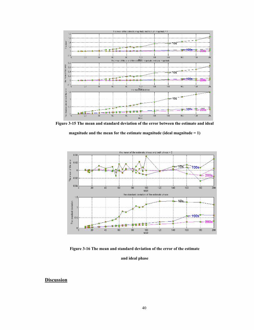
Here we show some simulation results. In this simulation, we evaluated 10 second,

100 second and 200 second signal durations. For each input signal, we let the 60 Hz input

have unit magnitude and we varied the noise to signal ratio (NSR ). We used this method

to measure the magnitude and phase of the input signal and compared the measured

results to the ideal values. We repeated every simulation scenario 1000 times to get 1000

results and computed the sample mean and sample standard deviation of these 1000

results. The results are shown in Figure 3-14 and Figure 3-15.

40

Figure 3-15 The mean and standard deviation of the error between the estimate and ideal

magnitude and the mean for the estimate magnitude (ideal magnitude = 1)

Figure 3-16 The mean and standard deviation of the error of the estimate

and ideal phase

Discussion

41

From the result of the experiments, we can see that for 100 second and 200 second

signal durations, even a NSR is large as 100 still resulted in an amplitude estimate with

acceptable error. From Equation 3-28

⋅=

N

dANSRCMRR

σ2log20 10 Equation 3-28

Letting 100=NSR and 01.02 == NdA σ , we can get

9.7302.022100log20 10 =

⋅⋅

=CMRR dB

Thus, with a 100 second input, we can expect to measure CMRRs up to 73.9 dB if there

is 0.1% noise in a 1 volt input signal. In practice, however, this method may measure

higher CMRRs for two reasons.

First, the standard deviation of the noise in hardware is not related to the size of the

input signal. Thus, the magnitude of the input signal can be made as high as possible. A

higher CMRR can then be measured since we have increased dA . If the magnitude of the

incoming 60 Hz signal can be increased to 4.8 V, the CMRR can increase

6.1318.4log20 10 =

=CMRR dB Equation 3-31

Second, using better hardware components can reduce the noise level. For example,

we compared the noise resulting from two commonly-used amplifiers: the TL084 and

AD620 arranged in a monopolar configuration in a prototype array system on the bench-

top. In each configuration, the channel inputs were shorted to circuit ground and the total

RMS output noise level was measured. Five distinct prototype hardware channels were

constructed for each configuration. Each channel was cascaded with a band pass filter

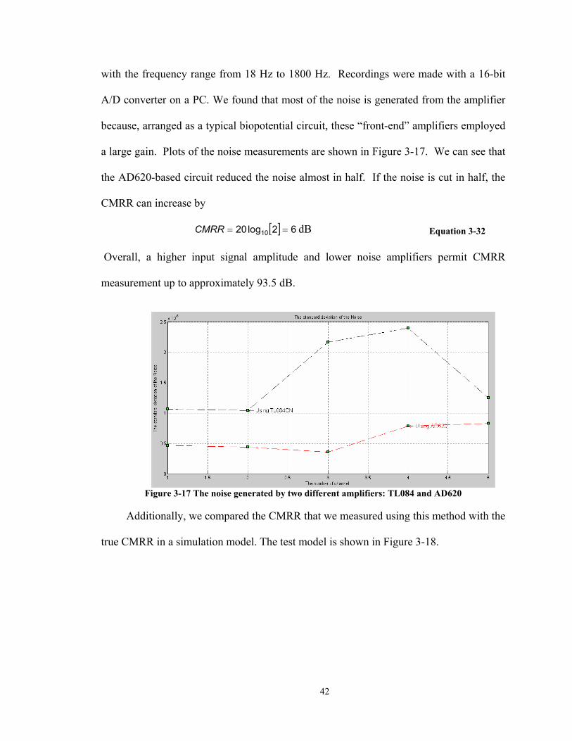
42

with the frequency range from 18 Hz to 1800 Hz. Recordings were made with a 16-bit

A/D converter on a PC. We found that most of the noise is generated from the amplifier

because, arranged as a typical biopotential circuit, these “front-end” amplifiers employed

a large gain. Plots of the noise measurements are shown in Figure 3-17. We can see that

the AD620-based circuit reduced the noise almost in half. If the noise is cut in half, the

CMRR can increase by

[ ] 62log20 10 ==CMRR dB Equation 3-32

Overall, a higher input signal amplitude and lower noise amplifiers permit CMRR

measurement up to approximately 93.5 dB.

Figure 3-17 The noise generated by two different amplifiers: TL084 and AD620

Additionally, we compared the CMRR that we measured using this method with the

true CMRR in a simulation model. The test model is shown in Figure 3-18.

43

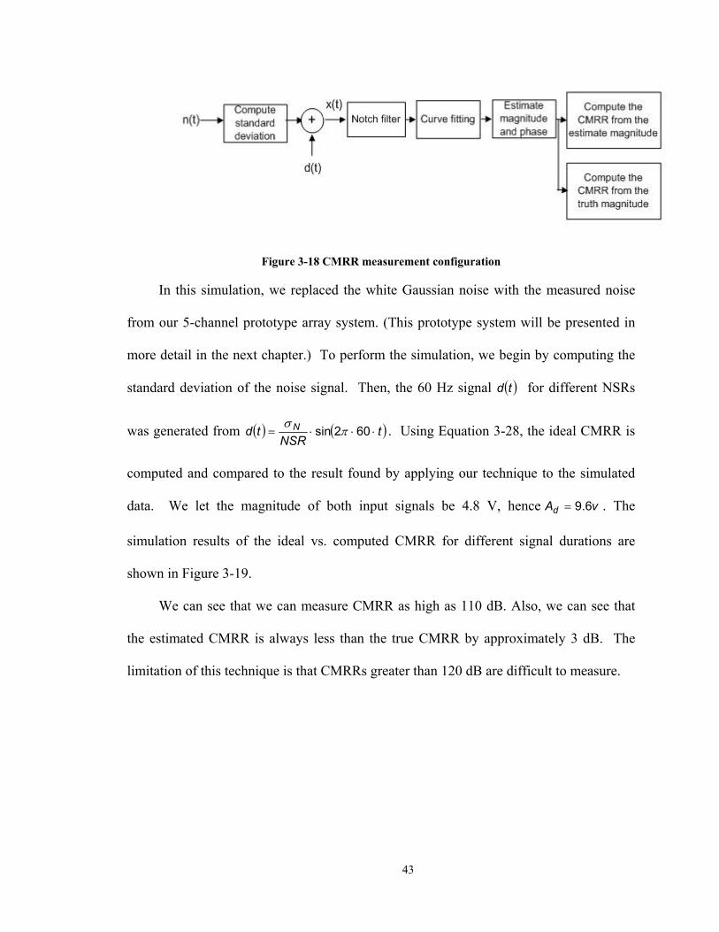
Figure 3-18 CMRR measurement configuration

In this simulation, we replaced the white Gaussian noise with the measured noise

from our 5-channel prototype array system. (This prototype system will be presented in

more detail in the next chapter.) To perform the simulation, we begin by computing the

standard deviation of the noise signal. Then, the 60 Hz signal ( )td for different NSRs

was generated from ( ) ( )tNSR

td N ⋅⋅⋅= 602sin πσ . Using Equation 3-28, the ideal CMRR is

computed and compared to the result found by applying our technique to the simulated

data. We let the magnitude of both input signals be 4.8 V, hence vAd 6.9= . The

simulation results of the ideal vs. computed CMRR for different signal durations are

shown in Figure 3-19.

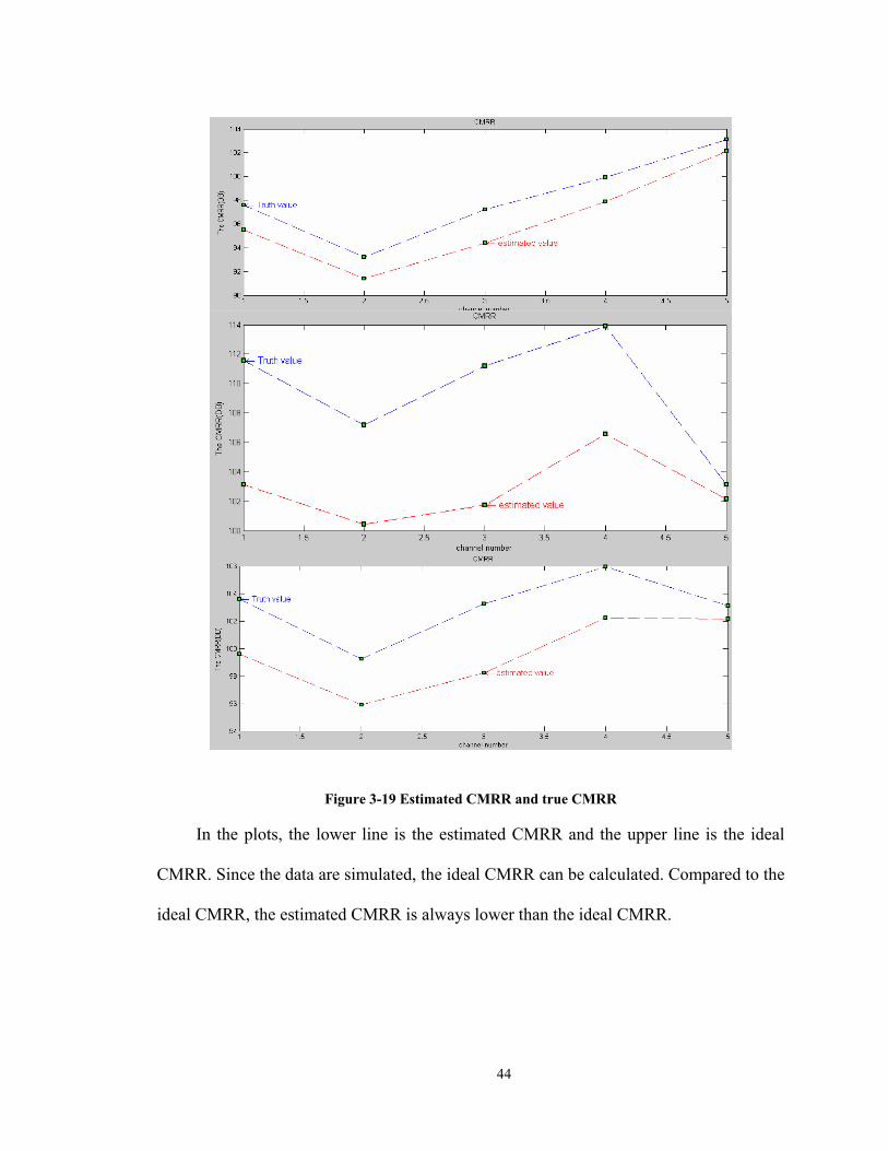
We can see that we can measure CMRR as high as 110 dB. Also, we can see that

the estimated CMRR is always less than the true CMRR by approximately 3 dB. The

limitation of this technique is that CMRRs greater than 120 dB are difficult to measure.

44

Figure 3-19 Estimated CMRR and true CMRR

In the plots, the lower line is the estimated CMRR and the upper line is the ideal

CMRR. Since the data are simulated, the ideal CMRR can be calculated. Compared to the

ideal CMRR, the estimated CMRR is always lower than the ideal CMRR.

45

3.2.4 Simulation Results Using Mixing Technique

In this section, the CMRR results are compared for different equalization filter

design techniques. The three major comparisons utilized:

• No software equalization,

• Equalization filter implemented with the conventional technique,

• Equalization filter implemented using the mixing technique.

Using linear shift technique to design the equalization filter in time domain

In this simulation, the noise level is 2 percent. The equalization filter is designed by

using the linear shift technique after the frequency response of the equalization filter is

determined. For each simulation, CMRR is calculated vs. the length of the FIR

equalization filter. The figure shows that using software equalization can improve the

CMRR significantly. With the mixing technique, the CMRR can be as high as 75 dB.

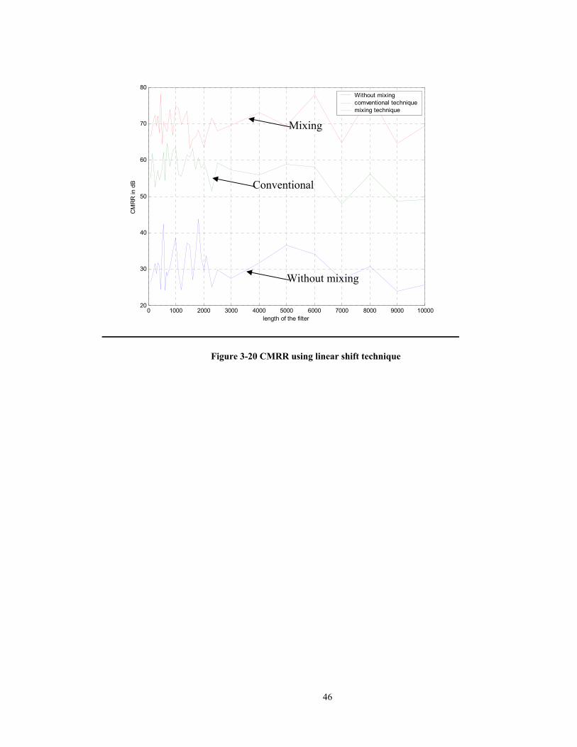
46

0 1000 2000 3000 4000 5000 6000 7000 8000 9000 1000020

30

40

50

60

70

80

length of the filter

CM

RR

in d

B

Without mixingcomventional techniquemixing technique

Figure 3-20 CMRR using linear shift technique

Mixing

Conventional

Without mixing

47

Using windowing technique to design the equalization filter in time domain

The next simulation is performed using the same conditions as above, except that

the equalization filter is designed using the simple windowing technique (i.e., absent the

linear shift). The figure also shows that using software equalization filter can improve the

CMRR and that the mixing technique achieves the highest CMRRs. When equalization

is performed, the linear shift operation produces superior equalization filters.

0 1000 2000 3000 4000 5000 6000 7000 8000 9000 1000020

25

30

35

40

45

50

55

60

65

70

lenght of the filter

CM

RR

in d

B

Without mixingcomventional techniquemixing technique

Figure 3-21 CMRR using windowing technique

Mixing

Conventional

Without mixing

48

CHAPTER 4 LABORATORY EXPERIMENTS

4.1 Hardware Introduction

All the laboratory data described above are recorded from a five-channel prototype

system. Each channel consists, in sequence, of four stages:

Stage 1: Eighth order, unit gain, Sallen-Key, Butterworth filter

with cut-off frequency at 15 Hz. This stage attenuates motion artifact

during severe movement conditions.

Stage 2: Selectable gain: There are eight selectable values. The

gain prior to the first high-pass filter stage is 10. Gain selection resolution

is a factor of two per step. Since the electrode-amplifier circuit is

designed for a gain of 100, the signal conditioning circuit’s gain can range

from 5–200. The different gain selections must be discrete in order to be

reproducible for use in channel equalization. The available set of gain

selections is: 2, 4, 8, 16, 32, 64, 128 and 256.

Stage 3: Electrical isolation: Provided by a unity-gain circuit

accepting inputs over the range of ±5 V.

Stage 4: Low-pass filter: Fourth-order, unity-gain, Sallen-Key,

Butterworth design with cut-off frequency at 1800 Hz.

The schematic of the circuits used in this project can be found in the appendix. In

this project, a Matlab program (capture_data.m [Mark]) is used to record the data via the

PC and A/D converter board.

In any hardware system, the most important issue is the inevitable presence of

broadband background noise in the calibration signal. Before any calibration data are

recorded, the noise level is measured for our prototype system by grounding the input of

49

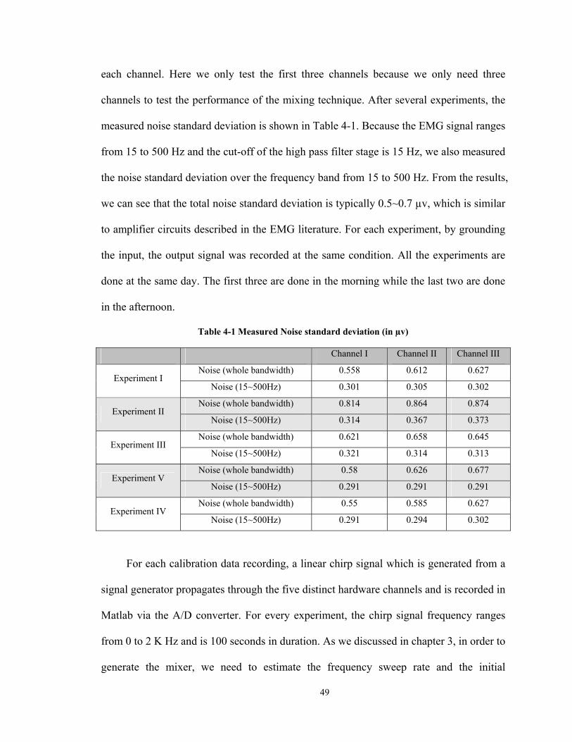
each channel. Here we only test the first three channels because we only need three

channels to test the performance of the mixing technique. After several experiments, the

measured noise standard deviation is shown in Table 4-1. Because the EMG signal ranges

from 15 to 500 Hz and the cut-off of the high pass filter stage is 15 Hz, we also measured

the noise standard deviation over the frequency band from 15 to 500 Hz. From the results,

we can see that the total noise standard deviation is typically 0.5~0.7 µv, which is similar

to amplifier circuits described in the EMG literature. For each experiment, by grounding

the input, the output signal was recorded at the same condition. All the experiments are

done at the same day. The first three are done in the morning while the last two are done

in the afternoon.

Table 4-1 Measured Noise standard deviation (in µv)

Channel I Channel II Channel III

Noise (whole bandwidth) 0.558 0.612 0.627 Experiment I

Noise (15~500Hz) 0.301 0.305 0.302

Noise (whole bandwidth) 0.814 0.864 0.874 Experiment II

Noise (15~500Hz) 0.314 0.367 0.373

Noise (whole bandwidth) 0.621 0.658 0.645 Experiment III

Noise (15~500Hz) 0.321 0.314 0.313

Noise (whole bandwidth) 0.58 0.626 0.677 Experiment V

Noise (15~500Hz) 0.291 0.291 0.291

Noise (whole bandwidth) 0.55 0.585 0.627 Experiment IV

Noise (15~500Hz) 0.291 0.294 0.302

For each calibration data recording, a linear chirp signal which is generated from a

signal generator propagates through the five distinct hardware channels and is recorded in

Matlab via the A/D converter. For every experiment, the chirp signal frequency ranges

from 0 to 2 K Hz and is 100 seconds in duration. As we discussed in chapter 3, in order to

generate the mixer, we need to estimate the frequency sweep rate and the initial

50

frequency for the original chirp signal, so the signal from the generator is also recorded to

provide the necessary information. Hence for each recording, there are six channels of

data presented. The first five channels are from the respective hardware channels and the

sixth channel is a direct sampling of the signal generator output. Because the start time of

the chirp signal can not be perfectly synchronized, we allotted additional recording time

beyond the desired recording duration. This additional recording “buffer” is removed

prior to any signal processing.

The voltage range of our A/D converter is ±5V. Our prototype system has a

minimum gain of 10 and a maximum gain of 2560. Thus, the maximum voltage of the

input is mvv 95.12560/5 = , while the minimum voltage that the signal generator can

produce is 50 mV. Therefore, the interface between the signal generator and the input of

the system is not directly connected. To satisfy the voltage requirement, the output of the

signal generator was passed through a two-resistor voltage divider circuit, and from there

into the prototype system.

The data are saved into a .daq file in the Matlab format. The sampling rate is always

4096 samples/second. The recording apparatus are arranged as shown in Figure 4-1.

Figure 4-1 Recording processing model

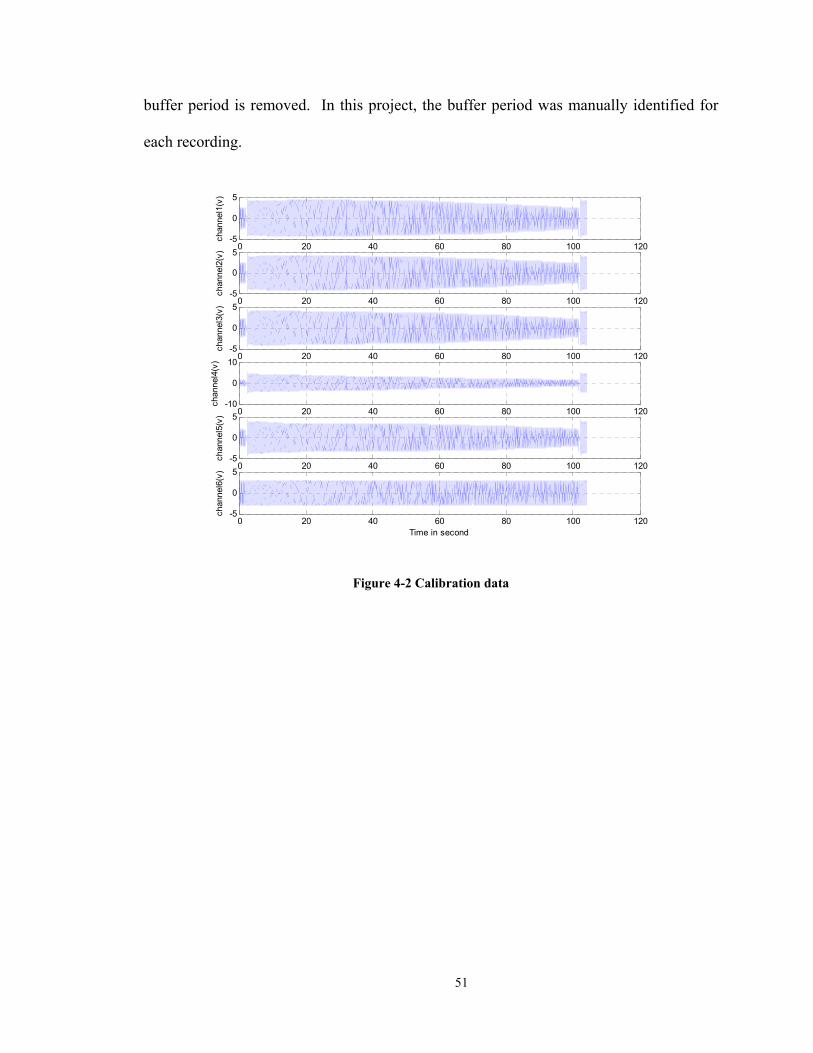
Figure 4-2 shows an example of the six acquired channels using a 100 second recording

duration plus a 5 second buffer time. Figure 4-3 shows the calibration data after the

Signal generator

Resistor divider

Prototype system

A/D

Matlab

51

buffer period is removed. In this project, the buffer period was manually identified for

each recording.

0 20 40 60 80 100 120-5

0

5

chan

nel1

(v)

0 20 40 60 80 100 120-5

0

5

chan

nel2

(v)

0 20 40 60 80 100 120-5

0

5

chan

nel3

(v)

0 20 40 60 80 100 120-10

0

10

chan

nel4

(v)

0 20 40 60 80 100 120-5

0

5

chan

nel5

(v)

0 20 40 60 80 100 120-5

0

5

chan

nel6

(v)

Time in second

Figure 4-2 Calibration data

52

0 10 20 30 40 50 60 70 80 90 100-5

0

5

chan

nel1

(v)

0 10 20 30 40 50 60 70 80 90 100-5

0

5

chan

nel2

(v)

0 10 20 30 40 50 60 70 80 90 100-5

0

5

chan

nel3

(v)

0 10 20 30 40 50 60 70 80 90 100-5

0

5

chan

nel4

(v)

0 10 20 30 40 50 60 70 80 90 100-5

0

5

chan

nel5

(v)

0 10 20 30 40 50 60 70 80 90 100-5

0

5

chan

nel6

(v)

Time in second

Figure 4-3 Calibration data after carving out the buffer

The equalization filter design configuration is shown as Figure 4-4.

Figure 4-4 Configuration for equalization filter design

Note that the sixth channel that directly comes from the signal generator was used to

estimate the sweep rate, initial frequency and the phase. They were estimated using a

Calibration data

Carve out the buffer

Channel #1

Channel #5

Channel #6

Estimate the sweep rate and initial frequency

Construct MIXER

Mixing with the mixer

LPF

Mixing with the mixer

LPF

53

nonlinear least squares fit to a prototype chirp (Matlab optimization toolbox). A precise

initial guess should be given when using this method.

54

4.2 Experiment Results

In this section, we compare the results between using the conventional technique

and the mixing technique. The data used in this analysis were recorded on July 11, 2004

(file name: “ch0711.daq”).

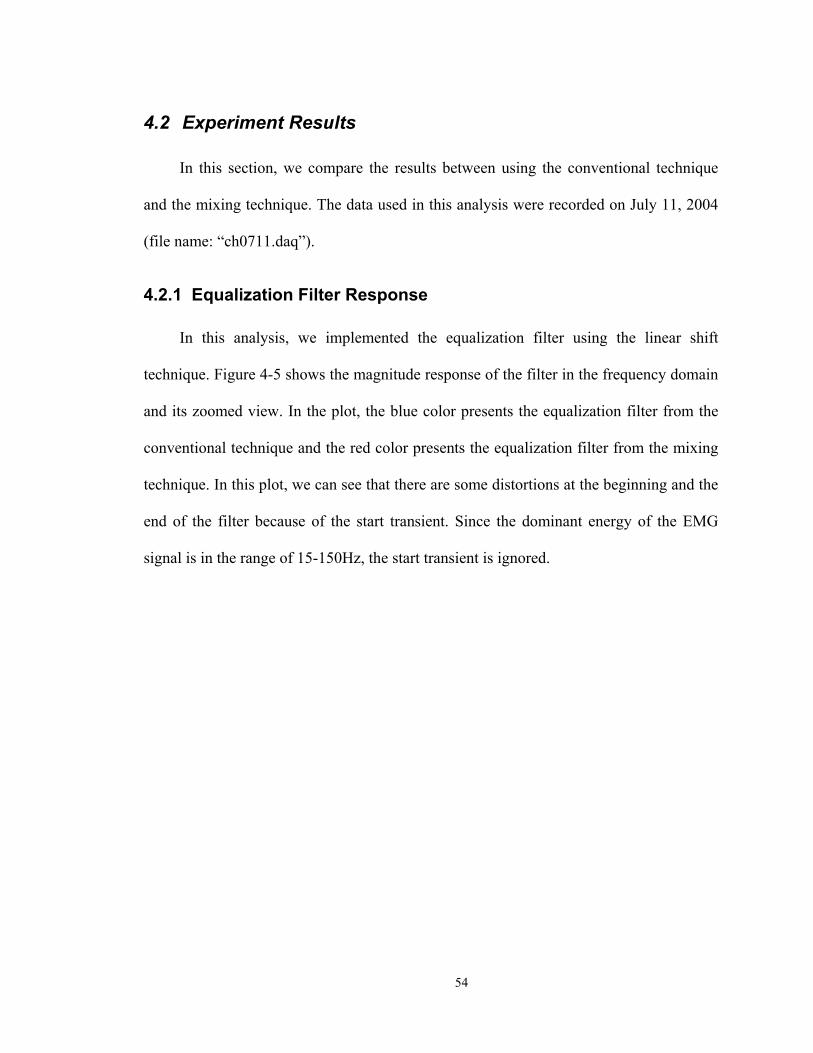
4.2.1 Equalization Filter Response

In this analysis, we implemented the equalization filter using the linear shift

technique. Figure 4-5 shows the magnitude response of the filter in the frequency domain

and its zoomed view. In the plot, the blue color presents the equalization filter from the

conventional technique and the red color presents the equalization filter from the mixing

technique. In this plot, we can see that there are some distortions at the beginning and the

end of the filter because of the start transient. Since the dominant energy of the EMG

signal is in the range of 15-150Hz, the start transient is ignored.

55

Figure 4-5 Magnitude response of the equalization filter

4.2.2 CMRR Results

In this section, we only show the results using the linear shift technique. The calibration

data named “ch0711.daq” is used to design the equalization filter using linear shift

technique. Two 60 Hz sine wave signal named “sin0711.daq” and “sin0712.daq” are used

to evaluate the equalization filter. Each recording has 100 seconds duration. Sine it is five

channel prototype, each 60 Hz sine wave can be perform several bipolar configuration.

The CMMR is the mean value of all the bipolar configuration.

Conventional technique Mixing technique

CMRR 35dB 72dB

Without mixing

Zoomed view With mixing

56

CHAPTER 5 PRELIMINARY RESULTS From A 28-

CHANNEL ELECTRODE ARRAY

5.1 EMG hardware system

5.1.1 The EMG Array

In this project, a 28-channel electrode array is also used to recode the EMG signal.

In this section, the preliminary results using the mixing technique with this array will be

described. The array was constructed as a 4x7 rectangular grid. Each electrode consisted

of a stainless steel M2 screw arranged 5 mm center to center from adjacent electrodes.

Each electrode was connected to a gain of 20, high-impedance differential amplifier

(Analog Devices AD620 Instrumentation Amplifier). To achieve a monopolar

configuration, the second input to each differential amplifier was from a common

monopolar reference electrode. An additional electrode served as the isolated power

supply reference. These additional electrode contacts were also stainless steel. The

electrodes and amplifiers were mounted on a printed circuit board (PCB) which was

epoxy encapsulated. Flexible wiring cables connected this pre-amplifier to the signal

conditioning apparatus.

A one layer PCB board is designed. There are 14 channels on each side. Figure 5-1

shows the schematic of the top of the array PCB board and Figure 5-1 shows the

completed electrode array used in this project.

57

Figure 5-1 The schematic of one side of the array PCB board

Figure 5-2 The electrode array

58

5.1.2 Signal Conditional Circuits

The design of the signal conditioning circuits is identical to the circuits presented in

chapter 4. In this research, four conditioning circuits were built into one signal

conditioning unit via a PCB implementation of the circuit design. All units were

powered from two power supplies, one of which maintained electrical isolation from

earth ground.

5.2 Experiment Results

Prior to each experiment, conductive electrical gel is applied to the electrode and

the skin to reduce the electrode-skin impedance. Each EMG recording is 5 seconds long

and the calibration data are 100 seconds long (plus the buffer duration). Figure 5-3

shows a sample EMG recording from our 28-channel array. The x-axis is the time vector

in seconds and y-axis is the magnitude of the EMG signal. Figure 5-4 and Figure 5-5

show that equalized EMG signal of one channel wit bipolar and NDD configuration.

Figure 5-6 and Figure 5-7 show one of the channels with NDD spatial filter before and

after equalization. The plots show that with equalization, the MU can be easily identified.

59

Figure 5-3 28 channels EMG signal review

Figure 5-4 Equalized EMG signal (Bipolar) Right side is the zoomed view

Figure 5-5 Equalized EMG signal (NDD) Lower is the zoomed view

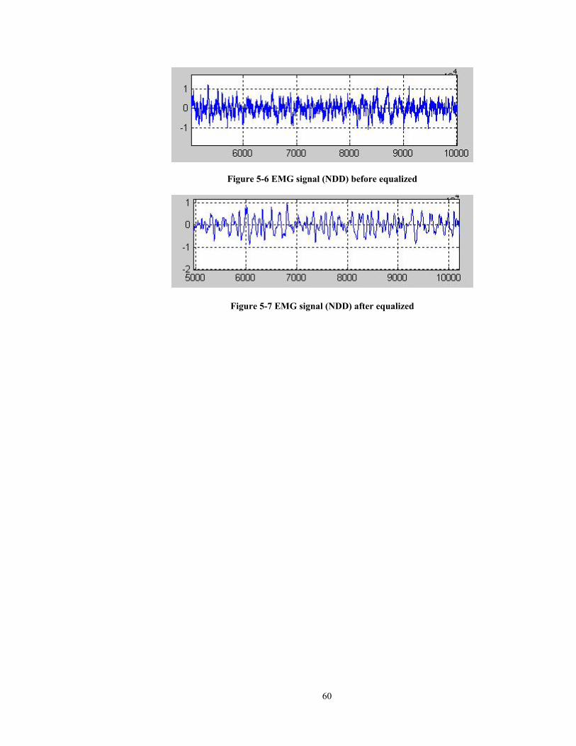
60

Figure 5-6 EMG signal (NDD) before equalized

Figure 5-7 EMG signal (NDD) after equalized

61

CHAPTER 6 CONCLUSIONS AND FUTURE WORK

6.1 Discussion

In this section, we briefly summarize the conclusions drawn from this project. In

recent years, there has been increasing interesting in detecting single MU activity via

noninvasive spatial filtering techniques. In general, the spatial filtering is implemented in

hardware. Due to the limitations in hardware, we sought to achieve high-quality, flexible

spatial filtering using software channel equalization. We explored different techniques to

design the equalization filter. Our conventional technique consisted of taking the ideal

frequency response divided by the measured frequency response to determine the

frequency response of the equalization filter. We showed that conventional channel

equalization can improve the CMRR, but not sufficiently so and it is very sensitive to

noise.

Since the major problem is broadband background noise, it became necessary to

eliminate as much noise as possible before implementing the equalization filter. Thus, we

pursued de-noising via a mixing technique. This new technique is evaluated with both

simulation and laboratory experiments. From the results shown in chapter 3 and chapter 4,

it is clearly observed that the mixing technique can improve CMRR more than the

conventional technique and it is much less sensitive to noise. In this project, we are

typically achieving a CMRR of 64-85 dB at 60 Hz after mixing and equalization, but less

than 40 dB with conventional equalization.

62

6.2 Future Work

First, based on the previous discussion, the premise of our software mixing

technique has been demonstrated. The mixer requires the initial frequency of the

excitation chirp and its sweep rate. We found our results to be sensitive to the accuracy of

determining these parameters via an optimization algorithm. In the future, we can either

use a new algorithm to estimate them, or produce a better initial guess when using the

Matlab optimization toolbox.

Second, to eliminate the noise, we can consider using a linear time-varying band-

pass filter (LTV). By using this technique, there exits a trade-off between the amount of

noise reduction and the amount of signal distortion. Preliminary simulations for testing

the noise reduction performance of LTV filters suggested that a smaller passband reduced

most of the noise, but caused large signal distortion. High-order LTV filters can

significantly improve these issues, but might result in an unacceptable start up transient.

But, we could alternatively use a low-order LTV filter cascaded with our mixing

technique. In the future, we can measure the performance via the use of LTV filters

together with our mixing technique.

Third, the most difficult challenge in the mixing technique is the low pass filter

design stage, since the cut-off frequency of the low pass filter must be set to less than 1%

of the Nyquist frequency. Currently the order of the low pass filter is greater than 3000.

In the future, we may investigate a better technique to design the low pass filter.

Fourth, we find that the achieved CMRR is much better if the calibration data

duration is longer. Currently, we are using a 100 second chirp signal to calibrate the

equalization filter. By using longer duration data recordings with a slower frequency

63

ramp, we can use larger order low-pass filters after the mixer to eliminate more noise

(because a longer filter startup transient can be tolerated). Another possible solution is to

use two 50 second duration chirps instead of one 100 second duration chirp. The first

chirp could ramp in frequency from 0 to 500 Hz and the other one from 500 to 2 KHz.

Their resulting transfer function could be assembled in the frequency domain to provide

information over the complete frequency range. Finally, we might consider upsampling

the signal prior to the mixing stage to determine if low-pass filters implemented at the

upsampled rate can reduce the effective startup transient duration.

64

REFERENCES

[Clancy01] Edward A. Clancy, Hongfang Xia and Mark V. Bertolina, "A

Preliminary Report on the Use of Equalization Filters to Derive High Spatial

Resolution Electrode Array Montages," Proceedings of the International

Symposium on Neuromuscular Assessment in the Elderly Worker (NEW), Torino,

Italy, pp. 103−106, February 20–21, 2004.

[DeLuca79] Carlo J. De Luca, Physiology and Mathematics of Myoelectric

Signals. IEEE Trancations on Biomedical Engineering, Vol. BME-26, NO. 6,

June 1979.

[DeLuca02] Carlo J. De Luca. Surface Electromyography: Detection and

Recording. 2002 by DelSys Incorporated.

[Disselhorst97] Catherine Disselhorst-Klug, Jiri Silny, and Gunter Rau,

Improvement of Spatial Resolution in Surface-EMG: A Theoretical and

Experimental Comparison of Different Spatial Filters. IEEE Trans. Biomed.

Eng., Vol. 44, No. 7, July 1997.

[Disselhort98] Catherine Disselhort-Klug, Gunter Rau, Astrid Schmeer, Jiri

Silney. Non-invasive detection of the single motor unit action potential by

averaging the spatial potential distribution triggered on a spatially filtered motor

unit action potential. Journal of Electromyography and kinesiology 9(1999) 67-

72.

[Hambley] Allen Hambley. Electronic 2nd Edition. Prentice Hall 1999.

[Mark] Mark V. Bertolina, Khoi Le, Hai Trinh. Active Power-Line Interface

Attenuation in Bioamplifiers. Project Number: EXC-0201-EE.

65

[Met90] A. C. MettingVanRijn, A. Peper, C. A. Grimbergen. High Quality

Recording of Bioelectric Events. I: Interference Reduction, Theory and Practice.

IEEE Medical & Biological Engineering & Computing, vol. 28 pp. 389-394,

http://www.biosemi.com/publications/artikel3.htm, Sept. 1990.

[Neuman] Neuman, MR. Biopotential Electrodes. The biomedical Engineering

Handbook, Second Edition 48: 1-12.

[Proakis96] John G. Proakis, Dimitris G. Manolakis, Digital Signal Processing

Principles, Algorithms, and Applications 3rd Edition. Prentice Hall ISBN 0-13-

373762-4.

[Rabiner] Lawrence R. Rabiner, Bernard Gold and C. A. McGonegal. An

Approach to the Approximation Problem for Nonrecursive Digital Filters. IEEE

Transactions on Audio and Electroacoustics. Vol. AU-18, No. 2 June 1970.

[Rau97] G. Rau and C. Disselhorst-klug. Principles of High-Spatial-Resolution

Surface EMG (HSR-EMG): Single Motor Unit Detection and Application in the

Diagnosis of Neuromuscular Disorders. J. Electromyogr. Kinesiol. Vol. 7, No. 4,

pp. 233-239, 1997.

[Reucher86] Rau G, Reucher H, Schneider J, Silny J. Design and application of

spatially filtering EMG electrode configurations. In: Proceedings of Eighth

Annual Conference of the Engineering in Medicine and Biology Society. Fort

Worth, 1986:522-5.

[Reucher87] H. Reucher, G Rau, and J. Silny. Spatial Filtering of Noninvasive

Nultielectrode EMG: part I-Introduction to Measuring Technique and

Applications. IEEE Trans. Biomed. Eng., vol. BME-34, No. 2, pp98-105, 1987.

66

[Reucher87b] H. Reucher, J. Silny and G. Rau. Spatial Filtering of Noinvasive

Multielectrode EMG: Part II-Filter Performance in Theory and Modeling. IEEE

Trans. Biomed. Eng., vol. BME-34, No. 2, pp106-113, 1987.

[Scott] Dr. Scott Day. Important Factors in Surface EMG Measurement. Bortec

Biomedical Ltd. 225, 604-1st ST SW Calgary, AB T2P 1M7. www.bortec.ca.

[Stalberg80] Stalberg E, Antoni L. Electrophysiological cross section of the

motor unit. J Neurol Neurosurg Psychiatry 1980; 43:469-74.

[Texas] Texas Instruments, Analysis of the Sallen-Key Architecture Application

Report. July 1999 – revised September 2002.

[Webster73] James C. Huhta and John G. Webster. 60-Hz Interference in

Electrocardiography. IEEE Transactions on Biomedical Engineering, Vol. BME-

20, No. 2, March 1973.

[Webster83] Winter, Bruce B., Webster, John G. Driven-Right-Leg Circuit

Design. IEEE Trans, Biomed. Eng., Vol. BME-30 pp. 62-66, January 1983.

[Webster99] Webster, John G. The measurement, Instrumentation, and Sensors

Handbook. Sec. 74. 1999.

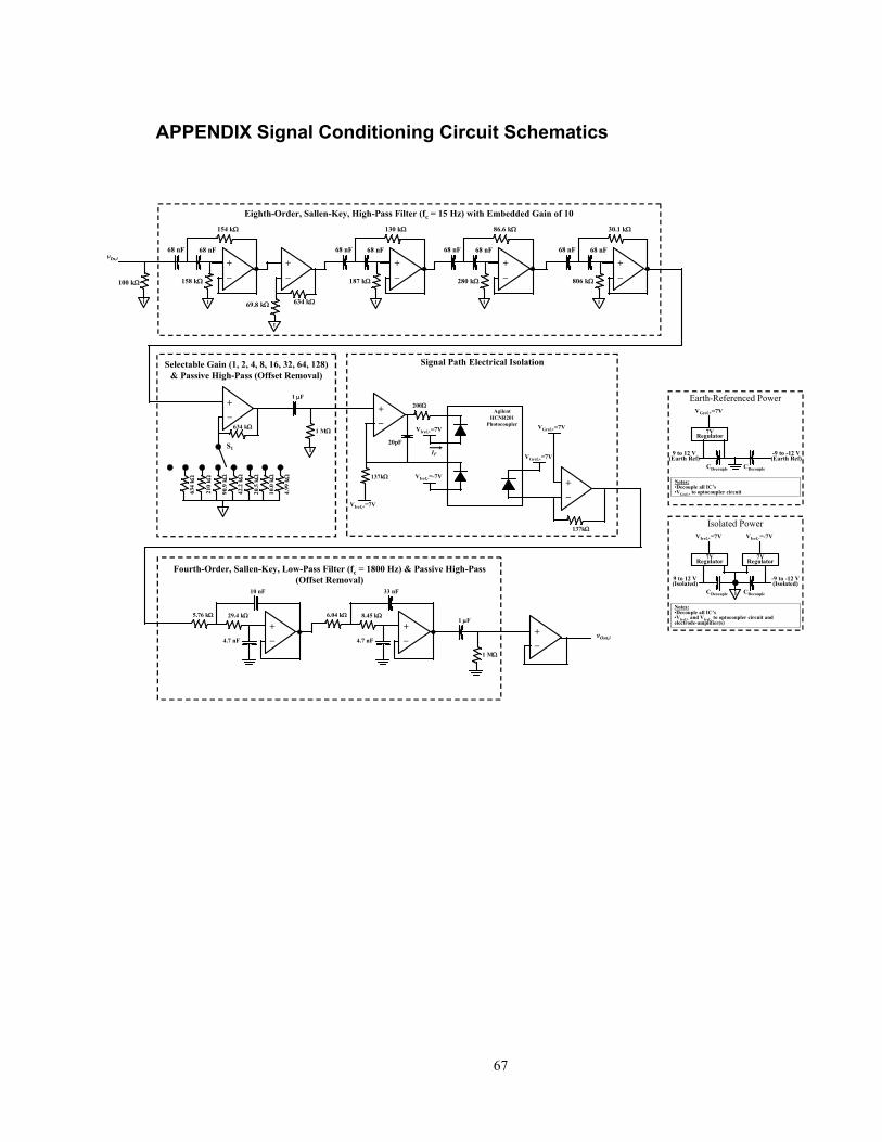
67

APPENDIX Signal Conditioning Circuit Schematics

+_

68 nF 68 nF

30.1 kΩ

806 kΩ

I

+_

68 nF 68 nF

86.6 kΩ

280 kΩ

I

+_

68 nF 68 nF

130 kΩ

187 kΩ

I

+_

vIn,i

68 nF 68 nF

154 kΩ

158 kΩ

I

+_

634 kΩ69.8 kΩ

I

Eighth-Order, Sallen-Key, High-Pass Filter (fc = 15 Hz) with Embedded Gain of 10

+_

634 kΩ

I

634

kΩ

S1

210

kΩ

90.9

kΩ

42.2

kΩ

20.5

kΩ

10.0

kΩ

4.99

kΩ

1 µF

1 MΩ

I

Selectable Gain (1, 2, 4, 8, 16, 32, 64, 128) & Passive High-Pass (Offset Removal)

IF

AgilentHCNR201

Photocoupler

+_

+_

VIref,+=7V

VIref,+=7V

VIref,-=-7V

VGref,+=7V

VGref,+=7V

137kΩ

200Ω

137kΩ

20pF

Signal Path Electrical Isolation

+_4.7 nF

10 nF

29.4 kΩ5.76 kΩ

+_4.7 nF

33 nF

8.45 kΩ6.04 kΩ1 µF

1 MΩ

vOut,i

Fourth-Order, Sallen-Key, Low-Pass Filter (fc = 1800 Hz) & Passive High-Pass (Offset Removal)

100 kΩ

I

+_

ICDecouple CDecouple

9 to 12 V(Isolated)

-9 to -12 V(Isolated)

7VRegulator

7VRegulator.

VIref,+=7V VIref,-=-7V

Notes:•Decouple all IC’s•VIref,+ and VIref,- to optocoupler circuit and electrode-amplifier(s)

Isolated Power

Notes:•Decouple all IC’s•VGref,+ to optocoupler circuit

Earth-Referenced Power

CDecouple CDecouple

9 to 12 V(Earth Ref)

-9 to -12 V(Earth Ref)

7VRegulator

VGref,+=7V