the use of model, gis and remote sensed data in the society · landscape approach mirrors these...
TRANSCRIPT
The use of model, GIS and remote sensed data in the society –
examples from land use planning and flood management
Dagmar Haase Department of Computational Landscape Ecology
METIER Training Lecture, Helsinki, November 6, 2008
Page 2
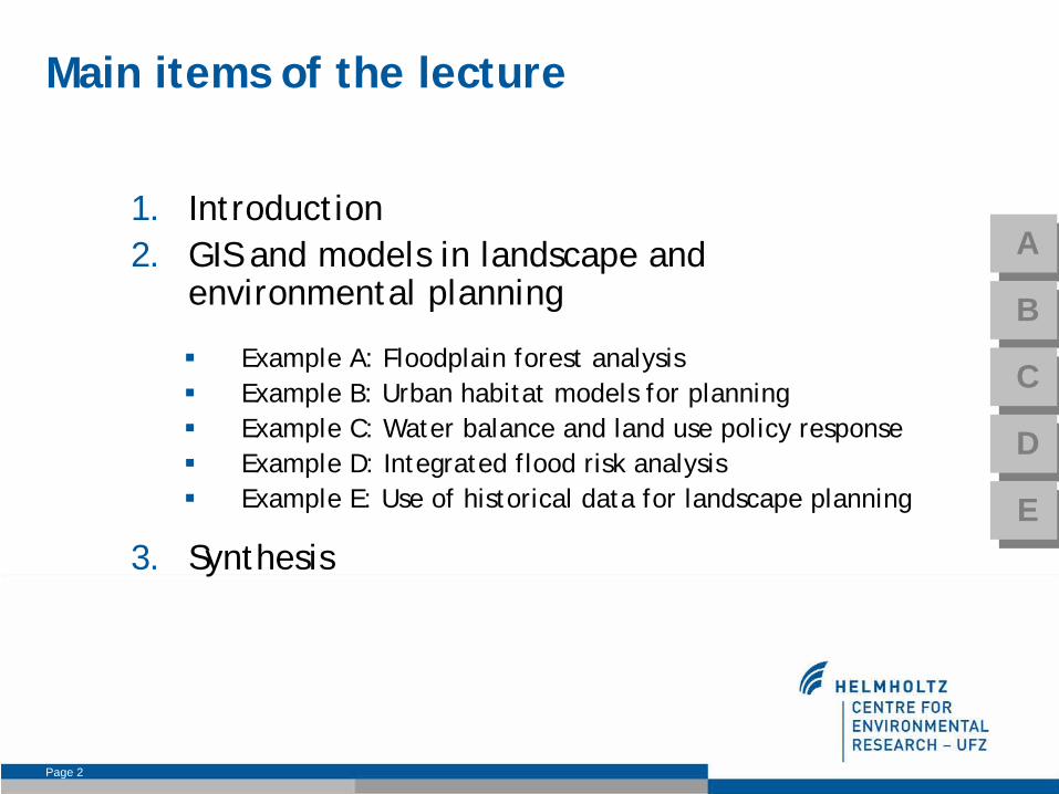
Main items of the lecture
1.
Introduction2.
GIS and models in landscape and environmental planning
Example A: Floodplain forest analysis Example B: Urban habitat models for planningExample C: Water balance and land use policy responseExample D: Integrated flood risk analysisExample E: Use of historical data for landscape planning
3.
Synthesis
A
B
C
D
E

Page 3
Introduction …
about my work
Major challenges for landscape management, resource protectionand land use related research are processes and pattern of
Global change (climate change, emissions, resource exploitationdemographic change and urbanisation a.o.)
Hot spots of change: (Mega)Cities, rural landscapes in Europe
Landscape approach mirrors these challenges since it is an integrative approach
My work bases on the ideas of a.o. Naveh (2001), Brandt (2001), Wu & Hobbs (2002), Ravetz (2000), Müller et al., (2007).
Modern landscape research involves both natural and social sciencecomponents, qualitative and quantitative methodologies.

Page 4
Major research questions
What are the main drivers of land use and lansdscape change today, in the next future, and
how can we learn from historic changes?
How do form, pattern and heterogeneity of land uses affect environmental performance, ecosystem services and resource availability?
What models and tools can we apply to contribute to land use planning, river basin and flood(plain) management?
Page 5
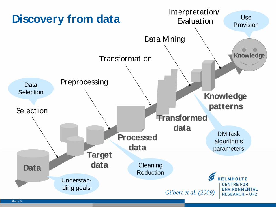
Discovery from data
Gilbert et al. (2009)
DataData
Selection
TargetTarget datadata
Preprocessing
ProcessedProcessed datadata
Transformation
TransformedTransformed datadata
Data
Mining
KnowledgeKnowledge patternspatterns
Interpretation/ Evaluation
KnowledgeKnowledge
Understan- ding goals
Data Selection
Cleaning Reduction
DM task algorithms parameters
Use Provision

Page 6
Geospatial analytical tools
Joima et al. (2009)
Computational cartography
Statistical
computingSpatial
StatisticsVisualisation
Mapping Querying Transformations Descriptive
summaries
Raster algebra Cartographic
modellingNetwork
analysisSpatial
interpolation
Terrain analysis
Hydrological
analysisSpatial
data
miningSpatial
modelling
Geospatial
image processing
Web GISArcGIS SAGA GIS
SELES 3.2beta R Repast

Page 7
Working on cycles and causalities Example: Land consumption and land cycling policy
TRANSFORMATION OF LAND USES
IMPACT ecosystems, water fluxes, soil, economy, quality of
life, political pressure
PRESSURE STATE
ASSESS- MENT of impacts
natural RESPONSE
GOVERNANCE Intervention by policy making
and planning
modified RESPONSE
DRIVERS economy, demography, living
habits, land use policies, planning instruments

Page 8
GIS and models in landscape research: how we apply it
GIS data in planning
Spatially explicit or non-explicit model
Output data = spatial shape of the simulation result
Spatial sh
ape
of dynam
ics
and change
Modelling:
neighbourhood relations
of cells; HRU’s etc
Spatial shape
of a problem
or a component
( )
( )∑
∑
=
=
∗
∗∗= n
iii
n
iiii
GWKAK
verGWKAKF
1
1
filtering capacity

Page 9
References
McIntosh, B.S., Giupponi, C., Voinov, A.A., Smith, C., Matthews, K.B., Monticino, M., Kolkman, M.J., Crossman, N., van Ittersum, M., Haase, D., Haase, A., Mysiak, J., Groot, J.C.J., Sieber, S., Verweij, P., Quinn, N., Waeger, P., Gaber, N., Hepting, D., Scholten, H., Sulis, A., van Delden, H., Gaddis, E., Assaf, H. 2009. Bridging the gap: developing tools for environmental policy and management, In: Jakeman, T., Rizzoli, A., Voinov, A. & Chen (eds.) 2009. State of the Art and Futures in Environmental Modelling and Software, Elsevier.
Nuissl, H., Haase, D., Wittmer, H., Lanzendorf, M. 2008. Impact assessment of land use transition in urban areas –
an integrated approach
from an environmental perspective. Land Use Policy, doi:10.1016/j.landusepol.2008.05.006.

Page 10
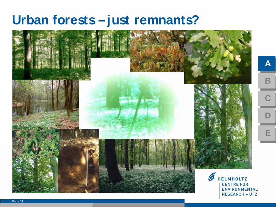
Example A: Remnants of floodplain forests?
A GIS model approach.
A
B
C
D
E
Page 11
Urban forests –
just remnants?
A
B
C
D
E
Page 12
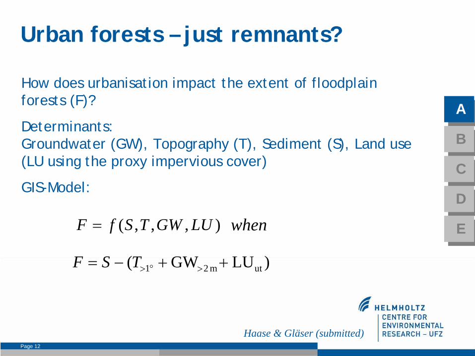
Urban forests –
just remnants?
How does urbanisation impact the extent of floodplain forests (F)?
Determinants: Groundwater (GW), Topography (T), Sediment (S), Land use (LU using the proxy impervious cover)
GIS-Model:
),,,( LUGWTSfF =
)LUGW( utm21 ++−= >°>TSF
when
Haase & Gläser (submitted)
A
B
C
D
E

Page 13
Urban forests –
just remnants?Classification criteria
Haase & Gläser (submitted)
A
B
C
D
E
Criterium Flood
sediment
Topography Ground-
water
level
Land use Natural-
ness
Inclusion
criterion
(threshold)
Occurrence no relief energy, difference to the surrounding terraces
<2.0 meters
(Vega/
Gley soils)
floodplain forest, wetlands, urban green spaces, parks, sports and leisure grounds, cemeteries
typical and relatively typical; low degree of imper-
viousness
Exclusion
criterion
(threshold)
No occurrence
relief
energy>5%
>2.0 meters
allotments, farmland, waste-
land, ruderal and succession areas, built-up areas (housing, transport, trade and industry)
relatively untypical and non typical; high degree of imper-
viousness
Range 0 …
1 0 …
5% 0 …
2.0 m
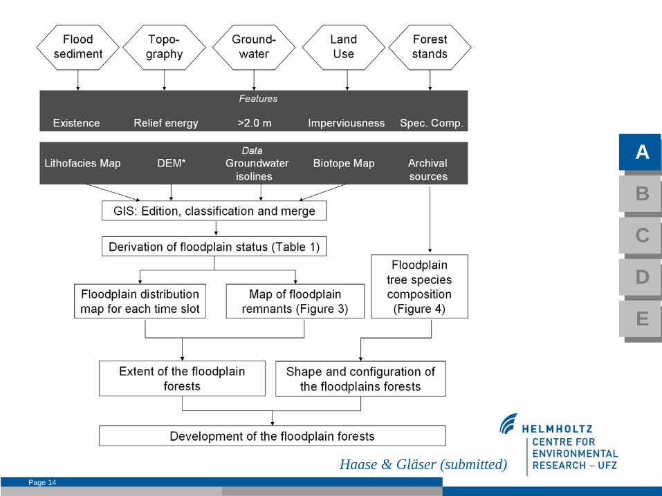
Page 14
Haase & Gläser (submitted)
A
B
C
D
E

Page 15
Urban forests –
just remnants?
Haase & Gläser (submitted)
A
B
C
D
E

Page 16
A
B
C
D
E
References
Haase, D. 2003. Holocene floodplains and their distribution in urban areas –
functionality indicators for their retention potentials.
Landscape & Urban Planning 66, 5-18.
Haase, D., Gläser, J. Determinants of floodplain forest development illustrated by the example of the floodplain forest in the District of Leipzig. Forest Ecology and Management.
Page 17
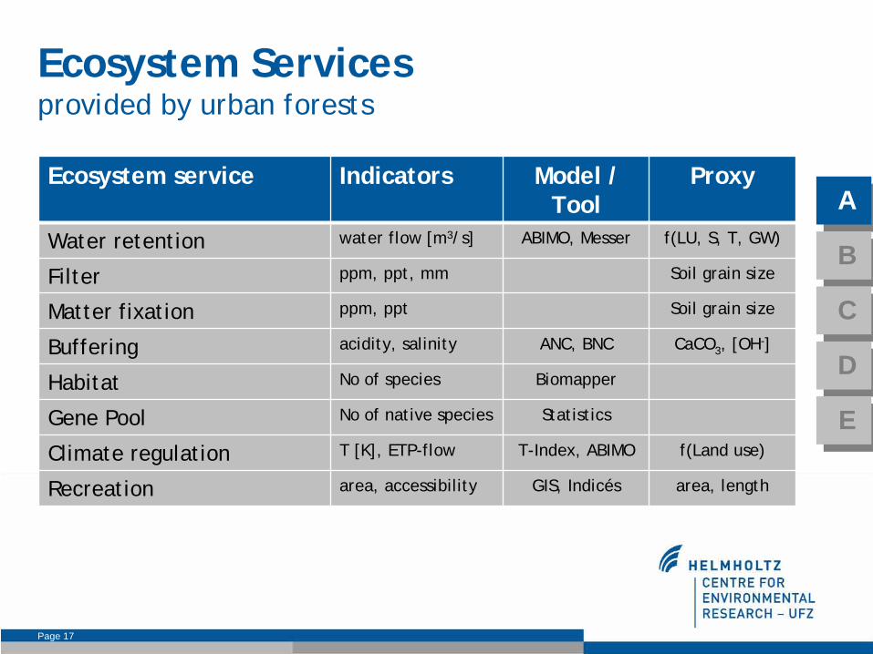
Ecosystem Services provided by urban forests
Ecosystem service Indicators Model / Tool
Proxy
Water retention water
flow
[m3/s] ABIMO, Messer f(LU, S, T, GW)
Filter ppm, ppt, mm Soil
grain
size
Matter fixation ppm, ppt Soil
grain
size
Buffering acidity, salinity ANC, BNC CaCO3
, [OH-]
Habitat No of species Biomapper
Gene Pool No of native species Statistics
Climate
regulation T [K], ETP-flow T-Index, ABIMO f(Land
use)
Recreation area, accessibility GIS, Indicés area, length
A
B
C
D
E

Page 18
Climate regulation
CO2
Global scalesequestration/storage of greenhouse gases
solar radiation
latent heat
Local scalereflectance evapotranspiration
A
B
C
D
E

Page 19
Climate regulation
Indicator: Climate Regulation represented by temperature value
Each land use type is assigned an average surface temperature taken from literature. The values are validated with thermal images for Leipzig.
Land use Temperature index
Continuous
urban fabric 1.2
Discontinuous
urban fabric 1.1
Industrial or
commerical
units 1.2
Forest 1.0
Parks 0.9
Water 0.8
(Kottmeier et al., 2007)
A
B
C
D
E

Page 20
Climate regulation
0 5 10 15 202,5
Kilometers
¯
Temperature index0.8
1.0
1.1
1.2
Since we assume that forest land use can reduce air temperatures best by emitting “sensitive” water flows in form of water vapor the index shows how much higher the land surface temperatures of any land use x are compared to forest
Model:
Index = T (land use x) / T (forest)
A
B
C
D
E

Page 21
Conclusions for Example A
Geospatial data and GIS are suitable data bases and tools to answer questions of landscape planners, water managersand urban foresters.
For implementation of the concept of Ecosystem Services the mapping of urban forests (re)gains importance.
GIS serves a a very suitable tool for visualising geospatialand landscape (ecological) and resource related contexts.
Land use data provide a helpful basis for model transfer on e.g. Ecosystem Services.
A
B
C
D
E

Page 22
Example B: Urban habitat modeling and
planning of green infrastructure
A
B
C
D
E

Page 23
Faunistic issues are rarely considered in urban landscape planning.
We find today an increasing isolation of urban habitats (… and >75% of urban inhabitants in the EU).
Aim: To incorporate species related nature protection and habitat suitability evaluation in urban planning innovative methodologies are necessary that work with minimum data requirements.
Hypothesis: Distribution and occurrence of species requires a defined parameter setting – although many organisms have a tolerance to their environment, the space is limited.
How habitat modeling supports planning?
A
B
C
D
E

Page 24
ENFA (Ecological Niche Factor Analysis)
Ecological Niche = ∑
cells with a certain probability of presenceData ...
for the species (Presence/Absence data)Boolean values0 = species does not occur (absent)1 = species occurs (present)
for the environment (EGV)continuous values of every variable
fundamental niche: Hyper volume in a n-dimensional space given though environmental parameter settings (Hutchinson, 1957)
environmental parameter settings are specific for every species
physiologic optimum (Walter, 1970)
A
B
C
D
E
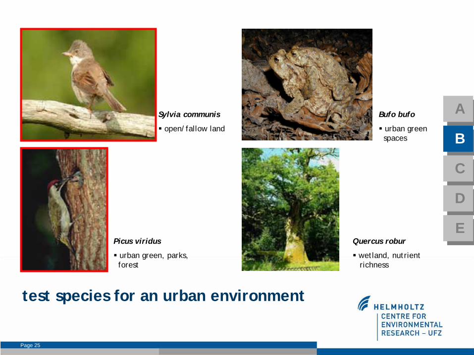
Page 25
Sylvia communis
open/fallow land
Picus viridus
urban green, parks, forest
Bufo bufo
urban greenspaces
test species for an urban environment
Quercus robur
wetland, nutrient richness
A
B
C
D
E

Page 26
urban structure fauna: species
parks, fallow land birds (Picus viridus)
GIS: ArcView, ArcInfo, Erdas Imagine, FRAGSTATS, Biomapper
ENFA (Ecological Niche Factor Analysis)
Methodology to create HS-maps
HS-maps: classification of the HSI summing up all cells with median values than: HSI: 0 ≤
HSI ≤
1
probability of the species occurrencefor DS in urban landscape planning
A
B
C
D
E

Page 27
Methodological approach
Vorher: (Auflösung 2 x 2 m) Nachher: (Auflösung 30 x 30 m)
Rasterkonvertierung (SUMMARY)
Berechnung neuer Rasterwerte (Mittelwertsberechnung – „Mean“)30 m
30 m
30 m
30 m
Raster - „fishnet“ (30 x 30 m)2x2m 30x30m
SUMMARY MEAN
GIS and data integration

Page 28
Methodological approach
Spatial input data
A
B
C
D
E

Page 29
Methodological approach
Landscape metrics (LSM), FRAGSTATS
A
B
C
D
E

Page 30
Methodological approach
Biomapper tool (Hirzel, 2001)
A
B
C
D
E
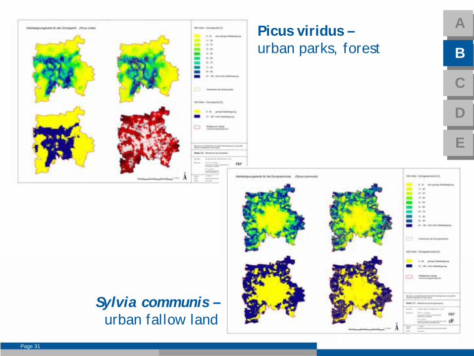
Page 31
Picus viridus – urban parks, forest
Sylvia communis – urban fallow land
A
B
C
D
E

Page 32
Picus viridus
urban green, parks, forest
Model Predictability: 67 -
71 %
Sylvia communis
open/fallow land
A
B
C
D
E
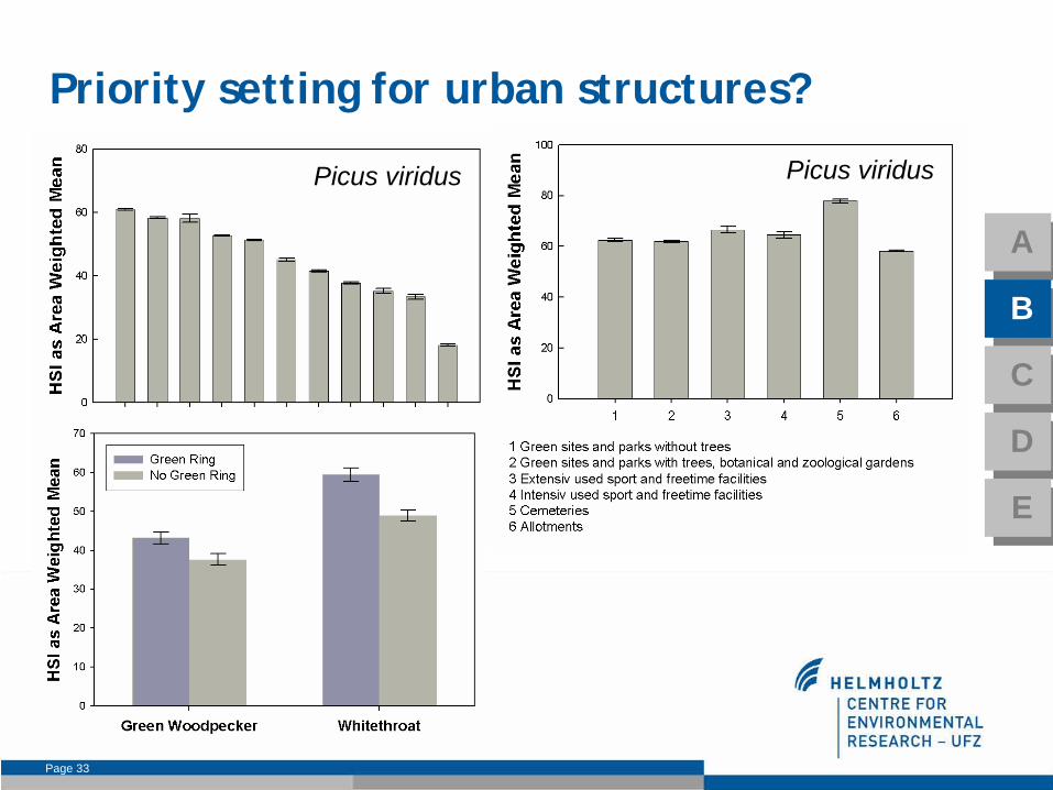
Page 33
Priority setting for urban structures?
Picus viridus Picus viridus
A
B
C
D
E

Page 34
Land use configuration (ED) most important for Green Woodpecker
Habitat requirements of Green Woodpecker and Whitethroat highly contrast; they cover green and brown sites in the city.
ENFA represents a comfortable procedure to quantify habitat preferences for different species using presence data.
Biomapper is suitable tool for the assessment of urban structures and greenery concerning HS.
Advantage for planning purposes: GIS-implementation and visualization as HS-map-series for different scales
Conclusions for Example B
A
B
C
D
E

Page 35
A
B
C
D
E
References
Strohbach, M., Kabisch, N. Haase, D. Birds and the city -
urban biodiversity, land use and social status. Urban Ecosystems.
Page 36
Example C: Does urban sprawl drive changes in
the water balance and policy?
A
B
C
D
E

Page 37
Drivers, Pressures, State, Impact and Response
DriversDrivers
PressuresPressures
StateStateImpactImpact
ResponseResponse
V: demand for urban sprawl depending on demographic and economic dynamics as well as formal (law) and informal (norms, values) institutions
V: land use change from non urban to urban land use
V: land cover and share of
imperviousness
V: water balance in form of sealing rate, groundwater recharge, ETP and surface run-off
V: reactions by authorities and civil society
Target systems
A
B
C
D
E

Page 38
How do ∆ land use and degree of imperviousness impact the urban water balance?
How do we parameterise urban water balance models?
What are the major changes of the urban water balance in the long-term and thus of interestfor landscape planning?
Major questions
A
B
C
D
E

Page 39
Methodology for determining the long-term urban water balance
Effective Evapotranspiration
(employing the Bagrov
relation)
Groundwater recharge (calculated using ABIMO
model 1997)
Runoff regulation (assessment after
MESSER 1997)
Land use (historical and current
topographic maps)
Climate data
(1x1km, DWD*)Grain size, field
capacity (soil maps 1:50.000, 200.000)
Slope
(digital terrain
model
40x40m)
Groundwater level depth (geol. map)
Scanning, geo-
referencing,
digitalisation, error correction
Derivation of model
input
parameters
GIS: Intersection, merge
data
Application
of assessment
tools
Result:
Estimation of the effects of land use, intensification and surfacing on water balance
and surface-runoff
Classifying land use; derivation of degrees of
sealed surfaces (after MÜNCHOW 1999)
Selection of water balance related
processes
Data requirements and stock of data
Data processing
Determining changes to land use and impervious land
A
B
C
D
E

Page 40
Modelling: vertical flow
grain size/
field capacity
groundwater level
potential Evapotranspiration
(ETp)
Precipitation (N)
Direct run-offAO = (N-ETa)*p/100
effective Evapotranspiration
(ETa)Percentage p of
direct run-off
slope
BAGROV-relation
efficiencyparameter n
Groundwater recharge
AU = N-ETa-AO
Land use/
degree of imperviousness
n
p
a
ETET
dPodETa
⎟⎟⎠
⎞⎜⎜⎝
⎛−=1
A
B
C
D
E

Page 41
Mapping urban land use change
Land use classification and mapping
A
B
C
D
E

Page 42
Imperviousness 1870-2003
1870 1940 1985 1997 2003
detailed 6.68 17.06 26.35 29.13 32.19classified 5.74 14.23 22.28 24.63 27.36
% of the total area
0
10
20
30
40
50
60
70
80
90
100
1870 1940 1985 1997 2003
o% im
perv
ious
ness
0
2
4
6
8
10
12
14
16
20-1
00%
impe
rvio
usne
ss
0 20 40
60 80 100
A
B
C
D
E
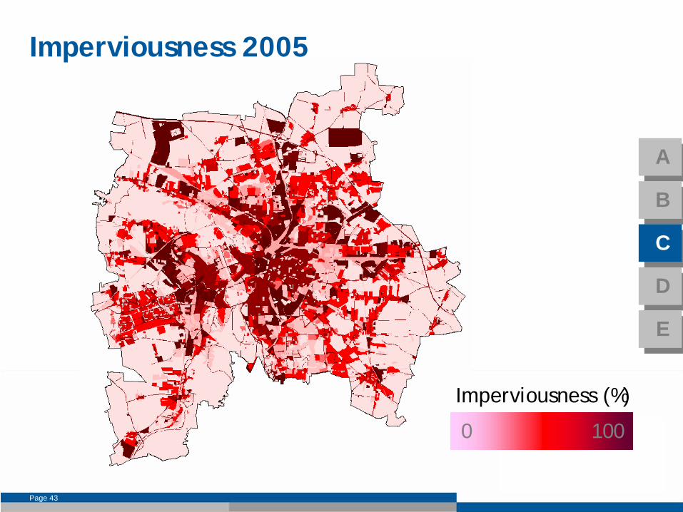
Page 43
Imperviousness 2005
0 100
Imperviousness (%)
A
B
C
D
E

Page 44
Direct runoff 1870 Direct runoff 1985
Direct runoff 1940 Direct runoff 2003
Direct runoff (mm/a)
waters
(Haase, submitted)

Page 45
Recharge rate 1870 Recharge rate 1985
Recharge rate 1940 Recharge rate 2003
Recharge rate (mm/a)
waters
(Haase, submitted)

Page 46
ETP 1870 ETP 1985
ETP 1940 ETP 2003
ETP (mm/a)
waters
(Haase, submitted)

Page 47
Impact of sprawl: ∆
surface run-off and ∆
seeping rate 1985-2003
0
500000
1000000
1500000
2000000
2500000
3000000
1985 2003
Ao
Au
A
B
C
D
E

Page 48
Long-term water balance 1870-2003
Year evapotranspiration [%] (1)
surface run-off [%] (1) seeping water rate [%] (1)
1940 100 100 100
1985 90 154 107
1997 87 170 106
2003 83 262 99
(1) referring to 1940 (1940 = 100 %)
Degree of imperviousness
area evapotrans-
piration
surface run-off seepage water rate
(%) (ha) (mm/a) (mm/a) (mm/a)
> 0 –
20 1111 351 –
550 1 -
150 51 –
300
> 20 –
40 626 251 –
450 51 -
250 51 –
250
> 40 –
60 2547 201 –
350 151 -
300 101 –
200
> 60 –
80 146 151 –
300 251 -
350 51 –
125
> 80 –
100 1842 151 –
200 351 -
450 1 –
75
Water balance of the newly sealed areas in Leipzig since 1940
A
B
C
D
E

Page 49
Vertical and horizontal flow models show effects of land use, ∆ land use and degree of imperviousness on the long-term urban water balance.
There are suitable empirically based parameter sets/functions to parameterise physically based models also for urban areas. Uncertainty assessment is indispensable.
Major changes in the long-term water balance are the decrease of the run-off regulation capacity, an increase of Ao and a respective decrease of ETP which finally leads to a lowering of the water holding capacity of urban area, particularly green spaces and wetlands.
BUT: the study also shows that societal reactions on urban sprawl - first of all the attempts of both authorities and public initiatives to contain sprawl are hardly motivated or influenced by concerns about environmental problems …
… since they are working at the national level (30-ha-goal) and
that the environmental impact of sprawl elicits only indirect repercussions in society.
Conclusions for Example C
A
B
C
D
E

Page 50
A
B
C
D
E
References
Haase, D., Nuissl, H., 2007. Does urban sprawl drive changes in the water balance and policy?
The case of Leipzig (Germany) 1870-
2003. Landscape and Urban Planning 80, 1-13.
Haase, D. Modelling the effects of long-term urban land use change on the urban water balance. Landscape and Environment.
Haase, D. Effects of urbanisation on the water balance –
a long- term trajectory. Environment Impact Assessment Review.

Page 51
Example D: Integrated flood risk analysis and
assessment
A
B
C
D
E

Page 52
Urban floods: the example of Dresden
A
B
C
D
E

Page 53
Urban floods: the example of Dresden
A
B
C
D
E

Page 54
Surface and groundwater level
A
B
C
D
EWater level
at the
gauge
„Augustus bridge“
and the
approximated
values
of a stationary
groundwater
model
Water level
of a groundwater
measuring
station
300 meters
away
(August 2002)
110 110
107107
Page 55
Simulation of the superficial inundation of the city in August 2002 (hazardous flood in the entire Elbe river basin)
Coupling of groundwater, canalisation and surface water flows to determine mutual impacts
Scenario quantification
Major questions:
A
B
C
D
E

Page 56
Approach 3ZM-GRIMEX
A
B
C
D
E

Page 57
Task UFZ: Inundation modelling
A
B
C
D
E
Channel model
Groundwater model

Page 58
DataData set Type Source Spatio-temporal
resolution
DEM Raster Environmental Agency Dresden 1 x 1m
DEM Raster Environmental Agency Dresden 50 x 50m
Valley bottom
topography Vector LVM Sachsen 2.5 –
20m
Buildings Vector Environmental Agency Dresden 1:10.000
Land use Vector Environmental Agency Dresden 1:10.000
Streamflow
of the
river
Elbe at different gauges
Time series Water board
Dresden (WSA DD) 01.01.2002 . 01.01.200415 minutes
interval
01.03.2006 -
15.05.200615 minutes
interval
Streamflow
of the
creeks
Müglitz, Weißeritz, Lockwitzbach
Time series Saxon
State Agency for
Geology
and Environment
01.08.2002 . 31.10.20021h intervall
Assigned
flooding
areas
(not
legally
binding)Vector Saxon State Agency for Geology
and Environment1 : 100,000
Legally
binding
flood
risk
zones Vector Environmental Agency Dresden 1 :10,000
Flooded
areas(detected
at 17.08.2002)Vector Environmental Agency Dresden 1 :10,000
Flooding
areas
based
on stationary
modelVector Environmental Agency Dresden 1 : 25,000
Dams Vector Environmental Agency Dresden 1 : 10,000
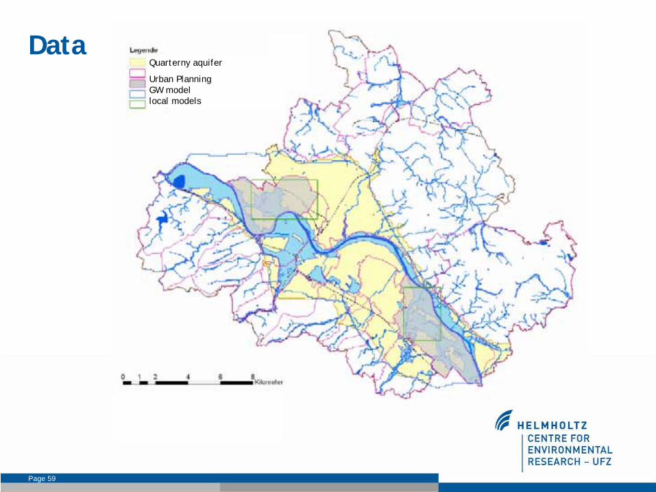
Page 59
DataQuarterny aquifer
Urban Planning
GW model
local
models

Page 60
Topography data
Elbe -
Laser-DGM (1x1m) Elbe -
DGM-W Elbe-South (5x5m)
Laser-DGM (1x1m) without buildungs Laser-DGM (1x1m) with buildings
A
B
C
D
E

Page 61
Topographic and Land Use Data
A
B
C
D
E

Page 62
Logic of water flow coupling
A
B
C
D
E

Page 63
Logic of water flow coupling
surface, channel
groundwater
A
B
C
D
E

Page 64
Logic of water flow coupling (2)
Definition of the coupling timing
Water Level of the Elbe
A
B
C
D
E

Page 66
Inundation modelling 2D (space)
Maximum flooding
(flood
2002) using
surface
roughness
Manning‘s
of 0.2
Maximum flooding
(flood
2002) using
surface
roughness
Manning‘s
of
0.02
A
B
C
D
E
Page 67
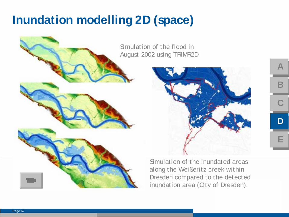
Inundation modelling 2D (space)
Simulation of the flood in August 2002 using TRIMR2D
Simulation of the inundated areas along the Weißeritz
creek within Dresden compared to the detected inundation area (City of Dresden).
A
B
C
D
E

Page 68
Inundation modelling 2D (time)
A
B
C
D
E

Page 69
Inundation modelling 2D (time)
103
105
107
109
111
113
115
Pegel m ü. NN diff_tudd 0022_004 0022_02 0022_002 004all
Page 70
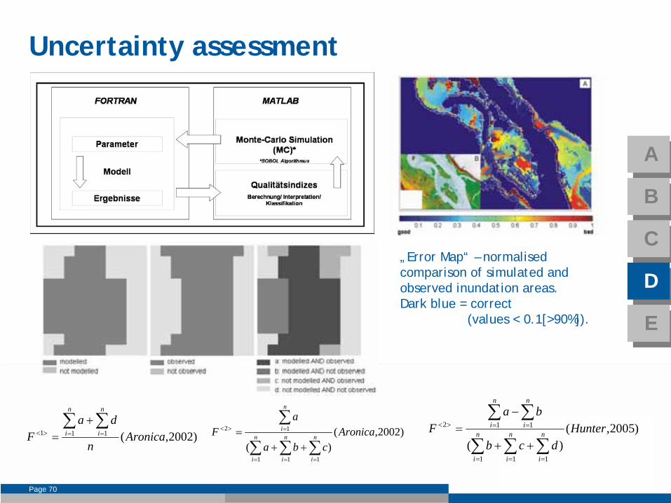
Uncertainty assessment
„Error Map“
–
normalised comparison of simulated and observed inundation areas. Dark blue = correct
(values < 0.1[>90%]).
)2002,(111 Aronican
daF
n
i
n
i∑∑==><
+= )2002,(
)(111
12 Aronicacba
aF n
i
n
i
n
i
n
i
∑∑∑
∑
===
=><
++= )2005,(
)(111
112 Hunterdcb
baF n
i
n
i
n
i
n
i
n
i
∑∑∑
∑∑
===
==><
++
−=
A
B
C
D
E

Page 71
Impacts of groundwater flows
surface
canalisation
groundwater
A
B
C
D
E

Page 72
Impacts of groundwater flows
Simulation using TrimR2D Groundwater reaction PCGEOFIM
A
B
C
D
E
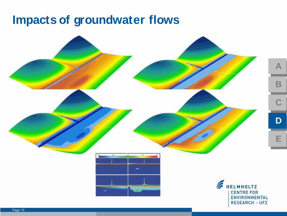
Page 73
Impacts of groundwater flows
A
B
C
D
E

Page 74
WebGIS
“Mulde flood”
A
B
C
D
E
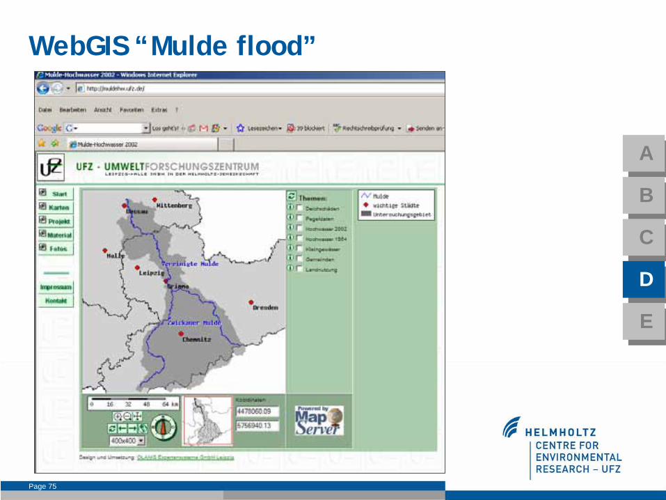
Page 75
WebGIS
“Mulde flood”
A
B
C
D
E

Page 76
WebGIS
“Mulde flood”
A
B
C
D
E

Page 77
WebGIS
“Mulde flood”
A
B
C
D
E
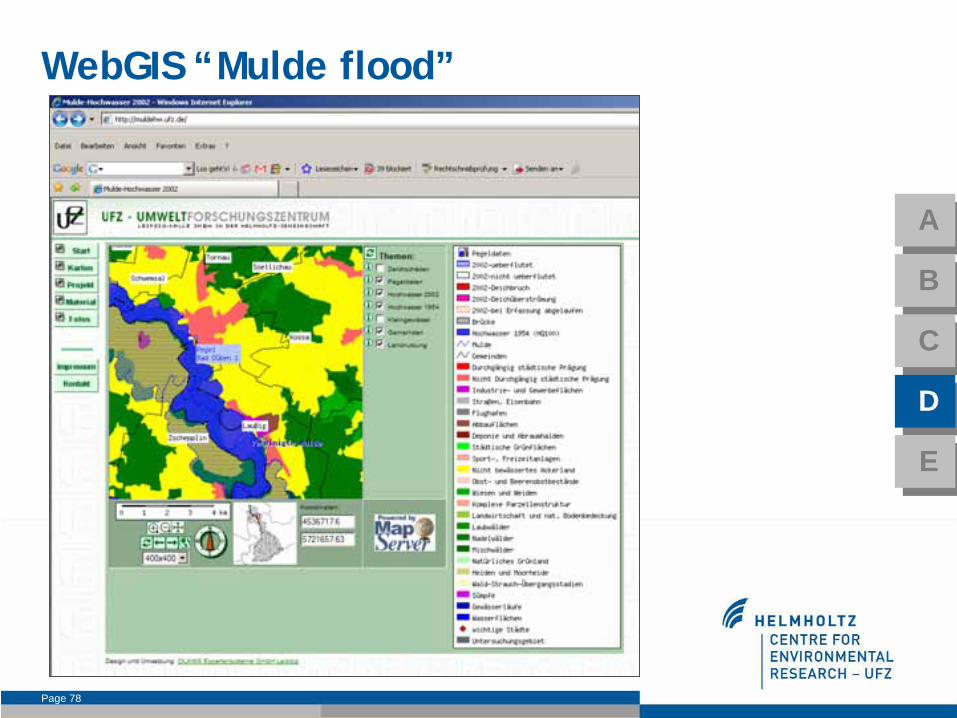
Page 78
WebGIS
“Mulde flood”
A
B
C
D
E
Page 79
A
B
C
D
E
References
Meyer, V., Scheuer, S., Haase, D. 2008. A multi-criteria approach for flood risk mapping exemplified at the Mulde river, Germany. Natural Hazards, DOI: 10.1007/s11069-008-9244-4.
Haase, D., Weichel, T. & M. Volk (2003). Approaches towards the analysis and assessment of the disastrous floods in Germany in August 2002 and consequences for land use and retention areas.
Vaishar, A., Zapletalova, J. & J. Munzar
(eds.): Regional Geography and its Applications, proceedings of the 5th Moravian Geographical Conference CONGEO'03, 51-59.

Page 80
Example E: GIS and model based analysis of
historical land use change as base for recent planning
A
B
C
D
E

Page 81
Landscape change
Hypothesis: How have land use and landscape structure changed over historical periods along the rural-urban gradient?
How have these changes to the landscape affected the ecosystem pattern and biophysical processes, particularly water and nutrient fluxes as well as biodiversity (as services provided by landscapes)?
Can general trends be concluded regarding future changes to land use and its structuring over the next decades?

Page 82
Local/regional land use change
Land use transition matrix
aggregation
detection
Land development history/scenarios
interpretation
Conceptual model and scales
Haase et al., 2007
A
B
C
D
E

Page 83
Equidistant Map 1879 Survey Map 1927 Top. Map TK25 1997
Digital land use data sets
Georeferencing and editing of land use classes
Final data set
Overlaying polygons
Splitting polygons
class definition
class correction
analogue digital
GIS
Bringing historical maps into GIS
Haase et al., 2007

Page 84
Regulation Function
(ecosystem service)
Land usetopographic
map 1:25.000
Soil indicessoil maps 1:25.000
and 1:200.000
ClimateDWD* 1x1km
raster
TopographyDigital Terrain Model 25x25m
Land usetopographic
map 1:25.000
Soil indicessoil maps 1:25.000
and 1:200.000
ClimateDWD* 1x1km
raster
TopographyDigital Terrain Model 25x25m
Ground Water Recharge
Model ABIMO (Glugla & Fürtig, 1997)
Run-off regulation
Marks et al. (1992)
Erosion ResistanceFunction
Marks et al. (1992)
Ground Water Recharge
Model ABIMO (Glugla & Fürtig, 1997)
Run-off regulation
Marks et al. (1992)
Erosion ResistanceFunction
Marks et al. (1992)
Land useclasses
Grain sizeGroundwater level
Field capacity precipitationevapotranspir.
slopecurvature
Land useclasses
Grain sizeGroundwater level
Field capacity precipitationevapotranspir.
slopecurvature
Land useclasses
Grain sizeGroundwater level
Field capacity precipitationevapotranspir.
slopecurvature
Landscape functions analysis
Haase et al., 2007
A
B
C
D
E
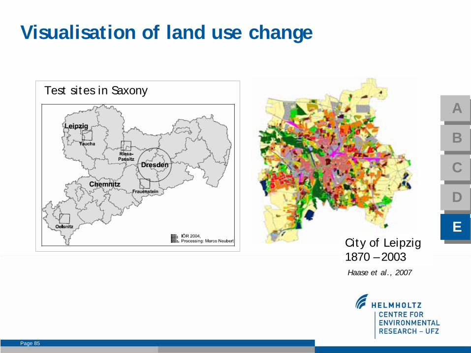
Page 85
City of Leipzig 1870 –
2003
Visualisation of land use change
Haase et al., 2007
Test sites in Saxony
A
B
C
D
E
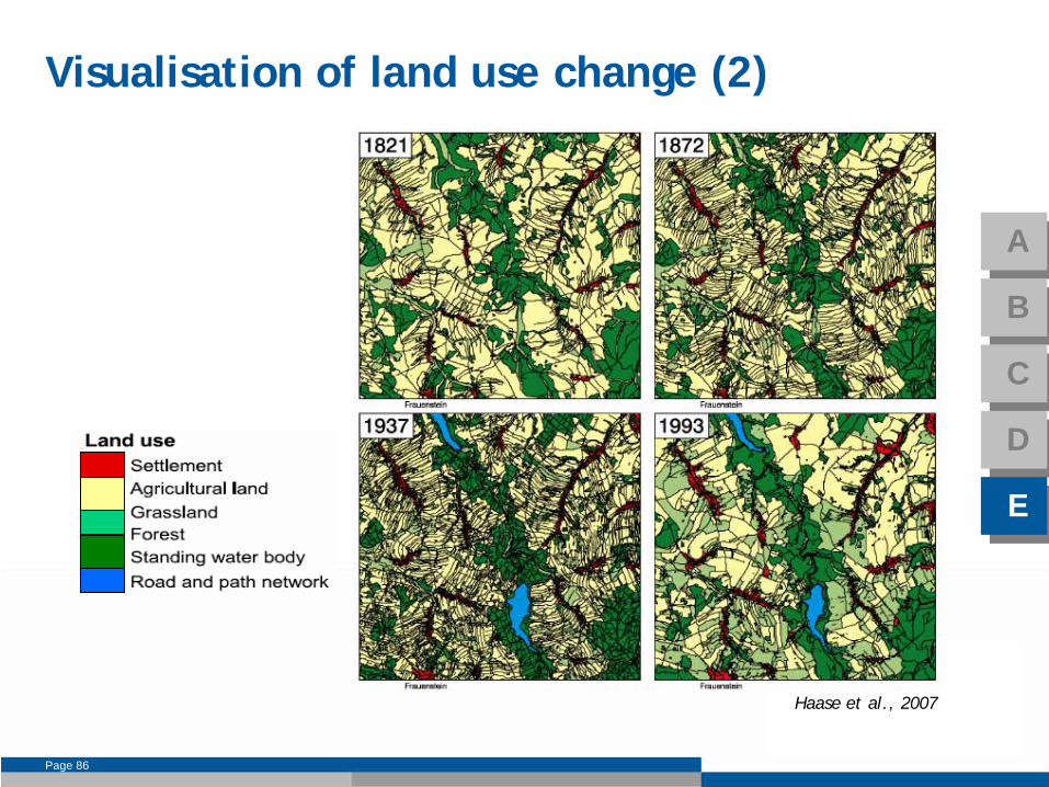
Page 86
Visualisation of land use change (2)
Haase et al., 2007
A
B
C
D
E

Page 87
Changes of the landscape structure
Haase et al., 2007
A
B
C
D
E

Page 88
City of Dresden 1880-1998
Quantification of land use change
Haase et al., 2007

Page 89
year Ground water recharge rate (mm)
1-25 26-50 51-75 76-100 101-150 151-200 201-250
1879 9 8 18 17 35 13 0
1927 9 9 19 17 31 14 1
1997 10 12 23 21 24 8 0
1927 1997
Change of landscape functionality 1879
Haase et al., 2007

Page 90
Landscape and Land Use Change in a lignite mining area south to Leipzig:
Future landscape concepts are based on historical data and planners’ ideas.
Future Land Use Change in the Tisza River Basin due to Global Change.
Haase et al., 2007
Using the history for shaping the future

Page 91
Historical maps can be integrated into a GIS to model/show land use change quantitatively over >200 years.
Statistics can then be compiled on the development of the proportions of linear elements and areas of certain usage types.
Interpretation and future planning of landscape development can be quantitatively substantiated.
Taking into account landscape functions in the assessment brings home how important it is to consider the ‘loss’ of not only land in the meaning of total area but also resources.
Quantification of long-term land use change and its environmental impact enables us to reduce the existing uncertainty to predict future landscape change in land use change or biophysical models which often limits planning.
Conclusions for Example D
A
B
C
D
E

Page 92
A
B
C
D
E
References
Haase, D., Nuissl, H., 2007. Does urban sprawl drive changes in the water balance and policy?
The case of Leipzig (Germany) 1870-
2003. Landscape and Urban Planning 80, 1-13.
Haase, D., Walz, U., Neubert, M., Rosenberg, M. 2007. Changes to Saxon landscapes -
analysing historical maps to approach current
environmental issues. Land Use Policy 24, 248-263.

Page 93
Main questions raised are in close connection to what concerns landscape change and resource planning or management.
The items touched come from different fields of landscape ecology and thus comprise different components and variables of the landscape in space and time.
Models and GIS had been presented as a kind of relational and mutually feeding methodologies that support applied research andprovide planning and land use policy with quantitative tools.
At the UFZ we recently incorporate agent behavior and heuristics of decision-making as a key to better understand land use changes (ABM, role games).
Synthesis

Page 94
Thank you for the attention.