the use of - ajbasweb.comajbasweb.com/old/ajbas/2010/1221-1239.pdf · the use of finite difference...
TRANSCRIPT
Australian Journal of Basic and Applied Sciences, 4(6): 1221-1239, 2010ISSN 1991-8178
The Use of Finite Difference Method, Homotopy Perturbation Method andVariational Iteration Method for a Special Type of Linear Fredholm
Integro-differential Equations
1B. Raftari, 2A. Ahmadi, 3H. Adibi
1Department of Mathematics, Islamic Azad University, Kermanshah branch, P.C. 6718997551, Kermanshah, Iran
2Department of Physics, Islamic Azad University, Malayer branch, Malayer, Iran3Department of Mathematics and Computer Science,
Amirkabir University of Technology, No. 424, Hafez Ave., Tehran, Iran
Abstract: Special type of linear Fredholm integro-differential equations is considered. In this research,two analytical methods, called homotopy-perturbation method (HPM) and variational iteration method(VIM) and one numerical method, finite difference method are used for solving these equations. Theresults of applying these methods to the linear integro-differential equation show the simplicity andefficiency of these methods.
Key words: Fredholm integro-differential equations; Homotopy perturbation method; finite differencemethod; Variational iteration method
INTRODUCTION
Mathematical modeling of real-life problems usually results in functional equations, e.g. partial differentialequations, integral and integro-differential equation, stochastic equations and others. Many mathematicalformulation of physical phenomena contain integro-differential equations, these equations arises in fluiddynamics, biological models and chemical kinetics; for more detail see (Kythe, P.K., P. Puri, 2002; Wazwaz,A.M., 2006) and the references cited therein. Integro-differential equations are usually difficult to solveanalytically so it is required to obtain an efficient approximate solution. VIM is to construct correctionfunctional using general Lagrange multipliers identified optimally via the variational theory, and the initialapproximations can be freely chosen with unknown constants. This method is the most effective and convenientone for both linear and nonlinear equations. This method has been shown to effectively, easily and accuratelysolve a large class of linear and nonlinear problems with components converging rapidly to accurate solutions.VIM was first proposed by He (1999) and was successfully applied to various engineering problems (He, J.H.,2000; Momani, Sh., S. Abuasad, 2006; Ganji, D.D., A. Sadighi, 2007). HPM is also a straightforward andconvenient method for both linear and nonlinear equations. This method does not depend on a small parameter.Using homotopy technique in topology, a homotopy is constructed with an embedding parameter p � [0,1],which is considered as a “small parameter” (He, J.H., 2000; He, J.H., 2006; He, J.H., 2003; He, J.H., 2006;He, J.H., 2005). The HPM deforms a difficult problem into a simple problem which can be easily solved. Thefinite difference method, based upon Simpson rule and numerical differentiation, transforms the Fredholmintegro-differential equation into a matrix equation.
In this study, we apply these methods to solve the following linear Fredholm integro-differential equation
(1)� � � � � � � � � � � �� �
, , ,
0
bu x x u x f x k x t u t dt a x bau a u
� �� � � � ��
��
where the functions f(x), �(x) and the kernel k(x,t) are known and u(x) is the solution to be determined.
Corresponding Author: B. Raftari, Department of Mathematics, Islamic Azad University, Kermanshah branch, P.C.6718997551, Kermanshah, Iran E-mail: [email protected]
1221

Aust. J. Basic & Appl. Sci., 4(6): 1221-1239, 2010
2. Finite Difference Method:In this section, we consider Fredholm integro-differential equation in (1) and approximate to solution by
numerical integration and numerical differentiation. We will subdivide the interval of integration (a,b) into
N = 2M equal subinterval of width . Since we will be using either t or x as the , 1b ah NN�
�
independent variable, therefore let and . We will refer to the value of the x a ih ti i � � �f x fi i
functions and at as and , and the approximate � �,k x t � �x� xi � �,k x t ki j ij � �xi i� �
value of the solution and at as and . So if we use the � �u x � �u x� xi � �u x ui i � �u x ui i� �
Simpson rule to approximate the integral in the integro-differential equation (1), we have
� � � �� � � � � � � � � � � �
� � � � � � � �, 4 , 2 , ...0 0 1 1 2 2, ,
3 4 , ,1 1
k x t u t k x t u t k x t u thb k x t u t dta k x t u t k x t u tN N N N
� �� � �� ��� � �� �� �� �� �
Also the integro-differential equation (1) is approximated by
� � � � � � � �� � � � � � � � � � � �
� � � � � � � �, 4 , 2 ,0 0 1 1 2 2 ,
3 ... 4 , ,1 1
k x t u t k x t u t k x t u thu x x u x f xk x t u t k x t u tN N N N
�� �� �� �� � �� �� � �� �� �� �
and
� � � � � � � �
� � � � � � � � � � � �� � � � � � � �
, 4 , 2 ,0 0 1 1 2 2 , 1, 2,..., .3 ... 4 , ,1 1
u x x u x f xi i i
k x t u t k x t u t k x t u th i i i i Nk x t u t k x t u ti N N i N N
�� �
� �� �� �� � �� � �� �� �� �
(2)
and accordingly the system of equations (2) can be written in the following more compact form
4 2 ...0 0 1 1 2 2 , 1,2,..., .43 , 1 1
k u k u k uh i i iu u f i Ni i i i k u k ui N N iN N
��� � �� �
� � �� � � �� �� �� �
Now we take advantage of finite differentiation to get
(3)
4 2 ...0 0 1 1 2 21 1 ,42 3 , 1 1
1,2,..., 1,
k u k u k uu u h i i ii i u fi i i k u k uh i N N iN Ni N
��� � �� ��� � � �� �
� �� �� �� � �
1222

Aust. J. Basic & Appl. Sci., 4(6): 1221-1239, 2010
and
(4)
3 4 1 22
4 2 ...0 0 1 1 2 2 ,43 , 1 1
u u uN N N u fN N Nhk u k u k uh N N N
k u k uN N N NN N
�
�
� �� � �
� � �� �� ��� �� �� �� �
as a system consisting N equations which by virtue of (3) and (4) can be written in the following matrix form
KU F
where
2 2 2 2 28 4 8 4 22 1 ...11 1 12 13 14 13 3 3 3 3
2 2 2 2 28 4 8 4 21 2 1 ...21 22 2 23 24 23 3 3 3 3
2 2 28 4 81 231 32 33 33 3 3
h h h h hk h k k k k N
h h h h hk k h k k k N
h h hk k k h
K
� � � � ��
� � � � ��
� � � �
� � � �� � � �� � � � � � �� � � �� � � �� � � � � �� � � � � �� � � � � � � �� � � � � �� � � � � �
� � �� � �� � � � �� � �� � �
2 28 21 ...34 23 3
. . . . . . .
. . . . . . .
. . . . . . .2 2 2 2 28 8 4 8 8... 1 2 11,1 1, 3 1, 2 1, 13 3 343 3 3 3 3
2 2 28 8 4... 11 , 3 , 23 3 3
h hk k N
h h h h hk k k k h kN N N N N N N
h h hk k kN N N N N
� �
� � � � ��
� � �
� � �� � �� � �� � �� � �
� � � � � �� � � � � �� � � � � � � �� � � � � � �� � � � � �� � � � � �
� ��� � � �� ��� �
2 28 24 3 2, 13 3h hk k hN N NN N
� � �
� �� �� �� �� �� �� �� �� �� �� �� �� �� �� �� �� �� �� �� �� �� �� � � �� �� � � � �� � � � ��� �� � � � �
� � � �� �
1
2
.
.
.
N
uu
U
u
� �� �� �� �
� �� �� �� �� �� �
and
1223
Aust. J. Basic & Appl. Sci., 4(6): 1221-1239, 2010
222 11 10 03
222 2 20 03222 3 30 03222 2 40 03
.
.
.222 1 1,0 03
222 0 03
.
hhf k u
hhf k u
hhf k u
hhf k u
F
hhf k uN N
hhf k uN N
�
�
�
�
�
�
� �� �� �� �� �
� �� �� �� �� �� ��� �� �� ��� �� �� �
�� �� �
� �� �� �� �� �� �
�� �� �� �� �� ��� �� �� �� �� �� �
2. Homotopy Perturbation Method:To illustrate the basic ideas of the homotopy perturbation method, we consider the following nonlinear
differential equation:
(5)( ) ( ) 0,A u f r r� ��
with the boundary conditions
(6), 0,uB u rn
� � ��� � � �
where A is a general differential operator, B is a boundary operator, f(r) is a known analytical functionand � is the boundary of the domain �. Generally speaking, operator A can be divided into two parts whichare L and N where L is linear, but N is nonlinear. Therefore equation (5) can be rewritten as follows:
(7)� � � � � � 0.L u N u f r� �
By the homotopy perturbation technique, we construct a homotopy which satisfies:� � ! ", : 0,1v r p R�# $
(8)� � � � � � � � � � � � ! ", 1 0, 0,1 , ,0H v p p L v L u p A v f r p r� � � � � � � ��� �� �� �
Where p �[0,1] is an embedding parameter and uo is an initial approximation of equation (1).Obviously,from these definitions we will have:
� � � � � � � � � � � �0,0 0, ,1 0.H v L v L u H v A v f r � �
1224

Aust. J. Basic & Appl. Sci., 4(6): 1221-1239, 2010
The changing process of p from zero to one is just that of v(r,p) from uo(r) to (r).In topology, this iscalled deformation, and L(v) - L (uo), and A(v)-f(r) are called homotopy. According to the HPM, we can firstuse the embedding parameter p as a “small parameter”, and assuming that the solution of (8) can be writtenas a power series in p:
(9)20 1 2 ... .v v pv p v � � �
Setting p=1, results in the approximate solution of (5):
0 1 21lim ... .p
u v v v v$
� � �
In order to solve the equation (1) using HPM, we construct the following homotopy:
(10)
� � � � � � � �� �� � � � � � � � � � � �� �
, 1
, 0.b
a
H v p p v x f x
p v x x v x k x t v t dt f x� �
� � �
�� � � � �Substituting (9) in (10) and equating the coefficients of like powers of p yields:
(11)� � � � � �00 0 0: 0,p v x f x v a u� �
(12)� � � � � � � � � � � � � �11 1: , 0, 0, 1
b
n n n nap v x x v x k x t v t dt v a n� �� �� � � ��
We can identify vn for n = 0, 1,2.... and therefore, we obtain the n-th approximation of the exact solutionas 0 1 ... .n nu v v v � � �
3. Variational Iteration Method:To illustrate the basic concepts of the variational iteration method (He J.H., 1999), we consider the
following differential equation:
(13)� � � � � � ,L u N u g x�
where L is a linear operator, N is a nonlinear operator, and g(x,i) is an inhomogeneous term. Then we canconstruct a correct functional as follows:
(14)� � � � � � � � � � � �� �� �% &1 0,
t
n n n nu x u x s L u s N u s g s ds�� � � �� �
where � is a general Lagrange multiplier (He, J.H., 1999; He, J.H., 2000; Momani, Sh., S. Abuasad, 2006),which can be identified optimally via variational theory.
The second term on the right is called the correction and is considered as a restricted variation,nu�i.e. 0.nu' �
With the determination of �, the approximations follow immediately. Consequently,� � � �, 0nu x t n �the exact solution may be obtained by using
� � � �lim .nnu x u x
$(
We consider the equation (1). According to the variational iteration method, we can construct the followingcorrect functional:
1225

Aust. J. Basic & Appl. Sci., 4(6): 1221-1239, 2010
(15)
� � � �
� � � � � � � � � � � � � �% &1
0, ,
n n
t b
n n na
u x u x
s u s s u s f s k s t u t dt ds� � �
�
�� � � �� �� �
where is considered as a restricted variation, i.e. , and � is the general Lagrangenu' � 0nu' �multiplier.
Making the above correct functional stationary, and noticing that 0,nu' �
(16)� � � � � � � � � � � � � � � � � �% &
� � � � � � � � � �
1 0
0
,
| ,
t b
n n n n na
t
n n s x n
u x u x s u s s u s f s k s t u t dt ds
u x s u s s u s ds
' ' ' � � �
' � ' � '
�
� � � � �
� � �
� �
�
� �
which yields the following stationary conditions
� �� �
1 0,
0.
s
s
�
�
�
�
Therefore, the general Lagrange multiplier can be readily identified as:
� � 1.s� �
Substituting this value of the Lagrangian multiplier into functional (15) gives the iteration formula
(17)� � � � � � � � � � � � � � � � � �% &1 0, ,
t b
n n n n nau x u x s u s s u s f s k s t u t dt ds� � �� � � � � �� �
Now we begin with an initial approximation by the above iteration formula,� � � �0 0 ,u x u a u we can obtain the � � for 1.nu x �
4. Illustrative Examples: Now we apply the methods presented to solve the following examples:
Example 1: (Rashidinia, J., M. Zarebnia, 2007)Consider the Fredholm integro-differential equation:
� � � � � �� �
� �
� �
1
2 0
1 1 1ln 1 , 0 1,2 1 1ln 2
0 0
xu x u x x x u t dt xx t
u
� � � � � � � � � � � � �
�
which has the exact solution . The numerical results are represented in Table 1 and� � � �ln 1u x x �Figures 1-8.
Example 2: (Rashidinia, J., M. Zarebnia, 2007)As the second example consider the Fredholm integro-differential equation:
1226

Aust. J. Basic & Appl. Sci., 4(6): 1221-1239, 2010
� � � � � � � �
� � � � � �
� �
1
0
cos 2 2 sin 21 sin 4 sin 4 2 , 0 1,2
0 1
u x u x x x
x x t u t dt x
u
) ) )
) ) )
�� � � ��� � � � �� �
�
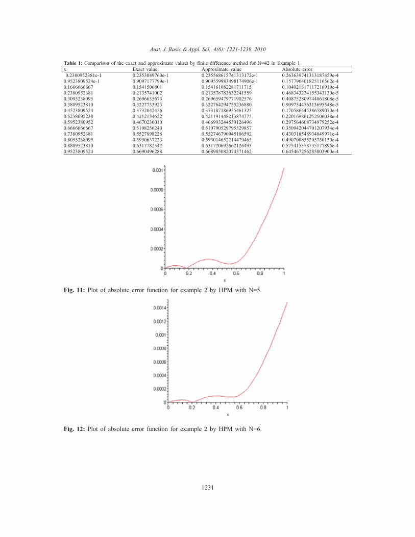
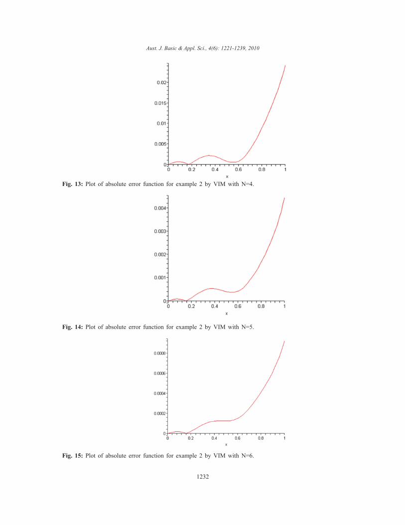
With the exact solution . Table 2 and Figures 9-16 illustrate the numerical results. � � � �cos 2u x x)
Example 3: (New Jersey, 1997)Consider []
� � � �� �
1
0, 0 1,
0 0
x tu x x e u t dt x
u
�� � � �
��
�
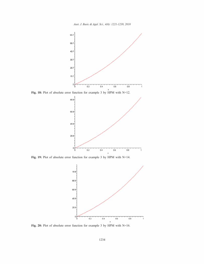
With the exact solution Results are shown in Table 3 and� �2 2 5 2 5 .
2 2 2 2 2xx e eu x e
e e� �� � � � � �� � � �� �� � � �Figures 17-24.
Example 4: (New Jersey, 1997)At last, we consider
� � � � � �
� �
11
0
1 1sinh 1 , 0 1,8 8
0 1
u x x e x xtu t dt x
u
�� � � � � � � �
�
which has the exact solution . Table 2 and Figures 25-32 illustrate the numerical results. � � coshu x x
Fig. 1: Plot of absolute error function for example 1 by HPM with N=6.
1227

Aust. J. Basic & Appl. Sci., 4(6): 1221-1239, 2010
Fig. 2: Plot of absolute error function for example 1 by HPM with N=8.
Fig. 3: Plot of absolute error function for example 1 by HPM with N=10.
Fig. 4: Plot of absolute error function for example 1 by HPM with N=12.
1228
Aust. J. Basic & Appl. Sci., 4(6): 1221-1239, 2010
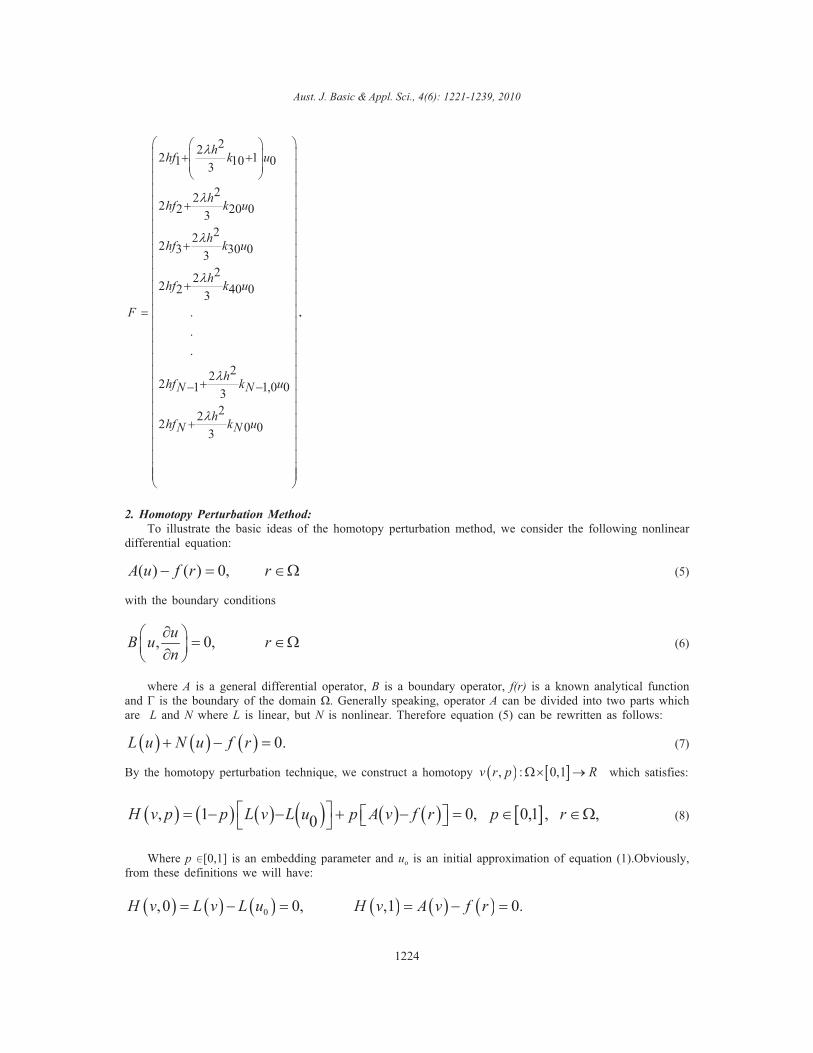
Fig. 5: Plot of absolute error function for example 1 by VIM with N=6.
Fig. 6: Plot of absolute error function for example 1 by VIM with N=7.
Fig. 7: Plot of absolute error function for example 1 by VIM with N=8.
1229
Aust. J. Basic & Appl. Sci., 4(6): 1221-1239, 2010
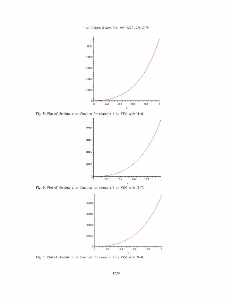
Fig. 8: Plot of absolute error function for example 1 by VIM with N=9.
Fig. 9: Plot of absolute error function for example 2 by HPM with N=3.
Fig. 10: Plot of absolute error function for example 2 by HPM with N=4.
1230
Aust. J. Basic & Appl. Sci., 4(6): 1221-1239, 2010
Table 1: Comparison of the exact and approximate values by finite difference method for N=42 in Example 1x Exact value Approximate value Absolute error 0.2380952381e-1 0.2353049760e-1 0.235568615741313172e-1 0.263639741313187459e-40.9523809524e-1 0.9097177799e-1 0.909559983498174906e-1 0.157796401825116562e-40.1666666667 0.1541506801 0.154161082281711715 0.104021817117216919e-40.2380952381 0.2135741002 0.213578783632241559 0.468343224155343130e-50.3095238095 0.2696635673 0.269659479771902576 0.408752809744061808e-50.3809523810 0.3227733923 0.322764294755236880 0.909754476313695548e-50.4523809524 0.3732042456 0.373187186955461325 0.170586445386589070e-40.5238095238 0.4212134652 0.421191448213874775 0.220169861252506038e-40.5952380952 0.4670230010 0.466993244539126496 0.297564608734979252e-40.6666666667 0.5108256240 0.510790529795529857 0.350942044701207934e-40.7380952381 0.5527898228 0.552746790945106592 0.430318548934049971e-40.8095238095 0.5930637223 0.593014652214479465 0.490700855205750130e-40.8809523810 0.6317782342 0.631720692662126493 0.575415378735177896e-40.9523809524 0.6690496288 0.668985082074371462 0.645467256285003900e-4
Fig. 11: Plot of absolute error function for example 2 by HPM with N=5.
Fig. 12: Plot of absolute error function for example 2 by HPM with N=6.
1231
Aust. J. Basic & Appl. Sci., 4(6): 1221-1239, 2010
Fig. 13: Plot of absolute error function for example 2 by VIM with N=4.
Fig. 14: Plot of absolute error function for example 2 by VIM with N=5.
Fig. 15: Plot of absolute error function for example 2 by VIM with N=6.
1232
Aust. J. Basic & Appl. Sci., 4(6): 1221-1239, 2010
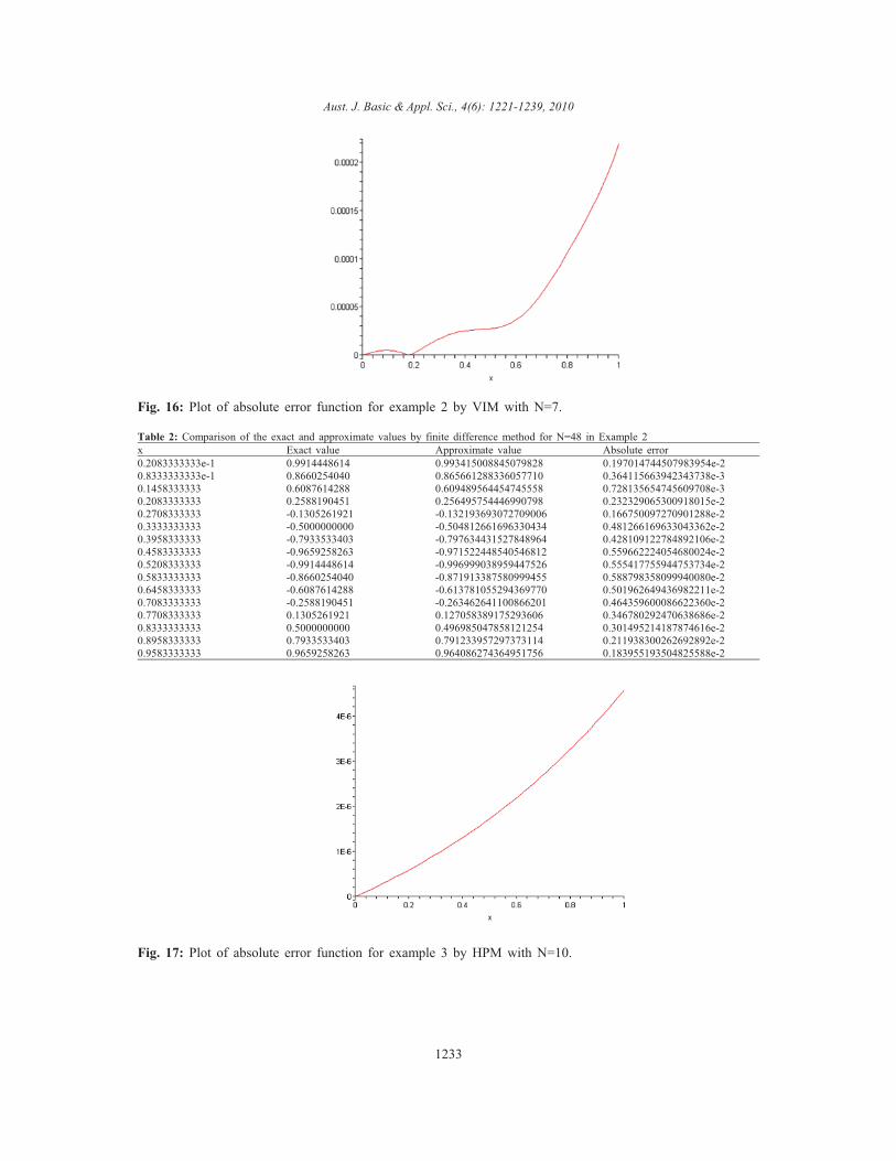
Fig. 16: Plot of absolute error function for example 2 by VIM with N=7.
Table 2: Comparison of the exact and approximate values by finite difference method for N=48 in Example 2x Exact value Approximate value Absolute error0.2083333333e-1 0.9914448614 0.993415008845079828 0.197014744507983954e-2 0.8333333333e-1 0.8660254040 0.865661288336057710 0.364115663942343738e-30.1458333333 0.6087614288 0.609489564454745558 0.728135654745609708e-30.2083333333 0.2588190451 0.256495754446990798 0.232329065300918015e-20.2708333333 -0.1305261921 -0.132193693072709006 0.166750097270901288e-20.3333333333 -0.5000000000 -0.504812661696330434 0.481266169633043362e-20.3958333333 -0.7933533403 -0.797634431527848964 0.428109122784892106e-20.4583333333 -0.9659258263 -0.971522448540546812 0.559662224054680024e-20.5208333333 -0.9914448614 -0.996999038959447526 0.555417755944753734e-20.5833333333 -0.8660254040 -0.871913387580999455 0.588798358099940080e-20.6458333333 -0.6087614288 -0.613781055294369770 0.501962649436982211e-20.7083333333 -0.2588190451 -0.263462641100866201 0.464359600086622360e-20.7708333333 0.1305261921 0.127058389175293606 0.346780292470638686e-20.8333333333 0.5000000000 0.496985047858121254 0.301495214187874616e-20.8958333333 0.7933533403 0.791233957297373114 0.211938300262692892e-20.9583333333 0.9659258263 0.964086274364951756 0.183955193504825588e-2
Fig. 17: Plot of absolute error function for example 3 by HPM with N=10.
1233
Aust. J. Basic & Appl. Sci., 4(6): 1221-1239, 2010
Fig. 18: Plot of absolute error function for example 3 by HPM with N=12.
Fig. 19: Plot of absolute error function for example 3 by HPM with N=14.
Fig. 20: Plot of absolute error function for example 3 by HPM with N=16.
1234
Aust. J. Basic & Appl. Sci., 4(6): 1221-1239, 2010
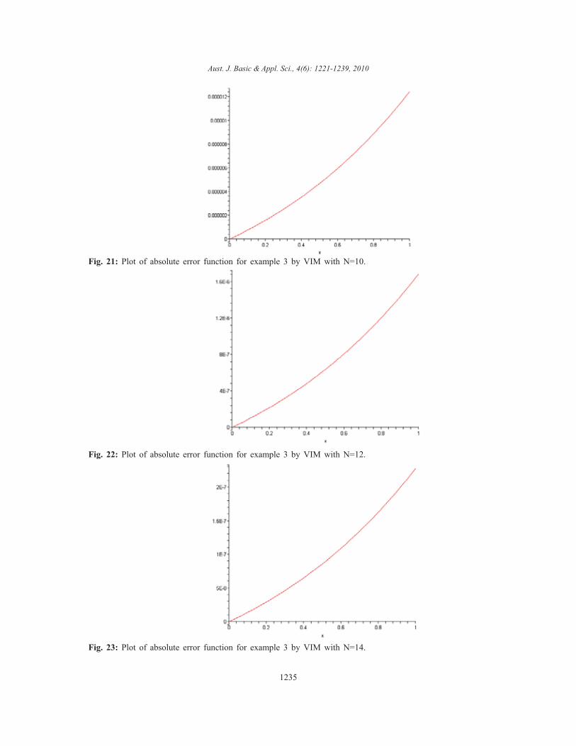
Fig. 21: Plot of absolute error function for example 3 by VIM with N=10.
Fig. 22: Plot of absolute error function for example 3 by VIM with N=12.
Fig. 23: Plot of absolute error function for example 3 by VIM with N=14.
1235
Aust. J. Basic & Appl. Sci., 4(6): 1221-1239, 2010
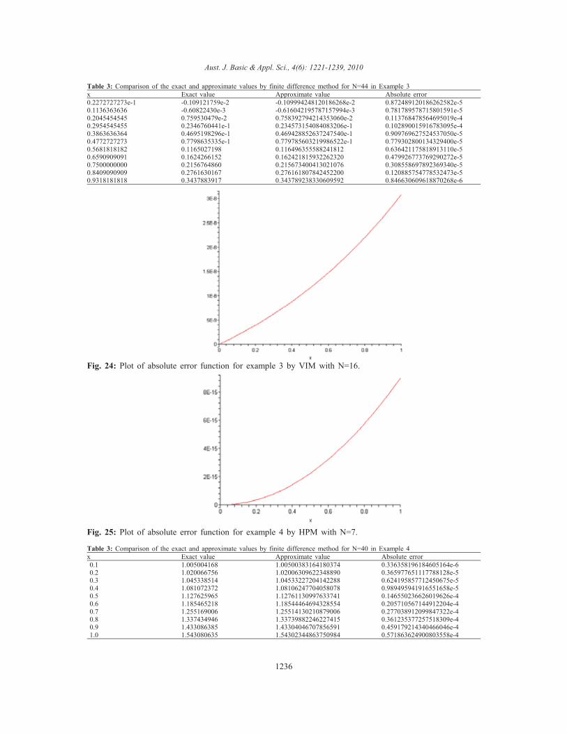
Table 3: Comparison of the exact and approximate values by finite difference method for N=44 in Example 3x Exact value Approximate value Absolute error0.2272727273e-1 -0.109121759e-2 -0.109994248120186268e-2 0.872489120186262582e-50.1136363636 -0.60822430e-3 -0.616042195787157994e-3 0.781789578715801591e-50.2045454545 0.759530479e-2 0.758392794214353060e-2 0.113768478564695019e-40.2954545455 0.2346760441e-1 0.234573154084083206e-1 0.102890015916783095e-40.3863636364 0.4695198296e-1 0.469428852637247540e-1 0.909769627524537050e-50.4772727273 0.7798635335e-1 0.779785603219986522e-1 0.779302800134329400e-50.5681818182 0.1165027198 0.116496355588241812 0.636421175818913110e-50.6590909091 0.1624266152 0.162421815932262320 0.479926773769290272e-50.7500000000 0.2156764860 0.215673400413021076 0.308558697892369340e-50.8409090909 0.2761630167 0.276161807842452200 0.120885754778532473e-50.9318181818 0.3437883917 0.343789238330609592 0.846630609618870268e-6
Fig. 24: Plot of absolute error function for example 3 by VIM with N=16.
Fig. 25: Plot of absolute error function for example 4 by HPM with N=7.
Table 3: Comparison of the exact and approximate values by finite difference method for N=40 in Example 4x Exact value Approximate value Absolute error 0.1 1.005004168 1.00500383164180374 0.336358196184605164e-6 0.2 1.020066756 1.02006309622348890 0.365977651117788128e-5 0.3 1.045338514 1.04533227204142288 0.624195857712450675e-5 0.4 1.081072372 1.08106247704058078 0.989495941916551658e-5 0.5 1.127625965 1.12761130997633741 0.146550236626019626e-4 0.6 1.185465218 1.18544464694328554 0.205710567144912204e-4 0.7 1.255169006 1.25514130210879006 0.277038912099847322e-4 0.8 1.337434946 1.33739882246227415 0.361235377257518309e-4 0.9 1.433086385 1.43304046707856591 0.459179214340466046e-4 1.0 1.543080635 1.54302344863750984 0.571863624900803558e-4
1236
Aust. J. Basic & Appl. Sci., 4(6): 1221-1239, 2010
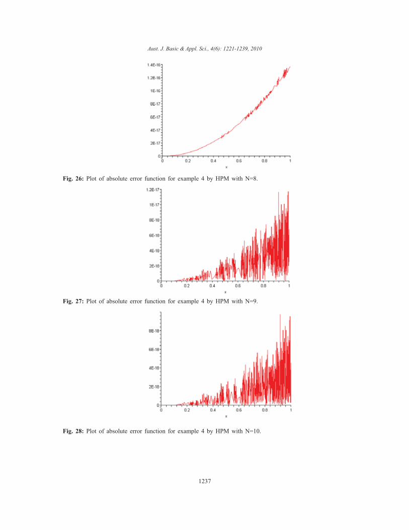
Fig. 26: Plot of absolute error function for example 4 by HPM with N=8.
Fig. 27: Plot of absolute error function for example 4 by HPM with N=9.
Fig. 28: Plot of absolute error function for example 4 by HPM with N=10.
1237
Aust. J. Basic & Appl. Sci., 4(6): 1221-1239, 2010
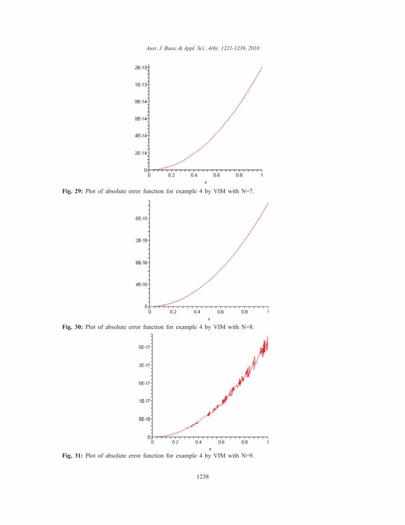
Fig. 29: Plot of absolute error function for example 4 by VIM with N=7.
Fig. 30: Plot of absolute error function for example 4 by VIM with N=8.
Fig. 31: Plot of absolute error function for example 4 by VIM with N=9.
1238
Aust. J. Basic & Appl. Sci., 4(6): 1221-1239, 2010
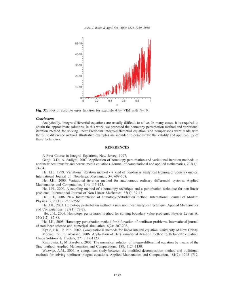
Fig. 32: Plot of absolute error function for example 4 by VIM with N=10.
Conclusion:Analytically, integro-differential equations are usually difficult to solve. In many cases, it is required to
obtain the approximate solutions. In this work, we proposed the homotopy perturbation method and variationaliteration method for solving linear Fredholm integro-differential equation, and comparisons were made withthe finite difference method. Illustrative examples are included to demonstrate the validity and applicability ofthese techniques.
REFERENCES
A First Course in Integral Equations, New Jersey, 1997.Ganji, D.D., A. Sadighi, 2007. Application of homotopy-perturbation and variational iteration methods to
nonlinear heat transfer and porous media equations. Journal of computational and applied mathematics, 207(1): 24-34.
He, J.H., 1999. Variational iteration method - a kind of non-linear analytical technique: Some examples.International Journal of Non-linear Mechanics, 34: 699-708.
He, J.H., 2000. Variational iteration method for autonomous ordinary differential systems. AppliedMathematics and Computation, 114: 115-123.
He, J.H., 2000. A coupling method of a homotopy technique and a perturbation technique for non-linearproblems. International Journal of Non-Linear Mechanics, 35(1): 37-43.
He, J.H., 2006. New Interpretation of homotopy-perturbation method. International Journal of ModernPhysics B, 20(18): 2561-2568.
He, J.H., 2003. Homotopy perturbation method: a new nonlinear analytical technique. Applied Mathematicsand Computations, 135(1): 73-79.
He, J.H., 2006. Homotopy perturbation method for solving boundary value problems. Physics Letters A,350(1-2): 87-88.
He, J.H., 2005. Homotopy perturbation method for bifurcation of nonlinear problems. International journalof nonlinear science and numerical simulation, 6(2): 207-208.
Kythe, P.K., P. Puri, 2002. Computational methods for linear integral equation, University of New Orlans.Momani, Sh., S. Abuasad, 2006. Application of He’s variational iteration method to Helmholtz equation.
Chaos Solitons & Fractals, 27: 1119-1123. Rashidinia, J., M. Zarebnia, 2007. The numerical solution of integro-differential equation by means of the
Sinc method, Applied Mathematics and Computations, 188: 1124-1130.Wazwaz, A.M., 2006. A comparison study between the modified decomposition method and traditional
methods for solving nonlinear integral equations, Applied Mathematics and Computation, 181(2): 1703-1712.
1239