the use of wavelet transforms for x-ray diffraction … use of wavelet transforms for x-ray...

$: The Use of Wavelet Transforms for X-ray Diffraction … USE OF WAVELET TRANSFORMS FOR X-RAY DIFFRACTION ANALYSIS Simon Bates: Krutos Analytical Inc., 100 Red Schoolhouse Rd., Chestnut$
THE USE OF WAVELET TRANSFORMS FOR X-RAY DIFFRACTION ANALYSIS

Simon Bates: Krutos Analytical Inc., 100 Red Schoolhouse Rd., Chestnut Ridge, NY 10977

Abstract In this paper, the applicability of wavelet methods to the analysis of x-ray diffkaction data will be generally discussed. Wavelet methods are similar to Fourier methods in their wide ranging applicability to x-ray diffraction but whereas the Fourier approach is based upon continuous sine and cosine functions, the wavelet approach is based upon functions that are localized in space and time. This makes them suitable for the analysis of discreet events and localized phenomena. The development of a Wavelet Transform method will be discussed and directly applied to the identification of unknown polycrystalline phases.

Introduction Wavelet methods, like Fourier methods, can be applied to the analysis of x-ray diffraction data from two different perspectives. The first of these is the development of fundamental methods, which can be used to simulate diffraction processes and then model the measured data based upon a description of the sample. The second approach is to apply wavelet transforms directly to the measured data in order to mathematically extract useful information. In the first approach, wavelet methods promise to lead to new insights into the processes of diffraction using an ‘atomisitic’ approach to the solution of the diffracted wave equations. The wavelets used to describe the incident and diffracted wave vectors are highly localized and defined in terms of scale and time hence the label atomistic. In contrast, the more usual Fourier approach defines the wave-vectors in terms of their frequency or wavelength and treats them as a continuous electromagnetic wave. The atom&tic approach can be used to model distortions in the wave-vectors caused by the difEaction process and introduces concepts such as localized correlation lengths of interaction. The wavelet methods required to simulate diffraction processes have not as yet been completely defined. In this paper the focus will be on wavelet transform methods used to analyze measured data. The wavelet transform reduces the measured data set to a small number of wavelet coefficients. This reduced set of coefficients can be directly manipulated mathematically.

Development of Wavelet methods In Fourier space, the basis functions used to describe the analyzed data set are sine and cosine functions. After the application of the Fourier transform the analyzed data set is broken down into a set of sine and cosine functions of differing frequencies. The amplitude of these sine and cosine functions make up the Fourier coefficients of the data. In wavelet space, there are an infinite number of basis functions that can be used for a wavelet transform. However, each of these basis functions must be localized and consist of a damped oscillation centered on zero. So something like a typical Gaussian function cannot be used as a wavelet basis function. The wavelet basis functions are described in terms of scale and time. That is the oscillation exists over a certain distance and for a

Copyright(C)JCPDS-International Centre for Diffraction Data 2000, Advances in X-ray Analysis, Vol.42 251Copyright(C)JCPDS-International Centre for Diffraction Data 2000, Advances in X-ray Analysis, Vol.42 251ISSN 1097-0002

http://www.icdd.com

This document was presented at the Denver X-ray Conference (DXC) on Applications of X-ray Analysis. Sponsored by the International Centre for Diffraction Data (ICDD). This document is provided by ICDD in cooperation with the authors and presenters of the DXC for the express purpose of educating the scientific community. All copyrights for the document are retained by ICDD. Usage is restricted for the purposes of education and scientific research. DXC Website – www.dxcicdd.com

ICDD Website - www.icdd.com

ISSN 1097-0002

http://www.dxcicdd.com/

http://www.icdd.com/

certain time with differing degrees of localization and smoothness. The basis function can be used to describe complex data sets by translation and scaling. Following the development of Kaiser [ 11, if the wavelet basis function is taken to be w(u) then the scaled and translated version becomes: w&u) = ]s]‘pv((u-t)/s) ( where s is the scaling, t is the translation and p is arbitrary} To illustrate a basis function, a simple example is v(u) = u exp(-u2). This function is shown in the following diagram.

Wavelet Basis Function

OS I

-40 -20 0 20 40 U

In Fourier analysis, the advent of the Fast Fourier Transform method greatly speeded up the mathematical application of Fourier analysis and made the use of Fourier analysis realistic for general application, A similar Transform also exists for wavelet analysis. The application of this ‘black box’ Wavelet Transform allows a rapid breakdown of a complete data vector into its wavelet components. The following method development is presented in great detail with computer code in the Numerical Recipes [2] To apply the Wavelet Transform, the wavelet basis function is described by a series of wuveletfilter coeflcients. The most common set of wavelet basis functions expressible by filter coefficients were discovered by Daubechies [3]. The simplest and most localized member of this wavelet family called the DAUB4 has only four coefficients CO,C~,C~,C~. The application of the filter coefficients to the data vector can be expressed in a matrix format :

1 co cl c2 c3 I 1 c3 -c2 cl -co I

co cl c2 c3 c3 -c2 cl -co I

1. ’ I

1: : . I co cl c2 c3 1 c3 -c2 cl -co 1

1 c2 c3 co cl I 1 cl -co c3 -c2 1


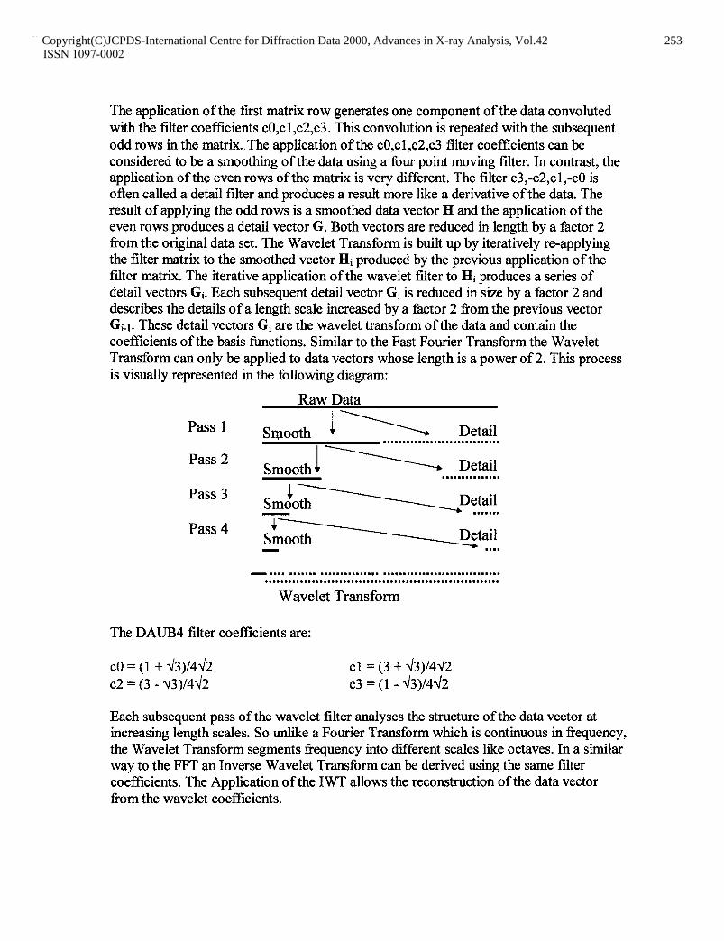
The application of the first matrix row generates one component of the data convoluted with the filter coefficients cO,cl ,c2,c3. This convolution is repeated with the subsequent odd rows in the matrix., The application of the cO,c 1 ,c2,c3 filter coefficients can be considered to be a smoothing of the data using a four point moving filter. In contrast, the application of the even rows of the matrix is very different. The filter c3,-c2,cl,-CO is often called a detail filter and produces a result more like a derivative of the data. The result of applying the odd rows is a smoothed data vector H and the application of the even rows produces a detail vector G. Both vectors are reduced in length by a factor 2 from the original data set. The Wavelet Transform is built up by iteratively re-applying the filter matrix to the smoothed vector Hi produced by the previous application of the filter matrix. The iterative application of the wavelet filter to Hi produces a series of detail vectors Gi. Each subsequent detail vector Gi is reduced in size by a factor 2 and describes the details of a length scale increased by a factor 2 Tom the previous vector Gi-1. These detail vectors Gi are the wavelet transform of the data and contain the coefficients of the basis functions. Similar to the Fast Fourier Transform the Wavelet Transform can only be applied to data vectors whose length is a power of 2. This process is visually represented in the following diagram:

Pass 1

Pass 2

Raw Data

Smooth 1 \ Detail . . . . . . . . . . . . . . . . . . . . . . . . . . . . . .

Smooti/ L D&l l . . . . . . . . . . . . . .

-. ... ....... ............... .............................. ............................................................

Wavelet Transform

The DAUB4 filter coefficients are:

CO = (1 + 43)/442 cl = (3 + 43)/442 c2 = (3 - 2/3)/442 c3 = (1 - 1/3)/442

Each subsequent pass of the wavelet filter analyses the structure of the data vector at increasing length scales. So unlike a Fourier Transform which is continuous in frequency, the Wavelet Transform segments frequency into different scales like octaves. In a similar way to the FFT an Inverse Wavelet Transform can be derived using the same filter coefficients. The Application of the IWT allows the reconstruction of the data vector from the wavelet coefficients.


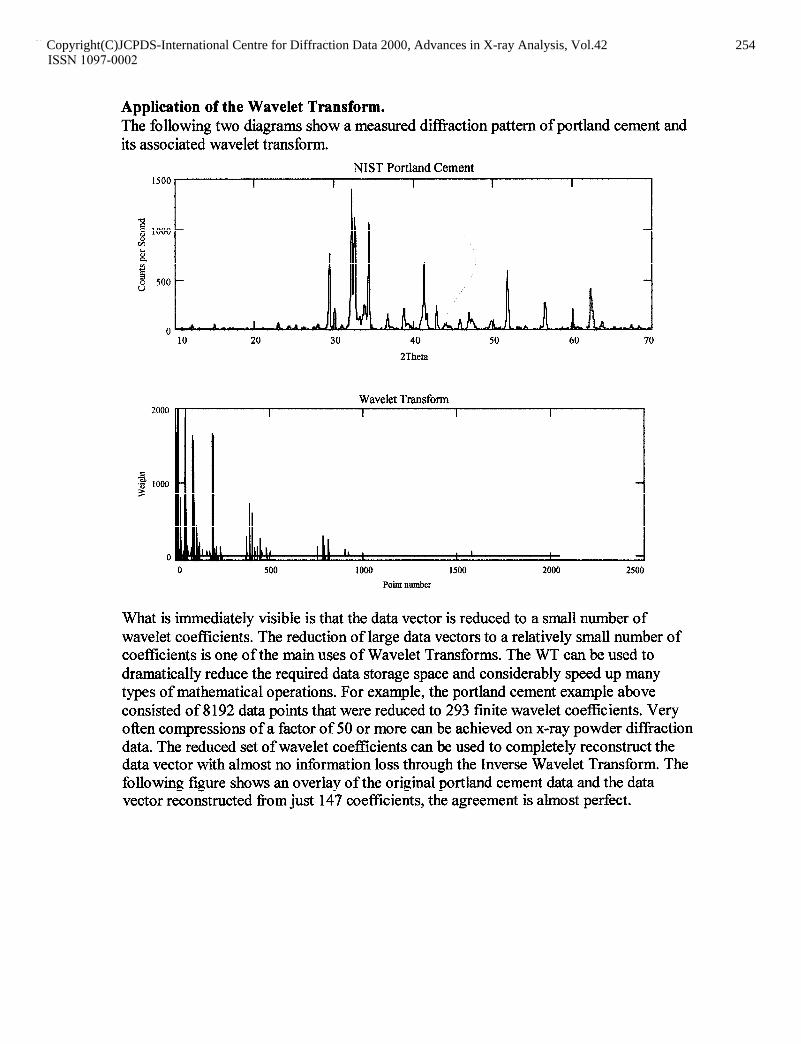
Application of the Wavelet Transform. The following two diagrams show a measured diflkaction pattern of portland cement and its associated wavelet transform.

I NIST Portland Cement

I I I I

I

40 50 60 70

2Theta

Wavelet Transform

0 500 1000 1500 2000 2500

Point number

What is immediately visible is that the data vector is reduced to a small number of wavelet coefficients. The reduction of large data vectors to a relatively small number of coefficients is one of the main uses of Wavelet Transforms. The WT can be used to dramatically reduce the required data storage space and considerably speed up many types of mathematical operations. For example, the portland cement example above consisted of 8192 data points that were reduced to 293 finite wavelet coefficients. Very often compressions of a factor of 50 or more can be achieved on x-ray powder diffraction data. The reduced set of wavelet coefficients can be used to completely reconstruct the data vector with almost no information loss through the Inverse Wavelet Transform. The following figure shows an overlay of the original Portland cement data and the data vector reconstructed Corn just 147 coefficients, the agreement is almost perfect.


NIST Portland Cement 600 I I I

“2 2 400 - d

k

8 s 200 - h -

. 0- .AlL.d L Ifh¶

20 25 30 35 40

2Theta

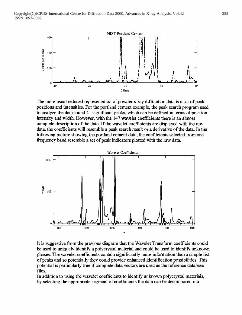
The more usual reduced representation of powder x-ray diffraction data is a set of peak positions and intensities. For the Portland cement example, the peak search program used to analyze the data found 41 significant peaks, which can be defined in terms of position, intensity and width. However, with the 147 wavelet coefficients there is an almost complete description of the data. If the wavelet coefficients are displayed with the raw data, the coefficients will resemble a peak search result or a derivative of the data. In the following picture showing the portland cement data, the coefficients selected from one frequency band resemble a set of peak indicators plotted with the raw data.

Wavelet Coefficients

0

800 1200 1400 1600 1800

”

It is suggestive from the previous diagram that the Wavelet Transform coefficients could be used to uniquely identify a polycrystal material and could be used to identify unknown phases. The wavelet coefficients contain significantly more information than a simple list of peaks and so potentially they could provide enhanced identification possibilities. This potential is particularly true if complete data vectors are used as the reference database files. In addition to using the wavelet coefficients to identify unknown polycrystal materials, by selecting the appropriate segment of coefficients the data can be decomposed into


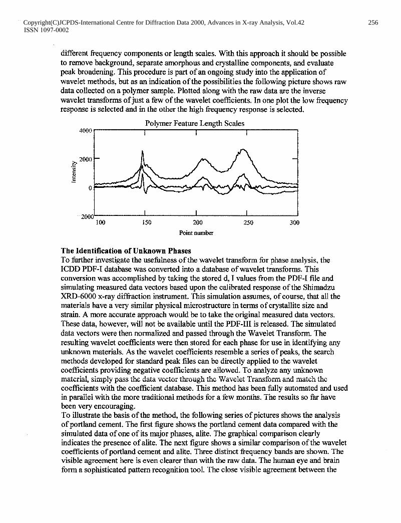
different frequency components or length scales. With this approach it should be possible to remove background, separate amorphous and crystalline components, and evaluate peak broadening. This procedure is part of an ongoing study into the application of wavelet methods, but as an indication of the possibilities the following picture shows raw data collected on a polymer sample. Plotted along with the raw data are the inverse wavelet transforms of just a few of the wavelet coefficients. In one plot the low frequency response is selected and in the other the high frequency response is selected.

Polymer Feature Length Scales

4ooo I

I 200

Point number

I I 250 300

The Identification of Unknown Phases To further investigate the usefulness of the wavelet transform for phase analysis, the ICDD PDF-I database was converted into a database of wavelet transforms. This conversion was accomplished by taking the stored d, I values from the PDF-I file and simulating measured data vectors based upon the calibrated response of the Shimadzu XRD-6000 x-ray diffraction instrument. This simulation assumes, of course, that all the materials have a very similar physical microstructure in terms of crystallite size and strain. A more accurate approach would be to take the original measured data vectors. These data, however, will not be available until the PDF-III is released. The simulated data vectors were then normalized and passed through the Wavelet Transform. The resulting wavelet coefficients were then stored for each phase for use in identifying any unknown materials. As the wavelet coefftcients resemble a series of peaks, the search methods developed for standard peak files can be directly applied to the wavelet coefficients providing negative coefficients are allowed. To analyze any unknown material, simply pass the data vector through the Wavelet Transform and match the coefficients with the coefficient database. This method has been fully automated and used in parallel with the more traditional methods for a few months. The results so far have been very encouraging. To illustrate the basis of the method, the following series of pictures shows the analysis of Portland cement. The first figure shows the Portland cement data compared with the simulated data of one of its major phases, alite. The graphical comparison clearly indicates the presence of alite. The next figure shows a similar comparison of the wavelet coefficients of portland cement and alite. Three distinct frequency bands are shown. The visible agreement here is even clearer than with the raw data. The human eye and brain form a sophisticated pattern recognition tool. The close visible agreement between the


two sets of wavelet coefficients clearly indicates the power of this approach. As more data is accumulated, a statistical analysis will be performed comparing the results of the

NIST Portland Cement + Alite I I I I I

1000 -

% 3 s D

i Ii

8 ii

30 32 34 36 38 40 42 44

2Theta

wavelet search methods with the results of the more traditional approaches.

WT of Portland cement 62 Alite

150

Point number

200 250

References [l] Gerald Kaiser, 1994, A Friendly Guide to Wavelets, (Birkhauser) [2] W.H. Press et al, 1992, Numerical Recipes in C, 2nd edition, pp. 591-606 (Cambridge University Press) [3] I. Daubechies, 1988, Communications on Pure and Applied Mathematics, vol. 41, pp. 909-996


the use of wavelet transforms for x-ray diffraction … use of wavelet transforms for x-ray...

Documents