the use of wetland bird species as indicators of land
TRANSCRIPT

•
The Use of Wetland Bird Species as Indicators
of Land Cover Change within the Mgeni
Estuary and Beachwood Mangrove Swamps
Andrew Paul Batho
Submitted in Fulfilment of the Requirements for the
Degree of Master of Social Science (Masters by Research in Geography and Environmental Science)
School of Environmental Sciences
Faculty of Humanities, Development and Social Sciences
University of KwaZulu- Natal
May 2010

DECLARATION
Submitted in fulfilment / partial fulfilment of the requirements for the degree
of ... ... ...... ......... ...... ..... , in the Graduate Programme in
.............................. , University of KwaZulu-Natal,
South Africa.
I declare that this dissertation is my own unaided work. All citations,
references and borrowed ideas have been duly acknowledged. I confirm that
an external editor was / was not used (delete whichever is applicable) and
that my Supervisor was informed of the identity and details of my editor. It
is being submitted for the degree of ................................................. in
the Faculty of Humanities, Development and Social Science, University of
KwaZulu-Natal, South Africa. None of the present work has been submitted
previously for any degree or examination in any other University.
Student name
Editor

Abstract
Because of the variety of ecological and economic functions they perform, estuaries and
mangrove swamps are recognised as amongst the most valuable habitats on earth.
However, estuaries and related mangrove swamps are threatened by human expansion and
exploitation which leads to changes in land cover change within and surrounding these
sensitive ecosystems. Such land cover changes can either have desirable or undesirable
effects on natural ecosystems. Examples of undesirable impacts of land cover change
include soil erosion and degradation, the removal of indigenous vegetation for human
development, and the pollution of water. Without an effective means of identifying,
monitoring and managing land cover changes over time, these sensitive ecosystems face a
bleak and uncertain future.
The researcher sought to determine whether wetland bird species could be used as an
effective method of monitoring the environmental health of estuaries and mangrove swamps.
In particular, the research sought to determine whether analysing fluctuations in the
populations of wetland bird indicator species, as evident in the CWAC Bird Census data,
could assist in monitoring and assessing undesirable and desirable land cover changes
within the Mgeni Estuary and Beachwood Mangrove Swamps.
An examination of the archival aerial imagery of the study area for the years 1991, 1997,
2003 and 2008 provided by the University and private companies, revealed significant
changes in land cover over the last two decades. The land cover changes identified
represent an actual decline or increase in the suitable foraging, roosting or reproductive
habitats of wetland bird indicator species within the study area. The research focused on
investigating whether fluctuations in wetland bird populations can be correlated with the
recorded changes in land cover over the last two decades. The research discovered a direct
and comprehensive link between fluctuations in specific populations of wetland bird indicator
species and the land cover changes identified within the study area over a 20 year period.
ii

Declaration
The work described in this dissertation was carried out in the School of Environmental
Sciences, University of KwaZulu Natal, from March 2008 to October 2009. This work was
undertaken under the supervision of Prof. F. Ahmed
This study represents the original work of the author and has not otherwise been submitted
in any form, in part or in whole, for any degree or diploma to any other university. Where use
has been made of work by others, this has been duly acknowledged in the text.
Signed __ --'-pg;t~~--------
A.P.Batho ·
Supervisor:
Prof. F. Ahmed
Signed ------,.4f-f.+f-.-'-----
iii
Acknowledgements
There are many people without whose help this study would not have been possible and to
whom I am indebted for their guidance and assistance:
• Dr. F. Ahmed (School of Environmental Sciences) for his supervision of this study, and
his encouragement, advice and assistance in compiling this work.
• Dr H. Watson (School of Environmental Sciences) for initiating the study.
• Ms C. Reid (School of Environmental Sciences) for her assistance and guidance in using
GIS correctly.
• Mr E. Powys (School of Environmental Sciences) for allowing access to the School of
Environmental Sciences Library and the aerial imagery.
• Mr D. Allen (Natural History Museum) for his assistance and advice in regard to wetland
bird species during this study.
• Mr R. Cowgill and Mr S. Davis (Birdlife International) for their guidance and assistance in
the selection of the research topic and for allowing the researcher to use their library.
• Mr M Webber (Avian Demographic Unit, University of Cape Town) for providing the
researcher with all CWAC Avian Census Data at his disposal.
• Mr J Gillard (Honorary Ezemvelo KZN Wildlife Official) for assisting with field surveys
and giving the researcher access to the Beachwood Mangrove Reserve.
• Mr B. Land (Map Centre CC) for his assistance with the aerial imagery.
• A special thanks to Mr R. Botes for taking time out of his busy schedule to assist the researcher with reviewing and editing this thesis.
• Prof A. Dales, Prof M. Mathews and Mr C. Venter for their assistance with the statistics.
• Finally, thanks to my friends Charlene, Colleen and Petar for all their support and
assistance gathering field data.
• To my family for all their love, support and encouragement over the last two years.
iv

Table of Contents
Abstract ... .. .. ......... .... ............ .. ... ............... ..... ... ........ ..... ...... .. .... ... ................ .. ... ..... .. ............ ii
Declaration .. .. ... .... .... ........ ... .......... ................... .... .. .... .......... ..... .. .. ...... ............... .. .. .... .. .. ..... iii
Acknowledgements .. .. .......... .......... .... ... .. .. ... ... .. ... ... ... ......... .. ..... .. ... .......... .. .... .. ... ...... ...... .. iv
Table of Contents ...... ........... .. .... .. .... ... .......... .. ..................... .. ..... ........ ...... ..... ... .... .. : ...... .... .... v
List of Plates ..... ........ .. .... .... .. ... ..... ... ...... .. .... ... .. ... ..... ... ......... .......... ... ....... .. ... ... ......... ... ....... ... x
List of Figures ........... ..... .. ... ................. ... .... ..... ........ .... ... .. ... ........... ........ .... ...... ... .. .... ......... . xiii
List of Tables ... ......... ........ .. ...... ........... .... ... ... ......... .. ..... ....... ................. ........ .. ..... ............ .. xviii
Chapter One: Introduction ................................................................................ ............ . 1
1.1 Background and Outline of Research ...... .. ...... ........ ...................... .. .......... ..... ................. 1
1.2 Land Cbver Change .. .. ............ .. ..... ....... .................. .... ... .......... .... ....... ...... .. ..... .... ....... ... 2
1.3. Land Use Change ... ........ .. .. ... ..... ........ .. .. ................ ............ ......... ... ............................... 3
1.4. The Significance of the Study .. ........ ... ..................... .............. ...... ........................ ........... 3
1.5. The Importance of the Mgeni Estuary and Beachwood Mangrove Swamps ................... 4
1.6. Aim of Study .......... .......... ..... ............ ............................................................................. 5
1.7. Objectives of Study .... ... .. ... .... .. ..... ... .... ....... ..... .. ...... .... .. .... ... .... .......... ..... ..... .... .... .. ....... 5
1.8. Structure of Thesis .... ........ .............. .. ....................... ..... .. .. ... ........ ... ...... .. .. ........ ......... .... 6
Chapter Two: Literature Review ...... ................................. .. ....... .. .. ........... ......... ............ 7
2.1. Introduction .............. .. ..... .......... ... .......................... ... .......... .. ... ... .............. ... .......... ... ..... 7
2.2. South African Estuaries and Mangrove Swamps ............................................................ 7
2.3. Tidal Influence on Estuarine and Mangrove Ecosystems .... ...... .... .......... .... ... .. .... .. .. .... .. 8
2.4. The Ecological and Economic Benefits of Estuaries and Mangrove Swamps ................. 9
2.5. Birds within Estuarine and Mangrove Ecosystems ................. ...... .... ............ .. .... .. .. .. .... 14
2.6. Diet and Foraging Behaviour of Estuarine Bird Species .......... ........... .. .. .. .... .. ....... ...... . 16
v
2.7. Birds as Indicators of Environmental Change ...... ... ..... ....... .... ...... ... .. ... ..... ... .. ..... ......... 20
2.8. Avian Census Data and its Contribution to Environmental Monitoring ....... .. ........ ... ..... . 23
2.9. Using Birds as Environmental Indicators in Estuaries .......... ......... .... ......... .. ...... .. ..... ... 25
2.10. Assessment of Land Cover Changes ...... ... .... ... .. ......... .. ..... .... .. ....... ... .... ........... ........ 28
2.11. Summary ... .. .... ...... .... ... ........ ...... ... ..................... ........ .. .... ..... .. ....... .. ......................... 30
Chapter Three: Background to Study Area .......... ...... .. ........ .. ........ ................. .. ........ 32
3.1. Introduction ........... ... ...... ....... ................. ... ............ .. ... .... .............. ..... .... ... .. .... ........ .. .. .. 32
3.2.Background ...... ..... .... ... .. ........................ ........... .... ... ...... .... ..... ..... .... .... ...... ... ................ 32
3.3.Mgeni Catchment and Estuary ... .. ....... ..... ... ....... .. ......... ........... ............ .. ......... .. ... ...... ... 33
3.4. Climate ................ ......... .... ........ .... ........ ............... .............................................. ... ....... 36
3.5. Soil and Topology .... .... .. .. .............. ........ ............ .. .... .. .. .... .. .. ........ .................... .... ........ 37
3.6. Sediment ............. .... ...... .. ............ .. .... ........ ..................... .. .. ... ................. ..................... 38
3.7. Area and Extent of the Estuary and Mangroves ........ .. .................................. ..... .. ........ 38
3.8. Current Health of Mgeni River and Estuary .. ................................................................ 39
Chapter Four: Materials and Methods .. .. .. ..... .. ................................... ...... .. .. ...... ....... 41
4.1. Introduction .................. ............................ ...... .......... .... .. ........................ .... .................. 41
4.2. Materials Used in the Study ...... .. .............................. ...... ...... .. .. .. ... .............................. 41
4.2.1. Data on Wetland Bird Species ...... .. ...... ............ ........... ............................ .......... 41
4.2.1.1 The Total CWAC Repoli-Coordinated Waterbird Counts in South Africa .. ......... 41
4.2.1.2. Interviews with Local Ornithological Experts ...... .... ......................... ... ........ ........ .. 42
4.2.1.3. Archival Aerial Imagery .................. .. ....................................................................... 42
4.2.1.4. Discounted Material ....... ................. .. ...................... .. ................... .. ... ...................... 43
4.3. Methods Used in the Study .... ................... .............. ..... ............................. ... ........ ... ... .. 44
4.3.1 . Evaluating Land Covel' Change ......... ..... .. .. ..... .. .............. .... ..................... ..... .... 44
4.3.1.1. Land Cover Classification System ................ ...... .... ... .. .......... ... ............................. 44
vi

4.3.1.2. The Impacts of Tidal Fluctuations on Study Area ... .............. .... .. .................. ... 47
4.3.1.3. Scanning of Aerial Imagery .. ..... .......... .. ... ... .. ...... .. .... ..... .. .... ..... ..... ... .. ... ... ... ... 49
4.3.1.4. Georeferencing ... .................. .. ..... ... ..... ....... ... ........ .. .... ... .. ..... ...... .. .... ... ................... 50
4.3.1.5. On-Screen Digitizing ............................................ ...... .. ......... ............. ....... ............. . 50
4.3.1.6. Projecting Land Cover Maps ....... .... ........ .... .. ............. ... ... .. ... ....... ... ... ... ... ........ .. ... . 51
4.3.1.7. Assessing Changes in Land Cover .................... ...... .. ...... .. .................. ..... .. .... ... ... 52
4. 3.1.8. Positional Error ................ .. ..... .. ....................................... .. ........ .. .... ..................... .. 52
4.4. Identification of Avian Indicators ....... .. ......... ... ..... .. .. .......... .. .... ....... ....... ........... .... ... ..... 53
4.4.2. Identification of Indicator Species ... ...... ..... ..... ....... .... ..... ...... .. .... ........ ... .. ... ... .. .. . 53
4.4.3. Criteria Utilised for Selecting Avian Indicators .. ..... .... .. ... .... ... ........... .. ... ... .. .. ...... 54
4.4.4. Analyzing the CWAC Bird Census Data ..... ...... ............. ... .... ... ........ ..... ... .. ......... 55
4.4.5. Interviews with Local Ornithologists ....................... ...................... ... ... ... ......... .... 56
4.4.6. Field Survey of current status of Mgeni Estuary and Beachwood Mangrove
Swamps ...... .. .. .............. .... ... .. ... .. .. .... .. ... .... .. ... ..... .. ..... ... ... ... .. ........... ... .. .... ..... ... .......... 57
4.5. Assessing the Relationship between Counts of Wetland Bird Indicators and Changes in
Land Cover ......... .... ... ........ .. ....... ...... ..... .... ................. ....... ... .......................... ... ............... .. 58
4.5.1. Statistical Analysis and the Correlation Coefficient... ........ ................ ......... ... ...... 58
Chapter Five: Results and Discussion ................................................. .. .. .... .. ........ ... 65
5.1. Categorization and Mapping of Changes in Land Cover within the Study Area ..... 65
5.2. Land Cover Change within the Study Area ..... ...... .............................. .... .. ...... .. ............ 65
5.4. Open and Shallow Water Bodies Land Cover Sub-Classes ........ .......... ...... ... .... .. ........ 68
5.5. Corrected Exposed Mudflat Land Cover Class ............. .. ... ...... ..... ... ...... ..... .. .. ... .. .. .... ... 71
5.6. Wooded Land Cover Classes ...................................................... .. ............................... 72
5.7. Grassland, Scrubland and Reed Bed ... ....... ........ ....... ........... ... ........ .............. ... ........... 79
5.8. Other Vegetation Land Cover .. .... .. ... ...... ........... .. ............. .. .. ... .......... ........ ... ... ... .... ... .. . 82
5.9. Other Land Cover Classes ............................................... ...... ....... ...... .. .......... .. ........... 87
5.10. Land Cover Change within the Study Area ........ .. ..... ............ ....... ... .............. ........... ... 91
vii

5.11 . Changes in Avian Indicator Populations within the Mgeni Estuary and Beachwood Mangrove Swamp Ecosystem. .... ... .... .. ... .. .... ... ....... .... ..... .. ... ......... .. .. ...... .. ... .... ....... ... .... . ... 92
5.12. Open Water Avian rndicator Species .. ... ............. ... ....... ..... ... .. ... .. .............. ...... ... . 92
5.13. Shallow Water Avian Indicator Species .... .... ... ....... .. .............. ...... .... ..... ..... ..... .... ....... 99
5.14. Mudflat Avian Indicator Species ........ .. .... ........................ .... ......................... .... ........ 105
5.15. Vegetated Area Avain Indicator Species ........ ......... .. ........ .. ........ .... ............ .. .. ......... 113
5. 16. Beach and Sand Bank A vian Indicator Species ... ........ .. ... .................... .. .... .. .. ........ .. 119
5.17. Relationship between Changes in Land Cover and Avian Indicator Numbers .......... 126
5.18. Stabilisation of Vegetated Islands and Shoreline Vegetation, and the Increase in Vegetable Areas and Shoreline Zone Indicator Bird Species ........... .. ................... ........ .. .. 126
5.19. Decline in Grassland and Scrub Land Cover Crass ...................... .. ...... .. ................ .. 132
5.20. Expansion of Island Mangrove Land Cover Class and Impact of Vegetated Avian Indicator Populations ....... ..... ..... ..... .... ....... .... .... ........... .... ... ... .. .. ............ ........ ..... ... .. ..... ... 136
5.21. Reduction in Sediment, and the Subsequent Impact on Mudflat, Dune and Shoreline Avian Indicators ........................... ........ ... .. ....................... .. ........ ...... .. ....... ......... ....... ........ 140
5.22. Mangrove Vegetation Expansion and the Decline of Mudflat Habitats and Avian
Indicators .. ..... ...... ... ... ... ..... ........ .. .. ... .............. ..... ...... .............................. .. ... ........... ......... 147
5.23. Water Land Cover Classes within the Mgeni Estuary and Beachwood Mangrove Swamps ........ .. .... ..... .............. ..... .......... ............. .... .... ........ ..... ...... ...... .... .... .. ........... ... ..... . 159
Chapter Six: Conclusion and Recommendations ........ ... .............. ........................ 167
6.1. Inconsistencies in the Avian Census Data Set Acknowledged ... .. ...... ............. ...... ..... 167
6.2. General Conclusion .......... .. .................................................... ........... ........................ 169
6.3. Future Applications of this Study ............ ...... ..... .......... ...... .... ..... ......... ..... .............. .... 172
6.4: Recommendations .. ..................... ....... .............................. .. .. ........................................ ..... .... .. ... 173
References ... .... ......... .. ... .... ................ ......... ................... ........... ... .......... .... ....... .. ...... ... ... .. .... .......... 175
Appendix ...... .... .. ... ..... ... ...................... ....... ... ...... ......... ........... .. ........ .. ...... ...... ..... ... ........ 181
Appendix A: Land Cover Type Figures .... .... .... ... ......... .......... ............ .... ... .......... .... ... 181
viii

Appendix B: Comparison between Avian Indicator Populations (1993-2008) ............. 186
Appendix C: Wetland Avian Indicator Species .... ........ .. ............ .................... ............ 190
Appendix D: Orientation Map .. ............... ........ ... .. .... .. .... ....... ... ........................ ........... 194
Appendix E: Estuarine and Mangrove Avian Indicator Species Provide by David Allen ............................................................................................................. ...... .. ............. 195
Appendix F: Ornithologist Report on Avian Indicator Species .................................... 212
Appendix G: Land Cover Classes .............................................................................. 216
Appendix H: CWAC Data Permisson Request Form ....... ............. ............... ........ ...... . 218
Appendix I: Review of Avian Indictor Performance as Land Cover.Change Indicator Species ................. .. ............ .................... .... .. ........ ... .... .... ....... ... ..... ........................... ...... 220
Appendix J: Criteria Utilised for Selecting Avian Indicators .. .. .... .... ......................... .. ...... 222
Appendix K: Aerial Imagery (1991-2008) ............................................ ............ ...... ........... 225
ix

List of Plates
Plate 1: The Study Area in Relation to KwaZulu-Natal. ...... .... ..... .. .. ... .......... ... .... ....... ... ....... 32
Plate 2: Mgeni Estuary Mouth ... .... .. ............................. .. ... ....... ..... ... ...... ..... ........... ........ .... .. . 33
Plate 3: River through Beachwood Mangrove Swamps .................... ... ... .. .. ........ ... ... ... ..... .... 34
Plate 4: Map of Mgeni Estuary and Beachwood Mangrove Swamps .................................. .. 36
Plate 5: Beachwood Mangrove Swamps .............. ... ....... ... .... .. .... ........... ..... ...... .... ... .. ...... ..... 39
Plate 6: Island and Vegetation ...... .. .. .. ........ ............. ... .............. .......... .. ....................... ..... .... . 63
Plate 7: Mgeni Estuary and Beachwood Mangrove Swamps 1991 Land Cover .. ................ . 61
Plate 8: Mgeni Estuary and Beachwood Mangrove Swamps 1997 Land Cover .... .. .... .. .. .. .... 62
Plate 9: Mgeni Estuary and Beachwood Mangrove Swamps 2003 Land Cover .................. 63
Plate 10: Mgeni Estuary and Beachwood Mangrove Swamps 2008 Land Cover .. ... .. ...... .... 64
Plate 11: Open Water .................. .. ........................................................... .. .. .... .. .................. 68
Plate 12: Open Water ...... .... ......... .. ....................... ...... .................. .. .. ..... ..... .. ...... ....... ........ .. 69
Plate 13: Shallow Water. ... ................. .. ... .................... .......... .... ....... ..... ...... ... ...... ........... ..... 71
Plate 14: Woodland, Grassland and Scrub Land Cover Classes ........ ...... ........... .. .......... .... . 74
Plate 15: Mangrove Vegetation ..... .............. ... .... .............. ........ .. .......... ......... ........ .. ...... ........ 77
Plate 16: Woodland and Mudflat Land Cover ............ .. .... .. ....................... .......... .. ..... ........ .... 78
Plate 17: Island Mangrove Vegetation ....... ................................ .... .. ... .. .. ...... ........ ..... ..... .. .. ... 78
Plate 18: Reed Beds and Marsh ................ .... .... .............. .. .. .. ...... ...... .. .... .. .. .. ...... .. .. .. .......... .. 80
Plate 19: Reed Beds and Grassland .... .... .... ...... ............ .. .. .. ..... .. .. ....... .. .. .... ........... ........ .... .. 82
Plate 20: Salt Marsh .. ............. .. ...... .... ..... .... ... ......... .......................... .. ....... ..... .. ................... . 82
Plate 21: Transission from Salt Marsh to Mangrove Vegetation .. ..... ..... .. ... ... ...... ........... ..... .. 85
Plate 22: Dune Vegetation and Beach ..... ...... ....... .... ..... ..... ....... ......... ... .. .... .. ...... .. .... ............ 85
x

Plate 23: Sand Banks at Estuary Mouth ... ... ....... .. ......... ................ .. ....... ........................... .... 86
Plate 24: Beach ....... ...... ..... .... ..... .. ..... .... .... ........ .. .. ....... ...... .. ...................... .. ...................... .. 87
Plate 25: Sand Banks .... ... ....... ........ .... ........ ........ ........ ........ ..... .. ... ......... ....... .......... .... .... ...... 88
Plate 26: Pink Pelican (Pelecanus rufescens) .... .. .................. ..... ..... ... ............ .. ... .. ... .... ... .. .. . 89
Plate 27: African Darter (Anhinga melanogaster) ......... ..... .... ..... ..... ..... ... ............ .. ... ............. 94
Plate 28: White Breasted Cormorant (Pha/acrocorax carbo) ................. .. ....... ........ .. ......... ... 98
Plate 29: Goliath Heron (Ardea goliath) .. ... ................. .. ...... .. ............. ........ ..... .. ............. ...... 1 00
Plate 30: Little Egret (Egretta garzetta) ............. .. .. ..... .... ..... ....... ..... ...... ...... ... ....... .............. 1 02
Plate 31: Pied Kingfisher (Geryle rudis) ................. ...... ... .......... .... ... .. .. ... .. ......... ....... ...... ..... 1 03
Plate 32: Little Stint (Galidris minuta) ........... ......... .... ............... ....... .......... ...... ....... .. ............ 107
Plate 33: Curlew Sandpiper (Galidris ferruginea) .... .. .. .. ......................... .. ... ......................... 108
Plate 34: Sacred Ibis (Threskiomis aethiopicus) ................ .. .......... ...... .. ...................... .. .... . 109
Plate 35: Black-Smith Plover (Vanelfus armatus) ................................ .... ............................ 113
Plate 36: Purple Heron (Ardea purpurea) ........ .................................................................... 115
Plate 37: Water Dikkop (Burhinus vericulatus) .............. .. .......................... .. ........................ . 117
Plate 38: Woolly-Necked Stork (Giconia episcopus) .. ................... .................... .... .............. 117
Plate 39: Caspian Tern (Hydroprogne caspia) ........................ .. .... .. ........ ............ ...... .......... 122
Plate 40: Grey Headed Gull (Larus cirrocephalus) .......... ...................... .. .... ............ ..... .. ..... 123
Plate 41: Swift Tern (Sterna bengil). .................. ... ...... ... ....... ....... .. .. ........... ...... .. ... ......... .... . 124
Plate 42: Mangrove Seedlings, Reeds and Grass Species on Island in the Mgeni
Estuary ............. .... .. .......... ...... .... .... .... .. ............ .. ... ... ... ... .... ................. .... ... ..... ... ... ............. .. 127
Plate 43: Reed Beds on Mgeni Estuary Island .............. ...... .......... .................. ...... ............... 130
Plate 44: Significant Land Cover Change witllin the Mgeni Estuary and Beachwood
Mangrove Swamps (1991-2008) .... ............................. ... .... ..... .. .. ............... .... .. ............... ... 141
Plate 45: Beach near Beachwood Mangrove Swamps .... .............. ...................... .. .. ........... 142
xi
Plate 47: Dense cluster of Avicennia Seedlings south of Athlone Bridge (Lower Esiuary) .. 150
Plate 48: Mangrove Seedlings Established on Mudflats near Mgeni Estuary Mouth ... .. ..... 151
Plate 46: Mgeni Estuary and Beachwood Mangrove Swamps Land Cover Changes (1991-
2008) .... ....... .... ...... .......... ... ....... ...... .... .. .... .... ..... ........ ... .. .... ...................... .. .. .... ....... .. .... ..... 152
Plate 49: Expansion of Mangrove Vegetation near Athlone Bridge (Connaught Bridge Side)
.... ... ... .... .. .... .. .... ... ... ..... ...... ....... .. .. .. ...... .. .... .... ..... ... ... ...... ... .... .. ...... .... ...... ....... .. .. .... .. .. ........ 153
Plate 50: Mangrove Vegetation Expansion- Former Mudflat Area .......... .. .. .. .. .. .... .. ........ .... . 156
Plate 51: Mangrove Tree Seed ... .. .. .. ....... .... .. ... ....... .. .... ....... ......................... .. ....... .... .. .... .. 157
Plate 52: Little Egret Hunting in Shallow Water Zone .... .............. .. .. ...... ... ...... .. ... .. .... ...... ... 161
Plate 53: Shallow Water in Mgeni Estuary ........ .. .... .. ...... .... ........................ .............. .. .. .. .. .. 166
xii

Table of Figures
Figure 1: Summary of the Steps Followed to Develop the Historical Land Cover Change
Database and Maps Vegetation within the Mgeni Estuary and Beachwood Mangrove
Swamps . ..... ...... ... ... .. ... .. .... .. . .. ........ .................. ... .. ..... ........ ........ ... .. .... .... ... .. .... 60
Figure 2: Decline in Area Coverage of Open Water Land Cover Class .... ......... .... ...... .... .... .. 69
Figure 3: Increase in Area Coverage of Shallow Water Land Cover Class .......... .... .. ..... ...... 70
Figure 4: Decline in Area Coverage of Exposed Mudflats Land Cover Class .......... ....... .. .... . 72
Figure 5: Increase in Area Coverage of Coastal Forest Land Cover Class ... ...... ..... ... ... .. ..... 74
Figure 6: Increase in Area Coverage of Woodland Land Cover Class ......... ........ ... ... ........ ... 75
Figure 7: Increase in Area Coverage of Mangrove ForestLand Cover Class ...... ... ...... .. .. .. ... 76
Figure 8: Increase in Area Coverage of Island Mangrove Land Cover Class .... ... .. ... ... ... .... . 76
Figure 9: Decline in Area Coverage of Grassland and Scrub Land Cover Class .. ... ....... ...... 81
Figure 10: Decline in Area Coverage of Reed Beds and Marshes Land Cover Classes .... ... 81
Figure 11 : Increase in Area Coverage of Reed Bed , Marsh and Grassland Land Cover Class
... ... ..... .. ... .. .. ... ......... .... ... ...... ............. ...... ... ... ... .... .... .... ............ ... ..... .......... .... ....... .. ............ ... 82
Figure 12: Decline in Area Coverage of Dune Vegetation Land Cover Class .......... ........ ...... 84
Figure 13: Decline in Area Coverage of Salt Marsh Land Cover Class ................ .. ............. .. 84
Figure 14: Decline in Area Coverage of Man-Managed Grass Area Land Cover Class ...... . 86
Figure 15: Decline in Area Coverage of Beach Land Cover Class .... ................. .............. .. . 88
Figure 16: Increase in Area Coverage of Sand Bank Land Cover Class ........ .. ...... .... ......... 89
Figure 17: Decline in Area Coverage of Sand Banks and Beach Land Cover Class ............. 90
Figure 18: Increase in Area Coverage of Conservation Managed Area Land Cover Class .. . 91
Figure 19: Summer Surveys- Increase in Pink-Backed Pelican Population .. .. ....... .. ........ .. .... 94
Figure 20: Winter Surveys- Decline in Pink-Backed Pelican Population .. ... ........ .... .... .. ...... ... 95
xiii

Figure 21 : I Summer Surveys- Decline in White-Breasted Cormorants Population ....... ....... . 98
Figure 22 : Winter Surveys- Decline in White-Breasted Cormorants Population .......... .. ........ 96
Figure 23: Summer Surveys~ Decline in African Darter Population .. ................ .. ... .. ........... . 97
Figure 24: Winter Surveys- Decline in African Darter Population ..... .. .......... .. ..................... 98
Figure 25: Sumer Surveys- Increase in Goliath Heron Population ................ .......... ..... .... ... 99
Figure 26: Winter Surveys- Goliath Heron Population ......... .. .......... .. ............ .. .. ... .... .. .. .. ..... 1 00
Figure 27: Sumer Surveys- Summer Surveys- Increase in Little Egret Population .... .. .. ..... . 1 01
Figure 28: Winter Surveys- Little Egret Population .. .... ... .......................... ... .. .. .... .. .......... ... 1 02
Figure 29 : Sumer Surveys- Summer Surveys -Increase in Pied Kingfisher Population ..... .. 1 04
Figure 30 : Winter Surveys- Pied Kingfisher Population .. ........ .. .......... .. ...................... .. ...... 1 05
Figure 31 : Sumer Surveys- Increase in Sanderling Population ....... ............................. .. ..... 1 07
Figure 32 : Sumer Surveys- Increase in Little Stint Population .. ............ .... .. .. .... .... .... .... .... .. 108
Figure 33 : Sumer Surveys- Increase in Curlew Sandpiper Population ....... .. .... .... ............... 1 09
Figure 34: Sumer Surveys- Sacred Ibis Population .. .. .......... ...... .. ..... .. ... .. .......................... 11 0
Figure 35 :Winter Surveys- Decline in Sacred Ibis Population .. .. ...... .. ............. .. ......... ......... 111
Figure 36 : Sumer Surveys- Increase in Black-Smith Plover Population ......... .. .... ... ..... .. ..... 112
Figure 37 : Winter Surveys- Increase in Black-Smith PloverPopulation ... ......... .... ........ .... ... 112
Figure 38 : Summer Surveys- Increase in Water Dikkop Population ........... .. ...... .. ....... .. ..... 114
Figure 39: Winter Surveys- Consistant Water Dikkop Population ....................... .. .... .. ..... ... 115
Figure 40: Summer Surveys- Increase in Purple Heron Popilation ......... .. .... .... ......... .. ........ 116
Figure 41: Winter Surveys- increase in Purple Heron Population .. ...... ... ... .. .......... .. ... .... .. .. 116
Figure 42 : Summer Surveys- Increase in Woolly-Necked Stork Population ..... .. ... .............. 118
Figure 43: Winter Surveys- Increase in Woolly-Necked Strok Population .. .. .................. ..... 119
Figure 44: Summer Surveys - Caspian Tern Population .... ... ... .. ..... .... .. ........ .. ... .. ..... .. .... ..... 121
xiv

Figure 45:Winter Surveys - Decline in Caspian Tern Population ... .. ... .......... .. ... .. ......... ... ... 121
Figure 46: Summer Surveys - Decline in Grey-Headed Gull Population ... .... ...... .... .. .... ... .. . 122
Figure 47: Winter Surveys - Increase in Grey-Headed Gull Population .. ...... .. ... ..... ... ..... ... 124
Figure 48: Summer Surverys - Swift Tern Population .... ... .. .... .. .... ... ... .... .... ....... ... .. ... ...... .... 125
Figure 49: Winter Surveys - Increase in Swift Tern Population .... ...... ...... ..... ........ ...... .... .. ... 126
Figure 50: Correlation between Land Cover Change and Fluctuations in Purple Heron
Populations ... ...... .... .. ... .. ... ....... ..... ... ..... ... ..... ............ .. ... .. .. .. .... ... ................. .. .. ........ .. .. .. ... 129
Figure 51 : Correlation between Land Cover Change and Fluctuations in Woolley-Necked
Stork Populations ...... ... ... ..... ... .. .. ... .. .... .. .... .. .. .. .... ... ...... .... ........ ... .. .... ...... ... ..... ..... ........ ... . 131
Figure 52 : Correlation between Land Cover Change and Fluctuations in Water Dikkop
Populations .. .... ...... .... ........... ........ .. ........... .. ... ... ... ... .. .. ... .... .... ... ... .. ....... .. .. ....... ..... ...... .. ... 131
Figure 53: Illustrating Relationship between Changes in Land Cover Classes within Study
Area (1991-2003) ....... ... .... .. .. .. .... ..... ......... .... .... ........ .. ........ .... .. .. ... .. ...... ... .. .. ... ................ . 133
Figure 54: Illustrating Relationship between Changes in Land Cover Classes within Study
Area (1991-2003) ........ .. .... .. .. .. .... .. ........ ... ..... ... ... ... .... ... .. .. ..... .... .. .... .. .. ....... .. ... .. ... ........ ... 134
Figure 55: Illustrating Number of Woolley-Necked Stork Recorded Plotted Against Grassland
and Scrub Land Cover Class (1991-2003) .. ... ....... .. .... .............. .. .. ......... .. .... ... .. .. .... .. .. ........ 135
Figure 56 : Illustrating Number of Water Dikkop Recorded Plotted Against Grassland and
Scrub Land Cover Class (1991-2003) ...... ...... .. .... ..... ...... ......... .. ...... .... .... ...... .. .. ..... .. ......... 136
Figure 57 : Island Mangrove Vegetation and Exposed Mudflat Land Coverage (1991-
2008) ... ....... .... .. ... ..... ... ... .. ..... .. ..... .. .. .. ...... .... ..... ......... .... ... ... ... ...... ... .... ..... .. .... .. ... ....... .. 137
Figure 58: Correlation between Land Cover Change and Fluctuations in Purple Heron
Population .. ...... ... .... .. .... ... .... .. .... ....... .. ... ......... .. ....................... .. ...... ....... .... ......... .. ... ....... . 138
Figure 59 : Correlation between Land Cover Change and Fluctuations in Woolley-Necked
Stork Population ..... ..... .. ... .............. ... ..... ....... .... ........... ... .... .. ... .... ...... .... ................. .... .. ... 139
Figure 60 : Correlation between Land Cover Change and Fluctuations in Water Dikkop
Population ........ ............ ........ ...... .... ... .... ....... ... ....... ... ... .... .. .. .. ...... .. ... .... .. ... .. ..... ..... .... .... .. 139
xv

Figure 61: Number of Beach and Sand Bank Avian Ind icators Recorded plotted against Total
Area Covered by Beach and Sand Bank Land Cover Classes (1991 -2008) .. .................... 144
Figure 62 : Correlation between Land Cover Change and Fluctuations in Caspian Tern
Population ...... .............. ... ..... ..... ..... ......... .... .... ........................ .... ... ....... ..... .. ............... ..... 145
Figure 63: Correlation between Land Cover Change and Swift Tern Population ................ 145
Figure 64: Correlation between Land Cover Change and Fluctuations in Grey-Headed Gull
Population ..... .. .. ......... ....... ....... ........ .... ..... ... ............. ..... .. .......... ..... .. .... ....... ... ......... ........ 147
Figure 65: Mangrove Vegetation and Exposed Mudflat Land Coverage (1991-2008) ......... 149
Figure 66 : Correlation between Land Cover Change and Fluctuations in Sacred Ibis
Populations ... ... ...... ...... .. .. .. ................. .. .. ... ... ....... ... .. .... .. ....... ......... ... ....... ... ....... .... .. .... .. . 154
Figure 67: Correlation between Land Cover Change and Fluctuations in Curlew Sand Piper
Population ................. ......... .. ... .. ... ....... .... .. .... .... ......... .. ....... ... ....... .. .. .... .... ........ .... ...... .. .. 156
Figure 68: Correlation between Land Cover Change and Fluctuations in little Stint
Populations .............. ... ....... ....... .. .... .. ....... ...... ............ ... ........... ................... ...... ... .. ...... ... . 157
Figure 69: Correlation between Land Cover Change and Fluctuations in Black-Smith Plover
Population .. .. ... ...... .... .... ..... ..... ... .... .... ... .. ...... ... .... ..... ..... ..... .............. ...... ... .. ... ... .. ...... ... ... 158
Figure 70 : Correlation between Increasing Shallow Water Zone Indicator Species and the
Increase in Shallow Water Zones within Study Area (1991-2008) .. .. ..... .. ... .................... .. . 160
Figure 71: Correlation between Decreasing Open Water Land Cover Sub-Class and the
Decline in Open Water Avian Indicator Species ...... .. ... .. ... ............. ... ...... .. .. ... .... ......... .... .. 160
Figure 72: Correlation between Land Cover Change and Fluctuations in Goliath Heron
Population ....... .. .. .... .... ... ... ...... ... ..................... .... ... ......... ..... .. .. ............................. ... ...... .. 162
Figure 73: Correlation between Land Cover Change and Fluctuations in Little Egret
Population ........ .............. ......... .............. .... .. .. ..... ... ...... .... ............................... ... ... . : .......... 162
Figure 74: Correlation between Land Cover Change and Fluctuations in Pink-Backed
Pelican Population .. ...... .. ... .. .... .......... ... .... .... .. ..... .. .... ...... ......... .. ................... ..... ... ........... 164
Figure 75: Correlation between Land Cover Change and Fluctuations in White-Breasted
Cormorant Population ...... ......... ....... ... ... ......... ...... ........ .... ..... ... ............ .... ... .. ........ .... ....... 165
xvi

Figure 76 : Correlation between Land Cover Change and Fluctuations in African Dalier
Population .. .... ... .. ............ .... ............. ............. .. '" .... .. .. ... .. .......... .. ........ ........... ....... .... .... ... 166
xvii

List of Tables
Table 1: The Number of Bird Species of each Avian Order Represented in South Africa,
Compared with the Number of Species of each of these Orders which are found in South
African Estuaries .... , ................ ....................... ............ ..... ..... ..... ........ ............ ....... ......... .... .. 15
Table 2: Number of Estuarine Bird Species Offering Three of Three Degrees of Estuarine
Dependence (1=Low, 2=Moderate and 3= High) in Each of the Six Different Dietary
Categories ....... .. ....... .... ... ... ....... ..... ... ... ...... .... .. .... .. ........ ... ... ........... ..... .. .. .... ....... ......... .. ... . 17
Table 3: Temperature and Precipitation of the Study Area ..... .. ..... .. ... .. ... ... ........ .. .. .. .... ... .. .. 37
Table 4: Current Health of Lower Mgeni River and Estuary .... .. .. .. .. ... ........... .. .. ..... .. ... ... .. .... 40
Table 5: Aerial Imagery of the Mgeni Estuary and Beachwood Mangrove Swamps forming
the Basis of this Study .... .... .. .. ... ..... .. ........ .. ..... .. ... .... .. .. .. .. ... .. ..... ... ...... ... ... .. .. ... .. .. ... .. ........ 43
Table 6: Thompson and Lubbe (1996) Land Cover Classes and Subclasses .... .... .... ... .. .. .... 45
Tables 7: Relevant Tidal Conditions Correlated with Aerial Surveys (1991 -2008) .. ... ..... ...... 47
Table 8: Area Correction Factor ... .. ............ .. .... .. ... ........ ..... ........ ... .......... .. .... ..... .. .. .... .. .. .... ... .48
Table 9: Corrected Mudflat Area (Ha) Values ..... .... ............................. .. .. .......... .. .... .... .. ...... .49
Table 10: below represents the distance on the ground that corresponds with 0.5mm for the
common map scale ..... .. .... .... ..... .. ...... .... .... ....... .... .... ... ... ...... .... .. .. .. .. ..... .. ..... .. ........ ...... .. ... 52
Table 11 : Mgeni Estuary and Beachwood Mangrove Avian Indicator Species .. .. .. ... ....... .. ... 54
Table 12: Example of CWAC Avian Census Data .. ....... .... ...... .... ............ ..... ............ .. .... ... ... 55
Table 13: Land Cover Changes (1991 -2008) . ........... .... .. ......... .... .... .. ....... ........ .. .. .... .. .. .. .. .. 66
Table 14: A Summary Table of Areal Coverage of Water Land Cover in Mgeni Estuary and
Beachwood Mangrove Swamp Study Area ... .... .. .. ...... ... .. ... .. .... .. ..... ...... ....... ..... ....... .. ....... . 68
Table 15: A A Summary Table of Areal Coverage of Exposed Mudflat Land Cover in Mgeni
Estuary and Beachwood Mangrove Swamp Study Area ..... .. .. .... .. ...... ....... ....... ..... .. ... .. ...... 71
Table 16: A Summary Table of Areal Coverage of Wooded Land Cover in Mgeni Estuary and
Beachwood Mangrove Swamp Study Area ......... .. ............ ......... .... .. .. .. .... .. .. .. ... .. ................ 73
xvi ii

Table 17: Summary Table of Areal Coverage of Reed Beds, Marshes and Mixed Grassland
Land Cover in Mgeni Estuary and Beachwood Mangrove Swamp Study Area .................... 79
Table 18: A Summary Table of Area Coverage of Other Vegetation Land Cover in Mgeni
Estuary and Beachwood Mangrove Swamp Study Area ................................................... 83
Table 19: A Summary Table of Areal Coverage of Other Land Cover Types in Mgeni Estuary
and Beachwood Mangrove Swamp Study Area .. ... ..... , .. .............. .. .... .. ....... ... ..... .. ...... .... .... 87
Table 20 : A Summary Table of Declining Water Habitat Avian Indicator Populations
Recorded between 1993-2008 .... ..... ...... .. .......................... ... ... ... ... ..... ...... ................ .. · .. .... · 93
Table 21 : A Summary Table of the Increase of Water Habitat Avian Indicator Populations
Recorded between 1993-2008 ...... ............... .... ..... ..... .......... ........... ...... ... ........................... 99
Table 22: A Summary Table of the Increase in Pied Kingfisher Populations between 1993-
2008 .. ..... ... .... .. ... ..... .. ..... ........ .......... ........... ......... ..... ... ......... .............. .. ................. .... ...... 103
Table 23: A Summary Table of the Number of Mudflat Avian Indicators Recorded between
1993-2008 ...... ..... ..... ............... ...... ..... ... ...... ........... .............................. .. ..... .. ............ ....... .... 1 05
Table 24: A Summary Table of the Number of Vegetated Areas and Shoreline Zone
Indicators Recorded between 1993-2008 ....................... .. ... ...... .... ............ .. .. ...... .............. 114
Table 25: A Summary Table of the Number of Dune and Shoreline Avian Indicators
Recorded between 1993-2008 .. .... ........ .... .... .... .............. ... .. .. ............. .... ... .... ...... ...... ...... . 114
Table 26: Values of the Dependent and Independent Variables A ....... ....... ........................ 130
Table 27: Values of the Dependent and Independent Variables B ............ .. ........ .... ........ .... 132
Table 28: Values of the Dependent and Independent Variables C .. ...... ........ ...... .. .. .. .......... 136
Table 29: Values of the Dependent and Independent Variables D .. .... .................... .... .... .. .. 143
Table 30: Values of the Dependent and Independent Variables E .... ..................... .. ....... .... 146
Table 31: Values of the Dependent and Independent Variables F ............................. .. ..... .. 148
Table 32: Values of the Dependent and Independent Variables G .. .. ..... ...... ....... ........ ....... . 155
Table 33: Values of the Dependent and Independent Variables H .... .. ....... .. .. .......... ..... ...... 163
xix

Chapter One
Introduction
1.1 Background and Outline of Research
Estuaries and mangrove swamps are recognised as amongst the most valuable habitats on
earth because of the variety of ecological and economic functions they perform. These
sensitive ecosystems are, however, threatened by human expansion and exploitation, and
now face a bleak and uncertain future (McCarthy and Rubidge, 2006)
The South African coastline is well endowed with estuaries which compromise a dominant
component of its coastal geomorphologic elements (Cooper et a/., 1989). An estuary is
currently defined as semi-closed coastal body of water into which one or more rivers or
streams flow. Estuaries are generally freely connected to the open sea where fresh water
and the salty sea water eventually meet. Heydorn and Tinley (1980) state that there are 166
estuaries between the Orange River and the Great Kei alone, 60 estuaries in the Eastern
Cape and 239 independent river outlets along the KwaZulu -Natal coastline.
This study focuses on the Mgeni Estuary situated north of Durban at approximately 29°48'S
and 31°02'E in the South African Province of KwaZulu-Natal. Like the majority of estuaries
and mangrove swamps around the world, the Mgeni Estuary and the surrounding
Beachwood Mangrove Swamps are an important resource to the local Durban community.
However, over utilization of natural resources, and unchecked land use practices
(particularly in the vicinity of the Mgeni Estuary) can lead to unsafe water, beach and
shellfish bed closings, harmful algal blooms, unproductive fisheries, and loss of habitats
which are essential to the survival and propagation of many plant, mammal, fish and
invertebrate species.
As the world's population grows, the demands made on the natural resources increase.
Land resources are considered a basic natural resource because land meets a variety of
1
human and environmental needs. Humans use land for agriculture, industry, forestry, energy
production and settlement. Human population growth along South Africa's coastline is
placing tremendous pressure on land resources by stimulating and driving changes in land
cover in, especially, estuaries and mangrove swamps. Land resources are showing signs of
decline in terms of quantity and quality due to degradation, pollution and competition with
different land use demands.
Such a decline in the quantity and quality of land resources and, in particular in land cover
within and surrounding the Mgeni Estuary and Beachwood Mangrove Swamps, has been
identified as a possible clue to the gradual decline in wetland bird populations within these
estuarine ecosystems (Marus, Ealles and Wildschut, 1996). Wetland bird species that inhabit
estuarine and mangrove ecosystems are highly sensitive to disturbances and changes
taking place within these habitats. This makes birds an ideal tool for monitoring the health
and integrity of these ecosystems. To provide for the well-being of existing and future
generations, local authorities must develop and implement an effective monitoring system to
ensure that a sustainable land management plan can be introduced to protect all natural,
economic and aesthetic benefits that estuarine and mangrove ecosystems represent. The
use of wetland bird species as an environmental monitoring tool within estuarine, mangrove
swamp and other wetland ecosystems has been successfully implemented in the United
States and throughout Europe over the last couple of decades. However, the use of wetland
bird species as a monitoring tool in any form of environmental assessment is a relatively new
concept in Southern Africa. This study seeks to provide greater empathise for the utilisation
of wetland birds as an environmental monitoring tool within the South African estuaries,
mangrove swamps and wetland ecosystems.
1.2 . Land Cover Change
There are no universally acceptable categories for the classification of land use or cover.
However, the most commonly used system of classification are hybrids of land cover and
land use (Anderson et al., 1976; Meyer, 1995). Land cover can be described as the actual
physical state of the land surface. The land surface may be covered in dense natural or
artificial vegetation such as plantations of pine trees, or covered with man-made structures
such as bridges, roads or buildings (Longley et al., 2007). Anything that covers the earth's
surface can be classified as land cover.
2
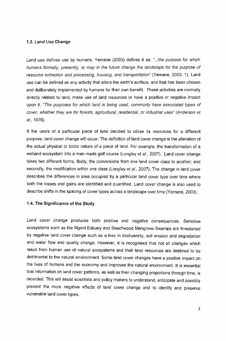
1.3. Land Use Change
Land use defines use by humans. Yemane (2003) defines it as: " ... the purpose for which
humans formally, presently, or may in the future change the landscape for the purpose of
resource extraction and processing, housing, and transportation" (Yemane, 2003; 1). Land
use can be defined as any activity that alters the earth's surface, and that has been chosen
and deliberately implemented by humans for their own benefit. These activities are normally
directly related to land, make use of land resources or have a positive or negative impact
upon it. "The purposes for which land is being used, commonly have associated types of
cover, whether they are for forests, agricultural, residential, or industrial uses" (Anderson et
al., 1976).
If the users of a particular piece of land decided to utilise its resources for a different
purpose, land cover change will occur. The definition of land cover change is the alteration of
the actual physical or biotic nature of a piece of land. For example, the transformation of a
wetland ecosystem into a man-made golf course (Longley et al., 2007) . Land cover change
takes two different forms, firstly, the conversions from one land cover class to another; and
secondly, the modification within one class (Longley et aI. , 2007). The change in land cover
describes the differences in area occupied by a particular land cover type over time where
both the losses and gains are identified and quantified. Land cover change is also used to
describe shifts in the spacing of cover types across a landscape over time (Yemane, 2003).
1.4. The Significance of the Study
Land cover change produces both positive and negative consequences. Sensitive
ecosystems such as the Mgeni Estuary and Beachwood Mangrove Swamps are threatened
by negative land cover change such as a loss in biodiversity, soil erosion and degradation
and water flow and quality change. However, it is recognised that not all changes which
result from human use of natural ecosystems and their land resources are destined to be
detrimental to the natural environment. Some land cover changes have a positive impact on
the lives of humans and the economy and improves the natural environment. It is essential
that information on land cover patterns, as well as their changing proportions through time, is
recorded. This will assist scientists and policy makers to understand, anticipate and possibly
prevent the more negative effects of land cover change and to identify and preserve
vulnerable land cover types.
3

This study seeks to identify whether land cover changes have occurred within and
surrounding the Mgeni Estuary and Beachwood Mangrove Swamps study area, and to
determine if these land cover changes have a negative or positive impact on these natural
ecosystems. In addition, the study aims to determine whether land cover change has
impacted upon wetland bird populations within these ecosystems. Birds are recognised as
an appropriate tool for monitoring the health and integrity of natural ecosystems throughout
Europe and the North America (US Environmental Protection Agency, 2007). However, the
utilization of birds as an environmental monitoring tool is a relatively new concept in
Southern Africa, and the study sought to reinforce the argument that wetland avian species
should be appropriately monitored to help assess the health and integrity of ecosystems in
terms of the negative impacts of land cover change within mangrove ecosystems, and within
the vicinity of water bodies and wetlands.
In order to determine the usefulness of wetland bird species as an effective monitoring tool ,
the CWAC Wetland Bird Census Database complied by the Animal Demographic Unit,
University of Cape Town was assessed, and indicator species for each land cover class
identified. Studies indicate that fluctuations in avian populations occurred due to negative or
positive land cover changes taking place within an ecosystem (US Environmental Protection
Agency, 2007). Fluctuations in avian populations within the study area could be due to
changes in land cover identified in archival aerial imagery. This would provide sufficient
evidence to conclude that wetland avian populations can be used as an effective tool to help
monitor the health and integrity of estuarine and mangrove ecosystems in Southern Africa.
1.5. The Importance of the Mgeni Estuary and Beachwood Mangrove Swamps
Estuaries and mangrove swamps perform various ecological functions as noted above. For
example, estuaries may be fringed by wetlands which fulfil a valuable role. By processing
water which drains from the uplands carrying sediments, nutrients and sometimes pollutants
are then filtered out by wetland habitats, which ensure that the water is clean and clearer
and not harmful to the natural environment and humankind. Mangrove swamps help to
protect land from soil erosion and the effects of coastal storm surges. They also provide a
natural means of controlling pollution by filtering out industrial and human waste. Mangrove
swamps perform the same functions as wetlands, acting as a natural buffer between the
land and ocean , helping to absorb flood waters and dissipate storm surges and prevent soil
erosion. These natural ecosystems provide an opportunity for tourism associated with bird
watching and other recreational activities whilst also supporting the fishery industry and
4
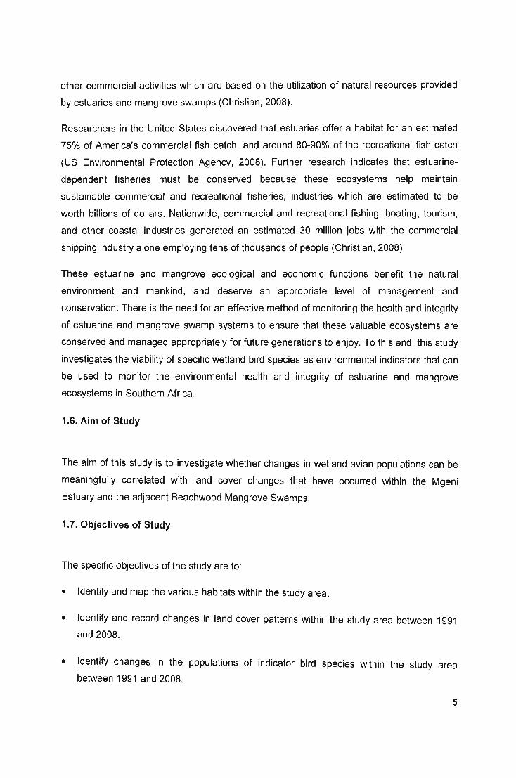
other commercial activities which are based on the utilization of natural resources provided
by estuaries and mangrove swamps (Christian, 2008).
Researchers in the United States discovered that estuaries offer a habitat for an estimated
75% of America's commercial fish catch , and around 80-90% of the recreational fish catch
(US Environmental Protection Agency, 2008). Further research indicates that estuarine
dependent fisheries must be conserved because these ecosystems help maintain
sustainable commercial and recreational fisheries, industries which are estimated to be
worth billions of dollars. Nationwide, commercial and recreational fishing, boating, tourism ,
and other coastal industries generated an estimated 30 million jobs with the commercial
shipping industry alone employing tens of thousands of people (Christian, 2008).
These estuarine and mangrove ecological and economic functions benefit the natural
environment and mankind , and deserve an appropriate level of management and
conservation. There is the need for an effective method of monitoring the health and integrity
of estuarine and mangrove swamp systems to ensure that these valuable ecosystems are
conserved and managed appropriately for future generations to enjoy. To this end, this study
investigates the viability of specific wetland bird species as environmental indicators that can
be used to monitor the environmental health and integrity of estuarine and mangrove
ecosystems in Southern Africa .
1.6. Aim of Study
The aim of this study is to investigate whether changes in wetland avian populations can be
meaningfully correlated with land cover changes that have occurred within the Mgeni
Estuary and the adjacent Beachwood Mangrove Swamps.
1.7. Objectives of Study
The specific objectives of the study are to:
•
•
•
Identify and map the various habitats within the study area.
Identify and record changes in land cover patterns within the study area between 1991
and 2008.
Identify changes in the populations of indicator bird species within the study area
between 1991 and 2008.
5

• Determine if there is a significant relationship between changes in the populations of
indicator bird species, and related changes in the patterns of land cover in the study
area.
• Identify the primary human activities that may have influenced estuarine and mangrove
habitats in the study area.
1.8. Structure of Thesis
Chapter Two, the Literature Review, examines estuarine and mangrove ecosystems within
South Africa, and the ecological and economic benefits they offer both local communities
and the natural environment. It explores the role of birds as environmental indicators and
bird adaptations to estuarine and mangrove habitats. In addition, this chapter investigates
land cover change in relation to estuaries and mangrove swamps in detail.
Chapter Three focuses on discussing the study area of the Mgeni Estuary and Beachwood
Mangrove Swamps ecosystem.
Chapter Four describes the Material and Methods, and provides an in-depth view into the
various data collection methods and procedures which were employed during the course of
the study.
Chapter Five presents the Results and Discussions.
Chapter Six, the final chapter, presents Conclusion and Recommendations.
6

Chapter Two
Literature Review
2.1 . Introduction
Estuaries and mangrove swamps are recognised as some of the most valuable ecosystems
on earth due to the variety of ecological and economic functions they perform. However,
many of these important ecosystems are now threatened by human expansion and
exploitation. Land cover changes around estuarine and mangrove ecosystems as a result of
human activities have a negative impact on the economic worth of such sensitive
ecosystems and consequently endanger their very existence. Land cover changes within
and surrounding the Mgeni Estuary and Beachwood Mangrove Swamps, have contributed to
the steady degradation and deterioration of foraging , roosting and reproductive habitats
utilised by wetland bird species. The sensitivity of wetland bird populations to habitat
transformation disturbances within estuaries and mangrove systems makes them an ideal
environmental indicator for monitoring the health and integrity of these valuable ecosystems.
Research has indicated that the disappearance of certain estuarine and mangrove habitats
has contributed to a decline in populations of wetland bird species within the Mgeni Estuary
and Beachwood Mangrove Swamps.
2.2. South African Estuaries and Mangrove Swamps
Day (1980) defined an estuary as, tt •• • a partially enclosed coastal body of water which is
either permanently or periodically open to the sea and within which there is a measurable
variation of salinity due to the mixture of sea water with fresh water derived from land
drainage" (Day, 1980; 2). This definition was adjusted by the compilers of the South African
National report to the United Nations Conference on Environment and Development which
was held in Rio de Janeiro in June 1992 (Day, 1980) and a new definition of an estuary
within a South African context was established Estuaries are part of a river system which
has, or can from time to time, be in contact with the sea. During periods of flooding , an
7
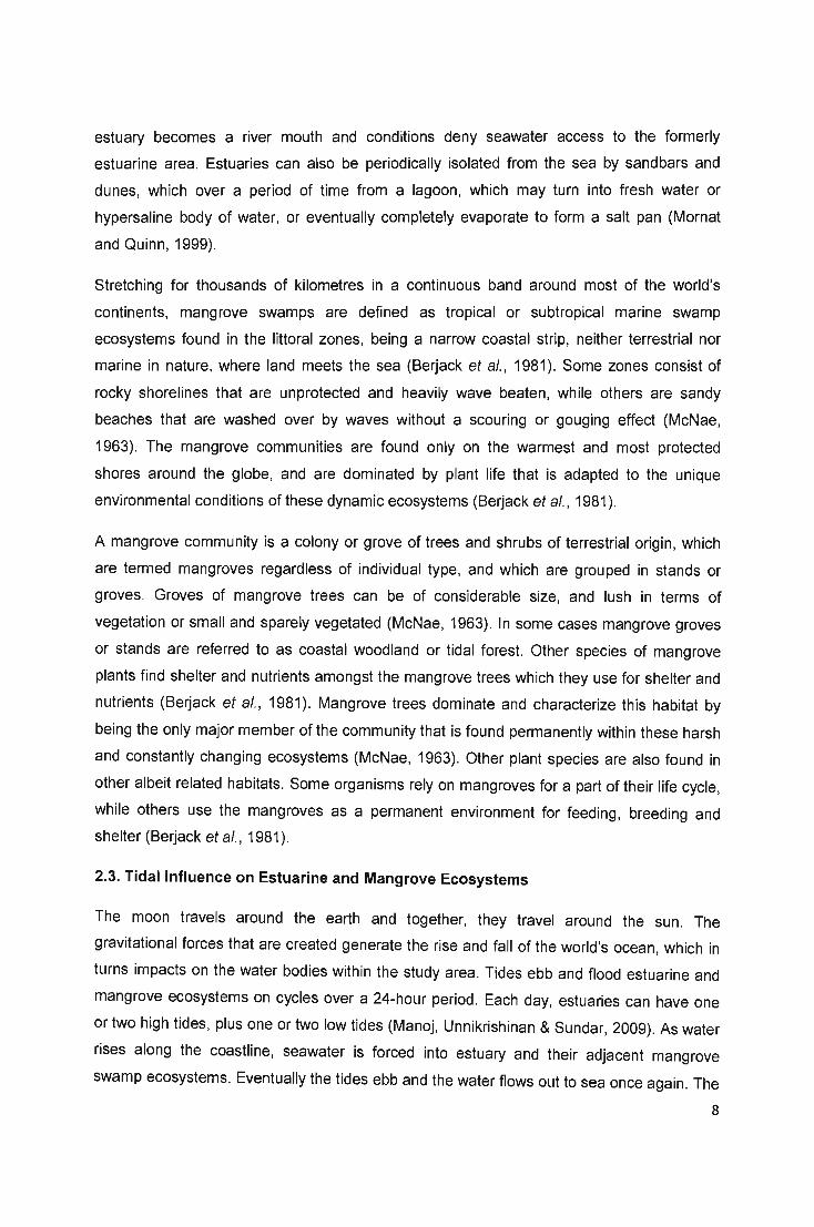
estuary becomes a river mouth and conditions deny seawater access to the formerly
estuarine area. Estuaries can also be periodically isolated from the sea by sandbars and
dunes, which over a period of time from a lagoon, which may turn into fresh water or
hypersaline body of water, or eventually completely evaporate to form a salt pan (Mornat
and Quinn, 1999).
Stretching for thousands of kilometres in a continuous band around most of the world 's
continents, mangrove swamps are defined as tropical or subtropical marine swamp
ecosystems found in the littoral zones, being a narrow coastal strip, neither terrestrial nor
marine in nature, where land meets the sea (8erjack et al., 1981). Some zones consist of
rocky shorelines that are unprotected and heavily wave beaten, while others are sandy
beaches that are washed over by waves without a scouring or gouging effect (McNae,
1963). The mangrove communities are found only on the warmest and most protected
shores around the globe, and are dominated by plant life that is adapted to the unique
environmental conditions of these dynamic ecosystems (8erjack et al., 1981).
A mangrove community is a colony or grove of trees and shrubs of terrestrial origin, which
are termed mangroves regardless of individual type, and which are grouped in stands or
groves. Groves of mangrove trees can be of considerable size, and lush in terms of
vegetation or small and sparely vegetated (McNae, 1963). In some cases mangrove groves
or stands are referred to as coastal woodland or tidal forest. Other species of mangrove
plants find shelter and nutrients amongst the mangrove trees which they use for shelter and
nutrients (8erjack et al., 1981). Mangrove trees dominate and characterize this habitat by
being the only major member of the community that is found permanently within these harsh
and constantly changing ecosystems (McNae, 1963). Other plant species are also found in
other albeit related habitats. Some organisms rely on mangroves for a part of their life cycle,
while others use the mangroves as a permanent environment for feeding, breeding and
shelter (8erjack et al., 1981).
2.3. Tidal Influence on Estuarine and Mangrove Ecosystems
The moon travels around the earth and together, they travel around the sun. The
gravitational forces that are created generate the rise and fall of the world's ocean, which in
turns impacts on the water bodies within the study area. Tides ebb and flood estuarine and
mangrove ecosystems on cycles over a 24-hour period . Each day, estuaries can have one
or two high tides, plus one or two low tides (Manoj , Unnikrishinan & Sundar, 2009). As water
rises along the coastline, seawater is forced into estuary and their adjacent mangrove
swamp ecosystems. Eventually the tides ebb and the water flows out to sea once again. The
8
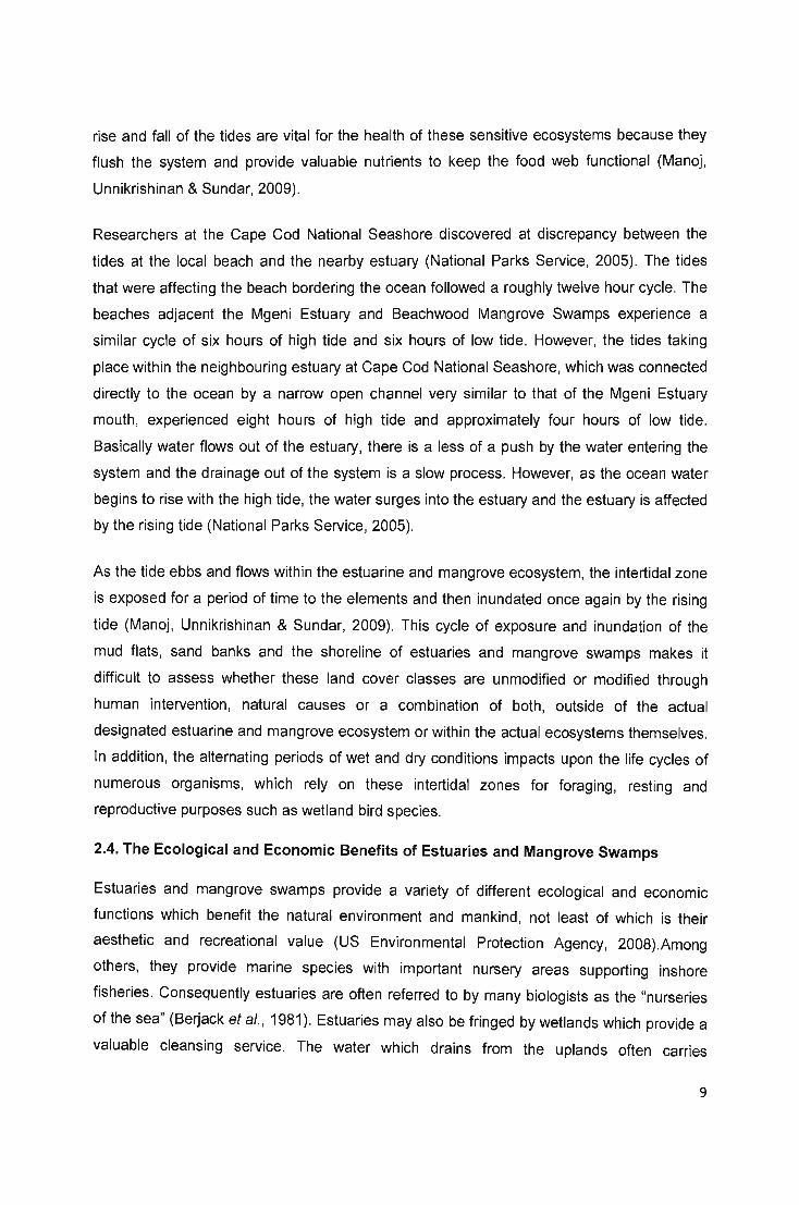
rise and fall of the tides are vital for the health of these sensitive ecosystems because they
flush the system and provide valuable nutrients to keep the food web functional (Manoj ,
Unnikrishinan & Sundar, 2009).
Researchers at the Cape Cod National Seashore discovered at discrepancy between the
tides at the local beach and the nearby estuary (National Parks Service, 2005) . The tides
that were affecting the beach bordering the ocean followed a roughly twelve hour cycle. The
beaches adjacent the Mgeni Estuary and Beachwood Mangrove Swamps experience a
similar cycle of six hours of high tide and six hours of low tide. However, the tides taking
place within the neighbouring estuary at Cape Cod National Seashore, which was connected
directly to the ocean by a narrow open channel very similar to that of the Mgeni Estuary
mouth, experienced eight hours of high tide and approximately four hours of low tide.
Basically water flows out of the estuary, there is a less of a push by the water entering the
system and the drainage out of the system is a slow process. However, as the ocean water
begins to rise with the high tide, the water surges into the estuary and the estuary is affected
by the rising tide (National Parks Service, 2005).
As the tide ebbs and flows within the estuarine and mangrove ecosystem, the intertidal zone
is exposed for a period of time to the elements and then inundated once again by the rising
tide (Manoj , Unnikrishinan & Sundar, 2009). This cycle of exposure and inundation of the
mud flats, sand banks and the shoreline of estuaries and mangrove swamps makes it
difficult to assess whether these land cover classes are unmodified or modified through
human intervention, natural causes or a combination of both, outside of the actual
designated estuarine and mangrove ecosystem or within the actual ecosystems themselves.
In addition , the alternating periods of wet and dry conditions impacts upon the life cycles of
numerous organisms, which rely on these intertidal zones for foraging , resting and
reproductive purposes such as wetland bird species.
2.4. The Ecological and Economic Benefits of Estuaries and Mangrove Swamps
Estuaries and mangrove swamps provide a variety of different ecological and economic
functions which benefit the natural environment and mankind, not least of which is their
aesthetic and recreational value (US Environmental Protection Agency, 2008).Among
others, they provide marine species with important nursery areas supporting inshore
fisheries. Consequently estuaries are often referred to by many biologists as the "nurseries
of the sea" (Berjack et al., 1981). Estuaries may also be fringed by wetlands which provide a
valuable cleansing service. The water which drains from the uplands often carries
9

sediments, nutrients and other pollutants (Christian, 2008). As this water moves through the
wetland areas such as swamps and salt marshes, much of the sediment and pollutants are
naturally filtered out.
Various characteristics make wetlands suitable for this function , including the lowering of
water velocity due to the low gradient of the slope combined with wetland vegetation helping
to suspend particles to be deposited. The anaerobic and aerobic processes, such as
denitrification and nitrification, the constant contact between water and sediment and, finally
the high organic content within wetlands, are ideal for the retention of heavy metals. The
wetlands filtration process naturally creates clean and clearer water, which in turn
contributes profoundly to the well-being of humans and marine life in general (McNae, 1963;
US Environmental Protection Agency, 2008) .
Mangrove swamps help protect coastal land from soil erosion and the effects of storm
surges. They provide a means of controlling pollution by filtering out industrial and human
waste. Scientists also believe that mangrove swamps perform similar functions to wetlands:
acting like a natural buffer between the land and ocean, absorbing flood waters and
dissipating storm surges. Mangrove tree root systems help remove sediment from run off
before it reaches the open water of the ocean, thereby preventing sediment from covering
and killing coral reef colonies. The removal of sediment also assists in the protection of
inland habitats within the estuary and river systems, as well as protecting valuable real
estate from storm and flood damage (McNae, 1963). Estuarine salt marshes and the grass
species that colonize these areas also playa vital role in preventing erosion and contribute
to the stabilization of the shoreline.
These ecosystems protect the coastal waters of estuaries and provide ideal locations for
important public infrastructure, forming natural harbours and ports which are vital for
recreation shipping, transportation and industry (US Environmental Protection Agency,
2008). Studies in the United States were undertaken to measure certain aspects of
economic activities attributed to estuaries and other coastal waters to help determine their
contribution to society. Researchers discovered that estuaries provide habitat for an
estimated 75% of America's commercial fish catch, and around 80-90% of the recreational
fish catch (US fisheries were vital for maintaining sustainable commercial and recreational
fisheries). These industries are estimated to be worth billions of dollars. Studies also
indicated that commercial and recreational fishing , boating, tourism, and other coastal
industries generated an estimated 30 million jobs nationwide, with the commercial shipping
industry alone employing tens of thousands of people (Christian , 2008).
10

The economic value of South African estuaries and mangrove swamps is currently being
investigated by the Percy FitzPatrick Institute of African Ornithology at the University of Cape
Town. The researchers considered the subsistence, property, tourism, nursery and
existence values of temperate estuaries in South Africa within the context of a Total
Economic Value framework (Turpie and MSc Class, 2005). Total sUbsistence value of
estuaries in South Africa ranged from zero to RSOO 000 per estuary according to the study
(Turpie and MSc Class, 2005). The findings concluded that the average total subsistence
value of an estuary within South Africa was around R70 000. It was also determined that the
total property value around estuaries was estimated to be worth R10.6 billion (a capital
value) . The study converted these values to an annual value akin to the income that is
generated by the South African property sector, and this translated to a total of
approximately R320 million per year (Turpie and MSc Class, 2005)
The study indicated that the majority of estuaries within South Africa had a tourism value of
between R 10 000 and R 1 million per annum. Retail and tourism sectors by comparison,
generated an estimated R2.0S billion in annual turnover (Turpie and MSc Class, 2005).
Estuaries provide nurseries for various commercially or recreationally valuable fish species,
valued between R 10 000 and R 1 million per annum (Turpie and MSc Class, 2005).
According to researchers, temperate estuaries generated R773 million. Researchers
explored the existence value of estuaries and the public's perceptions of such ecosystems,
indicating that many people were willing to pay R90 million for South African estuaries simply
because of the feeling of satisfaction that their existence generates (Turpie and MSc Class,
2005). Further research revealed that respondents tended to focus on scenic beauty and
biodiversity importance when they were asked to rate individual estuaries, but the scores
were very well correlated with the scenic value of these locations alone (Turpie and MSc
Class, 2005). This allowed researchers to extrapolate the scores of all other estuaries within
South Africa simply based on the independent rating of scenic beauty. The scores were then
used to disaggregate the overall WTP for all the estuaries within South Africa (Turpie and
MSc Class, 2005).
The study indicated that the poorest members of society tend to favour higher levels of
development around estuaries (average 4S%) compared to the wealthier members (average
25%). However, all respondents felt that at least 50% of these estuaries should remain intact
and undeveloped. Other researchers undertook a study to examine the economic value of
mangrove ecosystems within South Africa. A project examining the value of the Mngazana
Estuary Mangroves was conducted by the Percy FitzPatrick Institute of African Ornithology
(Schroenn, de Wet and Turpie, 2005). A partial economic valuation of the benefits that
11
mangrove ecosystems offer local rural communities was undertaken. The researchers
gathered data from the local communities surrounding the estuary undertaking household
surveys and holding focus group discussions (Schroenn, de Wet. and Turpie, 2005). A
market price method was applied to determine the value of mangroves that were harvested
for building material, and the subsistence consumption of fish by local communities living in
the vicinity of estuaries around South Africa (Schroenn, de Wet and Turpie, 2005). Various
other values were estimated such as honey production , canoe trails and finally the local
economic impact of expenditure of visitors utilizing local accommodation that is adjacent the
estuary. These results were then incorporated into a 20-year valuation model with the net
annual benefits, and then these were discounted to present value terms. The sensitivity
analysis was undertaken by the researchers to determine lower-bound, upper-bound and
most-likely values (Schroenn, de Wet and Turpie, 2005).
The Mngazana Estuary Mangroves had a minimum economic value between RO.5 and R7.0
million, at a most-likely value at a 5% discount rate of R3.4 million (Schroenn , de Wet and
Turpie, 2005). This study illustrates the importance of implementing policies for managing
environmental goods and services that are ecologically, socially and economically sound.
Schroenn, de Wet and Turpie (2005) state that an integrated approach to address the socio
economic needs of local communities has the ability to help protect environmental resources
for future generations to enjoy.
Estuaries and mangrove swamps are recognised as sensitive ecosystems that are
vulnerable to human development and pollution. The clearance of land for development and
agriculture around and within such ecosystems, increases sediment loads (McCally, 2007).
This increase in the sediment load impacts on the clarity of the water, as well as the nature
of the sediments and the rate of sedimentation taking place within these ecosystems. In
addition, the construction of dams and other man-made obstacles within a river's catchment
can contribute to a reduction in downstream flow and the sediment load reaching the estuary
(McCally, 2007).
Numerous studies have been conducted that examine the annual sediment yields of river
catchments before the construction of dams, and following the commencement of the
operation of these same dams. The Mgeni River had a sediment yield of approximately 1-6x
10* tonnes before the construction of the Inanda Dam (Garland and Moleko, 2000).
However, the construction of five dams within the catchment area has gradually reduced the
contemporary sediment yield to the coast over a period of time. The catchments area below
the four main dams that were completed prior to 1987 is estimated to be around 1700 Km2 ,
12

and the total sediment yield from this area was calculated to be around 0-5 x 10* tonnes per
year (Garland and Moleko, 2000) . The completion of the Inanda Dam in 1988 has only
exacerbated the situation by altering bed load transportation and deposition. After the
completion of the Inanda Dam, the mean annual discharge of the river was significantly
reduced (4%). The establishment of a water release policy also had a major impact on the
discharge regime which has led to an increase in discharge events (Garland and Moleko,
2000). Sediment continually builds up behind the dam wall, which has led to a notable
reduction in available downstream sediment. Whereas the volume of sediment within the
estuary has not changed since 1989, the sediment calibre has become much finer (Garland
and Moleko, 2000) .
Garland and Moleko (2000) also mentioned that without the natural replenishment of
downstream sediment from the upper reaches of the Mgeni Catchment area, sand mining
operations below the Inanda Dam will eventually cease. Such activities contribute to the
reduction in the amount of sediment being transported downstream towards the Mgeni
Estuary and the eThekwini beaches. Eventually, the estuary will begin to deepen, and the
mudflats and sand banks will gradually disappear as the coarse pre-dam sediment is
eventually flushed out into the Indian Ocean and is replaced by new sediment of a finer
particle size. Local eThekwini beaches will also be affected as their sediment supply is
curtailed. This process would have a considerable impact on the overall environmental
conditions of the estuary. Scientists have found that many different invertebrates, plants,
fish , birds and mammals prefer certain sediment particle sizes. Consequently, some might
be affected by even minor changes in the rate of sedimentation, and the level of turbidity and
either die out or relocate to more suitable habitats (EW Environment Waikato Regional
Council, 2007).
In some instances, other man-made disturbances can also result in greater sediment runoff
into estuarine ecosystems which can then increase the rate of estuary infill. The consequent
reduction in water depth can affect the distribution of plants, animals and their habitats, while
at the same time decreasing natural, recreational and amenity values (EW Environment
Waikato Regional Council, 2007). Fertilizers, pesticides and other toxic materials which are
washed into estuaries and mangrove swamps are also harmful to the balance of the natural
environment. Oil pollution can smother mangrove root systems and suffocate trees. The
development of infrastructure such as roads, railways and bridges increases the surface
runoff which carries sediment and pollutants into the estuary and mangrove ecosystems. As
coastal regions become more heavily populated , and the rate of development increases,
13
additional strain is put on ecosystems. Land is cleared for more housing and infrastructure.
Littering, results in increased incidents of resultant rubbish which washes into the estuarine
and mangrove ecosystem and damages vegetation (EW Environment Waikato, 2008).
Mangrove trees are sometimes cleared to supply timber, fuel or pulp. The World Wildlife
Fund has found that more than 35% of the world 's mangrove swamps have already
disappeared. In some countries such as India, the Philippines, and Vietnam this figure is
estimated to be around 50% (World Wildlife Fund, 2009). As such, it is clear that natural
estuarine and mangrove ecosystems are under threat.
2.5. Birds within Estuarine and Mangrove Ecosystems
Studies indicate that one hundred and sixty-two different species of birds are found within
estuarine and mangrove habitats around South Africa. As already stated , these bird species
are taxonomically, functionally and morphologically diverse. They range from piscivores,
such as White-Sacked Pelicans which can weight several kilograms, to small insectivores
like Sandpipers. Representatives of 13 of the 26 Orders of birds are found within South
African estuaries (Hockey et a/., 1992). The high taxonomic diversity of bird species in
estuaries can be attributed to the variety of diverse habitats which are found within the
estuarine ecosystems.
Several different habitat systems have been identified. These include shallow water, deep
open water, intertidal mud and sand flats, reed beds and mangroves, all of which are further
diversified by the existence of a strong salinity gradient which has a significant influence on
the spatial occurrence of plant and invertebrates (Kalejta and Hockey, 1991). Tthis habitat
diversity exists within restricted areas. Estuaries attract various bird species with their wide
range of habitat requirements for breeding , feeding and roosting . In six of the avian Orders,
more than two-thirds of the species are found regularly in estuaries. Whilst these Orders are
normally closely associated with aquatic habitats, they are not necessarily exclusively or
predominantly within estuaries (Kalejta and Hockey, 1991).
14
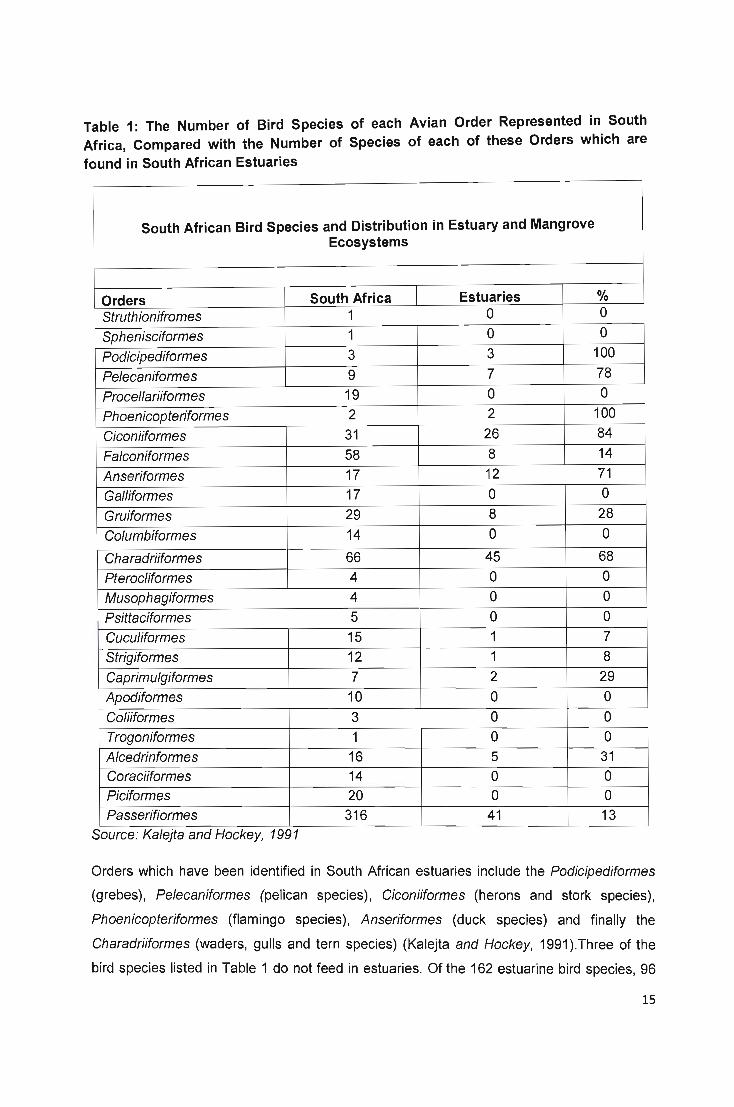
Table 1: The Number of Bird Species of each Avian Order Represented in South Africa, Compared with the Number of Species of each of these Orders which are found in South African Estuaries
South African Bird Species and Distribution in Estuary and Mangrove Ecosystems
Orders South Africa Estuaries % Struthionifromes 1 0 0
Sphenisciformes 1 0 0
Podicipediformes 3 3 100
Pelecaniformes 9 7 78
Procellariiformes 19 0 0
Phoenicopteriformes 2 2 100
Ciconiiformes 31 26 84
Falconiformes 58 8 14
Anseriformes 17 12 71
Galliformes 17 0 0
Gruiformes 29 8 28
Columbiformes 14 0 0
Charadriiformes 66 45 68 Pterocliformes 4 0 0 Musophagiformes 4 0 0 Psittaciformes 5 0 0 Cuculiformes 15 1 7 Strigiformes 12 1 8 Caprimulgiformes 7 2 29 Apodiformes 10 0 0 Coliiformes 3 0 0 Trogoniformes 1 0 0 Alcedrinformes 16 5 31 Coraciiformes 14 0 0 Piciformes 20 0 0 Passerifiormes 316 41 13
Source: Kale}ta and Hockey, 1991
Orders which have been identified in South African estuaries include the Podicipediformes
(grebes) , Pelecaniformes (pelican species) , Ciconiiformes (herons and stork species) ,
Phoenicopteriformes (flamingo species) , Anseriformes (duck species) and finally the
Charadriiformes (waders, gulls and tern species) (Kalejta and Hockey, 1991 ).Three of the
bird species listed in Table 1 do not feed in estuaries. Of the 162 estuarine bird species, 96
15
(59%) actually breed in estuaries. However, a few species migrate to the tropics during the
non-breeding season. Studies indicate that 66 species only visit estuaries to forage and
roost. Some of these visitors are long-distance migrants from Palaearctic breeding grounds
in the northern hemisphere (Kalejta and Hockey, 1991). Some species such as Flamingos
and Mangrove Kingfishers are intra-African migrants. Several researchers have shown that it
is not possible to give an accurate assessment of the total number of birds that actually
utilise South African estuaries because the abundance and composition of bird populations
are dynamic over time scales as short as hours, causing inaccuracies in counts. Secondly,
skulking species such as bitterns, rails and crakes, and nocturnal species such as owls,
night herons and night jars are not easily seen during surveys. Such species spend much of
their existence in structurally complex habitats such as reed beds.
The number of birds in estuaries fluctuates all year round; however, the most significant
changes in avifauna are seasonal. During the austral summer, hundreds of thousands
Palaearctic-breeding waders take up residence in South African estuaries. The first birds
arrive in August, and most have left by the end of May to return to northern breeding
grounds. Juveniles of most of the migrating wader species take up residence in South
African estuaries during their first year and remain throughout the Southern winter; finally
migrating north to their breeding ground at two years of age (Martin and Baird, 1988). The
number of juvenile birds present in South African estuaries varies from year to year. As the
Palaearctic-breeding migrants leave the South African estuaries, other groups of birds begin
to arrive. Researchers indicate that for example that the Berg River Estuary is dominated by
migrant wading bird species during the summer. However, when these bird species migrate
north during the autumn, they are replaced by resident waders and waterfowl which remain
in the estuary throughout the winter
2.6. Diet and Foraging Behaviour of Estuarine Bird Species
Estuarine bird species are specially adapted to the location and consumption of specific food
types. There are six major dietary categories have been identified amongst estuarine bird
species in South Africa. This diversity of dietary categories is due to the wide range of
habitats systems found within estuaries (Kalejta and Hockey, 1994). The aquatic and
terrestrial habitats of estuaries are rich with various different invertebrates, vertebrates and
plant types consumed by resident bird species. Within each of the thirteen estuarine bird
Orders, the species normally fall within one or two categories in terms of the main
components of their diet. Findings indicate that invertebrate feeders dominate in all estuarine
ecosystems within South Africa (Kalejta and Hockey, 1994)
16
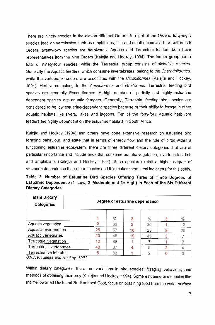
There are ninety species in the eleven different Orders. In eight of the Orders, forty-eight
species feed on vertebrates such as amphibians, fish and small mammals. In a further five
Orders, twenty-two species are herbivores. Aquatic and Terrestrial feeders both have
representatives from the nine Orders (Kalejta and Hockey, 1994). The former group has a
total of ninety-four species, while the Terrestrial group consists of sixty-five species.
Generally the Aquatic feeders, which consume invertebrates, belong to the Charadriiformes;
while the vertebrate feeders are associated with the Ciconiiformes (Kalejta and Hockey,
1994). Herbivores belong to the Anseriformes and Gruiformes. Terrestrial feeding bird
species are generally Passeriformes. A high number of partially and highly estuarine
dependent species are aquatic foragers. Generally, Terrestrial feeding bird species are
considered to be low estuarine-dependent species because of their ability to forage in other
aquatic habitats like rivers, lakes and lagoons. Ten of the forty-four Aquatic herbivore
feeders are highly dependent on the estuarine habitats in South Africa.
Kalejta and Hockey (1994) and others have done extensive research on estuarine bird
foraging behaviour, and state that in terms of energy flow and the role of birds within a
functioning estuarine ecosystem, there are three different dietary categories that are of
particular importance and include birds that consume aquatic vegetation, invertebrates, fish
and amphibians (Kalejta and Hockey, 1994). Such species exhibit a higher degree of
estuarine dependence than other species and this makes them ideal indicators for this study.
Table 2: Number of Estuarine Bird Species Offering Three of Three Degrees of Estuarine Dependence (1=Low, 2=Moderate and 3= High) in Each of the Six Different Dietary Categories
Main Dietary Degree of estuarine dependence
Categories
1 % 2 % 3 % Aquatic vegetation 5 63 2 25 1 13 Aquatic invertebrates 25 57 10 23 9 20 Aquatic vertebrates 20 48 19 45 3 7 Terrestrial vegetation 12 86 1 7 1 7 Terrestrial invertebrates 40 87 4 9 2 4 Terrestrial vertebrates 5 83 1 2 0 0
Source. Ka/e}ta and Hockey, 1991
Within dietary categories, there are variations in bird species' foraging behaviour, and
methods of obtaining their prey (Kalejta and Hockey, 1994). Some estuarine bird species like
the Yellowbilled Duck and Redknobbed Coot, focus on obtaining food from the water surface
17

while swimming while some species prefer diving to find food on the estuary bed. Waders
generally prey on aquatic invertebrates found close to the surface of inter-tidal mudflats by
pecking or shallow probing once the prey has been visually identified by the bird. However,
waders can also locate prey by secondary clues such as surface casts of poychaetete
worms and the movement of prawns as they irrigate their burrows (Smith, 1981). The range
of foraging habitats is limited by their morphology, as well as the range of prey they locate
and consume.
The Little Stint which is the smallest wading bird in South Africa has adapted to foraging for
its prey on exposed mudflats, salt marshes and along the water. Its legs are small and not
adapted to wading in deep water, and its beak is too short to probe very far beneath the
surface of the mud. Their small size allows Little Stints to forge on floating mats of algae and
other material. Scolopacid waders such as Curlews and Sandpipers have a larger body size
correlating with a larger beak and longer legs adapted to wading into deeper water (Kalejta
and Hockey, 1994). Longer bills allow these waders to probe deeper into the mud to catch
their prey. Like smaller waders , the scolopacid waders use their eyesight to visually identify
their prey, as well as using secondary clues
Black-Smith and Crowned-Plovers are exclusively visual foraging bird species with short bills
and legs which are not adapted to wading into water. The Pied, Giant and Mangrove
Kingfisher species either hover in the air above open water or the shallows trying to locate a
fish , before plunging at great speed into the water to catch their prey. The only filter-feeder
found in estuaries is the Greater-Flamingo which consumes crustaceans. Above the estuary,
swarms of mosquitoes, dragonflies and other invertebrates become the prey of Swallows,
Swifts, Martins and other bird species. The majority of the piscivores use one of three
techniques. Herons and Storks wade steadily through the shallows or deeper water, moving
their feet in the mud and vegetation on the estuary bottom to scare fish, amphibians and
other prey species out into the open. These species also practice a 'sit-and-wait' strategy to
catch unsuspecting prey along the water's edge (Hockey & Turpie, 1999). Generally when
the Heron spots movement of its prey below the surface, it plunges its beak into the water to
grab its victim. Cormorants and Darters dive beneath the water's surface and hunt for fish
amongst submerged logs and other obstacles below the surface. Pelicans swim along and
catch prey close to the water's surface.
Ecological segregation of bird species within estuarine environments has been researched
extensively around the world . The wide diversity of bird species that exist within many
estuarine ecosystems has the potential for inter-species competition for food. Kalejta and
18

Hockey (1994) state that there are several different mechanisms which can be employed by
different bird species to avoid competition with other species within the estuarine ecosystem.
These range from changes in bird behaviour, physical characteristics and possibly prey
types. Kalejta and Hockey (1994) states that birds have options which include where to feed,
when to feed and how to feed, what to actually eat.
Velasquez and Hockey (1992) state that there are even differences in foraging habitats at
the macro scale between species within a particular diet category. Studies which were
conducted at various different estuaries around South Africa during the 1980s and 1990s
examined the competition between different estuarine species. For example, at the Berg
River estuaries, the majority of waders forage on the exposed mudflats of the estuary, where
as Ruffs tend to favour salt marshes, as do the herbivorous Redbilled Teals (Velasquez,
Kalejta and Hockey, 1991). There are also differences between the foraging habits at the
meso-scale between different types of mudflats within the estuary systems.
An interesting example is the Ringed and Whitefronted Plovers which both inhabit the Berg
River Estuary. The Ringed Plovers tend to be found foraging in the areas of the estuary with
soft, fine mud while the Whitefronted Plovers tend to prefer the more sandy areas.
Velasquez and Hockey (1992) continue by discussing how wading piscivores, which inhabit
the St Lucia Estuary tend to avoid other species by segregating themselves spatially. This is
done by foraging in water of differing depths. For example, whilst White Egret tends to
forage in shallow water of an average depth of 100mm, the larger Greater White Egret will
wade into water with an average depth of 160mm. The world's largest heron, the Goliath
Heron, can be found foraging in water of a depth of 325mm (Velasquez and Hockey, 1992).
The intertribal mudflats are also exploited in three different dimensions by estuarine bird
species. The short-billed species tend to forage for food on the surface of mudflats, or probe
just below the surface of the mud, whereas longer billed species tend to obtain their prey
from a couple of centimetres below the surface (Hockey & Turpie, 1999). Evidence suggests
that the temporal segregation of the foraging activities of bird species in estuaries can
reduce interference competition; it will not reduce exploitative competition. Kalejta and
Hockey (1994) define exploitative competition as follows:
Exploitative competition occurs when the numbers of birds results in the depletion of
prey resources available to individuals to the point where availability is limited.
Interference competition occurs when birds directly hinder one another's access to
food, either by affecting prey behaviour or by restricting their space available in which
to gain access to resources (Kalejta and Hockey, 1994; 242).
19
The tidal rise and fall that occurs within open estuaries puts severe restrictions on the time
available for bird species to access their food source inter-tidally. Tidal variation expands
and contracts foraging habitats and has a significant influence on predation dynamics in the
estuary itself. This has an impact on the extent to which temporal segregation of foraging
can be employed by birds (Hockey et a/. , 1992). Some bird species are forced to forage both
day and night because of a restricted day-light foraging time.
The wading piscivorous species are not affected by tidal variations and the limited time
available to forage in the estuarine environment. The Herons, Egrets and Storks are able to
forage at both high and low tide because of their longer legs. The majority of wading
piscivorous species are daytime foragers, returning to communal roosting sites during the
evening. Ornithologists have seen Goliath and Grey Herons foraging both night and day
along the shores of Lake Turkana, Kenya (Hockey et al., 1992).
2.7. Birds as Indicators of Environmental Change
Ornithologists and scientists have begun to recognize the importance of using birds as
environmental indicators. Birdlife International, a global partnership of conservation
organisations which strive to conserve birds, their habitats and global biodiversity, stress that
birds must be recognised as valuable indicator species for biodiversity conservation.
Birdlife International state that birds are ideal indicators because they have widespread
popular appeal, and they make ideal flagship species for rallying and mobilizing volunteer
based monitoring networks and programmes, as well as for education and advocacy within
civil society (Birdlife International, 2008). Furthermore, birds are highly sensitive to many
environmental disturbances. Scientists can monitor the environmental health and integrity of
an area and identify potentially harmful changes within the environment by using birds as
indicators. Birds are found in a broad range of ecosystems, have varied natural histories,
and are found in all regions and countries around the world. Biologists state that birds are
high up the food chain, thus integrating changes at lower tropic levels and they are the best
known and best-documented major taxonomic group. This is true in terms of the sizes and
trends of populations and their distribution, and the number of species (c.10 OOO) is
manageable. This allows for comprehensive and rigorous analyses (Birdlife International,
2008).
The US Environmental Protection Agency has utilized birds as indicators of environmental
health and integrity over the last two decades. In the early 1990s a study was undertaken by
20

the US Environmental Protection Agency to determine whether birds could be utilized as
indicators of prairie wetland integrity. The researchers believed the following factors made
birds ideal for monitoring wetland integrity and health. Firstly, birds are easy to monitor
(usually no samples to process) and secondly, identifying birds is a simple task and can be
undertaken by capable non-scientists who are willing to assist with surveys (Crewe and
Timmermans, 2005). In addition, established survey protocols are readily available. Some
species have the tendency to accumulate toxic substances within their bodies because of
their position at the right end of the food chain . Birds are also useful for situ assessments
(confined or behaviourally imprinted individuals) (Morrison , 1986). Many bird species have a
longer lifespan than other bio-indicators which make them far more sensitive to cumulative
impacts and more able than other groups to integrate the effects of episodic events
(Morrison, 1986). Researchers all indicate that the ease of access to a relatively extensive
nationwide database on avian trends, habitat needs and distribution and finally the
availability of moderately extensive bioassay data base, all combine to make them
favourable environmental indicators (Crewe and Timmermans, 2005). Some species of birds
will leave an area, or modify their behaviour within an area, to avoid the presence of
humans. Human over-utilization of an area elicits a variety of responses from the birds in the
area. These include bird communities changing in terms of species composition and density
as pastures are replaced by natural forests, and again as the pastures are replaced by
suburbs (Conway and Timmermans, 2005). Birds are influenced by natural phenomena as
well as human activities, and serve as useful gauges of habitat quality.
Several studies have been conducted using birds as indicators of environmental health and
integrity. Ornithologists in the United States indicate that half of the 700 species of birds
which have been recorded within the United States spend two-thirds of the year in the
tropical forests of Central, South America or the Caribbean islands (Miller, 2004). During the
warm summer months, when insects are plentiful, they return to North America to breed. A
United States Fish and Wildlife study, which was conducted between 1978 and 1987,
indicated that populations of 44 of the 62 surveyed species of insect-eating, migratory
songbirds in North America were declining. Figures indicated that 20 of the bird species
surveyed showed a decline of 25-45% (Miller, 2004). Further research indicated that habitat
destruction and fragmentation were the main reasons for this drastic decline in bird
populations. The destruction of the rain forests of South America for timber and agricultural
land was identified as one major problem. As a result, migrating bird species were losing
their winter habitats.
21

Secondly, the fragmentation of migrating birds' summer forests and grassland habitats in
North America due to the expansion of urban areas and agricultural activities has
fragmented once pristine forests and grasslands (Miller, 2004). A study was undertaken to
examine the shifting seabird distribution which was directly linked to the rapidly changing
marine environment in the Western Arctic (Oivoky, 1998). According to marine ornithologists
there are ten different ways that seabirds can serve as indicators: Indicators of meso- and
large-scale marine habitat characteristics; ecosystem controls; temporal environmental
variation and climate change; zooplankton and fish stocks; fish and zooplankton
communities; contaminants; harmful algal blooms; fisheries and other human impacts on
marine ecosystems; and finally of fisheries management and ecosystem-based
management in general. The Bering Land Bridge acted as an impassable barrier to the
dispersal of seabirds on the Bering/Chukchi Shelf until approximately ten thousand years
ago (Oivoky, 1998). In the last four decades significant changes have occurred in the Arctic
Basin, which have resulted in a decrease in the latitudinal environmental gradient in the
entire region. The Chukchi Sea does not have an active commercial fishery and systematic
biological sampling, which means that the changes in seabird distribution and abundances in
the area are the most effective means of measuring the timing and magnitude of ongoing
climate change (Oivoky, 1998).
Researchers indicated that three different species of seabirds have shown significant signs
of range expansion and population increase. These are both species of Puffin which are now
occupying vast colonies throughout northern Alaska where they previously never existed;
and the population explosion of Bering Sea Alcids on the northern shelf (Oivoky, 1998).
However, research has also revealed that cold water species of seabirds such as Black
Guillemots (Cepphus grille) and Kittlitz's Murrelet (Brachyramphus brevirostris) appeared to
be decreasing in number due to the melting of the pack ice due to the rapid warming of the
ocean in the region (Oivoky, 1998). The findings of the research clearly indicate a link
between the warming of the Arctic Ocean and the distribution and abundance of different
species of seabirds in the Arctic.
For many decades marine ornithologists have argued that seabirds are good indicators of
the environmental health of ecosystem constituents (Furness & Tasker, 2000). Researchers
state that as the interest in the development of different approaches to marine conservation,
such as ecosystem management and ecosystem based approaches to fisheries
conservation grows, there has been an awakening interest in using seabirds as
environmental indicators, and their potential application to management sciences has been
recognised.
22

2.8. Avian Census Data and its Contribution to Environmental Monitoring
As already noted, avian indicators provide environmental agencies and organizations with an
effective tool to monitor diverse and sensitive ecosystems in an unobtrusive manner. One
such approach pioneered in the United States of America and Europe, is the identification
and examination of the fluctuations in wetland avian populations found within readily
available archival avian census data.
The avian census databases of the British Trust for Ornithology is regularly utilised during
environmental assessments throughout the British Isles (Hill et al., 1993). This data is
collected through annual surveys conducted by birders, volunteers and government officials
(Peakall, 2004). Avian census data provides conservation organisations and government
departments with an effective monitoring tool to manage agricultural production and industry
and its effects on avian populations. Surveys such as the Ringing Scheme provide valuable
information about the annual mortality rate of birds throughout the British Isles, the Common
Birds Census coordinate surveys and compiles field data about bird numbers into a
comprehensive and easily assessable index and the Constant Effort Sites monitors the
productivity and survival rate of specific bird species (Peakall, 2004) . British scientists have
also begun to monitor these databases in an attempt to help monitor global warming .
Avian census data is collected on an annual basis in several states around the United States
for lagoons, estuaries, lakes and river systems by NGOs, government agencies and private
groups and individuals to gauge the health of bird populations, as well as the overall health
of these ecosystems (Canterbury et al. , 2000). The archival avian census data that is
currently available for estuarine ecosystems is extensive and regularly up-dated. The
importance of such census databases has been recognised by several government agencies
such as the United States Environmental Protection Agency (Wheeler, 2008). These
organisations regularly utilise this data when assessing the health and integrity of water
bodies throughout the United States. The examination of avian census data contributes to
the overall assessment of the health and integrity of a wetland or estuarine ecosystems.
Meanwhile, in South Africa the collection of wetland avian census data is a recent
phenomenon. Prior to the establishment of the Coordinated Waterbird Counts (CWAC)
project in 1992 by the Animal Demography Unit (ADU) of the University of Cape Town ,
wetland avian data was collected in an ad hoc and unregulated manner by random
individuals and bird clubs (Wheeler, 2008). Some data was compiled into a useable
database and much of it was lost. The Coordinated Waterbird Counts (CWAC) project
23
coordinates, prioritise and continues to expand waterbird surveys on a national level with a
focus on the establishment of an effective long term waterbird monitoring tool that can
benefit conservation efforts at a local and global level. The project ensures that data is
effectively and efficiently compiled, managed and shared amongst conservation bodies and
the general public (Allen, 2008).
Since 1992, regular six monthly counts of all major water bodies have been undertaken by
volunteers and several organisations with a passion for waterbird conservation . This has
assisted in the creation of a concise wetland avian census database. The Coordinated
Waterbird Counts (CWAC) project is currently one of the largest and most successful citizen
science programmes on the African continent (Wheeler, 2008). The project is responsible for
the monitoring of over 400 wetland ecosystems from all over South Africa, and also curates
waterbird data for over 600 different sites (Wheeler, 2008).
Local ornithologists indicate that the collection of waterbird data from around South African is
vital because it provides an indication of the seasonal movements and the relative
importance of sites for the protection of different species through the comparison of counts
from different locations. Wheeler (2008) states that the long term monitoring of the numbers
of wetland birds utilising a particular location allows for the development of an annual
population indices which can be used to trace fluctuations of these populations over a period
of time. These counts provide a better understanding of how wetland bird species actually
use wetland habitats. It helps identify which locations are of particular importance to the
survival of wetland bird populations, and it helps in the provision of information support for
the development and implementation of management policies and it also provides an
effective means of monitoring the health and integrity of the wetland ecosystem as a whole
(Allen, 2008).
The emphasis of this study is to assess and process all the bird count data collected by
volunteers and birders during their six-monthly visits to the Mgeni Estuary and Beachwood
Mangrove Swamps since 1992, as compiled and published by the Coordinated Waterbird
Counts (CWAC) project for utilisation by government organisations and private individuals
for studies such as this. The fluctuations in wetland bird populations since the beginning of
official bird counts was statistically correlated with land cover changes identified through the
analysis of aerial imagery in order to determine if fluctuations in the number of birds
recorded within the study area could be directly linked to alterations in land cover within a
predetermined time period.
24

2.9. Using Birds as Environmental Indicators in Estuaries
As ecosystems around the globe become increasingly affected by human activity, the need
to monitor, evaluate, manage and remediate the ecological impacts of these changes
becomes even more vital. Because of the complexity of these ecosystems, such as
estuaries and mangrove swamps, it is likely that the use of biological indicators will also
increase. The use of bioindicators has dramatically increased over the last couple of
decades, and several environmental agencies in the United States have adopted colonial
waterbirds as a tool for helping to monitor water bodies such as estuaries, lagoons and river
systems (Kushlan, 1993).
Colonial waterbirds are recognised as the best documented and most reliable bioindicators
for the monitoring of the health and integrity of estuarine and mangrove ecosystems
because of the following :
• Aspects of colonial waterbird biology.
• The extent of biological understanding of that biology.
• The interest of humans in colonial waterbirds.
• Historical Precedent.
As already stated above, water birds are highly visible, sensitive to environmental changes
in both nesting and feeding habitats, and are positioned high up on the food chain (Kush lan,
1993}.For example, if scientists noticed a decline in the numbers of water birds species
which feed at the marsh-bay interface, this may indicate a reduction in tidal marsh habitat
due to sand mining and the reduction in the quality of the habitat by the spillage of crude oil
or the decline or disappearance of prey species (Slack, 1992). The decline of Northern
Pintails and Green-Winged Teals in the Galveston Estuary area of Texas could be closely
linked to environmental degradation that was occurring beyond the estuary itself. However,
research has indicated a sharp decline in non-migratory bird species such as the Mottled
Duck. Slack (1992) stated that this was probably due to salt water moving into the duck
nesting habitats.
A study entitled, "Status and Trends of Selected Vertebrate Resources in the Galveston
Estuary: Birds and Alligators" indicated a decline in the total number of several water bird
species which inhabit and visit the Galveston Estuary during migration (Slack, 1992). The
findings also revealed a steady decrease in the number of birds per colony within the same
25

species. The data used to generate the visual representation of this decline was provided by
the Texas Colonial Waterbird Survey (Slack, 1992). Certain species of waterfowl such as the
Mottled Duck (Anas fulvigula) , Northern Pintail (Aanas acuta) and Blue-Winged Teal (Anas
discors) also showed a steady decline in abundance in the Galveston Estuary area as
indicated by the Mid-Winter Waterfowl Transects. These transects reflected a widespread
trend which has caused serious concern amongst conservationists and ornithologists alike
on a national level (Hill et al., 1993).
Slack (1992) undertook another study which focused on the Texas Colonial Waterbird
Survey. This data was considered the most robust data set available on estuc;lrine bird
species in the United States (Slack, 1992). Furthermore, this data did not indicate any
significant trend in the total number of water birds and no mention was made of a trend in
species richness from 1973 to 1990. As Slack (1992) stated, "". a detrended
correspondence analysis (using the methodology of Spendelow et al. 1989) revealed
significant changes in species and habitat associations" (Slack, 1992; 2). All the birds which
showed similar population trends were selected and allocated into three different groups,
each group with its similar feeding habitats. These three groups were as follows:
Inland Group (little Blue Herons, White Ibises, Cattle Egrets, White-Faced Ibises and Great
Blue Herons) consists of freshwater marsh feeders and generalists. There was no evidence
provided by the study to indicate a decline in the number of individuals or the percentage of
them in the community over all (Slack, 1992). However, the study clearly showed that the
number of bird colonies in the estuary had increased, but those colonies where these
species were present showed that their proportion in the colony had decreased.
The Open Water Group (Royal Terns, Cormorants, and Sandwich Terns) is basically made
up of open-bay fish eating bird species. According to the study these species showed a
remarkable increase in numbers of individuals, the number of colonies and the number of
them in the overall estuarine community (Slack, 1992).
The Marsh Group (Snowy Egrets, Black Skimmers, Spoonbills and Great Egrets) which are
all species of water birds which consume small fish and other organisms at the marsh-bay
interface. This group showed a steady decline in total numbers and the proportion that they
composed in these colonies where they occurred. The number of colonies which contained
these species increased but the mean colony size decreased. Slack (1992) mentioned that
certain species of water birds were outliers in this analysis. For example, the Least Terns
were considered as opportunistic nesters and strictly colonial. The researchers also
26

classified laughing gulls as generalists. According to the survey data, the gulls showed no
population trend and no decline in their population .
After carefully analysing the findings of the study, it was concluded that feeding habitat, and
not nesting habitat, was the main controlling factor in the trends observed, because most of
the water birds species actually nested together in the same colonies (Kushlan , 1993). The
steady decline in the numbers of marsh-feeding birds in the estuary correlated with the loss
of wetland habitat. Although the nesting habitat was not considered the controlling factor in
the estuary it is more important on a local scale. There is plenty of documented evidence of
entire rookeries being lost to subsidence or erosion. Human activities in the estuary have
caused birds to desert their nests, leaving their eggs and chicks exposed to predators and
the elements. Invasions of fire ants have also been observed. The findings of the study
indicated that nesting habitats are important, but are not the driving force of the estuary-wide
trend (Kushlan , 1993).
Several possible causes for the decline in the estuarine bird species in the Galveston
Estuary were listed by Slack (1992). The first suggestion presented by the researchers was
the decrease in the quality of the feeding habitat. Other possibilities could be the existence
of pollutants which are concentrated in the water of the estuary, sediments or the prey
species which are consumed by the wetland bird species. Water birds are very effective
bioaccumulators of a wide variety of contaminants. Buoyant materials such as oil and
grease, tend to concentrate within the intertidal areas of estuaries and lagoons and this can
be detrimental to wading birds and skimmers. Oil spills are a serious problem around the
world and have a tremendous negative impact on an estuarine or mangrove ecosystem. Oil
and grease also form part of the non-point source pollution, and are often accidentally
released during activities relating to the movement of oil products (Kushlan, 1993). In
addition , effluent released by local factories can also lead to estuarine and mangrove
contamination (Berjack et a/., 1981).
A decline in the food supply also had a negative impact on bird populations. Researchers
found that an increase in death rate/morbidity could also threaten wetland bird species
because of disease or increased predation. This could be a natural occurrence or it could be
aggravated by human activity in the estuary (Conway and Timmermans, 2005). Another
problem is the decrease in the quality or quantity of nesting habitats. A colony could be
affected by inundation and erosion because of rising sea levels, wetland drainage or
sedimentation could create a land bridge between island colonies and the main land allowing
easy access to people and land-based predators (Kushlan , 1993). A build up of guano on
27
plants in an area which is harbouring more birds than is can cope with, gradually kills off
island vegetation. Normal succession could also deny bird species nesting sites. Increased
predator density with the introduction of dogs, cats , rats and other vermin also have an
impact. Direct disturbance by humans of nest sites could also lead to a decline in the
number or size of bird colonies. All these factors have an impact at local level. These would
all be expected to affect all water birds that nest together, not just those with similar feeding
habitats.
2.10. Assessment of Land Cover Changes
As already mentioned, estuaries and mangrove swamps are recognised as some of the
most valuable habitats on earth because of the variety of ecological and economic functions
they perform. However, estuaries and mangrove swamps are threatened by human
expansion and exploitation as manifested by land cover changes within and surrounding
these ecosystems. Land cover changes can either have a desirable or undesirable effect on
natural ecosystems. These sensitive ecosystems face a bleak and uncertain future without
an effective means of identifying, monitoring and managing land cover changes. The
assessment of land cover changes and correlating such changes against fluctuations in
wetland bird populations could be a useful environmental management tool to help assess
the environmental health and integrity of these estuarine and mangrove ecosystems.
The objective of a land cover change assessment is to record and portray changes that have
occurred over time. Langran (1993) indicated that change implies that there is a difference in
the land surface of a site between two dates, but also that this difference is uncharacteristic
of the normal circumstances that would be found from one time period to the next.
Assessments are undertaken by comparing the visible changes within an image of a
particular location , captured at a particular moment in time, against another image of that
same location at a completely different moment in time (Longley et a/., 2007) .
Academics refer to land cover changes observed as the change in the state of one or
several locations, entities, or both (Peuquet, 1999). Land cover changes occur at different
rates for various different locations and entities. Changes in land cover are not easy to
detect and measure. In some cases these differences are readily measured, the substantial
issue being that true change from what is perceived to be the normal environmental
variability and the artefacts of the processes of measurement (Longley et a/., 2007;
Eastman, McKendy and Michele, 1995).
28

Time series analysis is a process of examining changes over a sequence of images and
maps that represent land cover. This does not only focus on the perception of trends in
terms of changes but also describes the characteristic values and the abstraction of
anomalies from the series of imagery and maps (Longley et a/., 2007). According to Peuquet
(1999) and Veldkemp and Lambin (2001) there are no standards that are appropriate for
change and time series analysis. Some techniques focus on assessing the rate at which
change occurs, while others might put more emphasis on the spatial patterns (Peuquet,
1999, Veldkemp and Lambin, 2001) .
Any assessment involving changes in land cover will require the enhancement of remotely
sensed data quality and other ancillary data to ensure that the desired land cover information
is obtained. Data collected through remote sensing has no purpose by itself, because it
cannot be used to identify land cover types correctly. It is essential that a range of other data
be collected by the researcher, and this data should be combined with remote sensing data
to enhance the quality of this set data through the application of technologies such as GIS in
land cover change studies (Longley et a/., 2007) .
GIS is defined as a computer-based technology and methodology that is used to collect,
manage, analyze, model and present geographic data for a variety of applications such as
land cover assessments (Davis, 2001). This consists of three integrated elements which are
described as
• Geography: This is the real world or spatial realities.
• Information: The data that is collected and the information that is produced, their
interpretation and various uses.
• Systems: The computer technology and the supporting infrastructure.
GIS has numerous functions such as the collection of data from various sources, including
the global communications media. Data can be collected by remote sensing satellites,
collecting GPS coordinates in the field and via the internet (Longley et a/., 2007). It can be
easily retrieved simply by selecting and viewing the data on a computer screen , printed
maps, and the internet. It can be used to change and alter data from one form to another or
one map format to match another and can be an efficient digital storage system which allows
for administration and keeping track of data. GIS technology analyzes data to produce better
insight and new information using various different techniques such as data investigations,
statistical analysis procedures and other methods and finally it presents the data in maps,
graphs or reports that are easy to understand and reproduce (Longley et a/., 2007). GIS
29

assists with land management throughout South Africa because of its use as a decision
supporting tool and it has been used to map land use patterns throughout the region (Rivers
Moore, 1997). GIS is a vital asset because it enables many different role players to have the
opportunity to make better-informed decisions on the management and use of geographic
resources at their disposal (Yemane, 2003). Most land cover change studies in South Africa
utilise GIS technology as the tool to map and manipulate land cover databases (Yemane,
2003). GIS technology provides scale-free registration procedures and a wide variety of
analytical features that can assist researchers with the tools that are required to identify,
map and analyse the gradual disappearance of a particular land cover type within a specific
study area.
GIS can playa critical role in assessing land cover changes that are taking place within and
surrounding the Mgeni Estuary and Beachwood Mangrove Ecosystems. These ecosystems
are already showing visible signs of stress due to human expansion and exploitation that is
causing land cover change within and surrounding the study area. GIS technology provided
the researcher with a modern, efficient and reliable system to compile and manage field
data, aerial imagery and other data relating to land cover changes that are being identified
and investigated, retrieve and manipulate the data when necessary. Careful analysis of the
data will eventually allow for the presentation of the data of the study area in graphic and
tabular forms. This process will assist in a better informed decision making process
regarding land management within and in the vicinity of delicate ecosystems such as
estuaries and mangrove swamps. The findings of the research will be compared against the
findings of the analysis of the fluctuations of wetland bird populations identified in the CWAC
Bird Census data.
2.11. Summary
Land cover change within and surrounding estuarine and mangrove ecosystems can
produce both desirable and undesirable impacts. Sensitive ecosystems such as the Mgeni
Estuary and Beachwood Mangrove Swamps that provide the local community and the
natural environment with numerous ecological and economic benefits are threatened by
undesirable land cover changes and require rigid preservation and appropriate land
management. It has been proposed that the decline in the quantity and quality land covers
(habitats) within and surrounding the Mgeni Estuary and Beachwood Mangrove Swamps
due to human and natural causes, has had a negative impact on wetland bird populations.
According to numerous ornithologists, birds are highly sensitive to environmental
30

disturbances. Such disturbances include human induced land cover changes within
estuarine or mangrove habitats. Scientists around the globe have successfully used bird
species to monitor the health and integrity of the natural habitats, and have used bird
species to identify potential harmful changes. The assumption is that as the quantity and
quality of specific land cover types (e.g. mudflats, grassland) decline, then the populations of
wetland bird species that are adapted to foraging, nesting and roosting in these land cover
types will also show signs of decline.
31

3.1. Introduction
Chapter Three
Background to Study Area
Durban is a sub-tropical city on the east coast of South Africa. The Mgeni River flows
through the northern half of the city into the warm Indian Ocean. The study area comprises
the last 3 km of the river estuary and the adjacent mangrove swamps.
3.2. Background
The indigenous Zulu people, who inhabit the South African province of KwaZulu-Natal
named the river that flowed from the Drakensberg Mountains through the hills of the
hinterland through the estuary into the Indian Ocean, the Mgeni. Mgeni means "the river,
which flows through the thorn trees or Acacia" (Gillard , 2008) . The Mgeni River flows into the
Indian Ocean approximately 5 km north of Durban City centre at 29°48'S and 31°02'E. The
river and the estuary that form the Mgeni River mouth are surrounded by the northern
suburbs of Durban.
Mpumalanga
F ree State
Eastern Cape
Indian Ocean
,"-,>d
_ Reee anlh Aiea t~ Major TO'Mls
- National Routes o Local Munlc:lpaWd ••
OistrJct Municipalltie8 o Eastern Cape CJ Fr •• Stat. r-J ~mal .... ga c:::J LESOTHO
MOZAMBlaUES SIIIU\ZJLAND
Plate 1: The Study Area in Relation to KwaZulu-Natal (See Appendix A)
32

The Mgeni Estuary and Beachwood Mangrove Swamps are situated on the wave dominated
coastline and they occupy a narrow bedrock confined alluvial valley. The estuary is referred
to as a river dominated system due to the closing of the outlet by an elongated sand barrier.
The south bank of the estuary is protected from wave action by a groyne, which also acts as
a buffer to disrupt the deposition of long-short drift transported by the north-bound longshore
current (Begg, 1978). This prevents the estuary outlet closing permanently. Before the
construction of the Inanda Dam in 1985, the estuary mouth was permanently open because
the river flushed out any material which settled in this area (Plate 2). Garland and Moleko
(2000) indicated that the Inanda dam is holding back large quantities of water and sediment
which has now caused the river mouth to be a temporarily open-closed estuary. The
reduction in water volume and the progressive elongation of the barrier at the mouth of the
estuary have been identified as the primary causes of the temporary blockages at the
estuary mouth (Gillard, 2008). The study area which forms the basis of this study stretches
from the Connaught Railway Bridge to the estuary mouth which enters the Indian Ocean as
seen in Plate 2 (Gillard, 2008).
Plate 2: Mgeni Estuary Mouth
3.3. Mgeni Catchment and Estuary
The Mgeni Catchment area covers an estimated 4871 km2 (DEAT, 2001). The mean winter
and summer flows are 6.5 ms-1 and 18.4 ms-1 respectively. The lowest flow ever recorded
was 4, 5 ms-1
while the highest recorded flow was 532 ms-1 (Begg, 1978). Studies indicate
33
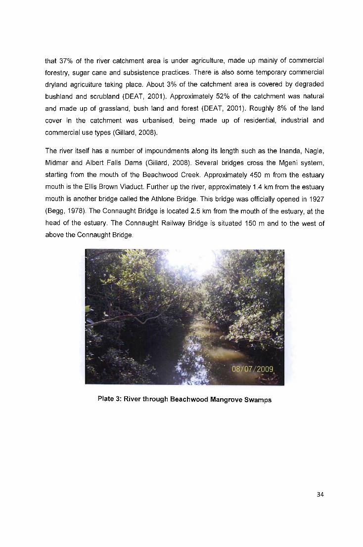
that 37% of the river catchment area is under agriculture, made up mainly of commercial
forestry, sugar cane and subsistence practices. There is also some temporary commercial
dryland agriculture taking place. About 3% of the catchment area is covered by degraded
bushland and scrubland (DEAT, 2001). Approximately 52% of the catchment was natural
and made up of grassland, bush land and forest (DEAT, 2001). Roughly 8% of the land
cover in the catchment was urbanised, being made up of residential , industrial and
commercial use types (Gillard, 2008).
The river itself has a number of impoundments along its length such as the Inanda, Nagle,
Midmar and Albert Falls Dams (Gillard, 2008). Several bridges cross the Mgeni system,
starting from the mouth of the Beachwood Creek. Approximately 450 m from the estuary
mouth is the Ellis Brown Viaduct. Further up the river, approximately 1.4 km from the estuary
mouth is another bridge called the Athlone Bridge. This bridge was officially opened in 1927
(Begg , 1978). The Connaught Bridge is located 2.5 km from the mouth of the estuary, at the
head of the estuary. The Connaught Railway Bridge is situated 150 m and to the west of
above the Connaught Bridge.
Plate 3: River through Beachwood Mangrove Swamps
34

Source: Botes (2009)
Plate 4: Map of Mgeni Estuary and Beachwood Mangrove Swamps
The Mgeni Estuary is a popular recreational zone used for bait collection, angling, water
sports and bird watching. The world famous Duzi Canoe Marathon actually finishes within
the Mgeni Estuary study area. Effluent and storm water is disposed into the Mgeni River and
this works its way down into the estuary. Another recreational area is the Beachwood
Mangrove Nature Reserve that covers approximately 76 hectares to the north of the study
area and has the largest mangrove trees in the entire Durban area (Plate 4). The mangrove
swamps contain several species of mangrove trees such as the pioneering white mangrove
(Laguncularia racemosa) , black mangroves (Avicennia germinans) and the rarer red
mangrove (Rhizophora mangle) (McNae, 1963).
Along the shoreline east of the mangrove swamps, there are sand dunes where creeping
plant species and pioneer bushes and grasses can be found. Further inland from the
swamps are salt marshes, grasslands, thornveld and coastal forest areas (Berjack et al.,
1981). The Beachwood Mangrove Reserve is rich in birdlife and numerous natural trails and
35
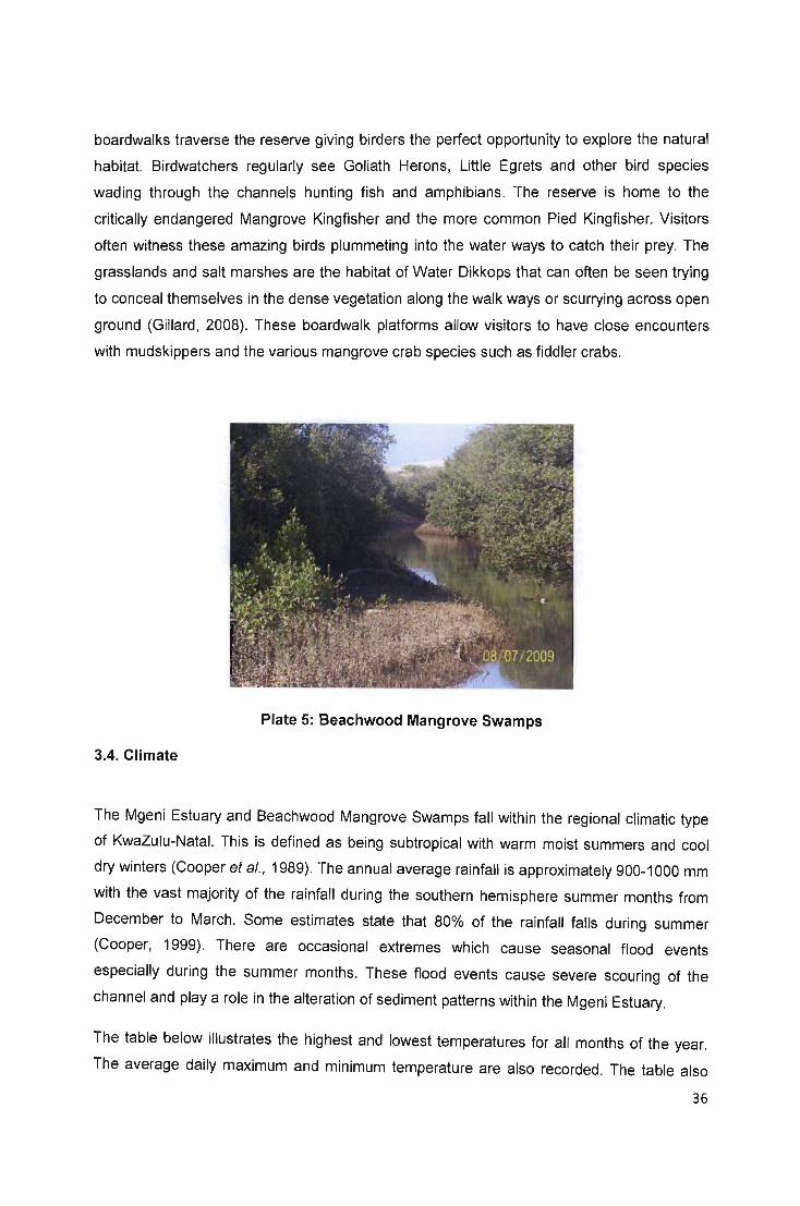
boardwalks traverse the reserve giving birders the perfect opportunity to explore the natural
habitat. Birdwatchers regularly see Goliath Herons, Little Egrets and other bird species
wading through the channels hunting fish and amphibians. The reserve is home to the
critically endangered Mangrove Kingfisher and the more common Pied Kingfisher. Visitors
often witness these amazing birds plummeting into the water ways to catch their prey. The
grasslands and salt marshes are the habitat of Water Dikkops that can often be seen trying
to conceal themselves in the dense vegetation along the walk ways or scurrying across open
ground (Gillard , 2008). These boardwalk platforms allow visitors to have close encounters
with mudskippers and the various mangrove crab species such as fiddler crabs.
Plate 5: Beachwood Mangrove Swamps
3.4. Climate
The Mgeni Estuary and Beachwood Mangrove Swamps fall within the regional climatic type
of KwaZulu-Natal. This is defined as being subtropical with warm moist summers and cool
dry winters (Cooper et al., 1989). The annual average rainfall is approximately 900-1000 mm
with the vast majority of the rainfall during the southern hemisphere summer months from
December to March. Some estimates state that 80% of the rainfall falls during summer
(Cooper, 1999). There are occasional extremes which cause seasonal flood events
especially during the summer months. These flood events cause severe scouring of the
channel and playa role in the alteration of sediment patterns within the Mgeni Estuary.
The table below illustrates the highest and lowest temperatures for all months of the year.
The average daily maximum and minimum temperature are also recorded . The table also
36
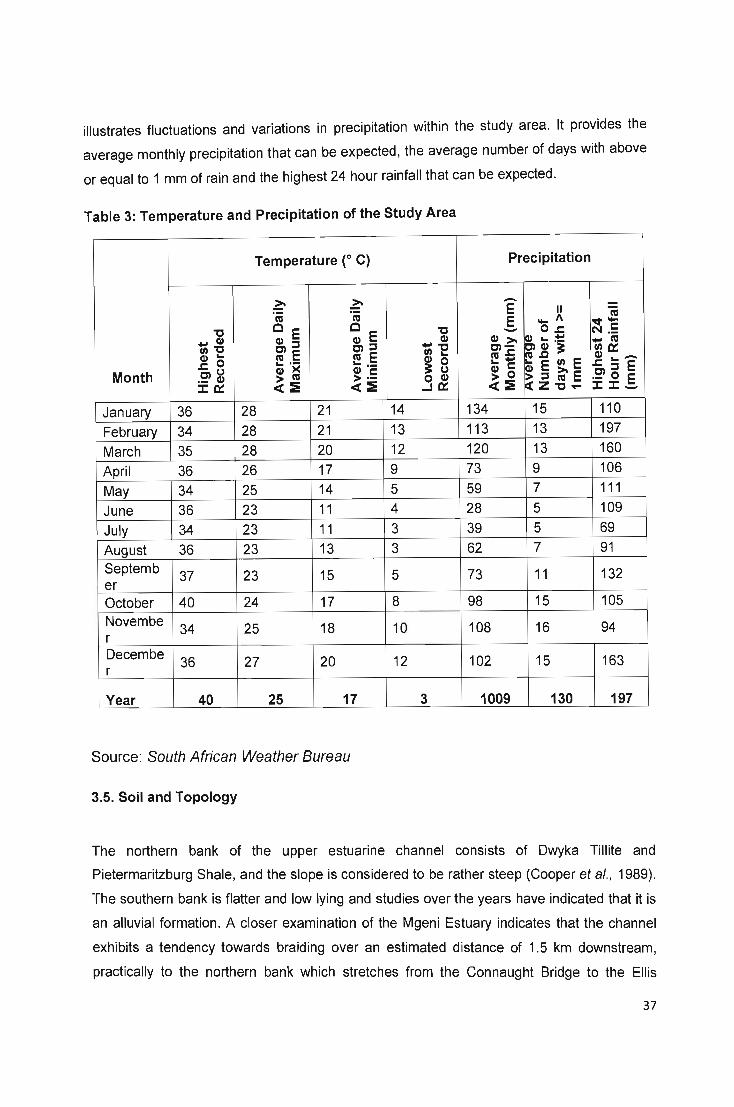
illustrates fluctuations and variations in precipitation within the study area. It provides the
average monthly precipitation that can be expected, the average number of days with above
or equal to 1 mm of rain and the highest 24 hour rainfall that can be expected.
Table 3: Temperature and Precipitation of the Study Area
Temperature (0 C) Precipitation
~ ~ -E II iij .; cu E .... /\ ~ .... '0 C E C
E '0 - OJ: N .5 .... (I) (I) :::I (I) :::I (I) (I) >.
~~l .... cu
III '0 ~E g'e .... '0 CJ)- 1Il~
(I) ... III ... cuJ: (1) ... _
J: 0 .... - ... .- ; 8 ....... E III E J::::IE cnO (I) >< (I) c::: (I) c::: ~ :::I ~ E Month ._ (I) > cu > .- o (I) > 0 .21 0 E
::I:~ «~ «~ ...J~ «~ ... z '0 '"' ::I:::I:_
January 36 28 21 14 134 15 110
February 34 28 21 13 113 13 197
March 35 28 20 12 120 13 160
April 36 26 17 9 73 9 106
May 34 25 14 5 59 7 111
June 36 23 11 4 28 5 109
July 34 23 11 3 39 5 69
August 36 23 13 3 62 7 91 Septemb
37 23 15 er 5 73 11 132
October 40 24 17 8 98 15 105 Novembe r 34 25 18 10 108 16 94
Oecembe 36 27 20 12 102 15 163 r
Year 40 25 17 3 1009 130 197
Source: South African Weather Bureau
3.5. Soil and Topology
The northern bank of the upper estuarine channel consists of Owyka Tillite and
Pietermaritzburg Shale, and the slope is considered to be rather steep (Cooper et al., 1989).
The southern bank is flatter and low lying and studies over the years have indicated that it is
an alluvial formation. A closer examination of the Mgeni Estuary indicates that the channel
exhibits a tendency towards braiding over an estimated distance of 1.5 km downstream,
practically to the northern bank which stretches from the Connaught Bridge to the Ellis
37

Brown Viaduct (Gillard, 2008). Meanwhile, the southern bank has a fairly continuous stream
of flow. A groyne was installed to prevent tidal scouring and this structure has assisted in
stabilizing the southern part of the estuary mouth and managed to control the southward
movement of sand spits or long shore drift (Cooper et a/., 1989). Cooper et a/. (1989) found
that the, "Activity of the wave tides producing long-near-shore drift extending southwards,
constricts the channel outlet causing periodic closure of the channel, hence flooding the
lagoon .. .. . " (Cooper et a/., 1989; 5).
3.S. Sediment
Soil erosion within the Mgeni catchment is significant, and as a result the river carries a
considerable silt load. Studies have shown that an estimated 70 000 tons of silt per year was
carried out into the Indian Ocean between 1958 and 1961 (Begg, 1978). As outlined above,
the construction of the Inanda Dam in the mid 80s has reduced the mean annual discharge
of the Mgeni River by an estimated 4%. This is due to the introduction of the water release
policy which has contributed to the increase in discharge events (Garland and Moleko,
2000). As a result of a controlled outflow, the sediment is being held back behind the dam
wall which has led to a reduction in the sediment flow downstream. However, despite the
fact that sediment within the estuary had not changed significantly since 1989, the sediment
texture has gradual become finer. This study found that sand mining operations in the Mgeni
River would probably cease within the next couple of decades and the estuary would then
probably begin to deepen as the residual pre-dam sediment is washed out into the Indian
Ocean without being replaced by new sedimentary material from upstream (Garland and
Moleko, 2000) . Mgeni sediment is vital for natural beach nourishment, and the cutting off of
this sediment delivery system will have a long term detrimental effect on adjacent beaches
(Garland and Moleko, 2000).
3.7. Area and Extent ofthe Estuary and Mangroves
The total area covered by the Mgeni Estuary and Beachwood is approximately 48 ha on a
spring tide (Begg, 1978). The axial length of the estuary is less than 1. 6 km. However, a
salinity survey which was conducted on the incoming spring tide during 1972 established
that it was in reality approximately 2.5 km. The shoreline length of the estuary is 8.2 km
while Beachwood Mangroves cover around 6 km2• The total shoreline length is 14. 2 km and
the estuary estimated to be 600 m wide near the mouth at the spring tide (Begg , 1978). The
actual entrance to the Beachwood Creek Channel is around 20 m wide as seen in the
38
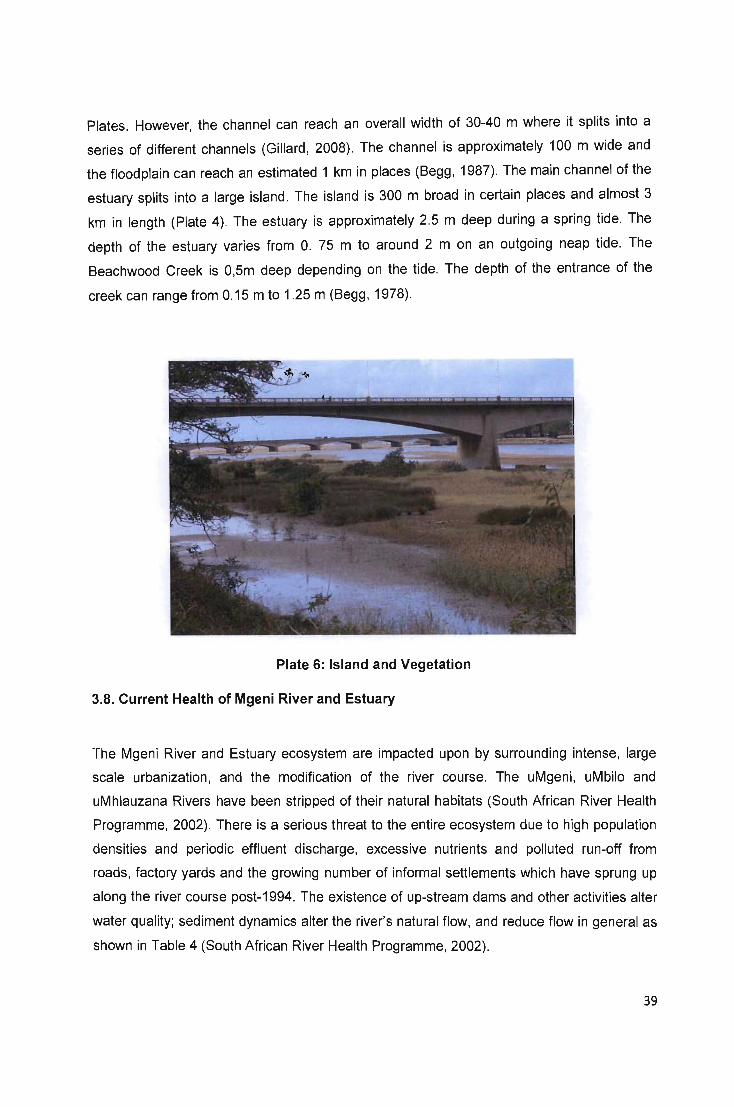
Plates. However, the channel can reach an overall width of 30-40 m where it splits into a
series of different channels (Gillard, 2008). The channel is approximately 100 m wide and
the floodplain can reach an estimated 1 km in places (Begg, 1987). The main channel of the
estuary splits into a large island. The island is 300 m broad in certain places and almost 3
km in length (Plate 4). The estuary is approximately 2.5 m deep during a spring tide. The
depth of the estuary varies from O. 75 m to around 2 m on an outgoing neap tide. The
Beachwood Creek is 0,5m deep depending on the tide. The depth of the entrance of the
creek can range from 0.1 5 m to 1.25 m (Begg , 1978).
Plate 6: Island and Vegetation
3.8. Current Health of Mgeni River and Estuary
The Mgeni River and Estuary ecosystem are impacted upon by surrounding intense, large
scale urbanization , and the modification of the river course. The uMgeni, uMbilo and
uMhlauzana Rivers have been stripped of their natural habitats (South African River Health
Programme, 2002). There is a serious threat to the entire ecosystem due to high population
densities and periodic effluent discharge, excessive nutrients and polluted run-off from
roads, factory yards and the growing number of informal settlements which have sprung up
along the river course post-1994. The existence of up-stream dams and other activities alter
water quality; sediment dynamics alter the river's natural flow, and reduce flow in general as
shown in Table 4 (South African River Health Programme, 2002).
39
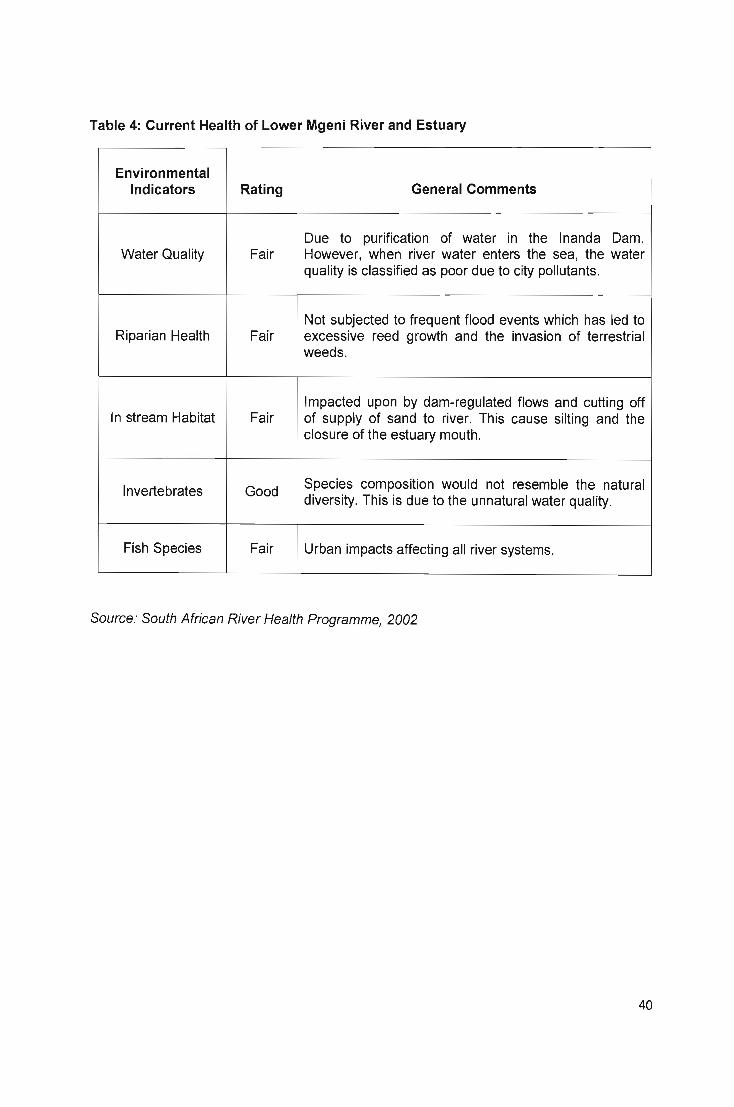
Table 4: Current Health of Lower Mgeni River and Estuary
Environmental Indicators Rating General Comments
Due to purification of water in the Inanda Dam. Water Quality Fair However, when river water enters the sea, the water
quality is classified as poor due to city pollutants.
Not subjected to frequent flood events which has led to Riparian Health Fair excessive reed growth and the invasion of terrestrial
weeds.
Impacted upon by dam-regulated flows and cutting off In stream Habitat Fair of supply of sand to river. This cause silting and the
closure of the estuary mouth.
Invertebrates Good Species composition would not resemble the natural diversity. This is due to the unnatural water quality.
Fish Species Fair Urban impacts affecting all river systems.
Source: South African River Health Programme, 2002
40
Chapter Four
Materials and Methods
4.1. Introduction
This study focuses on establishing whether wetland bird species can be used as
environmental indictors to monitor changes within and surrounding estuarine and mangrove
ecosystems. In order to determine whether wetland birds have the potential to become
meaningful environmental indicators, several objectives must be achieved through a
systematic and rigorous process using various research methods. This will involve the
examination of all available wetland bird census data provided by the Total CWAC Report
Coordinated Water bird Count in South Africa, and the analysis of aerial imagery to identify
land cover changes within and surrounding the study area, from year to year, and to see
whether such changes impacted on wetland bird populations.
4.2. Materials Used in the Study
4.2.1. Data on Wetland Bird Species
4.2.1.1 The Total CWAC Report-Coordinated Waterbird Counts in South Africa
During the course of the study a review of all available bird census data was undertaken.
The Total CWAC Report-Coordinated Waterbird Counts in South Africa is a detailed
publication, produced by the University of Cape Town's Avian Demography Unit, which
summarizes all the results of co-ordinated bird wetland and estuary counts throughout the
whole of Southern Africa (Wheeler, 2008). CWAC counts focus on wetland and estuary
ecosystems and take place biannually, during both winter and summer. Each individual site
is visited and a bird count is undertaken six times within each season. Data collected in the
41

field is subjected to statistical analysis to determine the correlation between two different
variables. Basically these produce a series of trend graphs indicating annual variations in
observed numbers of key species over the period covered (Wheeler, 2008).
The CWAC Report was reviewed, and the historical records of bird sightings in the Mgeni
Estuary and Beachwood Mangrove study area were analysed to determine whether
fluctuations in wetland bird populations over the study period could be correlated with land
cover changes within the same period . If a direct relationship between variations in bird
populations and land cover change could be established within the study period , this would
signify that wetland bird species could be used to effectively monitor land cover change
within and surrounding estuarine and mangrove ecosystems within South Africa.
4.2.1.2. Interviews with Local Ornithological Experts
Direct interaction in the form of unstructured interviews with the ornithologists was essential
to help build trust and develop a working relationship. This research method was used to
confirm the findings uncovered by the analysis of the avian literature material and secure
additional data on wetland bird behaviour and habitat requirements. Conducting interviews is
the most obvious means of gathering essential data 'straight from the horse's mouth'.
4.2.1.3. Archival Aerial Imagery
Aerial imagery is the original form of remote sensing used in topographic mapping and
environmental studies and allows for rapid acquisition of accurate, up-to date information
about the size, location and the character of objects on the surface of the earth (Carver,
1981 ; Campbell, 19983. Aerial remote sensing assists in the completion of maps because of
their concise representation of the patterns found on the ground (Longley et a', 2007).
Vertical aerial imagery is used in the mapping process and will assist in the identification of
land cover changes that occurred within and surrounding the Mgeni Estuary and Beachwood
Mangrove ecosystems over time. Vertical imagery makes it easier to locate and measure the
distance between different objects and features. These measurements can then be
compared against older images to determine changes over time (Mitchel , 1981 , Campbell ,
1983). Secondly, because historical land cover change databases were required for this
study, and relevant aerial imagery of the Mgeni Estuary and Beachwood Mangrove Swamps
was available, it was more cost effective to use these images than undertake field surveys,
although ground truthing was a necessary component of the study (Longley et a', 2007). 42

Because of these advantages, this study obtained vertical aerial imagery of the study area
from the Map Centre CC and from the eThekwini Municipality, who provided a series of
rectified aerial photographs of the study area. Additional images were found in the aerial
photograph archives stored in the University of KwaZulu-Nata/'s Environmental Science
Oepartment campus library on the Westville Campus. Based on the information available, it
was decided to only examine and analyse aerial imagery taken over intervals of five to seven
years. The set of 1991 and 1997 images, provided by the eThekwini Municipality, was
selected along with the rectified 2002 and 2008 images provided by the Map Centre CC.
Table 5 outlines the aerial imagery obtained from the Map Centre CC, eThekwini
Municipality and the library aerial photograph archives of Environmental Science
Oepartment's Westville Campus.
Table 5: Aerial Imagery of the Mgeni Estuary and Beachwood Mangrove Swamps
forming the Basis of this Study
Job Map Year Scale Type Photographs Quantity
Number
Map Centre Contact 2008 1:50000 - - 5
CC Print
Map Centre Contact 2007 1:50000 - - 6
CC Print
eThekwini Contact 2003 1:30000 32 4,8,9 3
Municipality Print
UKZN Lib Contact
1999 1:10000 242 13,14 2 Print
eThekwini Contact 1997 1 :11 000 230 29,30 2
Municipality Print
eThekwini Contact 1991 1:30000 11 140,141 2
Municipality Print
4.2.1.4. Discounted Malerial
As mentioned above, this study focused on the identification and mapping of land cover
class changes within the Mgeni Estuary and Beachwood Mangrove Swamps during the
study period, the analysis and recording of changes in land cover classes over time within
this defined study area, the review and assessment of changes in avian indicator
populations; and finally to determine if there is a Significant relationship between changes in
43

the populations of indicator bird species, and related changes in the patterns of land cover
classes within the estuarine and mangrove swamp study area.
The researcher critically assessed and reviewed various scientific and non-scientific
research methods and approaches that were deemed as potentially beneficial to this study.
However, after examination and consultation with prominent academics, it was decided that
any method considered on the periphery of the study, or not considered necessary for
formulating accurate conclusions relative to study objectives would be discounted or
excluded. Examples would include the measurement of stream flow and the assessment of
river water quality.
4.3. Methods Used in the Study
4.3.1. Evaluating Land Cover Change
4.3.1.1. Land Cover Classification System
After several field visits to the study area and examining the aerial imagery, each land cover
class was identified. The Mgeni Estuary and Beachwood Mangrove Swamps was found to
comprise mainly open water, mudflats, mangrove forest , marsh and coastal forest as shown
in Table 6 below. Satellite and aerial imagery remote sensing techniques have been
developed to provide an effective tool for assessing land cover classification and land use
acquisition (Thompson, 1996).
In most instances the majority of land cover classification schemes have been developed
around the specific user's objectives. As such, these are often influenced by the
geographical location of the study area and the data capabilities that are at the disposal of
that user (Thompson, 1996). As a result, not many land use classification systems are
comparable for directly relevant to the Mgeni Estuary and Beachwood Mangrove Swamp
study area.
A standard hierarchical framework that can be used for the classification of remotely sensed
data has been developed for the South African environment (Thompson, 1996). The
researcher adopted this land classification system as it provided the widest range of
recognised land cover types which could be applied successfully to the Mgeni study area. In
particular, the hierarchal classification for both water bodies and wetlands has been
specifically developed to be broad, because wetland nomenclature and classification
44

schemes are normally formulated and applied to specific mapping or management
requirements. To provide an extensive set of subclasses within this land use classification
fields would be impractical (Thompson, 1996).
However, the researcher developed and applied subclasses within these fields due to the
diversity of land cover types within the Mgeni Estuary and Beachwood Mangrove Swamps.
Secondly, the selected avian indicator species are adapted to foraging , roosting and
breeding within specific habitat types i.e. land cover subclasses. The specific subclasses
developed for this study were based upon a particular classification system used during a
land classification study in Maputaland, South Africa (Lubbe, 1996). The vegetation and soil
types of Maputaland mirror those found within the study area and, therefore, specific land
cover subclasses were selected and adopted for this study.
Table 6: Thompson and Lubbe (1996) Land Cover Classes and Subclasses
Level1 Level 2 Level 3
Forest Coastal Forest I
Forest and Woodland Woodland Island Mangrove Vegetation
Wooded Grassland
Mangrove
Thicket
Thicket, Bushland, Scrub Forest
and High Fynbos Scrub Forest
None Bush Clumps
High Heathland
Scrubland Scrubland and Low Fynbos None
Low Fynbos
45

Grassland Unimproved Grassland Grass Area
Improved Grassland Grassland and Scrub
Lagoon Shallow (Under 0,5 m)
Waterbodies Estuary Open (Between 0,5 and 1,5
m) Lake
Dam
Pan
Stream
River
Reed Beds and Marsh None Wetlands
Reed Beds and Grassland
Residential
Commercial
UrbanI Built Up Area Industrial None
Recreational
Conservation
Beach
Mudflats Other Land Cover Classes
Sandbanks None
Salt Marsh
Sources. Thompson (1996) and Lubbe (1996)
46
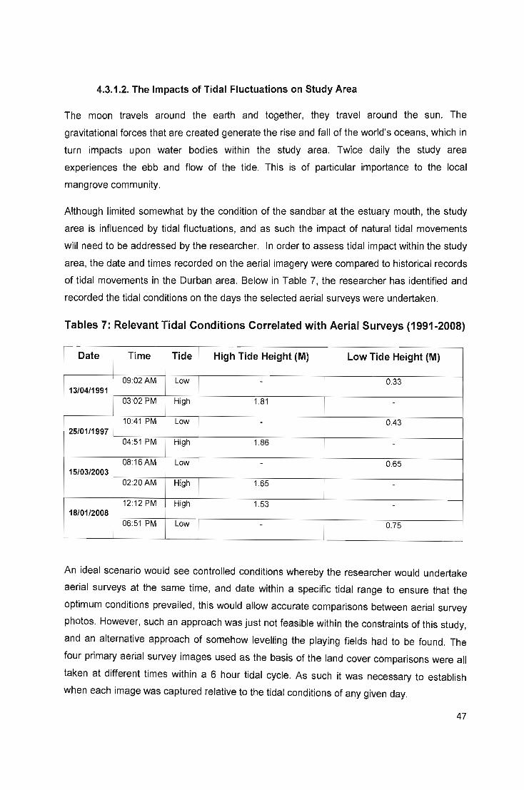
4.3.1.2. The Impacts of Tidal Fluctuations on Study Area
The moon travels around the earth and together, they travel around the sun. The
gravitational forces that are created generate the rise and fall of the world's oceans, which in
turn impacts upon water bodies within the study area. Twice daily the study area
experiences the ebb and flow of the tide. This is of particular importance to the local
mangrove community.
Although limited somewhat by the condition of the sandbar at the estuary mouth, the study
area is influenced by tidal fluctuations, and as such the impact of natural tidal movements
will need to be addressed by the researcher. In order to assess tidal impact within the study
area, the date and times recorded on the aerial imagery were compared to historical records
of tidal movements in the Durban area. Below in Table 7, the researcher has identified and
recorded the tidal conditions on the days the selected aerial surveys were undertaken.
Tables 7: Relevant Tidal Conditions Correlated with Aerial Surveys (1991-2008)
Date Time Tide High Tide Height (M) Low Tide Height (M)
09:02AM Low - 0.33 13/04/1991
03:02 PM High 1.81 -
10:41 PM Low - 0.43 25/01/1997
04:51 PM High 1.86 -
08:16 AM Low - 0.65 15/03/2003
02:20AM High 1.65 -
12:12 PM High 1.53 -18/01/2008
06:51 PM Low - 0.75
An ideal scenario would see controlled conditions whereby the researcher would undertake
aerial surveys at the same time, and date within a specific tidal range to ensure that the
optimum conditions prevailed, this would allow accurate comparisons between aerial survey
photos. However, such an approach was just not feasible within the constraints of this study,
and an alternative approach of somehow levelling the playing fields had to be found . The
four primary aerial survey images used as the basis of the land cover comparisons were all
taken at different times within a 6 hour tidal cycle. As such it was necessary to establish
when each image was captured relative to the tidal conditions of any given day.
47
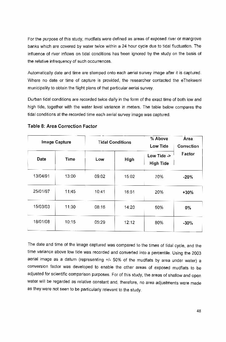
For the purpose of this study, mudflats were defined as areas of exposed river or mangrove
banks which are covered by water twice within a 24 hour cycle due to tidal fluctuation. The
influence of river inflows on tidal conditions has been ignored by the study on the basis of
the relative infrequency of such occurrences.
Automatically date and time are stamped onto each aerial survey image after it is captured.
Where no date or time of capture is provided, the researcher contacted the eThekweni
municipality to obtain the flight plans of that particular aerial survey.
Durban tidal conditions are recorded twice daily in the form of the exact time of both low and
high tide, together with the water level variance in meters. The table below compares the
tidal conditions at the recorded time each aerial survey image was captured .
Table 8: Area Correction Factor
% Above Area Image Capture Tidal Conditions
Low Tide Correction
Low Tide -> Factor
Date Time Low High High Tide
13/04/91 13:00 09:02 15:02 70% -20%
25/01/97 11 :45 10:41 16:51 20% +30%
15/03/03 11 :30 08:16 14:20 50% 0%
18/01/08 10:15 05:29 12:12 80% -30%
The date and time of the image captured was compared to the times of tidal cycle, and the
time variance above low tide was recorded and converted into a percentile. Using the 2003
aerial image as a datum (representing +1- 50% of the mudflats by area under water) a
conversion factor was developed to enable the other areas of exposed mudflats to be
adjusted for scientific comparison purposes. For of this study, the areas of shallow and open
water will be regarded as relative constant and, therefore, no area adjustments were made
as they were not seen to be particularly relevant to the study.
48

Finally, the digitised areas (Ha) of exposed mudflats were then adjusted by the conversion
factor calculated in Table 8 above as outlined in the table below. Whilst not precise, the
above data correction methodology offers a simple method of adjusting a significant land
cover type, tidal fluctuations such that reasonable comparisons can be made between the
various aerial survey images.
Table 9: Corrected Mudflat Area (Ha) Values
Year Digitised Mudflat Corrective Factor Corrected Area
Area (Ha) (%) (Ha)
See Table 8
1991 20.64 -20% 16.51
1997 10.77 +30% 14.00
2003 11.54 00% 11 .54
2008 6.06 -30% 4.24
4.3.1.3. Scanning of Aerial Imagery
Because aerial imagery can be distorted by variations in ground relief, the curvature of the
camera lens or the tilt of the plane, there is the possibility that such imagery might be an
inaccurate representation of the earth's surface (Carver, 1981; Mitchel 1981; Campbell;
1983). The resolution of images might also present as a problem in terms of contrast, colour
and tone of the aerial images.
The first step is to minimise inaccuracies due to distortion and resolution is to scan imagery
into an electronic format. A Hewlett-Packard Scanjet 5370C Scanner was used for this
purpose. Initially, it was felt that the images should be scanned at 400 dpi. However, the
poor resolution of the images in terms of contrast and colour made visually identifying the
differences between land covers difficult during digitizing. To ensure a greater level of
accuracy, it was decided that the images would be rescanned at 1200 dpi to ensure optimal
resolution. This process is referred to as scanning data entry. The process involved the initial
raster scanning for the next step of on-screen digitizing (Davis, 2001). The aerial imagery
was edited once the process was completed. The scanner produces raster files forming the
49

background images for the on-screen digitizing process, or as a raster image to be
combined with remote sensing data obtained for the study (Longley et aI, 2007).
4.3.1.4. Georeferencing
The next step after the scanning of the aerial imagery is referred to as georeferencing. It was
decided that the georeferncing process would be conducted by the Pietermaritzburg-based
company Map Centre CC. The series of scanned images were emailed to the company and
their technicians examined the images and georefernced them. Basically, all GIS data files
have real-world coordinate systems that make them suitable for use as geographic data
(Longley et aI, 2007). This process involved data being fixed to a standard coordinate
system, geographically linking the aerial images of the Mgeni Estuary or Beachwood
Mangrove Swamp, to the earth.
After rigorous examination of the images, four separate points or reference features were
identified in each aerial image. Field surveys were conducted within the study area and the
GPS coordinates of these points/features were recorded using a portable GPS device. All
real world coordinate positions of key features found within all the aerial photographs were
collected during these field surveys. The features or points selected included bridges,
buildings and road intersections. This data will then be incorporated into Microsoft's Excel
spreadsheet to assist in merging field attributes with GPS data.
4.3.1 .5. On-Screen Digitizing
The digitizing process is completed on a computer monitor. The scanned aerial images of
the study area are displayed on the desktop computer screen and the features that are
displayed are traced using a mouse. The latest aerial images would be digitized first. A
feature type is selected by the tracer as a point, line or polygon. These features are then
traced by the mouse in a similar fashion to the puck on a digitizing table. The GIS data files
are specific to either point, line or polygon features. Each different type will be digitized
separately by the tracer during the digitizing process.
The digitizing process is organised to ensure that features of all types within the images are
digitized and their locations are noted. Every feature within the database is then classified
and each receives a label system assigned before the digitizing process begins (Longley et
aI, 2007). Magnification and the moving view are basic functions that require a few clicks on
the mouse buttons on the screen to allow the tracer to zoom into aerial images to help
ensure that greater accuracy is achieved while tracing features.
so

The aerial imagery obtained from the university library was not 'rectified'. This means that
these images were not corrected to a georeferenced location, and were nothing more than
'uncorrected' pictures that could not be used (Davis, 2001). In order to correct this fault, the
tracer used an option that splits the computer screen with the georeferenced aerial
photographs on one side, and the unreferenced aerial photographs are on the other. The
features and points that are displayed on the screen are related by coordinates.
The next step is to select thirty-two common points on the images, each represented by a
coloured dot that is positioned at each of these chosen locations. The aerial photographs are
adjusted using the affine transformation program which basically stretches and deforms the
aerial images according to these identified coordinate points (Davis , 2001). This program
transforms the digitizer table coordinates to real-world coordinates for the digitized aerial
photographs, using all the reference points and projection information that is available
(Davis, 2001).
4.3.1.6. Projecting Land Cover Maps
Map projections are the representation of the spherical earth onto a piece of paper as a
map, or a digital image on a computer monitor. To assess changes in land cover patterns
within the study area and to facilitate the comparison between different years, all images had
to have the same map projection (Longley et at, 2007). Therefore, it was essential to select
the ideal map projection required to assess the land cover change patterns, in terms of area
covered, in the Mgeni Estuary and Beachwood Mangrove Swamps.
It is vital that from the beginning of this process that there needs to be an understanding of
the map projection and coordinate system that is required . The coordinate system that will
be adopted is largely determined by eth extent of the area that will be covered during the
study. There are two types of coordinate systems that are applicable for working in 20 data:
Projected and Geographic Coordinate Systems (Longley et at, 2007).
Projected Coordinate systems are ideal for working over a small study areas. The Gauss
Conform Projected Coordinate System that is used in South Africa is simply a Transverse
Mercator Map that has been turned upside down and limited to an area of approximately 2 0
of longitude. This means that it will not extend beyond 10 on either side of the Central
Meridian (Longley et all 2007). This system is often referred to as LO or Longitude Zero
which is based on the Cape Datum. The central meridians are denoted to the LO, followed
by the number of line of longitude. The City of Durban falls within the Map Zone where the
central meridian is denoted as L031 . The datum that has been adopted by South Africa
51

since 1999 is known as the Hartesbeehoek94 (Hart94) which has been based on WGS84 for
a global ellipsoid (Botes, 2009). Therefore, all central meridians are being preceded with
WG. Therefore, the Map Zone in which the City of Durban is found has its central meridian is
denoted as WG31 .
As the study area covers a small portion of the Durban area, it was essential to define the
spatial reference system used in South Africa with the parameters of the Map Zone in which
the Durban is found (Botes, 2009). Therefore, is defined as WG31.
4.3.1.7. Assessing Changes in Land Cover
The mapping of the land cover of the Mgeni Estuary and Beachwood Mangrove Swamps
was completed. The total area of each land cover class was calculated by using the
summary function of ArcMap. The land cover class's attribute table is opened and the field
titled area is selected. The 'Calculate Values' option is clicked and this generates a summary
table which is exported to Microsoft Excel 2007 to be analysed in order to quantify the land
cover changes over the study period.
4. 3.1.8. Positional Error
The National Map Accuracy Standard prescribes positional errors that are allowed to occur
within a database (Longley et a/., 2007). The 1947 US National Map Accuracy Standard
indicates that 95% of all errors should fall below 1/30 inches (Approximately 0.85mm) for all
maps that are of a scale 1: 20 000. While 1/50 inch (0.51 mm) would be acceptable for all
other maps (Longley et a/., 2007). However, it is advisable that positions that are measured
on a map should be subjected to errors of up to 0.5mm at the scale of the map in question.
The researcher applied this approach during the cause of this study.
Table 10: below represents the distance on the ground that corresponds with
O.Smm for the common map scale.
Map Scale Ground distance corresponding to
O.Smm map distance
1 :10 000 5m
1:24 000 12 m
1:50 000 25m
Source. Longley et a/. , 2007
52

4.4. Identification of Avian Indicators
4.4.1. Identification of Wetland Bird Species
Several bird species that utilise the Mgeni Estuary and Beachwood Mangrove ecosystems
for roosting , feeding and breeding were identified during field visits. This identification
process was undertaken by analyzing South African Avian literature such as Roberts Birds
of Southern Africa VII, SAGS Checklist of Southern African Birds and The Important Bird
Areas of Southern Africa (Allen, 2008).
4.4.2. Identification of Indicator Species
Reviewing the avian literature proved valuable as it assisted in the establishment of criteria
to identify twelve bird species that would be used as 'indicator species' for both estuarine
and mangrove habitats. The indicator species were selected based upon their preferred
natural habitats within an estuarine or mangrove ecosystem as evidenced by their foraging
behaviour, dietary requirements, roosting and reproductive requirements noted after
discussions with ornithological experts and the review of available avian literature.
Reviewing the avian literature proved valuable as it assisted in the establishment of criteria
to identify twelve bird species that would be used as 'indicator species' for both estuarine
and mangrove habitats. The indicator species were selected based upon their preferred
natural habitats within an estuarine or mangrove ecosystem as evidenced by their foraging
behaviour, dietary requirements, roosting and reproductive requirements noted after
discussions with ornithological experts and the review of available avian literature. All
available data relating to the fluctuation in the populations of these selected indicator species
was examined to ensure that the data spanned a time scale of two decades. Table 11 lists
all seventeen avian indicator species selected for this study.
53
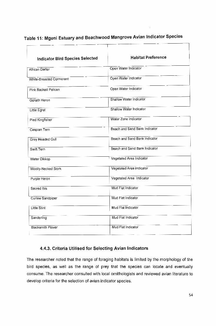
Table 11: Mgeni Estuary and Beachwood Mangrove Avian Indicator Species
Indicator Bird Species Selected Habitat Preference
African Darter Open Water Indicator
White-Breasted Cormorant Open Water Indicator
Pink Backed Pelican Open Water Indicator
Goliath Heron Shallow Water Indicator
Little Egret Shallow Water Indicator
Pied Kingfisher Water Zone Indicator
Caspian Tern Beach and Sand Bank Indicator
Grey Headed Gull Beach and Sand Bank Indicator
Swift Tern Beach and Sand Bank Indicator
Water Dikkop Vegetated Area Indicator
Woolly-Necked Stork Vegetated Area Indicator
Purple Heron Vegetated Area Indicator
Sacred Ibis Mud Flat Indicator
Curlew Sandpiper Mud Flat Indicator
Little Sti nt Mud Flat Indicator
Sanderling Mud Flat Indicator
Blacksmith Plover Mud Flat Indicator
4.4.3. Criteria Utilised for Selecting Avian Indicators
The researcher noted that the range of foraging habitats is limited by the morphology of the
bird species, as well as the range of prey that the species can locate and eventually
consume. The researcher consulted with local ornithologists and reviewed avian literature to
develop criteria for the selection of avian indicator species.
54

For example, Mudflat Zone Indicators (wading wetland avian species) such as the Little
Stint, Curlew Sandpiper, Sanderling and Blacksmith Plover prey on a variety of aquatic
invertebrates found close to the surface of inter-tribal mudflats (Velasquez and Hockey,
1992). Invertebrates such as snails, worms and crabs are visually identified by the bird as
they move across exposed mudflats, and then they are caught, disabled and consumed by
pecking or shallow probing with the bird's beak (Allen, 2008). Some wading bird species
locate their prey by other clues such as surface casts of poychaetete worms, or the
movement of prawns and shrimps as they attempt to irrigate their burrows. These facts
indicate that these wetland bird species have the potential to become avian indicator species
for monitoring changes in the exposed mudflat land cover class.
A summary of the specific habitats, diets, roosting and breeding requirements of the selected
avian indicators was compiled after interviews with local ornithologists and examination of
literature sources is provided in the Appendix F and J, found in the Appendix section .
4.4.4. Analyzing the CWAC Bird Census Data
The Total CWAC Report-Coordinated Waterbird Counts provided a wealth of historical data
relating to the number of wetland birds visiting the Mgeni Estuary and Beachwood Mangrove
ecosystems over the last two decades. The researcher captured and analysed only wetland
bird census data relevant to the selected avian indicator species. This census data was
transferred into Microsoft Office Excel 2007 for easy storage and processing. A series of
trend graphs were generated illustrating the fluctuations in populations of avian indicator
species within the study area over the chosen period of study. Table 13 is an example of the
Total CWAC Report-Coordinated Waterbird Counts.
Table 12: Example of CWAC Avian Census Data
Avian
Indicator
Species Jan-93 Jul-93 Jan-94 Jul-94 Jan-95 Jul-95 Jan-96 Jul-96
PB Pelican 0 0 2 17 3 20 0 2
WB Cormorant 6 44 0 0 10 3 11 54
African Darter 0 4 0 0 4 4 1 37
GH Gull 963 2 548 31 30 54 282 6
Caspian 1 4 1 2 1 5 2 1
Swift Tern 77 16 52 111 46 107 110 68
55
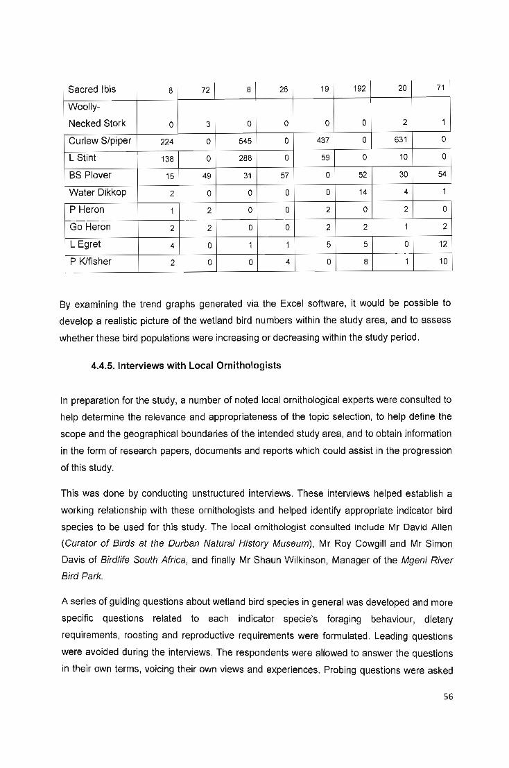
Sacred Ibis 8 72 8 26 19 192 20 71
Woolly-
Necked Stork 0 3 0 0 0 0 2 1
Curlew S/piper 224 0 545 0 437 0 631 0
L Stint 138 0 288 0 59 0 10 0
BS Plover 15 49 31 57 0 52 30 54
Water Dikkop 2 0 0 0 0 14 4 1
P Heron 1 2 0 0 2 0 2 0
Go Heron 2 2 0 0 2 2 1 2
L Egret 4 0 1 1 5 5 0 12
P Klfisher 2 0 0 4 0 8 1 10
By examining the trend graphs generated via the Excel software, it would be possible to
develop a realistic picture of the wetland bird numbers within the study area, and to assess
whether these bird populations were increasing or decreasing within the study period.
4.4.5. Interviews with Local Ornithologists
In preparation for the study, a number of noted local ornithological experts were consulted to
help determine the relevance and appropriateness of the topic selection, to help define the
scope and the geographical boundaries of the intended study area, and to obtain information
in the form of research papers, documents and reports which could assist in the progression
of this study.
This was done by conducting unstructured interviews. These interviews helped establish a
working relationship with these ornithologists and helped identify appropriate indicator bird
species to be used for this study. The local ornithologist consulted include Mr David Allen
(Curator of Birds at the Durban Natural History Museum) , Mr Roy Cowgill and Mr Simon
Davis of Birdlife South Africa, and finally Mr Shaun Wilkinson, Manager of the Mgeni River
Bird Park.
A series of guiding questions about wetland bird species in general was developed and more
specific questions related to each indicator specie's foraging behaviour, dietary
requirements, roosting and reproductive requirements were formulated. Leading questions
were avoided during the interviews. The respondents were allowed to answer the questions
in their own terms, voicing their own views and experiences. Probing questions were asked
56
to try and go beyond the expected answers given by the respondents to obtain a better
understanding of their assumptions.
These interviews helped the researcher to establish an in-depth insight and understanding of
wetland bird species and their behaviour patterns, changes in land use/ cover within the
study area, and other essential information that went beyond the mere "answers". This is an
ideal means of exploring and investigating a topic very broadly. These questions were
specific to the particular ornithologist being interviewed, and the interviews had no formal
structure or protocol. All responses were recorded by writing them down and/or by means of
a Dictaphone, to ensure that data crucial to the study was not lost. The recorded responses
were analysed and collated after the completion of interviews.
4.4.6. Field Survey of current status of Mgeni Estuary and Beachwood
Mangrove Swamps
A series of field surveys were conducted within the Mgeni Estuary and Beachwood
Mangrove Swamp ecosystems to determine precisely where each habitat was located within
the ecosystems, and to generate adequate additional data to test the quality and accuracy of
the aerial image classification process undertaken at desktop level. The field surveys were
carefully planned to give due consideration to the objectives of the study, and the nature of
habitats being surveyed. Most importantly, the field surveys had to coincide with both high
and low tide regimes of the Mgeni Estuary.
Before undertaking a field survey, a basic understanding of the concept of remote sensing is
essential. Remote sensing is a mapping approach that does not require field surveys, and is
often referred to as a 'desk top study'. The aerial imagery obtained from the Map Centre CC
eThekwini Municipality and the library aerial photograph archives from the Environmental
Science Department's Westville Campus, provided the opportunity to distinguish between
different features and habitats within the Mgeni Estuary and Beachwood Mangrove Swamps
according to colour, contrast, pattern, texture and context. The examination of the aerial
imagery was made easier by the high quality of the images. This allowed the boundaries of
the different habitats to be readily indentified and defined. This assisted the series of field
surveys by identifying key features that required physical verification and examination on the
ground.
57

4.5. Assessing the Relationship between Counts of Wetland Bird Indicators and Changes in Land Cover
The overall aim of the study was to determine whether wetland bird species could act as
effective environmental indicators of undesirable change in land use and cover within and
surrounding estuaries and mangrove swamps ecosystems in Southern Africa. In order to
assess the relationship between wetland bird populations and land cover change, a
systematic process was adopted.
A systematic process of identifying and proving a link between the fluctuations in the
populations of indicator bird species, and related changes in land cover, would involve
analyzing and identifying a common trend between the data processed when reviewing the
CWAC Report, and the decline or increase in the total area of each land cover class. In
order to establish the existence of relationships between different variables a process of
statistical analysis was implemented.
4.5.1. Statistical Analysis and the Correlation Coefficient
The researcher undertook a statistical analysis to determine if there was a relationship
between the values provided by the CWAC Wetland Avian Census data for the avian
indicator species and the number of hectares covered by particular land cover classes
identified within the study area that these species rely upon for foraging, roosting and
reproduction within the Mgeni Estuary and Beachwood Mangrove Swamp study area. The
most appropriate means of establishing if there was indeed a relationship between two
variables of interest and how closely the two variables change in relationship to each other,
is the application of a correlation coefficient and linear regression (Hogg and Craig, 1975).
In simple regression the coefficient of determination, R2 is the square of the correlation
coefficient, and 0 :::; R 2:::; 1. An R 2 value close to 1 indicates a strong linear relationship
(Hogg and Craig, 1975). Consider the variables (x,y) with data points (x1, y1}, ... m (xn,yn) .
The sample correlation coefficient is defined as:
58
The correlation coefficient is a statistical measure which determines the strength of the linear
relationship. The two variables that are compared against each other are known as the
independent and dependent variables (Hogg and Craig, 1975). The independent variable is
the variable that changes which is beyond human control. In the case of this study, time is
the independent variable because it goes on whether the researcher would like it or not.
Basically, in a very simple sense, time always increases and will never decrease (Hogg and
Craig, 1975).
The dependent variable changes as a result of the changes taking place in the independent
variable (Hogg and Craig, 1975). For example, the dependent variables in this study are the
number of avian indicators recorded and the areas covered by the land cover classes and
subclasses within the study area. Therefore, the number of birds recorded and the area
covered by a specific land cover class or sub-class within the study area depends on the
amount of time that passes.
For the purposes of this study it was essential to find a mathematical device to determine the
amount by which these variables correlated with each other. A correlation coefficient can
take on values between -1 and 1. A correlation coefficient of 0 means that changes in the
independent and dependent variable appear to be random and completely unrelated to each
other (Hogg and Craig, 1975). In other words there is no relationship between the variables
and thus there is no linear correlation . A correlation coefficient of +1 basically indicates that
the two variables are perfectly correlated with each other and as the independent variable
increases or decreases it will be accompanied by the exact increases or decreases in the
dependent variable. A correlation coefficient of +0.75 indicates that a change in the
independent variable should result in a comparable increase in the dependent variable
(Hogg and Craig, 1975).
If there is a negative correlation coefficient like -0.6508 this means that the two variables will
respond in opposite directions. While the one increases, the other variable will decrease. It is
important to note that any correlation coefficients between .00 and .30 should be considered
weak, while those between .30 and.70 are taken as been moderate and any coefficients
between .70 and 1.00 are to be considered high (Hogg and Craig, 1975).
59

Acquisition of aerial imagery for the years 1991, 1997, Acquisition of aerial imagery for the years 1991 and 1997
2003 and 2008 from eThekweni Municipality. from UKZN Environmental Sciences Library.
Scanning of aerial imagery at 1200 dpi to ensure optimal resolution in the form of Tiff
Acquisition of CWAC Image.
Wetland Bird Census ~ Data from University
of Cape Town, Avian Georectification and mosaicking of
Demographic Unit. scanned imagery.
Field visits to identify
Interpretation of aerial imagery . ~ the land cover • classes in study
Identification of twelve area. wetland avian indicator species. On-Screen digitizing of land cover classes,
Allocate species to sub-classes and land cover changes within
each land cover study area.
classes and sub-classes with assistance of ornithologists. Editing and projecting land cover maps.
Analysing fluctuations in wetland avian
Additions of attributes of land indicator populations
cover
between 1993 and classes.
2008.
~ Generation of areal statistics
Generation of wetland avian indicator population statistics. Quantifying Change
The researcher undertook statistical analysis to determine if there was a relationship between the fluctuations in selected avian indictor populations and changes in area coverage of land cover classes and sub-classes.
Identification of a possible link between fluctuations in wetland avian indicator populations and changes in land cover within the study area.
Figure 1: Summary of the Steps Followed to Develop the Historical Avian Indicator Changes, Land Cover Change Database and Maps
60
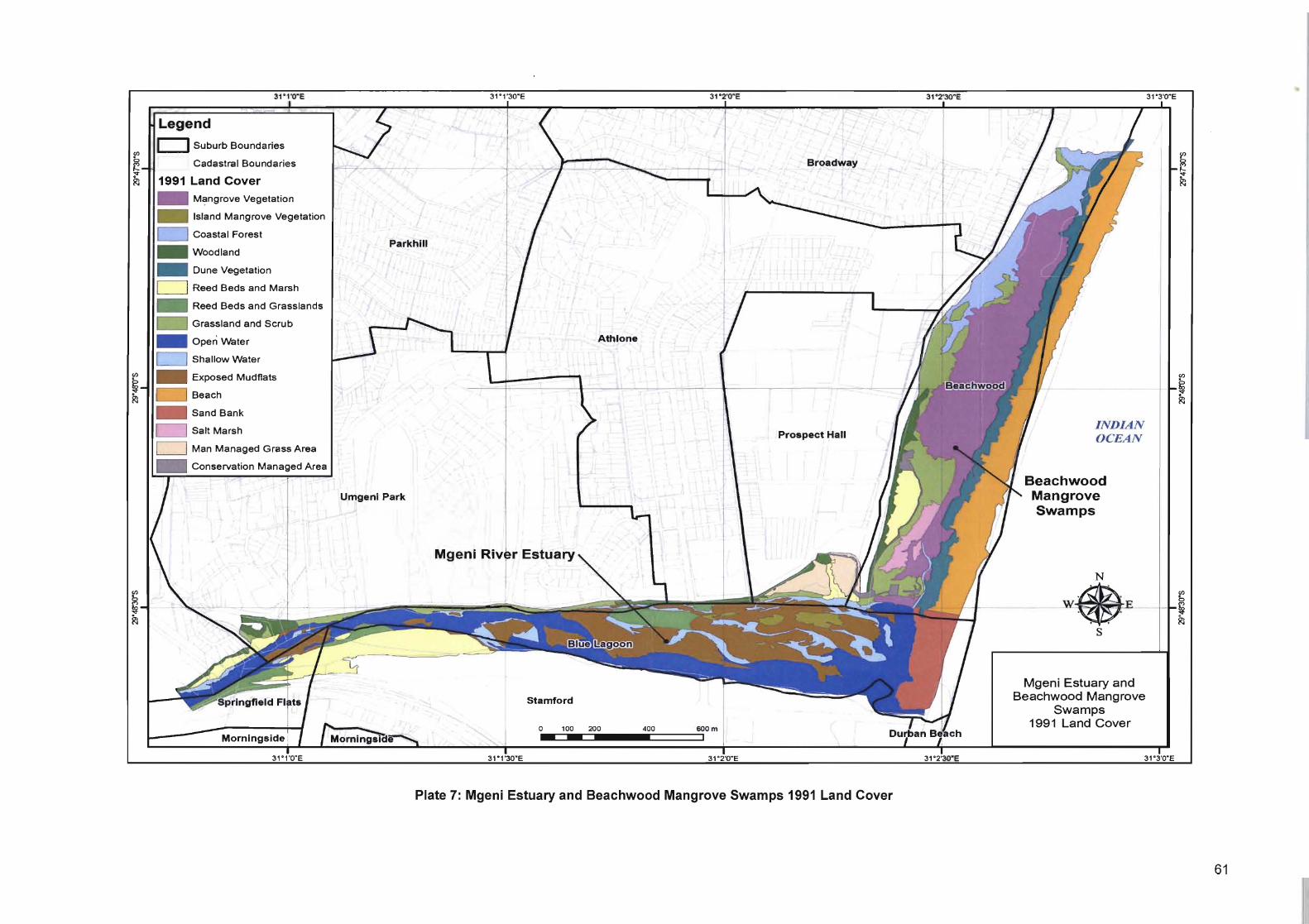
Legend
Cadastral Boundaries
1991 Land Cover _ M~ngrove Vegetation
_ Island Mangrove Vegetation
CJ Coastal Forest
_ woodland
_ Dune Vegetation
CJ Reed Beds and Marsh
_ Reed Beds and Grasslands
Beach
_ SandBank
c=J Salt Marsh
CJ Man Managed Grass Area
1 I Parkhill
Athlone
Prospect Hall
Umgenl Park
Mgeni
Stamford
o 100 200 400 600m
Plate 7: Mgeni Estuary and Beachwood Mangrove Swamps 1991 Land Cover
INDIAN OCEAN
Beachwood Mangrove Swamps
N
s
Mgeni Estuary and Beachwood Mangrove
Swamps 1991 Land Cover
61
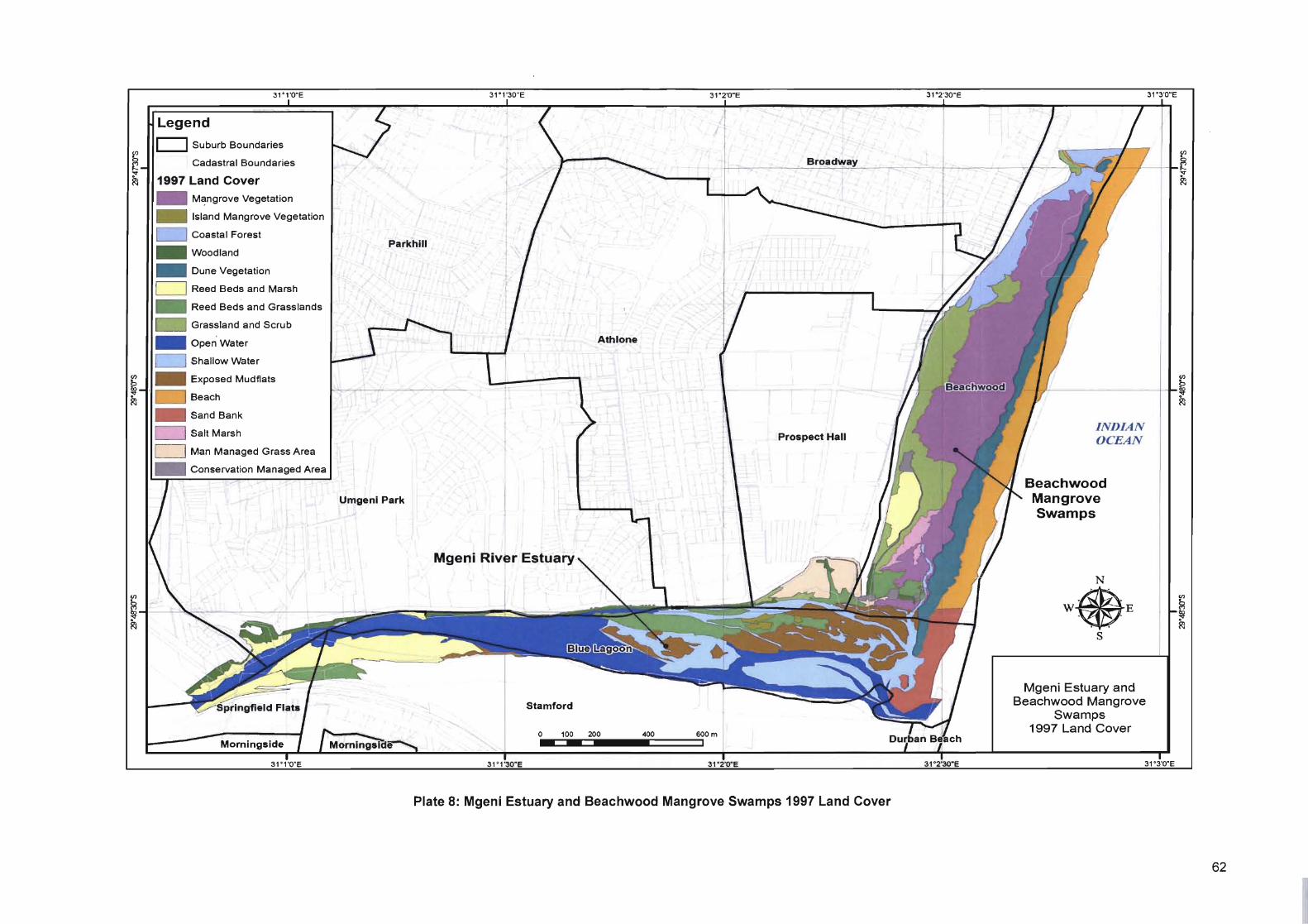
Legend
[::J Suburb Boundaries
Cadastral Boundaries
1997 Land Cover _ M~ngrove Vegetation
_ Island Mangrove Vegetation
L=:J Coastal Forest
_ Woodland
_ Dune Vegetation
c=J Reed Beds and Marsh
_ Reed Beds and Grasslands
Grassland and Scrub
_ Open' Water
L=:J Shallow Water
_ Exposed Mudflats
Beach
_ SandBank
L=:J Salt Marsh
c=J Man Managed Grass Area
_ Conservation Managed Area
I Parkhill
Umgenl Park
Mgeni River Estuary I
Stamford
Athlone
O"cj100 .. ~20.0 ...... ~-=O======~5om
Prospect Hall
Plate 8: Mgeni Estuary and Beachwood Mangrove Swamps 1997 Land Cover
INDIAN OCEAN
Beachwood Mangrove Swamps
N
• ' . . W E . .
s
Mgeni Estuary and Beachwood Mangrove
Swamps 1997 Land Cover
62

31
Legend
c::::J Suburb Boundaries
Cadastral Boundaries
2003 Land Cover _ Mangrove Vegetation
_ Island Mangrove Vegetation
CJ Coastal Forest
_ Woodland
_ Dune Vegetation
CJ Reed Beds and Marsh
_ Reed Beds and Grasslands
Beach
_ SandBank
CJ Salt Marsh
CJ Man Managed Grass Area
_ Conservation Managed Area
, I
Broadway , ............ "r-!-;
"l / Parkhill
Athlone
r"~" .>.. ...... »,. .......
Prospect Hall
Umgeni Park
Mgeni
Stamford
o 100 200 400 - -Plate 9: Mgeni Estuary and Beachwood Mangrove Swamps 2003 Land Cover
31
INDIAN OCEAN
Beachwood Mangrove Swamps
N
s
Mgeni Estuary and Beachwood Mangrove
Swamps 2003 Land Cover
63
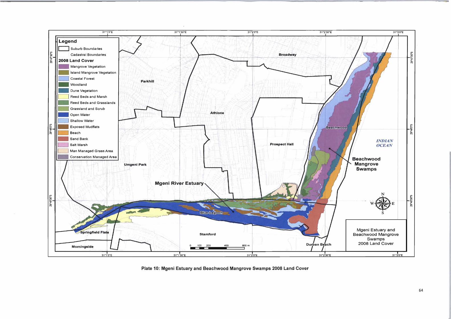
Legend
L::J Suburb Boundaries
Cadastral Boundaries
2008 Land Cover _ Mangrove Vegetation
_ 'Island Mangrove Vegetation
c=J Coast~1 Forest
_ Woodland
_ Dune Vegetation
c=J Reed Beds and Marsh
_ Reed Beds and Grasslands
Grassland and Scrub
C:=J Man Managed Grass Area
_ Conservation Managed Area , j
Morningside i
Parkhill
Umgeni Park
"'"
'/
Athlone
Stamford
o 100 200 400 600 m - -
Prospect Hall
Plate 10: Mgeni Estuary and Beachwood Mangrove Swamps 2008 Land Cover
INDIAN OCEAN
Beachwood Mangrove Swamps
N
W~E ~
s
Mgeni Estuary and Beachwood Mangrove
Swamps 2008 Land Cover
64
Results and Discussion
5.1. Categorization and Mapping of Changes in Land Cover within the Study Area
Categorizing and mapping different land cover types within the Mgeni Estuary and
Beachwood Mangrove Swamps is an essential component of this study. This process would
provide an oppgrtunity to assess whether land cover and related habitats have changed over
time, and consequently whether such changes have impacted on wetland bird populations.
Land cover change detected within an estuary or mangrove swamp should be cause for
concern because of the ecological sensitivity of such ecosystems. Such change could be the
result of for example, fuel wood collection , and water pollution or over utilization of these
ecosystems for recreational purposes. Table 14 illustrates the current land cover types found
within the study area.
5.2. Land Cover Change within the Study Area
Using aerial survey imagery, it was possible to document and map the different land cover
types within the study area. Below the Inanda Dam, the Mgeni River has been extensively
modified, with riparian vegetation and the direction of flow having been drastically altered
opposite the Springfield Industrial Park to accommodate industrial and commercial activities,
and extensive human settlement along the river course, and in the immediate vicinity of the
study area. As a consequence of upstream alterations and modifications to the Mgeni River
course, land cover within the study area has steadily changed in terms of land cover area
(%) as represented in Table 14 below.
This study had to consider the impact of natural tidal movements within the Mgeni Estuary
and Beachwood Mangrove ecosystems. Although limited somewhat by the condition of the
sandbar at the estuary mouth, the study area is influenced by the tidal fluctuation. The rise
and fall of the tides lead to the submersion and eventual exposure of mudflats, sand banks
by fluctuations in water levels.
65

Table 13: Land Cover Changes (1991-2008)
Year
1991 1997 2003 2008
Land Cover Total % of Total %of Total %of Total % of
Area Study Area Study Area Study Area Study
(ha) Area (ha) Area (ha) Area (ha) Area
Beach 18.67 11 .6 16.38 10.2 13.04 8.1 11 .23 6.9
Coastal Forest 7.12 4.5 5.69 3.5 14.07 8.8 18.06 11.2
Conservation 1.13 0.7 0.92 0.6 1.36 0.8 1.39 0.9
Managed Area
Dune Vegetation 9.43 6.0 10.46 6.5 12.60 7.9 7.78 4.8
Exposed Mudflats 16.51 12.8 14.00 6.6 11 .54 7.2 4.25 3.8
Man-Managed Grass 3.07 2.0 3.65 2.3 3.30 2.1 2.95 1.8
Area
Grassland and Scrub 13.21 8.2 11 .51 7.1 3.47 2.2 3.52 2.2
Island Mangrove 1.38 2.0 0.52 0.3 1.53 1.0 3.17 1.9
Vegetation
Mangrove Vegetation 24.85 15.4 28.05 17.4 27.82 17.4 29.81 18.4
Open Water 26.00 16.2 25.69 16.0 19.75 12.3 25.99 16.1
Reed Beds and 4.51 2.8 8.38 5.2 6.79 4.2 9.7 6.0
Grasslands
Reed Beds and 11.64 7.2 12.38 7.7 10.43 6.5 9.6 5.9 Marsh
Salt Marsh 1.85 1.1 1.27 0.7 0.68 0.4 0.95 0.5
Sand Bank 5.46 3.4 4.42 2.7 4.29 2.7 8.75 5.4
Shallow Water 7.28 4.5 16.81 10.4 18.49 11 .6 8.03 5.4
Woodland 4.69 2.9 4.19 2.6 10.91 6.8 8.87 5.5
Total 160.96 100 161.11 100 160.07 100 154.05 100
66

5.3. Tidal Fluctuations and the Impact on Water Bodies, Sand Banks and Exposed Mudflats
Closer examination of the aerial survey imagery has revealed the gradual decline of exposed
mudflats, deep and medium depth water bodies and the increase in shallow water bodies
within the estuarine and mangrove ecosystems. However, these initial assumptions based
on observations, digitization and the calculation of the area covered by exposed mudflats
from a series of aerial images could be misleading . Aerial images are simply a 'snap shot' in
time. They cannot be considered a true reflection of the actual land cover classes occurring
within dynamic ecosystems such as an estuaries or mangrove swamps subjected to tidal
fl uctuations.
Coastal areas experience two daily high (and two low) tides, and the Mgeni Estuary and
Beachwood Mangrove Swamp are therefore affected by such tidal fluctuations . The rise and
fall of the tides leads to dramatic changes in specific land cover within the study area within
a matter of hours, and sometimes minutes. The submerging and exposure of mudflats and
fluctuating water levels make it difficult to establish the true extent of the total area coverage
of various land cover classes.
However, examination of historical tidal archives provided online by Mobile Geographic's
LL T for the eThekwini area, provided a substantial amount of data about low and high tide
events. In order to establish whether an aerial image was captured during a high or low tide
event, the researcher examined the aerial images and contacted the eThekwini Municipality
for the missing times and dates of aerial images to establish the exact time and date of each
image capture.
After comparing the data provided by the tidal archives, and the dates and times of the
flights over the study area, it was discovered that all aerial imagery utilised during the cause
of this study was captured during a transition from low tide to high tide. Therefore, this
provided the researcher with some degree of confidence to continue the land cover change
assessment for water bodies and exposed mudflats.
67

5.4. Open and Shallow Water Bodies Land Cover Sub-Classes
The Mgeni Estuary and Beachwood Mangrove Swamps cover an area of 161 ha. Water
bodies (open and shallow water bodies) are some of the dominant land cover types within
these ecosystems. The water bodies land cover class are broken into two sub-classes. The
first is Open Water and the other Shallow Water. Figure A 1 in the Appendix A displays the
fluctuations in the area covered by Shallow and Open water bodies since 1991.
Table 14: A Summary Table of Area Coverage of Water Land Cover in Mgeni Estuary and Beachwood Mangrove Swamp Study Area
Aerial Image 1991 Aerial Image 1997 Aerial Image 2003 Aerial Image 2008
Land Cover Type % of % of % of % of
Hectares Study Hectares Study Hectares Study Hectares Study Area Area Area Area
Open Water 26.00 16.1 25.69 15.9 19.75 12.3 25.99 16.1
Shallow 7.28 4.5 16.81 10.4 18.49 11.5 8.63 5.4 Water
Open water zones occupied 26.00 ha (16.1 %) of the Mgeni Estuary and Beachwood
Mangrove Study Area in 1991 (Table 14). The open water zone areas decreased gradually
to 25.69 ha (15.9%) cover by 1997. In 2003, deep and medium deep water zones covered
approximately 19.75 ha (12.3%) of the study area. Currently, this land cover type covers
25.99 ha (16.1 %) of the study area. These areas, previously designated as open water
zones, have steadily reverted to significantly shallower zones as evident from aerial imagery.
Plate 11: Open Water
68
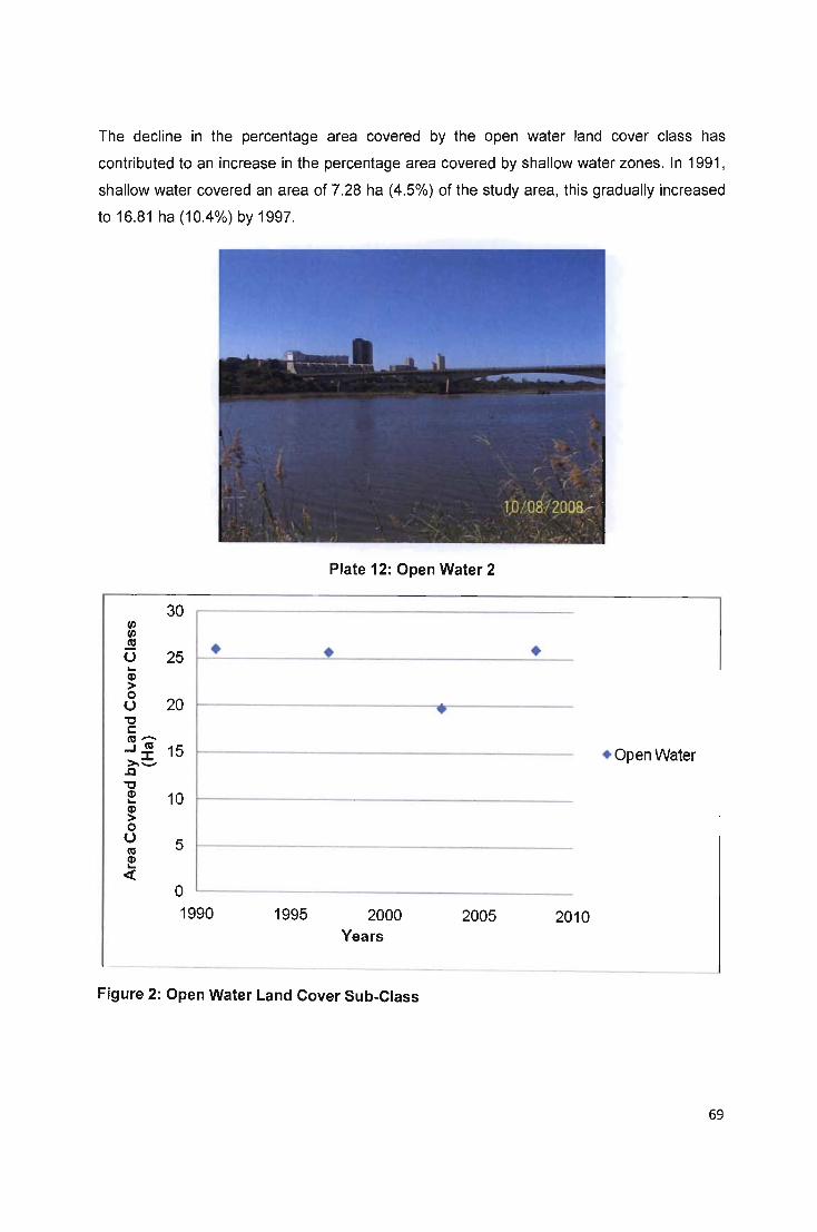
The decline in the percentage area covered by the open water land cover class has
contributed to an increase in the percentage area covered by shallow water zones. In 1991,
shallow water covered an area of 7.28 ha (4.5%) of the study area, this gradually increased
to 16.81 ha (10.4%) by 1997.
30 ", ",
~ • u 25 ... CD > 0
20 u ." t: ttI-..JttI 15 >.~ .Q
." CD 10 ... CD > 0 U 5 ttl
CD ... c:(
0
1990 1995
Plate 12: Open Water 2
•
2000 Years
2005
Figure 2: Open Water Land Cover Sub-Class
•
+ OpenWater
2010
69

.. Q)
> o U
" c
20
18
16
14
12
j ta 10 >.e. .c 8
" ! Q) > o U tV
6
4
2
•
! « o 1990
• •
1995 2000
Years
Figure 3: Shallow Water Land Cover Sub-Class
• Shallow Water
..... T
2005 2010
-----------'
If the correlation coefficient is 0, this means that the changes in the independent and
dependent variable are random and unrelated to one another. In other words no relationship
or bond exists between the variables and thus there is no linear correlation. Figures 2 and 3
both have a correlation coefficient of O. Therefore, it can be assumed that there is no
relationship between the changes in the areas covered by the two water bodies and the time
index.
Currently, shallow water covers 8.63 ha (5.4%) of the Mgeni Estuary and Beachwood
Mangrove Swamp study area. This decline in open water zones is linked to the absence of
regular flushing as a result of significant flooding of the river system and estuary between
1993 and 2008 (Gillard, 2008) . This has been attributed to a controlled release of water by
the water authorities subsequent to the completion of Inanda Dam in 1989 (Garland and
Moleko, 2000).
70
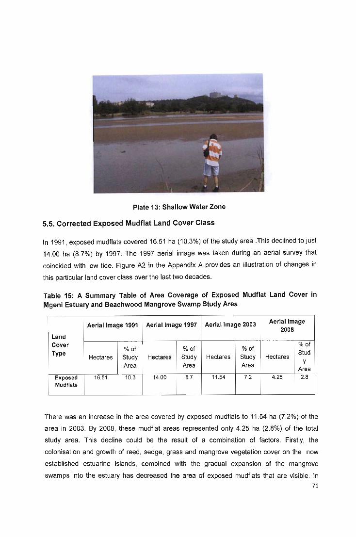
Plate 13: Shallow Water Zone
5.5. Corrected Exposed Mudflat Land Cover Class
In 1991, exposed mudflats covered 16.51 ha (10.3%) of the study area .This declined to just
14.00 ha (8.7%) by 1997. The 1997 aerial image was taken during an aerial survey that
coincided with low tide. Figure A2 in the Appendix A provides an illustration of changes in
this particular land cover class over the last two decades.
Table 15: A Summary Table of Area Coverage of Exposed Mudflat Land Cover in Mgeni Estuary and Beachwood Mangrove Swamp Study Area
Aerial Image 1991 Aerial Image 1997 Aerial Image 2003 Aerial Image 2008
Land Cover
% of % of % of % of
Type Hectares Study Hectares Study Hectares Study Hectares
Stud
Area Area Area y
Area Exposed 16.51 10.3 14.00 8.7 11 .54 7.2 4.25 2.8 Mudflats
There was an increase in the area covered by exposed mudflats to 11.54 ha (7.2%) of the
area in 2003. By 2008, these mudflat areas represented only 4.25 ha (2.8%) of the total
study area. This decline could be the result of a combination of factors. Firstly, the
colonisation and growth of reed, sedge, grass and mangrove vegetation cover on the now
established estuarine islands, combined with the gradual expansion of the mangrove
swamps into the estuary has decreased the area of exposed mudflats that are visible. In
71

addition, tidal fluctuations do have a significant impact on the rise and fall of water levels
within the study area and this could have had an impact on the exposure of mudflats during
the collection of images during the aerial survey process.
20 ii :z:: 18 VI
5: 16 VI III o 14
~ 12 "0 10 c !3 > .Q "0 ~ ~ o v "' CLI ... <t
8
6
4
2
o 1990
................ ~ ~
--------- . ~ ~
1995 2000 2005
Years
•
• Exposed Mudflats
y = -0.6783x + 1368 R2 = 0.8926
2010
----------- ------------------- --------------------------------------------------------------------------------------- ---------- -----------------------------------------------
Figure 4: Decline in the Area Coverage of Exposed Mudflats Land Cover Class
Figure 4 represents the corrected mudflat area values due to tidal variances. It is evident in
the above figure that the area coverage of exposed mudlfats have declined progressively
since 1993. Figure 4 graphically represents a strong negative linear trend with a regession
equation of y= - 0.6783x+1368 with R2 = 0.8926. This indicates a steady decline of exposed
mudflat habitats within the study area between 1991 and 2008.
5.6. Wooded Land Cover Classes
There are several other land cover types that can be identified via aerial imagery and field
surveys. The estuary and mangrove swamps have large areas of densely wooded habitats
consisting of a mixture of indigenous and invasive trees, bushes, vines and shrubs. The
study identified four woody land cover types which were designated as coastal forest,
woodland, mangrove vegetation and island mangrove vegetation.
72

Table 16: A Summary Table of Area Coverage of Wooded Land Cover in Mgeni
Estuary and Beachwood Mangrove Swamp Study Area
Aerial Image 1991 Aerial Image 1997 Aerial Image 2003 Aerial Image
2008 Land Cover
% of % of % of % of Type
Hectares Study Hectares Study Hectares Study Hectares Study Area Area Area Area
Mangrove 24.85 15.4 28.05 17.4 27.82 17.3 29.81 18.4
Island 1.38 0.8 0.52 0.3 1.53 0.9 3.17 2.0 Mangrove
Coastal 7.12 4.4 5.69 5.3 14.07 8.7 18.06 11 .7 Forest
Woodland 4.69 2.9 4.19 2.6 10.91 6.8 8.87 5.5
The researcher has defined coastal forest, for the purpose of this study, as areas with a tree
canopy cover of between 60-100% that consists of indigenous or invasive woody vegetation
(preferably trees). In 1991 this coastal forest covered a 7.12ha (4.4%) of the study area. By
1997 coastal forest had consolidated and expanded its hold, covering an estimated 5.69 ha
(5.3%) of the area as seen in Figure A3 in the Appendix A.
Examination of the 2003 aerial imagery during the course of this study has revealed that the
coastal forest has continued to expand and consolidate its cover within the Beachwood
Mangrove Nature Reserve by encroaching and colonizing areas previously designated as
grassland, scrubland and dune vegetation. It covered approximately 14.07 ha (8.7%) of the
study area in 2003, and without the interference of human harvesting of trees and regular
fires, it currently forms 18.06 ha (11 .7%) of the study area.
Figure 5 below represents the area covered by the coastal forest land cover class plotted
against the time index. The figure shows a strong positive linear trend with a regression
equation of y = 0.5144x -1018.5 and R2 = 0.722. This indicates that coastal forest habitats
are consolidating and gradually expanding throughout the study area.
73
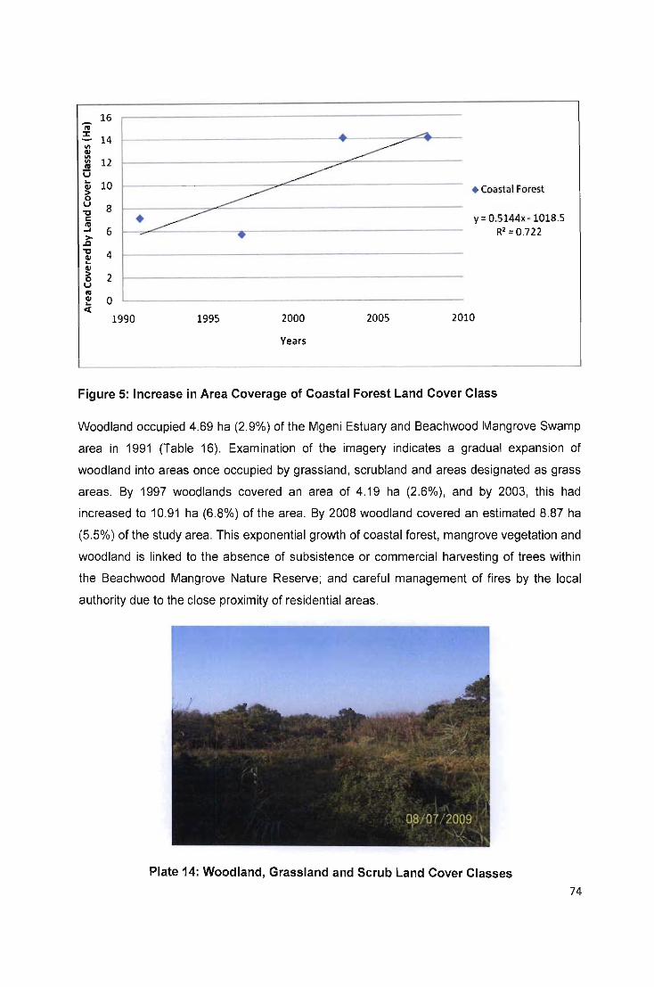
16 'iii =. 14 <1\
" ~ 12 v
~ .~
•
1990 1995
.... ~
~
2000 2005
Years
...-::to..
• Coastal Forest
y :: 0.5 144x - 1018.5 R2 :: 0.722
2010
Figure 5: Increase in Area Coverage of Coastal Forest Land Cover Class
Woodland occupied 4.69 ha (2.9%) of the Mgeni Estuary and Beachwood Mangrove Swamp
area in 1991 (Table 16). Examination of the imagery indicates a gradual expansion of
woodland into areas once occupied by grassland, scrubland and areas designated as grass
areas. By 1997 woodlands covered an area of 4.19 ha (2.6%), and by 2003, this had
increased to 10.91 ha (6.8%) of the area. By 2008 woodland covered an estimated 8.87 ha
(5.5%) of the study area. This exponential growth of coastal forest , mangrove vegetation and
woodland is linked to the absence of subsistence or commercial harvesting of trees within
the Beachwood Mangrove Nature Reserve; and careful management of fires by the local
authority due to the close proximity of residential areas.
Plate 14: Woodland, Grassland and Scrub Land Cover Classes
74

12 Ii • :r:
11\ 10 CII
~. 11\ III /0 0
8 .. ~
CII > 0 • Woodland u
"tJ 6 c
~. /0 ~
Y = 0.3137x · 620.34 > .Il 4 "tJ R2 = 0.532 CII .. CII > 2 0 U III CII .. 0 «
1990 1995 2000 2005 2010
Years
Figure 6: Increase in Area Coverage of Woodland Land Cover Class
Figure 6 above graphically illustrates the increase in the area that is covered by woodland
land cover class within the study area, plotted against the time period . The figure
demonstrates a moderately positive linear trend with the equation 9= 0.3137x - 620.34 and
R2= 0.532.
The second most dominant land cover type within the study area is mangrove forest. This
land cover is dominated by mangrove trees such as Bruguiera gymnorrhiza, and Avicennia
marina . Mangrove vegetation covered an estimated 24.85 ha (15.4%) of the study area in
1991 (Table 16). This woody land cover continued to expand its domination of the estuarine
ecosystem and covered 28.05 ha (17.4%) of the study area by 1997. This expansion has
continued with mangrove vegetation making gradual inroads into areas previously occupied
by coastal forest, grassland , scrubland , salt marshes and dune vegetation. In 2008
mangrove vegetation covered 29.81 ha (18.4%) of the study area as noted in Figure A4
situated in the Appendix.
75

29.50 ii :t: 29.00 1/1 cu 28.50 1/1 1/1 III 0 .. 28.00 .... cu > 27.50 0 1.1 "C 27.00 c !3 > 26.50
.Q
"C 26.00 cu ..
cu > 25.50 0
/ 7
/ 1.1 III
25.00 cu .. ct +
24.50
1990 1995
7 + /
/ + ;7
2000 2005
Years
• Mangrove Vegetation
y = 0.206x· 384.61 R2 = 0.7594
2010
Figure 7: Increase in Area Coverage of Mangrove Forest Land Cover Class
Ii =. 3.50
OIl 3.00 ~ OIl IV v 2.50
~ 8 2.00 "0 C 5 > ~ "0 cu .. ~ IV cu .. ct
1.50
1.00
0.50
0.00
1990
•
----
~ ~ ....
~ ....
1995 2000 2005
Years
• • Island Mangrove
Vegetation
2010
y = 0.108Sx· 215.4 R2 = 0.5196
._ .... _._._._--_ .. _-----------_ .. _ .. _--_ .. _-_._. -----.... _---------- --_._----------------------
Figure 8: Increase in Area Coverage of Island Mangroves Land Cover Class
Figures 7 & 8 both indicate a significant increase in the area coverage of Mangrove Forest
and Island Mangroves Vegetation between 1991 and 2008. This is reflecting in both figures
showing positive linear trends. Figure 7 has a regression equation of y = 0.206x - 384.61
76

and R2 = 0.7594. Meanwhile, Figure 8has an equation of 9= 0.1085x - 215.4 and R 2=
0.5196. Figures 7 & 8 both indicates that the area covered by the mangrove community is
increasing.
Plate 15: Mangrove Vegetation
The Mgeni Estuary is well known for its vegetated islands covered in mangrove tree thickets,
reed beds and grassland habitats. The aerial images show a pattern of colonization,
consolidation and expansion of mangrove vegetation on the islands and mudflats of the
estuary with in the study period . The currents and tidal changes within the estuary carry
mangrove seeds pods and deposit them on mud and sediment area on the islands and
surrounding mudflats (Plate 15). Gradually these seeds germinate and the seedlings
consolidate their position on the islands and form mangrove thickets scattered all over the
islands that consist of a mixture of mature mangrove trees and seedlings. In 1991 mangrove
vegetation had begun to colonize and establish its hold on the eastern islands of the Mgeni
Estuary. Island mangrove vegetation covered about 1.38 ha (0.8%) of the study area at this
stage. Further information is provided in Figure A4 Appendix A.
77

Plate 16: Woodland and Mudflat Land Cover
By 1997 clusters of mangrove trees and seedlings had consolidated their position on the
islands, and soon began to expand throughout the estuary covering 0.52 ha (0.3%) area. In
2003 this land cover dominated 1.53 ha (0.9%) of the study area. In 2008, island mangrove
vegetation covered approximately 3.17 ha (2.0%) of the study area in the absence of human
disturbances, fires, erosion and the flushing of the estuary and river by flooding (Table 16).
This reflects an increase of 1.2 % between 1991 and 2008.
Plate 17: Island Mangrove Vegetation
78
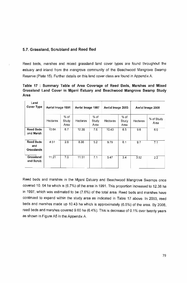
5.7. Grassland, Scrubland and Reed Bed
Reed beds, marshes and mixed grassland land cover types are found throughout the
estuary and inland from the mangrove community of the Beachwood Mangrove Swamp
Reserve (Plate 1S). Further details on this land cover class are found in Appendix A.
Table 17 : Summary Table of Area Coverage of Reed Beds, Marshes and Mixed Grassland Land Cover in Mgeni Estuary and Beachwood Mangrove Swamp Study Area
Land Cover Type Aerial Image 1991 Aerial Image 1997 Aerial Image 2003 Aerial Image 2008
% of % of % of % of Study
Hectares Study Hectares Study Hectares Study Hectares Area
Area Area Area
Reed Beds 10.64 6.7 12.38 7.6 10.43 6.5 9.6 6.0 and Marsh
Reed Beds 4.51 2.8 8.38 5.2 9.79 6.1 9.7 7.1 and
Grasslands
Grassland 11.21 7.0 11.51 7.1 5.47 3.4 3.52 2.2 and Scrub
Reed beds and marshes in the Mgeni Estuary and Beachwood Mangrove Swamps once
covered 10. 64 ha which is (6.7%) of the area in 1991 . This proportion increased to 12.38 ha
in 1997, which was estimated to be (7.6%) of the total area. Reed beds and marshes have
continued to expand within the study area as indicated in Table 17 above. In 2003, reed
beds and marshes made up 10.43 ha which is approximately (6.S%) of the area. By 2008,
reed beds and marshes covered 9.60 ha (6.4%). This is decrease of 0.1 % over twenty years
as shown in Figure AS in the Appendix A.
79

Plate 18: Reed Beds and Marsh
Meanwhile, reed beds and grassland covered 4.51 ha in 1991 . This is around (2.8%) of the
study area (Plate 18). This increased to 8.38 ha (5.2%) of the study area by 1997. In 2008,
reed beds and grassland covered 9.6 ha (6.0%) of the study area. These land covers are
vulnerable to flooding and fires. However, these threats are rare occurrences within the
study area allowing vegetation to expand without hindrance.
Another land cover type which has seen a gradual decline is grassland and scrub. Grassland
and scrub covered 13.21 ha (7.0%) of the study area in 1991, it declined steadily to cover an
area of 11.51 ha (7.1%) by 1997 and by 2003, covered only 5.47 ha (3.4%) of the Mgeni
Estuary and Beachwood Mangrove Swamps. In 2008, this land cover type covered 3.52 ha
(2.2%) of the study area (Table 17). The decline in this land cover type is connected to the
expansion of woody vegetation into areas of the study area that was once covered in
grassland and scrub vegetation. Grassland ecosystems require regular burning to prevent
bush encroachment. However, local authorities control all fires within the study area, and
local conservation officials do not practise a policy of controlled burning of grasslands within
the Beachwood Nature Reserve which would help keep these ecosystems clear of invasive
woody vegetation.
80

16 "iO =. 14 III
~ 12 III iJ
~ ~.
~ ~
1995 2000
Years
~ • ~ .
2005
• Grassland and Scrub
y = -0.6S74x+ 1322.5 R2 = 0.8778
2010
Figure 9: Decline in Area Coverage of Grassland and Scrub Land Cover Class
14 "iO ::E: - 12 III • II • -III III III
10 iJ "-II >
• • • Reed Beds and Marsh 0 8 u
"tJ C III 6 -' 1--------------------_ Y = -O.1311x + 273.24 >
.IJ R2= 0.678
." 4 II "-II > 0 2 v III II "-c( 0
1990 1995 2000 2005 2010
Years
Figure 10: Decline in Area Coverage of Reed Beds and Marsh Land Cover Class
Figures 9 & 10 both represent the area covered by land cover class plotted again the time
period . Both illustrate have a strong negative linear trends. Figure 9 has a regression
equation of y=0.6574x+1322.5 with R2= 0.8778. This shows that this reed bed and marsh
land cover class is declining within the study area. Figure 10 has a regresssion equation of
y= O.1311x + 273.24 and R2= 0.678. This reveals a decline in the area covered by the reed
bed and marsh land cover class within the study area.
81
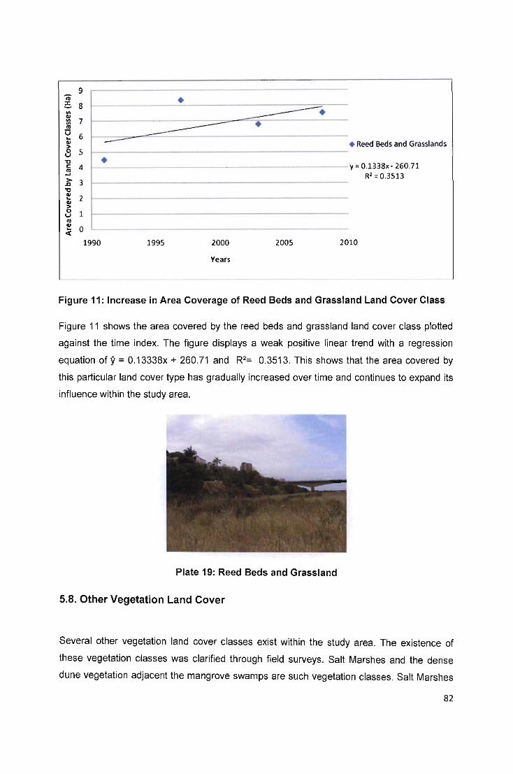
•
-------•
1990 1995 2000
Years
~ . •
2005
• Reed Beds and Grasslands
y :: 0 .1338x · 260.71 R2 = 0.3513
2010
Figure 11: Increase in Area Coverage of Reed Beds and Grassland Land Cover Class
Figure 11 shows the area covered by the reed beds and grassland land cover class plotted
against the time index. The figure displays a weak positive linear trend with a regression
equation of 9 = 0.13338x + 260.71 and R2= 0.3513. This shows that the area covered by
this particular land cover type has gradually increased over time and continues to expand its
influence within the study area.
Plate 19: Reed Beds and Grassland
5.S. Other Vegetation Land Cover
Several other vegetation land cover classes exist within the study area. The existence of
these vegetation classes was clarified through field surveys. Salt Marshes and the dense
dune vegetation adjacent the mangrove swamps are such vegetation classes. Salt Marshes
82

are only found within the Beachwood Mangrove Swamp Reserve and are restricted to a
relatively small location in the centre of the reserve. This habitat has shown signs of decline
over the last couple of decades as other vegetation types such as mangrove vegetation,
grassland and scrubland have expanded and taken over areas previously designated as salt
marsh habitat.
Table 18: A Summary Table of Area Coverage of Other Vegetation Land Cover in
Mgeni Estuary and Beachwood Mangrove Swamp Study Area
Land Cover Aerial Image 1991 Aerial Image 1997 Aerial Image 2003 Aerial Image 2008 Type
%of % of % of % of Hectares Study Hectares Study Hectares Study Hectares Study
Area Area Area Area
Man- 3.07 1.9 3.65 2.2 3.29 2 2.95 1.9 Managed
Grass Area Dune 9.43 5.8 10.46 6.4 12.60 7.8 7.78 5.7
Vegetation
Salt Marsh 1.85 1.1 1.27 0.7 0.68 0.4 0.95 0.6
In 1991 salt marshes covered 1.85 ha (1.1 %) of the study area (Table 18), declining
gradually with the expansion of the grassland, scrubland and mangrove vegetation to a
coverage of 1.27 ha (0.7%) in 1997. Salt marshes covered an area of 0.68 ha (0.4%) in
2003, by 2008 this natural habitat further declined to only cover 0.95 ha (0.6%) of the total
area. See Table 18.These changes are graphically represented in Figure A6 in the Appendix
A.
Dune vegetation is found along the coastline to the east of the mangrove swamps; once
covered approximately 9.43 ha (5.8%) in the early 1990s. This vegetation type currently
covers 8.78 ha (5.4%) of the study area due to the destructive nature of recent high tides,
wind erosion and human activity that has removed and steady thinned out the dune
vegetation.
83

'ii =. III
~ VI III U .. GI :> 0 v '0 C III -' >
.&:I '0 GI .. GI :> 0 v III GI .. "'
14
12
10
8
6
4
2
o 1990
•
• •
•
1995 2000 2005
Years
Figure 12: Area Coverage of Dune Vegetation Land Cover Class
2 'ii =. 1.8 III
~ 1.6 III U 1.4 .. GI
~ 1.2 v -g 1 ~ > 0.8 .Q
'0 0.6 ~ ~ 0.4
III 0.2 GI .. "' 0
1990
• --- ------~ ------ ------- •
• -----
1995 2000 2005
Years
2010
• Dune Vegetation
. SaltMarsh
y = -0.0628x + 126.67 R2 =0.8036
2010
Figure 13 : Decline in the Area Coverage of Salt Marsh Land Cover Class
Figures 12 represents the area covered by the dune vegatation land cover class poltted
againts the time period of the study. The figure indicates that this land cover class has only
changed slightly but otherwise has remained relativelly constant over the established time
period. Figure 13 illustrates area covered by the Salt Marsh land cover class against the time
84

index. The figure displays a strong negative linear trend ,and the regression equation for this
figure is y= - 0.0628x + 126.67 and R2 = 0.8036. This indicates a steady decline in the area
coverage of Salt Marsh habiats within the study area.
Plate 20: Salt Marsh
Man-Managed Grass Areas within the study area covered 3.07 ha (1.9%) of the study area
in 1991. This gradually increased to 3.65 ha (2.2%) by 1997. However, this land cover
declined gradually and only covered 2.95 ha (1.8%) of the area by 2008. This decline is
largely due to the increase in areas of development within the study area and the expansion
of woodland into areas previously designated as grass areas. The changes in the area
covered by this land cover class can be seen in Figure A7 in the Appendix.
Plate 21: Transission from Salt Marsh to Mangrove Vegetation
85
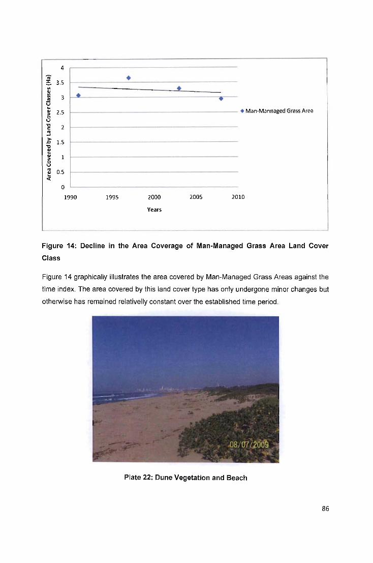
4
ii • ~ 3.5 '" • CII ::I 3 • III • 0 .. CII 2.5 > 1-------------------- • Man-Mannaged Grass Area 0 V "0 2 c III .... > 1.5 Sl
"0 CII .. CII 1 > 0 V 10 0.5 CII .. ct
0
1990 1995 2000 2005 2010
Years
Figure 14: Decline in the Area Coverage of Man-Managed Grass Area Land Cover
Class
Figure 14 graphically illustrates the area covered by Man-Managed Grass Areas against the
time index. The area covered by this land cover type has only undergone minor changes but
otherwise has remained relativelly constant over the established time period.
Plate 22: Dune Vegetation and Beach
86

5.9. Other Land Cover Classes
There are several other land cover types that exist within the Mgeni Estuary and Beachwood
Mangrove Swamp study area that require examination.
Table 19: A Summary Table of Area Coverage of Other Land Cover Classes in Mgeni Estuary and Beachwood Mangrove Swamp Study Area
Aerial Image 1991 Aerial Image 1997 Aerial Image 2003 Aerial Image 2008
Land Cover Type % of % of % of % of
Hectares Study Hectares Study Hectares Study Hectares Study Area Area Area Area
Sand Bank 5.46 3.3 4.42 2.7 4.29 2.6 8.75 5.4
Beach 18.67 11.5 16.38 10.1 13.04 8.1 11 .23 7.0
Conservation 1.13 0.7 0.92 0.5 1.36 0.8 1.39 0.8 Managed
Area
The sandbanks found in the vicinity of the Mgeni estuary mouth covered 5.46 ha (3.3%) of
the study area in 1991, but declined steadily to cover an area of approximately 4.4211 ha
(2.7%) of the total area by 1997. By 2003 sandbanks only covered 4.29 ha (2.6%). By 200S
sandbanks covered S.75 ha (5.4%).This represents an increase of 2.1 % over the last couple
of decades. These changes can be observed in Figure AS in Appendix A.
Plate 23: Sand Banks at Estuary Mouth
87
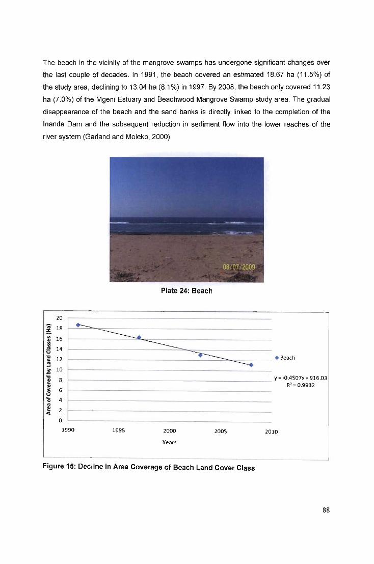
The beach in the vicinity of the mangrove swamps has undergone significant changes over
the last couple of decades. In 1991 , the beach covered an estimated 18.67 ha (11 .5%) of
the study area, declining to 13.04 ha (8.1 %) in 1997. By 2008, the beach only covered 11.23
ha (7.0%) of the Mgeni Estuary and Beachwood Mangrove Swamp study area. The gradual
disappearance of the beach and the sand banks is directly linked to the completion of the
Inanda Dam and the subsequent reduction in sediment flow into the lower reaches of the
river system (Garland and Moleko, 2000).
Plate 24: Beach
20
iii 18 +--:E: =------. -III 16 5t ----III fU 14 v
~ "0 12 + Seach c fU --.. .... >- 10 ..a
"0 8 Y = -O.4507x + 916.03 cu ...
R2 = 0.9932 cu > 6 0 u - 4 0 fU cu 2 ... <
0
1990 1995 2000 2005 2010
Years
Figure 15: Decline in Area Coverage of Beach Land Cover Class
88

9 ii :r:: 8 1/1 Q/
::: 7 ~ o ~ 6 > 8 5 "D c:: .!3 4 ~ "D 3 Q/ ... Q/ .3 2
~ 1 < o
1990
• ---- • •
1995 2000
Year
• --
2005
+ SandBank
y = 0.105x · 204.5 R2 = 0.2475
2010
Figure 16: Increase in Area Coverage of Sand Bank Land Cover Class
Figure 15 illustrates the area covered by the beach land cover class within the study area
against the established time period of the study. Examination of the figure reveals the
existence of a strong negative linear trend with a regression equation of y= - 0.4507x +
916.03 and R2 = 0.9932. This indicates that the land cover class is showing signs of decline.
Meanwhile, Figure 16 shows the area covered by the sand banks land cover class plotted
against the time period . There is a moderately positive linear trend that has a regression
equation of y= 0.105x + 204.5 and R2 = 0.2475. This reveals that the area covered by this
land cover class is increasing steadily within the study area.
Plate 25: Sand Banks
89
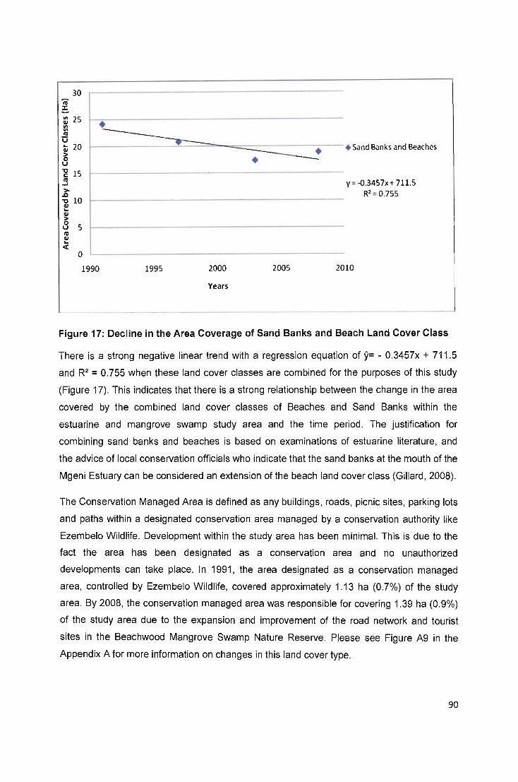
'iii :z: -
30
~ 25 ~ III • V .. 20
~ I-______ ..:!:.-'Y _-==--'""'""'--;----!==-.------=.--. Sand Banks and Beaches
-g 15 .!3 ~ "tI 10 ~ G/ > 8 5 III G/ .. < o
1990 1995 2000
Years
2005
y = -o.3457x+ 711.5 R2 = 0.755
2010
Figure 17: Decline in the Area Coverage of Sand Banks and Beach Land Cover Class
There is a strong negative linear trend with a regression equation of y= - 0.3457x + 711.5
and R2 = 0.755 when these land cover classes are combined for the purposes of this study
(Figure 17). This indicates that there is a strong relationship between the change in the area
covered by the combined land cover classes of Beaches and Sand Banks within the
estuarine and mangrove swamp study area and the time period. The justification for
combining sand banks and beaches is based on examinations of estuarine literature, and
the advice of local conservation officials who indicate that the sand banks at the mouth of the
Mgeni Estuary can be considered an extension of the beach land cover class (Gillard, 2008).
The Conservation Managed Area is defined as any buildings, roads, picnic sites, parking lots
and paths within a designated conservation area managed by a conservation authority like
Ezembelo Wildlife . Development within the study area has been minimal. This is due to the
fact the area has been designated as a conservation area and no unauthorized
developments can take place. In 1991 , the area designated as a conservation managed
area, controlled by Ezembelo Wildlife, covered approximately 1.13 ha (0.7%) of the study
area. By 2008, the conservation managed area was responsible for covering 1.39 ha (0.9%)
of the study area due to the expansion and improvement of the road network and tourist
sites in the Beachwood Mangrove Swamp Nature Reserve. Please see Figure A9 in the
Appendix A for more information on changes in this land cover type.
90
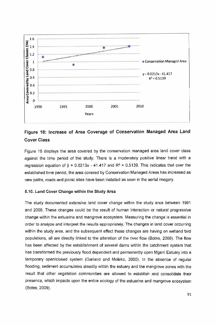
1.6 ii =- 1.4 '" 5: a 1.2 • ______
ti 1 ~=:::::::...----------------- + Conservation Managed Area ~ . v "'D 0.8 c ftI
~0.6 .lJ "'D ~ 0.4
~ v 0.2 ftI
~ 0
"' 1990 1995
-----_._-_._-_._.
2000 2005
Years
y = 0.0213x - 41.417 R2 = 0.5139
2010
Figure 18: Increase of Area Coverage of Conservation Managed Area Land
Cover Class
Figure 18 displays the area covered by the conservation managed area land cover class
against the time period of the study. There is a moderately positive linear trend with a
regression equation of y = 0.0213x - 41.417 and R2 = 0.5139. This indicates that over the
established time period, the area covered by Conservation Managed Areas has increased as
new paths, roads and picnic sites have been installed as seen in the aerial imagery.
5.10. Land Cover Change within the Study Area
The study documented extensive land cover change within the study area between 1991
and 2008. These changes could be the result of human interaction or natural progressive
change within the estuarine and mangrove ecosystem. Measuring the change is essential in
order to analyze and interpret the results appropriately. The changes in land cover occurring
within the study area, and the subsequent effect these changes are having on wetland bird
populations, all are directly linked to the alteration of the river flow (Botes, 2009). The flow
has been affected by the establishment of several dams within the catchment system that
has transformed the previously flood dependent and permanently open Mgeni Estuary into a
temporary open/closed system (Garland and Moleko, 2000). In the absence of regular
flooding, sediment accumulates steadily within the estuary and the mangrove zones with the
result that other vegetation communities are allowed to establish and consolidate their
presence, which impacts upon the entire ecology of the estuarine and mangrove ecosystem
(Bates, 2009).
91
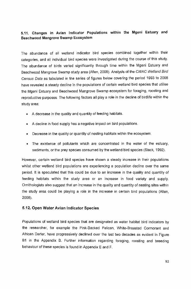
5.11. Changes in Avian Indicator Populations within the Mgeni Estuary and Beachwood Mangrove Swamp Ecosystem
The abundance of all wetland indicator bird species combined together within their
categories, and all individual bird species were investigated during the course of this study.
The abundance of birds varied significantly through time within the Mgeni Estuary and
Beachwood Mangrove Swamp study area (Allen, 2008). Analysis of the CWAC Wetland Bird
Census Data as tabulated in the series of figures below covering the period 1993 to 2008
have revealed a steady decline in the populations of certain wetland bird species that utilise
the Mgeni Estuary and Beachwood Mangrove Swamp ecosystem for foraging , roosting and
reproductive purposes. The following factors all playa role in the decline of birdlife within the
study area:
• A decrease in the quality and quantity of feeding habitats.
• A decline in food supply has a negative impact on bird populations.
• Decrease in the quality or quantity of nesting habitats within the ecosystem.
• The existence of pollutants which are concentrated in the water of the estuary,
sediments, or the prey species consumed by the wetland bird species (Slack, 1992).
However, certain wetland bird species have shown a steady increase in their populations
whilst other wetland bird populations are experiencing a population decline over the same
period . It is speculated that this could be due to an increase in the quality and quantity of
feeding habitats within the study area or an increase in food variety and supply.
Ornithologists also suggest that an increase in the quality and quantity of nesting sites within
the study area could be playing a role in the increase in certain bird populations (Allen,
2008).
5.12. Open Water Avian Indicator Species
Populations of wetland bird species that are designated as water habitat bird indicators by
the researcher, for example the Pink-Backed Pelican , White-Breasted Cormorant and
African Darter, have progressively declined over the last two decades as evident in Figure
B1 in the Appendix B. Further information regarding foraging , roosting and breeding
behaviour of these species is found in Appendix E and F.
92
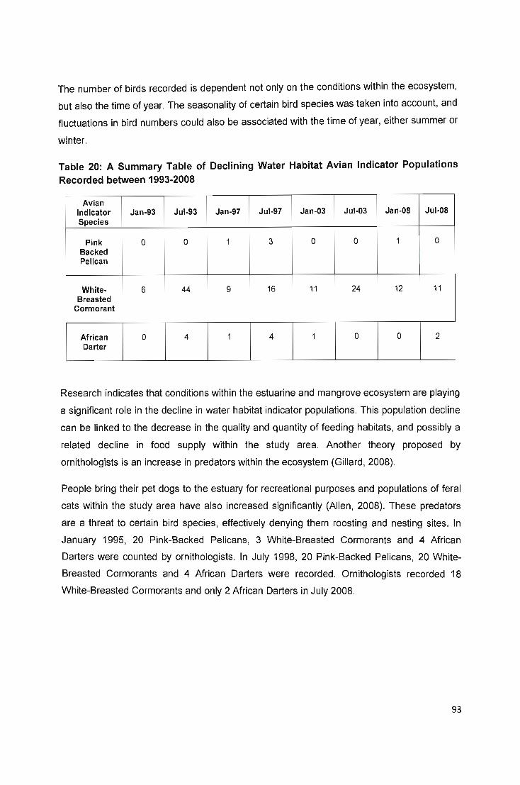
The number of birds recorded is dependent not only on the conditions within the ecosystem,
but also the time of year. The seasonality of certain bird species was taken into account, and
fluctuations in bird numbers could also be associated with the time of year, either summer or
winter.
Table 20: A Summary Table of Declining Water Habitat Avian Indicator Populations Recorded between 1993-2008
Avian Indicator Jan-93 Jul-93 Jan-97 Jul-97 Jan-03 Jul-03 Jan-OS Jul-OS Species
Pink 0 0 1 3 0 0 1 0 Backed Pelican
White- 6 44 9 16 11 24 12 11 Breasted
Cormorant
African 0 4 1 4 1 0 0 2 Darter
Research indicates that conditions within the estuarine and mangrove ecosystem are playing
a significant role in the decline in water habitat indicator populations. This population decline
can be linked to the decrease in the quality and quantity of feeding habitats, and possibly a
related decline in food supply within the study area. Another theory proposed by
ornithologists is an increase in predators within the ecosystem (Gillard, 2008).
People bring their pet dogs to the estuary for recreational purposes and populations of feral
cats within the study area have also increased significantly (Allen, 2008). These predators
are a threat to certain bird species, effectively denying them roosting and nesting sites. In
January 1995, 20 Pink-Backed Pelicans, 3 White-Breasted Cormorants and 4 African
Darters were counted by ornithologists. In July 1998, 20 Pink-Backed Pelicans, 20 White
Breasted Cormorants and 4 African Darters were recorded. Ornithologists recorded 18
White-Breasted Cormorants and only 2 African Darters in July 2008.
93
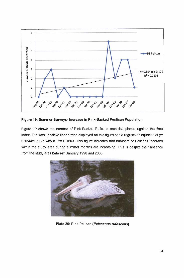
"0 tI "0 ... 0 U tI a:: \II "0 ... iii .... 0 ... tI
J:I E :J Z
7
6
5
4
3
2
1
0
..... PBPelican
v = 0.1544x + 0.125 R2= 0.1503
Figure 19: Summer Surveys-Increase in Pink-Backed Peclican Population
Figure 19 shows the number of Pink-Backed Pelicans recorded plotted against the time
index. The weak positive linear trend displayed on this figure has a regression equation of 9= 0.1544x+O.125 with a R2= 0.1503. This figure indicates that numbers of Pelicans recorded
within the study area during summer months are increasing. This is despite their absence
from the study area between January 1998 and 2003.
Plate 26: Pink Pelican (Pe/ecanus rufescens)
94
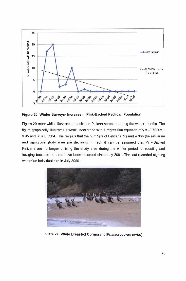
25
"C QI 20 "C .. 0 U QI -+-PB Pelican a: <II 15 "C .. iD -0 .. QI 10 .l:I Y = ·0.7809x + 9.95 E
Rl : 0.3304 ::s z
Figure 20: Winter Surveys- Increase in Pink-Backed Peclican Population
Figure 20 meanwhile, illustrates a decline in Pelican numbers during the winter months. The
figure graphically illustrates a weak linear trend with a regression equation of 9 = -0.7809x +
9.95 and R2 = 0.3304. This reveals that the numbers of Pelicans present within the estuarine
and mangrove study area are declining. In fact, it can be assumed that Pink-Backed
Pelicans are no longer utilising the study area during the winter period for roosting and
foraging because no birds have been recorded since July 2001. The last recorded sighting
was of an individual bird in July 2000.
Plate 27: White Breasted Cormorant (Pha/acrocorax carbo)
95
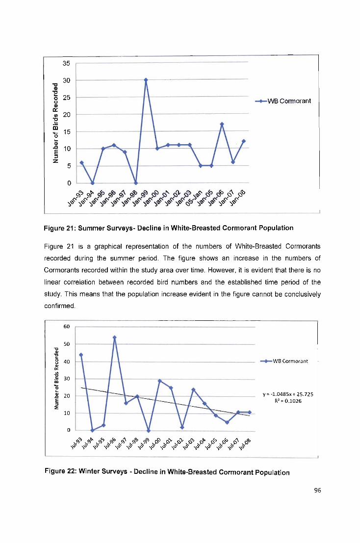
35
30 "0 G> "0 ... 25 0 ....... WB Cormorant (J G>
£t: til 20
"0 .: m
15 -0 ... G> .0 10 E ::1 Z
5
0
Figure 21: Summer Surveys- Decline in White-Breasted Cormorant Population
Figure 21 is a graphical representation of the numbers of White-Breasted Cormorants
recorded during the summer period. The figure shows an increase in the numbers of
Cormorants recorded within the study area over time. However, it is evident that there is no
linear correlation between recorded bird numbers and the established time period of the
study. This means that the population increase evident in the figure cannot be conclusively
confirmed.
60
50 'll QI 'll ... 0 40 u QI
ex: III
'E 30 iii -0 ... .! 20 E :::J Z
10
0
....... WB Cormorant
y = -1 .0485x+ 25.725 R~ = 0.1026
Figure 22: Winter Surveys - Decline in White-Breasted Cormorant Population
96

The Figure 22 displays the number of birds recorded within the study area plotted against
the time period. The figure shows a weak negative linear trend and a regression equation of
y= -1.0485x + 25.725 of R2 = 0.1026. If there is a negative correlation coefficient like -0.1026
this means that the two variables will respond in opposite directions. While the one
increases, the other variable will decrease. Therefore, as time increases the population
of Cormorants is declining. Careful analysis of the entire time period indicates an overall
population decline as displayed in Figure C1 found in the Appendix C.
4.5
4
3.5 "g tI
3 "g .. 0 u tI 2.5 a:: CII "g
2 .. iii
\
\ .... 0
1.5 .. J E 1 ::J Z
O.S
0
1.. .... ....
~ !\ .... ..J \ ~ .... .... .... .... -----...-:
10."'0.'> I>~ ",fo ~~ ",'b ~ _,,"-,,'\. ~", ~"'~ r-~ I'\fo ('~ I'\'b
Figure 23: Summer Surveys- Decline in African Darter Population
...... African Darter
y:: -o.0809x + 1.125 Rl :: 0.1396
Figures 23 shows a weak negative linear trend with an equation of y= -0.0809x+1.125 with a
R2= 0.1396. This indicates a weak relationship between the number of birds recorded and
the time period. No birds were recorded during surveys between January 1999 and January
2002. In later years the species seems to have disappeared from the study area during the
summer months.
Figure 24 illustrates the number of African Darter recorded during the winter months of the
year. This figure indicates that the number of birds recorded during the winter months is
declining. However, there is no linear correlation between the variables. This makes it
difficult to confirm there is a relationship between the variables, the number of birds recorded
and the time period.
97
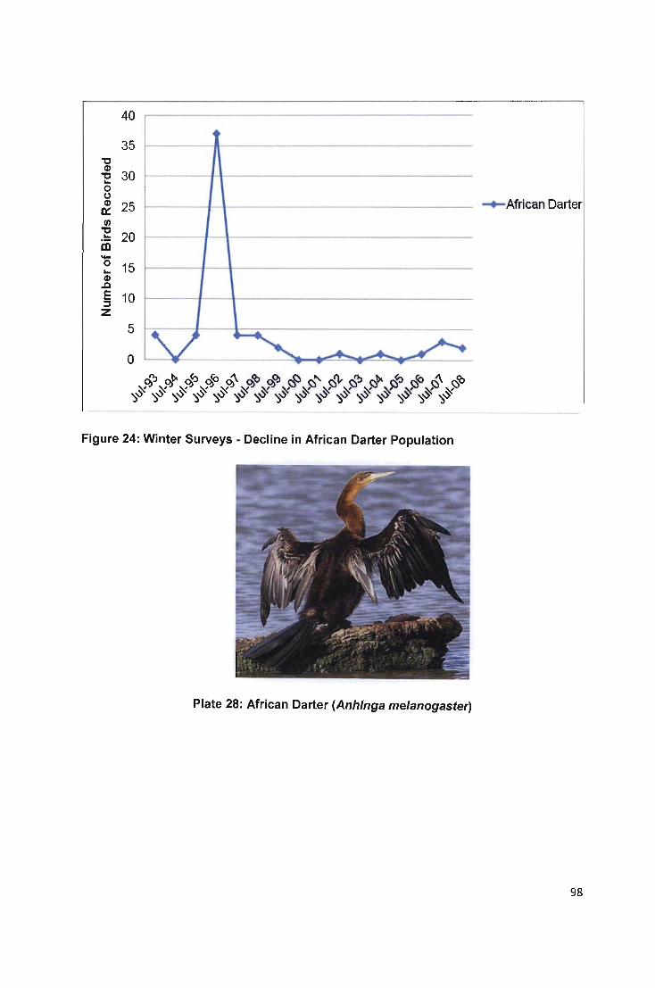
40
35 "0 cP
30 "0 .... 0 (,) cP 25 0:: -+-African Darter f1J "0
20 .... iii '0 15 .... cP
.Q E 10 :::J Z
5
0 v ~ ....... ...... ~ '" ..
Figure 24: Winter Surveys - Decline in African Darter Population
Plate 28: African Darter (Anhinga melanogaster)
98
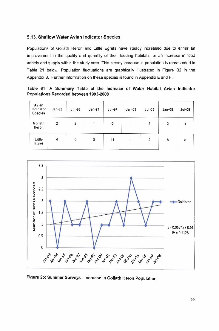
5.13. Shallow Water Avian Indicator Species
Populations of Goliath Heron and Little Egrets have steady increased due to either an
improvement in the quality and quantity of their feeding habitats, or an increase in food
variety and supply within the study area. This steady increase in population is represented in
Table 21 below. Population fluctuations are graphically illustrated in Figure B2 in the
Appendix B. Further information on these species is found in Appendix E and F.
Table 61: A Summary Table of the Increase of Water Habitat Avian Indicator Populations Recorded between 1993-2008
Avian Indicator Jan-93 Jul-93 Jan-97 Jul-97 Jan-03 Jul-03 Species
Goliath 2 2 1 0 1 5 Heron
Little 4 0 0 11 1 2 Egret
3.5
3
" " " 2.5 I... 0 U
" a: 2 1/1
" I...
iii ... 1.5 0 I...
" .a E 1 ~ z
0.5
0
Figure 25: Summer Surveys - Increase in Goliath Heron Population
Jan-OS Jul-OS
2 1
8 8
~GoHeron
y= 0.0574x+ 0.95 R2 = 0.1125
99
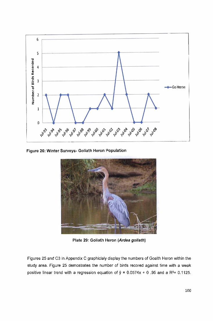
6
5
"C GI "C ..
4 0 u GI a:: 11\ "C
3 .. Cii ...
..... GoHeron 0 .. GI
2 .Q
E :J Z
1
0
Figure 26: Winter Surveys- Goliath Heron Population
Plate 29: Goliath Heron (Ardea goliath)
Figures 25 and C3 in Appendix C graphiclaly display the numbers of Goaith Heron within the
study area. Figure 25 demostrates the number of birds recored against time with a weak
positive linear trend with a regression equation of 9 = 0.0574x + 0 .95 and a R2= 0.1125.
100

This indicates that Goliath Heron numbers have steadily increased over the time period of
the study.
Meanwhile, Figure 26 reflects the number of Goliath Herons recorded plotted against the
time period. This figure indicates that there is no connection between the variables. The
fluctuations in bird numbers were too inconsistent to determine if they were statistically
relevant.
Apparent human error during the CWAC Wetland Bird Census could be responsible for
inconsistencies in certain avian data sets. Below, Figure 27 displays a positive linear trend in
favour of a general Little Egret population increase over the summer periods since the
induction of the CWAC Wetland Avian Census.
Figure 27 below indicates a weak positive linear trend with a regression equation of 9= 0.2515x + 1.8 and R2= 0.1353. Therefore, a change in the independent variable should
result in a comparable increase or decrease in the dependent variable. Therefore, as time
increases there is a comparable increase in the population of Little Egrets in the study area.
Figure 28 just reflects the number of Little Egrets recorded during the winter time period.
However,
details.
12
10
~ C1I -e 8 0 u C1I
0:::
'" ~ .... 6 iii -0 .... ~ 4 E :J Z
2
0
no linear correlation was established. See Figure C4 in Appendix C for more
-+-L Egret
y = 0 .2515x+ 1.8 R2= 0 .1353
Figure 27:Summer Surveys - Increase in Little Egret Population
101
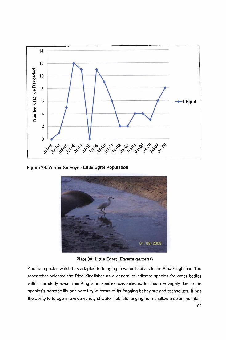
14
12 "t:I Q)
"t:I 10 ... 0 (J Q)
0:: 8 '" "t:I
.!:: m '0 6 -+-L Egret ... Q)
.Q
E 4 ;:, z
2
0
------------------- --
Figure 28: Winter Surveys - Little Egret Population
Plate 30: Little Egret (Egretta garzetta)
Another species which has adapted to foraging in water habitats is the Pied Kingfisher. The
researcher selected the Pied Kingfisher as a generalist indicator species for water bodies
within the study area. This Kingfisher species was selected for this role largely due to the
species's adaptability and versitlity in terms of its foraging behaviour and technqiues. It has
the ability to forage in a wide variety of water habitats ranging from shallow creeks and inlets
102
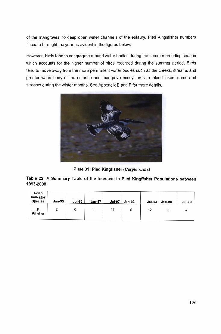
of the mangroves, to deep open water channels of the estaury. Pied Kingsfisher numbers
flucuate throught the year as evident in the figures below.
However, birds tend to congregate around water bodies during the summer breeding season
which accounts for the higher number of birds recorded during the summer period. Birds
tend to move away from the more permanent water bodies such as the creeks, streams and
greater water body of the esturine and mangrove ecosystems to inland lakes, dams and
streams during the winter months. See Appendix E and F for more details.
Plate 31: Pied Kingfisher (Cery/e rudis)
Table 22: A Summary Table of the Increase in Pied Kingfisher Populations between 1993-2008
Avian Indicator Species Jan·93 Jul·93 Jan·97 Jul·97 Jan·03 Jul·03 Jan·OB Jul·OB
p 2 0 1 11 0 12 3 4 K1fisher
103

8
7
"0 6 ~
"0 ~
0 u 5 ~ a: III
"0 ~ 4 iii -0 ~ 3 ~
..0 E :J 2 z
1
0
Figure 29: Summer Surveys - Increase in Pied Kingfisher Population
...... PK/fisher
y :: 0.2853x · 0.175 R2 :: 0.3898
Examination of the figures indicates a significant increase in Pied Kingfisher numbers within
the summer periods, and a slight decline in bird numbers over the winter period. The
reasons for such population flucuations have been discussed above. Figure 29 shows a
modertly positive linear trend with a regression equation of y= 0.2853x + 0.175 and a R2= 0.3898. It is clearly evident that Kingfisher numbers are increasing during the summer
period.
Figure 30 displays the number of Pied Kingfishers recorded plotted against time. However,
there is no linear correlation between the values. Further information regarding the increase
in the numbers of kingfishers recorded within the study area can be found in Figure 83 and
C6 in the Appendix 8 and C.
104

14
12
"0 CII 10 "0 .. 0 u CII a:: 8 III "0 .. iii - 6 -+-P K/fisher 0 .. .8 E 4 ~ z
2
0
Figure 30: Winter Surveys - Pied Kingfisher Population
The Pied Kingfisher population has increased significantly over the last two decades.
population growth is largely due to an increase in food supply, and possibly an improvement
in terms of quality and quantity of foraging and nesting habitats within the study area.
5.14. Mudflat Avian Indicator Species
Ornithologists have recorded a gradual decline in wading bird species within the study area
during the past couple of decades. The researcher decided to designate these bird species
as mudflat indicators because of their reliance on mudflats for foraging and roosting.
Table 23: A Summary Table of the Number of Mudflat Avian Indicators Recorded between 1993-2008
Avian Indicator Species Jan-93 Jul-93 Jan-97 Jul-97 Jan-03 Jul-03 Jan-08 Jul-08
Sacred Ibis 8 72 119 110 107 10 9 4
Sanderling 0 0 0 0 60 0 97 0
Curlew 224 0 170 0 0 0 162 S/piper 0
L Stint 138 0 38 0 61 0 3 0
BS Plover 15 49 54 45 98 60 91 82
105
The study revealed a decline in the number of Little Stints, Curlew Sandpipers and Sacred
Ibis recorded within the Mgeni Estuary and Beachwood Mangrove Swamp Study Area. The
decline in Sacred Ibis populations is illustrated in Figure B4 in Appendix B. The decrease in
wading bird populations could be due to predation , disease or the reduction in the quality
and quantity of feeding and roosting habitats within the study area (Slack, 1992). However,
this is just pure speculation until further research can be conducted.
Despite the decline in certain indicator populations, Sanderling numbers have increased
from no recorded sightings within the study area during the early 1990s, to 97 birds in
January 2008 as evident in the Table 23 above. Figure 32 below has a weak positive linear
trend with a regression equation 9= 3.1985x + 3.875 and a R2 = 0.257. This indicates that
the number of Sanderlings visiting the Mgeni Estuary and Beachwood Mangrove Swamps is
increasing.
This increase in numbers of Sanderlings visiting the Mgeni Estuary and Beachwood
Mangrove Swamps could be due to the following:
• A decline in the populations of competing species of wading birds such as Little
Stints and Curlew Sandpipers. Less competition in terms of foraging and roosting
locations and abundance in prey species contributes to an increase in Sanderling
numbers (Gillard, 2008).
• An increase in the abundance of preferred prey species within the Mgeni Estuary and
Beachwood Mangrove Swamp Study area. In addition, an increase in the abundance
of preferred roosting and suitable foraging habitats could be another influencing
factor (Allen, 2008).
• A decline in predator species within the study area.
• A decline in the quality and quantity of other previously suitable roosting and foraging
habitats in vicinity of other water bodies encouraging birds to use study area.
106
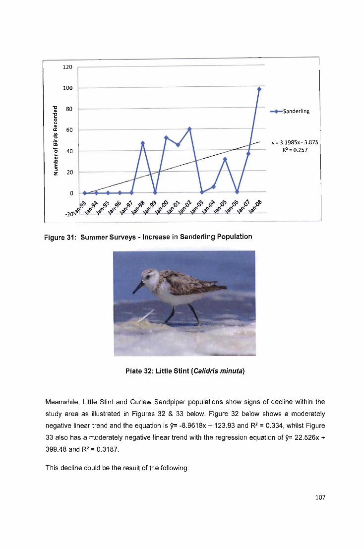
120
100
'tJ 80 QI 'tJ ... 0 u QI a: 60 III 'tJ ... iii - 40 0 ... QI .D E :::J 20 z
0
Figure 31: Summer Surveys - Increase in Sanderling Population
Plate 32: Little Stint (Calidris minuta)
...... Sanderling
y :: 3.1985x - 3.875 R2 :: 0.257
Meanwhile, Little Stint and Curlew Sandpiper populations show signs of decline within the
study area as illustrated in Figures 32 & 33 below. Figure 32 below shows a moderately
negative linear trend and the equation is 9= -8 .9618x + 123.93 and R2 = 0.334, whilst Figure
33 also has a moderately negative linear trend with the regression equation of 9= 22.526x +
399.48 and R2 = 0.3187.
This decline could be the result of the following :
107
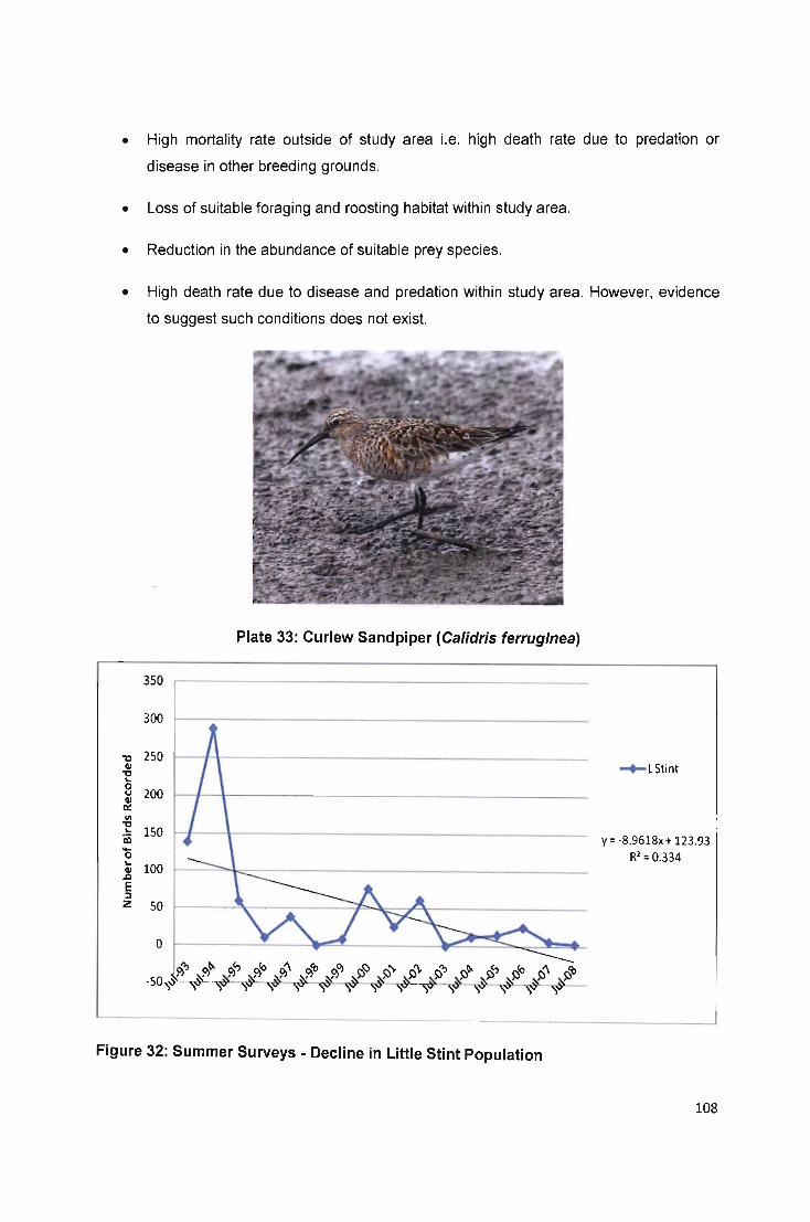
• High mortality rate outside of study area i.e. high death rate due to predation or
disease in other breeding grounds.
• Loss of suitable foraging and roosting habitat within study area.
• Reduction in the abundance of suitable prey species.
• High death rate due to disease and predation within study area. However, evidence
to suggest such conditions does not exist.
Plate 33: Curlew Sandpiper (Calidris ferruginea)
350
300
'tI 250 CII 'tI .. 0
200 u CII a:: III 'tI
150 .. iii .... 0 .. 100 CII
.D. E ::I Z 50
0
Figure 32: Summer Surveys - Decline in Little Stint Population
-+-LStint
y = -8.9618x + 123.93 R2 = 0.334
108

700
600 "0 III "0 500 .. 0 U III ex: 400 III "0 .. iii ... 300 0 .. III
.D. E 200 :l Z
100
0
Figure 33: Summer Surveys - Decline in Curlew Sandpiper Population
-+-Curlew S/piper
y = -22.S26x + 399.48 R2 = 0.3187
Sacred Ibis populations have also shown signs of population fluctuations over the last couple
of decades. In 1993 ornithologists recorded the presence of +/- 100 Ibises within the study
area during five separate surveys.
Plate 34: Sacred Ibis (Threskiornis aethiopicus)
Numbers grew substantially within the study area following the establishment of a breeding
and roosting colony on the grounds of the Umgeni River Bird Park during 1996/97
(Gillard,2008). However, the Ibises were responsible for the spreading of a highly contagious
and lethal bactericidal infection through the park's captive water bird population through their
faeces. Park management implemented a programme to remove the Ibis colony and prevent
109

birds from settling on the grounds in large numbers in mid-2003 (Allen, 2008). The decline in
the population of Sacred Ibises over the last two decades can be seen in Figure C2 of
Appendix C.
140
120 "0
" "0 100 ... 0 u
" a: 80 til "0 ... m ... 60 .....Sacred Ibis 0 ... " .a E 40 :J Z
20
0
Figure 34: Summer Surveys - Increase in Sacred Ibis Population
Figure 34 illustrates that there is no relationship between the dependent and independent
variables and thus there is no linear correlation . However, the peaks in the Ibis population
displayed in 1997/98, 2002/03 and 2007/08 could be due to the abundance of prey species
and an increase in suitable foraging locations within the study area during the summer
months. In addition, ornithologists indicate that Sacred Ibises will congregate in large
numbers near water bodies surrounded by tall trees and other vegetation as such areas are
ideal for the establishment of breeding colonies. Prior to the removal of the Ibis breeding
colony from the Umgeni River Bird Park property in 2003, most of the Ibises recorded during
CWAC Wetland Avian Censuses within the Mgeni Estuary and Beachwood Mangrove
Swamp study area, were adult birds from the breeding colony situated in the bird park
grounds that were vigorously foraging to ensure a constant supply of sustenance to raise
their chicks. It was assumed that the establishment of a new breeding colony on the
adjacent golf course on the south bank of the estuary during 2006/2007 period would
eventually lead to a gradual recovery of the Sacred I bis population in the area.
Figure 35 below, representing the numbers of Ibises recorded within the study area during
the winter months, indicates a weak negative linear trend with an equation of 9= -4.838x +
110

114.05 with the R2 = 0.2302. This figure displays a population decline during the winter
period .
250
"0 200 GI "0 ... 0 U GI 150 a:: III "0 ... iii ... 0 100 ... GI .t:I E :l Z 50
0
Figure 35: Winter Surveys - Decline in Sacred Ibis Populations
-+-Sacred Ibis
y = -4.9838x + 114.05 R2 = 0.2302
However, the gradual decline in Ibis populations during the winter period shown in Figure 35
is representative of a general Sacred Ibis population decline within the Mgeni Estuary and
adjacent Beachwood Mangrove Swamps over the last two decades. Ibis numbers within the
study area show signs of a steady decline after the implementation of this Umgeni River Bird
Parks removal programme, as birds moved to other more suitable breeding, roosting and
feeding areas around the Durban area and have not return. For example, Ibises have
recently established a breeding colony in Durban Botanical Gardens. This population decline
is illustrated in the Figure C2 which can be found in the Appendix C.
111

120
100
'0 QI '0 ... 80 0
-+- BS Plover u QI a: OIl '0
60 ... iii -0 ... .8 40 E
1-----;;;>""q -----lH --------------'f = 4.4324x + 23.325
::J R2: 0.3988
Z
20
0
Figure 36: Summer Surveys - Increase in Black-Smith Plover Population
The Blacksmith Plover population increased steadily between 1993 and 2008. Figure 36
illustrates the number of birds recorded plotted against the time index and shows a
moderately positive linear trend with a regression equation of y= 4.4324x + 23.325 and R2= 0.3988.
90
80
'0 70 QI '0 o 60 u QI a: OIl 50 '0 ... iii '0 40 ... QI
.t:I 30 E ::J
Z 20
10
o
Figure 37: Winter Surveys - Increase in Black-Smith Plover Population
....... BSPlover
y = 1.2088x + 49.1 R2 = 0.1981
112

The second figure, Figure 37, presents a weak positive linear trend with an equation of 9= 1.2088x+49.1 and a R2 = 0.1981 . Both figures indicate the population of Black-Smith Plovers
are increasing within the study area. Ornithologists indicate that this is due to an increase in
the quality and quantity of foraging , roosting and nesting habitats within the study area.
Blacksmith Plovers breed in the rough grass areas on the Windsor Golf course along the
south bank of the Mgeni Estuary (Allen, 2008). The surveys indicated that 54 plovers were
recorded within the study area during 1993. The population steadily grew and censuses
conducted in 2003 indicate that the estuary and mangrove swamps were a refuge for 158
plovers. By 2008 the resident population of plovers had grown to 173 birds. See Appendix A.
Plate 35: Black-Smith Plover (Vanellus armatus)
5.15. Vegetated Area Avain Indicator Species
The researcher noticed a gradual increase in the populations of skulking/vegetated area
indcator bird species that rely on heavily vegetated habitats for foraging, roosting and
breeding. These areas include reedbeds, marshes, riverine bush, grassland and sedge
ecosystems. This population increase is largely due to the increased quality and quantity of
feeding , roosting and breeding habitats within the Mgeni Estuary and Beachwood Mangrove
Swamp ecosystem (Slack, 1992). This population increase is reflected in Figure 52 below.
113
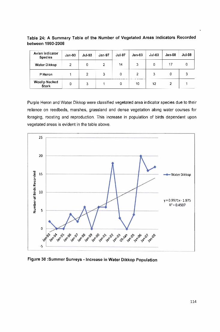
Table 24: A Summary Table of the Number of Vegetated Areas Indicators Recorded between 1993-2008
Avian Indicator Jan-93 Jul-93 Jan-97 Jul-97 Jan-03 Jul-03 Jan-OS Jul-OS
Species
Water Dikkop 2 0 2 14 3 0 17 0
P Heron 1 2 3 0 2 3 0 3
Woolly-Necked 0 3 1 0 10 12 2 1 Stork
Purple Heron and Water Dikkop were classified vegetated area indicator species due to their
reliance on reed beds, marshes, grassland and dense vegetation along water courses for
foraging , roosting and reproduction. This increase in population of birds dependent upon
vegetated areas is evident in the table above.
"C
" "C ... 0 u
" a: 11\
"C ... iii ... 0 ... " ..Q
E ::J z
25
20
15
10
5
o p,'? p,tI< p,<' p,'o p,~ p,CO p,o, S:P ~'). ~'\. ~'? ~'b<:- ~<, ~'o ~ ~q,
\1; \'b(:' \'b(:' \'b<::' \'b(:' \'b(:' \'b<::' \'b(:' \'b(:' \'b(:' \'b(:' r;:,(,} \'b(:' \'b(:' \'b(:' \'b<::'
-5
Figure 38 :Summer Surveys -Increase in Water Dikkop Population
-+-Water Dikkop
y = 0.9971x - 1.975 R2 = 0.4507
114

Plate 36: Purple Heron (Ardea purpurea)
16
14
'tl 12 qj
'tl .. 0 v
10 qj
ex: \II 'tl
8 .. iii -0 .. 6 qj .a E ::l 4 z
2
0
~ \ \ rJ\ \ I
T
\ , I \ \ I \
\ I \ .... j \ V ~ T T
Figure 39: Winter Surveys - Consistant Water Dikkop Population
...... Water Dikkop
y = 0.0088x + 4.67S R2 = SE-OS
In 1993, 1 Purple Heron and 2 Water Dikkops were observed by ornithologists. In July 2008,
Ornitholgist recored 17 Water Dikkop and 3 Purple Herons. These recordings indicate a
gradual increase in the number of sightings of particular species pointing to population
increase within the study area. This general population increase is displayed in a series of
figures displayed in the Appendix C.
115
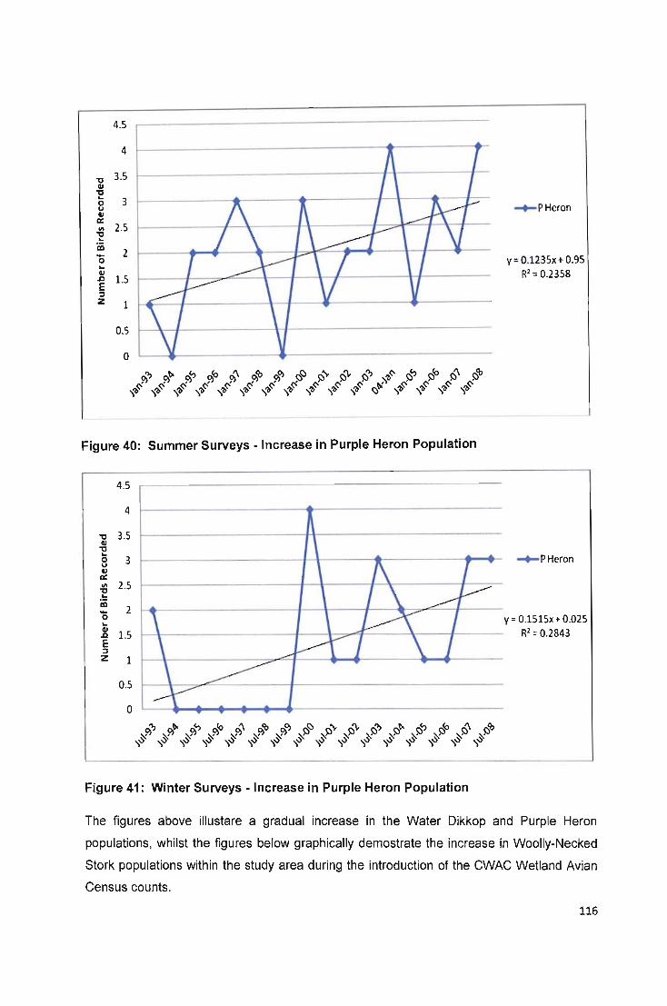
4.5
4
"0 3.5
" "0 ~
3 0 u
" ex: VI
"0 2.5
~
~ 2 -0
~
1: 1.5 E ::I Z 1
0.5
0
Figure 40: Summer Surveys - Increase in Purple Heron Population
4.5
4
"0 3.5 " "0 ~
3 0 u
" ex: II> 2.5 "0 ~
~ 2 '0
~
" 1.5 .D E ::I Z 1
0.5
0
Figure 41: Winter Surveys - Increase in Purple Heron Population
-+-PHeron
y =0.1235x+0.95 R2 = 0.2358
-+-PHeron
y = 0.1515x + 0.025 R2 = 0.2843
The figures above illustare a gradual increase in the Water Dikkop and Purple Heron
populations, whilst the figures below graphically demostrate the increase in Woolly-Necked
Stork populations within the study area during the introduction of the CWAC Wetland Avian
Census counts.
116

Plate 37: Water Dikkop (Burhinus vericulatus)
Figure 38 graphically represents the increase in the number of Water Dikkop recorded within
the study area against the time index. The figure displays a moderatly strong positive linear
with a regresssion equation of 9= 0.9971x- 1.975 and a R2= 0.4507. The number of Water
Dikkop recorded during the summer period seems to be increasing over time. The Figure 39,
also illustartes the number of birds counted plotted against the time period of the study. The
regression equation is 9= -0.0088x+4.675 with a R2=5E-05. This indicates that the Water
Dikkop population has remained constant and not flucutated signficantly over the established
time peirod.
Meanwhile, Figure 40 and 41 shows the number of Purple Herons recorded during surveys
plotted against the time index. The Figure 40 shows a regresssion equation of 9= 0.1235x +
0.95 and R2= 0.2338.This figure indicates that the population of Purple Heron is gradually
increasing during the summer months. Figure 41 displays a regression equation of 9=
0.1515x + 0.025 and R2= 0.2843. This indicates that Heron numbers are increasing over the
winter period.
Plate 38: Woolly-Necked Stork (Ciconia episcopus)
117
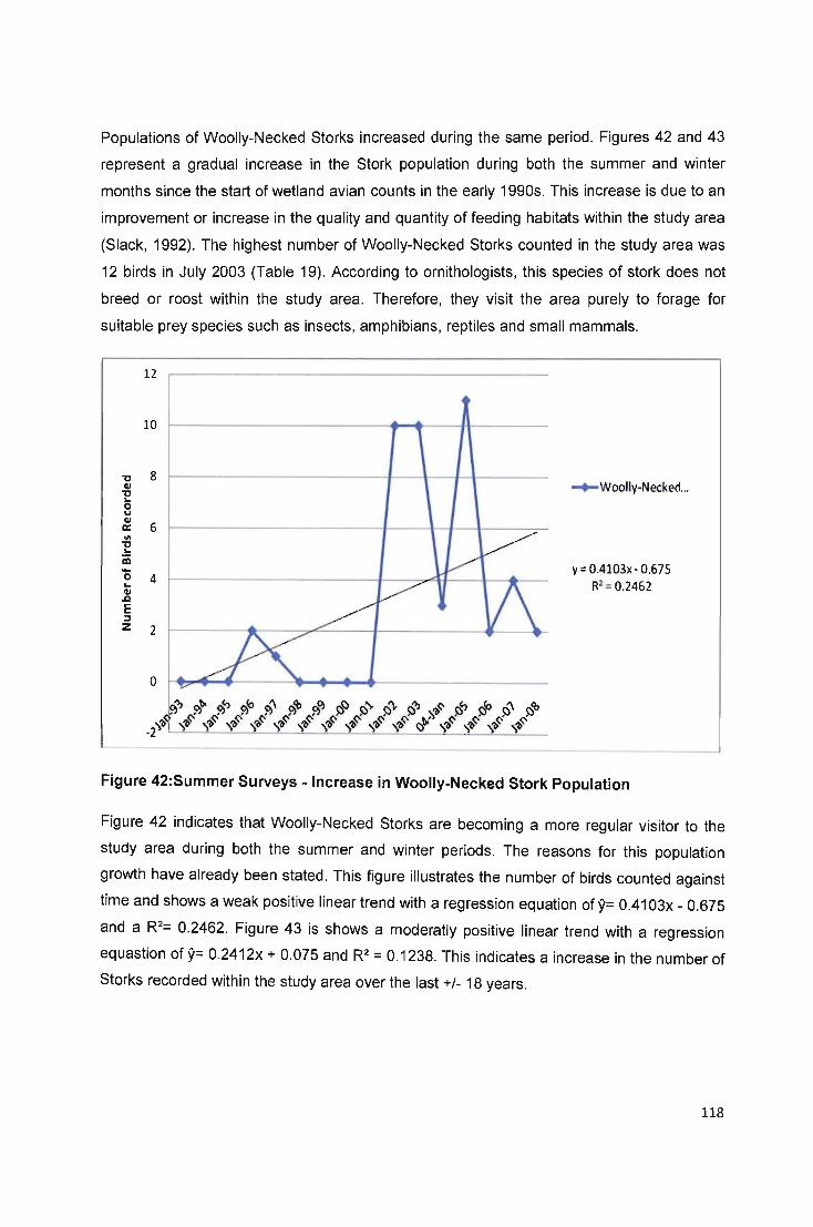
Populations of Woolly-Necked Storks increased during the same period. Figures 42 and 43
represent a gradual increase in the Stork population during both the summer and winter
months since the start of wetland avian counts in the early 1990s. This increase is due to an
improvement or increase in the quality and quantity of feeding habitats within the study area
(Slack, 1992). The highest number of Woolly-Necked Storks counted in the study area was
12 birds in July 2003 (Table 19). According to ornithologists, this species of stork does not
breed or roost within the study area. Therefore, they visit the area purely to forage for
suitable prey species such as insects, amphibians, reptiles and small mammals.
"0 CII "0 ... 0 u CII ex: lit "0 ... iii -0 ... ~ E :::I Z
12
10
8
6
4
2
0
...... Woolly-Necked ..
y = 0.4103x - 0.675 R2: 0.2462
Figure 42:Summer Surveys - Increase in Woolly-Necked Stork Population
Figure 42 indicates that Woolly-Necked Storks are becoming a more regular visitor to the
study area during both the summer and winter periods. The reasons for this population
growth have already been stated . This figure illustrates the number of birds counted against
time and shows a weak positive linear trend with a regression equation of y= 0.4103x - 0.675
and a R2= 0.2462. Figure 43 is shows a moderatly positive linear trend with a regression
equastion of y= 0.2412x + 0.075 and R2 = 0.1238. This indicates a increase in the number of
Storks recorded within the study area over the last +/- 18 years.
118
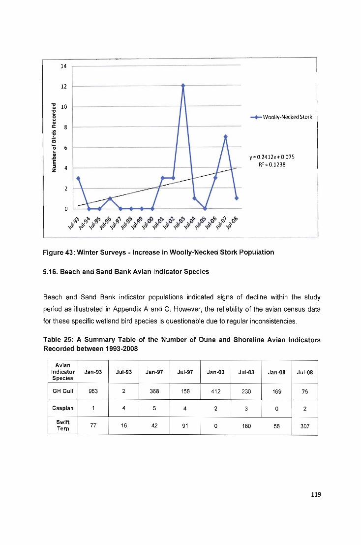
" " " .. 0 u
" ex: ell
" .. co '0 .. oX E :J z
14
12
10
8
6
4
2
0
-+-Woolly-Necked Stork
y = 0.2412x + 0.075 R2 =0.1238
Figure 43: Winter Surveys - Increase in Woolly-Necked Stork Population
5.16. Beach and Sand Bank Avian Indicator Species
Beach and Sand Bank indicator populations indicated signs of decline within the study
period as illustrated in Appendix A and C. However, the reliability of the avian census data
for these specific wetland bird species is questionable due to regular inconsistencies.
Table 25: A Summary Table of the Number of Dune and Shoreline Avian Indicators Recorded between 1993-2008
Avian Indicator Jan-93 Jul-93 Jan-97 Jul-97 Jan-03 Jul-03 Jan-OS Jul-OS Species
GHGull 963 2 368 158 412 230 169 75
Caspian 1 4 5 4 2 3 0 2
Swift 77 16 42 91 0 180 Tern 58 307
119

Figure 44 below graphically represents the number of birds recorded during the summer
periods against time. This figure indicates that there is no linear correlation between the
values. It also reveals the existence of an outlier which calls into question the reliability of the
census data for this bird species. In January 1999, a total of ten Caspian Terns were
recorded during an avian survey. The researcher had doubts about the reliability of this
avian data set, and the avian data obtained for all the bird species selected as Beach and
Sand Bank Indicators. However, as the data obtained from the Avian Demographical Unit
(UCT) was the only avain census data for the study area over consecutive years, the
researcher decided to continue the assessment with these inconsistencies and concerns in
mind.
The researcher identified a couple of reasons for the inconsistencies in the avian census
data of Swift Terns, Caspian Terns and Grey-Headed Gulls. These include:
• Firstly, confusion during the identification process by the birders leading to the
misidentification of a particular bird species. For example, another common large tern
species could be misidentified as a Caspian Tern.
• Secondly, the large numbers of birds recorded during surveys over the last two
decades calls into question the accuracy of these counts. The establishment of an
accurate number of small , active and mobile bird species such as Gulls and Terns
within a large study area is challenging. Counts of birds are often conducted over
great distances through binoculars and other viewing equipment, and determining the
exact number of bird 's present is extremely difficult.
Figure 45 represents the number of Caspian Terns recorded plotted against established time
period of the study. This figure reflects a weak negative linear trend with the regression
equation of 9= -0.2059x + 4.125 with R2 = 0.1445. The decline of Caspian Tern and Grey
Headed Gull populations is due to a decrease in the quality and quantity of roosting habitats
(beaches and sand banks. The increase in the numbers of feral cats and dogs within the
study area denies these birds access to secure roosting sights. The increase in predation by
cats on terns and gulls was confirmed during the conduction of field surveys. The researcher
witnessed feral cats catching and consuming gulls and terns on five seperate occassions
during the cause of this study. Piles of bones and scattered feathers were also found near
the beach and sand banks, abjacent to the Beachwood Mangrove Swamp Nature Reserve.
The bones and feathers were confirmed as belonging to gull and tern species by local
conservation officals (Gillard , 2008). Orithologists expressed their concern about the influx of
feral and domesticed cats into the lower esturine and mangrove ecosystem seeking food in
120
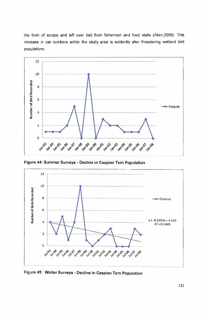
the form of scraps and left over bait from fisherman and food stalls (Allen,2008). This
increase in cat numbers within the study area is evidently also threatening wetland bird
populations.
12
10
'0 4.1 '0
8 ~
0 U 4.1
ex: '0 ~
6 iii .... 0 ~
4.1 SJ
4 E :J Z
2
0
Figure 44: Summer Surveys - Decline in Caspian Tern Population
12
10 '0 /II '0 ~
0 u
8 /II ex: ... '0 .. iii '0 6 .. /II
.Q
E ::J
4 z
2
0
-+-Caspian
-+-Caspian
v = -o.2059x + 4.125 R2 = 0 .1445
._. __ ._---------_._----_ .. _--_ .. _----_ .. _----_ .. __ .. _----------------_ .. _-.. _---_._. __ ._._--_._-------_ .. _-
Figure 45: Winter Surveys - Decline in Caspian Tern Population
121
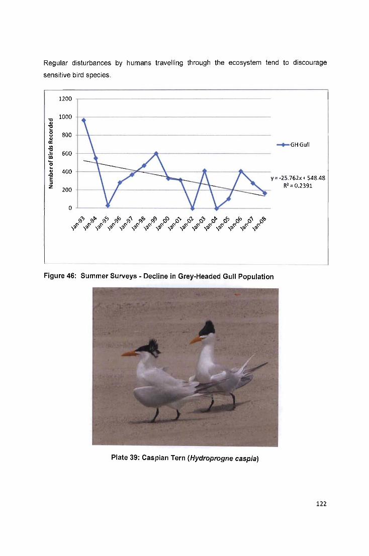
Regular disturbances by humans travelling through the ecosystem tend to discourage
sensitive bird species.
1200
"C 1000
¢I "C ... 0 800 u ¢I ex: III "C
600 .. ~ -0 .. ¢I 400 .J:! E ::J Z 200 ·
y = -25.762x+ 548.48 R2 = 0.2391
0
Figure 46: Summer Surveys - Decline in Grey-Headed Gull Population
Plate 39: Caspian Tern (Hydroprogne caspia)
122
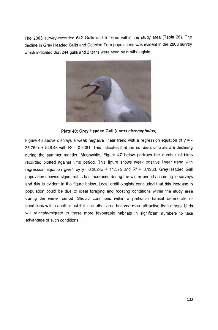
The 2003 survey recorded 642 Gulls and 5 Terns within the study area (Table 26). The
decline in Grey Headed Gulls and Caspian Tern populations was evident in the 2008 survey
which indicated that 244 gulls and 2 terns were seen by ornithologists.
Plate 40: Grey Headed Gull (Larus cirrocepha/us)
Figure 46 above displays a weak negtaive linear trend with a regression equation of 9 = -
25.762x + 548.48 with R2 = 0.2391. This indicates that the numbers of Gulls are declining
during the summer months. Meanwhile, Figure 47 below portrays the number of birds
recorded plotted against time period. This figure shows weak positive linear trend with
regression equation given by 9= 6.3824x + 11 .375 and R2 = 0.1933. Grey-Headed Gull
population showed signs that is has increased during the winter period according to surveys
and this is evident in the figure below. Local ornithologists concluded that this increase in
population could be due to ideal foraging and roosting conditions within the study area
during the winter period. Should conditions within a particular habitat deteriorate or
conditions within another habitat in another area become more attractive than others, birds
will relocate/migrate to these more favourable habitats in significant numbers to take
advantage of such conditions.
123

." CII ." ... 0 u CII a: '" ." ... iii -0 ...
CII .Q
E j
z
250
200
150
100
50
0
...... GHGull
v = 6.3824x + 11.375 R2= 0.1933
Figure 47: Winter Surveys - Increase in Grey-Headed Gull Population
Plate 41: Swift Tern (Sterna bengill
Examination of Figure C6 of Appendix C will indicate a steady increase in the Swift Tern
population within the Mgeni Estuary and Beachwood Mangrove Swamps. This increase in
the number of birds observed during the summer period in particular, is directly linked to the
increase in food supply, and an increase in the quality and quantity of foraging habiats
(Allen,2008).
Figure 48 below displays the number of Swift Terns recorded during the surveys against the
established time index. There is no linear correlation between the values in this case.
124

Inconsistencies in the number of birds recorded during surveys have contributed to this
situation and could be the result of human error.
Figure 49 indicates that there is a strong positive linear trend with a regression equation of 9 = 13.291x + 14.4 and a R2 = 0.6465. This has established that as one variable changes, the
other variable will change in a similar manner which indicates that the population of Swift
Terns is progressively increasing over the establish time period. Ornithologists counted 93
terns during 1993, and 133 in 1997. In 2003 the number of birds recorded had grown to 180
individuals. The last count in July 2008 recorded 300 terns within the study area - a dramatic
increase.
Ornithologists conclude that increased instances of disturbance caused by humans and their
pets visiting or travelling through the estuarine and mangrove ecosystem during the summer
holidays scares away waterbirds. Swift Terns are a retiring and shy tern species and
generally avoid roosting or foraging in areas frequented by fisherman , canoeist, beach-goers
and their dogs (Allen, 2008).
120
100
"l:I QI
"l:I ... 80 0 U QI a:: '" "l:I ... 60 co -0 -.-Swift Tern ... QI .c 40 E :;, z
20
0
Figure 48: Summer Surveys - Swift Tern Population
125
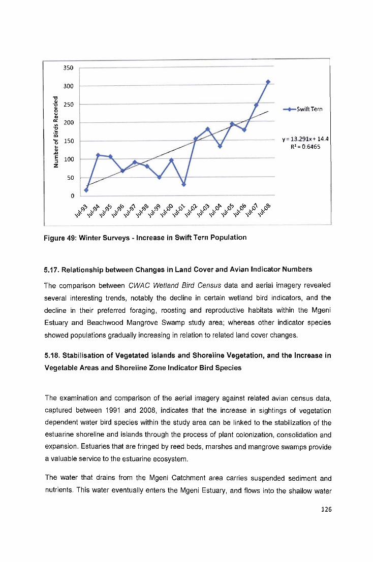
350
300
~ OJ 250 ~ .. 0
'" OJ a: 200 11\ ~ .. iii - 150 0 .. OJ
.Q
E 100 :::I Z
50
a
Figure 49: Winter Surveys - Increase in Swift Tern Population
-.-SwiftTern
y = 13.291x + 14.4 R2 = 0.6465
5.17. Relationship between Changes in Land Cover and Avian Indicator Numbers
The comparison between CWAC Wetland Bird Census data and aerial imagery revealed
several interesting trends, notably the decline in certain wetland bird indicators, and the
decline in their preferred foraging, roosting and reproductive habitats within the Mgeni
Estuary and Beachwood Mangrove Swamp study area; whereas other indicator species
showed populations gradually increasing in relation to related land cover changes.
5.18. Stabilisation of Vegetated Islands and Shoreline Vegetation, and the Increase in
Vegetable Areas and Shoreline Zone Indicator Bird Species
The examination and comparison of the aerial imagery against related avian census data,
captured between 1991 and 2008, indicates that the increase in sightings of vegetation
dependent water bird species within the study area can be linked to the stabilization of the
estuarine shoreline and islands through the process of plant colonization, consolidation and
expansion . Estuaries that are fringed by reed beds, marshes and mangrove swamps provide
a valuable service to the estuarine ecosystem.
The water that drains from the Mgeni Catchment area carries suspended sediment and
nutrients. This water eventually enters the Mgeni Estuary, and flows into the shallow water
126

channels that dissect the chain of estuarine islands. The flat estuary is characterised by a
lowering of the water velocity, and help reeds, grasses, sedges and mangrove tree clusters
take root and filter out nutrients and sedjment from the water (Gillard, 2008). Scientists
indicate that mangrove tree roots assist in the removal of sediment and help protect the
islands from water erosion and scouring flood waters. Mangrove vegetation helps stabilise
the islands and allows other vegetation with shallower root systems to become established.
Over time, the deposition of sediment decreases the depth of the river channels around the
islands, forming new mudflats which are eventually colonized by reeds, sedge and grass
species that in turn help prevent further erosion by stabilizing the growing shoreline (Garland
and Moleko, 2000). This concept will be discussed in more detail later in this chapter.
Plates 44 and 48 graphically illustrate the land cover changes that have occurred within the
Mgeni Estuary and Beachwood Swamp study area between 1991 and 2008. The
comparative plates represent these changes in land cover increases or decreases, relative
to the precise location of the 1991 land cover 'core' - the basis against which all land cover
change can be measured. For example, the core of the mangrove forest is represented in
pale green, whereas an area where the mangrove swamp has increased or decreased is
represented by light green and red respectively. This method of mapping was developed to
graphically represent significant changes in various land cover types during the study period.
When such data is compared against avian census data, it is possible to correlate and
interpret indicator bird population changes against related land cover trends during the study
period.
Plate 42: Mangrove Seedlings, Reeds and Grass Species on Island in the Mgeni
Estuary
127

Island mangrove vegetation, reed beds, marshes and grasslands have all managed to
successfully colonize, consolidate and expand their area coverage of the islands and
estuarine shoreline along a significant portion of the Mgeni Estuary as seen in Figure 41 . In
1991 , Reed Beds and Grassland habitats covered 4.51 ha (2.8%) of the study area.
However, by 2008 it covered 9.6 ha (6.0%) of the study area which is an increase in total
land coverage of 4.8%. Reed Bed and Marsh habitats covered an estimated 10.64 ha (6.7%)
of the study area in 1991. However, as reed beds and marshes progressively reverted to
reed beds with mixed sedge and grass species, the area covered by this land cover type
decreased to 9.60 ha (6.4%) of the study area.
Established vegetation also showed signs of densification. The increase in vegetation cover
represented by the reed beds, grasslands and mangrove clusters on estuarine islands and
along estuary shore lines, have all combined to create an ideal habitat for wetland bird
species that primarily rely upon reed beds, marshes and other vegetated covers for roosting,
foraging and procreation. This makes the Mgeni Estuary and adjacent Beachwood
Mangrove Swamps study area an ideal habitat for skulking bird species such as Purple
Heron and Water Dikkop (See Appendix F). These species spend much of their lives in
structurally complex habitats such as reed beds, marshes and mangrove clusters that make
locating and identifying them during census conditions challenging .
The Purple Heron is seldom seen because it tends to favour dense vegetation close to the
water's edge, and prefers to forage within this habitat or along the channels and waterways
flowing through such vegetation . The Purple Heron is rarely seen foraging for its prey out in
the open like other heron species. Ornithologists mention that this species is particularly fond
of Phragmites Reed beds found in abundance along the estuarine shoreline and island
networks. Conversely, the Water Dikkop is a common nocturnal wetland bird species that is
found along the banks of large rivers, lakes, dams, estuaries and lagoons where there is a
dense fringe of vegetation . Water Dikkop can be found lying up during the day in reed beds,
or underneath overhanging bushes, trees and other vegetation along the water's edge.
Examination of the avian census data indicated that numbers of Water Dikkop, Purple Heron
and Woolly-Necked Storks (skulking bird species) observed and recorded within the Mgeni
Estuary and Beachwood Mangrove Swamp had increased steadily between 1993 and 2008.
The increase in the populations of these 3 species, strongly correlate to the noted increase
in related vegetation cover on the estuary islands and shorelines.
Figures 50 below shows the number of Purple Herons recorded plotted against the area
covered by reed beds, marshes and grassland land cover classes within the study area. It is
128

obvious from examining the figure below that the Purple Heron numbers within the study
area have remained relatively stable between 1991 and 2008. This indicates that the
population of Purple Heron has not been positively or negatively affected by the increase in
the area coverage of reed beds, marshes and grassland land cover classes within the study
area.
Figure 51 graphically represents the number of Woolly-Necked Storks recorded within the
study area plotted against the changes in the total area covered by reed beds, marshes and
grassland land cover classes. The figure indicates a correlation coefficient of 0, thus
changes in the variables are also random and unpredictable. Therefore, it is difficult to
establish an indisputable link between changes in the area coverage of the land cover
classes and the fluctuation in this avian indicator population.
"0 6
Q) "0 .. 5 0 (,) Q)
a:: 4 c:
0 .. Q)
::J: 3 Q)
Q. .. 2 ::::s
~ ... 0
1 .. Q)
.t'l E
0 ::::s Z
• P Heron
0 5 10 15 20 25
Total Area Covered by Reed Beds, Marshes and Grassland Land Cover Classes (Ha)
Figure 50: Correlation between Land Cover Change and Fluctuations in Purple Heron
Populations
129
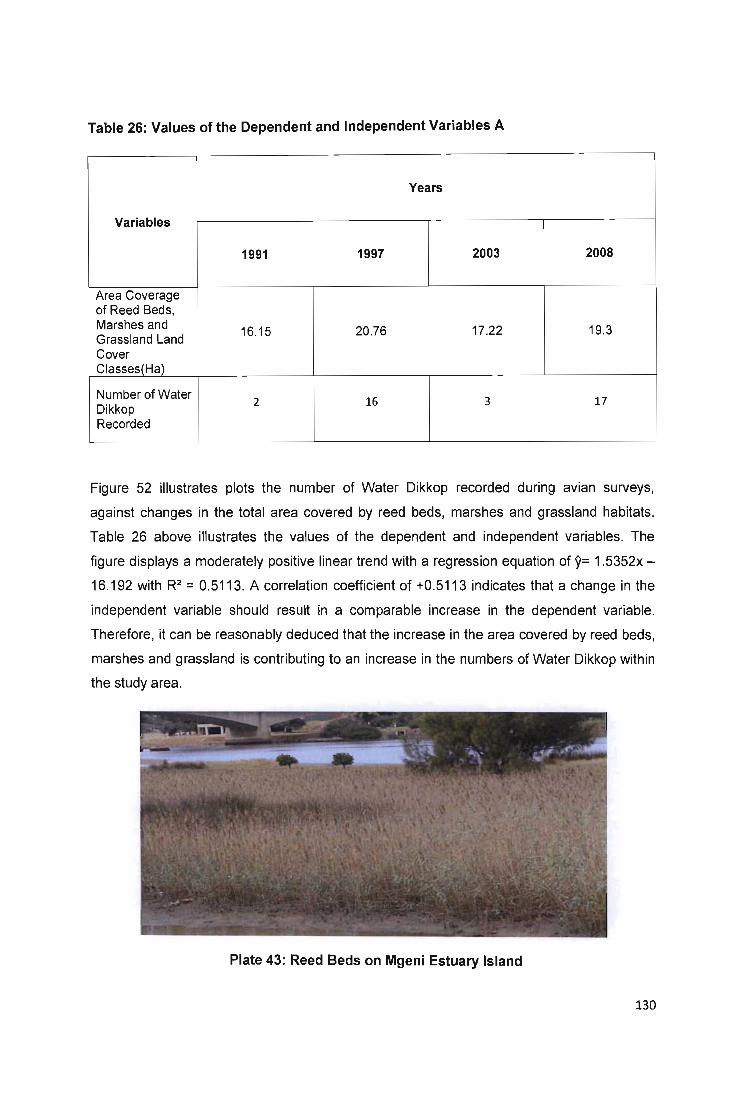
Table 26: Values of the Dependent and Independent Variables A
Years
Variables
1991 1997 2003 2008
Area Coverage of Reed Beds, Marshes and 16.15 20.76 17.22 19.3 Grassland Land Cover Classes(Ha)
Number of Water 2 16 3 17
Dikkop Recorded
Figure 52 illustrates plots the number of Water Dikkop recorded during avian surveys,
against changes in the total area covered by reed beds, marshes and grassland habitats.
Table 26 above illustrates the values of the dependent and independent variables. The
figure displays a moderately positive linear trend with a regression equation of y= 1.5352x-
16.192 with R2 = 0.5113. A correlation coefficient of +0.5113 indicates that a change in the
independent variable should result in a comparable increase in the dependent variable.
Therefore, it can be reasonably deduced that the increase in the area covered by reed beds,
marshes and grassland is contributing to an increase in the numbers of Water Dikkop within
the study area.
Plate 43: Reed Beds on Mgeni Estuary Island
130
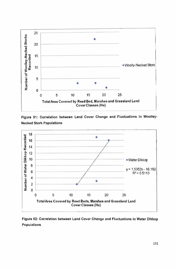
25 fI) .¥ ~
0 Q) 20 ."
CD .¥ (,)
CD." 15 ZCD '." :>.~
.!o -(,) o CD 10 00:: ;: '0 ~ 5 CD .c E :::J
Z 0 0
•
• Woolly-Necked Stork
• • • 5 10 15 20 25
Total Area Covered by Reed Bed, Marshes and Grassland Land Cover Classes (Ha)
Figure 51: Correlation between Land Cover Change and Fluctuations in Woolley
Necked Stork Populations
." 18 CD ." 16 ~
0 (,)
14 CD 0::
g. 12 .¥
~ 10 c ~
8 CD ... ('CI
;: 6 ... 0 4 ~
CD .c 2 E
:::J Z 0
o
/ /
/ '"
5 10 15
• ....
/ L
/ /
• 20 25
• Water Dikkop
y= 1.5352x-16.192 R2 = 0.5113
Total Area Covered by Reed Beds, Marshes and Grassland Land Cover Classes (Ha)
Figure 52: Correlation between Land Cover Change and Fluctuations in Water Dikkop
Populations
131

In conclusion, the findings of this study indicate that Purple Heron population remained
relatively constant and unaffected by the changes in the area coverage of reed beds,
marshes and grassland land cover classes. In addition, fluctuations in the population of
Woolley-Necked Storks cannot be indisputably linked to the changes in the area coverage of
the land cover classes. However, evidence suggests that fluctuations in the Water Dikkop
population were strongly linked to changes in the area covered by vegetated area land cover
classes. This indicates that Water Dikkop are ideal reed bed, marsh and grassland indicator
species.
5.19. Decline in Grassland and Scrub Land Cover Class
The grassland and scrub land cover class is showing signs of decline. As already noted, in
1991 this land cover class covered approximately 13.21 ha of the study area. This shrunk to
just 3.52 ha by 2008. This decline is attributed to the expansion of woodland and coastal
forest land cover classes into areas previous designated as grassland and scrub due to the
absence of a regular fire regime and logging within the study area.
Table 27: Values of Dependent and Independent Variable B
Years
Variables
1991 1997 2003 2008
Area Coverage
of Grassland and
Scrub Land 13.21 11.51 3.47 3.52 Cover Class
(Ha)
Area Coverage
of Coastal Forest
Land Cover 7.12 5.69 14.07 14.06
Class (Ha)
Area Coverage
of Woodland
Land Cover 4.69 4.19 10.91 8.26
Class (Ha)
132

Figures 53 and 54 below illustrate changes in the total area of grassland and scrub plotted
against changes in the total areas covered by woodland and coastal forest. Table 27
displays the values of the dependent and independent variables used to generate the figures
below. Figure 53 displays a strong negative linear trend with a regression equation of y = -
1.1171 x + 19.361 and R2 = 0.9309. This reveals that as coastal forest expands, grassland
and scrub areas will decline.
Figure 54 plots changes in the total area covered by grassland and scrub land cover class
against the changes in total area covered by woodland land cover class. The figure reveals a
strong negative linear trend with an equation of y = -1 .503x + 18.467 and R2 = 0.8498. This
figure illustrates a similar relationship as Figure 53, where the expansion of woodland areas
within the study area is actually having a negative impact upon grassland and scrub habitats.
14 ,,-c:(U (U:r:
12 --I/ll/l I/ll/l (U(U ... - 10 C)u >.'" .Q~
8 "0 ~U
~" 6 oC: uj (U.Q 4 C1>:J ...... «u -(I)
2 ~" oc: t-(U
o o
", .
• ~ ~ ~
5 10
.~ '+
15
• Grassland and Scrub Land Cover Class
y=-1 .1171x + 19.361 R2= 0.9309
Total Area Covered by Coastal Forest Land Cover Class (Ha)
Figure 53: Illustrating Relationship between Changes in Land Cover Classes within
Study Area (1991-2003)
133
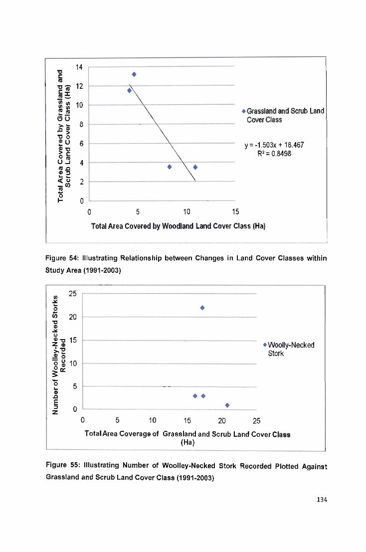
o
+ +\
\ \
\ +
5
~
10 15
• Grassland and Scrub Land Cover Class
y = ·1.503x + 18.467 R2= 0.8498
Total Area Covered by Woodland Land Cover Class (Ha)
Figure 54: Illustrating Relationship between Changes in Land Cover Classes within
Study Area (1991-2003)
... Q)
.Q E ::J Z o
o
+
•• • 5 10 15 20 25
• Woolly-Necked stork
Total Area Coverage of Grassland and Scrub Land Cover Class (Ha)
Figure 55: Illustrating Number of Woolley-Necked Stork Recorded Plotted Against
Grassland and Scrub Land Cover Class (1991-2003)
134

Woolley-Necked Storks and Water Dikkop can often be observed in Grassland and Scrub
habitats during visits to the Mgeni Estuary and Beachwood Mangrove Swamps. Storks and
Dikkops tend to forage in open grass areas.
Figure 55 shows the number of Woolley-Necked Storks recorded plotted against the total
area covered by the grassland and scrub land cover class. A correlation coefficient of 0
indicates that the changes that occur in the independent and dependent variables are
random and unrelated. There is no relationship between the variables and thus no linear
correlation.
Therefore, despite the decline in the area covered by grassland and scrub, Woolley-Necked
Stork numbers are gradually increasing within the study area in which they do not roost and
breed . This species simply visits vegetated areas within the study area because they are
ideal foraging locations (See Appendix F). Therefore, land cover change within the study
area would not have an impact on their population because of their ability to move freely
between a wide variety of different land cover classes and sub-classes found in other
grassland, riverine, estuarine and wetland ecosystems scattered throughout the greater
eThekweni area. This suggests that this bird species is not a good indicator species.
18
• 'a 16 ..... QI 'a ... 14 0 u QI
cc: 12 Q. 0 ~ ~ 10 0 ... QI 8 .. • Water Dikkop
IV
~ 6 -0 ...
.B 4 E = • z 2 .....
a 0.00 2.00 4.00 6.00 8.00 10.00 12.00 14.00
Total Area Covered by l and Cover Classes
Figure 56: Illustrating Number of Water Dikkop Recorded Plotted Against Grassland
and Scrub Land Cover Class (1991-2003)
135
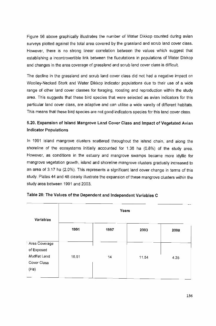
Figure 56 above graphically illustrates the number of Water Dikkop counted during avian
surveys plotted against the total area covered by the grassland and scrub land cover class.
However, there is no strong linear correlation between the values which suggest that
establishing a incontrovertible link between the flucutations in populations of Water Dikkop
and changes in the area coverage of grassland and scrub land cover class is difficult.
The decline in the grassland and scrub land cover class did not had a negative impact on
Woolley-Necked Stork and Water Dikkop indicator populations due to their use of a wide
range of other land cover classes for foraging, roosting and reproduction within the study
area. This suggests that these bird species that were selected as avian indicators for this
particular land cover class, are adaptive and can utilise a wide vareity of different habitats.
This means that these bird species are not good indicators species for this land cover class.
5.20. Expansion of Island Mangrove Land Cover Class and Impact of Vegetated Avian
Indicator Populations
In 1991 island mangrove clusters scattered throughout the island chain, and along the
shoreline of the ecosystems initially accounted for 1.38 ha (0.8%) of the study area.
However, as conditions in the estuary and mangrove swamps became more idyllic for
mangrove vegetation growth, island and shoreline mangrove clusters gradually increased to
an area of 3.17 ha (2.0%). This represents a significant land cover change in terms of this
study. Plates 44 and 48 clearly illustrate the expansion of these mangrove clusters within the
study area between 1991 and 2003.
Table 28: The Values of the Dependent and Independent Variables C
Years
Variables
1991 1997 2003 2008
Area Coverage
of Exposed
Mudflat Land 16.51 14 11.54 4.25 Cover Class
(Ha)
136
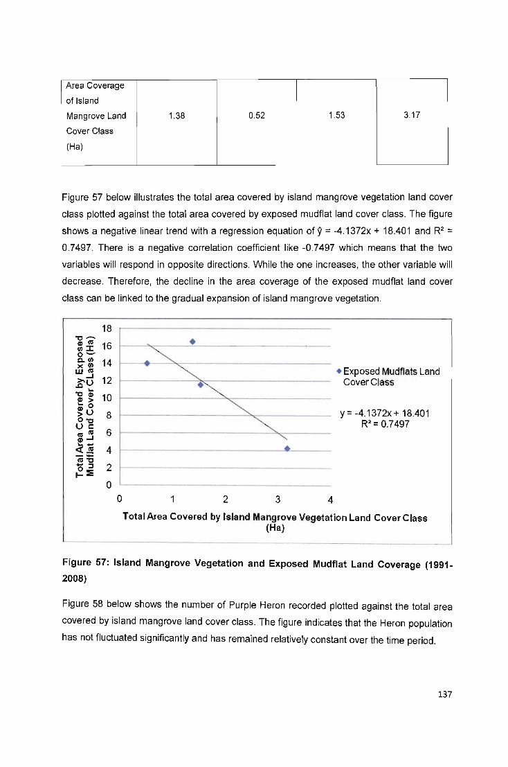
Area Coverage
of Island
Mangrove Land 1.38 0.52 1.53 3.17
Cover Class
(Ha)
Figure 57 below illustrates the total area covered by island mangrove vegetation land cover
class plotted against the total area covered by exposed mudflat land cover class. The figure
shows a negative linear trend with a regression equation of y = -4.1372x + 18.401 and R2 = 0.7497. There is a negative correlation coefficient like -0.7497 which means that the two
variables will respond in opposite directions. While the one increases, the other variable will
decrease. Therefore, the decline in the area coverage of the exposed mudflat land cover
class can be linked to the gradual expansion of island mangrove vegetation.
18 "0 -Q) to 16 (I):I: 0-Q.(I) x (I) 14 wto >-..J 12 ,gu ...
"OQ) 10 Q) > ... 0 ~U 8 0"0 Uc:
6 to to Q)..J ..... c:(~ 4 --to "0 0::::1 t-:E 2
0
o
• ~ ~
.~
~
1 2
~ "-•
3 4
• Exposed Mudflats Land Cover Class
y= -4.1372x+ 18.401 R2= 0.7497
Total Area Covered by Island Mangrove Vegetation Land Cover Class (Ha)
Figure 57: Island Mangrove Vegetation and Exposed Mudflat Land Coverage (1991-
2008)
Figure 58 below shows the number of Purple Heron recorded plotted against the total area
covered by island mangrove land cover class. The figure indicates that the Heron population
has not fluctuated significantly and has remained relatively constant over the time period.
137
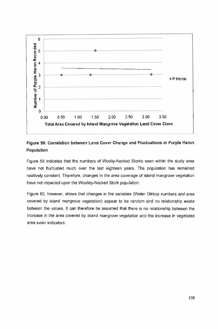
't' CD
6
'E5 o (,) CD
0::: c4 o ... CD ::I: CD3 Q. ... ::l 0-2 '0 ... CD
~ 1 ::l Z
o
.... + P Heron
0.00 0.50 1.00 1.50 2.00 2.50 3.00 3.50
Total Area Covered by Island Mangrove VegetatIon Land Cover Class
Figure 58: Correlation between Land Cover Change and Fluctuations in Purple Heron
Population
Figure 59 indicates that the numbers of Woolly-Necked Storks seen within the study area
have not fluctuated much over the last eighteen years. The population has remained
relatively constant. Therefore, changes in the area coverage of island mangrove vegetation
have not impacted upon the Woolley-Necked Stork population.
Figure 60, however, shows that changes in the variables (Water Dikkop numbers and area
covered by island mangrove vegetation) appear to be random and no relationship exists
between the values. It can therefore be assumed that there is no relationship between the
increase in the area covered by island mangrove vegetation and the increase in vegetated
area avian indicators.
138

", .:.:. .. 0 ... en "0
CD .¥ u
CD "0 ZCD '''0 >- ..
.!!o -u o CD 00:: 3: -0 ..
CD ..c E :::J
Z
25
• 20
15 • Woolly-Necked Stork
10 Y = -0.014x + 7.273
R2 = 2E-06 5
• • 0 • 0.00 1.00 2.00 3.00 4.00
Total Area Covered by Island Mangrove Vegetation Land Cover Class (Ha)
Figure 59: Correlation between Land Cover Change and Fluctuations in Woolley
Necked Stork Population
"0 CD 'tI .. 0 u CD
0:: Q. 0
.:.:.
.¥
C .. CD ... tU
3: -0 .. II> .c E :::J Z
18
• 16 ..... T
14
12
10
8 • Water Dikkop
6
4
• 2
o 0.00 0.50 1.00 1.50 2.00 2.50 3.00 3.50
Total Area Covered by Island Mangrove Vegetation Land Cover Class (Ha)
------ ------- -- ------- ------ -------------------------- --- --._-_ .. - .... _-._ ... -... ----_ ... - _ .. _---_ .. _-----'
Figure 60: Correlation between Land Cover Change and Fluctuations in Water Dikkop
Population
139

In conclusion, the expansion of mangrove vegetation is having a detrimental impact on the
mudflat land cover class throughout the lower part of the Mgeni Estuary. The increase in the
area covered by mangrove vegetation is clealry evident in Plates 43 and 46. Figure 57
graphically illustartes the decline of exposed mudflats due to the colonisation and expansion
of mangrove vegetaion through the chain of isalnds and mudflats scattered throught the
estuary. Further research found that Purple Heron and Woolley-Necked Stork numbers
remain relatively stable and consistent throughout the study period, whilst the area covered
by island mangrove vegetation expanded resulting in a decline in exposed mudlfats. This
indicates that these avian indicator species were uneffected by the changes in land cover.ln
addition, the study was unable to provide indistuptable evidence to argue that there is a link
between the increase in Water Dikkop populations and the increase in area coverage of
island mangrove vegetation. Ornithologists and local conseration officals argue that the
increase in the numbers of Water Dikkop within the study area could be a seasonal
phenomenon.
5.21. Reduction in Sediment, and the Subsequent Impact on Mudflat, Dune and Shoreline Avian Indicators
The researcher concluded that the decrease in the total area covered by mudflats, beaches
and sandbanks within the study area could be due to two factors. Firstly, several studies
relating to the annual sediment yield of the Mgeni River were examined. The studies noted
that the sediment yield of the river was approximately 1-6x 10* tonnes (Garland and Moleko,
2000). However, the construction of five dams within the catchment area has drastically
reduced the contemporary sediment yield to the coast. The catchments area below the four
main dams that were completed prior to 1987 is estimated to be around 1700 Km2, and the
total sediment yield from this area was calculated to be around 0-5 x 10* tonnes per year
(Garland and Moleko, 2000).
The completion of the Inanda Dam in 1988 has only exacerbated the situation by altering
bed load transportation and deposition. After the completion of the Inanda Dam, the mean
annual discharge of the river was Significantly reduced (4%). The establishment of a water
release policy also had a major impact on the discharge regime which has led to an increase
in competent discharge events (Gillard, 2008). Sediment continually builds up behind the
dam wall, which has led to a notable reduction in available downstream sediment. Whereas
the volume of sediment within the estuary has not changed since 1989, the sediment calibre
has become much finer (McCally, 2007).
140
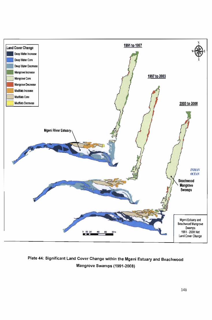
Land Cover Change
• Deep Water Increase
Deep Water Core
Deep Water Decrease
Mangrove Increase
Mangrove Core
• Mangrove Decrease
• Mudflats Increase
D Mudflats Core
Mudflats Decrease
Mgeni River Estuary
o 100 200 «10 tm tmm MM
1991 to 1997
1997 to 2003
2003 to 2008
INDIAN OCEA,'"
Mgeni Estuary and Beachwood Mangrove
Swamps 1991 - 2008 Net
Land Cover Change
Plate 44: Significant Land Cover Change within the Mgeni Estuary and Beachwood
Mangrove Swamps (1991-2008)
141
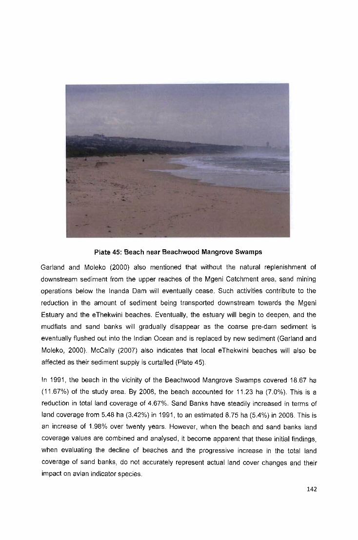
Plate 45: Beach near Beachwood Mangrove Swamps
Garland and Moleko (2000) also mentioned that without the natural replenishment of
downstream sediment from the upper reaches of the Mgeni Catchment area, sand mining
operations below the Inanda Dam will eventually cease. Such activities contribute to the
reduction in the amount of sediment being transported downstream towards the Mgeni
Estuary and the eThekwini beaches. Eventually, the estuary will begin to deepen, and the
mudflats and sand banks will gradually disappear as the coarse pre-dam sediment is
eventually flushed out into the Indian Ocean and is replaced by new sediment (Garland and
Moleko, 2000). McCally (2007) also indicates that local eThekwini beaches will also be
affected as their sediment supply is curtailed (Plate 45).
In 1991, the beach in the vicinity of the Beachwood Mangrove Swamps covered 18.67 ha
(11.67%) of the study area. By 2008, the beach accounted for 11 .23 ha (7.0%). This is a
reduction in total land coverage of 4.67%. Sand Banks have steadily increased in terms of
land coverage from 5.48 ha (3.42%) in 1991, to an estimated 8.75 ha (5.4%) in 2008. This is
an increase of 1.98% over twenty years. However, when the beach and sand banks land
coverage values are combined and analysed , it become apparent that these initial findings,
when evaluating the decline of beaches and the progressive increase in the total land
coverage of sand banks, do not accurately represent actual land cover changes and their
impact on avian indicator species.
142

Table 29: The Values of Dependent and Independent Variables D
Years
Variables
1991 1997 2003 2008
Area Coverage
of Exposed
Mudflat Land 16.51 14 11.54 4.25
Cover Class
(Ha)
Number of
Beach and
Sandbank Avian 1063 668 827 611
Indicators
Recorded
Table 29 presents the values of the variables used in this Figure 61. This figure indicates
that the beach and sand banks are declining slightly in terms of their total land coverage
within the study area, and the dune and shoreline avian indicator species numbers also
show a decline in population numbers, all of which is illustrated by the trend line in the graph
below. This suggests a possible relationship between changes in area coverage of the land
cover classes and the fluctuations in avian indicator populations.
The decline in the population of Caspian Terns and Grey Headed Gulls can be the result of a
decrease in the quality and quantity of their preferred roosting habitats in the form of sand
banks and beaches within the Mgeni Estuary and Beachwood Mangrove Swamp ecosystem.
This could possibly be attributed to greater access by land-based predators (cats and dogs)
to such beach locations as already stated (See Append ix F). The beaches in the vicinity of
the study area are used for recreational purposes such as fishing , canoeing and walking .
Such regular disturbances by humans travelling through the sensitive ecosystem may have
resulted in indicator species moving away to undisturbed locations (Kalejta and Hockey,
1991).
143

I: 1200 III '5 c( 1000 ~ I: 111"0 ala> 800 "0"0 1:'" 1110 tn U
a> 600 "00:::
1:1/1 III ... J:,O u1U 400 IIIu a>_ al"O .... 1: 0- 200 ... a> .Q
E 0 :::s z
• . / ~.
• Beach and Sand Bank Avian Indicator Population
1------------------ Y = 43.836x - 96.968 R2= 0.403
0 5 10 15 20 25 30
Total Area Covered by Beach and Sand Bank Land Cover Classes (Ha)
Figure 61: Number of Beach and Sand Bank Avian Indicators Recorded plotted
against Total Area Covered by Beach and Sand Bank Land Cover Classes (1991-2008)
Figure 62 graphically represents the number of beach and sand bank avian indicators
plotted against the total area covered by beach and sand bank land cover classes between
1991 and 2008. The figure has a moderately strong positive linear trend with a regression
equation of y = 43.836x - 96.968 and R2 = 0.403. This illustrates that there is indeed a
possible relationship between the decline in the land cover classes and populations of avian
indicators.
The figures below seek to determine if there is a link between the changes in these land
cover classes and fluctuations of avian indicator species. Figure 62 displays the number of
Caspian Terns recorded plotted against the total area covered by beach and sand bank land
cover classes within the study area. However, the figure shows that the variables are
random and there is no relationship between them, which means there is no linear
correlation.
144
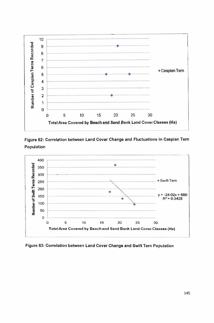
10 " Q)
9 " """'-T ...
0 8 (,)
Q)
0:: 7 (/) c ... 6 Q)
~ c 5 «I
..... T
• Caspian Tern
"a. 4 (/)
«I 0 3 -0 ... 2 Q) ..c E 1 :::s z
0
o 5 10 15 20 25 30
Total Area Covered by Beach and Sand Bank Land Cover Classes (Ha)
Figure 62: Correlation between Land Cover Change and Fluctuations in Caspian Tern
Population
400 "C Q)
350 "C ... 0 Co)
300 Q)
0:: til 250 c: ... Q) .... 200 l U) 150 -0 ... 100 Q) .c E 50 :::J
Z 0
o
"-
•
5 10 15
•
~ ~ . ~
•
20 25
+ SWift Tern
30
y = -24.02x + 680 R2= 0.3428
Total Area Covered by Beach and Sand Bank Land Cover Classes (Ha)
Figure 63: Correlation between Land Cover Change and Swift Tern Population
145

Table 30: The Values of the Dependent and Independent Variables E
Years
Variables
1991 1997 2003 2008
Area Coverage
of Beach and
Sand Bank 24.13 20.8 17.33 19.98
Land Cover
Classes(Ha)
Number of
Grey-Headed 965 526 642 224
Gull Recorded
Number of
Swift Tern 93 133 180 365
Recorded
The table above shows the values of the dependent and independent values used to create
the following figures. Figure 63 represents the number of Swift Terns recorded plotted
against changes in the total area of the beach and sand bank land cover classes. This figure
displays a weak negative linear trend. The regression equation for this figure is y = -24.02x +
680 and the R2 = 0.3428. Therefore changes in one variable are reflected by changes in the
second variable in the other direction. Therefore, the decline in Beaches and Sand Bank
habitats is not having a negative impact on Swift Tern populations. In fact, Swift Tern
numbers are increasing in the study area.
Figure 64 represents the number of Grey-Headed Gulls plotted against changes in the total
area of the beach and sand bank land cover classes. The figure displays a positive linear
trend with a regression equation of y = 67 .613x - 777.27 and R2 = 0.4409. This means that
changes in the one variable result in similar changes in the other variable. The positive
correlation between its variables, which indicates that there is a possible relationship
between the decline in Grey-Headed Gull populations and the decline in these land cover
classes within the Mgeni Estuary and Beachwood Mangrove Swamp study area. This
146

indicates that there is a possible relationship between the decline in the area covered by
beach and sand bank land cover classes and the decline in avian indicator species.
1200
~ '3 1000 C) + "
+ / +GHGull
CD
" 800 tV" CD CD :1:" I ...
600 >-0 ! () C)CD .... 0:::
400 0 ...
/
/+
I----------~ _______ y = 67.613x - 777.27 R2 = 0.4409
CD .c E 200 :::J
+ Z
0
0 5 10 15 20 25 30
Total Area Covered by Beach and Sand Bank Land Cover Classes (Ha)
Figure 64: Correlation between Land Cover Change and Fluctuations in Grey-Headed
Gull Population
In conclusion, on closer examination of the figures, it has been determined that there is
some degree of correlation between changes in these beach and sand bank land cover
classes and the fluctuations in the populations of Gull and Tern species. This is despite
inconsistencies and irregularities in the avian census data used to produce these findings .
For example, there is a moderately strong correlation between the decline in the Grey
Headed Gull population and the decline in the area coverage of beach and sand bank land
cover classes between 1991 and 2008.
5.22. Mangrove Vegetation Expansion and the Decline of Mudflat Habitats and Avian Indicators
Another factor contributing to the steady disappearance of the mudflats is the following:
Closer examination of the mudflats and islands in aerial imagery, taken of the Mgeni Estuary
and Beachwood Mangrove Swamp study area over the last two decades, has revealed the
progressive expansion of the mangrove community into the estuary and the lower reaches of
river estuarine ecosystem as seen in Plate 44 and 48 (Gillard, 2008).
147
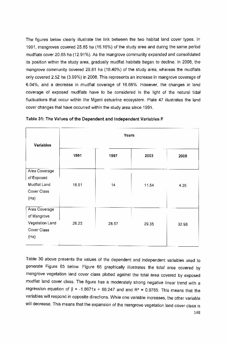
The figures below clearly illustrate the link between the two habitat land cover types. In
1991, mangroves covered 25.85 ha (16.16%) of the study area and during the same period
mudflats cover 20.65 ha (12.91 %). As the mangrove community expanded and consolidated
its position within the study area, gradually mudflat habitats began to decline. In 2008, the
mangrove community covered 29.81 ha (18.40%) of the study area, whereas the mudflats
only covered 2.52 ha (3.99%) in 2008. This represents an increase in mangrove coverage of
6.04%, and a decrease in mudflat coverage of 16.66%. However, the changes in land
coverage of exposed mudflats have to be considered in the light of the natural tidal
fluctuations that occur within the Mgeni estuarine ecosystem. Plate 47 illustrates the land
cover changes that have occurred within the study area since 1991 .
Table 31: The Values of the Dependent and Independent Variables F
Years
Variables
1991 1997 2003 2008
Area Coverage
of Exposed
Mudflat Land 16.51 14 11.54 4.25
Cover Class
(Ha)
Area Coverage
of Mangrove
Vegetation Land 26.23 28.57 29.35 32.98
Cover Class
(Ha)
Table 30 above presents the values of the dependent and independent variables used to
generate Figure 65 below. Figure 65 graphically illustrates the total area covered by
mangrove vegetation land cover class plotted against the total area covered by exposed
mudflat land cover class. The figure has a moderately strong negative linear trend with a
regression equation of 9 = -1.8671x + 66.247 and and R2 = 0.9765. This means that the
variables will respond in opposite directions. While one variable increases, the other variable
will decrease. This means that the expansion of the mangrove vegetation land cover class is
148

causing a reduction in the area coverage of the exposed mudflat land cover class within the
study area.
Tidal fluctuation assists in the dispersal of seeds from the Beachwood Mangrove Swamp
Nature Reserve which has allowed Avicennia germinans (Black Mangrove) and Laguncu/aria
racemosa (white mangrove) to spread and be established within the lower estuarine and
river ecosystems. This has led to a gradual disappearance of the mudflat habitat within the
lower estuarine and river ecosystem as seen in Plates 44 and 48. As a result, wading bird
populations (mudflat avian indicator species) have steadily declined because of their reliance
on these habitat systems (Gillard, 2008).
20 ,,-Q)IV 18 Cl)J: 0-
16 CaCl) XCI) WIV 14 >..J ,cU
12 " ... Q)Q) ... > 10 Q)o >U 0" Uc 8 IV IV Q).J 6 ..... ~IV 4 -~ IV" "::I ~::E 2
0 o
• \. \ } S \ i
10 20 30 40
• Exposed Mudflat Land Cover Class (Ha)
y=-1.8671x + 66.247 R2= 0.9765
Total Area Covered by Mangrove Vegetation Land Cover Classes (Ha)
Figure 65: Mangrove Vegetation and Exposed Mudflat Land Coverage (1991-2008)
The Avicennia germinans (Black Mangrove) and Laguncu/aria racemosa (White Mangrove)
species are pioneering plants that colonize muddy and sandy banks of estuaries and other
inlets. As mentioned previously Avicennia germinans has managed to successfully establish
itself in reasonable numbers on the majority of estuarine islands scattered throughout the
Mgeni Estuary and river system (Gillard, 2008). Aerial imagery of the study area also
indicates that Avicennia germinans has also managed to colonize large portions of the once
prominent mudflats. This has been confirmed by a series of field surveys. If mangrove trees
are allowed to establish themselves, the mudflats will be held together by extensive
149
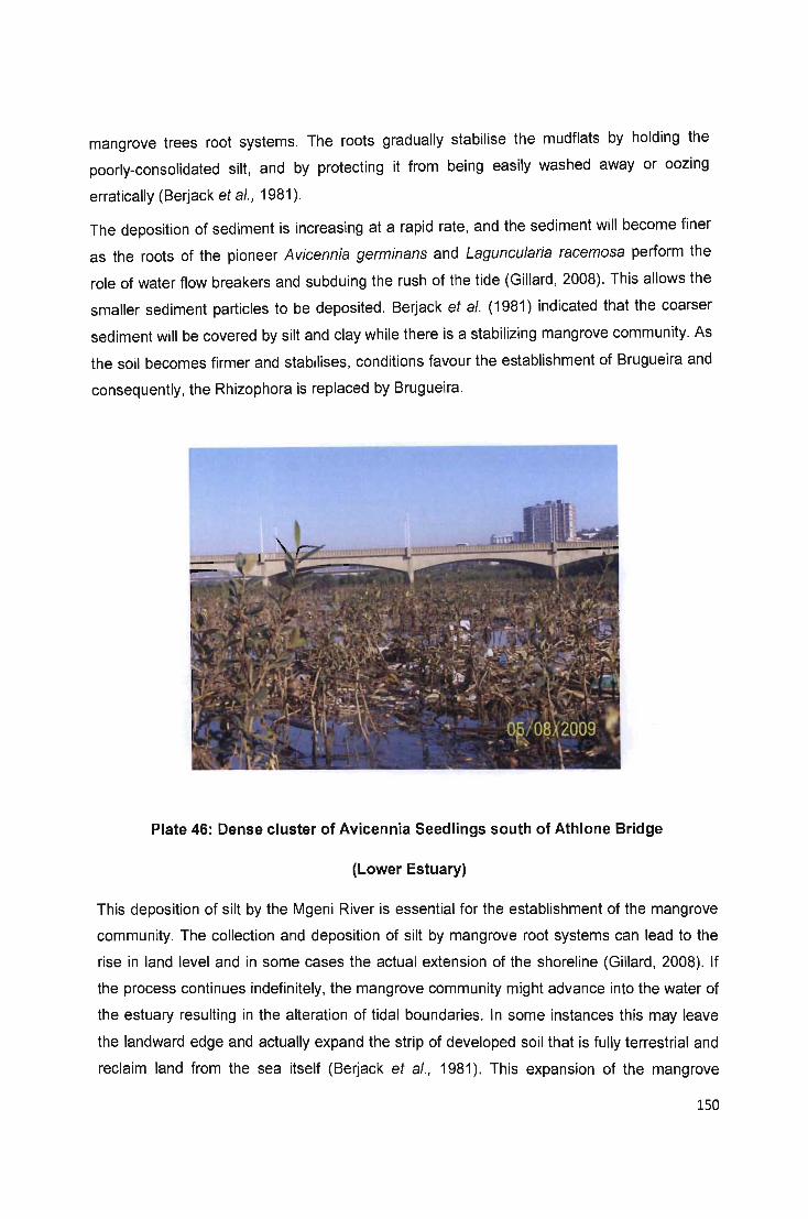
mangrove trees root systems. The roots gradually stabilise the mudflats by holding the
poorly-consolidated silt, and by protecting it from being easily washed away or oozing
erratically (Berjack et a/., 1981).
The deposition of sediment is increasing at a rapid rate, and the sediment will become finer
as the roots of the pioneer A vicennia germinans and Laguncularia racemosa perform the
role of water flow breakers and subduing the rush of the tide (Gillard, 2008). This allows the
smaller sediment particles to be deposited. Berjack et a/. (1981) indicated that the coarser
sediment will be covered by silt and clay while there is a stabilizing mangrove community. As
the soil becomes firmer and stabilises, conditions favour the establishment of Brugueira and
consequently, the Rhizophora is replaced by Brugueira.
Plate 46: Dense cluster of Avicennia Seedlings south of Athlone Bridge
(Lower Estuary)
This deposition of silt by the Mgeni River is essential for the establishment of the mangrove
community. The collection and deposition of silt by mangrove root systems can lead to the
rise in land level and in some cases the actual extension of the shoreline (Gillard, 2008). If
the process continues indefinitely, the mangrove community might advance into the water of
the estuary resulting in the alteration of tidal boundaries. In some instances this may leave
the landward edge and actually expand the strip of developed soil that is fully terrestrial and
reclaim land from the sea itself (Berjack et a/., 1981). This expansion of the mangrove
150
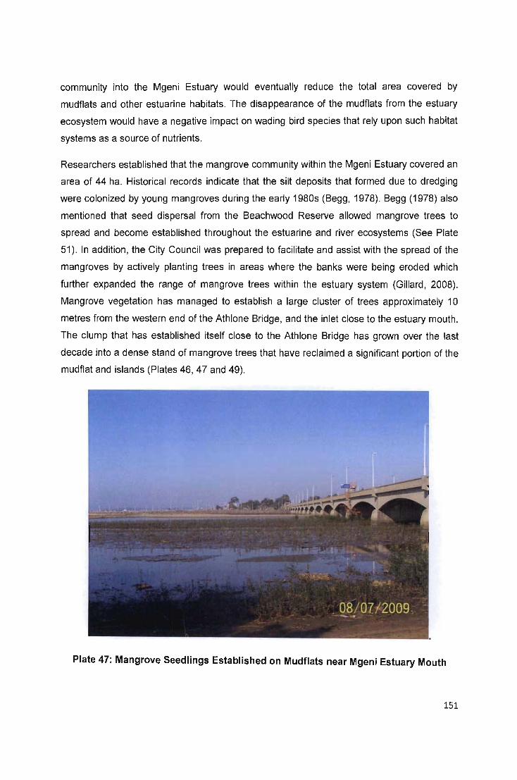
community into the Mgeni Estuary would eventually reduce the total area covered by
mudflats and other estuarine habitats. The disappearance of the mudflats from the estuary
ecosystem would have a negative impact on wading bird species that rely upon such habitat
systems as a source of nutrients.
Researchers established that the mangrove community within the Mgeni Estuary covered an
area of 44 ha. Historical records indicate that the silt deposits that formed due to dredging
were colonized by young mangroves during the early 1980s (Begg, 1978). Begg (1978) also
mentioned that seed dispersal from the Beachwood Reserve allowed mangrove trees to
spread and become established throughout the estuarine and river ecosystems (See Plate
51). In addition, the City Council was prepared to facilitate and assist with the spread of the
mangroves by actively planting trees in areas where the banks were being eroded which
further expanded the range of mangrove trees within the estuary system (Gillard, 2008).
Mangrove vegetation has managed to establish a large cluster of trees approximately 10
metres from the western end of the Athlone Bridge, and the inlet close to the estuary mouth.
The clump that has established itself close to the Athlone Bridge has grown over the last
decade into a dense stand of mangrove trees that have reclaimed a significant portion of the
mudflat and islands (Plates 46, 47 and 49).
Plate 47: Mangrove Seedlings Established on Mudflats near Mgeni Estuary Mouth
151

Umgeni Pari!
Mgeni River Estuary
Stamford
o 100 200 IIlOm
Prospect Hall l,vmAS OCEAN
Mgeni Estuary and Beachwood Mangrove
Swamps 1991 - 2008 Net
Land Cover Change
Plate 48: Mgeni Estuary and Beachwood Mangrove Swamps Land Cover Changes (1991-2008)
152
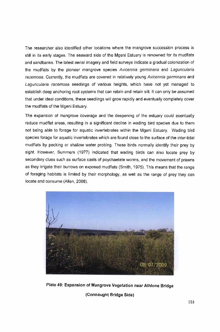
The researcher also identified other locations where the mangrove succession process is
still in its early stages. The seaward side of the Mgeni Estuary is renowned for its mudflats
and sandbanks. The latest aerial imagery and field surveys indicate a gradual colonization of
the mudflats by the pioneer mangrove species Avicennia germinans and Laguncu/aria
racemosa. Currently, the mudflats are covered in relatively young Avicennia germinans and
Laguncu/aria racemosa seedlings of various heights, which have not yet managed to
establish deep anchoring root systems that can retain and retain silt. It can only be assumed
that under ideal conditions, these seedlings will grow rapidly and eventually completely cover
the mudflats of the Mgeni Estuary.
The expansion of mangrove coverage and the deepening of the estuary could eventually
reduce mudflat areas, resulting in a significant decline in wading bird species due to them
not being able to forage for aquatic invertebrates within the Mgeni Estuary. Wading bird
species forage for aquatic invertebrates which are found close to the surface of the inter-tidal
mudflats by pecking or shallow water probing. These birds normally identify their prey by
sight. However, Summers (1977) indicated that wading birds can also locate prey by
secondary clues such as surface casts of poychaetete worms, and the movement of prawns
as they irrigate their burrows on exposed mudflats (Smith, 1975). This means that the range
of foraging habitats is limited by their morphology, as well as the range of prey they can
locate and consume (Allen, 2008).
Plate 49: Expansion of Mangrove Vegetation near Athlone Bridge
(Conn aught Bridge Side)
153
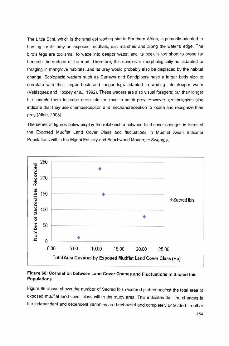
The Little Stint, which is the smallest wading bird in Southern Africa, is primarily adapted to
hunting for its prey on exposed mudflats, salt marshes and along the water's edge. The
bird's legs are too small to wade into deeper water, and its beak is too short to probe far
beneath the surface of the mUd. Therefore, this species is morphologically not adapted to
foraging in mangrove habitats, and its prey would probably also be displaced by the habitat
change. Scolopacid waders such as Curlews and Sandpipers have a larger body size to
correlate with their larger beak and longer legs adapted to wading into deeper water
(Velasquez and Hockey et a/., 1992). These waders are also visual foragers; but their longer
bills enable them to probe deep into the mud to catch prey. However, ornithologists also
indicate that they use chemoseception and mechanoreception to locate and recognize their
prey (Allen, 2008).
The series of figures below display the relationship between land cover changes in terms of
the Exposed Mudflat Land Cover Class and fluctuations in Mudflat Avian Indicator
Populations within the Mgeni Estuary and Beachwood Mangrove Swamps.
'tI 250
Q) • 'tI .. 0 200 (,) Q)
0:: .!{l
150 ."'"-.c '"
'tI • Sacred Ibis Q) .. (,)
100 (0 (J)
'0 • .. 50 Q)
.c E :::I • Z 0
0.00 5.00 10.00 15.00 20.00 25.00
Total Area Covered by Exposed Mudflat Land Cover Class (Ha)
Figure 66: Correlation between Land Cover Change and Fluctuations in Sacred Ibis Populations
Figure 66 above shows the number of Sacred Ibis recorded plotted against the total area of
exposed mudflat land cover class within the study area. This indicates that the changes in
the independent and dependent variables are haphazard and completely unrelated. In other
154
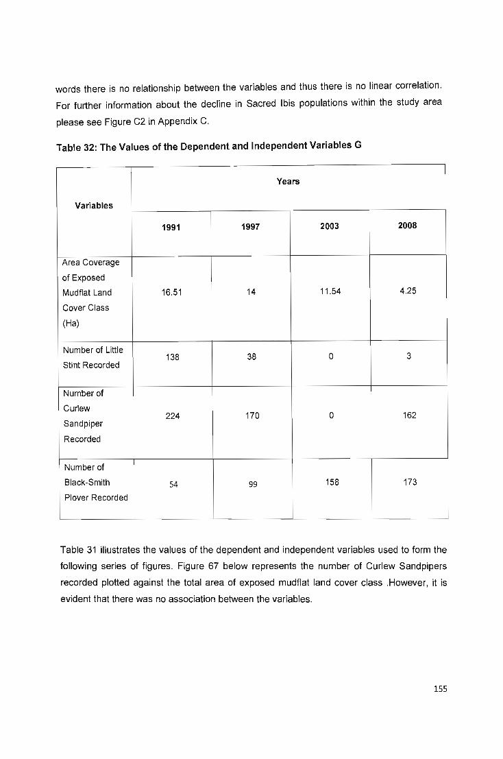
words there is no relationship between the variables and thus there is no linear correlation.
For further information about the decline in Sacred Ibis populations within the study area
please see Figure C2 in Appendix C.
Table 32: The Values of the Dependent and Independent Variables G
Years
Variables
1991 1997 2003 2008
Area Coverage
of Exposed
Mudflat Land 16.51 14 11 .54 4.25
Cover Class
(Ha)
Number of Little 138 38 0 3
Stint Recorded
Number of
Curlew 224 170 0 162
Sandpiper
Recorded
Number of
Black-Smith 54 99 158 173 Plover Recorded
Table 31 illustrates the values of the dependent and independent variables used to form the
following series of figures. Figure 67 below represents the number of Curlew Sandpipers
recorded plotted against the total area of exposed mudflat land cover class . However, it is
evident that there was no association between the variables.
155

(h 250
... Q) • .9-
200 ~ -c s:: l'a • (/)-c ~Q) 150 Q)'E .:0
• • Curlew Sandpipers
::J(") 100 uQ)
... 0:: 0 ... Q) 50 .Q
E ::J Z 0
0 5 10 15 20
Total Area Covered by Exposed Mudflat Land Cover Class (Ha)
Figure 67: Correlation between Land Cover Change and Fluctuations in Curlew
Sandpiper Population
Plate 50: Mangrove Vegatation Expansion- Former Mudflat Area
156
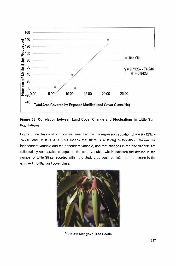
160
" 140 (I)
"E 120 o (J
~ 100
C 80 ~ .! 60
5 40 .... o a.. 20 (I)
.Q 0
~----------------------~~-------------• Little Stint
y= 9.7123x-74.246 R2= 0.8423
§ , ~ 00 Z _2lJ" ··}LU-----' ........... --...l.U...'-.LU-- -Uo<..........-- -"""' .......... '--~ ........
-40 Total Area Covered by Exposed Mudflat Land Cover Class (Ha)
Figure 68: Correlation between Land Cover Change and Fluctuations in Little Stint
Populations
Figure 68 displays a strong positive linear trend with a regression equation of 9 = 9.7123x-
74.246 and R2 = 0.8423. This means that there is a strong relationship between the
independent variable and the dependent variable, and that changes in the one variable are
reflected by comparable changes in the other variable, which indicates the decline in the
number of Little Stints recorded within the study area could be linked to the decline in the
exposed mudflat land cover class.
Plate 51: Mangove Tree Seeds
157

200 III 180 ... Qj
> 160 0 0:: .s: 140 .~ E'n 120 III Qj .'n '"" ... u 0 100 III U
- Qj a:la:: ... 80 0
60 ... Qj .ll 40 E ::J Z 20
0
0.00
~ ~
T
~ ...
5.00 10.00
~ ~ ~ -.
15.00 20.00
. SS Plover
y= -7.8746x+ 217.48 R2 = 0.7643
25.00
Total Area Covered by Exposed Mudflat land Cover Class (Hal
Figure 69: Correlation between Land Cover Change and Fluctuations in Black-Smith
Plover Population
Figure 69 displays the number of Black-Smith Plovers recorded plotted against the total area
covered by exposed mudflat land cover class. There is a strong negative linear trend
displayed in the figure with a regression equation of y = -7.8746x + 217.48 and R2 = 0.7643.
This indicates that changes in the one variable (Exposed Mudflats) are reflected in changes
in the other variable (Avian Indicators) in the opposite direction. This indicates that the Black
Smith Plover population has increased despite the decline in the area coverage of the
exposed mudflat land cover class.
Examination of the avian census data indicates that the number of Sanderlings is increasing
within the Mgeni Estuary and Beachwood Mangrove Swamps despite the decline in the area
covered by exposed mudflat habitats. This land cover class has been identified as the most
important foraging and roosting habitat for these couple of wading bird species. However,
the decline in exposed mudflat habitats appears not to be having a negative impact on the
Sanderling population (Plate 47). No figure was produced because Sanderlings are summer
migrants that visit the study area for a short period during the year, and large numbers of
these small wading birds only started to make regularly visits to the study area during the
late 1990s. Prior to this, there are inconsistent sightings of Sanderlings in small numbers
within the study area which were discounted.
158

In conclusion , the decline in the area coverage of the exposed mudflat land covers class is
undeniably linked to the expansion of mangrove vegetation into areas previously designated
as mudflat habitats. The decline in the area coverage of the exposed mudflats has also been
identified as the main cause behind the gradual decline in mudflat avian indicator
populations of Little Stints that rely on these exposed mudflat habitats for foraging and
roosting locations. This makes Little Stints ideal avian indicator species for this particular
land cover class. Further research discovered that the populations of other mudflat avian
indicator species were unaffected by the decline exposed mudflats and as a result they
cannot be considered as mudflat avian indicators in future studies. For example, Black-Smith
Plover numbers continued to increase despite the decline in the exposed mudflat land cover
class. This indicates that Black-Smith Plovers are not as reliant on mudflat habitats for
foraging and roosting as other mudflat avian indicator species because they have adapted to
a wider range of land cover classes.
5.23. Water Land Cover Classes within the Mgeni Estuary and Beachwood Mangrove Swamps
The researcher selected Pink-Backed Pelicans, White-Breasted Cormorants, and African
Darters as preferred indicators species for open water areas; and Goliath Herons and Little
Egrets as effective indicator species for shallow water areas. According to CWAC Bird
Census Data, Goliath Herons and Little Egret populations have increased between 1993 and
2008. This is seen in Figure B2 in the Appendix B.
Goliath Herons and Little Egrets have similar foraging techniques, whereby the bird wades
steadily through the shallows moving their feet in the mud and vegetation on the estuary
floor to tease out fish, amphibians and other prey species. White Egrets tend to forage in
shallow water of an average depth of 1 OOmm for their prey (See Appendix F). The reed beds
and aquatic vegetation along the edge of the water provide shelter for small fish seeking
refuge from aerial and surface predators. Fish make up a large portion of the Little Egrets
diet. The larger Goliath Heron can be found foraging in water of a depth of 325mm hunting
for larger fish species and amphibians (Velasquez and Hockey, 1992). Therefore, the
reduction in medium and deep water levels within the study area has led to an increase in
shallow water zones. This should stimulate an increase in Goliath Herons and Little Egrets
populations because conditions are more ideal for their foraging techniques. Neither species
swims or dives to catch their preferred prey (Plate 52).
159
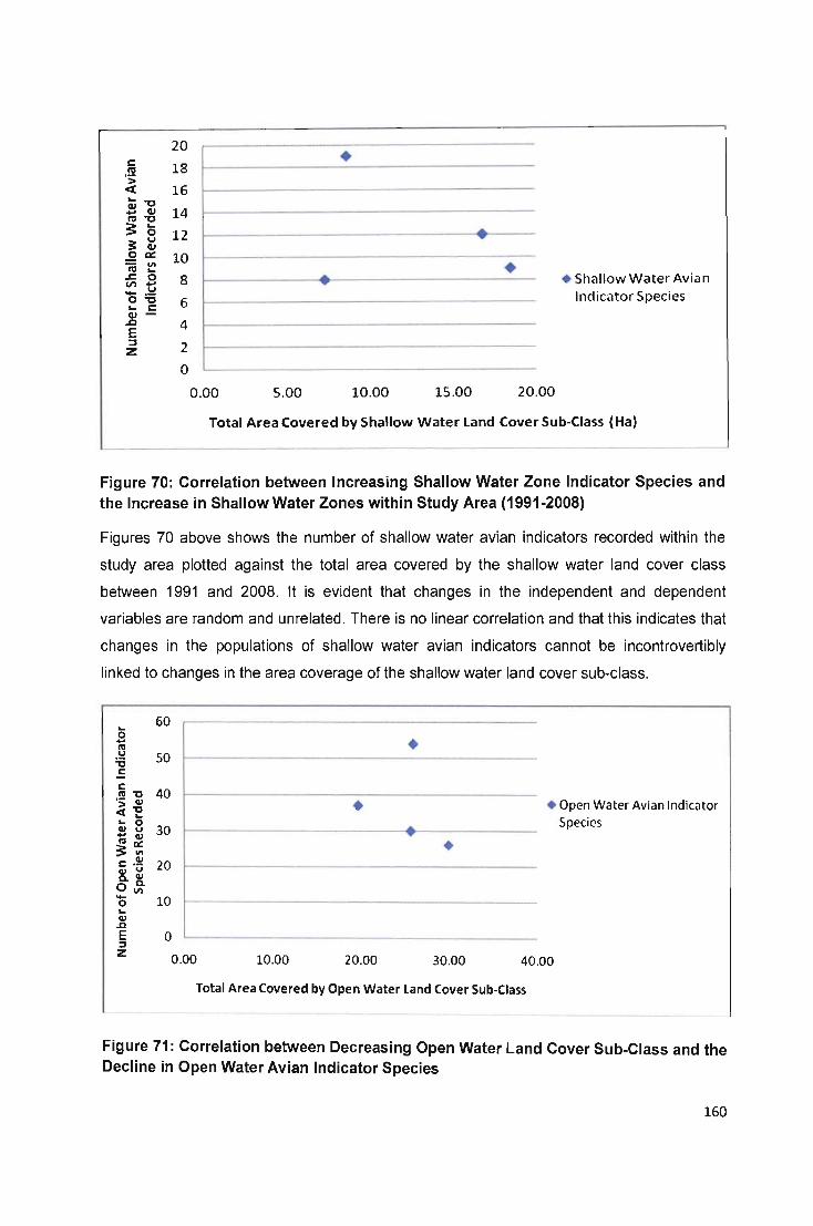
20
18
16 ""0 ~ cu 14 "'''0 ~ 6 ~ ~ 12
~ ~ 10 .r::. 0 8 ~ .1;; 0"0 .. C cu-.a E ::J Z
6
4
2
o 0.00
•
....
5.00 10.00 15.00
.....
•
20.00
• Shallow Water Avian Indicator Species
Total Area Covered by Shallow Water land Cover Sub·Class (Ha)
Figure 70: Correlation between Increasing Shallow Water Zone Indicator Species and the Increase in Shallow Water Zones within Study Area (1991-2008)
Figures 70 above shows the number of shallow water avian indicators recorded within the
study area plotted against the total area covered by the shallow water land cover class
between 1991 and 2008. It is evident that changes in the independent and dependent
variables are random and unrelated. There is no linear correlation and that this indicates that
changes in the populations of shallow water avian indicators cannot be incontrovertibly
linked to changes in the area coverage of the shallow water land cover sub-class.
60
50
; '0 40 'S; ~ ct ... ... 0
~ ~ 30 3: III
c'~ 20 8.li: o~ '0 10 ... GI
.J:l E :::I Z
o 0.00
•
•
10.00 20.00
•
30.00
• Open Water Avian Indicator Species
40.00
Total Area Covered by Open Water land Cover Sub·Class
Figure 71: Correlation between Decreasing Open Water Land Cover Sub-Class and the Decline in Open Water Avian Indicator Species
160
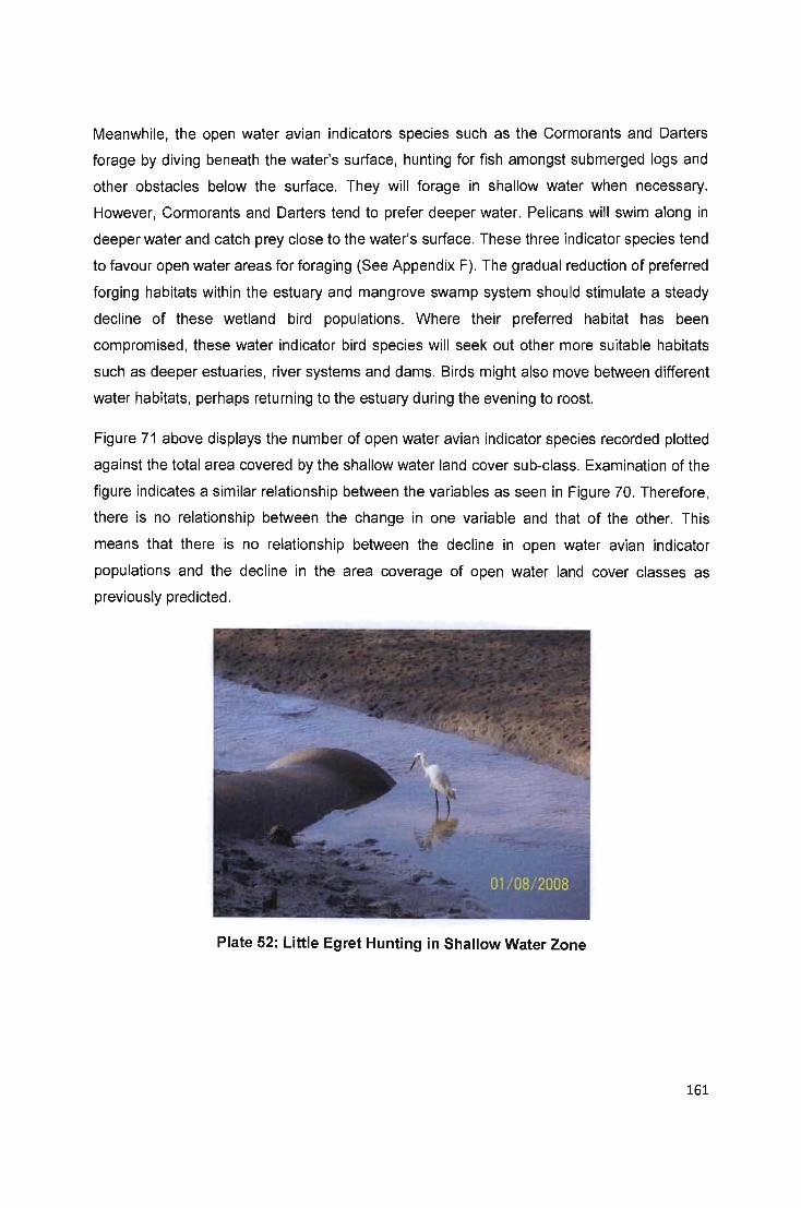
Meanwhile, the open water avian indicators species such as the Cormorants and Darters
forage by diving beneath the water's surface, hunting for fish amongst submerged logs and
other obstacles below the surface. They will forage in shallow water when necessary.
However, Cormorants and Darters tend to prefer deeper water. Pelicans will swim along in
deeper water and catch prey close to the water's surface. These three indicator species tend
to favour open water areas for foraging (See Appendix F). The gradual reduction of preferred
forging habitats within the estuary and mangrove swamp system should stimulate a steady
decline of these wetland bird populations. Where their preferred habitat has been
compromised, these water indicator bird species will seek out other more suitable habitats
such as deeper estuaries, river systems and dams. Birds might also move between different
water habitats, perhaps returning to the estuary during the evening to roost.
Figure 71 above displays the number of open water avian indicator species recorded plotted
against the total area covered by the shallow water land cover sub-class. Examination of the
figure indicates a similar relationship between the variables as seen in Figure 70. Therefore,
there is no relationship between the change in one variable and that of the other. This
means that there is no relationship between the decline in open water avian indicator
populations and the decline in the area coverage of open water land cover classes as
previously predicted .
Plate 52: Little Egret Hunting in Shallow Water Zone
161

" 7
GI
" 6 "" 0 ..... "" u
GI IX 5 c 0 "" GI 4 ::c
--<110. .....
.J:. ...
.!!! 3 .... .... + Go Heron
'0 C) .... 2 0
"" GI .Q 1 E
.... .... j
z 0
0.00 5.00 10.00 15.00 20.00
Total Area Covered by Shallow Water Land Cover Sub-Class (Ha)
Figure 72: Correlation between Land Cover Change and Fluctuations in Goliath Heron
Population
18 'tJ ~ 16
"tJ ..... ..
0 14 u ~ ex:
12 ... ~ .. QI) 10 LLI
~
• + LEgret 'E 8 :::i - 6 0 .. ~ 4 ..Q
... ~
E :l 2 z •
a 0 .00 5.00 10.00 15.00 20.00
Total Area Covered by Shallow Water land Cover Sub-Class (Ha)
Figure 73: Correlation between Land Cover Change and Fluctuations in Little Egret
Population
162
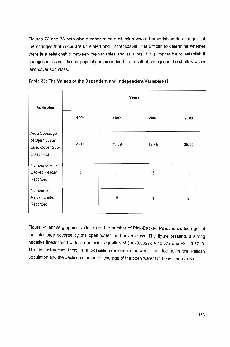
Figures 72 and 73 both also demonstrates a situation where the variables do change, but
the changes that occur are unrelated and unpredictable. It is difficult to determine whether
there is a relationship between the variables and as a result it is impossible to establish if
changes in avian indicator populations are indeed the result of changes in the shallow water
land cover sub-class.
Table 33: The Values of the Dependent and Independent Variables H
Years
Variables
1991 1997 2003 2008
Area Coverage
of Open Water 26.00
Land Cover Sub-25.69 19.75 25.99
Class (Ha)
Number of Pink-
Backed Pelican 0 1 3 1
Recorded
Number of
African Darter 4 5 1 2
Recorded
Figure 74 above graphically illustrates the number of Pink-Backed Pelicans plotted against
the total area covered by the open water land cover class. The figure presents a strong
negative linear trend with a regression equation of y = -0.3827x + 10.573 and R2 = 0.8749.
This indicates that there is a possible relationship between the decline in the Pelican
population and the decline in the area coverage of the open water land cover sub-class.
163

3.5 \/I C 1'0 3 .~ Qj 0.. 2.5 "0 Qj .¥"O U Qj 2 1'0'0 co "" I 0 .¥ U
1.5 .5 Qj 0..0::
'0 1 "" Qj .,g
E O.S ::J Z
0
o
... \ \ \ \~ '\
"" "" 10 20 30
• PB Pelcian
y = -0.3827x + 10.573 R2 = 0.8749
Total Area Covered by Open Water land Cover Sub-Class
Figure 74: Correlation between Land Cover Change and Fluctuations in Pink-Backed
Pelican Population
Figure 75 below shows the number of White-Breasted Cormorant recorded plotted against
the area covered by the open water land cover sub-class. It is evident that the changes in
the independent and dependent variable appear to be arbitrary and completely unrelated to
each other. Therefore, there is no relationship between the decline in the area coverage of
open water areas and the gradual disappearance of White-Breasted Cormorants.
Figure 76 below is displays a moderately strong positive linear trend with a regression
equation of 9 = 0.4191x - 7.2093 and R2 = 0.4984. A correlation coefficient of +0.4984
indicates that a decrease in the independent variable should result in a comparable
decrease in the dependent variable. Therefore, the decline in the area coverage of the open
water land cover sub-class might be responsible for the decline in the population of African
Darter.
164
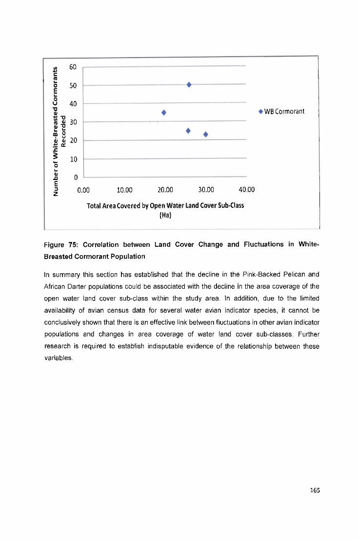
III ... C tel .. 0 E .. 0 u
" Q/
... " III Q/
tel" Q/ .. .. 0 ~ u Q/ Q/
.~ a: s:. ~ .... 0 .. Q/
.Q
E j
Z
60
50
40
• 30
• • 20
10
0
0.00 10.00 20.00 30.00 40.00
Total Area Covered by Open Water land Cover Sub·Class (Ha)
• WB Cormorant
Figure 75: Correlation between Land Cover Change and Fluctuations in White
Breasted Cormorant Population
In summary this section has established that the decline in the Pink-Sacked Pelican and
African Darter populations could be associated with the decline in the area coverage of the
open water land cover sub-class within the study area. In addition, due to the limited
availability of avian census data for several water avian indicator species, it cannot be
conclusively shown that there is an effective link between fluctuations in other avian indicator
populations and changes in area coverage of water land cover sub-classes. Further
research is required to establish indisputable evidence of the relationship between these
variables.
165

Plate 53: Shallow Water in the Mgeni Estuary
'0 6
Q)
'0 ... 5 0
(,) Q)
0:: ... 4 Q) T -... ('CI
c 3 c:
('CI (,)
;e 2 c( ... 0 ...
1 Q) .Q
/ • African Darter
/ y= 0.4191x - 7.2093 I-------------/-r--~T..--- R2 = 0.4984
E :J
0 Z
0 5 10 15 20 25 30
Total Area Covered by Open Water Land Cover Sub..class (Ha)
Figure 76: Correlation between Land Cover Change and Fluctuations in African Darter
Population
166

Chapter Six
Conclusion and Recommendations
6.1. Inconsistencies in the Avian Census Data Set Acknowledged
Whereas the land cover data was gathered and processed by the researcher off aerial
survey imagery using GIS software tools; the avian census data was the result of Waterbird
Counts (CWAC) project field surveys undertaken by the University of Cape Town's Avian
Demographic Unit, and over which the researcher had absolutely no control (Wheeler,
2008). This study therefore had no other option but to utilise the only credible avian census
data - the Waterbird Counts (CWAC) project - with all its potential limitations.
A review of the study findings has demonstrated that the limited counts on certain bird
species in some instances undermined the statistical validation process. The basic rule of all
research is to obtain the largest set of data samples possible to ensure that the statistical
accuracy of the information is enhanced. Conversely, a limited set of sample data could
compromise the scientific accuracy or relevancy of the eventual findings of any given study.
In this instance certain wetland avian indicator counts were either too sparse, or in other
instances leaned towards a potential for human error. The Coordinated Waterbird Counts
(CWAC) project undertook regular mid-summer and mid-winter censuses of wetland sites all
around South Africa, including the Mgeni Study Area. Wheeler (2008) indicates that the
regular six-monthly counts are conducted by groups of experienced ornithologists and
'volunteers' . This study has shown that more frequent avian counts, with less potential
human inaccuracies would clearly enhance the validity of future study conclusions.
There are two main criteria used for evaluating the quality of avian data sets used during a
particular study. Each of these criteria actually relates most strongly to the quality of the
process by which data is collected, and the methods used during the process of collecting
the data (Rumsey, 2003). However, the available avian data sets used for the study area are
limited to the findings of two potentially biased bi annual surveys. As such it is impractical to
167

precisely determine changes in avian populations based on partially compromised avian
data sets.
Firstly, the researcher suspected that the avian census was biased, being data that is
occasionally over measured or under measures the true result (Rumsey, 2003). Bias can
occur anywhere during the design or implementation of a particular study. Bias can be
caused by a bad measurement techniques or human error (Rumsey, 2003). Basic human
error has been identified as the most obvious cause of irregularities and inconsistencies in
the avian census data used. Counters are responsible for the identification and recording of
the number of birds sighted during field surveys. The Counters have a varying degree of
avian knowledge, practically amongst part-time bird enthusiasts and volunteers, which can
lead to mistakes during identification and the recording of sightings. Mistakes do occur on a
regular basis according to ornithologists (Allen, 2008; Gillard, 2008). This can lead to a false
representation of the numbers of wetland birds within the study area, especially when one is
using only two counts annually.
The CWAC guidelines state that numbers of birds should be estimated when the numbers
are relatively large (+/- 1000), the birds are moving rapidly or flying, there is a chance of a
disturbance or birds are crowded and not all the birds are clearly visible. Ornithologists and
experienced Counters promote the use of a method for estimating numbers of birds in large
flocks, either in flight or on the ground, known as the "Block Method". Basically, this method
involves the super imposing of a fictional or actual block of a certain size onto or within a
large flock of birds (Wheeler, 2008). Each block should have 10, 20, 100 or some other
round number of individual birds assigned to it. However, inexperienced Counters tend to
underestimate the number of birds present within a block when they are estimating the size
of a large flock of birds (+/- 100 individuals). Wheeler (2008) states that experience is vitally
important during the application of this counting method in the field, and regular practise is
require perfecting this method.
Given the background as set out above, the researcher assessed the available data sets
and disregarded potentially flawed data in favour of data which appeared to have a
reasonable and acceptable consistency. The researcher did not totally disregard the flawed
data sets, but allowed himself to be influenced by the general trend identified, accepting that
the results were not necessarily statistically validated. Had more frequent surveys been
undertaken, the validity of the study results would have certainly been enhanced.
168

The more reliable data sets utilised in reaching a conclusion generally supported the thesis
that changes in land cover can be linked to a corresponding fluctuation in wetland avian
species, the basic premise of this study. Therefore it can be stated that specific wetland
avian bird species have the potential to be utilised as an effective monitoring tool with which
to help assess and predict land cover changes within estuarine and mangrove swamps
within Southern Africa.
6.2. General Conclusion
Estuaries and mangrove swamps are recognised as valuable ecosystems because of the
variety of ecological and economic functions they perform. These ecosystems benefit the
natural environment and mankind and deserve appropriate management and conservation.
Scientists, biologists, physicists and other academics all recognize the need for an effective
method of monitoring the health and integrity of estuarine and mangrove swamp ecosystems
to ensure that these ecosystems are conserved and managed appropriately for the benefit of
future generations.
This study sought to establish whether wetland indicator bird species could be used as an
effective monitoring system to help assess and predict land cover changes within estuaries
and mangrove swamps within Southern Africa. The Mgeni Estuary and adjacent Beachwood
Mangrove Swamps were chosen as an appropriate study area. The researcher recognized
there were several potential problems that might arise due to the effects of tidal fluctuation
within the Mgeni Estuary and Beachwood Mangrove Swamp study area, and issues of
reliability arising from irregularities in the avian census database. These problems could
have undermined the legitimacy of the study if appropriate measures had not been
introduced to ensure they were addressed effectively. This process provided the researcher
with a solid platform upon which to develop a substantial argument in favour of the
relationship between estuarine and mangrove swamp land cover change, and the effects of
such land cover change on wetland avian indicator populations.
Fluctuations in the populations of wetland avian indicator species were investigated by this
study. It was discovered that that bird populations fluctuated significantly over time within the
Mgeni Estuary and Beachwood Mangrove Swamp study area. Further research determined
that the prevalence of specific indicator species was associated with seasonality rather than
land cover change. However, other species showed signs of population decline that could be
linked to changes in a particular land cover classes. These assumptions were verified
through statistical analysis known as correlation coefficiency. This is the measure of how
169
closely two variables change in relationship to each other. In this case, the number of birds
recorded plotted against the time index. Finally, the researcher concluded that merely
assessing and interpreting fluctuations in bird populations identified in avian census data
was not sufficient enough to provide accurate and reliable data on wetland bird populations.
An effort should be made to supplement these data sets with long term data on reproductive
success and demographic traits according to local ornithologists (Allen, 2008).
Changes in land cover classes and sub-classes were investigated during this study. The
Mgeni Estuary and adjacent Beachwood Mangrove Swamps are dynamic ecosystems that
are affected by natural phenomena, and human activities throughout the entire river
catchment area. This study focused primarily on the immediate vicinity of the estuary and the
mangrove swamps. However, outside influences could not be totally ignored when
examining the causes of land cover change. The study attempted to identify significant land
cover change within the study area over the past eighteen years through the assessment of
a series of aerial survey imagery. GIS analysis of aerial imagery allowed the researcher to
successfully categorize and map different land cover types within the study area, and was
used to calculate the total area covered by each land cover class and sub-class, in relation
to the fixed total coverage of the study area. This provided the opportunity for the
examination and recording of changes in terms of land cover within the study area, within a
specific study period , all relative to a fixed area base. Once again , the researcher clarified
the findings by attempting to discover the correlation between the total area covered by the
land cover classes, and sub-classes, plotted against the time index. In conclusion , the study
established that changes in specific adjacent land cover classes and sub-classes; were the
result of the opportunity created by changes in adjacent land cover classes. For example,
coastal forest and woodland which had an impact upon adjacent grassland and scrubland
areas, or the expansion of mangroves which resulted in the colonisation of mudflats. One
example of significant human intervention would be the restricted water flow and sediment
load due to a controlled outflow program introduced by Inanda Dam management.
This study provided sufficient evidence to suggest that both human and naturally induced
changes within the estuarine and mangrove ecosystems, as reflected by changes in some
land cover classes, had an impact on specific wetland bird populations. However, to confirm
this theory, the researcher correlated the number of avian indicators recorded against the
total area covered by the specific land cover class, or sub-class, considered by the
researcher and ornithologists to be their ideal foraging, roosting or breeding habitats. This
assisted in validating the theory that, for instance, the decline in the exposed mudflat land
cover class was linked to the expansion of the mangrove vegetation land cover class and
170

island mangrove vegetation land cover sub-classes, and was directly responsible for the
gradual decline in, for instance, the Little Stint population. On the otherhand, the increase in
the population of the Water Dikkop is reflected in the increased area of reed beds, marshes
and grassland land cover classes within the study period.
Secondly, a close examination of aerial imagery revealed the progressive expansion of the
mangrove community into the estuary and the lower reaches of Mgeni river ecosystem. The
researcher recorded that the pioneering mangrove species, Avicennia germinans (Black
Mangrove) and Laguncu/aria racemosa (White Mangrove), have managed to steadily
colonize large portions of the once prominent mudflats during several field surveys. This
significant change in land cover within the study area has impacted on mudflat avian
indicator populations. Mudflat indicator species, or wading bird species, cannot forage for
aquatic invertebrates in open water or densely vegetated habitats. Wading bird species are
adapted to foraging for aquatic invertebrates which are found close to the surface of the
intertidal mudflats. This steady land cover change will inevitably lead to a decline in mudflat
habitats, and a consequent reduction of the wading bird species which are especially
dependent upon such habitats.
Certain avian indicator species proved to be very effective in their designated role as
indicator species; others indicated potential given an acceptable level of avian census data;
whilst others appeared to be ineffective, perhaps due to a greater level of environmental
adaptability - see Appendix I.
However, after careful analysis of the eventual findings of this study, the researcher has
concluded that despite a robust and rigorous assessment of all assessable avian census
databases, and the examination and processing of relevant aerial imagery, further in-depth
research is required to establish an meaningful link between land cover change, and the
fluctuations of wetland bird populations with the estuarine ecosystem.
In conclusion, this study has merely touched the surface of an interesting field of research,
the results of which suggested a need to delve deeper in order to establish indisputable
evidence confirming that a direct link exists between land cover change, resulting in
fluctuations in wetland avian populations. However, before further research is undertaken
into the utilization of bird species as environmental monitoring tools, a more concise and
extensive avian census database must be developed to provide researchers with an
appropriate avian census data set. Recent work undertaken by the Avian Demographic Unit
at the University of Cape Town is a significant step in the right direction.
171
6.3. Future Applications of this Study
This study has provided a spatial and descriptive historical land cover database of the Mgeni
Estuary and Beachwood Mangrove Swamps over the past eighteen years. This baseline
information can assist in the development of an improved environmental management
regime for other estuarine and mangrove ecosystems throughout Southern Africa. The study
has successfully shown that wetland avian species can be used to monitor environmental
changes within the Mgeni Estuary and adjacent Beachwood Mangrove Swamps.
By highlighting the value for regular monitoring of wetland avian species populations within
estuarine and mangrove ecosystems, this research has contributed to the body of local
knowledge surrounding methods of conservation management and the protection of an
environmentally sensitive ecosystem type. It was this desire to help make a contribution to
the conservation of natural ecosystems which inspired the researcher to embark upon this
study within the Mgeni Estuarine and Beachwood Mangrove Swamp ecosystem.
The land cover database, and the use of wetland bird species as a system of monitoring
land cover change within an ecosystem, as developed during this study, can also be used in
the following applications:
The concepts developed by this study can be applied as an environmental tool. The
results of this study can be applied during environmental management such as the
analysis of further changes of habitats within the study area. The data base that has
been developed during this course of this study can be used by the eThekwini
Municipal Environmental division who require reliable information on land cover
changes taking place within protected DMOSS areas within the City.
The historical land cover data base that was developed during this study can be
utilised by both the public and private sectors in environmental planning work within
the Mgeni Estuary and Beachwood Mangrove Swamp study area and the
surrounding area.
The land cover data base developed during this study can be combined with other
studies undertaken in the Albert Falls area by Yemane (2003), Midmar Dam sub
catchment by Rivers-Moore (1997) and the Karkloof SUb-catchment area by Weyer
(2000) to model land cover change within the entire Mgeni catchment area
172

This study further reaffirmed the usefulness of avian indicator species within natural
ecosystems. The United States Environmental Protection Agency has been utilising
various bird species as a monitoring tool within a wide variety of different habitats for
decades.
In addition, the study contributed to the greater body of knowledge about tools and
methods that enviromentalists can use to monitor the health and integrity of our
natural world.
This dissertation on land cover change within the Mgeni Estuary and Beachwood
Mangrove Swamps, and the use of wetland avian indicator species to monitor such
changes, will be made available to other researchers and decision makers interested in
environmental management planning and policy making within the Mgeni Estuary and
Beachwood Mangrove Swamps.
6.4. Recommendations
As a result of this study the following are recommended:
That environmental departments, boards and organisations implement a systematic
policy of monitoring wetland bird populations as indicators of environmental change
within wetland and estuarine ecosystems as part environmental management plan
for both local and national levels.
That organisations and groups that are responsible for the collection of the CWAC
Wetland Bird Survey data should be encouraged by these departments, boards and
other organisations to undertake more regular surveys throughout the year. If
surveys were conducted in such a manner, this would provide a better overall
understanding of the fluctuations in wetland bird populations throughout Southern
Africa and provide a more reliable source of avian data.
That the more sensitive ecosystems should be subjected to more regular structured
aerial surveys to help provide essential raw data for monitoring purposes.
That Environmental Planners should consider using avian indicators more regularly
to assist with the assessment of the health and integrity of natural ecosystems.
That, during similar land covers use and cover change analysis studies, the
researcher should gather and analyse all available remote sensing data. Satellite
173

imagery has several advantages over aerial imagery in the future. These include the
following:
1. Commercially available to general public
2. Greater aerial extent and accuracy than aerial photographs.
3. Satellite imagery comes in a digital format.
4. Satellite imagery allows regular repetitive coverage, while aerial surveys are
infrequent.
5. Regular and predicable distortion.
6. A greater wavelength range.
That locally manufactured remote controlled air vehicles (drones) equipped with
cameras and other sensors should be used to enable them to cheaply and easily
conduct aerial surveys on a regular basis. The capture of aerial imagery from aircraft
is expensive and undertaken on an irregular basis.
174

References
Anderson, J.R, Hardy, E.E., Roach, J.T. and Witmer, RE. 1976. A Land Use and Land Cover Classification System for Use with Remote Series Data. Geological Survey Professional Paper 964, A Revision of Land Use Classification System as Presented in US Geological Survey Circular 671, United States Government
Printing Office, Washington.
Allen, D. 2008. Interview with David Allen, Curator of Durban Museum of Natural History,
about Wetland Bird Species. 6/07/2008. Durban
Begg, G.W. 1978. The Estuaries of Natal. Natal Town and Regional Planning Report 41: 657
pp.
Berjak, P., Campbell, GK, Huckett, B. and Pam menter, N. 1981. In the Mangroves of Southern Africa. Wildlife Society of Southern Africa (Natal Branch), Durban: 1-
72 .
Birdlife International. 2008. Birds are Very Useful Indicators for Other Kinds of Biodiversity, http://www.birdlife.org/action/science/indicators/birds_asjndicators.html . Accessed 6/04/2009 at 8:56pm: p 1-12
Botes, R .2009. Interview with Riaan Botes, GIS Solutions about GIS application and Land Cover Change Assessments. 10/11/2009
Campbell , J.B. 1983. Mapping the Land: Aerial Imagery for Land Use Information. Resource Publications, Washington.
Canterbury, G.E. , Martin, T.E. , Petit, D.R , Petit, L.J. and Bradford , D.F. (2000) Bird Communities and Habitat as Ecological Indicators of Forest Conditions in Regional Monitoring. Conservation Biology, Vol. 14, No. 2, pp. 544-558Chittenden. H.2007. Roberts Bird Guide: A Comprehensive Field Guide to Over 950 Bird Species in Southern Africa. The Trustees of the John Voelcker Bird Book Fund: 1-456.
Carver, A.J. 1981. Air Photography for Land Use Planning. Department of Conservation and Extension, Salisbury, Zimbabwe.
Christian, RR. 2008. The Value of Healthy Estuaries. http://www.actionbioscience.org/environmentlchristian.html. Accessed 10/12/2009 at 11 :34 pm: 1-5
Cooper, J.A.G. 1999. The Role of Extreme Floods in Estuary-Coastal Behaviour: Contrasts between River- and Tide-Dominated Microtidal Estuaries. Coastal Studies Research Group, School of Environmental Studies, University of Ulster, Cromore Road, Coleraine, County Londonderry, Northern Ireland BT52 1 SA, UK
175
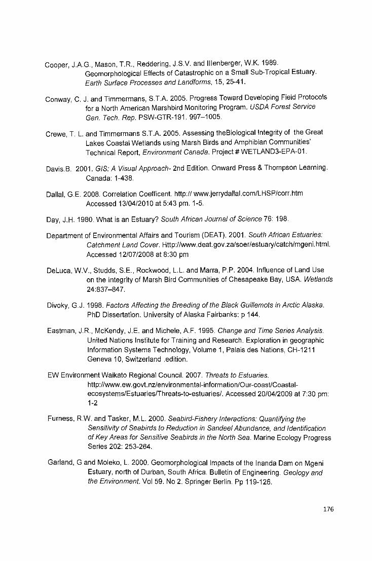
Cooper, JAG., Mason, T.R , Reddering, J.S.v. and Illenberger, W.K. 1989. Geomorphological Effects of Catastrophic on a Small Sub-Tropical Estuary.
Earth Surface Processes and Landforms, 15, 25-41.
Conway, C. J. and Timmermans, S.TA 2005. Progress Toward Developing Field Protocols for a North American Marshbird Monitoring Program. USDA Forest Service
Gen. Tech. Rep. PSW-GTR-191 . 997-1005.
Crewe, T. L. and Timmermans S.TA 2005. Assessing theBiologicallntegrity of the Great
lakes Coastal Wetlands using Marsh Birds and Amphibian Communities' Technical Report, Environment Canada. Project # WETlAND3-EPA-01 .
Davis.B. 2001. GIS: A Visual Approach- 2nd Edition. Onward Press & Thompson learning.
Canada: 1-438.
Dallal, G.E. 2008. Correlation Coefficent. http://www.jerrydallal.com/lHSP/corr.htm
Accessed 13/04/2010 at 5:43 pm. 1-5.
Day, J.H. 1980. What is an Estuary? South African Journal of Science 76: 198.
Department of Environmental Affairs and Tourism (DEAT). 2001 . South African Estuaries: Catchment Land Cover. Http://www.deat.gov.za/soer/estuary/catch/mgenLhtml.
Accessed 12/07/2008 at 8:30 pm
Deluca, W.V., Studds, S.E. , Rockwood, l .l. and Marra, P.P. 2004. Influence of land Use on the Integrity of Marsh Bird Communities of Chesapeake Bay, USA. Wetlands
24:837-847.
Divoky, G.J. 1998. Factors Affecting the Breeding of the Black Guillemots in Arctic Alaska. PhD Dissertation. University of Alaska Fairbanks: p 144.
Eastman, J.R, McKendy, J.E. and Michele, A.F. 1995. Change and Time Series Analysis.
United Nations Institute for Training and Research . Exploration in geographic I nformation Systems Technology, Volume 1, Palais des Nations, CH-1211 Geneva 10, Switzerland .edition.
EW Environment Waikato Regional Council. 2007. Threats to Estuaries. http://www.ew.govt.nzlenvironmental-information/Our-coasUCoastalecosystems/EstuarieslThreats-to-estuaries/. Accessed 20104/2009 at 7:30 pm: 1-2
Furness, RW. and Tasker, M.l. 2000. Seabird-Fishery Interactions: Quantifying the Sensitivity of Seabirds to Reduction in Sandeel Abundance, and Identification of Key Areas for Sensitive Seabirds in the North Sea. Marine Ecology Progress Series 202: 253-264.
Garland, G and Moleko, l . 2000. Geomorphological Impacts of the Inanda Dam on Mgeni
Estuary, north of Durban, South Africa. Bulletin of Engineering. Geology and the Environment. Vol 59. No 2. Springer Berlin. Pp 119-126.
176
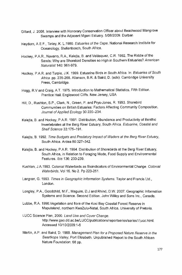
Gillard, J. 2008. Interview with Honorary Conservation Officer about Beachwood Mangrove Swamps and the Adjacent Mgeni Estuary. 5/08/2009. Durban
Heydorn, AE.F. , Tinley, K. L.1980. Estuaries of the Cape. National Research Institute for
Oceanology, Stellenbosch , South Africa.
Hockey, PAR, Navarro, RA , Kalejta, B. and Velasquez, C.R 1992. The Riddle of the Sands: Why are Shorebird Densities so High in Southern Estuaries? American
Naturalist 140: 961-979.
Hockey, P.AR. and Turpie, J.K. 1999. Estuarine Birds in South Africa. In: Estuaries of South Africa. pp. 235-268. Allanson , B.R. & Baird , D. (eds) . Cambridge University
Press, Cambridge.
Hogg, RV and Craig, AT. 1975. Introduction to Mathematical Statistics. Fifth Edition . Prentice Hall. Englewood Cliffs. New Jersey, USA
Hill , D., Rushton, S.P. , Clark, N., Green , P. and Prys-Jones, R. 1993. Shorebird Communities on British Estuaries: Factors Affecting Community Composition. Journal of Applied Ecology 30:220-234 .
Kalejta , B. and Hockey, PAR 1991. Distribution , Abundance and Productivity of Benthic Invertebrates at the Berg River Estuary, South Africa . Estuarine, Coastal and Shelf Science 33:175-191 .
Kalejta, B. 1992. Time Budgets and Predatory Impact of Waders at the Berg River Estuary, South Africa. Ardea 80:327-342.
Kalejta, B. and Hockey, PAR. 1994. Distribution of Shorebirds at the Berg River Estuary, South Africa, in Relation to Foraging Mode, Food Supply and Environmental Features. Ibis 136: 233-239.
Kushlan , JA1993. Colonial Waterbirds as Bioindicators of Environmental Change. Colonial Waterbirds, Vol 16. No 2. Pp 223-251.
Langran , G. 1993. Times in Geographic Information Systems. Taylor and Francis Ltd ., London.
Longley, P.A., Goodchild, M.F., Maguire, D.J and Rhind, D.W. 2007. Geographic Information Systems and Science. Second Edition. John Willey and Sons Inc., Canada.
Lubbe, RA 1996.vegetation and flora of the Kosi Bay Coastal Forest Reserve in Maputaland, northern KwaZulu-Natal , South Africa. University of Pretoria.
LUCC Science Plan, 2000. Land Use and Cover Change. http://www.geo.dd.ac.be/LUCC/publications/reportseries/series1/;ucc.html. Accessed 10/10/2009: 1-6
Martin, AP. and Baird, D. 1988. Management Plan for a Proposed Nature Reserve in the Swartkops Valley, Port Elizabeth. Unpublished Report to the South African Nature Foundation: 68 pp.
177

Marus, T., Ealles, K. and Wildschut, A.1996. Down to Earth: Land Demands in the New South Africa. Indicator Press, Durban.
Manoj ,N.T, Umikrishinan ,A.S, and D.Sundar. 2009. Tidal Asymmetry in the Mandai and Zaari Estuaries, the West Coast of India. Journal of Coastal Research. 25(6);
1107-1197
McCarthy.T. and Rubidge, B. 2006. The Story of Earth and Life: A Southern African Perspective on a 4.6 Billion Year Journey. School of Geosciences, University
of Witwatersrand. Struik Publishers. Cape Town: 1-333
McCally, P. 2007. Hydrological Effects of Dams: Silent Rivers: The Ecology and Politics of Large Dams. http://www.internationalrivers.org/en/node/1640 . Accessed
10105/2010 at 12:30 pm. 1-20
McNae, W.1963. Mangrove Swamps in South Africa. Journal of Ecology 51: 1-25
Meyer, W.B.1995. Past and Present Land Use and Land Cover in the USA. In : Eddy J.A., Consequences: The Nature and Implications of Environmental Change. Volume
1, No.1 Signaw Valley State University, USA. http://www.gerio.org/CONSEQUENCS/spring95/Land.html.
Meerkerk, D.N.1997. Land Cover Classification in Two Districts of the Northern Province. Land Management and Rural Development Program, Occasional Paper, number 5, University of the North, South Africa.
Mornat, P.O. and Quinn, N.W. 1999. Influence of Man and Management of South African Estuaries. In Estuaries of South Africa. Pp. 289-320. Allanson, B.R. & Baird, D. (eds). Cambridge University Press, Cambridge.
Morrison, M. L. 1986. Bird Populations as Indicators of Environmental Change. Curro Ornithology 3:429-451
Mitchel, R.J. 1981 . A Guide to Air Photo Interpretation: for Land Use Planners. Department of Conservation and Extension, Salisbury, Zimbabwe.
Miller, T.G. 2004. Living in the Environment: Principles, Connections, and Solutions. St Andrews Presbyterian College, Thomson Brooks/Cole :1- 756
National Parks Service. 2005. Measuring Vegetation Health. US Department of the Interior. http:// www.nps.gov/ .. .Icape-cod-ecosystem-monitoring-program-reports-andpublications.htm. Accessed 12/05112010 at 12:23 pm
Newman, K. 2006. Newman's Birds of Southern Africa. MacMillan South Africa. Johannesburg. South Africa
Peuquet, D.J. 1999. Time in GIS and Geographical Databases. In Longley, PA, Goodchild,M.F. , Maguire,D. , and Rhind, D.(eds). Geographic Information Systems: Principles and technical Issues, V.I ,pp.91-103, John Willey and Sons Inc., Canada.
178

Peakall, D.B. 2004. Avian data bases in their use in environmental assessment. Ecotoxicology. Vol 9. No 4. Springer Netherlands. Pp 239-253.
Rumsey, 0.2003. Statistics for Dummies. Dummies.Com. p: 1-384
Rivers-Moore, NA 1997. The Use of GIS to Examine Changes in Land Use Patterns in the Midmar Catchment, M.Sc. Thesis, School of Environmental and Development,
University of Natal, Pietermaritzburg.
Slack, J.C.1992. Colonial Waterbirds: Status and Trends of Selected Vertebrate Resources
in Galveston Estuary: Birds and Alligators, gbic.tamug.edu/gbeppubs/33/gbnep_33_61_75.pdf, Accessed 04/04/2009 at 7:23 pm: 1-5
Smith, M.M. 1981 . The Seahorse of the Knysna Lagoon. African Wildlife 35(6): 5-7.
Summers, R.W. 1977. The Distribution, Abundance and Energy Relationships of Waders, Aves: Charadris, at Langebaan Lagoon. Transactions of the Royal Society of South Africa 42: 483-495.
Schroem, J., de W~t, J. and Turpie, J.K .2005. Value of the Mngazana Estuary Mangroves.
http://www.fitzpatrick.uct.ac.za/docs/resource2.html. Accessed 12/06/2009 at 7:30pm: 1-2
South African River Health Programme. 2002. Lower uMgeni Resource Unit. State of Rivers Report: uMgeni River and Neighbouring Rivers and Streams.
Http://www.dwaf.gov.za/iwqs/rhp/state_oCrivers/state_oCumngenL02/low_um ngenLhtml. Accessed 12/07/2008 at 12:23 pm.
Thompson, M. 1996. A standard land-cover classification scheme for remote-sensing applications in South Africa . Forestek, CSIR.P.O. Box 395, Pretoria, 0001 . South Africa .
Turpie, J.K. (1995) . Prioritizing South African Estuaries for Conservation: A Practical Example Using Waterbirds. Biological Conservation, Volume 74, Issue 3, 1995, Pages 175-185
Turpie, J.K. and MSc Class 2005 .2005. Environmental and Resource Economics: Value of South African Temperate
Estuaries. http://www.fitzpatrick.uct.ac.za/docs/resource2.html. Accessed 12/06/2009 at 7:30pm: 1-2
The Internet Bird Collection. 2008. Water Dikkop.
http://ibc.lynxeds.com/ .. .lwater%20thicknee%201.jpg. Accessed 02/09/2009 at 10:40: 6
United States Environmental Protection Agency.1998. Bird Species Assemblages as Indicators of Biological Integrity in Great Basin Rangeland, Environmental Monitoring and Assessment, Springer Netherlands: 1-22
179
US Environmental Protection Agency. 2007. What is an Estuary? http://www.epa.gov/OWOW/estuaries/about.html. Accessed 20/04/2009 at 7:42
pm: 1-2
United States Environmental Protection Agency. 2008. Learn About Estuaries. http://www.epa.gov/NE/eco/lis/estuaries.html. Accessed at 10/12/2009 at 11 :00
pm: 1-4
Velasquez, C.R. and Hockey, PAR. 1992. The Importance of Supratidal Foraging Habitats for Waders at a South Temperate Estuary. Ardea 80: 243-253.
Velasquez, C.R., Kalejta , B. and Hockey, P.A.R. 1991 . Seasonal abundance, Habitat Selection and Energy Consumption by Waterbirds at the Berg River Estuary, South Africa. Ostrich 62: 109-123.
Veldkemp, A. and Lambin , E.F., 2001. Predicting Land Use Change. Journal of Agriculture, Ecosystems, and Environments, 85: 1-6.
South African Weather Bureau. 2009. Weather of Durban.
http://www.weathersa.co/za/ClimatlClimastats/DurbanStas.jsp. Accessed 14/06/2009: 1-2
Weyer, D.v.2000.Land Transformation in the Karkloof Catchment Between 1944 and 1999: Towards a Database for Future Planning. Masters Thesis, School of Environment and Development, University of Natal, Pietermaritzburg .
Wheeler, M. 2008. Umgeni Estuary. Coordinated Waterbird Counts (CWAC). Animal Demography Unit (Department of Zoology, University of Cape Town) and the South African National Biodiversity Institute. Cape Town .
Wonnacott, R.1997. World Geodetic System (WGS84) hartebethoek 94: The New South African Datum. Chief Directorate: Surveys and Mapping, Private bag X10, Mowbray (Department of Land Affairs, Republic of South Africa).
WWF. 2009. Mangrove Forest: Threats.
http://www.turismousustentavel.org.br/about_ our_earth/blue _planetlcoasts/man groves/mangrove. Assessed 20/04/2009 at 7:34 pm: 1-2.
Yemane, . M.M. 2003. An Assessment of Changes in Land Use/Cover Patterns in Albert Falls Area, KwaZulu Natal, South Africa. School of Applied Environmental Science. Faculty of Sciences and Agriculture. University of Natal. Pietermaritzbu rg .
180

Appendix A
Land Cover Class and Sub-Class Figures
35.0 0
iii 30.0 0 ::J: ... .. ... 12 25.00 v .. .. ~ 20.00 v 1! !l 15.0 0 ~ "D .. .. ~ 10.00 v ... ..
5 .00 .. c(
0 .00
Figure A1: Changes in Water Bodies within Mgeni Estuary and Beachwood Mangrove Swamps
18
iii 16 =-... ~ ... 14 .!! v 12 ... .. ~
10 v ~ !l 8 >-
.&I "D 6 ~ .. ~ 4 v ... .. 2 ... c(
Figure A2: Changes in Exposed Mudflats within Mgeni Estuary and Beachwood
Mangrove Swamps
181

16.00 fti ::z: VI 14.0 0
'" VI VI
~ 12.00 u ... '" > 0 u 10.00 "C C IV -' 8 .00 >-.a "C
'" ... 6 .00 '" > 0
U IV 4 .00 '" .:t
2 .0 0
0 .00 1991 1997 2003 2008
Figure A3: Changes in Coastal Forest and Woodland within Mgeni Estuary and Beachwood Mangrove Swamps
ii 35.00 :z: III
30.00 CII III III III U
25.00 .. CII > 0 u 20.00 " C III .... > 15.00
.&J
" CII .. 10.00 CII > 0 U III 5.00 CII .. ct
0.00 1991 1997 2003 2008
• Mangrove Vegetation 24.85 28.05 27.82 28.81
• Island Mangrove Vegetation 1.38 0.52 1.53 3.17
Figure A4: Changes in Mangrove Forest and Island Mangrove Clusters within Mgeni Estuary and Beachwood Mangrove Swamps
182

n; 14.00 :. '" <U
12.00 '" '" '" u ... 10.00 <U
> 0
U "U
8 .00 c: '" ..... >-..a
6.00 "U ~ <U
~ 4 .00 u '" <U ... < 2 .00
Figure A5: Changes in Reed Beds, Marshes and Grassland within the Mgeni Estuary and Beachwood Mangrove Swamps
ii 14.00
:x: -'" 12.00 CII
'" '" '" u ... 10.00 GI
~ U "0 8.00 c '" ... >
.t:I 6.00 "0 GI ... GI > 4.00 0 u
'" CII ... < 2.00
0.00 1991 1997 2003 2008
• Dune Vegetation 9.43 10.46 12.60 8.78
• SaltMarsh 1.85 1.27 0.68 0.88
Figure AS: Changes in Dune Vegetation and Salt Marsh within the Mgeni Estuary and
Beachwood Mangrove Swamps
183
4.00
"ii :J:
3.50 -VI III VI VI
S 3.00 u ...
III > 0 u 2.50 "C c 10 .... > 2.00 .a "C III ... III > 1.50 0 u 10 III ... c( 1.00
0.50
0.00 1991 1997 2003 2008
• Man-Mannaged Grass Area 3.07 3.65 3.30 2.95
Figure A7: Changes in Man-Managed Grass Area within the Mgeni Estuary and
Beachwood Mangrove Swamps
20.00
"ii 18.00
:J: - 16.00 VI III In VI 10 14.00 v ... III
12.00 ~ u "C 10.00 c 10 .... > 8.00 .a
"C III ... 6.00 III > 0 u 4.00 10 III ... c( 2.00
0.00 1991 1997 2003 2008
• Beach 18.67 16.38 13.04 11.23
• SandBank 5.46 4 .42 4.29 7.65
Figure AS: Changes in Sand Banks and Beaches within the Mgeni Estuary and
Beachwood Mangrove Swamps
184

1.60
ii 1.40 ::r: -III
5: III
1.20 /II V ... tI > 8 1.00 ~ c .!3
0.80 > .Q
~ tI ... tI 0.60 > 0 U /II tI
0.40 ... «
0.20
0.00 1991 1997 2003 2008
• Conservation Managed Area 1.13 0.92 1.36 1.39
Figure A9: Changes in Conservation Managed Area within the Mgeni Estuary and
Beachwood Mangrove Swamps
185
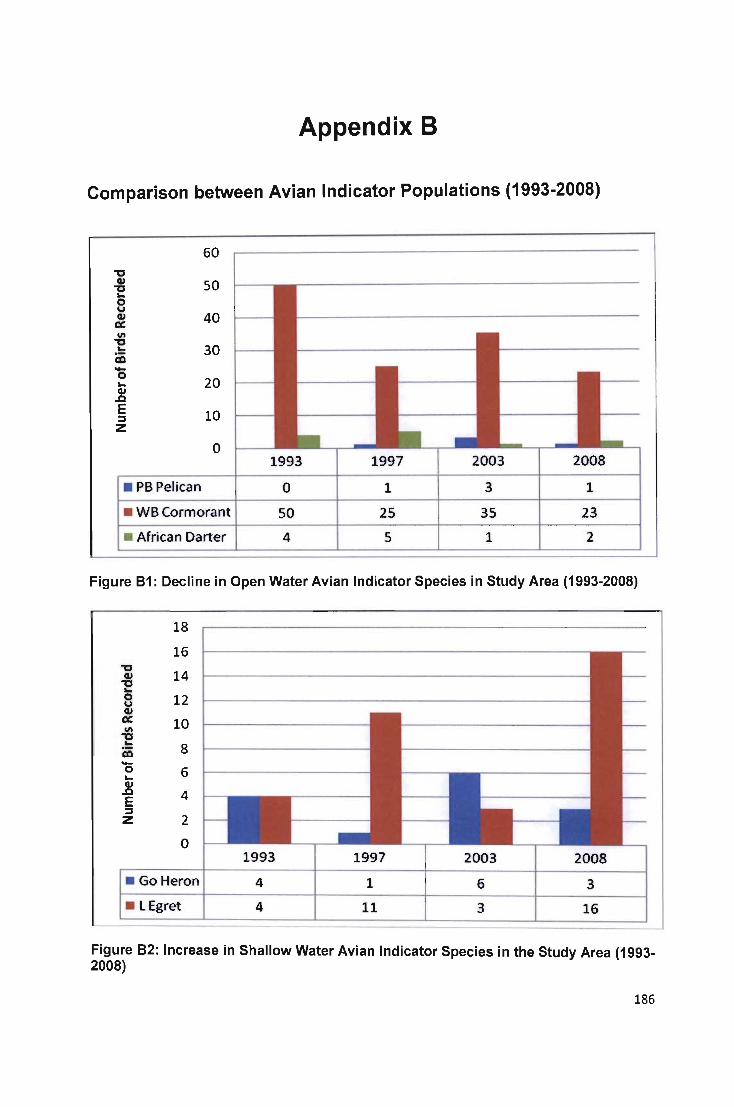
Appendix B
Comparison between Avian Indicator Populations (1993-2008)
60 "0
CLI 50 "0 ~
8 CLI 40 cr:: VI "0
30 ~
iii -0 20 ~
CLI .Q
E 10 :;, z
0 1993 1997 2003 2008
• PB Pelican 0 1 3 1
• WB Cormorant 50 25 35 23
• African Darter 4 5 1 2
Figure 81: Decline in Open Water Avian Indicator Species in Study Area (1993-2008)
18
16 "0
14 CLI "0 ~
0 12 u CLI cr:: 10 VI "0 ~
8 iii '0 6 ~
CLI .Q 4 E :;, z 2
0 1993 1997 2003 2008
• Go Heron 4 1 6 3
. lEgret 4 11 3 16
Figure 82: Increase in Shallow Water Avian Indicator Species in the Study Area (1993-2008)
186
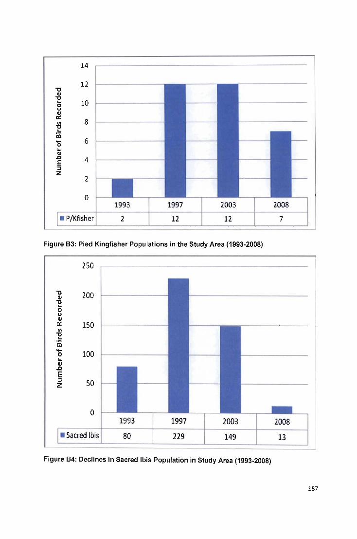
14
12 "t:I QI
"t:I ... 10 0 u QI a:
8 III "t:I ... &il .... 6 0 ... QI
.Q 4 E :J Z
2
0 1993 1997 2003 2008
• P/Kfisher 2 12 12 7
Figure 83: Pied Kingfisher Populations in the Study Area (1993-2008)
250
"t:I 200 OJ "t:I ... 0 u OJ ex: 150 III
"t:I ... ~ ....
100 0 ... OJ .a E :J SO 2
o 1993 1997 2003 2008
• Sacred Ibis 80 229 149 13
Figure 84: Declines in Sacred Ibis Population in Study Area (1993-2008)
187

18
16 "0 0.1 14 "0 .. 0
12 u 0.1 ~ \I) 10 "0 .. en 8 '0 ..
6 0.1 .c E
4 j
z 2
0 1993 1997 2003 2008
• BS Plover 2 16 3 17
Figure B5: Increase in Blacksmith Plover Population in the Study Area (1993-2008)
25
"0 20 0.1
"0 .. 0 u 0.1 15 ~ \I)
"0 .. iii 10 -0 .. 0.1 5 .c E :::s Z
0 1991 1997 2003 2008
• Water Dikkop 2 16 3 17
• PHeron 3 3 5 3
• Woolly-Necked Stork 2 1 22 3
Figure B6: Increase in Vegetated Areas Indicator Species in the Study Area (1993-
2008)
188
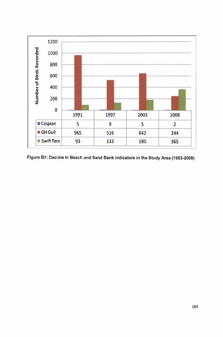
1200 '0 CI.I 1000 '0 "" 0 u CI.I 800 a:: !II '0
600 "" .-al ~
0 400 "" CI.I
.ll E 200 ~ z
a 1991 1997 2003 2008
• Caspian 5 9 5 2
• GH Gull 965 526 642 244
• Swift Tern 93 133 180 365
Figure B7: Decline in Beach and Sand Bank Indicators in the Study Area (1993-2008)
189

Appendix C
Wetland Avian Indicator Species
The figures below represent the number of birds of each indicator species counted in the
vicinity of the Mgeni Estuary and Beachwood Mangrove Swamps during CWAC Wetland
Bird Surveys between 1993 and 2008.
60 ... C IV ~
50 0 E ~
0 U '0 40 QI t;'O IV QI QI'O ~ ~ 30 co 0 • u ! QI :cD:: ~ 20 '0 ~
QI .Q 10 E :J Z
0
1993 1997 2000 2003 2005 2007 2008 Time Period
Figure C1: CWAC Wetland Avian Census Data for WB Cormorant (1993-2008
Figure C2: CWAC Wetland Avian Cencus Data for Sacred Ibis (1993-2008)
190

7
"0 Q/ 6 "0 ... 0 u Q/ 5 a: c: 0 ... Q/ 4 ::z::
.z= .. • !!! 3 0 C)
'0 2 ... Q/
..Q
E 1 ::s Z
0
1993 1997 2000 2003 2005 2007 2008
Time Period
Figure C3: CWAC Wetland Avian Census Data for Goliath Heron (1993-2008)
20
18 "0 Q/ "0 16 ... 0 u
14 Q/ a: .. Q/ 12 ... til) W Q/ 10 'E :::; 8 .... 0 ... 6 Q/
..Q
E 4 ::s z 2
0
1993 1997 2000 2003 2005 2007 2008 Time Period
Figure C4: CWAC Wetland Avian Census Data for Little Egret (1993-2008)
191
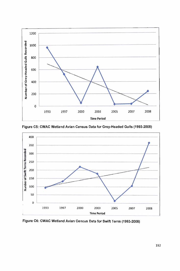
1200
'tJ CII
1000 'tJ ... 0 u CII a:: .!!! 800 '3
" 'tJ CII 'tJ 600 ~ CII
::.c . > CII ... " 400 .... 0 ... CII ~
E 200 :s z
0
1993 1997 2000 2003 2005 2007 2008
Time Period
Figure C5: CWAC Wetland Avian Census Data for Grey-Headed Gulls (1993-2008)
400
350 'tJ CII 'tJ 300 ... 0 u CII a:: 250 VI c ... CII I- 200 ... :t: ~ VI .... 150 0 ... CII ~
E 100 ::I Z
SO
0
1993 1997 2000 2003 2005 2007 2008
TIme Period
Figure C6: CWAC Wetland Avian Cencus Data for Swift Terns (1993-2008)
192
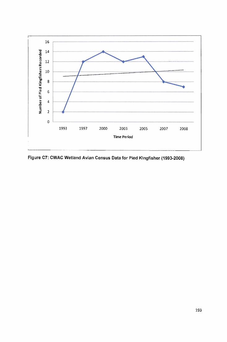
16
"tI 14 CII "tI ... 0 u 12 cu a:: <II ... CII 10 .s:. <II
'to 8 c
~ "tI CII 6 a: .... 0 ...
4 CII .a E ::J 2 z
0
1993 1997 2000 2003 2005 2007 2008
Time Period
Figure C7: CWAC Wetland Avian Census Data for Pied Kingfisher (1993-2008)
193

Orientation Map
N
Free State
l.!ESOTHO
Appendix D
Mpumalanga
Indian Ocean
Legend
• Research Area o MajorTowns
- National Routes Local Municipalities
District Municipalities Eastern Cape
eo eo 100 120 140 km
Free State Mpumalanga LESOTHO
MOZAMBIQUES
SWAZILAND - - - -194
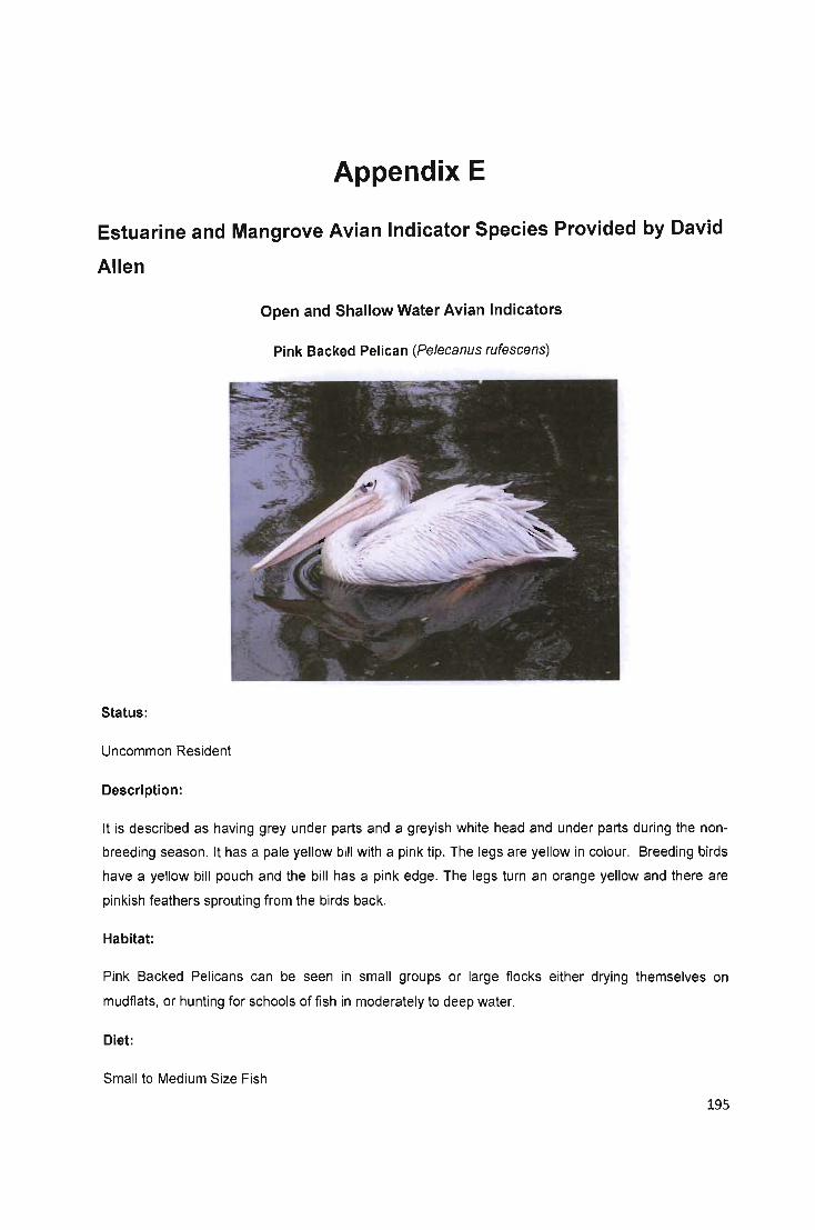
Appendix E
Estuarine and Mangrove Avian Indicator Species Provided by David
Allen
Open and Shallow Water Avian Indicators
Pink Backed Pelican (Pelecanus rufescens)
Status:
Uncommon Resident
Description:
It is described as having grey under parts and a greyish white head and under parts during the non
breeding season. It has a pale yellow bill with a pink tip. The legs are yellow in colour. Breeding birds
have a yellow bill pouch and the bill has a pink edge. The legs turn an orange yellow and there are
pinkish feathers sprouting from the birds back.
Habitat:
Pink Backed Pelicans can be seen in small groups or large flocks either drying themselves on
mudflats, or hunting for schools of fish in moderately to deep water.
Diet:
Small to Medium Size Fish
195
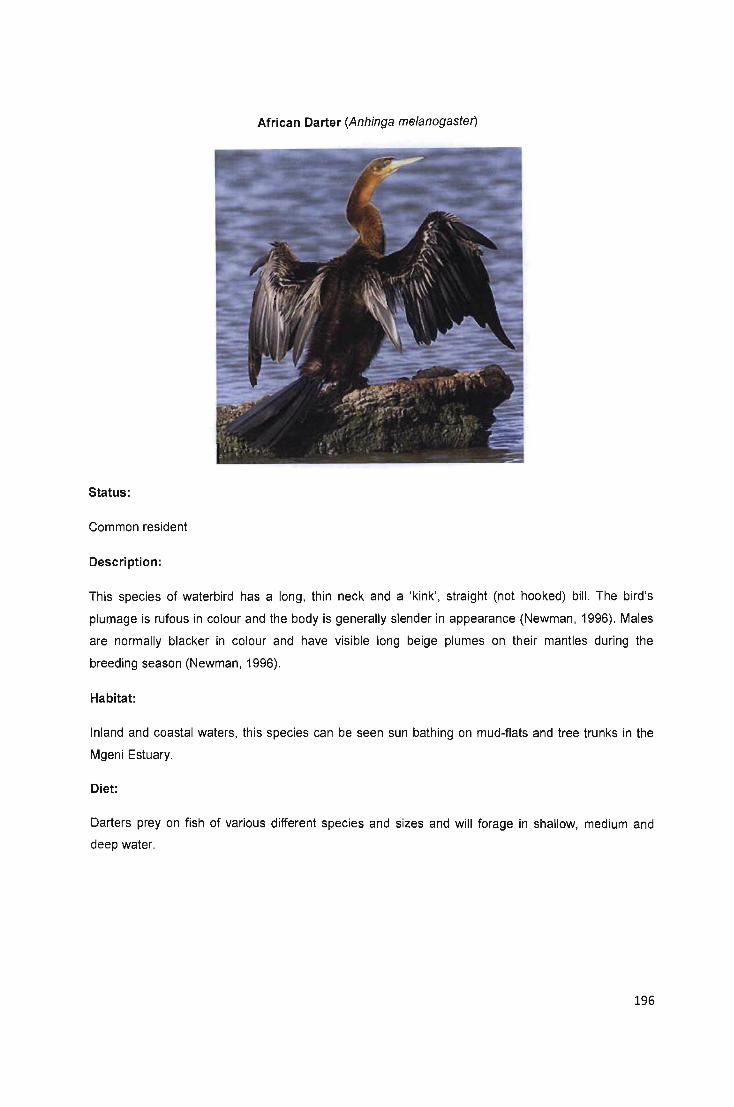
African Darter (Anhinga melanogaster)
Status:
Common resident
Description:
This species of waterbird has a long, thin neck and a 'kink', straight (not hooked) bill . The bird's
plumage is rufous in colour and the body is generally slender in appearance (Newman, 1996). Males
are normally blacker in colour and have visible long beige plumes on their mantles during the
breeding season (Newman, 1996).
Habitat:
Inland and coastal waters, this species can be seen sun bathing on mud-flats and tree trunks in the
Mgeni Estuary.
Diet:
Darters prey on fish of various different species and sizes and will forage in shallow, medium and
deep water.
196
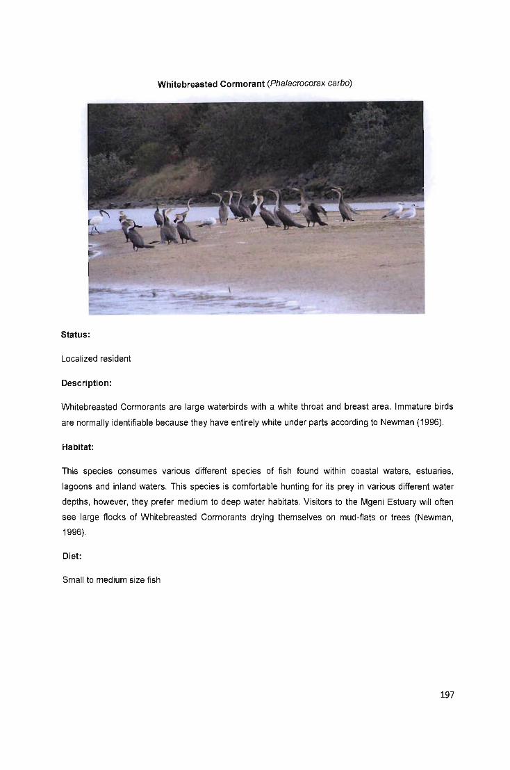
Whitebreasted Cormorant (Phalacrocorax carbo)
Status:
Localized resident
Description:
Whitebreasted Cormorants are large waterbirds with a white throat and breast area. Immature birds
are normally identifiable because they have entirely white under parts according to Newman (1996).
Habitat:
This species consumes various different species of fish found within coastal waters, estuaries,
lagoons and inland waters. This species is comfortable hunting for its prey in various different water
depths, however, they prefer medium to deep water habitats. Visitors to the Mgeni Estuary will often
see large flocks of Whitebreasted Cormorants drying themselves on mud-flats or trees (Newman,
1996).
Diet:
Small to medium size fish
197

Goliath Heron (Ardea goliath)
Status:
Common Resident
Description:
It is a robust bird with slated-grey upperparts and rich rufous under parts (Newman, 1996)
Habitat:
This species of heron can be found near rivers, lakes, pans and estuaries.
Diet:
The species will also move slowly along the shoreline hunting for frogs, mice, rats, snakes and other
vertebrates. The Goliath Heron can frequently seen hunting in the deeper water of the Mgeni Estuary,
standing motionless for long period waiting for its prey to come into range of its long, sharp bill
(Newman, 1996).
Important Fact:
This species of heron is the largest of all herons.
198

Little Egret (Egretta garzetta)
Status:
Common Resident
Description:
This species of egret has a larger, longer neck than other species and the bill and legs are longer and
black. The feet are yellow. The species can be identified easily by its unmistakable white head plumes
(Newman, 1996).
Habitat:
Inland waters, estuaries and coastal pools (Newman, 1996).
Diet:
This species is a common resident often seen standing motionless in the shallows or walk forward
slowly, stealthily hunting for small fish and aquatic and terrestrial invertebrates.
199
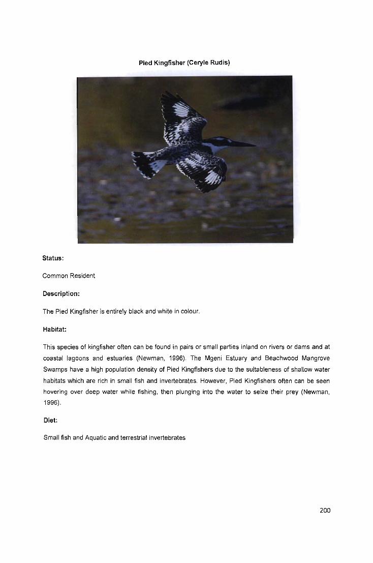
Pied Kingfisher (Ceryle Rudis)
Status:
Common Resident
Description:
The Pied Kingfisher is entirely black and white in colour.
Habitat:
This species of kingfisher often can be found in pairs or small parties inland on rivers or dams and at
coastal lagoons and estuaries (Newman, 1996). The Mgeni Estuary and Beachwood Mangrove
Swamps have a high population density of Pied Kingfishers due to the suitableness of shallow water
habitats which are rich in small fish and invertebrates. However, Pied Kingfishers often can be seen
hovering over deep water while fishing, then plunging into the water to seize their prey (Newman,
1996).
Diet:
Small fish and Aquatic and terrestrial invertebrates
200
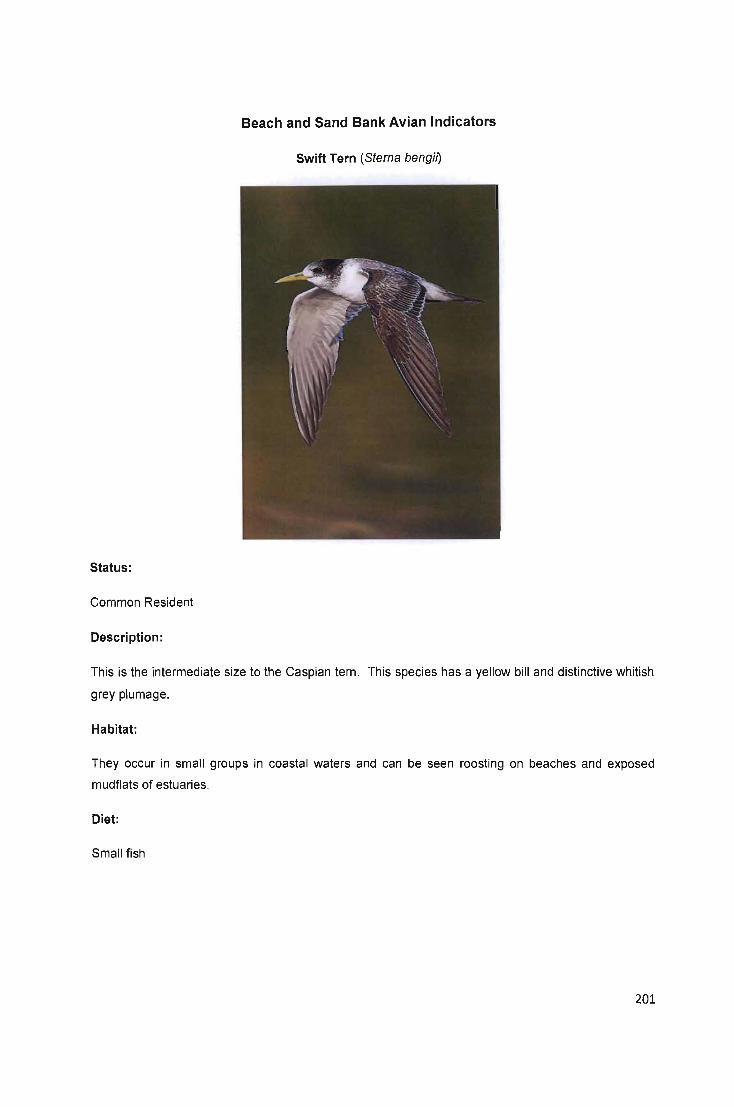
Beach and Sand Bank Avian Indicators
Swift Tern (Sterna bengiJ)
Status:
Common Resident
Description:
This is the intermediate size to the Caspian tern . This species has a yellow bill and distinctive whitish
grey plumage.
Habitat:
They occur in small groups in coastal waters and can be seen roosting on beaches and exposed
mudflats of estuaries.
Diet:
Small fish
201
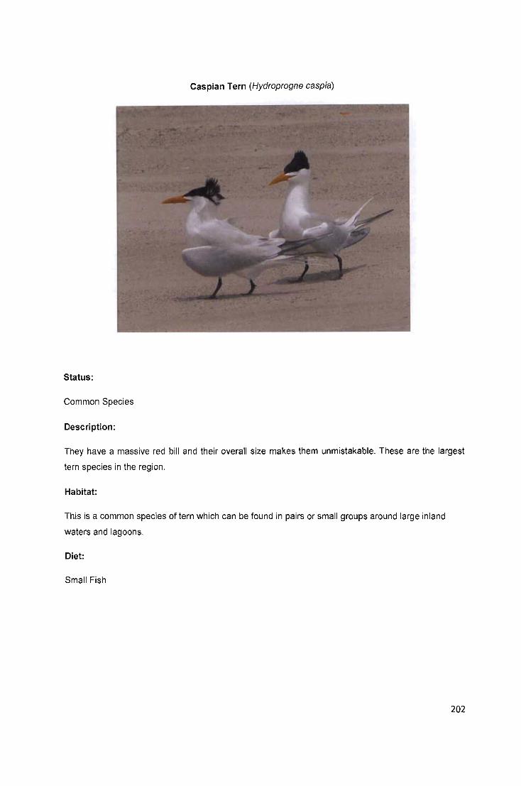
Caspian Tern (Hydroprogne caspia)
Status:
Common Species
Description:
They have a massive red bill and their overall size makes them unmistakable. These are the largest
tern species in the region.
Habitat:
This is a common species of tern which can be found in pairs or small groups around large inland
waters and lagoons.
Diet:
Small Fish
202

Grey Headed Gull (Larus cirrocephalus)
Status:
Common Resident
Description:
Distinctive grey hood and the bill , legs and feet are bright red. The eyes are yellowish white with a red
ring around them.
Habitat:
Coastal habitats and inland water sources such as dams, rivers and lakes.
Diet:
Aquatic and terrestrial invertebrates, frogs and fish
203
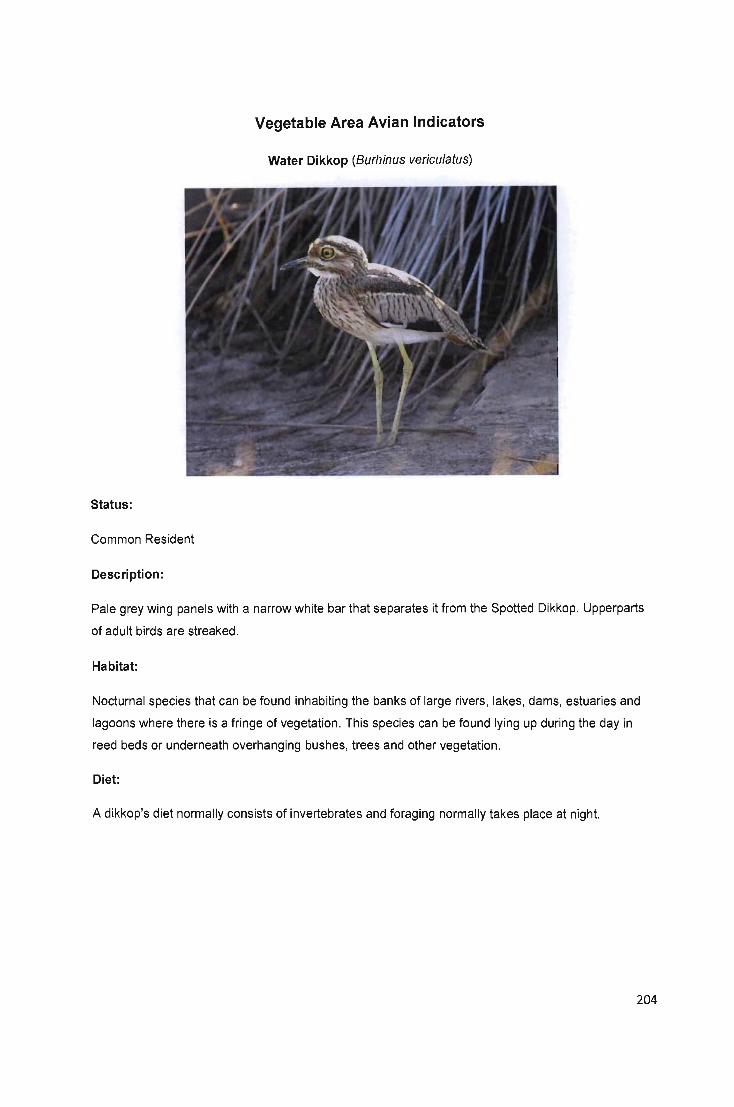
Vegetable Area Avian Indicators
Water Dikkop (Burhinus vericulatus)
Status:
Common Resident
Description:
Pale grey wing panels with a narrow white bar that separates it from the Spotted Dikkop. Upperparts
of adult birds are streaked.
Habitat:
Nocturnal species that can be found inhabiting the banks of large rivers , lakes, dams, estuaries and
lagoons where there is a fringe of vegetation . This species can be found lying up during the day in
reed beds or underneath overhanging bushes, trees and other vegetation.
Diet:
A dikkop's diet normally consists of invertebrates and foraging normally takes place at night.
204
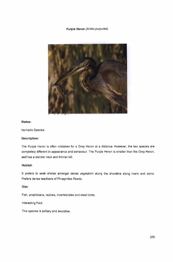
Purple Heron (Ardea purpurea)
Status:
Nomadic Species
Description:
The Purple Heron is often mistaken for a Grey Heron at a distance. However, the two species are
completely different in appearance and behaviour. The Purple Heron is smaller than the Grey Heron,
and has a slender neck and thinner bill.
Habitat:
It prefers to seek shelter amongst dense vegetation along the shoreline along rivers and dams.
Prefers dense reed beds of Phragmites Reeds.
Diet:
Fish, amphibians, reptiles, invertebrates and small birds.
Interesting Fact:
This species is solitary and secretive.
205
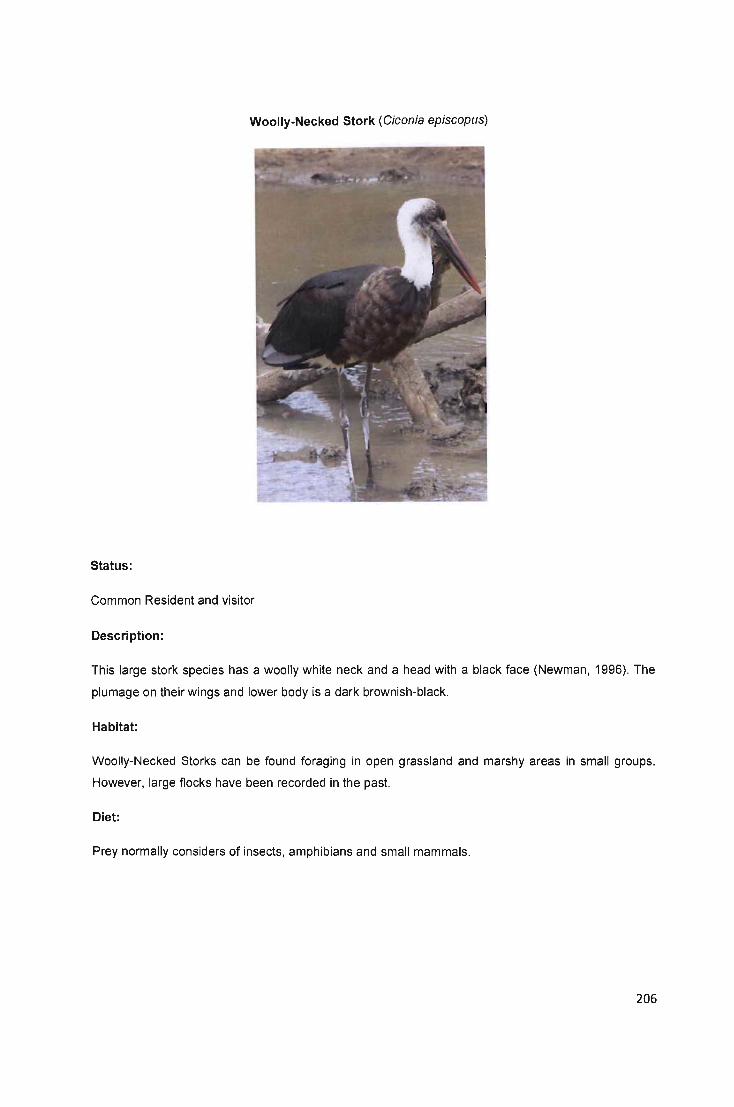
Woolly-Necked Stork (Ciconia episcopus)
Status:
Common Resident and visitor
Description:
This large stork species has a woolly white neck and a head with a black face (Newman, 1996). The
plumage on their wings and lower body is a dark brownish-black.
Habitat:
Woolly-Necked Storks can be found foraging in open grassland and marshy areas in small groups.
However, large flocks have been recorded in the past.
Diet:
Prey normally considers of insects, amphibians and small mammals.
206
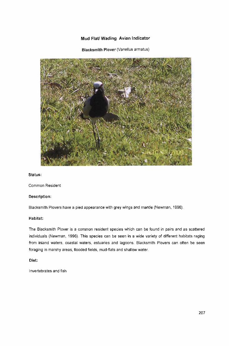
Mud Flat! Wading Avian Indicator
Blacksmith Plover (Vanellus armatus)
Status:
Common Resident
Description:
Blacksmith Plovers have a pied appearance with grey wings and mantle (Newman, 1996).
Habitat:
The Blacksmith Plover is a common resident species which can be found in pairs and as scattered
individuals (Newman, 1996). This species can be seen in a wide variety of different habitats raging
from inland waters, coastal waters, estuaries and lagoons. Blacksmith Plovers can often be seen
foraging in marshy areas, flooded fields, mud-flats and shallow water.
Diet:
Invertebrates and fish
207

Sanderling (Calidris alba)
Status:
Common Migrant
Description:
This is a small shorebird which is white in appearance with darker shoulder-patches. It has a short,
thick bill which is used to probe the mud for worms and other organisms.
Habitat:
Found in estuarine habitats, in particular along the shoreline and on mud-flats. Sanderlings run along
the water's edge at speed and feeding where the waves and water recede which is a characteristic of
this species. A regular visitor to the Mgeni Estuary, the Sanderling is one of the most common
summer migrants to Kwa-Zulu Natal's shores.
Diet:
Invertebrates
208
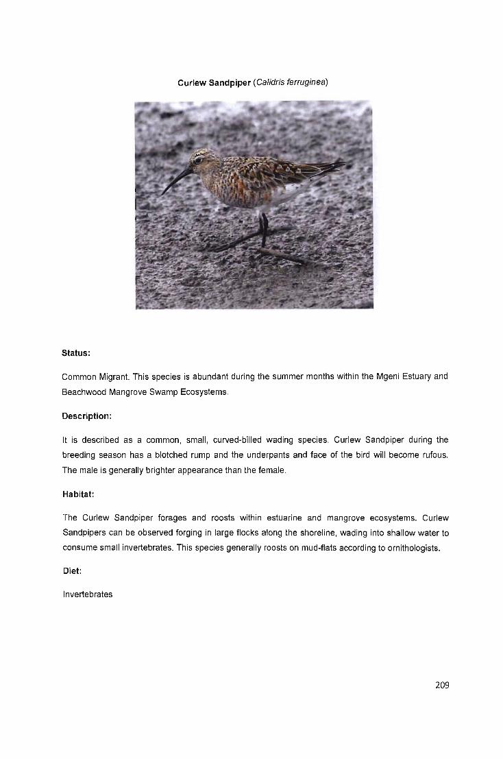
Curlew Sandpiper (Calidris ferruginea)
Status:
Common Migrant. This species is abundant during the summer months within the Mgeni Estuary and
Beachwood Mangrove Swamp Ecosystems.
Description:
It is described as a common, small, curved-billed wading species. Curlew Sandpiper during the
breeding season has a blotched rump and the underpants and face of the bird will become rufous.
The male is generally brighter appearance than the female.
Habitat:
The Curlew Sandpiper forages and roosts within estuarine and mangrove ecosystems. Curlew
Sandpipers can be observed forging in large flocks along the shoreline, wading into shallow water to
consume small invertebrates. This species generally roosts on mud-flats according to ornithologists.
Diet:
Invertebrates
209
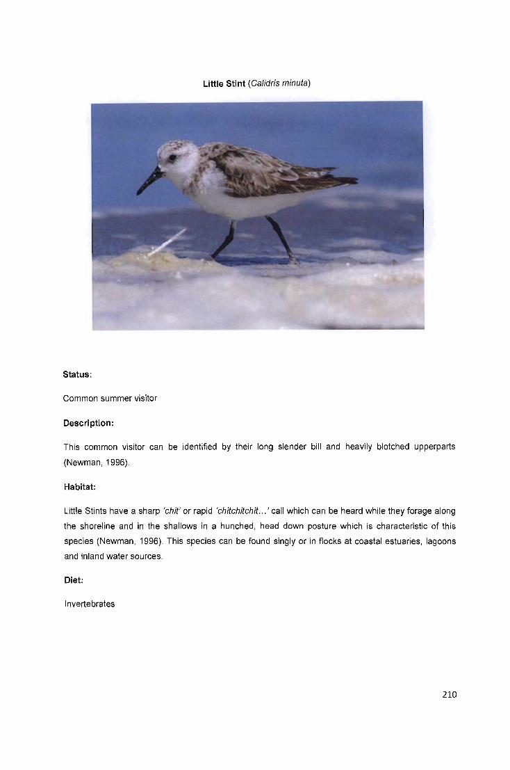
Little Stint (Calidris minuta)
Status:
Common summer visitor
Description:
This common visitor can be identified by their long slender bill and heavily blotched upperparts
(Newman, 1996).
Habitat:
Little Stints have a sharp 'chit' or rapid 'chitchitchit ... ' call which can be heard while they forage along
the shoreline and in the shallows in a hunched, head down posture which is characteristic of this
species (Newman, 1996). This species can be found singly or in flocks at coastal estuaries, lagoons
and inland water sources.
Diet:
Invertebrates
210
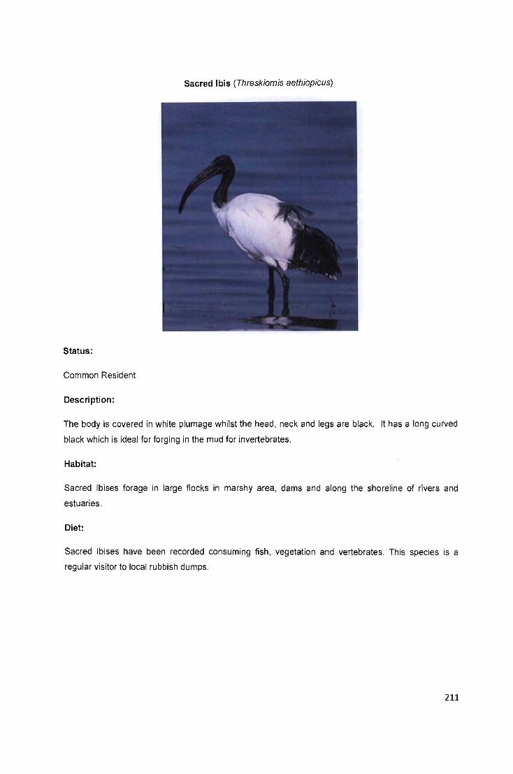
Sacred Ibis (Threskiornis aethiopicus)
Status:
Common Resident
Description:
The body is covered in white plumage whilst the head , neck and legs are black. It has a long curved
black which is ideal for forging in the mud for invertebrates.
Habitat:
Sacred Ibises forage in large flocks in marshy area, dams and along the shoreline of rivers and
estuaries.
Diet:
Sacred Ibises have been recorded consuming fish , vegetation and vertebrates. This species is a
regular visitor to local rubbish dumps.
211
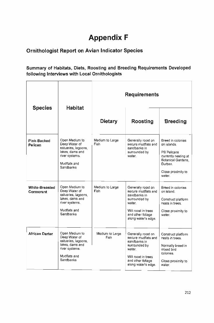
Appendix F
Ornithologist Report on Avian Indicator Species
Summary of Habitats, Diets, Roosting and Breeding Requirements Developed following Interviews with Local Ornithologists
Requirements
Species Habitat
Dietary Roosting Breeding
Pink-Backed Open Medium to Medium to Large Generally roost on Breed in colonies Pelican Deep Water of Fish secure mudflats and on islands.
estuaries, lagoons, sandbanks in lakes, dams and surrounded by PB Pelicans river systems. water. currently nesting at
Botanical Gardens, Mudflats and Durban. Sandbanks
Close proximity to water.
White-Breasted Open Medium to Medium to Large Generally roost on Breed in colonies Cormorant Deep Water of Fish secure mudflats and on island.
estuaries, lagoons, sandbanks in lakes, dams and surrounded by Construct platform river systems. water. nests in trees.
Mudflats and Will roost in trees Close proximity to Sandbanks and other foliage water.
along water's edge.
African Darter Open Medium to Medium to Large Generally roost on Construct platform Deep Water of Fish secure mudflats and nests in trees. estuaries, lagoons, sandbanks in lakes, dams and surrounded by Normally breed in river systems. water. mixed bird
colonies. Mudflats and Will roost in trees Sandbanks and other foliage Close proximity to
along water's edge. water.
212
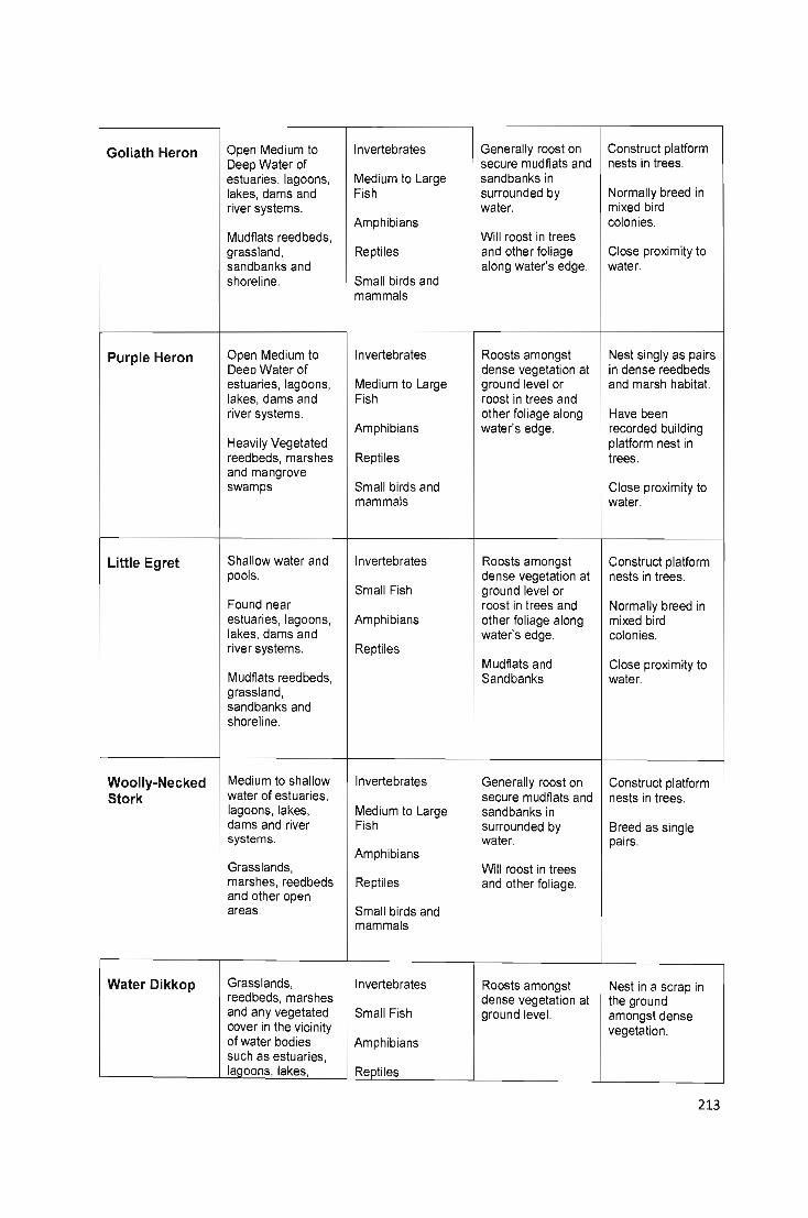
Goliath Heron Open Medium to Invertebrates Generally roost on Construct platform Deep Water of secure mudflats and nests in trees. estuaries, lagoons, Medium to Large sandbanks in lakes, dams and Fish surrounded by Normally breed in river systems. water. mixed bird
Amphibians colonies. Mudflats reedbeds, Will roost in trees grassland, Reptiles and other foliage Close proximity to sandbanks and along water's edge. water. shoreline. Small birds and
mammals
Purple Heron Open Medium to Invertebrates Roosts amongst Nest singly as pairs Deep Water of dense vegetation at in dense reed beds estuaries, lagoons, Medium to Large ground level or and marsh habitat. lakes, dams and Fish roost in trees and river systems. other foliage along Have been
Amphibians water's edge. recorded building Heavily Vegetated platform nest in reed beds, marshes Reptiles trees. and mangrove swamps Small birds and Close proximity to
mammals water.
Little Egret Shallow water and Invertebrates Roosts amongst Construct platform pools. dense vegetation at nests in trees.
Small Fish ground level or Found near roost in trees and Normally breed in estuaries, lagoons, Amphibians other foliage along mixed bird lakes, dams and water's edge. colonies. river systems. Reptiles
Mudflats and Close proximity to Mudflats reedbeds, Sandbanks water. grassland, sandbanks and shoreline.
Woolly-Necked Medium to shallow Invertebrates Generally roost on Construct platform Stork water of estuaries, secure mudflats and nests in trees.
lagoons, lakes, Medium to Large sandbanks in dams and river Fish surrounded by Breed as single systems. water. pairs.
Amphibians Grasslands, Will roost in trees marshes, reed beds Reptiles and other foliage. and other open areas. Small birds and
mammals
Water Dikkop Grasslands, Invertebrates Roosts amongst Nest in a scrap in reed beds, marshes dense vegetation at the ground and any vegetated Small Fish ground level. amongst dense cover in the vicinity vegetation. of water bodies Amphibians such as estuaries, lagoons, lakes, R~tiles
213
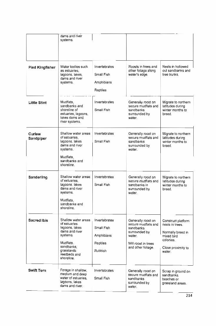
dams and river systems.
Pied Kingfisher Water bodies such Invertebrates Roosts in trees and Nests in hollowed as estuaries, other foliage along out sandbanks and lagoons, lakes, Small Fish water's edge. tree trunks. dams and river systems. Amphibians
Reptiles
Little Stint Mudflats, Invertebrates Generally roost on Migrate to northern sandbanks and secure mudflats and latitudes during shoreline of Small Fish sandbanks winter months to estuaries, lagoons, surrounded by breed. lakes dams and water. river systems.
Curlew Shallow water areas Invertebrates Generally roost on Migrate to northern Sandpiper of estuaries, secure mudflats and latitudes during
lagoons, lakes Small Fish sandbanks winter months to dams and river surrounded by breed. systems. water.
Mudflats, sandbanks and shoreline.
Sanderling Shallow water areas Invertebrates Generally roost on Migrate to northern of estuaries, secure mudflats and latitudes during lagoons, lakes Small Fish sandbanks in winter months to dams and river surrounded by breed. systems. water.
Mudflats, sandbanks and shoreline.
Sacred Ibis Shallow water areas Invertebrates Generally roost on Construct platform of estuaries, secure mudflats and nests in trees. lagoons, lakes Small Fish sandbanks dams and river surrounded by Normally breed in systems. Amphibians water. mixed bird
colonies. Mudflats, Reptiles Will roost in trees sandbanks, and other foliage. Close proximity to grasslands Rubbish water. reed beds and shoreline.
Swift Tern Forage in shallow, Invertebrates Generally roost on Scrap in ground on medium and deep secure mudflats and sandbanks, water of estuaries, Small Fish sandbanks beaches or lagoons, lakes surrounded by grassland areas. dams and river. water.
214
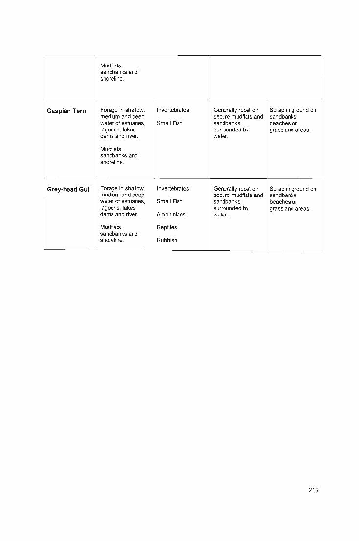
Mudflats, sandbanks and shoreline.
Caspian Tern Forage in shallow, Invertebrates Generally roost on Scrap in ground on medium and deep secure mudflats and sandbanks, water of estuaries, Small Fish sandbanks beaches or lagoons, lakes surrounded by grassland areas. dams and river. water.
Mudflats, sandbanks and shoreline.
Grey-head Gull Forage in shallow, Invertebrates Generally roost on Scrap in ground on medium and deep secure mudflats and sandbanks, water of estuaries, Small Fish sandbanks beaches or lagoons, lakes surrounded by grassland areas. dams and river. Amphibians water.
Mudflats, Reptiles sandbanks and shoreline. Rubbish
215

Appendix G
Land Cover Classes Classification System
Land Cover Classes A Brief Description of Land
Cover
Indigenous and Woodland Tree Canopy cover between 30-
Invasive Forest and 60%
Woodland Coastal Forest Tree Canopy cover between 60-
100%
Mangrove Forest Vegetation covers between 70-
100%. Majority of vegetation cover
consisting of mangrove tree
species.
Island Mangrove Vegetation Vegetation covers between 40-
60%. Majority of vegetation cover
consisting of mangrove tree
species.
Grasslands (Natural Man-Managed Grass Area Open artificial or natural grass
and Artificial) covered area maintained by local
municipality or other affiliated
groups.
Grassland Scrubland Mixture of indigenous vegetation
and grass cover.
Wetlands/Reedbeds Reedbeds and Marsh Vegetation covers between 70-
100%. Majority of vegetation cover
consisting of indigenous or
invasive reed species.
Reedbeds and Grassland Vegetation covers between 30-
40%. Mixture of grass, sedge and
216

other vegetation species present.
Coastal Vegetation Dune Vegetation Dune adapted vegetation covers
between 60-1 00%.
Water Bodies Shallow Water Water of a depth less than 1 meter
Open Water Water of a depth greater than 1
meter
Conservation Development Areas of roads and buildings
Managed Area managed by KZN Ezembelo
Wildlife.
Other Land Covers Exposed Mudflats Areas of exposed mud and sand
within the vicinity of the river
channel or estuary mouth.
Sandbanks Sand deposited by river and sea
currents at mouth of estuary.
Salt Marsh Bear or partly vegetated ground
highly saline in nature.
Beach Open area of sand used for
recreational purposes.
217

Appendix H
CWAC Data Permission Request Form
~ ~ COORDINATED WATERBIRD COUNTS
CWAC Data Request Sheet
biodiversity institute
SAN B I
Animal Demography Unit
Department of Zoology
University of Cape Town
Rondebosch 7701
South Africa
www.adu.org.za
Tel. +27 (0)21 6504698
Fax +27 (0)21 6503434
Please provide the relevant information to allow me to process your data request effectively. You
can send the form back to the CWAC project coordinator: [email protected]. Upon
receiving the request I will be in touch regarding availability, permission, conditions of data use and
costs if applicable.
Date: 01/06/2009
Name: Andrew Batho
Company / Affiliation: Private use (Masters Research Paper)
Postal address: 7 Barn Place Westville Durban 3630
Email address:[email protected]
218
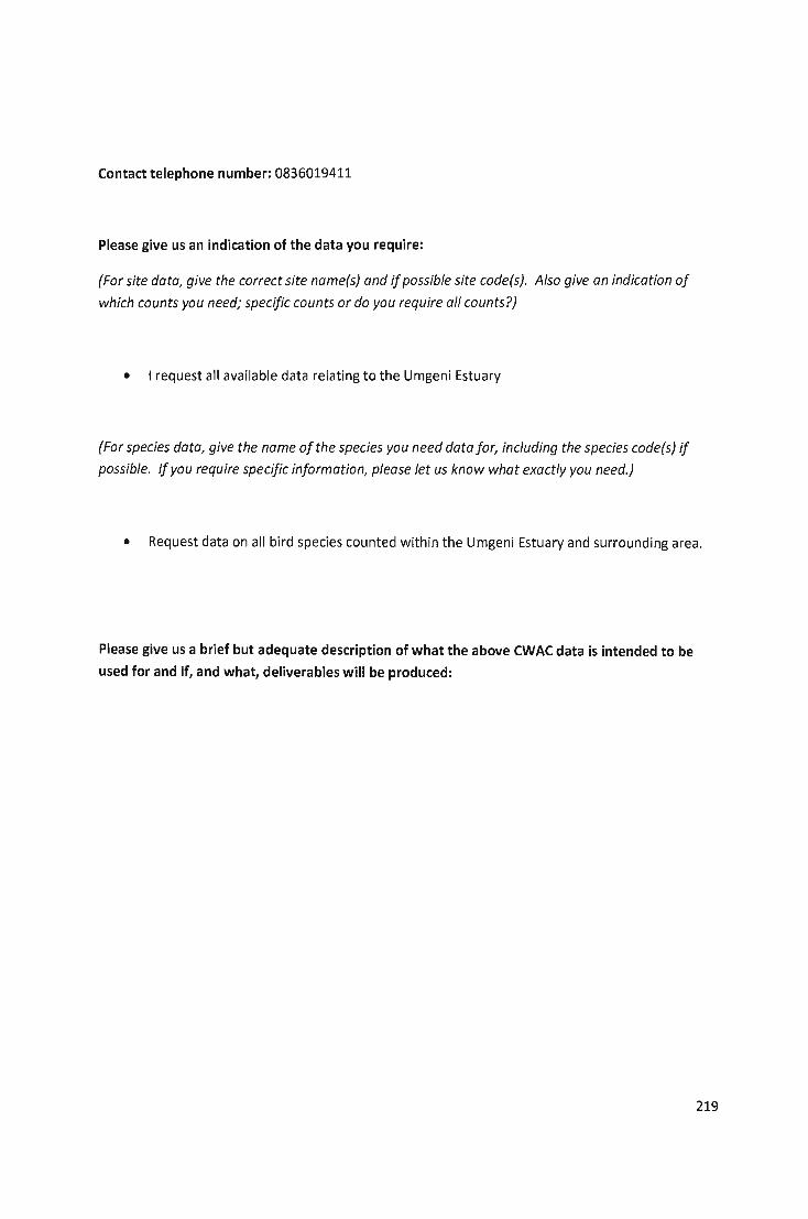
Contact telephone number: 0836019411
Please give us an indication of the data you require:
(For site data, give the correct site name(s) and if possible site code(s). Also give an indication of which counts you need; specific counts or do you require all counts?)
• I request all available data relating to the Umgeni Estuary
(For species data, give the name of the species you need data for, including the species code(s) if possible. If you require specific information, please let us know what exactly you need.)
• Request data on all bird species counted within the Umgeni Estuary and surrounding area.
Please give us a brief but adequate description of what the above CWAC data is intended to be
used for and if, and what, deliverables will be produced:
219
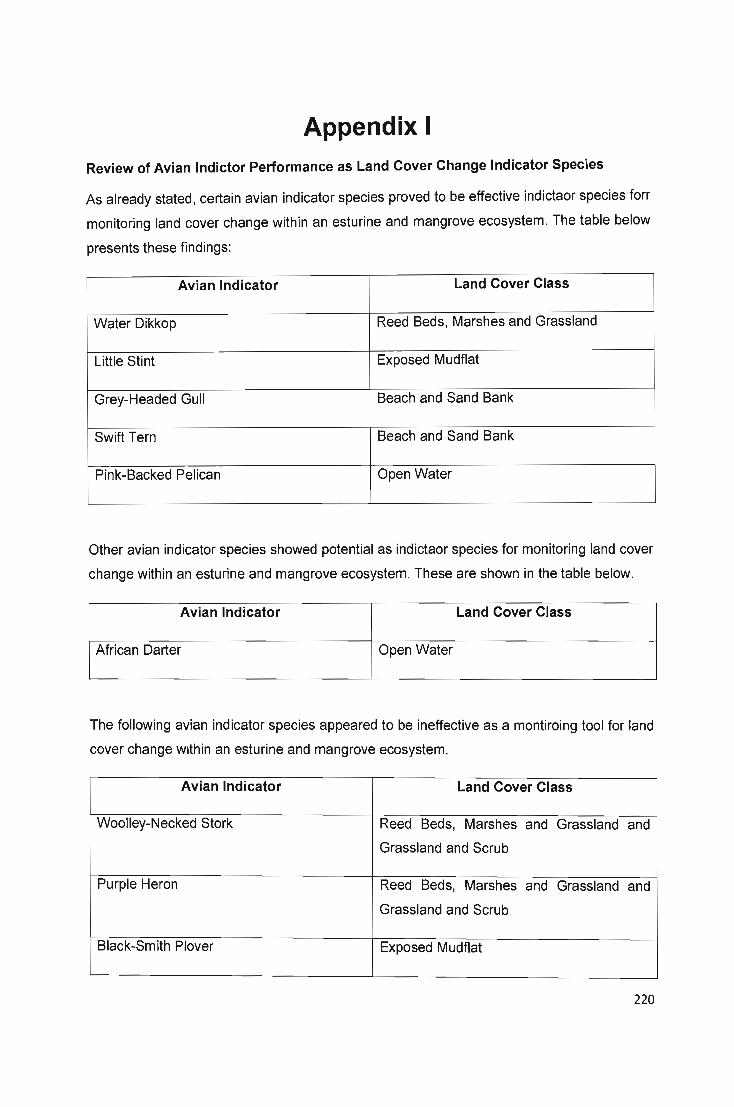
Appendix I Review of Avian Indictor Performance as Land Cover Change Indicator Species
As already stated, certain avian indicator species proved to be effective indictaor species forr
monitoring land cover change within an esturine and mangrove ecosystem. The table below
presents these findings:
Avian Indicator Land Cover Class
Water Dikkop Reed Beds, Marshes and Grassland
Little Stint Exposed Mudflat
Grey-Headed Gull Beach and Sand Bank
Swift Tern Beach and Sand Bank
Pink-Backed Pelican Open Water
Other avian indicator species showed potential as indictaor species for monitoring land cover
change within an esturine and mangrove ecosystem. These are shown in the table below.
Avian Indicator Land Cover Class
African Darter Open Water
The following avian indicator species appeared to be ineffective as a montiroing tool for land
cover change within an esturine and mangrove ecosystem.
Avian Indicator Land Cover Class
Woolley-Necked Stork Reed Beds, Marshes and Grassland and
Grassland and Scrub
Purple Heron Reed Beds, Marshes and Grassland and
Grassland and Scrub
Black-Smith Plover Exposed Mudflat
220

Caspian Tern Beach and Sand Bank
Sanderling Exposed Mudflat
Sacred Ibis Exposed Mudflat
221
Appendix J
Criteria Utilised for Selecting Avian Indicators
The Little Stint is the smallest wading bird species was considered ideal as a mudflat
indicator species because it is adapted to hunting for its prey on exposed mudflats, and is a
regular visitor to the Mgeni Estuary. The Little Stint has small legs which prevent it wading
into the deeper water channels and estuary itself, plus it has a small beak which cannot
probe far beneath the surface of the mudflats. Little Stints rely entirely upon mudflats as a
source of nutrients (Velasquez and Hockey, 1992). Other mudflat zone indicator species
such as Curlews and Sandpipers, are recognisable because of their larger body size
correlating with a larger beak and longer legs adapted to wading into deeper water as
mentioned previously. The longer bill provides these wading species with the ability to probe
deeper into mudflats and sandbanks to catch prey. Meanwhile, Black-Smith Plovers are
exclusively a visual foraging bird species. Black-Smith Plovers have a small beak designed
for shallow probing and securing prey on the surface of exposed mudflats (Velasquez and
Hockey, 1992). Sacred Ibis are described as a generalist species because of their ability to
forage in a variety of different habitats ranging from the exposed mudflats of an estuarine
ecosystem to man-made waste disposal sites further inland. However, the researcher
observed ibis congregating and foraging on exposed mudflats and sandbanks within the
Mgeni Estuary and Beachwood Mangrove Swamp study area on a regular basis throughout
the cause of the study. Therefore, based on the information provided by avian literature and
ornithologists, and the researchers own observations, the Little Stint, Curlew Sandpiper,
Sanderlings, Sacred Ibis and Black-Smith Plover were selected as an indicator species for
mudflat habitats that are found along the main Mgeni Estuary waterways and channel.
The researcher selected African Darter, White-Breasted Cormorant and the Pink-Backed
Pelican as medium to deep water habitat indicators based on the information provided by
avian literature and advice provided by ornithologists. These sources indicated that
cormorants, darters and pelicans forage exclusively in open , deep water habitats such as the
channels of rivers, estuaries and lagoons (Velasquez and Hockey, 1992). Pelican species
forage in open water of the estuary channels and inlets and generally consume prey that has
been caught just below the water's surface. Cormorants and darters forage for a variety of
222

different fish species by diving beneath the water's surface and hunting amongst submerged
logs, water vegetation and other obstacles below the surface.
Herons, storks and egrets have adopted a wading foraging technique. Goliath Herons and
Little Egrets are ideally adapted to their chosen foraging habitats and prey species with long
legs to carry them above the water quickly and efficiently, a long snake-like flexible neck and
a robust beak to grasp and restrain struggling prey (Allen, 2008). White Egret tends to forage
in shallow water of an average depth of 100mm, while Goliath Heron can be found foraging
in water of a depth of 325mm (Velasquez and Hockey, 1992}.Goliath Herons and Little
Egrets are often seen moving steadily through shallow and medium deep water along the
estuarine shoreline, moving their feet around amongst the mud and vegetation of the estuary
bottom to scare fish, amphibians and other prey out into the open. When the bird observes
movement below the water surface, it will plunge its beak into to water to catch the prey
item. Herons and egrets have perfected a second foraging technique that helps conserve
value energy. Little Egrets will often standing motionless, practising a 'sit-and-wait' strategy
to catch unsuspecting prey along the water's edge (Velasquez and Hockey, 1992). These
foraging techniques unique to the heron, stork and egret species and the reliance on water
habitats for foraging, provided the researcher with adequate empathises for the selection of
the Goliath Heron and Little Egret as Medium and Shallow Water Zone Indicator Species.
Kingfisher species either hover in the air above open water or the shallows trying to locate a
fish, before plunging at great speed into the water to catch their prey (Velasquez and
Hockey, 1992). This foraging technique allows Pied Kingfishers to forage successfully over a
wide range of different water habitats that range from shallow tidal pools to the open estuary
channel. This adaptability provided adequate motivation for the selection of Pied Kingfisher
as a Water Zone Indicator.
Based on observations and the advice provided by local ornithologists and birders, the
researcher selected the following wetland bird species as Vegetated Area Indicators:
Woolley-Necked Stork, Purple Heron and the Water Dikkop. These species were selected by
the researcher because of their reliance on swampy, vegetated habitats for foraging,
roosting and reproduction. Woolly-Necked Storks are usually seen foraging singly and in
small groups moving through vegetated areas such as marshes, open grasslands and along
the shorelines of pans, dams, rivers and estuaries (Allen, 2008). This species tends to prefer
swampy, well wooded regions of Southern Africa, and the lush vegetation and swampy
nature of the Mgeni Estuary and Beachwood Mangrove Swamp study area make it an ideal
habitat for this stork species. Ornithologists indicated that the Purple Heron is a permanent
223
resident within the Mgeni Estuary and the adjacent Beachwood Mangrove Swamps, but its
solitary and secretive nature makes it difficult to observe. This species favours the security
and shelter of dense reed beds and marshes adjacent to pans, lakes, rivers and estuaries.
Water Dikkop rely on dense vegetation fringing rivers , lakes and estuaries for shelter,
foraging and reproduction. This species lies up during the day in reed beds, marshes and
other vegetation, becoming active at dusk (Allen, 2008). These requirements make these
species ideal indicator species for vegetated areas within the study area, because any
disturbance or alteration to these habitats would have a detrimental impact upon the local
resident population of these species.
Grey-Head Gulls, Caspian and Swift Terns were identified as Dune and Shoreline Indicator
Species based on the researchers own observations and discussions with ornithologists.
Caspian and Swift Terns were regularly observed roosting on the beach adjacent to the
Beachwood Mangrove Swamps and the sand banks at the mouth of the Mgeni Estuary.
Further examination of avian literature and interviews with ornithologists indicated that these
species tend to favour roosting on beaches, mudflats and sand banks close to waterbodies.
Ornithologists also indicated that gulls and terns are nomadic and will forage over a wide
area, instead of relying on one specific location for foraging. Basically these species are not
reliant on the study area for foraging. For example, Grey-Head Gulls are scavengers and the
close proximity to the large refuse dump in the Springfield area encourages large numbers of
gulls to move away from the estuary and mangrove swamps during the day, returning at
night to roost.
224

Appendix K
Aerial Photography of Study Area
1991,1997,2003 and 2008
225

CD N N

efJ.l ,
. . z Cf) . .
~
l"N N
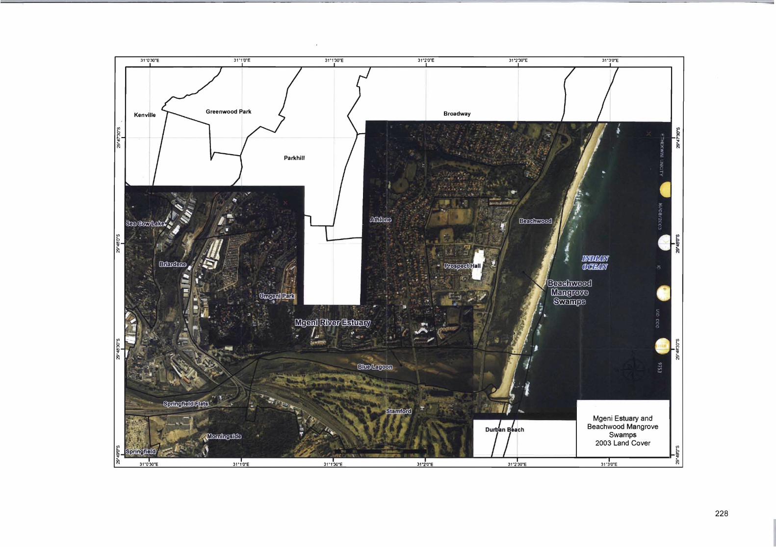
31
Parkhill
Mgeni Estuary and Beachwood Mangrove
Swamps 2003 Land Cover
228
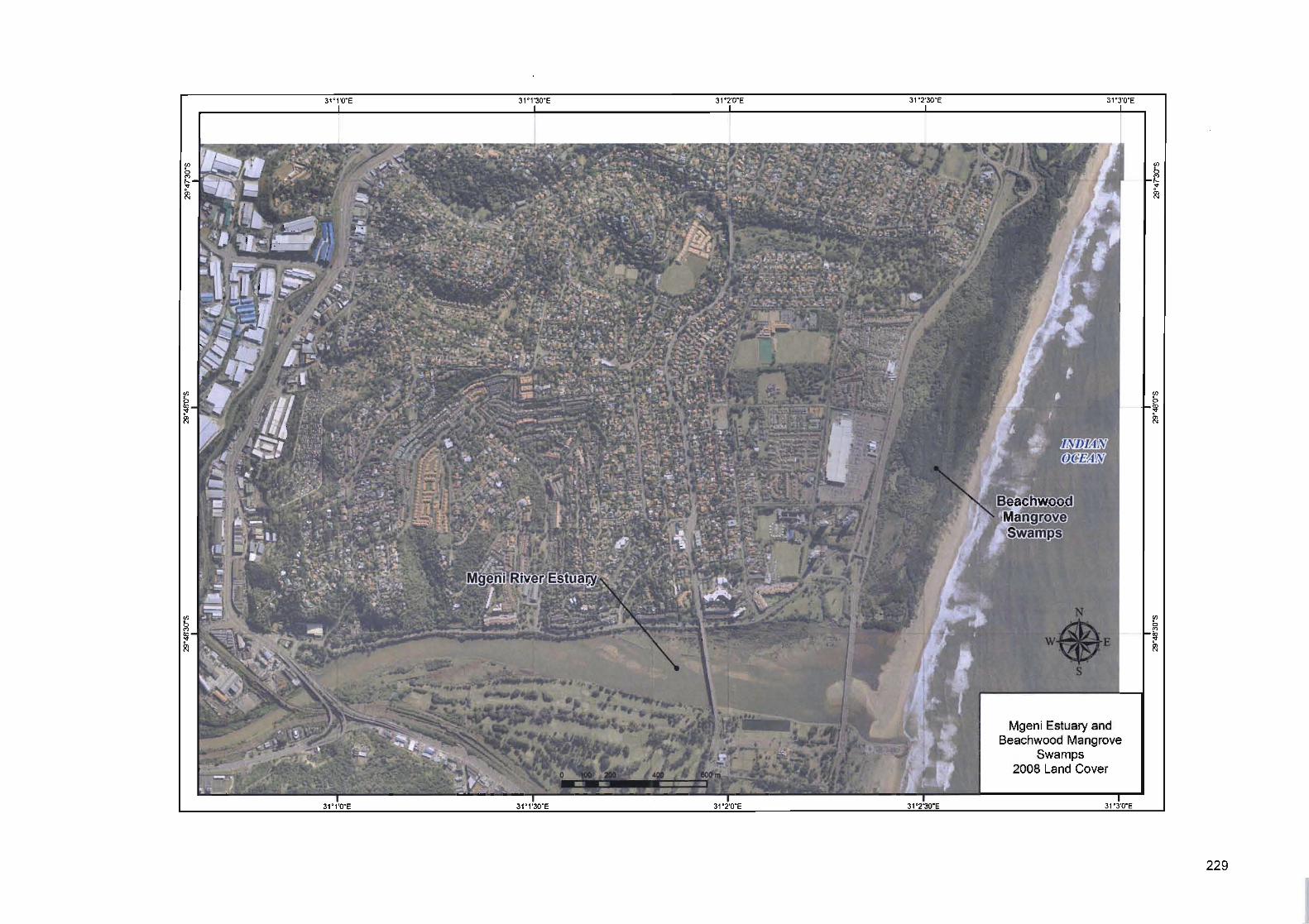
31
Mgeni Estuary and Beachwood Mangrove
Swamps 2008 Land Cover
229