The Value of a Statistical Life in aDictatorship: Evidence from Stalin∗

Paul Castaneda Dower

University of Wisconsin-Madison

Andrei Markevich

New Economic School

Shlomo Weber

New Economic School

February 26, 2019

Abstract

We examine the value of a statistical life (VSL) in interwar Soviet Union.Our approach requires to address the preferences of Stalin. We model theseon the basis of the policy of statistical repression, which was an integral partof the Great Terror. We use regional variation in the victims generated bythis policy to structurally estimate the value that Stalin would have beenwilling to accept for a reduction in citizens’ fatality risk. Our estimate ofthis value is about 43,000 USD, roughly 6% of the VSL estimate in 1940’s USand 29% of the VSL estimate in modern India.

JEL Codes: J17; I30; N44; P51.Keywords: Value of a Statistical Life; Autocracy; Dictatorship; Stalin; GreatTerror.

∗Contact information for authors: Castaneda Dower, pdower@wisc.edu; Markevich,amarkevich@nes.ru; Weber, sweber@nes.ru. We thank Steven Durlauf, Don Filtzer, Paul Gre-gory, Mark Harrison, James Heinzen, Natalya Naumenko, Laura Schechter and Ekaterina Zhu-ravskaya for their comments. The authors wish to acknowledge the support of the Ministry ofEducation and Science of the Russian Federation, grant No. 14.U04.31.0002. Markevich wouldlike to thank the Hoover Institution. We would like to thank Ivan Susin for research assistance

2

1. Introduction

Any complex society confronts a trade-off between economic gain and citi-

zens’ fatality risk. To assist in the analysis of this trade-off, Schelling (1968) and

Dreze (1962) introduced the concept of the value of a statistical life (VSL), which

amounts to the value of the societal sacrifice for an incremental reduction in a

fatality or hazard risk (Viscusi and Aldy 2010; Ashenfelter 2006). Despite es-

timating VSL in different political contexts, e.g. Ashenfelter and Greenstone

(2004) in the US, Kim and Fishback (1999) in South Korea and Leon and Miguel

(2017) in Sierra Leone, the literature has exclusively used this framework to elicit

citizens’ preferences.1 However, how much, if at all, citizens’ preferences impact

policy-making depends upon a country’s political institutions and how politi-

cally empowered citizens are. Indeed, in some political regimes, the elite’s pref-

erences could be more significant for determining policy choices than those of

citizens (Acemoglu and Robinson 2012).

In order to highlight the difference in decision-making on fatality risks be-

tween policymakers and citizens, we estimate the monetary value placed by a

dictator on the statistical life of his subjects. In a dictatorship, the entitlement

to the preferred state of the world belongs to the dictator and his preferences

determine policy choices. Since VSL is commonly defined as citizens’ willing-

ness to pay for a risk reduction, we, therefore, define the dictator’s valuation in

terms of willingness to accept (WTA) compensation for a reduction in citizens’

fatality risk. That is, we envision a hypothetical bargaining process (with an

imbalance in bargaining power) between the citizens and the dictator over cit-

1The only exception that we have uncovered is Rohlfs et al. (2016), who estimate the im-plied value of statistical life based on military decisions during WWII, but they assume that themilitary maximizes social welfare and equates marginal cost with marginal benefit.

3

izens’ fatality risk.2 Since policymakers and citizens may have conflicting pref-

erences over certain types of risks, the policymakers’ WTA and citizens’ WTP

could differ substantially. To make a potential gap in preferences most vivid,

we examine policy-making in Joseph Stalin’s dictatorship for a brutal policy of

the Great Terror in 1937 - 1938 aimed at the elimination of a potential fifth col-

umn and increasing his chances of preserving political power in case of a war

(Khlevnuk 2009, Harrison 2008).3

The Great Terror had a substantial random component that raised the fatal-

ity risk of Soviet citizens. The screening technologies of enemy identification

of Stalin’s secret police were far from perfect (Gregory et. al. 2011) and, in fact,

the bulk of victims were statistical in nature (Gregory 2009).4 The total range of

Great Terror affected about 1,500,000 Soviet citizens, 700,000 of which were exe-

cuted (Gregory 2009). We must point out, though, that statistical repression was

not an exclusive feature of dictatorial regimes.5 Democracies also have imple-

mented statistical repression when facing regime insecurity as it has been done

by Franklin D. Roosevelt who ordered the forced relocation and incarceration

2We could have used an alternative concept, the dictator’s willingness to pay for a reductionin the fatality risk of citizens, inserting dictator in place of citizen. No matter how this valuationis defined, we stress that it is conceptually distinct from the standard concept of VSL. One cansee this clearly through Thomas Schelling’s cleverly titled, “The life you save may be your own.”The VSL is derived from a citizen expressing this value in terms of a risk that the citizen faces.It is a measure of subjective valuation of own life. In contrast, the dictator’s valuation is notsuch a construct. The dictator’s valuation need not be the subjective valuation of own-life fa-tality risk since the risk may or may not be one that the dictator faces. Modeling this valuationas a bargaining process respects this distinction while still grounding the concept in the VSLliterature.

3Fifth column refers to a group within a society that works to undermine the society fromwithin. The term became popular after the Spanish Civil war, when the nationalist generalEmilio Mola told in an interview in 1936 that four columns of his army would attack Madrid, andthe fifth column of his supporters inside the city would undermine the republican governmentfrom within.

4We distinguish between statistical and identified victims. The former are victims who wereselected by a probability law whereas the latter were evidentially identified.

5Statistical repression refers to actions that physically suppress individuals of societythrough statistical discrimination.

4

of over 60,000 US citizens of Japanese ancestry, targeted purely on the basis of

population shares in a given location.

In order to isolate the component of statistical terror, we focus on the “na-

tional operations” of the Great Terror, providing a clear population target in

which ethnicity alone determined a policy-driven increase in fatality risk. Due

to population sizes and data availability, we restrict attention to the operations

against ethnic Poles and Germans, whom the government considered as poten-

tial traitors in war time. More than 195,000 Soviet citizens were arrested, with

two-thirds of these having been executed, under “national campaigns” against

Poles and Germans in 1937 - 1938 (Petrov and Roginskii 1997; Okhotin and Ro-

ginskii 1999). On average, the fatality risk imposed by this policy of statistical

terror was around twenty times higher than the contemporary US traffic fatal-

ity rate.6

The scope of the repressions had substantial regional variation in the dis-

tribution of terror victims and, in particular, there were a larger number of vic-

tims in the border areas. This was in line with the prevention of Stalin’s feared

scenario of a potential alliance between internal and external enemies, which

posed a stronger threat in border regions (Harrison 2008). We assume that

Stalin’s objective in implementing the Great Terror was to enhance the chances

of the survival of his regime in each region of the country, subject to the direct

economic loss of human life. Therefore, we derive Stalin’s decisions from the

presumed balance between the loss of economic output and enhancement of

regime survival. In this way, we can uncover Stalin’s WTA for a reduction in fa-

tality risk equivalent to the gain of one Soviet citizen’s statistical life, which we

6This incremental risk is larger than what is typically studied in the VSL literature, e.g. Ashen-felter and Greenstone (2004).

5

call the value of statistical life in the dictatorship (VSLD).

A priori, we do not know the value placed by Stalin or whether VSLD dif-

fered dramatically from Soviet citizens’ willingness to pay for a reduction in

fatality risk. A glance at the raw numbers, however, suggests that the brutal-

ity of Stalin’s regime was not without historical comparisons, and the intensity

of statistical terror appears to not have reached the most egregious instances

of these arbitrary mass killings by other dictators of the modern world. Dicta-

tors from Mao Zedong in China to Macias Nguema of Equatorial Guinea have

implemented policies of arbitrary and statistical mass killings of similar magni-

tude in terms of population shares as Stalin did in order to further improve their

regime’s survival.7 Idi Amin Dada of Uganda killed an estimated 100,000, many

of which were arbitrary killings of civilians, out of a population of 11 million,

roughly double the rate of the Great Terror overall.8 Since the world’s dictators

likely have heterogeneous preferences, estimates of VSLD should vary and, in

principle, one could replicate our method for other dictators, enabling a VSLD

ranking of dictators.

Using a newly constructed data set on the regional distribution of victims of

Stalin’s “national operations” against Soviet Poles and Germans in 1937-38, we

structurally estimate the parameters to recover Stalin’s preferences. This allows

us to specify the indifference curve that imbeds Stalin’s revealed-preferred pol-

icy choice. We use the slope of this curve at meaningful points to determine

Stalin’s VSLD. We find that Stalin would have been willing to accept a little more

than $43, 000 US 1990 for the reduction in citizens’ fatality risk equivalent to

7Our comparisons purposefully exclude cases of overt genocide as well as targeted suppres-sion of militarized anti-state groups.

8See Mass Atrocity Endings at https://sites.tufts.edu/atrocityendings/ . For this particularcase, the website cites the International Commission of Jurists (1977).

6

one statistical life. This magnitude is stable across a wide variety of robustness

checks. While this value is sizeable, it is far below what it could have been had

Stalin cared more for the survival of his regime or would stop at nothing to en-

sure its survival. At the same time, the value is far from what it would be had he

not been willing to put his citizens lives at risk to improve the likelihood of his

regime’s survival.

Comparing Stalin’s valuation with the value of a statistical life under democ-

racies (and assuming that Soviet citizens had similar preferences, on average,

as other countries at similar levels of development), we notice substantial wel-

fare gains from curtailing the policy of statistical terror. The magnitude of these

welfare gains contributes to our understanding of economic development in

non-democracies. If dictators systematically impose higher risks of fatality on

its citizens than would have otherwise been imposed had citizens been em-

powered, then this policy distortion could explain the difference in outcomes

in these regimes and the policy decisions and economic processes that gener-

ate them, such as the accumulation of human capital or the allocation of in-

vestments. Obviously, with only one observation of VSLD, we cannot establish

i) whether the difference between VSLD and VSL is related to the risk environ-

ment of citizens and ii) that democracies have less of a difference, on average,

between VSLD and VSL for a given set of policies. Thus, an important research

agenda that our analysis makes possible would be to investigate whether both

of these hypotheses hold.

Our analysis contributes to the debate on the nature of the Great Terror and

Stalin’s repressions. Historians have suggested a broad set of explanations of the

phenomena: from an innocent dictator (Barnett 2006) to a dictator merely re-

7

sponding to the demand for terror from below (Getty and Naumov 1999; Gold-

man 2007). In route to obtaining our estimate of the value of a statistical life, we

develop a view, which portrays Stalin as a strategic decision-maker, who relied

on coercion to achieve his economic and political goals, taking into account

the costs of his policies (Ilic 2006; Harrison 2008; Gregory 2009; Khlevnuk 2009;

Harris 2013).

Estimating the value of a statistical life in dictatorships also has profound

policy relevance. With such an estimate, countries can better influence and un-

derstand how dictators will respond to internationally imposed policies such

as economic sanctions to discipline a political regime, provided that the dic-

tators behave strategically and economic values enter their objective function.

Dictators, just as with their democratic counterparts, can improve the design

of domestic policies by using VSL and VSLD estimates. In Stalin’s case, and

specifically for the broader policies of the Great Terror, more effective and cred-

ible communication of Stalin’s preferences to his subordinates may have bet-

ter solved the principal-agent problems that were profoundly at work in other

aspects of the Great Terror (Gregory 2009). There are no doubt other domes-

tic and international policy decisions (transportation, environmental regula-

tions, medical interventions) that would be assisted by the analysis of the value

of statistical life of both citizens and policymakers under alternative political

regimes. For example, Miller (2000) suggests that VSL could inform how Kuwait

should have been compensated for the Gulf War.

The rest of the paper proceeds as follows. In section 2, we review the method-

ology of the value of a statistical life and discuss our approach for measuring the

value of a statistical life under dictatorships. Section 3 discusses the historical

8

details of the Great Terror and introduces our data. In section 4, we formalize

the trade-off between monetary gain and risk of fatality faced by Stalin in the

maximization of his objective function. Section 5 is devoted to the estimation

strategy. In section 6, we present the results and compare them with back-of-

envelope estimates of VSL according to the preferences of Soviet citizens and

state actors as well as estimates in the literature of the value of a statistical life

in democratic countries. Section 7 presents the sensitivity analysis, including

various robustness checks and a discussion of potential biases. Section 8 con-

cludes.

2. Fatality Risk in a Dictatorship

We start with the standard definition of the value of a statistical life, which is ex-

pressed in monetary terms and calculated on the basis of a small reduction in a

specified citizens’ fatality risk, spread across a large, clearly defined population

cluster.

Economists use both revealed and stated preference methods to estimate

citizens’ willingness to pay for a reduction in fatality risk.9 Since we can’t employ

stated preference methods for a historical episode, we instead rely on reveled

preference methods.

Several authors have suggested that citizens’ WTP may change under alter-

native institutional arrangements (Kim and Fishback 1999; Ashenfelter 2006).

Building on this logic, we argue that, in addition to citizen preferences, institu-

tional differences with regard to the entitlement of the decision on the level of

9See Viscusi (2003) for an overview of these methods.

9

fatality risk that policy targets could impact VSL estimations.10 Whoever pos-

sesses the entitlement determines whether willingness to pay or willingness to

accept is the object of interest. If one assigns the entitlement to citizens, then

we should estimate citizens’ willingness to accept for an increase in fatality risk

and, by extension, policymakers’ willingness to pay for an increase in fatality

risk. Typically, however, economists estimate citizens’ willingness to pay for a

reduction in fatality risk, implying the entitlement belongs to the policymak-

ers, who must therefore compare this willingness to pay to their willingness to

accept for a reduction in citizens’ fatality risk.

In democratic settings, where citizens ultimately bear the cost of risk reduc-

tion policies through taxation, citizens defer their entitlement to risk reduction

to their representatives on the basis of a social contract. A risk-reduction pol-

icy is usually adopted if it enhances social welfare. In effect, the policymakers’

preferences are disciplined by citizens’ preferences.

In contrast, in dictatorships with limited political representation for citizens,

the entitlement over the preferred state of the world belongs to the dictator. If

policy-making is driven by the dictator’s preferences, any specified risk used to

estimate VSL must be viewed in terms of the dictator’s objective, which may dif-

fer or even contradict the citizens’ objectives. There is no institutional guaran-

tee that the dictator would base policies on any given set of agents’ preferences

(although he/she may certainly do so). Hence, to analyze a proposed policy of

citizens’ fatality risk reduction, the dictator’s willingness to accept for a reduc-

tion in citizen’s fatality risk, rather than citizens’ WTP is the primary object of

10This point is not exactly new and has roots in an old debate on the role of economists inpolicy-making (Banzhaf 2009). The losers of the debate argued that policymakers had multi-ple objectives besides economic efficiency and economists should incorporate these objectivesdirectly in the normative analysis of policies.

10

interest. To head off any confusion due to terminology, we point out that, in

terms of willingness to pay, the dictator’s VSL would be given in terms of an in-

crease in fatality risk, more aptly called the value of a statistical death (i.e. in

the standard use of VSL for citizen preferences, the WTA counterpart of WTP

refers to an increase in fatality risk whereas for the WTP counterpart of WTA for

the dictator refers to an increase in fatality risk). We therefore define the dic-

tator’s VSL (VSLD) as the monetary value that the dictator would be willing to

accept for an incremental reduction in citizen risk of fatality, spread across a

large population, equivalent to preventing the loss of one life in expectation.

Importantly, citizens’ WTP for a reduction in fatality risk is still a useful con-

struct in a dictatorship. It just does not tell us all the information we would

like to know for policy-making. Investigating citizens’ WTP in a dictatorship

presents additional difficulties. Standard methods, such as contingent valua-

tion or using wage/occupational risk differentials, may have less desirable prop-

erties when estimating VSL in dictatorships. For example, if preference hetero-

geneity is purposefully suppressed, then it will be more difficult to credibly elicit

true preferences or, if decentralized decision-making is suppressed, it may be

difficult to recover preferences from price or cost data.

Consider the hedonic price regressions that economists often use to esti-

mate citizens’ willingness to pay for a risk reduction. Policymakers use the es-

timates of citizens’ preferences from these regressions by making an analogy

between the type of risk the policy would impact and the on-the-job risk that

workers face. Workers voluntarily choose one job with a certain level of fatality

risk and wage over another job with a different level of fatality risk and wage and

competitive markets accurately price opportunity cost of taking a different job.

11

In a democracy with well-developed labor markets, each of these assumptions

are reasonable. In a dictatorship, all three assumptions are problematic. Hence,

relying on the tangency condition to establish valuations based on unobserved

preferences is questionable. Instead, we model the dictator’s objective function

explicitly and can therefore fully specify indifference curves and report more

meaningful marginal valuations. Notice that we do not need to worry about the

usual selection issue involved in estimating WTP as the dictator’s problem ex-

actly reveals his willingness to accept for saving a statistical life. We do however

discuss several other potential sources of bias in section 7.

To illustrate these important differences, we introduce figures 1 and 2 for

the type of risk imposed on Soviet citizens during the Great Terror. Statistical

or random terror increased the likelihood that the regime would survive but

also increased the fatality risk of the citizens.Opportunity costs were the only

disciplining force that limited the dictator’s policy of statistical terror. Figure 1

represents this unfamiliar fatal trade-off for policy-making in a dictatorship and

figure 2 shows the same relationships in the familiar setting of policy-making in

a democracy. For both figures, the y-axis is wealth in monetary terms, the x-axis

represents citizens’ fatality risk, bounded between zero and one; the blue-line

represents the indifference curve of a representative citizen and the red-line

represents the indifference curve of the policy-maker.

In terms of the citizens, the two figures are the same. Citizens’ preferences

are upward sloping at an increasing rate, that is more and more wealth is re-

quired to make the citizen indifferent as the fatality risk increases. The preferred

point for citizens is at point A or zero fatality risk from statistical terror.

The two figures differ with respect to the policymaker. In figure 1, the dicta-

12

tor’s indifference curve is downward sloping due to the dictator’s desire to stay

in power. The only institutional discipline the dictator faces is the opportu-

nity cost of the loss of citizens’ lives, their contribution to the gross domestic

product, which in expectation is downward sloping at a constant rate. The dic-

tator prefers policy pointB, which is implemented despite the fact that citizens

would be willing to compensate the dictator for a reduction in fatality risk. Note

that, regardless of citizens’ WTP, in this example, there will be a positive level of

fatality risk due to the steepness of the dictator’s preferences as the fatality risk

declines. In figure 2, quite a different picture emerges due to the fact that the

policymaker has similar preferences to citizens, perhaps because of humanitar-

ian reasons or because they care about their constituents’ well-being by insti-

tutional design. The policymakers also prefer point A, even if they have flatter

preferences than the citizens have, since the budget constraint is downward

sloping, i.e. it actually costs wealth to increase fatality risk for a policy of statis-

tical terror.

3. Stalin’s Policy of the Great Terror in 1937-1938

The dominant rationalization of Stalin’s Great Terror policy, which cost at least

seven hundred thousand lives of Soviet citizens, refers to Stalin’s preparation

for a new great war and his concerns on the emergence of the “fifth column” in

the rear in the war time (Khlevnuk 2009, Harrison 2008). The capture of power

by the Bolsheviks following Russian defeat in the First World War taught a pro-

found lesson about the prospect for regime change in the aftermath of an un-

successful war. Stalin particularly feared the potential coalition between inter-

nal and external enemies and attempted to prevent its emergence even at high

13

costs. Stalin’s first deputy, Vyacheslav Molotov, in an interview in the 1970s,

twenty years after Stalin’s death, explicitly justified the Great Terror because

it weeded out potential traitors in the USSR so that the feared alliance of for-

eign and domestic enemies had not come to fruition during the Second World

War (Chuev 1991 P. 391).11 “National operations” against ethnic minorities of

neighboring mother-countries that posed a future war threat provides further

grounds for such an interpretation.

“National operations” were an important component of the Great Terror

policy.12 They produced more than a third of all victims (247,000 out of about

700,000). Ethnic Germans and Poles formed the two largest groups among vic-

tims of “national operations”. This was due to the relatively large size of these

minority groups and the threats posed to the USSR from Germany and Poland

in the late 1930s. Under Polish and German campaigns, 140,000 thousand and

55,000 Soviet citizens were arrested correspondingly. In addition to these two

major minorities, national operations affected Soviet Romanians, Greeks, Lat-

vians, Estonians, Lithuanians, Fins, Bulgarians, Iranians, Afghans, Koreans, Chi-

nese, and Japanese. Execution rates, i.e. a ratio of executions to all arrests,

were substantially higher for the “national operations” 73.66 percent on average

(79.44 percent for the victims of the campaign against Poles and 76.17 percent

for the German campaign) in contrast to the 43.3 percent execution rate dur-

ing the Great Terror years and 14.3 percent average execution rate under Stalin

(Petrov and Roginskii 1997; Okhotin and Roginskii 1999).13

11Archival documents demonstrate that Stalin himself believed that betrayals were the dom-inant reason of defeat of the Republicans in the Spanish Civil War happening at the same time.The Great Terror in the USSR went in parallel with attempts of the Spanish communists (di-rected from Moscow) to eliminate traitors among the Republicans in Spain (Khlevnuk 2009).

12See Appendix A for further historical details about the Great Terror.13Those victims who were spared execution were sent into labor camps (the Gulag) where life

and working conditions were tough. The mortality rate in the Gulag was between four and six

14

One could view the share of targeted ethical minorities in a region as a proxy

for the level of the local internal threat observed by the dictator. Using the pop-

ulation census, we have access to the same information on potential disloyalty

that the dictator had. This makes the “national operations” component of the

Great Terror particularly attractive for the study of the dictator’s preferences. We

limit our analysis to the largest two minorities, Germans and Poles, because of

data availability.

During “national operations”, Soviet citizens of targeted ethnicities, and es-

pecially those with special ties to their “mother countries” were under a higher

risk of arrest and being labeled spies. Particular ethnic groups whose loyalty

was especially problematic in the eyes of the dictator were in danger first of all;

e.g. in the case of Soviet Poles the secret police paid special attention to former

prisoners of Soviet-Polish war, who remained in the USSR, to former Polish cit-

izens, who fled into the USSR during the 1920s and 1930s, to former members

of Polish social party, to leaders of Polish national movement in the districts

with substantial Polish minority etc. In practice, implementation and screen-

ing technologies for true enemies were poor. Many loyal Soviet citizens became

victims as a result of the statistical nature of the Great Terror. The Soviet gov-

ernment was well aware about that. Stalin believed that if at least five percent

of suspects were correctly identified as true enemies that would be qualified as

a success (Stalin’s speech at the meeting of the High Military Council on June

2, 1937, cited in Khlevnuk 2010 Pp. 300-1). In other words, the Great Terror,

including its “national campaigns” component, implied additional fatality risks

to Soviet citizens.

times higher than the mortality rate of the corresponding ”free” population (Vishnevskij 2006p. 434). The Gulag composed about two percent of the Soviet labor force and produced aboutthe same share of GDP (Lazarev and Gregory 2003).

15

The Soviet archives clearly show that Stalin himself made the key decisions

about the Great Terror (Gregory 2009, Khlevnuk 2010), and the terror policy,

therefore, represented the dictator’s preferences. Stalin initiated the policy in

1937 and terminated the campaign in late 1938. In particular, the center closely

monitored the implementation of the “national operations” using the so called

“album procedure”. In each region, lists of arrested citizens and implied sen-

tences were recorded in special albums, which had to be sent to Moscow for a

final approval by the commission consisting of the All-Union Minister of Secret

Police and the All-Union Public Prosecutor (Petrov and Roginskii 1997; Okhotin

and Roginskii 1999).

The government planned and implemented mass repressions as a top se-

cret operation. There was no mention of them either in official media or in the

public sphere. The secret police had to search for, identify and punish poten-

tial enemies without any publicity. For that, the government heavily simplified

the judicial procedure during the “national operations”. Once the secret police

arrested a victim, it had to produce a short profile of the victim and to suggest a

sentence. Next, on the basis of these documents, a regional ”dvojka”, i.e. a com-

mission consisting of two officials (dvojka) - a head of regional secret police and

a regional public prosecutor, had to make a decision on the sentence, choosing

between an execution and imprisonment in Soviet labor camps for 5 or 10 years.

Decisions were taken in absence of the accused citizen and without the right to

appeal. The only supervision was from Moscow officials who followed the im-

plementation of ”national operations” and had to make the final approval of ar-

rests (via “album procedure”). The center weakened its control with an increase

of scope of repressions. When a rising number of arrested citizens caused sub-

16

stantial delays in Moscow approvals in September 1938, i.e. two months before

the termination of the Great Terror policy in November 1938, Stalin simplified

the procedure further. Local secret police offices got more power in the repres-

sion decision 14. Accordingly, regional variation in repressions during the last

two months of the Great Terror might to a lesser extent reflect the original pref-

erences of the dictator because of initiatives from below and the differences in

repression capacities of local administrations of the secret police.15

We construct a novel dataset on regional variation in implementation of the

Great Terror in 1937-1938, combining recent works by historians (Petrov and

Roginskii 1997; Okhotin and Roginskii 1999) and the 1939 Population Census

(Polyakov 1992).16 Table 1 presents summary statistics of available data. There

were about 2,700,000 people in an average Soviet region. Among them, there

was a bit less than 2,000,000 that lived in the countryside and about 950,000

were illiterate, capturing the levels of urbanization and human capital in a re-

gion. The average region consumed 641 million kilowatt hours of electricity,

which measures local economic development.17 During the Great Terror years,

in an average region, about 25,000 people were arrested because of political

reasons, or about 0.9 percent of total population. About 1,000 of them were ar-

rested as a part of the operation against Germans and about 2,200 as a part of

the operation against Poles. Out of these arrests, about 750 Germans and 1,850

Poles were executed in an average region. The rest were sent to the Gulag. Both

14Special commissions of three persons (trojka), which in addition to dvojka members in-cluded regional party leader, were established in each region. They temporally got the right ofthe final approval of repression decisions instead of Moscow.

15E.g. during the last phase of “national operations”, the share of titular nationals amongvictims was only about two-thirds (Petrov and Roginskii 1997; Okhotin and Roginskii 1999).

16A detailed history of Stalin’s repressions is still a work in progress (Unge, Bordukov and Bin-ner 2008). Many aspects of this policy remain unknown. In particular, the spatial distributionof victims of “national operations” is known only for Germans and Poles.

17Electricity output is from Naumenko (2019).

17

the number of arrests and executions of Poles and Germans varied substantially

across regions.

On top of human losses, the policy of Great Terror was costly in other re-

spects. First, operational costs of the terror campaign were 75 million rubles

in 1937 and another 100 million in 1938, i.e. about 0.05 percent of 1937 GDP

(Mozokhin 2011 pp.189-200)18. Second, the Great Terror was accompanied by

economic difficulties and slowdown of the economy of the USSR (Davies 2006).

4. A Model of Dictator’s Fatal Trade-off

Consider a country consisting of J regions, that includes both border and inte-

rior regions.19 The population of the region j in J is denoted by Nj . The total

population of the country is

N =J∑j=1

Nj.

The country is ruled by a dictator,D, who is driven by two factors: the coun-

try’s domestic product and the likelihood of his survival under an internal threat

posed by the presence of the potential enemies.20 Thus, the dictator’s objective

function is denoted by D(Y, S), where Y is output, and S is the likelihood of

regime’s survival in face of the threat posed by the possibility of a coalition be-

tween internal and foreign enemies. Obviously, the value of the objective func-

tion is increasing in both variables, the output and the probability of survival.

18The Secret Police asked for another 70 million to cover 1938 operation costs, but the resultof this request is unknown (Mozokhin 2011 p. 200).

19The distinction between these two types of regions will be made later.20We do not model the threat from actual enemies who are identifiable by the dictator. The

dictator’s secret police could identify and arrest enemies in both interior and border regions, butthese identifiable enemies are not statistical in nature. For simplicity, we assume that screeningabilities of the secret police are the same in each region, and do not model identifiable victimsexplicitly.

18

In order to balance a challenging model (no a priori knowledge of dictator’ pref-

erences towards risk) with its empirical tractability, we make a restrictive mod-

eling choice and choose the widely-used Cobb-Douglas functional form:

D(Y, S) = Y αS1−α,

where α is the parameter between 0 and 1, which indicates the dictator’s view of

tradeoff between the national product and the probability of staying in power.

If α is close to zero, then the dictator is mostly preoccupied with his own sur-

vival while almost disregarding the value of total production. If, conversely, α

is close to one, the dictator is focused on the production side without being the

preoccupied with the survival threats.21

To comment of our choice of specification, we must mention that we follow

the literature on the topic (e.g, Aldy and Viscusi 2007), where the VSL is usually

considered as the marginal rate of substitution between wealth and the prob-

ability of survival. However, the difference between our specification and the

standard approach, where the value of α is determined by the survival probabil-

ity, lies in the fact that the derivation of the VSL depends on individuals’s ability

to perceive and estimate the value of risk reductions. The issue is complicated

as it is, but more so in our setting when we have only an indirect knowledge

of the dictator’s preferences. Thus, we opted for a fixed value wealth-survival

probability trade-off. It is obviously a tractable FOC and offers us a clear em-

pirical path for our estimation purposes. Moreover, the importance of regional

integrity suggests that we lose little when abstracting from scale effects and,

since empirically we don’t know the distribution of output/probability of sur-

21The choice of a CES functional form would require estimating an additional parameter andfurther complicate the analysis without a clear justification for doing so.

19

vival within regions, we must in any case represent preferences in terms of the

regional aggregates.

To enhance the value of his objective function, the dictator may implement a

policy tool of the elimination of potential internal enemies. We assume that the

population of each region j is divided in two groups, loyal citizens and potential

enemies, where the number of the latter is denoted by Mj .The dictator chooses

τj ∈ [0,Mj], which corresponds to the target level of his elimination policy in

region j. It would be useful to point out that the group of potential enemies, in

our case ethnic minorities, faces a risk of fatality which is stochastically related

to the dictator’s policy. This level is achieved by imposing a fatality risk of τjMj

on

each of the Mj potential internal enemies in the region.

Let us examine the impact of such a policy both on production and the sur-

vival probability. Our analysis will address the dictator’s policy in all regions

separately.

Production

We assume that the output Yj is produced by the means of a unit linear pro-

duction function that utilizes the labor supply in each region.

Yj ≡ Lj.

Before the realization of the statistical terror policy, the population of each

region determines the supply of labour

L0j = Nj.

20

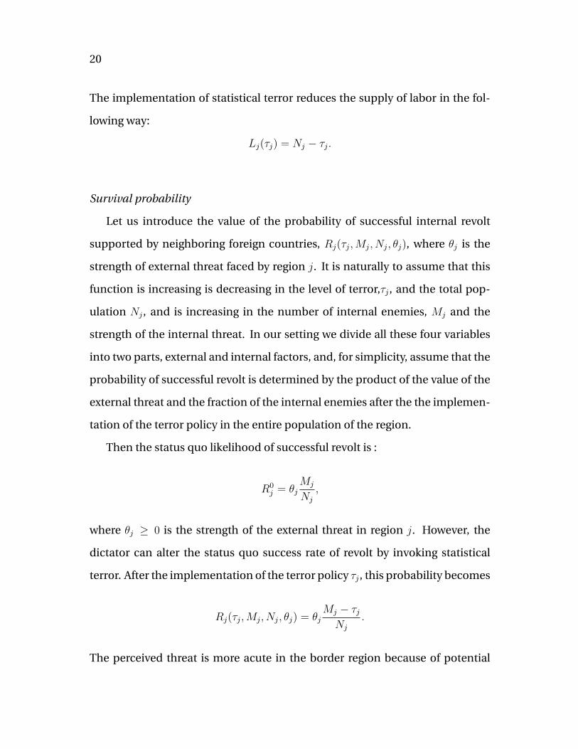
The implementation of statistical terror reduces the supply of labor in the fol-

lowing way:

Lj(τj) = Nj − τj.

Survival probability

Let us introduce the value of the probability of successful internal revolt

supported by neighboring foreign countries, Rj(τj,Mj, Nj, θj), where θj is the

strength of external threat faced by region j. It is naturally to assume that this

function is increasing is decreasing in the level of terror,τj , and the total pop-

ulation Nj , and is increasing in the number of internal enemies, Mj and the

strength of the internal threat. In our setting we divide all these four variables

into two parts, external and internal factors, and, for simplicity, assume that the

probability of successful revolt is determined by the product of the value of the

external threat and the fraction of the internal enemies after the the implemen-

tation of the terror policy in the entire population of the region.

Then the status quo likelihood of successful revolt is :

R0j = θj

Mj

Nj

,

where θj ≥ 0 is the strength of the external threat in region j. However, the

dictator can alter the status quo success rate of revolt by invoking statistical

terror. After the implementation of the terror policy τj , this probability becomes

Rj(τj,Mj, Nj, θj) = θjMj − τjNj

.

The perceived threat is more acute in the border region because of potential

21

coalition between neighboring foreign countries and internal enemies. To take

into account this observation, we set the value of θj to be the same and equal

to θ > 0 for all border regions, and to zero for all interior regions.22 Thus, the

probability of revolt in internal regions becomes zero, whereas in the border

regions it turns into

Rj(τj,Mj, Nj, θj) = θMj − τjNj

.

Note that the status quo probability of survival is given by

S0j = 1− θj

Mj

Nj

.

After invoking the terror policy τj , this expression becomes:

Sj(τj,Mj, Nj, θj) = 1− θMj − τjNj

.

for border region, while being equal to one for interior ones. That is, for interior

regions, the survival is guaranteed. Note that for border regions the value of Sj

under the total terror (τj = Mj) is also equal to one. The value of Sj in absence

of terror (τj = 0) is strictly greater than zero.

Let us now turn to the examination of the dictator’s objective function.

Objective function

In absence of statistical terror policy, expected dictator’s utility in a region j

is

D0j = (L0

j)α(1−R0

j )1−α.

22The main point here is to distinguish between interior and border regions. The specificassumption on the values of θj can be easily weakened.

22

Then, we derive the level of the objective function of Dj(τj,Mj, Nj, θj) in region

j:

Dj(τj,Mj, Nj, θj) = (Nj − τj)α(1− θj

Mj − τjNj

)1−α

.

First note that for interior regions τj = 0 and there is no terror policy.

For border regions, after taking logarithms, we obtain the first order condi-

tions with respect to τ in the following form:

− α

Nj − τj+

(1− α)θNj − θMj + θτj

= 0. (1)

Rearranging terms yields:

τ ∗j =(1− α)θ − α

θNj + αMj = (1− 1 + θ

θα)Nj + αMj. (2)

Let us make two observations:

The optimally chosen τ ∗j is decreasing in α. This relationship is intuitive.

As α increases, stability contributes less to the dictator’s objective function thus

reducing his optimal terror level. To show that take derivatives of (2) to get∂τ∗j∂α

=

−Njθ− (Nj −Mj). Since θ > 0 and Nj ≥Mj for any region, the whole expression

is always negative.

The optimally chosen τ ∗j is increasing in θ. This result illustrates the per-

nicious incentives of the dictator. An increase in the strength of the external

threat increases the incentives to engage in statistical terror. Simple algebra

shows that∂τ∗j∂θ

=αNjθ2

> 0.

23

5. Estimating VSLD

In this section, we describe how we obtain VSLD, using a revealed preference

approach. The first step is to recover the dictator’s preferences implied by the

model and the data. Then, once we have estimates of these structural parame-

ters, we calculate the marginal rate of substitution (MRS) between wealth and

regime survival. Finally, we compute the VSLD by converting this value to the

relevant units.

5.1. Estimation of the structural parameters

We assume a data generating process that results in the observable number of

victims of the national campaigns in a region, Kj , being a random variable that

depends upon, but is not fully determined by, the level of statistical terror cho-

sen by the dictator. Empirically, it would be difficult to claim that Kj = τj . In-

stead, Kj may capture identifiable victims, those who the secret police would

have implicated as committing crimes independent of the statistical terror, and

idiosyncratic deviations from the optimal level of statistical terror. We thus rep-

resent the observed number of victims in a region as:

Kj = τj + νj + εj

where τj is defined above as the optimal number of victims due to statistical

terror, νj captures the number of non-statistical, identifiable victims and εj rep-

resents the deviation from the optimum due to unknown factors.

Since all of the above components are unobservable to the econometrician,

we need to make several assumptions. For τ , we assume it is determined opti-

24

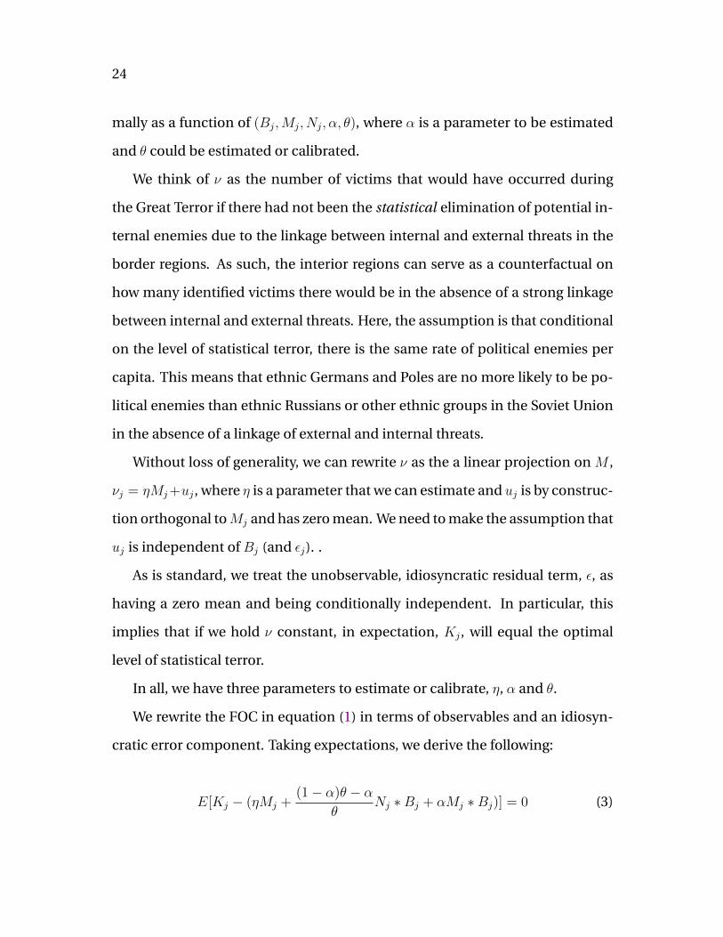
mally as a function of (Bj,Mj, Nj, α, θ), where α is a parameter to be estimated

and θ could be estimated or calibrated.

We think of ν as the number of victims that would have occurred during

the Great Terror if there had not been the statistical elimination of potential in-

ternal enemies due to the linkage between internal and external threats in the

border regions. As such, the interior regions can serve as a counterfactual on

how many identified victims there would be in the absence of a strong linkage

between internal and external threats. Here, the assumption is that conditional

on the level of statistical terror, there is the same rate of political enemies per

capita. This means that ethnic Germans and Poles are no more likely to be po-

litical enemies than ethnic Russians or other ethnic groups in the Soviet Union

in the absence of a linkage of external and internal threats.

Without loss of generality, we can rewrite ν as the a linear projection on M ,

νj = ηMj+uj , where η is a parameter that we can estimate and uj is by construc-

tion orthogonal toMj and has zero mean. We need to make the assumption that

uj is independent of Bj (and εj). .

As is standard, we treat the unobservable, idiosyncratic residual term, ε, as

having a zero mean and being conditionally independent. In particular, this

implies that if we hold ν constant, in expectation, Kj , will equal the optimal

level of statistical terror.

In all, we have three parameters to estimate or calibrate, η, α and θ.

We rewrite the FOC in equation (1) in terms of observables and an idiosyn-

cratic error component. Taking expectations, we derive the following:

E[Kj − (ηMj +(1− α)θ − α

θNj ∗Bj + αMj ∗Bj)] = 0 (3)

25

We then put in per capita terms where k and m are the per capita counter-

parts of K and M :

E[kj − (ηmj +(1− α)θ − α

θBj + αBj ∗mj)] = 0 (4)

We estimate α using (generalized) method of moments and the FOC as a

moment restriction. In our main analysis, we employ this sole moment restric-

tion.

Given our identification assumption about border, we have in effect two mo-

ment conditions, one for border regions and one for non-border.

E[Kj − ηMj] = 0∀ j with Bj = 0

E[Kj − (ηMj +(1− α)θ − α

θNj + αMj)] = 0∀ j with Bj = 1

We first estimate η using the non-border regions. Then, we estimate the mo-

ment given by the FOC for border and nonborder regions, plugging in our esti-

mate of η. To estimate both α and θ, our preferred estimation strategy, we use

the FOC along with our exogenous variables as instruments. To be precise, we

interact each of the following variables, the border indicator, the number of for-

eigners per capita and their interaction, with the FOC to generate additional

moment restrictions and estimate using generalized method of moments. Fi-

nally, we plug in our estimates into the equation for the VSLD, which we de-

scribe below. We obtain confidence intervals for VSLD and other parameters by

bootstrapping the whole procedure, with stratified re-sampling for border and

non-border.

26

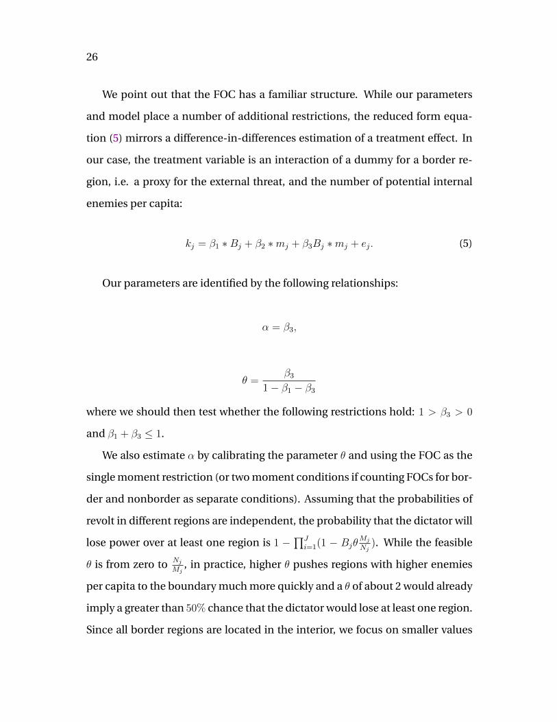
We point out that the FOC has a familiar structure. While our parameters

and model place a number of additional restrictions, the reduced form equa-

tion (5) mirrors a difference-in-differences estimation of a treatment effect. In

our case, the treatment variable is an interaction of a dummy for a border re-

gion, i.e. a proxy for the external threat, and the number of potential internal

enemies per capita:

kj = β1 ∗Bj + β2 ∗mj + β3Bj ∗mj + ej. (5)

Our parameters are identified by the following relationships:

α = β3,

θ =β3

1− β1 − β3

where we should then test whether the following restrictions hold: 1 > β3 > 0

and β1 + β3 ≤ 1.

We also estimate α by calibrating the parameter θ and using the FOC as the

single moment restriction (or two moment conditions if counting FOCs for bor-

der and nonborder as separate conditions). Assuming that the probabilities of

revolt in different regions are independent, the probability that the dictator will

lose power over at least one region is 1 −∏J

i=1(1 − BjθMj

Nj). While the feasible

θ is from zero to NjMj

, in practice, higher θ pushes regions with higher enemies

per capita to the boundary much more quickly and a θ of about 2 would already

imply a greater than 50% chance that the dictator would lose at least one region.

Since all border regions are located in the interior, we focus on smaller values

27

and explore higher values in the robustness section. We take two benchmark

cases: i) θ = .065, which corresponds to a 2.5% chance that the dictator would

lose at least one region and ii) θ = .125, which corresponds to a 5% chance that

the dictator would lose at least one region. We select these benchmarks in or-

der to follow the official Soviet military doctrine that stated that the Red Army

would defeat the enemy on foreign territory with an objective of no loss of So-

viet regions (Red Army Field Manual, 1939).

5.2. Estimating the VSLD

After estimatingα and using the objective function of the dictator, we can derive

the VSLD, which is a counterfactual value due to the nature of the dictatorship.

In the absence of market prices and voluntary action, the precise point of tan-

gency between the dictator’s budget constraint and his indifference curve has

limited meaning. In the border regions, for all α, MRS∗ =Njθ

at the optimum

due to the implied technological terms of trade, which are constant within each

region. This means that all α-types are observationally equivalent at this tan-

gency. Because of the endogeneity of citizen fatality risk in the dictator case,

we need structural assumptions (i.e. Stalin’s preferences) about how this risk is

determined to unpack the VSLD estimate.

Instead, we focus on the dictator’s WTA using the following thought experi-

ment. Holding the dictator’s utility constant at the optimum, we can ask what

value does the MRS take when the policy of statistical terror approaches zero

victims. This point is on the steepest part of the indifference curve within the

range of regime survival that the policy can affect. Thus, the slope at this point

yields the maximum value that the dictator would need to be compensated for

28

saving one statistical life.

As the first step, we obtain the indifference curve that intersects the opti-

mum. This utility level is u∗j ≡ L∗αj S∗1−αj , where L∗ and S∗ are the values of L and

S at the optimum. Holding the dictator’s utility level constant, for any L, S pair,

the marginal rate of substitution of output for regime survival is:

(1− α)α

L

S

While staying on the indifference curve that intersects the optimum, we

compute MRS at the point where S equals the baseline risk. This yields

MRS =1− αα

L∗j(S∗j )

1−αα (1− θMj

Nj

)−1α .

We plug in θ and α for θ and α, respectively.

Then, at the second step, we convert units of regime survival to units of cit-

izen fatality risk, since the obtained value of MRS is with respect to regime sur-

vival. That is, moving citizens’ fatality risk from zero to one does not move the

probability of survival of the regime in a border region from zero to one. Thus,

we need to multiply the MRS by (1 − (1 − θMj

Nj)) =

θMj

Nj, which is the length of

the interval as we move from a fatality risk for citizens of one to zero fatality

risk. Since M citizens facing a reduction in fatality risk of 1M

would produce a

gain of one statistical life, we divide by M . In this way, we get the value that one

would have to compensate the dictator for a reduction in fatality risk equivalent

to saving one statistical life.

Finally, we convert this value from units of output to units of monetary cost.

This final step consists of multiplying by g, the monetary value of per capita

29

output.

This procedure then results in:

V SLD ≡ g((1− α)(1 + θ(1− M

N))

1− θMN

)1α .

If the policymakers’ preferences perfectly reflect the median voter (pure democ-

racy), there would be no weight placed on regime survival, α = 1, and VSLD

would be equal to zero, technically, it would be less than or equal to zero. Recall

that, for this particular risk, the dictator and the citizen have opposing pref-

erences. A more democratic dictator, who valued regime survival less, would

be willing to accept a lower amount to reduce citizens’ fatality risk from statis-

tical terror, which is intuitive. As α moves away from one toward zero, VSLD

increases and does so quite rapidly as α approaches zero. If there were Coasean

bargaining between the dictator and the citizens or the broader international

community, one obvious result is that the more brutal the dictator is, repre-

sented as a lower α, the more compensation is needed to achieve a reduction in

citizen fatality risk.

6. Discussion of results

We start by presenting the results of the reduced-form regressions in Table 5. In

Column (1), we present the sparsest specification that still allows us to recover

the structural parameters of interest. The key effect of interest is the coeffi-

cient on the interaction term between Germans and Poles per capita and the

border region dummy. It is positive and statistically significant and it’s magni-

tude is large, implying an increase in the homicide rate represented in victims

30

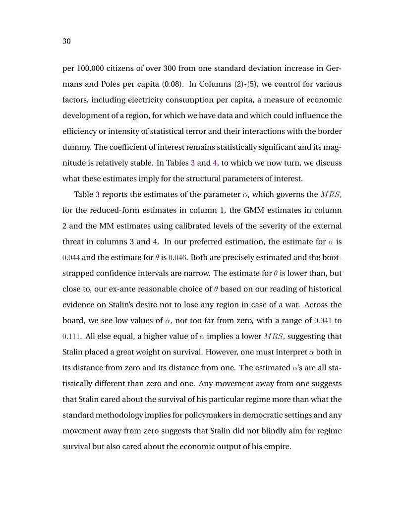
per 100,000 citizens of over 300 from one standard deviation increase in Ger-

mans and Poles per capita (0.08). In Columns (2)-(5), we control for various

factors, including electricity consumption per capita, a measure of economic

development of a region, for which we have data and which could influence the

efficiency or intensity of statistical terror and their interactions with the border

dummy. The coefficient of interest remains statistically significant and its mag-

nitude is relatively stable. In Tables 3 and 4, to which we now turn, we discuss

what these estimates imply for the structural parameters of interest.

Table 3 reports the estimates of the parameter α, which governs the MRS,

for the reduced-form estimates in column 1, the GMM estimates in column

2 and the MM estimates using calibrated levels of the severity of the external

threat in columns 3 and 4. In our preferred estimation, the estimate for α is

0.044 and the estimate for θ is 0.046. Both are precisely estimated and the boot-

strapped confidence intervals are narrow. The estimate for θ is lower than, but

close to, our ex-ante reasonable choice of θ based on our reading of historical

evidence on Stalin’s desire not to lose any region in case of a war. Across the

board, we see low values of α, not too far from zero, with a range of 0.041 to

0.111. All else equal, a higher value of α implies a lower MRS, suggesting that

Stalin placed a great weight on survival. However, one must interpret α both in

its distance from zero and its distance from one. The estimated α’s are all sta-

tistically different than zero and one. Any movement away from one suggests

that Stalin cared about the survival of his particular regime more than what the

standard methodology implies for policymakers in democratic settings and any

movement away from zero suggests that Stalin did not blindly aim for regime

survival but also cared about the economic output of his empire.

31

These estimates of α and θ translate into estimates of the VSLD and Table 4

reports the implied values. We report the average VSLD across the regions. To

get a sense of how precisely estimated this mean is, we report 95% confidence

intervals, which we obtain using bootstrapping methods. We find a value of

$43, 151 US 1990 in our preferred specification. In the estimations using a single

moment condition derived from the FOC and a calibrated θ, increasing θ does

not dramatically change the VSLD, mostly due to the fact that the estimate for

α must increase to fit the data and this offsets the increase in the VSLD due to

an increase in the external threat.

If we abstract from the actual policy outcome, we can explore how sensi-

tive VSLD is to changes in parameters. Figure 3 shows how the value of VSLD

changes for the average region if Stalin had had somewhat different prefer-

ences, holding θ fixed. We report these values for two different levels of θ, rep-

resenting alternative environments that Stalin may have faced. For θ values, we

chose the estimated level of θ according to our preferred estimation (0.046) and

the highest value of θ that we use when making calibrations (0.125). For conve-

nience, we have drawn a dotted vertical line at α = 0.044, representing Stalin’s

type in our preferred estimation. The points of intersection of this dotted line

and the curves give Stalin’s VSLD under these different strengths of the exter-

nal threat (for θ = 0.046, the intersection point gives our preferred estimate of

Stalin’s VSLD). For θ = 0.046, an α-type of 0.02 would result in a VSLD of ap-

proximately $160, 000, where as an α-type of 0.1 would result in a value of little

less than $24000, revealing that Stalin had an intermediate value, if our estimate

of θ is accurate. This intermediate value is deceptive, though, because moving

to the right on the x-axis, we can find dictators of “nearby” types, who would

32

not have initiated any positive level of repression when faced with the same re-

gional distribution of population groups. When θ = 0.125, VSLD is higher for

any given type, and increasingly so as α approaches zero. If this were the actual

level of θ in 1937-1938 in the USSR, a dictator of Stalin’s type (with alpha 0.044)

would have had a VSLD of roughly $226000 and, in such a case, we would have

observed, in expectation, all of the ethnic Germans and Poles being repressed

during the national campaigns.

What can we say about the value of Stalin’s VSLD? The first and most glaring

point is that this value is quite large compared to $ 0 US 1990 (or even nega-

tive values) that policymakers in a pure democracy would accept to reduce the

number of statistical victims in a policy of statistical terror. In a counterfac-

tual exercise, the average border region would have had to compensate Stalin

roughly about $300 million US 1990 to prevent the policy of statistical terror in

the region. Second, $43,151 is not terribly high, roughly equivalent to the net

present value of the per capita national income stream, if one had the prior that

Stalin would stop at nothing to maintain his grip on power.

In the model, Stalin would have been willing to accept this amount in ex-

change for one less statistical victim of terror. This is indeed an arresting re-

sult demonstrating the importance of institutions to discipline political deci-

sions when they deviate from citizens’ preferences. Even though Stalin behaved

strategically, and some would say rationally (see a discussion on that Barnet

(2006), Harrison (2006), Wheatcroft (2006)), his dictatorship as a political in-

stitution failed to prevent the implementation of policies that had dire effects

from both a humanitarian and a social welfare point of view.

Our estimates are also in line with an external estimate of how Stalin’s judges

33

valued the life of Soviet citizens. Heinzen (2016) provides archival examples of

revealed bribes which Soviet citizens paid to officials to escape punishment.

These historical anecdotes imply that one had to pay between 3000 and 40000

rubles to annul long prison sentences which might be viewed as the closest to

bribes for saving ones life. 23 To recalculate these figures in 1990 US dollars,

we use the exchange rate of 1.64 that yields a range between $4, 921 and $65, 616

US 1990 dollars.24 Of course, the use of bribes is problematic for a number of

reasons. First, we need to assume that the judges’ interests are based on a cal-

culation as to the value that Stalin places on the death of the citizen or pool

of potential offenders. This assumption seems reasonable as Stalin effectively

communicated his vision on repressions through the ranks (Gregory 2009). Sec-

ond, bribe payers are identified victims. However, if judges are willing to reveal

that sentences can be bought and each citizen had an ex-ante probability of

committing an offense while doing socially beneficial activities, then the possi-

bility of bribes would reduce citizen’s fatality risk. Finally, since we only observe

the bribes that citizens are willing or able to pay, we do not observe the full dis-

tribution of willingness to accept valuations.

In a more modern perspective, consider the cost of the Iraqi War aimed to

prevent future atrocities of the Hussein regime. In 1989, the GDP per capita of

Iraq was of a similar magnitude as the Soviet Union in the 1930s. If Saddam

Hussein had a similar VSLD as Stalin, then, for the total cost of the war (about

1.7 trillion 2011 US dollars, NATO/US could have paid the Iraqi dictator to re-

23Unfortunately, there are no examples of a judge took a bribe in a death penalty case in theknown archival documents. In private correspondence, Professor Heinzen argues that it “wouldhave been extremely risky, and likely would have subject the judge to the death penalty himself”.We thank Professor Heinzen for these details.

24To get the exchange rate, we divide Maddison’s estimate of Soviet GDP per capita in 1940in 1990 US dollars and Harrison’s estimate of Soviet GDP per capita in the same year in 1937roubles (Harrison 1996).

34

duce citizens’ fatality risk on the order of nearly 40 million statistical lives, 33%

more than the whole population of Iraq). Of course, this thought experiment

works better as a basis to understand the magnitude of the Stalin’s VSLD than as

a policy recommendation for handling future dictators, since there are strategic

issues and other costs involved in such an offer.

6.1. Comparison of results to estimates of VSL in democracies

How does Stalin’s VSLD compare to estimates of VSL in democracies? Before

answering this question, two disclaimers are in order.

First, the estimated VSLs from democracies are in terms of citizens’ willing-

ness to pay for a reduction in fatality risk, while the Stalin’s VSLD is in terms

of willingness to accept for a reduction in citizens’ fatality risk. It is important

to keep in mind that Stalin’s utility, based on the preferences that we impose,

is increasing in both wealth and citizen’s fatality risk. However, the compari-

son between citizens’ VSL and Stalin’s VSLD still has sense due to the fact that,

in a democracy, policymakers’ willingness to accept for a reduction in citizens’

fatality risk is disciplined by citizens’ willingness to pay. How disciplined the

policymakers’ WTA is provides the analyst how “democratic” the political insti-

tutions that can be measured across different types of de jure institutions are.

Second, we would like to underline that we are not comparing the value of

life under different political regimes. The value of life and the value of statisti-

cal life are conceptually distinct. In the colloquial sense, the value of life is, of

course, subjective and need not be measurable. As such, we do not consider

the value of life in an abstract sense and are certainly not suggesting that the

sanctity of life depends upon the political regime. In contrast, the value of a

35

statistical life is a meaningful comparison precisely because it could sensibly

vary by political regime, both in terms of policy-makers’ WTA and citizens’ WTP

as well as the types of fatality risks that policies affect.

Ashenfelter and Greenstone (2004) give a conservative estimate of 1.5 mil-

lion USD (1997) for modern US. This is roughly 50 times GDP per capita. Closer

to the time of Great Terror, Costa and Kahn (2004) provide a range for the VSL

estimate of 713,000 - 996,000 USD (1990) in the US in 1940. According to Maddi-

son daaset, the GDP per capita in the US was 7010 USD (1990) in 1940 or about

3.25 times higher than Soviet GDP per capita of 2156 USD (1990) in 1937. Per-

forming a benefits-transfer calculation using an income elasticity of 1.5 gives a

range for the VSL of $146,000 to $204,000 USD (1990).25

If we look to modern developing countries operating in a democratic mode,

Pakistan is probably the closest to Stalin’s Soviet Union in terms of GDP per

capita at $2240 USD (1990) in 2007.26 However, we choose to focus on India

with a GDP per capita of $ 2817 in 2007 because there are more VSL estimates

available and because India is also the hypothetical comparison group chosen

by Allen (2003) in his influential analysis of the comparative development of

the Soviet Union. For India, Bhattacharya et al. (2007) using a stated prefer-

ence analysis find a VSL of $150,000 USD (1990). Using wage differentials due

to occupational risk, Madheswaran (2007) finds $150,000-$300,000 USD (1990)

estimate of VSL.27

No matter how we approach the comparison group, the estimates of the VSL

in democracies are significantly higher in magnitude than the VSLD estimates

25We use 1.5 because Costa and Kahn find such an income elasticity. Leon and Miguel (2017)find 1.77 in modern day Sierra Leone. An elasticity of 1.7 would give a range of $129,000 to$180,000 USD (1990). An elasticity of 1 would give the range, $219,000-$306,000 USD (1990).

26Rafiq and Shah (2010) find an estimate of $122,047 to $313,411 of VSL in Pakistan.27Shanmugams (2001) finds a higher range of $760,000 to $1,020,600 USD (1990).

36

we find for Stalin’s dictatorship. Since dictatorships give less political empower-

ment to its citizens, we can not conclude that some type of Coasean bargaining

would have occurred between citizens’ representatives and the dictator in the

Soviet Union. But it seems reasonable to speculate that quite a few would be

willing to pay to avoid this fatality risk (and some did using bribes to judges as

discussed above).

One point that immediately follows from here is that in a democracy, even

if some policymaker were as brutal as Stalin and had VSLD>> 0, as long as

citizens were empowered with some political voice or control, no statistical ter-

ror would take place. More to the point, we can ask the following question:

how much weight would a democracy with a similar level of GDP per capita

have to place on Stalin’s preferences in order to implement a policy of statistical

terror with a positive level of expected victims? Taking our estimate of VSLD

and giving this valuation a weight of ω, along with the citizens’ valuation as

150, 000USD(1990), and giving citizens a weight of 1− ω, the ω′ that would yield

a positive level of victims would be ω′ ≥ 0.776 (ω′ = 150000/(150000 + 43180)).

This number assumes that the policy of statistical terror has no costs to im-

plement. Holding the dictator’s valuation constant, introducing costs would

raise the required ω. The important point from this exercise, however, is that

if a democracy had elected a policymaker with similar preferences, it would

be highly unlikely (although possible) that statistical terror would occur. In a

Rawlsian democracy with 45 million voters (approximate number of votes in

the 1936 US presidential election), where every citizen is given equal weight,

for example, the society would have to weight the policymaker’s valuation 160

million times (0.78/(0.22/45,000,000)) more than the weight given to the typical

37

citizen.

7. Sensitivity analysis

7.1. Robustness checks

In this subsection, we perform our analysis using alternative measures of vic-

tims of the Great Terror. Our preferred measure counts victims that were ar-

rested and sent to the Gulag labor camps as well as those that were arrested and

executed. While nearly three-quarters of those arrested under the German and

Polish national campaigns were executed, it is important to verify that our es-

timates are robust to just focusing on executed victims. Table 5 shows that our

estimates hardly change when only executed victims are used.

A second complication is the fact that the terror policy changed during the

period under study. In particular, as we discussed in the historical section, the

album procedure may more accurately reflect the dictator’s preferences for sta-

tistical terror than the procedure that had been put in operation during the last

two months of the Great Terror. Table 5 reports the estimates of the dictator’s

VSL using only those victims of terror based on the album procedure, i.e exclud-

ing those who were arrested during October and November of 1938. We see that

the values are roughly the same although somewhat lower when all victims are

used.

7.2. Discussion of biases

First, we discuss some distortions to Stalin’s opportunity cost of increasing citi-

zens’ fatality risk. The most important distortion for our purposes was the Gu-

38

lag since the fact that Stalin was able to repress victims at lower economic cost

would make our estimates of α downward biased.28 Another distortion could

be due to transaction costs involved in the policy of terror. This would instead

result in an underestimate of VSLD. In addition, while Stalin designed the terror

policy to be as secret as possible, we can not rule out that some information

about the policy leaked to the general public. Social disorder due to the fear

of terror and the corresponding economic decline would impose an additional

economic burden when increasing the fatality risk. Hence, our estimation of α

would be biased upwards and the estimate of VSLD should be higher.

In order to assess the magnitude of these biases, we introduce a tax, t, on

economic output for each victim of terror. We then derive the optimal policy

and reestimate VSLD under the more general objective function of D(τj; t):

D(τ ; t) = (Nj − (1 + t)τj)α

(1−Bj

θ(Mj − τj)Nj

)1−α

,

for various values of t.

This procedure then results in:

V SLD(t) ≡ g(1− α)1α (1 + t+

θ

(1− θMN))(1 +

θ

(1 + t)(1− θMN))1−αα

By increasing this tax (subsidy), we can arbitrarily approach α = 0(1), so

it is important to get some sensible magnitudes. To correct for the bias intro-

duced by production in the Gulag, we use a subsidy of about 7% on each terror

victim. We obtain this figure using the following back-of-the-envelope calcu-

lations. Standard sentences for those who were sent to labor camps, avoiding

28Indeed, one of the motivation for the establishment of the Gulag Archipelago in late 1929 -1930 was to extract labor service of those who were arrested anyway (Khlevnuk 2004)

39

execution, during the Great Terror were 5, 8 or 10 years (Bezborodov et al. 2004).

The mortality rate in the GULAG was 5.3% in 1937-1941, about 25% in 1942 and

21.2% in 1943 (Bezborodov et al. 2004). An average victim of the Great Terror

who was sentenced to 8 years died by the end of his sentence with a probability

of 68% (assuming the mortality rates are independent over the years). Produc-

tivity of GULAG labor was roughly half that of free labor (Ivanova 2000).29 From

that, we get (0.26*0.5*[0.68*[.289086 (5.78/20)] + .32])=0.067. Column 1 of Table

6 demonstrates that the subsidy would result in 7% increase in the estimate of

α, and the VSLD estimate decreases to $40164. Thus, to the extent that this bias

is present, it does not qualitatively change our findings.

For transaction costs, we take a conservative approach. If we were to fund

the whole budget of the Great Terror, estimated to be about 0.05 percent of GDP

(see the historical section above), with a per victim tax, then, on average, this

would equate to a 34% surcharge. Column 2 of Table 6 demonstrates that the

tax would result in 24% decrease in the estimate of α, and the VSLD estimate

increases to $57907.

For the terror externality, we calibrate the tax based on Davies’ arguments

that the Great Terror led to economic difficulties; we arbitrarily choose a two

percent decrease in output as an upper bound of decline.30 This would imply a

tax of 1257% if we were to attribute a similar impact of the Great Terror produc-

29Ivanova’s estimate is very rough; but, it is the only estimate in the literature to the best ofour knowledge.

30According to Maddison dataset, there were 8.3 percent increase in GDP per capita in 1937and 0.3 percent decline in 1938. The average growth between 1928 and 1940 was 3.9 percent-age points per year. Davies (2006) provides qualitative arguments and disaggregated figures onoutput of particular industries in support of his conjecture. His examples are from the formerlysecret Soviet archives. Manning (1993), who wrote in the pre-archive era, argued that the Greatterror was a response rather than a cause of economic difficulties. In an earlier work, Katz (1975)undertook a number of econometric exercises (based on official data), results of which are inline with Davies’ rather than Manning’s point of view.

40

tion externality to the particular component of the national campaigns against

Soviet Poles and Germans, resulting in a very conservative upper bound. Col-

umn 3 of Table 6 shows that the bias induced by the terror externality could alter

the qualitative nature of our results. Such a sizeable tax would reduce our esti-

mate of α by 92% and increase the VSLD estimate to $593251, which would put

it above the range of WTP estimates in democratic countries of similar GDP p.c.

If Stalin was aware of such a large terror externality, then Coasean bargaining

would not have stopped the Great Terror from happening under his revealed

preferences. Most likely, however, the economic downturn was an unexpected

outcome for the dictator; Stalin put a lot of effort to keep the Great Terror secret

exactly with the purpose to avoid potential negative externalities.

Second, the dictator’s capacity to access the economy and social system to

his advantage may be more limited than we assume. If this capacity is assumed

to be similar across the population, then this won’t affect our estimates of α, but

it will lower our estimate of VSLD.

Third, one could question whether Stalin’s preferences over the fatal trade-

off differed for Soviet Germans and Poles than for ethnic Russians. If Stalin

placed additional utility on having ethnic Russians alive, then we would un-

derestimate α and overestimate VSLD for statistical terror once it applied to the

population in general.31 However, we are not so concerned about this issue.

First, the motivation for the national policies of statistical terror would have ex-

cluded ethnic Russians. In addition, Soviet Germans, Soviet Poles and citizens

subject to other national campaigns were all Soviet citizens and, on a commu-

31We can not repeat our exercise considering all victims in each region rather than Germanand Polish victims only because we do not have information on the number of potential ene-mies in a region observed by the dictator before the Great Terror; distinguishing between in-ternal and external regions is also less pronounced once we are talking about all Soviet citizensand not only about minorities.

41

nist ideological basis, were indistinguishable from ethnic Russians. Moreover,

even if there were such a distinction, heterogeneity in VSLD by ethnicity is an

interesting feature of Stalin’s dictatorship on its own and Soviet Germans and

Poles were important minority groups.

8. Conclusion

We extend the concept of the value of a statistical life to incorporate the prefer-

ences of policymakers in a dictatorship. The dictator’s VSLD under Stalin was

about 43,200 1990 USD or about one-third of the VSL based on citizens’ prefer-

ences in a democracy with comparable level of income per capita.

Our results contribute to understanding Stalin’s behavior and his strategic

response to the fifth column. Our approach relies on viewing Stalin as a rational

dictator but, given, how precise our estimates are, even in the reduced-form

case, our results lend credibility to this assumption. If a dictator as brutal as

Stalin indeed behaved rationally, then economic incentives, such as economic

sanctions, can be effectively employed to deter behavior of similarly despotic

leaders. Hence, peaceful economic solutions to political conflict should receive

serious consideration before more violent options are considered.

While focusing on dictatorships illustrates policymakers’ preferences most

clearly, our approach could be extended to other types of political institutions.

Once the analyst identifies the policymaker for which the fatal trade-off is es-

tablished, e.g. the elected officials in the case of democracy, existing methods

or our approach could be used. Taking a closer look at how policymakers value

citizens’ fatality risk is an important endeavor, even in democracies. First, the

policymakers’ VSL gives information about how decision makers aggregate cit-

42

izens’ WTP valuations. In particular, one could investigate whether the VSL of

the median voter approximates the policymakers’ VSL. Second, in absence of

a pure democracy, decision makers may impose their own objectives, such as

career concerns or other private interests, when making policy as opposed to

merely implementing policies that follow from a particular way of aggregating

citizens’ preferences. In this case, understanding whether there are systematic

differences in the valuation of citizens’ fatality risk is vital for understanding

how effective a particular set of political institutions are.

43

Acemoglu, Daron and James A. Robinson. 2010. Why Nations Fail: The Ori-

gins of Power, Prosperity and Poverty. Crown Business.

Allen, Robert. 2003. From Farm to Factory: A Reinterpretation of the. Soviet

Industrial Revolution, Princeton, Princeton University Press.

Ashenfelter, Orley. 2006. ”Measuring The Value Of A Statistical Life: Prob-

lems And Prospects,” Economic Journal, 116(510,Mar), C10-C23.

Ashenfelter, Orley and Michael Greenstone. 2004. ”Using Mandated Speed

Limits to Measure the Value of a Statistical Life,” Journal of Political Economy,

112, (1).

Banzhaf, H. Spencer. 2014 The Cold-War Origins of the Value of Statisti-

cal Life Journal of Economic PerspectivesVolume 28, Number 4Fall 2014Pages

213226

Banzhaf, H. Spencer. 2009. Objective or Multi- Objective? Two Historically

Competing Visions for Benefit-Cost Analysis. Land Economics 85(1): 323.

Barnett, Vincent. 2006.’Understanding Stalinism The ”Orwellian Discrep-

ancy” and the ”Rational Choice Dictator”,’ Europe-Asia Studies, 58(3), pp. 457-

466.

Bezborodov A.B. and Khrustalev V.M. (Eds.). Istoriya Satalinskogo Gulaga,

konets 1920-h - pervaya polovina 1950-h godov [A history of Stalin’s Gulag, the

late 1920s - first half of the 1950s ]. Vol. 4 Naselenie Gulaga: chislennost i

usloviya soderzhaniya [Population: numerousity and living conditions]. Moscow;

Rosspen.

Chuev, Fedor. 1991. Sto Sorok besed s Molotovim. Iz dnevnika F. Chueva

[A hundred and forty conversations with Molotov. From the diary of F. Chuev].

Moscow, Terra.

44

Costa, Dora L. and Matthew E. Kahn. 2004. ”Changes in the Value of Life,

1940–1980,” Journal of Risk and Uncertainty, 29(2), pp. 159-180.

Davies, Robert. 2006. The Soviet economy and the launching of the Great

Terror. In Stalins terror revisited, ed. Melanie Ilic. Houndmills: Palgrave Macmil-

lan. pp. 11-37.

Dreze, Jacques. 1962. ”L’utilit sociale d’une vie humaine”, Revue Francaise

de Recherche Oprationnelle, 23, 93-118.

Getty, Arch, and Oleg Naumov. 1999. The road to terror. Stalin and the self-

destruction of the Bolsheviks, 19321939. New Haven: Yale University Press.

Gregory, Paul, and Valery Lazarev (eds.). 2003. The economics of forced la-

bor: The Soviet Gulag. Stanford: Hoover Institution Press.

Gregory, Paul R. 2009. Terror by quota. State security from Lenin to Stalin an

archival study. New Haven: Yale University Press.

Gregory, Paul, Phillip Schroder, and Konstantin Sonin. 2011. Rational dicta-

tor and the killing innocent: Data from Stalins archives. Journal of Comparative

Economics 39: 3442.

Goldman, Wendy. 2007. Terror and Democracy in the Age of Stalin. The

Social Dynamics of Repression. Cambridge: Cambridge University Press.

Harris, James (ed.). 2013. The anatomy of terror. Political violence under

Stalin. Oxford: Oxford University Press.

Harrison, Mark. 1996. Accounting for War Soviet Production, Employment,

and the Defence Burden, 19401945. Cambridge: Cambridge University Press.

Harrison, Mark. 2006. The Rational-Choice Dictator A Reply. Europe-Asia

Studies, 58(7), pp. 1148-1154.

Harrison, Mark (ed.). 2008. Guns and rubles. The defense industry in the

45

Stalinist State. New Haven: Yale University Press.

Heinzen, James. 2016. The Art of the Bribe Corruption Under Stalin, 1943-

1953. New Haven: Yale University Press.

Ilic, Melanie (ed.). 2006. Stalins terror revisited. Houndmills: Palgrave Macmil-

lan.

International Commission of Jurists. 1977. Uganda and Human Rights: Re-

ports to the UN Commission on Human Rights. Geneva: Commission

Ivanova G.M. 2000. Labor Camp Socialism: The Gulag in the Soviet Totali-

tarian System. New York, London: M.E. Sharpe.

Junge, Mark, and Rolf Binner. 2003. Kak terror stal bolshim. Sekretnij prikaz

N004447 i telhnologii ego ispolneniya [How terror became great. A history of the

secret odere N00447 and mechanisms of its implementation]. Moscow: AIRO.

Junge, Mark, Gennadij Bordukov, and Rolf Binner. 2008. Vertikal Bolshogo

terrora. Istoriya operatsii po prikazu NKVD N00447 [Vertical of Great Terror. A

history of the operation of NKVD order N00447]. Moscow.

Khlevniuk O. V. 2004. The History of the GULAG. From Collectivization to

the Great Terror. L., New Haven : Yale University Press.

Khlevniuk O. V. 2009. Master of the House. Stalin and His Inner Circle. L.,

New Haven : Yale University Press.

Khlevniuk O. V. 2010. Khozyain. Stalin i utverzhdenie stalinnskoj diktaturi

[Master. Stalin and the formation of Stalin’s dictatorship]. Moscow: Rosspen.

Kim, Seung-Wook and Price Fishback. 1999. The Impact of Institutional

Change on Compensating Wage Differentials for Accident Risk: South Korea,

1984-1990. Journal of Risk and Uncertainty, 18(3), pp. 231-48.

Leon, Gianmarco and Edward Miguel. 2017. ”Risky Transportation Choices

46

and the Value of a Statistical Life,” American Economic Journal: Applied Eco-

nomics, 9(1), pp.202-228.

Madheswaran, S. 2007. Measuring the value of statistical life: Estimating

compensating wage differentials among workers in India, Social Indicators Re-

search, 84, 83-96.

Manning, Roberta. 1993. The Soviet economic crisis of 1936-1940. In Getty,

Arch and Roberta Manning (Eds.). In Stalinist Terror: New Perspectives.

Miller, Ted R. 2000. “Variations between Countries in Values of Statistical

Life”, Journal of Transport Economics and Policy, 34(2), pp. 169-188.

Mozokhin, Oleg. 2011. Pravo na repressii: vnesudebnie polnomochiya organov

gosudarstvennoj bezopasnosti: statisticheskie svedeniya o deyatelnosti VChK-

OGPU-NKVD-MGB SSSR, 1918-1953 [The right for repressions: non-judical rights

of organizations of state: statistics on VChK-OGPU-NKVD-MGB, 1918-1953 se-

curity]. Moscow: Kuchkovo pole.

Naumenko, Natalya. 2019. “Demographic consequences of the 1933 Soviet

Famine.” Working Paper.

Okhotin N.G. and A.B. Roginskii. 1999. ’Iz istorii nemetskoj operatsii NKVD’

[To the history of German operation of NKVD]. ”Nakazannij narod” [A repressed

ethnicity]. oscow.

Petrov N.V. and A.B. Roginskii. 1997. Iz istorii ”Polskoj operatsii”, 1937-1938

[To the history of ”Polish operation”, 1937-1938]. In Petrov N.V. and A.B. Rogin-

skii (Eds.). Repressii protiv polyakov i polskikh grazhdan [Repressions agains

Poles and citizens of Poland]. Krasnodar.

Polyakov Yu. A. 1992. Vsesouznaya perepis naseleniya 1939 goda: osnovnie

itogi [All-Union 1939 population census]. Moscow: Nauka.

47

Rafiq, Muhammad and Mir Kalan Shah. 2010. ”The Value of Reduced Risk of

Injury and Deaths in PakistanUsing Actual and Perceived Risk Estimates,” The

Pakistan Development Review, Pakistan Institute of Development Economics,

49(4), pp. 823-837.

Red Army. 1939. Red Army Field Manual, Moscow.

Rohlfs, Chirs, Ryan Sullivan and Thomas Kniesner . 2016. Reducing Risks

in Wartime through Capital-Labor Substitution: Evidence from World War II

Journal of Risk and Uncertainty.

Schelling, T.C. 1968. ’The Life You Save May Be Your Own’, In: Chase, Samuel

B., ed. Problems in Public Expenditure Analysis. Studies of Government Fi-

nance. Washington: The Brookings Institution, 1968.

Shanmugam, K.R. 2001. Self Selection Bias in the Estimates of Compensat-

ing Differentials for Job Risks in India. Journal of Risk and Uncertainty 22(3):

263-275.

Viscusi, W.K. 2010. The Heterogeneity of the Value of Statistical Life: Intro-

duction and Overview, Journal of Risk and Uncertainty, 40(1): pp. 1-13.

Viscusi, W.K. and J.E. Aldy. 2003. The Value of a Statistical Life: A Critical

Review of Market Estimates Throughout the World. Journal of Risk and Uncer-

tainty 27(1): 5-76.

Vishnevskij A.G. (Ed.). 2006. Demokraticheskaya modernizatsiya Rossii, 1900-

2000 [Demographic modernization of Russia, 1900-2000]. Moscow: Novoe iz-

datelstvo.

Wheatcroft, Stephen. 2006. Understanding Stalinism: A Reply. Europe-Asia

Studies, 58(7), pp. 1141-1147.

48

Figure 1: The Great Terror and Policy-making in a Dictatorship

10 0.1 0.2 0.3 0.4 0.5 0.6 0.7 0.8 0.9

10

0

1

2

3

4

5

6

7

8

9

Fatality risk

Wea

lth, $

Indifference curve, citizens

Budget constraint

Indifference curve, dictator

B

A

49

Figure 2: Hypothetical Great Terror and Policy-making in a Democracy

10 0.1 0.2 0.3 0.4 0.5 0.6 0.7 0.8 0.9

10

0

1

2

3

4

5

6

7

8

9

Fatality risk

Wea

lth, $

Indifference curve, citizens

Indifference curve, policymaker

ABudget constraint

50

Figure 3: Counterfactual VSLD under alternative values of α

Stalin

$22026

$162755

$8886111

$1202604

Log

scal

e

.02 .04 .06 .08 .1alpha

Theta=0.046 Theta=0.125

51

Table 1: Summary statistics of the Great Terror and Regional Characteristics inthe late 1930s.

Variable Obs Mean Std. Dev. Min Max

Arrests under German & Polish operations 58 3141.59 10474.42 22 77157

Executions under German & Polish operations 58 2511.34 8902.47 13 65332

All 1937-1938 arrests 55 24755.35 37155.18 1334 265692

Population 58 2876901 4141459 220684 30946218

Germans & Poles 58 38297 117984 500 827325

Germans & Poles per capita 58 .0179 .0791 .0004 .6058

Urban citizens 58 803665.5 1439908 29159 11190370

Illiterate citizens 58 953826.7 1173034 72030 8731250

Electricity output in 1937 (gigawatt hours) 56 640.6 1525.2 9.2 9265.3

Party members 52 43940.03 70511.08 3600 460644Notes: Regional characteristics are for 1939 census year.

52

Table 2: Reduced form analysis

Dependent variable= Politically repressed during

German/Polish waves of terror

(1) (2) (3) (4) (5)

Border region 0.29** -0.22 2.98** 3.15** 3.31

[0.140] [0.210] [1.136] [1.457] [2.083]

Germans/Poles per capita 3.12*** 2.14*** 2.05*** 0.79 -15.47

[0.314] [0.190] [0.173] [0.771] [22.162]

Border region*Germans/Poles p.c. 40.51*** 42.38*** 32.50*** 33.47*** 48.19*

[12.753] [13.375] [11.649] [12.118] [25.133]

Urban share 0.29 2.12** 1.14 2.17**

[0.749] [0.928] [0.890] [0.938]

Border region*Urban share -4.53*** -3.48*** -4.57***

[1.194] [1.138] [1.410]

Illiterate share 0.69 -0.26 -0.99 -0.41

[0.416] [0.456] [0.628] [0.682]

Border region*Illiterate share -4.86** -4.35* -5.17

[2.171] [2.556] [3.255]

Electricity consumption p.c. 1,027.14 442.37 319.75 591.65

[626.124] [548.872] [689.656] [797.020]

Border region*Electricity consumption p.c. -126.80 -132.28 44.14

[811.809] [1,097.481] [1,634.919]

All 1937-1938 arrests per capita 76.17* 90.68**

[42.982] [42.829]

Border region *All 1937-1938 arrests p.c. -83.77 -88.29

[50.871] [57.277]

Party members per capita -38.15*

[19.830]

Border region*Party members p.c. 22.80

[46.301]

Observations 58 57 57 57 52

R-squared 0.420 0.581 0.662 0.694 0.696

Robust standard errors in brackets

*** p<0.01, ** p<0.05, * p<0.1

53

Table 3: Estimates of Stalin’s preferences based on a policy of statistical repres-sion

Reduced-form Structural: GMM

Calibrated parameters: θ

(1) (2) (3) (4)

Weight on Economic Output, α 0.041 0.044 0.061 0.111

[−0.0256, 0.0993] [0.0270, 0.1081] [0.0610, 0.0612] [0.1110, 0.1115]

Strength of External Threat, θ 0.042 0.046 θ = .065 θ = .125

[−0.0249, 0.1103] [0.0278, 0.1211]

No. of observations 58 58 58 58Notes: The numbers in brackets are 95% confidence intervals. We obtain these intervals by

bootstrapping. The number of identified victims in the GMM estimation is obtained by using

the expected number of victims per capita based on estimates from nonborder regions.

54

Table 4: The Average VSLD

Reduced-form Structural: GMM

Calibrated parameters: θ

Strength of External Threat, θ θ = .042 θ = .046 θ = .065 θ = .125

(1) (2) (3) (4)

Border regions $43153 $43151 $43180 $43183

[$43117, $43169] [$43106, $43170] [$43081, $43206] [$43079, $43211]

No. of Obs. 25 25 25 25

Strength of External Threat, θ θ = .048 θ = .0513 θ = .10 θ = .16

Excluding North $43152 $43150 $43197 $43201

[$43116, $43172] [$43106, $43170] [$42983, $43235] [$42975, $43241]

No. of Obs. 20 20 20 20Notes: Present discounted value of per capita output = $2156/0.05. The numbers in brackets

are 95% confidence intervals. We obtain these intervals by bootstrapping. The number of

identified victims in the GMM estimation is obtained by using the expected number of victims

per capita based on estimates from nonborder regions.

55

Table 5: Robustness checks: Executed Victims and Album Procedure

Executed Victims Album Procedure Victims

OLS GMM OLS GMM

(1) (2) (3) (4)

Weight on Economic Output, α 0.033 0.061 0.019 0.061

[0.0105, 0.0565] [0.0610, 0.0612] [−0.0022, 0.0409] [0.0609, 0.0613]

Strength of External Threat, θ 0.0347 θ = .065 0.0197 θ = .065

(0.0112) (0.0112)

Average VSLD $43147 $43166 $43140 $43157

[$43121, $43162] [$43064, $43187] [$43119, $43152] [$42994, $43181]

No. of observations 58 58 58 58

Notes: The numbers in brackets are 95% confidence intervals. For the GMM estimates of α and

VSLD, we obtain these intervals by bootstrapping. The number of identified victims in the

GMM estimation is obtained by using the expected number of victims per capita in nonborder

regions.

56

Table 6: Robustness checks: Gulag, Transactions costs, Terror externality

Gulag adjustment Transaction costs Terror externality

t = −0.07 t = 0.34 t = 12.57

(1) (2) (3)

Strength of External Threat θ = .065 θ = .065 θ = .065

Weight on Economic Output, α 0.0653 0.0462 0.0047

[0.0652, 0.0655] [0.0462, 0.0464] [0.0047, 0.0050]

Average VSLD $40164 $57907 $593251

[$40009, $40187] [$57593, $57956] [$563337, $598268]

No. of observations 58 58 58

Notes: The numbers in brackets are 95% confidence intervals. We obtain these intervals by

bootstrapping. The number of identified victims in the GMM estimation is obtained by using

the expected number of victims per capita based on estimates from nonborder regions.

57

9. INTENDED FOR ONLINE PUBLICATION

Appendix. An overview of the Great Terror

Coercion and state violence were important policy elements during the whole

period of Stalin’s rule. In an average year between 1921 and 1953, there were

about two hundred thousand arrests and twenty-five thousand executions (fig-

ure A1). The years of 1937-38, known as the Great Terror, represent a clear

spike in Stalin’s repressions. Approximately, one and a half million Soviet citi-

zens were arrested because of political reasons, including about seven hundred

thousand who were executed and about eight hundred thousand sent into So-

viet labor camps.

A reconstruction of a complete and detailed history of Stalin’s repressions

is still work in progress (see Unge, Bordukov and Binner 2008 for the most re-

cent description of the Great terror policy). Many aspects of this policy remain

still unknown. In particular, its spatial remains unknown. Regional data on

“national operations” against Poles and Germans is an exception (Petrov and

Roginiskii 1997; Okhotin and Roginskii 1999).

Historians distinguish between two waves of the Great Terror. The first wave

which had started during the second half of 1936 and intensified after March

1937 was against the elite. The second wave against rank-and-file Soviet citi-

zens, so called “mass operations”, began in the summer of 1937 and continued

till the late 1938 (Gregory 2009; Harris 2013; Khlevnuk 2010; Unge and Binner

2003; Unge et al. 2009). The first wave affected only a limited number of people

and received a lot of attention in the Soviet press. In contrast, the second wave

was conducted at a much larger scale but without any reference in the press.

58

Repressions against the Soviet elite, i.e. top party, state and military officials, af-

fected several dozen thousand people; victims of ”mass operations” accounted

for more than a million Soviet citizens. The first wave of terror included famous

open Moscow trials on Stalin’s former top political rivals, which followed by re-

gional open trials and wide public campaigns against internal enemies during

the late 1936 - 1937. The government tried to conceal the second stage of the

Great Terror from the public, requiring secret implementation of the “mass op-

erations.”

The Soviet archives clearly show that Stalin made the key decisions on the

Great Terror. He personally approved execution lists for the elite and set re-

gional limits for the “mass operations” (Gregory 2009). The “mass operations”

were started and stopped by decrees initiated by Stalin. The Ministry of Inter-

nal Affairs (NKVD) issued the decree No. 00447 on July, 30 1937 (approved by

Stalin and the Politburo of the Communist party) which launched the repres-

sions against “former kulaks, former criminals and other anti-Soviet elements”.

The decree prescribed the elimination of a particular number of enemies in

each region. (Unger et al. 2010).

The Great Terror targeted particular groups of the population who, from the

point of view of the Soviet government and Stalin, would most likely become

traitors in case of a war. For them, disloyalty in the past was a proxy for poten-

tial disloyalty in the future. Members of social groups, which provided political

support to the anti-regime forces during the Civil war or later (former kulaks,

former members of non-Bolshevik parties, former gentry and clergy members

etc.), were under risks of repressions. In addition, Stalin and his government

viewed belonging to the same ethnicity as the dominant ethnicity of a potential

59

enemy-state as a proxy for disloyalty in the future that increased the probability

of arrest for members of such ethnic minorities.

In the late 1930s, the Soviet government considered Poland, Germany and

Japan as the most likely enemies in the next war. After the first “national oper-

ation” against the Poles (launched by the NKVD decree No. 00485 on 11 August

1937), Stalin gradually expanded “national operations” against almost all ethnic

minorities with neighboring mother-states.

60

Figure 4: Political repressions in the USSR, 1921-1953

!0!

100000!

200000!

300000!

400000!

500000!

600000!

700000!

800000!

900000!

1000000!

1921!1923!1925!1927!1929!1931!1933!1935!1937!1939!1941!1943!1945!1947!1949!1951!1953!

Source: State Archive of Russian Federation 9401/1/4157:201-205; published inGULAG. Vol.1 Moscow, 2000. Pp. 431-434.