the value premium within and across gics industry … · the value premium within and across gics...

Scislaw, Cogent Economics & Finance (2015), 3: 1045214http://dx.doi.org/10.1080/23322039.2015.1045214

FINANCIAL ECONOMICS | RESEARCH ARTICLE

The value premium within and across GICS industry sectors in a pre-financial collapse sampleKenneth E. Scislaw1*

Abstract: A portfolio manager employing a top-down/bottom-up method who seeks to capture the value premium long promised in academic literature would want to first determine whether the premium exists across industries and not just observed in firm-specific book-to-market (BE/ME) relationships. Next, the investor would want to know if BE/ME characteristics are stable across these defined homogeneous groups or whether there is considerable variation. Results show that certain industries appear to have a natural or structural tendency to reflect either a high or low BE/ME character-istic. Results also shows that growth-oriented industry BE/ME characteristics appear to be more stable than value-oriented industries over time. Moreover, stocks from growth-oriented industries tend to cluster at high rates in the lowest BE/ME quintile, while stocks from value-oriented industries appear more evenly distributed across middle BE/ME quintiles over time. Value stocks found in growth sectors outperform value stocks in value sectors, contrary to prior published results. The January premium exists both within and across Global Industry Classification Standard industry sectors, but the value premium is not subsumed by the January effect in either analysis.

Subjects: Econometrics; Economic Theory & Philosophy; Investment & Securities

Keywords: value premium; portfolio management; value stocks; GICS; industry groups

1. IntroductionValue investment management techniques described many years ago by Graham, Dodd, and Cottle (1962) and employed over the years by such notable practitioners as Michael Price and Sir John Templeton are not homogeneous. Two methods are generally employed when constructing a value-oriented port-folio. First, a manager utilizing what is known as a bottom-up approach typically ignores macroeconomic and industry-specific data, and targets a value stock defined and preferred by that manager. The second method involves a combined top-down/bottom-up approach. The value manager first makes an active

*Corresponding author: Kenneth E. Scislaw, Breech School of Business, Drury University, 900 North Benton Avenue, Springfield, MO 35801, USAE-mail: [email protected]

Reviewing editor:David McMillan, University of Stirling, UK

Additional information is available at the end of the article

ABOUT THE AUTHORKenneth E. Scislaw’s resume reflects a 35-year involvement with retail, institutional, buy-side, sell-side, investment, and academic research segments of the finance profession. He is currently an assistant professor of Finance at Drury University. He has taught finance at several universities around the world including Drexel University (USA), University College Dublin (IRE), and the University of St Andrews (UK). He worked for almost 20 years for major global investment firms including Merrill Lynch in New York and for the investment billionaire, Sir John Templeton.

PUBLIC INTEREST STATEMENTA 25-year lineage of research exists that says stocks with high book-to-market accounting characteristics are “riskier” than those with low characteristics. Thus, investors should be able to capture this risk and improve their investment portfolio performance by purchasing stocks within industry groupings that exhibit such characteristics. This article suggests that the task is more complex, predictable in some instances and unpredictable in others.

Received: 26 January 2015Accepted: 27 March 2015Published: 20 May 2015

© 2015 The Author(s). This open access article is distributed under a Creative Commons Attribution (CC-BY) 4.0 license.

of 18

http://crossmark.crossref.org/dialog/?doi=10.1080/23322039.2015.1045214&domain=pdf&date_stamp=2015-05-20

mailto:[email protected]

http://creativecommons.org/licenses/by/4.0/

of 18


industry or sector allocation from the top, and then actively fills those sector allocations from the bottom with stocks deemed to be appropriate to the value manager, for example, those with high book-to-market (BE/ME) characteristics.

A manager employing a top-down/bottom-up method who seeks to capture the value premium long promised in academic literature would want to first determine whether the premium exists across industries and not just observed in firm-specific BE/ME relationships. Next, the investor would want to know if BE/ME characteristics are stable across these defined homogeneous groups or whether there is considerable variation. If BE/ME observed across industry groups is stable and temporal variations small, then the value manager could strategically allocate funds away from industry groups that historically exhibit a weak premium, and then away from individual stocks found within those industry groups that exhibit low BE/ME characteristics. The resulting portfolio should allow a manager the best opportunity to capture the value premium promised originally in the work of Rosenberg, Reid, and Lanstein (1985), and later most notably in Fama and French (1992, 1993). Of course, the difficulty in assessing an industry impact on the BE/ME effect is made difficult, because BE/ME is by nature an accounting construction with considerable differences in meaning and interpretation across industry groupings.

The first goal of this paper is to contribute to the body of literature evaluating within-industry and across-industry value premium characteristics using the Global Industry Classification Standard (GICS), a proprietary coding system jointly produced by Standard & Poor’s and Morgan Stanley Capital International. The choice to use GICS rather than other schemes to allocate stocks to a particular industry grouping is substantiated in the research of Bhojraj, Lee, and Oler (2003) who find GICS to be materially different (and better) than other classification systems.

The second objective of this paper is to provide further information about BE/ME characteristics, both within and across industry sectors. Banko and Conover (2006) find the value effect related to both firm and industry risk characteristics—albeit the latter with less power to explain returns. However, if industry group BE/ME characteristics are not stable and predictable, then investors would have a difficult time strategically capturing the promised value premium when allocating funds ex ante across industry groups. Results presented here confirm observations by Banko and Conover (2006) that BE/ME characteristics vary considerably across industry groupings. However, the annual ordering of industry BE/ME appears to be relatively stable and potentially predictable for investors. Certain industries appear to have a natural or structural tendency to reflect either a high or low BE/ME characteristics. This paper also shows that growth-oriented industry BE/ME characteristics appear to be more stable than value-oriented industries over time. Moreover, stocks from growth-oriented industries tend to cluster at high rates in the lowest BE/ME quintile while stocks from value-oriented industries appear more evenly distributed across middle BE/ME quintiles over time.

Banko and Conover (2006) observe that value stocks in (distressed) value industries perform better than value stocks in (less distressed) growth industries. Arguments by Banko and Conover (2006) should be robust to the use of a different industry classification system and robust to a different sam-ple period. Results in this paper show that returns for the more recent sample period are materially different from those observed by Banko and Conover (2006). Value stocks found in growth sectors actually outperform value stocks in value sectors. However, during the observation period, growth sectors experience negative ROA, a reversal of what Banko and Conover (2006) observe in earlier sample periods. Therefore, results here are not inconsistent with arguments by Banko and Conover (2006) that the value premium results from investor risk pricing of distress.

Next, this paper provides a check on the strength of the value premium within and across GICS indus-try sectors by controlling for the January anomaly. Curiously, the well-documented January effect pos-sesses characteristics similar to the value effect. Loughran (1997) suggests the value effect is in fact partially driven by the January effect, among other factors. Conversely, Dhatt, Kim, and Mukherji (1999) observe that most of the value premium in small-cap stocks occurs outside the month of January. Results in this paper show that the January premium exists both within and across GICS industry

of 18


sectors, but the value premium is not subsumed by the January effect in either analysis. The strength of the value premium within sectors survives even after removing January returns, consistent with find-ings in Daniel and Titman (1997). Further, the average value premium computed across GICS industry sectors is virtually identical to the premium computed when January returns are omitted. Results do not suggest the value premium is stronger in the 11 months, February to December, as observed by Dhatt et al. (1999). Nor are results consistent with findings in Loughran (1997) that the value premium is boosted in part by January returns.

2. The Global Industry Classification StandardThe decision to use the GICS in this paper rather than the North American Industry Classification System (NAICS), the Standardized Industry Classification System (SIC), or the Fama and French industry codes (FF) is motivated by Bhojraj et al. (2003) who find GICS to be a superior industry classification system. The authors find GICS to be superior at explaining co-movement in stock prices and cross-sectional variations in forecasted growth rates, financial ratios, and valuation metrics—issues critical to academic research findings.1 Additionally, Bhojraj et al. (2003) find that sorting stocks by GICS creates materially different industry samples than when sorting by the other three classification systems. NAICS samples map to SIC at a rate of 80% and FF map at 84% to SIC. GICS, however, map to SIC-defined samples at a rate of only 56% of the time. The authors find that NAICS, SIC, and FF “differ little from each other in most applica-tions.” In other words, researchers who perform industry analyses utilizing GICS rather than the more common SIC and FF classification systems might experience results that are different from those in prior research. These differences, if any, could be very informative as to the outcomes observed in prior research.

Another important reason to use GICS rather than FF codes is that any research attempting to rec-oncile academic research with market-based portfolios should use definitions and methods commonly employed by investors. Several important market-based financial products are now constructed based on GICS.2

3. Characteristics of the data sample and methodologyHistorical US stock returns and GICS industry codes are observed for all active and inactive US firms trad-ing on the NYSE, AMEX, NASDAQ exchanges, and all other over-the-counter stocks (OTCBB, Pink Sheets, and “Other-OTC”) using the Compustat/Research Insight database. GICS history in Research Insight is unfortunately only available for this research beginning June 1999. The beginning of the sample period reflects approximately six months of the tail-end of the dotcom price exuberance, and then followed by a serious and lengthy return reversion by the same growth-oriented companies. The first half of the sample period includes a slowing of the US economy resulting from the dotcom collapse and the eco-nomic shock from the attacks on 11 September 2001. The second half of the sample period through May 2007 consists of a steady economic recovery and expansion. The sample is intentionally truncated to omit returns generated during the recent global financial collapse, which is arguably a very low proba-bility tail-event period. Thus, statistical results and conclusions in this sample period may not be repre-sentative of conditions experienced during the period of the financial collapse due to the extraordinary nature of the economic period. Precise beginning and ending dates of the data sample are largely a function of portfolio construction techniques common to the value premium literature.

In order to make inferential claims that can be linked to findings in prior research, the truncated sample period must reasonably reflect return and volatility characteristics observed in, for example, Fama and French (1993) and Davis, Fama, and French (2000). For robustness, the limited sample of NYSE, AMEX, NASDAQ, and all “other” OTC stocks are independently sorted 5 × 5 on size and then on BE/ME characteristics as in Fama and French (1993). Results (not shown) are not surprising. Value-oriented portfolios outperform growth portfolios across all size quintiles. Small size portfolios outper-form large size portfolios across all BE/ME quintiles. Fama and French three-factor model coefficients for the 96-month return sample are similar to those for much longer periods. SMB and HML factor loadings for the 25 (5 × 5) portfolios are statistically significant and consistent with expectations. Large

of 18


stocks load negatively on the SMB factor while growth stocks load negatively on the HML factor. These results provide some comfort that statistical inferences presented in later sections are not simply a function of data mining.

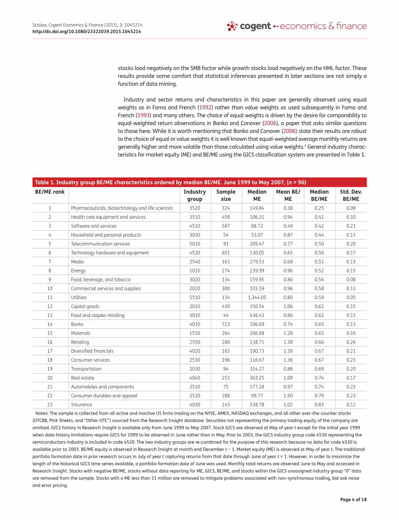
Industry and sector returns and characteristics in this paper are generally observed using equal weights as in Fama and French (1992) rather than value weights as used subsequently in Fama and French (1993) and many others. The choice of equal weights is driven by the desire for comparability to equal-weighted return observations in Banko and Conover (2006), a paper that asks similar questions to those here. While it is worth mentioning that Banko and Conover (2006) state their results are robust to the choice of equal or value weights it is well known that equal-weighted average monthly returns are generally higher and more volatile than those calculated using value weights.3 General industry charac-teristics for market equity (ME) and BE/ME using the GICS classification system are presented in Table 1.

Table 1. Industry group BE/ME characteristics ordered by median BE/ME. June 1999 to May 2007, (n = 96)BE/ME rank Industry

groupSample

sizeMedian

MEMean BE/

MEMedian BE/ME

Std. Dev. BE/ME

1 Pharmaceuticals, biotechnology and life sciences 3520 324 149.84 0.38 0.25 0.08

2 Health care equipment and services 3510 458 106.31 0.94 0.41 0.10

3 Software and services 4510 587 88.72 0.49 0.42 0.21

4 Household and personal products 3030 54 53.07 0.87 0.44 0.13

5 Telecommunication services 5010 93 209.47 0.77 0.50 0.20

6 Technology hardware and equipment 4520 651 130.05 0.65 0.50 0.17

7 Media 2540 161 279.53 0.68 0.51 0.13

8 Energy 1010 274 239.99 0.96 0.52 0.15

9 Food, beverage, and tobacco 3020 134 159.95 0.86 0.56 0.08

10 Commercial services and supplies 2020 300 103.59 0.96 0.58 0.13

11 Utilities 5510 134 1,344.05 0.80 0.59 0.05

12 Capital goods 2010 430 150.54 1.06 0.62 0.15

13 Food and staples retailing 3010 44 436.43 0.86 0.62 0.13

14 Banks 4010 723 106.69 0.74 0.65 0.13

15 Materials 1510 264 206.88 1.28 0.65 0.16

16 Retailing 2550 280 238.71 1.38 0.66 0.26

17 Diversified financials 4020 165 190.73 1.39 0.67 0.21

18 Consumer services 2530 196 116.67 1.36 0.67 0.23

19 Transportation 2030 94 314.27 0.88 0.69 0.20

20 Real estate 4040 251 363.25 1.09 0.74 0.17

21 Automobiles and components 2510 75 177.28 0.97 0.74 0.23

22 Consumer durables and apparel 2520 288 99.77 1.50 0.79 0.23

23 Insurance 4030 143 538.78 1.02 0.83 0.12

Notes: The sample is collected from all active and inactive US firms trading on the NYSE, AMEX, NASDAQ exchanges, and all other over-the-counter stocks (OTCBB, Pink Sheets, and “Other-OTC”) sourced from the Research Insight database. Securities not representing the primary trading equity of the company are omitted. GICS history in Research Insight is available only from June 1999 to May 2007. Stock GICS are observed at May of year t except for the initial year 1999 when data history limitations require GICS for 1999 to be observed in June rather than in May. Prior to 2003, the GICS industry group code 4530 representing the semiconductors industry is included in code 4520. The two industry groups are re-combined for the purpose of this research because no data for code 4530 is available prior to 2003. BE/ME equity is observed in Research Insight at month end December t − 1. Market equity (ME) is observed at May of year t. The traditional portfolio formation date in prior research occurs in July of year t capturing returns from that date through June of year t + 1. However, in order to maximize the length of the historical GICS time series available, a portfolio formation date of June was used. Monthly total returns are observed June to May and accessed in Research Insight. Stocks with negative BE/ME, stocks without data reporting for ME, GICS, BE/ME, and stocks within the GICS unassigned industry group “0” data are removed from the sample. Stocks with a ME less than $1 million are removed to mitigate problems associated with non-synchronous trading, bid-ask noise and error pricing.

of 18


Unsurprisingly, results in Table 1 show that biotechnology, health care, software, telecommunica-tions, and technology industry groups—those typically found in growth-oriented mutual fund port-folios—are found in the growth end of the BE/ME ranking when ordered by median BE/ME across the sample period. It is again unsurprising that industries exhibiting high BE/ME characteristics shown in Table 1 are the same as those most found in the value-oriented Franklin Templeton Mutual Shares fund ($16 billion in net assets). At 31 December 2014, the fund held almost a quarter of its portfolio (23%) in financial stocks.4

Cohen and Polk (1996) suggest that an industry group or sector may exhibit consistently high BE/ME characteristics over time. The authors argue that a persistently high BE/ME characteristic may result from a unique accounting standard or the industry may simply be a riskier industry than oth-ers. Conversely, an industry whose BE/ME characteristic migrates from low to high may simply be under temporary distress. Insurance, transportation, financial, and consumer durables are observed in the high end of the median BE/ME ordering in Table 1. However, variation in BE/ME characteristics, computed as the standard deviation of the observed eight-year time series and presented in the last column of Table 1, is large enough to warrant caution by value investors in allocating funds based on the historical median BE/ME of these industry groups.

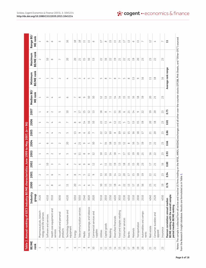
Table 2 shows the temporal consistency of the annual median BE/ME ranking of GICS industry groupings, similar to the presentation in Banko and Conover (2006) who use SIC sorted groupings. Although periodic ranking migration does occur, specifically the energy and telecommunications industries, the overall temporal consistency in BE/ME ranking is fairly high. Pharmaceuticals exhibit the lowest relative median BE/ME characteristic for all but one of the eight years in the sample period while the insurance industry exhibits the highest median BE/ME characteristic in five of the eight years of the sample. The Pearson correlation coefficient evaluating the degree of association between the annual BE/ME ranking and the aggregate median ranking over the entire sample period is greater than 0.66 for each of the eight years, and most of the annual coefficients are above 0.80. High positive correlations for the annual BE/ME rankings with the eight-year median for that industry are, of course, somewhat predictable given that the rankings are subsets of the aggregate data used to compute the median. However, the consistency of the resulting high correlations across time sug-gest that some predictability in observing industry ordering of BE/ME characteristics may be possible. Banko and Conover (2006) perform similar temporal consistency tests for 21 industries defined by SIC. The average range of BE/ME rank migration for each of their 21 industries is 14 places. This com-pares to an average annual range of BE/ME rank migration shown in the last column of Table 2 of only 11 places for the 23 industries defined by GICS (albeit for a shorter time period). The four lowest BE/ME ranked industries migrate on average only five places, suggesting that extreme growth-ori-ented industries exhibit some level of temporal BE/ME stability.

Fama and French (1997) observe HML factor loadings for 48 industry groupings using SIC codes and find that loadings vary considerably across industries and vary considerably across time. The authors find the results “distressing” with negative implications for any precise computation of a company’s cost of equity capital. Cohen and Polk (1996) and Nelson (2006) both attempt with some success to resolve the three-factor model’s difficulty in explaining returns when stocks are sorted by industry. Results from Banko and Conover (2006) are consistent with those from Cohen and Polk that the value effect is indeed found across industry groupings but at a much lower level of power than at the firm level.

For comparability, Table 3 shows equal-weighted monthly returns of GICS sorted industry groups regressed on the Fama–French three-factor model, June 1999 to May 2007. Results in Table 3 show that intercepts for equal-weighted excess industry returns are similarly problematic for the explanatory pow-er of the three-factor model. Four of twenty-three intercepts, or 17%, are statistically different from zero. This compares to 21% of intercepts using SIC codes in Fama and French (1997).5 As in earlier research, individual industry factor loadings for market, SMB, and HML are almost all statistically significant. Thus, model results when employing GICS codes for the present sample period are not materially different

of 18


Tabl

e 2.

Ann

ual r

anki

ng o

f GIC

S in

dust

ry B

E/M

E ch

arac

teris

tics.

June

199

9 to

May

200

7, (n

= 9

6)BE

/ME

rank

Indu

stry

gr

oup

2000

2001

2002

2003

2004

2005

2006

2007

Med

ian

BE/

ME

rank

Min

imum

BE

/ME

rank

Max

imum

BE

/ME

rank

Rang

e BE

/M

E ra

nk 1

Phar

mac

eutic

als,

bio

tech

-no

logy

and

life

sci

ence

s35

201

21

11

11

11

12

1

2So

ftw

are

and

serv

ices

4510

21

103

63

24

31

109

3He

alth

car

e eq

uipm

ent a

nd

serv

ices

3510

86

32

34

42

42

86

4Ho

useh

old

and

pers

onal

pr

oduc

ts30

305

77

42

23

55

27

5

5Te

chno

logy

har

dwar

e an

d eq

uipm

ent

4520

114

45

205

710

64

2016

6En

ergy

1010

208

26

413

83

72

2018

7Te

leco

mm

unic

atio

n se

rvic

es50

103

36

1121

96

178

321

18

8M

edia

2540

45

98

96

1415

94

1511

9Fo

od, b

ever

age,

and

toba

cco

3020

611

89

514

1612

105

1611

10Co

mm

erci

al s

ervi

ces

and

supp

lies

2020

79

1212

107

1013

107

136

11Ut

ilitie

s55

1010

135

107

2222

1812

522

17

12Ca

pita

l goo

ds20

1015

1611

1314

1211

813

816

8

13Re

tailin

g25

5012

1022

1418

109

711

722

15

14Di

vers

ified

fina

ncia

ls40

2018

1419

1813

812

1114

819

11

15Fo

od a

nd s

tapl

es re

tailin

g30

109

1213

715

1921

1614

721

14

16Co

nsum

er s

ervi

ces

2530

2220

1817

1211

56

155

2217

17Ba

nks

4010

1317

1415

815

1721

158

2113

18M

ater

ials

1510

1715

1519

1616

1314

1613

196

19Tr

ansp

orta

tion

2030

1418

2020

1718

159

189

2011

20Au

tom

obile

s an

d co

mpo

-ne

nts

2510

1619

2321

1917

1922

1916

237

21Re

al e

stat

e40

4023

2217

1611

2120

1920

1123

12

22Co

nsum

er d

urab

les

and

appa

rel

2520

2121

2122

2220

1820

2118

224

23In

sura

nce

4030

1923

1623

2323

2323

2316

237

Pear

son

corr

elat

ion:

ann

ual m

edia

n BE

/ME

rank

ing

with

the

over

all s

ampl

e pe

riod

med

ian

BE/M

E ra

nkin

g

0.76

0.94

0.80

0.93

0.66

0.86

0.81

0.75

Aver

age

rank

rang

e11

Not

es: T

he s

ampl

e is

col

lect

ed fr

om a

ll ac

tive

and

inac

tive

US

firm

s tr

adin

g on

the

NYS

E, A

MEX

, NAS

DAQ

exc

hang

es a

nd a

ll ot

her o

ver-

the-

coun

ter s

tock

s (O

TCBB

, Pin

k Sh

eets

, and

“O

ther

-OTC

”) s

ourc

ed

from

the

Rese

arch

Insi

ght d

atab

ase.

Res

ults

are

form

ulat

ed a

s in

Tab

le 1

.

of 18


from those when sorting stocks by SIC codes for earlier periods.6 For investors, HML loadings shown in Table 3 generally confirm the growth (risk) orientation of industry groups such as pharmaceuticals (−0.68, t = −2.96) compared to the value (risk) orientation of industry groups such as insurance (0.63, t = 7.83). HML risk loadings are also generally consistent with the rank order of median BE/ME. The Pearson correlation between median BE/ME characteristics and HML factor loadings is 0.70 (t = 3.07). While correlation results are generally unsurprising since HML is itself crafted from BE/ME rankings, the consistency and predictability of results in Table 3 are nevertheless helpful to investors who may attempt to capture a risk-based value premium by observing industry BE/ME accounting statistics.

Table 3. Equal-weighted excess monthly returns of GICS sorted industry groups regressed on the Fama–French three-factor model. June 1999 to May 2007, (n = 96)

BE/ME rank

GICS industry group Code Median BE/ME

a b s h t(a) t(b) t(s) t(h) R2

1 Pharmaceuticals, etc. 3520 0.25 1.59 0.92 1.55 −0.68 (2.49)* (3.80)* (4.51)* (−2.96)* 0.69

2 Health care equipment and services

3510 0.41 0.82 0.84 0.94 0.25 (1.86) (6.61)* (6.62)* (1.92) 0.62

3 Software and services 4510 0.42 1.22 1.49 0.90 −0.84 (1.72) (10.21)* (4.45)* (−3.49)* 0.72

4 Household and personal products

3030 0.44 0.64 0.66 0.55 0.25 (1.26) (5.04)* (4.30)* (1.33) 0.35

5 Telecommunication services

5010 0.50 0.62 1.27 0.71 −0.37 (1.03) (7.00)* (4.39)* (−1.92) 0.63

6 Technology hardware and equipment

4520 0.50 1.03 1.55 1.17 −0.47 (1.93) (9.10)* (6.32)* (−2.94)* 0.80

7 Media 2540 0.51 −0.11 1.12 0.48 −0.05 (−0.22) (9.59)* (3.50)* (−0.36) 0.62

8 Energy 1010 0.52 1.49 0.97 0.48 0.80 (2.55)* (5.50)* (2.86)* (4.41)* 0.32

9 Food, beverage, and tobacco

3020 0.56 0.56 0.50 0.45 0.53 (1.79) (7.25)* (5.43)* (5.16)* 0.37

10 Commercial services and supplies

2020 0.58 0.40 0.93 0.61 0.34 (0.93) (10.96)* (5.62)* (2.66)* 0.55

11 Utilities 5510 0.59 0.18 0.60 0.22 0.75 (0.67) (7.02)* (3.43)* (8.61)* 0.51

12 Capital goods 2010 0.62 0.85 0.99 0.58 0.37 (2.26)* (11.56)* (5.57)* (2.96)* 0.65

13 Food and staples retail-ing

3010 0.62 −0.08 0.78 0.44 0.59 (−0.24) (8.52)* (4.75)* (4.80)* 0.50

14 Banks 4010 0.65 0.45 0.38 0.22 0.48 (1.98) (7.59)* (2.95)* (6.31)* 0.38

15 Materials 1510 0.65 0.30 1.08 0.53 0.72 (0.89) (14.17)* (5.30)* (6.50)* 0.66

16 Retailing 2550 0.66 0.21 1.07 0.60 0.42 (0.40) (9.63)* (3.55)* (2.15)* 0.48

17 Diversified financials 4020 0.67 1.05 0.98 0.53 0.19 (2.48)* (9.98)* (4.96)* (1.44) 0.59

18 Consumer services 2530 0.67 0.55 0.78 0.62 0.53 (1.39) (8.71)* (5.59)* (3.55)* 0.50

19 Transportation 2030 0.69 0.31 1.12 0.45 0.66 (0.63) (8.95)* (3.34)* (4.34)* 0.52

20 Real estate 4040 0.74 0.52 0.42 0.37 0.50 (1.86) (7.32)* (5.11)* (5.83)* 0.42

21 Automobiles and com-ponents

2510 0.74 −0.37 1.09 0.55 0.67 (−0.69) (8.98)* (3.89)* (3.82)* 0.46

22 Consumer durables and apparel

2520 0.79 0.05 0.99 0.54 0.57 (0.12) (11.45)* (4.70)* (4.27)* 0.59

23 Insurance 4030 0.83 0.28 0.77 0.18 0.63 (1.14) (11.84)* (2.63)* (7.83)* 0.62

Pearson correlation with Median BE/ME −0.64 −0.23 −0.73 0.70

t-Stat. (−2.82)* (−1.05) (−3.15)* (3.07)*

Notes: Industry t-statistic use heteroskedasticity-consistent errors.*t-Statistic significant at the 5% level.

Rpt − Rft = a + b[Rmt − Rft] + sSMBt + hHMLt + et

of 18


Figure 1 provides further information on the consistency of BE/ME characteristics that may be beneficial for investment professionals seeking to allocate funds across industry groups. For this presentation, all NYSE, AMEX, NASDAQ, and all “other” OTC stocks are annually sorted into BE/ME

Figure 1. Average annual percentage of GICS industry group stocks appearing in various BE/ME quintiles, June 1999 to May 2007 (n = 96).

of 18


quintiles. GICS industry codes are next observed for stocks within each quintile for each year in the sample and then averaged across time for each industry. Chart A shows that on average approxi-mately 60% of pharmaceutical stocks are found in the lowest BE/ME quintile across the entire sam-ple period.

This compares to less than 10% of insurance stocks found in that same growth-oriented quintile. Industry allocations across the middle 2nd, 3rd, and 4th quintiles are fairly evenly distributed with two exceptions. The largest portion of utility and bank stocks are found in the middle quintile in Chart C. This is somewhat surprising given the tendency of value investment managers to allocate large portions of their portfolios to these industry groups. This observation may hint to a reason why Houge and Loughran (2006) find that value managers have generally failed to capture the statistical rewards of the value premium as promised in the academic literature. Chart E, reflecting the highest BE/ME value-oriented stocks, again show predictable contents. On average, over 30% of insurance, consumer durables, and automobile stocks are found in this extreme BE/ME quintile over the sample period. Results from Figure 1 show that stocks from growth-oriented industries tend to cluster at high rates in the lowest BE/ME quintile while stocks from value-oriented industries are more evenly distributed across the middle quintiles. This hints that the computed value premium in returns for stocks occupying the highest BE/ME quintile is driven from a more equitable distribution of industry groups.

Results from Tables 1 and 2 as well as Figure 1 suggest that value investors using a top-down/bottom-up method may be able to avoid the relatively inferior returns of low BE/ME firms by avoiding certain industry groups, but investors may not be able to capture the superior returns of high BE/ME stocks by exclusively allocating to industry groups historically exhibiting a high BE/ME characteristic. Results showing the temporal stability of growth industry BE/ME and relative temporal instability of value industry BE/ME are consistent with findings in Banko and Conover (2006) of the relatively weaker power of an across-industry effect.

Results in both Table 2 and from the various quintile charts in Figure 1 suggest that certain industries have a natural or structural tendency with respect to BE/ME characteristics. Technology stocks appear to generally exhibit low BE/ME fundamental characteristics while Insurance stocks appear to generally exhibit high BE/ME fundamental characteristics. Growth fund managers who exclusively screen compa-nies based on low BE/ME characteristics may find their portfolios disproportionately weighted with technology industry stocks over time. Conversely, value managers who exclusively screen companies based on high BE/ME characteristics may find their portfolios disproportionately weighted with insur-ance stocks.

4. The value premium across industry sectorsChen and Zhang (1998) find that stocks in certain developing economies like Thailand and Taiwan do not exhibit a value premium. They argue this is due to high economic growth conditions and there-fore a lack of overall market distress. If Chen and Zhang are correct, then high BE/ME value stocks found within (distressed) value industries should exhibit superior performance to high BE/ME value stocks found within (less distressed) growth industries. Banko and Conover (2006) test this thesis in a cross-industry analysis and find that value firms in value industries do indeed generate superior returns to value firms in growth industries, consistent with predictions of Chen and Zhang.

The performance of value and growth stocks within each GICS industry group are next examined to determine whether value stocks in value industries indeed generate higher relative returns. The question is motivated not by prior findings related to the pricing of distress risk, but instead by the needs of top-down/bottom-up value investors who wish to find predictable patterns of value pre-mium behavior within and across industry groupings. Portfolios are formed first by sorting stocks by GICS industry sector and then independently sorting NYSE, AMEX, NASDAQ, and all other OTC stocks 2 × 5 by size and BE/ME, using the method in Fama and French (1993). The precise portfolio construc-tion methodology is again detailed in the notes of Table 1.

of 18


In this examination, sample size restrictions force the use of broader two-digit GICS industry clas-sifications rather than four. The two-digit code represents a more macro combination of the various 23 GICS industry groupings (see Appendix A for a map of the GICS classification system). Ideally, within-industry performance of the entire set of 23 GICS industry groups would be evaluated to cre-ate a finer cut of performance differentiation. However, the use of industry (or economic) sectors rather than industry groups allows for tests of larger samples through time and therefore better statistical inferences from those samples. Larger sample sizes also allow for the use of controls for size and greater differentiation within BE/ME characteristics.7 Banko and Conover (2006) apparently experience similar problems with industry sample sizes. Their solution is to create generic groups of low BE/ME growth industry portfolios and generic groups of high BE/ME value portfolios—thus elimi-nating industry and sector identities altogether.

To ensure proper statistical inferences, all econometric tests using industry sectors in this paper require a fifteen stock minimum portfolio sample when independently sorting 2 × 5 on size and BE/ME, thus following standards established in Banko and Conover (2006) for similar tests. This restriction results in the exclusion of two sectors, telecom (GICS code 50, n = 8) and utilities (GICS code 55, n = 13). The only requirement for an evaluation of within-sector and across-sector returns and risk characteristics is that remaining sectors reflect substantial variation across BE/ME characteristics. Such variation in the BE/ME characteristic will allow a proper delineation between value-oriented sectors and growth-oriented sectors. Indeed, median BE/ME characteristics for financials in the remaining sample (0.72) are more than double the median BE/ME characteristic for health care (0.33).

Table 4 shows the average equal-weighted monthly return of GICS sector portfolios sorted inde-pendently 2 × 5 on size and BE/ME. Stocks are first sorted into one of the eight GICS sectors. Then, within each sector, stocks are sorted by size at a breakpoint above and below $491 million. The breakpoint is derived using the average of the Fama and French ME breakpoints for the 25th percen-tile over the eight-year period, June 1999 to May 2007. A fixed breakpoint over time is preferred rather than a floating or relative annual ME or BE/ME breakpoint because it establishes fixed charac-teristics for specific levels of ME and BE/ME. Testing stocks below and above the 25th percentile helps in three ways. First, small stocks dominate the sample; therefore, skewing the size breakpoint to 25%/75% creates samples large enough to test large-cap stocks within each economic sector. Second, the value premium has been shown to predominate in the small-cap stratum of stocks. If the value premium is present within and across economic sectors, it is more likely to be found below a portfolio market capitalization of $491 million and less likely above it. Third, because of liquidity constraints and other trading difficulties, $491 million in individual stock market capitalization rep-resents a level below which most institutional investors rarely invest. Therefore, results for stocks above the $491 million market-cap would be informative regarding the question of any institutional investor’s ability to capture the value premium.8 Following the sort for size, stocks are further sorted into quintiles using the Fama and French 20th, 40th, 60th, and 80th percentile BE/ME breakpoints averaged over the sample period. Stocks are sorted and rebalanced annually as before. Portfolio returns in Panel A of Table 4 are computed as equal-weighted arithmetic averages of monthly returns across stocks in the sample. Returns reflect the average of monthly returns for each quintile over the eight-year sample period (n = 96). Returns in Panel A can be defined as the average monthly return for various size and BE/ME portfolios over the eight-year sample period.

Certain portfolio returns shown in Panel A, namely returns for stocks larger than the ME break-point, suffer some degree of noise due to relatively small number of stocks in the portfolio. For fur-ther confidence in results, returns are computed using a different method. Panel B shows returns for stocks sorted by sector and then 2 × 5 on size and BE/ME as before. However, returns in this presen-tation are averaged across time rather than creating a 96 month time series of portfolio returns. Data presented in Panel B can be defined as average monthly returns for the average stock in a specific size and BE/ME strata in a specific sector. For example, it can be said that on average, each stock in the small-cap LO BE/ME health care portfolio returned 1.92% per month between June 1999 and May 2007.

of 18


Results are summarized as follows: The HI-minus-LO value premium shown in Panel A of Table 4 is statistically significant within all sectors below the size breakpoint, with the exception of finan-cials.9 In Panel B, five of the HI-LO quintile sector returns below the 25th size percentile are statisti-cally significant at the 5% level and the remaining three at the 10% level. Results in Panels A and B demonstrate that the value premium is clearly more pronounced in small and micro-cap stocks. The premium is statistically non-existent (often negative) within each sector above the size breakpoint of both panels A and B. Observing the value premium in only small-cap stocks is consistent with find-ings in Loughran (1997) and problematic for the specification of the three-factor model. Fama and French (2006), in an attempt to remedy the challenge from Loughran, argue that the weakness of the value premium in large stocks is unique to Loughran’s sample period 1963–1995 and unique to US stocks. Results in Table 4, using a sample subsequent to the period tested by Loughran, certainly undermines the argument that the weakness is sample specific.

Banko and Conover (2006) observe that growth stocks in value industries have superior returns to growth stocks in growth industries. Further, value stocks in value industries have superior returns to value stocks in growth industries. Both observations are inconsistent with results in Table 4.10 For small-cap stocks, low BE/ME growth stocks in growth industries have superior returns to low BE/ME growth stocks in value industries. High BE/ME value stocks in growth industries outperform high BE/ME value stocks in value industries.

Table 4. Average portfolio returns for stocks sorted by GICS industry sector and then 2 × 5 on size and BE/ME. June 1999 to May 2007, (n = 96)

Below ME breakpoint of $491 million Above ME breakpoint of $491 millionBook to market equity Book to market equity

Sector GICS BE/ME LO 2 3 4 HI HI-LO t-Stat. LO 2 3 4 HI HI-LO t-Stat.Panel A: Monthly time series of portfolio returns

Health care 35 0.33 2.09 2.49 2.37 3.06 4.05 1.96 (3.45)* 1.26 1.72 1.70 1.36 1.03 −0.24 (−0.20)

Info. Tech. 45 0.46 1.60 2.19 3.00 2.28 3.07 1.48 (2.41)* 1.10 1.43 1.64 1.76 0.78 −0.31 (−0.39)

Energy 10 0.52 2.65 2.25 2.87 3.28 4.72 2.07 (2.23)* 2.17 2.05 2.38 2.05 1.41 −0.76 (−0.82)

Cons. Staples 30 0.54 1.09 1.69 1.54 1.39 2.79 1.69 (2.35)* 1.02 0.94 0.91 1.70 1.43 0.41 (0.17)

Industrials 20 0.63 1.24 1.62 1.76 1.92 2.44 1.20 (2.27)* 1.01 1.35 1.24 1.23 0.61 −0.40 (−0.63)

Materials 15 0.65 0.93 1.73 0.62 1.62 2.55 1.62 (2.06)* 1.10 1.49 1.24 1.89 2.38 1.27 (1.54)

Cons. Discr. 25 0.67 0.80 1.49 1.28 1.36 1.95 1.15 (2.62)* 0.91 0.94 0.91 1.11 1.36 0.45 (0.93)

Financials 40 0.72 1.23 1.32 1.20 1.39 1.73 0.50 (1.00) 1.03 1.21 1.13 1.40 1.16 0.13 (0.34)

Average 1.45 1.85 1.83 2.04 2.91 1.46 1.20 1.39 1.39 1.56 1.27 0.07

Pearson correlation: BE/ME with HI-LO returns

−0.74 (−2.69)* 0.46 (1.26)

Panel B: Portfolio returns averaged across time

Health care 35 0.33 1.92 2.56 2.54 3.58 4.58 2.66 (4.51)* 1.09 1.63 1.63 1.93 1.62 0.53 (0.64)

Info. Tech. 45 0.46 1.20 2.27 3.13 2.66 3.84 2.65 (2.32)* 0.69 1.27 1.31 1.72 0.87 0.18 (0.12)

Energy 10 0.52 2.45 2.23 2.82 3.21 4.69 2.24 (2.29)* 1.64 2.11 2.48 2.44 2.47 0.84 (0.86)

Cons. Staples 30 0.54 0.92 1.46 1.61 1.14 2.76 1.84 (2.88)* 0.89 0.85 1.09 1.96 2.60 1.71 (1.29)

Industrials 20 0.63 1.28 1.45 1.73 1.84 2.29 1.01 (1.82) 1.01 1.41 1.31 1.46 1.14 0.13 (0.18)

Materials 15 0.65 1.08 1.76 0.69 1.37 2.39 1.31 (1.87) 1.22 1.56 1.26 1.18 2.44 1.21 (1.07)

Cons. Discr. 25 0.67 0.60 1.30 1.16 1.28 2.00 1.40 (2.52)* 0.84 0.90 0.86 1.31 1.67 0.83 (1.30)

Financials 40 0.72 1.27 1.12 1.10 1.50 2.07 0.80 (1.85) 1.05 1.14 1.10 1.43 1.45 0.40 (1.24)

Average 1.34 1.77 1.85 2.07 3.08 1.74 1.05 1.36 1.38 1.68 1.78 0.73

Pearson correlation: BE/ME with HI-LO returns

−0.93 (−6.03)* 0.08 (0.21)

*t-Statistic significant at the 5% level.

of 18


Table 4 shows that, while the within-industry value premium is apparently not subsumed by industry-specific influences, industry distinctions do remain. During this sample period, the value premium is remarkably stronger in growth sectors such as health care (1.96% per month) and information technol-ogy (1.48% per month), and weaker in value sectors such as financials (0.50% per month) and con-sumer discretionary (1.15% per month). Pearson correlation coefficients for HI-LO returns and median BE/ME characteristics across the eight economic sectors confirm the association between a large value premium and low BE/ME characteristics. Coefficients shown in Panel A of Table 4 are strong and nega-tive for stocks below the 25th size percentile (ρ = −0.74, t = 2.69). However, no statistically significant association between the value premium and a sector’s BE/ME ranking is observed in large-cap stocks above the 25th size percentile (ρ = 0.46, t = 1.26). Although the sign is notably positive.

Results in Table 4 Panel B provide clear contrast to prior findings that the value premium is stronger in value-oriented industries. The HI-LO statistic for small-cap stocks in Panel B is almost perfectly monotonic, falling as median BE/ME rises across eight industry sectors (ρ = −0.94, t = −6.90). Contradictory evidence between prior published results and those in Table 4 is not helpful to value investors who seek to capture the value premium using a macro industry approach. To capture the value premium, an investor needs to be highly confident the premium will be consistent in size and predictable in location.

5. January anomaly and the value premium within and across industry sectorsThe January anomaly in returns is a well-documented challenge to the theory of efficient markets. Rozeff and Kinney (1976) initially observe the anomaly in equal-weighted NYSE returns, and the phe-nomenon is confirmed in Reinganum (1983) and Roll (1983) showing the effect to predominate in small stocks. Lakonishok and Smidt (1988) find the January anomaly to persist over their 90-year sample period of daily data. Explanations for the effect have ranged from end-of-year window dress-ing by institutional investors to individual tax loss selling.11 Haug and Hirschey (2006) update research on the January effect to test its existence subsequent to the enactment of the Tax Reform Act of 1986, a tax law that materially impacted mutual fund capital gain distributions. The authors find a persistent January effect in equal-weighted returns in small-cap stocks despite the change in tax law.

The question for this research is whether the January anomaly in returns subsumes or impacts the value premium in industry sectors that are shown in Table 4. As a practical matter, if the value premi-um is subsumed by the January anomaly within and across industry sectors, then investors who make industry allocations within their portfolios need only to concentrate on the January premium rather than the BE/ME premium in their attempt to capture superior returns over time. In addition to docu-menting the January return premium across and within GICS industry groupings, this research seeks to shed further light on Loughran (1997) who argues that the BE/ME premium is driven in large part, first by low returns of growth stocks in the 11 months excluding January and second by returns associated with the January anomaly. This section asks, (1) Does the January premium in returns exist within each GICS industry sector using a sample period subsequent to the US Tax Reform Act of 1986, and more importantly, (2) If a January anomaly exists in this data, do value premium characteristics in equal-weighted returns observed in Table 4 survive after re-testing only the 11 months excluding January?

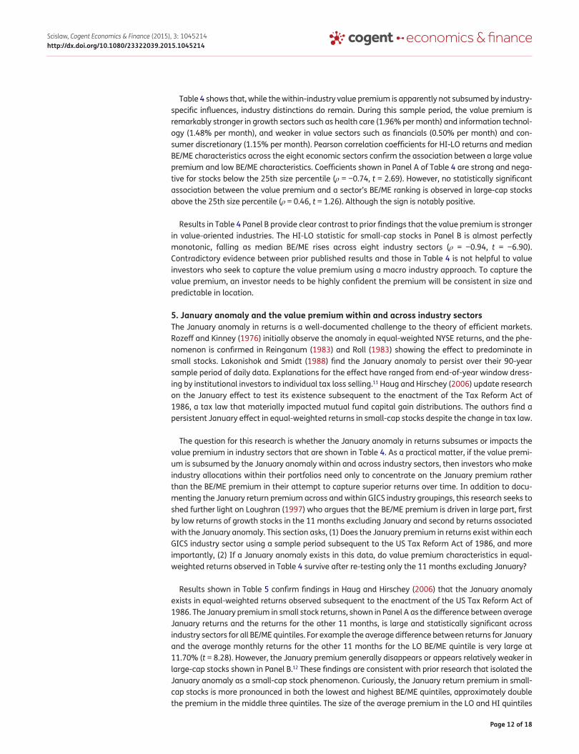
Results shown in Table 5 confirm findings in Haug and Hirschey (2006) that the January anomaly exists in equal-weighted returns observed subsequent to the enactment of the US Tax Reform Act of 1986. The January premium in small stock returns, shown in Panel A as the difference between average January returns and the returns for the other 11 months, is large and statistically significant across industry sectors for all BE/ME quintiles. For example the average difference between returns for January and the average monthly returns for the other 11 months for the LO BE/ME quintile is very large at 11.70% (t = 8.28). However, the January premium generally disappears or appears relatively weaker in large-cap stocks shown in Panel B.12 These findings are consistent with prior research that isolated the January anomaly as a small-cap stock phenomenon. Curiously, the January return premium in small-cap stocks is more pronounced in both the lowest and highest BE/ME quintiles, approximately double the premium in the middle three quintiles. The size of the average premium in the LO and HI quintiles

of 18


Tabl

e 5.

Ave

rage

Jan

uary

retu

rns

and

aver

age

mon

thly

retu

rns

excl

udin

g Ja

nuar

y fo

r sec

tor p

ortf

olio

s so

rted

2 ×

5 fo

r siz

e an

d BE

/ME.

Jun

e 19

99 to

May

200

7Bo

ok to

mar

ket q

uint

iles

(BE/

ME)

LO2

34

HIPa

nel A

: Sm

all S

tock

s

Sect

orJa

nuar

y11

Mos

.Di

ffere

nce

Janu

ary

11 M

os.

Diffe

renc

eJa

nuar

y11

Mos

.Di

ffere

nce

Janu

ary

11 M

os.

Diffe

renc

eJa

nuar

y11

Mos

.Di

ffere

nce

Heal

th c

are

11.5

61.

0410

.51

12.4

81.

6610

.82

11.8

01.

6910

.11

13.4

72.

6810

.79

16.5

13.

5013

.02

Info

. Tec

h.19

.04

−0.4

319

.47

12.9

41.

2911

.65

11.2

72.

398.

8811

.53

1.86

9.67

16.5

12.

6913

.82

Ener

gy7.

921.

965.

965.

821.

903.

924.

982.

622.

364.

893.

061.

8315

.36

3.72

11.6

4

Cons

. Sta

ples

12.4

1−0

.12

12.5

24.

761.

163.

607.

751.

056.

704.

690.

823.

8711

.62

1.96

9.67

Indu

stria

ls12

.27

0.28

11.9

95.

751.

064.

696.

401.

315.

096.

651.

405.

2512

.00

1.41

10.5

9

Mat

eria

ls12

.25

0.06

12.1

96.

631.

325.

315.

410.

275.

145.

381.

004.

3812

.27

1.49

10.7

9

Cons

. Disc

r.12

.54

−0.4

813

.02

8.14

0.68

7.46

6.28

0.70

5.58

7.95

0.67

7.28

12.2

71.

0711

.20

Finan

cial

s8.

520.

617.

922.

461.

001.

461.

901.

030.

863.

011.

361.

656.

441.

674.

77

Aver

age

12.0

60.

3611

.70

7.37

1.26

6.11

6.97

1.38

5.59

7.20

1.61

5.59

12.8

72.

1910

.69

t-St

at.

(8

.28)

*

(4.8

2)*

(5

.16)

*

(4.6

5)*

(1

1.04

)*

Pane

l B: L

arge

Sto

cks

Heal

th c

are

0.39

1.15

−0.7

60.

981.

69−0

.72

0.77

1.71

−0.9

32.

681.

860.

822.

051.

580.

47

Info

. Tec

h.6.

640.

156.

491.

251.

28−0

.03

2.68

1.19

1.49

8.00

1.15

6.84

6.44

0.37

6.07

Ener

gy1.

821.

620.

191.

502.

17−0

.67

2.89

2.44

0.45

0.16

2.65

−2.4

94.

862.

262.

60

Cons

. Sta

ples

0.64

0.92

−0.2

8−1

.48

1.06

−2.5

50.

191.

17−0

.98

1.03

2.05

−1.0

210

.30

1.90

8.40

Indu

stria

ls−0

.17

1.12

−1.3

00.

201.

51−1

.31

0.06

1.42

−1.3

6−0

.33

1.63

−1.9

61.

341.

120.

22

Mat

eria

ls0.

611.

28−0

.67

1.30

1.58

−0.2

8−0

.12

1.39

−1.5

1−1

.41

1.42

−2.8

35.

052.

202.

86

Cons

. Disc

r.1.

300.

800.

500.

920.

900.

011.

000.

850.

161.

011.

33−0

.32

2.23

1.62

0.61

Finan

cial

s0.

871.

06−0

.19

−0.4

71.

29−1

.76

−0.3

41.

23−1

.57

−0.0

21.

56−1

.58

0.27

1.55

−1.2

8

Aver

age

1.51

1.01

0.50

0.52

1.44

−0.9

10.

891.

42−0

.53

1.39

1.71

−0.3

24.

071.

582.

49

t-St

at.

(0

.57)

(−

2.86

)*

(−1.

35)

(−

0.29

)

(2.1

6)*

*t-S

tatis

tic s

igni

fican

t at t

he 5

% le

vel.

of 18


is 11.70 and 10.69%, respectively. Surprisingly, returns for the month of January, as well as differences between returns within each industry sector shown in Panel A of Table 5, appear larger for growth industry sectors than for value industry sectors. For example, the difference in returns across all BE/ME quintiles for the health care sector averages over 10% while the difference across BE/ME quintiles for the financial sector averages just over 3%. The ordering of differences is considerably more monotonic when viewing quintiles 2, 3, and 4.

A critical question remains whether the value premium as shown previously in Table 4 continues to survive once the January premium is removed from the sample. If the value premium is independ-ent of the January anomaly, then superior returns for high BE/ME stocks should still persist in aver-age portfolio returns when testing only the other 11 months of the calendar year. To examine this question, stocks are once again sorted 2 × 5 on size and BE/ME as before. Returns are again captured over the eight-year period June 1999 to May 2007 and computed in the manner presented in Panel B of Table 4.

Return observations for the month of January are excluded for each size and BE/ME portfolio and outcomes presented in Table 6. Results show that the value premium is robust even after removing the superior returns generated during the month of January—consistent with findings in Daniel and Titman (1997) who find the value effect to be independent of the January anomaly. Removing returns for the month of January does not materially impact the relative HI-LO value premium relationship. The key across-sector value premium characteristics shown previously in Table 4, critical to inferences related to stability and risk made in earlier sections of this paper, survive. The value premium remains more pronounced in growth sectors than in value sectors during this sample period even when returns for the month of January are omitted. Sector HI-LO premiums continue to be highly negatively correlated with the median sector BE/ME characteristics for small stocks (ρ = −0.81, t = −3.40). The premium is statisti-cally significant for small-cap stocks at the 5% level within five of eight industry sectors and significant at the 10% level within the remaining three—a result similar to within-sector premiums observed earlier in Table 4. After omitting returns for the month of January, the value premium continues to be non-existent in large-cap stocks. None of the HI-LO computations are large and statistically different from zero. Moreover, correlations between sector HI-LO premiums and sector BE/ME characteristics in large-cap stocks are indistinguishable from zero (ρ = 0.22, t = 0.55), reflecting no association between the computed premia and the ordering of sector BE/ME characteristics.

Table 6. Average monthly GICS industry sector portfolio returns for stocks sorted 2 × 5 on size and BE/ME, excluding returns for the month of January. June 1999 to May 2007, (n = 88)

Below ME breakpoint of $491 million Above ME breakpoint of $491 millionBook to market equity Book to market equity

Sector GICS BE/ME LO 2 3 4 HI HI-LO

t-Stat. LO 2 3 4 HI HI-LO

t-Stat.

Health care 35 0.33 1.04 1.66 1.69 2.68 3.50 2.45 (4.06)* 1.15 1.69 1.71 1.86 1.58 0.43 (0.47)

Info. Tech. 45 0.46 −0.43 1.29 2.39 1.86 2.69 3.12 (2.74)* 0.15 1.28 1.19 1.15 0.37 0.22 (0.13)

Energy 10 0.52 1.96 1.90 2.62 3.06 3.72 1.76 (1.89) 1.62 2.17 2.44 2.65 2.26 0.64 (0.61)

Cons. Staples 30 0.54 −0.12 1.16 1.05 0.82 1.96 2.08 (3.20)* 0.92 1.06 1.17 2.05 1.90 0.99 (0.81)

Industrials 20 0.63 0.28 1.06 1.31 1.40 1.41 1.13 (1.89) 1.12 1.51 1.42 1.63 1.12 0.00 (0.00)

Materials 15 0.65 0.06 1.32 0.27 1.00 1.49 1.43 (1.89) 1.28 1.58 1.39 1.42 2.20 0.92 (0.76)

Cons. Discr. 25 0.67 −0.48 0.68 0.70 0.67 1.07 1.55 (2.65)* 0.80 0.90 0.85 1.33 1.62 0.82 (1.17)

Financials 40 0.72 0.61 1.00 1.03 1.36 1.67 1.06 (2.81)* 1.06 1.29 1.23 1.56 1.55 0.49 (1.44)

Average 0.36 1.26 1.38 1.61 2.19 1.82 1.01 1.44 1.42 1.71 1.58 0.56

Pearson correlation: BE/ME with HI-LO returns −0.81 (−3.40)* 0.22 (0.55)

*t-Statistic significant at the 5% level.

of 18


Average monthly returns in Table 6, computed after excluding superior January returns, are by defini-tion smaller than those shown earlier in Panel B of Table 4. However, the average monthly HI-LO value premium in sector returns for small-cap stocks in Table 4 (1.74%) is almost identical to the premium for small stocks in Table 6 (1.82%). Results show that the average value premium computed across GICS industry sectors is not impacted by January returns—although slight variations in individual sector premia are naturally observed. Moreover, results in Table 6 (excluding January) when compared to those earlier in Table 4 (including January) do not suggest the value premium is stronger in the 11 months excluding the month of January as observed by Dhatt et al. (1999). Nor are results consistent with find-ings in Loughran (1997) that the value premium is boosted in part by January returns.

6. ConclusionThis paper helps to establish the body of research literature using the Global Industry Classification Standard, a system that Bhojraj et al. (2003) argues is superior for testing many industry-related research questions. Moreover, several important financial products are now constructed based on the GICS indus-try classification system. Any research attempting to reconcile academic research with market-based portfolios should use definitions and methods common and available to investors.

Results for a pre-financial collapse sample period show that GICS industry groups exhibit large differ-ences in BE/ME characteristics over the sample period; thus, potentially providing opportunities for inves-tors to capture the value premium in average returns by strategically allocating funds to targeted industry groups. Further, the annual ranking of industry BE/ME appears to be relatively stable and poten-tially predictable for investors. The four lowest BE/ME ranked industries migrate to higher BE/ME charac-teristics on average only five places, suggesting that extreme growth-oriented industries have considerable temporal BE/ME stability. Value-oriented industry groupings are less stable over the sample period. Stocks from growth-oriented industries tend to cluster at high rates in the lowest BE/ME quintile while stocks from value-oriented industries appear more evenly distributed across the middle BE/ME quintiles over time. This means that the relatively poor returns generated by low BE/ME growth stocks may largely originate in a few persistently poor performing growth-oriented industry groups. If growth industries (or sectors) consistently underperform value industries, then investors can use these temporal characteristics to allocate away from these industries. However, Table 4 shows the relationship to be more complex. During the sample period, high BE/ME value stocks residing in low BE/ME growth sectors actually outperform value stocks in value sectors.

The value premium is shown to disappear in large-cap stocks both within and across industry sec-tors. This finding is consistent with results in Loughran (1997) and problematic for the specification of the three-factor model as well as for a risk-based explanation to the BE/ME effect. Results in Table 4, using a sample period subsequent to that in Loughran (1997), appear to undermine the argument in Fama and French (2006) that Loughran’s observation of a weak value premium in large stocks is sample specific. This paper shows that the value premium is found to be statistically significant in all but one sector containing small-cap stocks and not statistically different from zero in all sectors con-taining large-cap stocks.

Using within-sector data and across-sector data, this paper provides additional evidence confirm-ing results in Haug and Hirschey (2006) who observe a strong January anomaly in more recent time periods. Results from within-sector tests of the value premium in Table 4 still survive once returns from the month of January are removed. Equally important, the across-sector association between sector BE/ME and the value premium in small-cap stocks remains statistically significant. Loughran (1997) argues that the BE/ME effect and the value premium are, in large part, driven by the January effect. However, results in Table 6 show that the average value premium computed across GICS industry sectors is not impacted by January returns. Results do not suggest the value premium is stronger in the 11 months, excluding the month of January, as observed by Dhatt et al. (1999). Nor are results consistent with findings in Loughran (1997) that the value premium is boosted in part by January returns.

of 18


FundingThe authors received no direct funding for this research.

Author detailsKenneth E. Scislaw1

E-mail: [email protected] ID: http://orcid.org/0000-0002-3753-92831 Breech School of Business, Drury University, 900 North

Benton Avenue, Springfield, MO 35801, USA.

Citation informationCite this article as: The value premium within and across GICS industry sectors in a pre-financial collapse sample, Kenneth E. Scislaw, Cogent Economics & Finance (2015), 3: 1045214.

Notes1. Chan, Lakonishok, and Swaminathan (2007) find that

both GICS and FF industry coding systems yield “sets of economically related stocks.” They compared GICS and FF systems with a mechanical industry clustering method, and find GICS and FF performs well in capturing out of sample return covariance as well as co-movement in fundamental characteristics such as sales growth.

2. The Standard & Poor’s Company uses GICS for its highly popular SPDR® exchange traded funds. S&P converted its ETF funds to the GICS system in June 2002. The giant Vanguard investment firm also uses GICS to classify stocks to their various sector ETFs. Internationally, several stock exchanges such as the Toronto, ASX in Australia, and Nordic exchanges use GICS for stock listing classifications. According to the sales literature produced by S&P, 8 of the top 10 sell-side investment firms and 9 of the 10 buy-side investment firms utilize the GICS sys-tem. The fact that Standard &Poor’s and Morgan Stanley own and manage the dominant S&P and MSCI global index products ensures that GICS will be heavily used by the practitioner community to construct any index-relat-ed industry sub-classifications. S&P announced that the conversion of their popular S&P/Citicorp equity growth and value indexes to GICS was completed in July 2005. Yet another popular classification system in wide use by practitioners is the Industry Classification Benchmark (ICB) by Dow Jones Indexes and FTSE. The popular Dow Jones I-Shares utilize the ICB classification system.

3. See Chiang (2002) for a comprehensive literature survey and analysis of the effect of statistical return weighting methods on the value effect.

4. Mutual fund portfolio holding data source: Morningstar.com.

5. When using the value-weighted return computation method employed by Fama and French, none of the intercepts are statistically significant. The average across-industry alpha of 0.30 for value-weighted returns is almost identical to the average absolute regression intercept of 0.28 across the 48 value-weight-ed industry portfolios in Fama and French (1997).

6. Prior criticisms of the three-factor model for persis-tent negative correlation between alpha and the HML factor loading is also not remedied by using a different industry coding system. The correlation (not shown) between industry intercepts and HML slopes in three-factor model regressions in Table 3 remains negative and statistically significant (ρ = −0.53, t = −2.87).

7. Chan et al. (2007) find that two-digit GICS codes provide lower differences between return correlations for stocks in a particular sector and correlations for all other stocks outside that sector when compared to the four, six, and eight digit codes. While not optimal, two-digit GICS sorted sectors still reflect a considerable range of BE/ME characteristics.

8. For robustness, a check was also performed using the Fama and French average 50th percentile ME breakpoint on size, and results (not shown) are not materially different.

9. The Hi-LO value premium was statistically significant at the 5% level for all sectors below the 50/50 ME break-point and once again not statistically different from zero for all sectors above the size breakpoint.

10. Average annual sector ROA sorted into five BE/ME quintiles are observed for the current sample period (not shown). Hi-Lo quintile ROA statistics are distinctly negative for growth-oriented sectors and positive for value-oriented sectors (ROA/BEME ρ = 0.72, t = 2.57). Therefore, results are not inconsistent with arguments by Banko and Conover (2006) that the value premium results from investor risk-pricing of distress.

11. The January premium may simply be the result of data snooping as generally suggested by Lo and MacKin-lay (1990) and Fama (1998). Fama argues that most market anomalies disappear after certain tweaks in statistical methods.

12. Results shown in Table 5 represent stocks above and below the Fama and French 25th percentile average size breakpoint for the sample period. The January premium completely disappears in large stocks in sorts using an average 50th percentile (below 50th/above 50th) size breakpoint.

ReferencesBanko, J. C., & Conover, C. M. (2006). The relationship between

the value effect and industry affiliation. The Journal of Business, 79, 2595–2616. http://dx.doi.org/10.1086/jb.2006.79.issue-5

Bhojraj, S., Lee, C. M. C., & Oler, D. (2003). What’s my line? A comparison of industry classification schemes for capital market research. Journal of Accounting Research, 41, 745–774. http://dx.doi.org/10.1046/j.1475-679X.2003.00122.x

Chan, L. K. C., Lakonishok, J., & Swaminathan, B. (2007). Industry classifications and the comovement of stock returns. Financial Analysts Journal, 63, 56–70.

Chen, N., & Zhang, F. (1998). Risk and return of value stocks. The Journal of Business, 71, 501–535. http://dx.doi.org/10.1086/jb.1998.71.issue-4

Chiang, K. C. H. (2002). Portfolio return metric: Equal weights versus value weights (Working Paper). Retrieved from SSRN: http://ssrn.com/abstract=313428

Cohen, R. B., & Polk, C. K. (1996). The impact of industry factors in asset-pricing tests (Kellogg Graduate School of Management working paper). Retrieved from SSRN: http://ssrn.com/abstract=7483

Daniel, K., & Titman, S. (1997). Evidence on the characteristics of cross sectional variation in stock returns. The Journal of Finance, 52, 1–33. http://dx.doi.org/10.1111/j.1540-6261.1997.tb03806.x

Davis, J. L., Fama, E. F., & French, K. R. (2000). Characteristics, covariances, and average returns: 1929 to 1997. The Journal of Finance, 55, 389–406. http://dx.doi.org/10.1111/jofi.2000.55.issue-1

Dhatt, M. S., Kim, Y. H., & Mukherji, S. (1999). The value premium for small-capitalization stocks. Financial Analysts Journal, 55, 60–68. http://dx.doi.org/10.2469/faj.v55.n5.2300

Fama, E. F. (1998). Market efficiency, long-term returns, and behavioral finance. Journal of Financial Economics, 49, 283–306. http://dx.doi.org/10.1016/S0304-405X(98)00026-9

Fama, E. F., & French, K. R. (1992). The cross-section of expected stock returns. The Journal of Finance, 47, 427–465. http://dx.doi.org/10.1111/j.1540-6261.1992.tb04398.x

mailto:[email protected]

http://orcid.org/0000-0002-3753-9283

http://Morningstar.com

http://Morningstar.com

http://dx.doi.org/10.1086/jb.2006.79.issue-5


http://dx.doi.org/10.1046/j.1475-679X.2003.00122.x

http://dx.doi.org/10.1046/j.1475-679X.2003.00122.x



http://ssrn.com/abstract=313428



http://dx.doi.org/10.1111/j.1540-6261.1997.tb03806.x


http://dx.doi.org/10.1111/jofi.2000.55.issue-1


http://dx.doi.org/10.2469/faj.v55.n5.2300


http://dx.doi.org/10.1016/S0304-405X(98)00026-9

http://dx.doi.org/10.1016/S0304-405X(98)00026-9



of 18


Fama, E. F., & French, K. R. (1993). Common risk factors in the returns on stocks and bonds. Journal of Financial Economics, 33, 3–56. http://dx.doi.org/10.1016/0304-405X(93)90023-5

Fama, E. F., & French, K. R. (1997). Industry costs of equity. Journal of Financial Economics, 43, 153–193. http://dx.doi.org/10.1016/S0304-405X(96)00896-3

Fama, E. F., & French, K. R. (2006). The value premium and the CAPM. The Journal of Finance, 61, 2163–2185. http://dx.doi.org/10.1111/jofi.2006.61.issue-5

Graham, B., Dodd, D. L., & Cottle, S. (1962). Security analysis (4th ed.). New York, NY: McGraw-Hill.

Haug, M., & Hirschey, M. (2006). The January effect. Financial Analysts Journal, 62, 78–88. http://dx.doi.org/10.2469/faj.v62.n5.4284

Houge, T., & Loughran, T. (2006). Do investors capture the value premium? Financial Management, 35, 5–19. http://dx.doi.org/10.1111/fima.2006.35.issue-2

Lakonishok, J., & Smidt, S. (1988). Are seasonal anomalies real? A ninety-year perspective. Review of Financial Studies, 1, 403–425. http://dx.doi.org/10.1093/rfs/1.4.403

Lo, A. W., & MacKinlay, A. C. (1990). Data-snooping biases in tests of financial asset pricing models. Review of Financial Studies, 3, 431–467. http://dx.doi.org/10.1093/rfs/3.3.431

Loughran, T. (1997). Book-to-market across firm size, exchange, and seasonality: Is there an effect? The Journal of Financial and Quantitative Analysis, 32, 249–268. http://dx.doi.org/10.2307/2331199

Nelson, J. M. (2006). Intangible assets, book-to-market, and common stock returns. Journal of Financial Research, 29, 21–41. http://dx.doi.org/10.1111/jfir.2006.29.issue-1

Reinganum, M. R. (1983). The anomalous stock market behavior of small firms in January: Empirical tests for tax-loss selling effects. Journal of Financial Economics, 12, 89–104. Retrieved from http://www.sciencedirect.com/science/article/pii/0304405X83900296

Roll, R. (1983). Vas ist das? The turn of the year effect and the return premia of small firms. The Journal of Portfolio Management, 9, 18–28. Retrieved from http://www.iijournals.com/doi/abs/10.3905/jpm.1983.18?journalCode=jpm

Rosenberg, B., Reid, K., & Lanstein, R. (1985). Persuasive evidence of market inefficiency. The Journal of Portfolio Management, 11, 9–16. http://dx.doi.org/10.3905/jpm.1985.409007

Rozeff, M. S., & Kinney, Jr., W. R. (1976). Capital market seasonality: The case of stock returns. Journal of Financial Economics, 3, 379–402. http://dx.doi.org/10.1016/0304-405X(76)90028-3

Appendix A. The GICS sector and industry group sub-classifications.

Code Sector Subcode Industry groups10 Energy 1010 Energy

15 Materials 1510 Materials

20 Industrials 2010 Capital goods

2020 Commercial services and supplies

2030 Transportation

25 Consumer discretionary 2510 Automobiles and components

2520 Consumer durables and apparel

2530 Consumer services

2540 Media

2550 Retailing

30 Consumer staples 3010 Food and staples retailing

3020 Food, beverage and tobacco

3030 Household and personal products

35 Health care 3510 Health care equipment and services

3520 Pharmaceuticals, biotechnology and life sciences

40 Financials 4010 Banks

4020 Diversified financials

4030 Insurance

4040 Real estate

45 Information technology 4510 Software and services

4520 Technology hardware and equipment

4530 Semiconductors and semiconductor equipment

50 Telecommunication services 5010 Telecommunication services

55 Utilities 5510 UtilitiesSource: MSCI Barra (classifications effective through 29 August 2008).

http://dx.doi.org/10.1016/0304-405X(93)90023-5

http://dx.doi.org/10.1016/0304-405X(93)90023-5

http://dx.doi.org/10.1016/S0304-405X(96)00896-3

http://dx.doi.org/10.1016/S0304-405X(96)00896-3





http://dx.doi.org/10.1111/fima.2006.35.issue-2

http://dx.doi.org/10.1111/fima.2006.35.issue-2

http://dx.doi.org/10.1093/rfs/1.4.403



http://dx.doi.org/10.2307/2331199

http://dx.doi.org/10.2307/2331199

http://dx.doi.org/10.1111/jfir.2006.29.issue-1

http://www.sciencedirect.com/science/article/pii/0304405X83900296

http://www.sciencedirect.com/science/article/pii/0304405X83900296

http://dx.doi.org/10.1016/0304-405X(83)90029-6

http://www.iijournals.com/doi/abs/10.3905/jpm.1983.18?journalCode=jpm

http://www.iijournals.com/doi/abs/10.3905/jpm.1983.18?journalCode=jpm

http://dx.doi.org/10.3905/jpm.1983.18



http://dx.doi.org/10.1016/0304-405X(76)90028-3

http://dx.doi.org/10.1016/0304-405X(76)90028-3

of 18


© 2015 The Author(s). This open access article is distributed under a Creative Commons Attribution (CC-BY) 4.0 license.You are free to: Share — copy and redistribute the material in any medium or format Adapt — remix, transform, and build upon the material for any purpose, even commercially.The licensor cannot revoke these freedoms as long as you follow the license terms.

Under the following terms:Attribution — You must give appropriate credit, provide a link to the license, and indicate if changes were made. You may do so in any reasonable manner, but not in any way that suggests the licensor endorses you or your use. No additional restrictions You may not apply legal terms or technological measures that legally restrict others from doing anything the license permits.

Cogent Economics & Finance (ISSN: 2332-2039) is published by Cogent OA, part of Taylor & Francis Group. Publishing with Cogent OA ensures:• Immediate, universal access to your article on publication• High visibility and discoverability via the Cogent OA website as well as Taylor & Francis Online• Download and citation statistics for your article• Rapid online publication• Input from, and dialog with, expert editors and editorial boards• Retention of full copyright of your article• Guaranteed legacy preservation of your article• Discounts and waivers for authors in developing regionsSubmit your manuscript to a Cogent OA journal at www.CogentOA.com

the value premium within and across gics industry … · the value premium within and across gics...

Documents