the vasicek and cir models and the expectation hypothesis of the
TRANSCRIPT

The Vasicek and CIR MoHypothesis of the Inter
b
Patrick
Working Pa
* I am greatly indebted to Yanjun Liu for his help wPlease address all comments to Georges.Patrick@f
Department of FinanceMinistère des Finances Working Paper Document de travail
dels and the Expectation est Rate Term Structure
y
Georges*
per 2003-17
ith key steps in the derivation of the affine model.in.gc.ca.
Working Papers are circulated in the language of preparation only, to make analytical work undertaken by the staff of theDepartment of Finance available to a wider readership. The paper reflects the views of the authors and no responsibility forthem should be attributed to the Department of Finance. Comments on the working papers are invited and may be sent to theauthor(s).
Les Documents de travail sont distribués uniquement dans la langue dans laquelle ils ont été rédigés, afin de rendre letravail d’analyse entrepris par le personnel du Ministère des Finances accessible à un lectorat plus vaste. Les opinions quisont exprimées sont celles des auteurs et n’engagent pas le Ministère des Finances. Nous vous invitons à commenter lesdocuments de travail et à faire parvenir vos commentaires aux auteurs.

2

Table of Content
Abstract.............................................................................................................................. 1
Résumé............................................................................................................................... 1
1. The Vasicek model ....................................................................................................... 3
1. 1 The zero-coupon yield curve.................................................................................... 3 Notation and assumptions........................................................................................... 3 Solution ....................................................................................................................... 6
1.2 The forward rate and the expectations hypothesis of the term structure................. 8 The forward rate ......................................................................................................... 8 The Vasicek model and the expectation hypothesis of the term structure ................ 10
2. The Cox, Ingersoll and Ross “1 factor” model........................................................ 15
3. Conclusion .................................................................................................................. 17
APPENDIXES................................................................................................................. 18
A1. The Vasicek model .................................................................................................. 18 Computing the zero coupon rate in the Vasicek model............................................. 18 Computing the forward rate...................................................................................... 23 Vasicek and the expectations hypothesis .................................................................. 24 The local version of the expectations hypothesis ...................................................... 25
A2. A typology of the theories of the term structure of interest rates....................... 28 Pure expectations theory........................................................................................... 28 Drawbacks of the pure expectations theory.............................................................. 33 Biased expectations theories..................................................................................... 33
A3. The CIR model as a special case of the affine model ........................................... 36
A4. The Affine model..................................................................................................... 47
A5. Coding the Vasicek model ...................................................................................... 57
References........................................................................................................................ 62

The Vasicek and CIR Models and the Expectation Hypothesis of the Term Structure
1
Abstract A good understanding of the theories of the interest rate term structure is important when elaborating a debt management strategy and, in particular, when choosing the maturity structure of the public debt. “Best practises” of debt management suggest the use of modern theories of the term structures based on the seminal papers by Vasicek (1977) and Cox, Ingersoll and Ross (1985). These models have been used to analyse the maturity structure of the public debt both at the Bank of Canada and at the Department of Finance, and in other countries [e.g., Danish Nationalbank (2001)]. This paper documents the Vasicek and CIR term structure of the interest rates that has been introduced into a macro-economic stochastic simulation model (SSM) developed at the Department of Finance. The final aim will be to use the SSM with alternative term structures of interest rates to gauge the robustness of our earlier results described in Georges (2003), which suggests that a shorter debt maturity structure is less expensive on average and also less risky from the point of view of the overall budget balance if demand shocks prevail over the business cycle. Résumé
Une bonne connaissance des théories de la structure à terme des taux d’intérêts est une condition nécessaire à l’élaboration d’une stratégie de la gestion de la dette publique y comprit du choix de la maturité de cette dette. Les pratiques de rigueur en gestion de la dette utilisent les théories modernes de la gamme des taux basées sur les études de Vasicek (1977) et Cox, Ingersoll et Ross (1985). Ces modèles ont été utilisés à la Banque du Canada et au Ministère des Finances, ainsi que dans d’autres pays [e.g., Banque Nationale du Danemark (2001)] afin d’analyser la maturité de la dette publique. Ce papier documente les structures à terme des modèles de Vasicek et CIR introduits dans un modèle macro-économique de simulation stochastique (MSS) développé au Ministère des Finances. L’objectif ultime sera d’utiliser le MSS avec des structures à terme alternatives afin d’examiner la sensibilité de nos résultats antérieurs (Georges 2003) selon lesquels une structure de dette à plus court terme est moins coûteuse en moyenne et moins risquée du point de vue du solde budgétaire si les chocs de demande dominent au cours du cycle des affaires.

The Vasicek and CIR Models and the Expectation Hypothesis of the Term Structure
2
Introduction A good understanding of the theories of the interest rate term structure is important when elaborating a debt management strategy and, in particular, when choosing the maturity structure of the public debt. Best practises of debt management suggest the use of modern theories of the term structures based on the seminal papers by Vasicek (1977) and Cox, Ingersoll and Ross (1985) (henceforth CIR). These models have been used to analyse the maturity structure of the public debt both at the Bank of Canada [Bolder (2002)], and at the Department of Finance [Debt Management Strategy 2003-2004], as well as in other countries [e.g., Danish Nationalbank (2001)]. The level of analytical complexity of these models and in particular the extensive use of stochastic calculus has often been a barrier to entry for the typical economist. Although some papers provide derivations with a high level of detail (e.g., Bolder 2001), they often fail to ultimately convey a clear link between these models and the typical background that most economists have related to the theory of the interest rate term structure. The objective of this paper is to demystify these models by demonstrating upfront, with a minimum level of analytical derivation, that they belong to the class of the biased expectation theory of the term structure and thus that they “simply” imply that the long-term interest rate is an average of future expected short rates plus a term premium. The second objective of the paper is to document the Vasicek and CIR term structure of the interest rates that has been introduced into one version of a macroeconomic stochastic simulation model (SSM) developed at the Department of Finance. The aim is to use the SSM with alternative term structures of interest rates in order to gauge the robustness of our earlier results described in Georges (2003), which suggests that a shorter debt maturity structure is less expensive on average and also less risky from the point of view of the overall budget balance if demand shocks prevail over the business cycle. A good starting point of our analysis is to describe what “modeling” the term structure means. At any given time, the range of default-free interest rates available in the economy is represented by the term structure of interest rates or yield curve. This relates all the interest rates earned on a default-free discount bond to their term to maturity. For example, Figure 2 below shows four hypothetical snapshots of the term structure. The monotonically increasing (decreasing) yield curve illustrates a snapshot of the economy where long-term rates are higher (lower) than short-term rates. The other two yield curves are humped with rates being first an increasing, then a decreasing function of the term to maturity. Over time, the shape of the yield curve is liable to change, generating a steepening, a flattening or an inversion of the curve. Yield curve modeling explains how the term structure evolves over time. To do so, it is assumed that the future dynamics of the term structure of interest rates depend on the evolution of some factor that follows a stochastic process.

The Vasicek and CIR Models and the Expectation Hypothesis of the Term Structure
3
The papers by Vasicek and Cox, Ingersoll and Ross assume that this specific factor is the instantaneous (very short term) default-free interest rate. A natural assumption is that one-stochastic variable models either imply that the term structure is flat or that all interest rates move up or down in line with each other. In fact, this is not the case; a fairly rich pattern of term structures is possible. That said, a shortcoming of the one-factor model is that all the information about the economy relevant to the determination of interest rates is compressed into one stochastic process for very short rates. Hence, a number of researchers have investigated the properties of several factor models. Both models of Vasicek and CIR can readily be extended to incorporate a multi-factor analysis, enriching the modeling of the yield curves by explicitly considering the covariance structure between the underlying sources of randomness. To recap, the strong cross-sectional correlation between bond yields of different maturities has inspired researchers to decompose the correlation structure into a number of “factors” that may drive the entire yield curve of a given national bond market. One initial popular route in the finance literature was to assume some diffusion process for the short rate and then use arbitrage arguments to find the functional form and relations between observed yields of bonds with varying maturities [Vasicek (1977), CIR (1985)]. Since then, it has been shown that one class of diffusions for which closed form solutions exist is the class of multi-factor affine term structure models [Duffie and Kan (1996)]. This class embeds as special cases the Vasicek (1977), CIR (1985), and Hull and White (1990) models. The plan of the paper is as follows. Section 1 shows that the model of Vasicek belongs to the class of the biased expectations hypothesis. Section 2 addresses the same issue for the CIR model. Appendixes 1, 3, and 4 provide detailed derivations for both the Vasicek and CIR models and their more general formulation, the “affine” model. Appendix A2 reviews the traditional typology of the theories of the interest rate term structure [pure expectation theory (return-to-maturity and local interpretation) and biased expectations theory (liquidity preference and preferred habitat theory)]. This background material is what I consider the standard knowledge of the “non-expert” in this field. Appendix A5 provides an example of the coding of the Vasicek model in Portable Troll. This paper can be considered a companion piece to Bolder (2001) in the sense that it treats related issues in yield curve modeling (but from a different angle) and uses the same notation. The paper also provides in appendixes detailed derivations of important steps not covered by Bolder or for that matter, any other papers or textbooks. 1. The Vasicek model 1. 1 The zero-coupon yield curve Notation and assumptions Vasicek analyses pure (zero-coupon) discount bonds, that is, contracts that pay one unit of currency at maturity with no intermediary coupon payments. There is no risk of default, that is, the payment at maturity will be made with certainty. We denote the

The Vasicek and CIR Models and the Expectation Hypothesis of the Term Structure
4
current value or price of a default-free pure discount bond as the function P(t,T). The first argument, t, refers to the current time or period, while the second argument, T, represents the bond’s maturity date. The term to maturity is thus τ =T-t. As the payment at maturity is $1, the value of the bond at maturity is P(T,T) = 1. The current price of the bound is simply the present value of the final payment, that is:
))(,(
1),( tTTtzeTtP −=
The zero coupon rate or yield to maturity z(t,T), is a p.a. interest rate that is assumed, here, to be continuously compounded. Taking the logarithm of the expression above, yields:
(1) ( )tTTtPTtz
−−= ),(ln),(
Vasicek assumes that a market exists for bonds of every term to maturity. That is he considers a spectrum of maturities ranging from the very long term (when T-t tends to infinity) to the shortest possible maturity, when T tends to t. In this case, the zero coupon rate is effectively the rate of interest demanded over an extremely short period of time. It is referred to as the instantaneous rate of interest (in practice, the overnight interest rate) and is denoted as:
),(lim)( Ttztr tT →= Vasicek assumes that the instantaneous interest rate follows a mean reverting process also known as an Ornstein-Uhlenbeck process: (2) dWdtrktdr σϑ +−= )()( This process is a continuous time analogue to an auto-regressive process.1 The instantaneous drift )( rk −ϑ represents a force that keeps pulling the short rate towards its long-term mean ϑ with a speed k proportional to the deviation of the process from the mean. The stochastic element σdW, which has a constant instantaneous variance σ 2 (i.e., a variance per unit of time dt) causes the process to fluctuate around the level ϑ in an erratic, but continuous, fashion. dW itself is a standard Wiener process [i.e.,
),0(~ dtdW Ν ]
1 For simulation purpose, we need to discretize this stochastic differential equation. Equation (2) is the limiting case as ti –ti-1 → 0 of the following discrete auto-regressive process (see for example Dixit and Pindyck 1994):
( ) ( ) )1,0(~;12
)()( )(22
)(1
11 Nek
etrtr iiii ttkttkii εσεϑϑ −− −−−−− −+−+= .

The Vasicek and CIR Models and the Expectation Hypothesis of the Term Structure
It can be shown [see Dixit and Pindyck(1994) or Bolder (2001)] that the conditional expectation of this process given the current level is:
(3) ( ) ( )
)()(
)(
)()1(
)()( )(tTktTk
tTk
etre
etrtrTrE−−−−
−−
+−=
−+=
ϑ
ϑϑ
This shows that the conditional expectation of the short rate is a weighted average of the last period short rate and its long-term mean. As obvious from equation (3), when the current short rate, r(t) is above (below) the mean reverting level,ϑ , it is expected that the short rate will decrease (increase) in the future. Point 1 in Figure 1 illustrates such a case where it is expected that the future short rate will decrease. Only in those cases where the current short rate is equal to ϑ (as at point 2) will it be expected that future short rates remain at this level. Vasicek assumes that the price P(t,T) of a discount bound [and thus z(t,T)] is determined by the assessment, at time t, of the segment {r(x), t ≤ x ≤ T}of the instantaneous rate of interest over the term of the bond. As will be shown in Subsection 1.2, the expectation hypothesis, the liquidity preference hypothesis and the preferred habitat hypothesis are theories of the term structure of the interest rates that all conform to this assumption. Because the process for the short rate in (2) belongs to the class of Markov processes according to which all information needed to forecast the future path of the variable is embodied in its current value, Vasicek postulates that P(t,T) is a function of r(t), that is P(t,T) = P(t,T,r(t)). Finally, Vasicek ascosts, information irationally. This improfitable riskless a
( )
−−+Ν −−−− tTktTk eetrtrTr (22
)( 1,))(( ~)()( σϑϑ
ϑ
())(( Tketr −−+ ϑϑ
Figure 1: Ornstein-Uhlenbeck process for the very short rate
r(t
r
sumes that ths available toplies that inverbitrage is po
t
)t−
1 )
e mar all instorsssible
k2
ϑ
T
2
5
ket is efficient; that is, there are vestors simultaneously, and eve have homogeneous expectation.
Time horizon
no transactions ry investor acts s, and that no
The Vasicek and CIR Models and the Expectation Hypothesis of the Term Structure
6
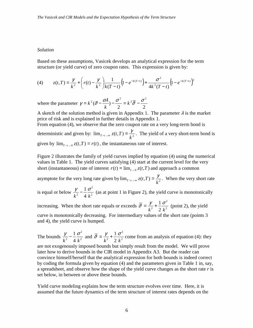
Solution Based on these assumptions, Vasicek develops an analytical expression for the term structure (or yield curve) of zero coupon rates. This expression is given by:
(4) ( ) ( )2)(3
2)(
22 1)(4
1)(
1)(),( tTktTk etTk
etTkk
trk
Ttz −−−− −−
+−−
−+= σγγ
where the parameter 22
)(2
22
2 σϑσσλϑγ −=−−= kk
k
A sketch of the solution method is given in Appendix 1. The parameter λ is the market price of risk and is explained in further details in Appendix 1. From equation (4), we observe that the zero coupon rate on a very long-term bond is
deterministic and given by: 2),(limk
TtztTγ=∞→− . The yield of a very short-term bond is
given by )(),(lim 0 trTtztT =→− , the instantaneous rate of interest. Figure 2 illustrates the family of yield curves implied by equation (4) using the numerical values in Table 1. The yield curves satisfying (4) start at the current level for the very short (instantaneous) rate of interest ),(lim)( 0 Ttztr →= τ and approach a common
asymptote for the very long rate given by 2),(limk
TtztTγ=∞→− . When the very short rate
is equal or below 2
2
2 41
kkσγ − (as at point 1 in Figure 2), the yield curve is monotonically
increasing. When the short rate equals or exceeds 2
2
2 21
kkσγϑ += (point 2), the yield
curve is monotonically decreasing. For intermediary values of the short rate (points 3 and 4), the yield curve is humped.
The bounds 2
2
2 41
kkσγ − and 2
2
2 21
kkσγϑ += come from an analysis of equation (4): they
are not exogenously imposed bounds but simply result from the model. We will prove later how to derive bounds in the CIR model in Appendix A3. But the reader can convince himself/herself that the analytical expression for both bounds is indeed correct by coding the formula given by equation (4) and the parameters given in Table 1 in, say, a spreadsheet, and observe how the shape of the yield curve changes as the short rate r is set below, in between or above these bounds. Yield curve modeling explains how the term structure evolves over time. Here, it is assumed that the future dynamics of the term structure of interest rates depends on the

The Vasicek and CIR Models and the Expectation Hypothesis of the Term Structure
evolution of the short rate of interest that follows a stochastic process given by (2). As time passes, shocks push the short rate below, in between, or above the bounds, generating a steepening, a flattening or an inversing of the curve.2 In conclusion, the Vasicek model implies that the shape of the yield curve essentially depends on the value of the short rate relative to some bounds. This explanation seems, a priori, quite different from the “classical” explanations of the yield curve based on expected future short rates and premium for risk. This, however, is not the case, as explained in the next section. In particular, we will show that equation (4) can be rewritten as:
( )( )Tt
tT
dxtIxrETtz
T
tx t,
)()((),( π+
−= ∫ =
In other words, the long rate is an average of expected short (instantaneous) rates plus a premium, as assumed by the biased expectation hypothesis.
2 One empirical fac
In the Vasicek mod
rate tends to revert 2, and that the term
4154.0 −−=λ p
sloping yield curve
z(t,T)
2
3
%4.1021
2
2
2 ==+ ϑσγkk
%49.82 =kγ = ),(lim TtztT ∞→−
Figure 2: yield curve modeling in Vasicek (1977)
),(lim)( 0 Ttztr tT →−=
4
7
t is that the yield curve is upward-sloping more o
el, we can show that if kσλ
43−
p , then ϑ p
to ϑ , this condition implies that we will often ob structure is upward sloping more often than it is
148.03 −=kσ
, and thus this specific calibratio
.
1
kγ
s
ften than downward-sloping.
2
2
2 41
kσ− . Recalling that the short
erve situations like point 1 in Figure downward sloping. In Table 1,
n should on average lead to an upward
%52.741
2
2
2 =−kkσγ
Term to maturity, T-t

The Vasicek and CIR Models and the Expectation Hypothesis of the Term Structure
Table 1: Parameters for the Vasicek model Parameters K 0.147 ϑ 0.074 σ 0.029 λ -0.154
κσλϑϑ −=
0.104
2)(
22 σϑγ −= k
0.001835
2kγ
0.08491
2
2
2 41
kkσγ −
0.07519
Source: Bolder (2001) 1.2 The forward rate and the expectations hypothesis of the term structure
The forward rate The yield curves in Figure 2 are the curves for the zero coupon rates. In order to obtain a better understanding of these curves, we can also introduce forward rates curves. The derivation of the zero coupon rates is sufficient for the determination of the forward rates. Indeed, we show in this subsection that forward and zero-coupon rates are related to each other as marginal and average cost curves in economics. Suppose the following time line: and deat timeat timearbitra
T1 T2
t8
fine z(t, Ti) as the zero coupon interest rate at time t for an investment that matures Ti, and F(t, Ti, T2) as the forward interest rate at time t for an investment that starts T1 and maturing at T2. Assuming continuous compounding and assuming away ge opportunities, the following condition must hold:

The Vasicek and CIR Models and the Expectation Hypothesis of the Term Structure
9
12
112221
))(,())(,,())(,(
))(,())(,(),,(
22122111
TTtTTtztTTtzTTtF
eee tTTtzTTTTtFtTTtz
−−−−=⇒
= −−−
Given the time line drawn above, we know that:
( ) ( )tTTTtT −+−=− 1122 which permits to rewrite the forward rate as:
(5) [ ] ( )( )12
112221 ),(),(),(),,(
TTtTTtzTtzTtzTTtF
−−−+=
Equation (5) illustrates the well-known relationship between a zero-coupon yield curve and the forward curve. If the zero coupon curve is flat, then the term in square bracket in equation (5) equals zero, and the forward rate is equal to the zero rate. For an upward- (downward-) sloping zero coupon curve the forward rate is higher (lower) than the zero rate. In parallel to the concept of an instantaneous interest rate, there exists an instantaneous forward rate. This is the forward rate that is applicable to a very short future time period that begins at time T. Taking limits as T2 approaches T1 in the equation above and letting the common value of the two be T, we obtain a series of equivalent expressions for the instantaneous forward rate:
(6)
( )
( )
( )
),(
),(
),(
(1))equation (by ),(ln),(
))(,(),(
),(),(),,(lim),( 2112
TtPdT
TtdP
Ttf
TtPdTdTtf
tTTtzdTdTtf
tTdT
TtdzTtzTTtfTtf TT
−=
−=
−=
−+== →
Integrating (6), obtains:

The Vasicek and CIR Models and the Expectation Hypothesis of the Term Structure
10
(7)
[ ] ]
tT
dxxtfTtz
tTTtzdxxtf
ttttztTTtztxxtzdxdx
txxtzddxxtf
T
tx
T
tx
T
tx
Tt
T
tx
−=
⇒
−=
−−−=−=−=
∫
∫
∫∫
=
=
==
),(),(
))(,(),(
))(,())(,())(,())(,(),(
Given the fact that )(),( trttf = , the instantaneous rate of interest, equation (7) can also be written as:
tT
dxxtftrz(t,T)
T
dttx
−
+= ∫ +=
),()(
Hence, the zero coupon rate is the average of the instantaneous forward rates with trade dates between time t and T. The zero coupon rate is the average cost of borrowing over a period (T-t), whereas the forward rate is the marginal cost of borrowing for an infinitely short period of time. The definition of the forward rate in (6) permits to compute the forward rate in the Vasicek model (see details in Appendix 1):
(8) ( ) )()()(2
2
2 )(12
),( tTktTktTk etreekk
Ttf −−−−−− +−
+= σγ
Given the one-to one relationship between the zero coupon and the forward curves, all we need to explain the shape of the zero coupon curve is to explain the shape of the forward curve. The Vasicek model and the expectation hypothesis of the term structure All term structure theories assume equation (7), that is, they all assume that the long rate is an average of forward rates over the life of the bond. This results from assuming that no profitable riskless arbitrage is possible. Where term structure theories differ is in whether they consider that forward interest rates are equal or not to expected future short interest rates. The diagram below shows a typology of term structures theories. Appendix 2 reviews these theories in detail. According to the pure (or unbiased) expectations hypothesis of the term structure, forward rates and expected short rates are driven to equality. If not, forward rates are considered to be a biased predictor of future short rates and their difference is the risk

The Vasicek and CIR Models and the Expectation Hypothesis of the Term Structure
11
premium. In this section we show that the Vasicek model is consistent with a biased expectation theory of the term structure.
A Typology of Term Structure Theories
Return-to-Maturity
Local Interpretation
Pure Expectations Theory
Liquidity Preference Theory
Preferred Habitat Theory
Biased Expectations Theory
Expectations Theory Market Segmentation Theory
Term Structure Theories
Figure 3 illustrates that in the Vasicek model, the forward rate is a biased predictor of the expected short rate. Using numerical values in Table 1, Panel a in Figure 3 illustrates that, according to the Vasicek model, if the current short rate r(t), is equal to
%52.741%4.7 2
2
2 =−=kkσγϑ p , as at point 1, the yield curve z(t,T) will be upward
sloping. Also, as shown in the previous subsection, an upward-sloping yield curve is associated with a forward rate curve f(t,T) that must be upward-sloping and above the zero coupon curve as shown in Figure 3. But we also know from the previous subsection that when the short rate is equal to ϑ, its long-term mean reverting value (as at point 1 in panel b), it is expected that future short rates remain at this level. This implies that the forward rate is not equal to the expected future short rate (ϑ in this particular case) or, in other words, that the forward rate is a biased predictor of future short rates and thus that the forward rate is equal to the expected future short rate plus a risk premium. Graphically, the premium for the particular case illustrated in Figure 3 is the vertical distance between the forward rate curve and the horizontal at ϑ. Analytically, the premium π(t,T), is defined as the difference between the forward rate and the expected short rate. (9) ),()()((),( TttITrETtf π+= where I(t) is the relevant information set at time t.

The Vasicek and CIR Models and the Expectation Hypothesis of the Term Structure
12
In the previous section we saw that the instantaneous forward rate and the expected future short rate are respectively given by equations (7) and (3) and restated here as:
( ) )()()(2
2
2 )(12
),( tTktTktTk etreekk
Ttf −−−−−− +−
+= σγ
and
( ) ( ) [ ] )()( )()1()( )()( )( tTktTk etretrTrEtITrE −−−− +−== ϑ
Hence, the term premium is given by:
(10) ( ))()(2
2
2 12
),( tTktTk eekk
Tt −−−− −
+−= σϑγπ
We can thus rewrite the forward rate as:
(11) ( ) ( )444444 3444444 21
444 3444 21
),(
)()(2
2
2ratespot future Expected
)( 12
)(),(
Tt
tTktTktTk eekk
etrTtf
π
σϑγϑϑ −−−−−− −
+−+−+=
Observe that:
2)( ),(limk
TtftTγ=∞→− and )(),(lim 0)( trTtftT =→− .
As well, ϑγπ −=∞→− 2)( ),(limk
TttT and 0),(lim 0)( =→− TttT π
These limits explain the way we have drawn the forward rate and the term premium in Figure 3.

The Vasicek and CIR Models and the Expectation Hypothesis of the Term Structure
%4.7))()(( ==ϑtrTrE
π(t,T)
z(t,T)
1
%49.82 =kγ
Figure 3: The forward rate as biased predictor
(Panel a)
%52.741
2
2
2 =−kkσγ
Term to maturity, T-t
(Panel b)
( ))()( trTrE( )
t
z(t,T)
f(t,T)
))()(( ))()(( 21 ϑϑ == trTrEtrTrEr(t)
),( Ttπ
1
13
T1 T2
ϑ = 7.4%
Time horizon

The Vasicek and CIR Models and the Expectation Hypothesis of the Term Structure
14
That the (instantaneous) forward rate is a biased predictor of the future (instantaneous) spot rate is often expressed in a different but analogous statement that the long rate is the average of future expected short rates over the life of the bond, plus a premium. Analytically, using (7) and (9), yields:
(12)
( )
( )
( )4434421444 3444 21Tt
T
tx
T
tx t
T
tx
T
tx
tT
dxxt
tT
dxtIxrETtz
tT
dxxttIxrE
tT
dxxtfTtz
, Premium,ratesshort expected future of Average
),()()((),(
),()()((),(),(
π
π
π
−+
−=
−
+=
−=
∫∫
∫∫
==
==
The expectation hypothesis, the liquidity theory and the preferred habitat theory all postulate the equation (12), with various specifications for the function ( )Tt,π . In the particular case of the Vasicek model, substituting equations (3) and (10) into (12), obtains: (13)
( )[ ] ( )tT
dxeekk
tT
dxetr
tT
dxxtfTtz
txkT
tx
txkT
tx
txkT
tx
−
−
+−
+−
−+=
−=
−−
=
−−
=
−−
=∫∫∫
)()(2
2
2)( 12)(),(
),(
σϑγϑϑ
As shown in Appendix 1, the solution of this integral is:
( ) ( ) ( )44444444444 344444444444 2144444 344444 21
),( Premium,
2)(3
2)(
2
2
ratesshort expected future of Average
)( 114
111))((1),(
Tt
tTktTktTk etTk
etT
kkk
etT
trk
Ttz
π
σγϑ
ϑγϑϑ −−−−−− −−
+−−
−
+
−+−
−−+=
After some simple manipulations, we can obtain equation (4), which confirms that the Vasicek model provides an analytical solution for the long rate that can be interpreted in the traditional framework of the biased expectations hypothesis. Note that by setting r(t) = ϑ (as it was assumed in Figure 3) in the equation above, we obtain that ),(),( TtTtz πϑ += . This explains why the premium ),( Ttπ in Figure 3 is drawn as the difference between z(t,T) and ϑ .3
3 As an application of the mean-value theorem, ( )Tt,π may be viewed as a distance, as drawn in Figure 3, or an average surface. In case of Figure 3, the average of expected future short rates over the horizon t --T is simply ϑ [This is the area in panel a under ϑ, between t and T, that is ϑ(T-t), divided by (T-t)] plus
( )Tt,π , which is the area described by the function π(t,T) = f(t,T)-ϑ divided by (T-t).

The Vasicek and CIR Models and the Expectation Hypothesis of the Term Structure
15
2. The Cox, Ingersoll and Ross “1 factor” model
Cox Ingersoll and Ross (1985) establish that when the very short interest rate is below the
long-term yield given by λγ
ϑττ ++=∞→ k
kz 2)(lim , the term structure is uniformly rising.
With an interest rate in excess of λ
ϑ+kk , the term structure is falling. For intermediate
values of the interest rate, the yield curve is humped. Hence, using the numerical values in Table 2 , CIR derive the shapes for yield curves given in Figure 4. The term to maturity is given by τ = T-t. It can be shown that the CIR model is a particular case of the affine model, whose properties for yield curves are given in Figure 5. Both the CIR model and its more general formulation, the affine model, are consistent with the biased expectation theory. Showing that this is the case is very similar to the derivations given for the Vasicek model, and we will not pursue this any further. However, we show in Appendix A3 how to derive the bounds given in Figure 4 and 5 for the CIR and affine models. Table 2: Parameters for the CIR model Parameters K 0.655 ϑ 0.073 σ 0.136 λ -0.313
22 2)( σλγ ++= k 0.392372
λγϑ++ k
k2
0.13022
λϑ+kk
0.13981
Source: Bolder (2001)

The Vasicek and CIR Models and the Expectation Hypothesis of the Term Structure
16
1
z(τ)
3
2
1
Figure 4: Yield curve modeling in CIR (1985)
τ = 0 τ→
)(lim)( 0 ττ ztr →=
z(τ)
3
2
Figure 5: The affine m
)(lim)( 0 ττ ztr →=
τ = 0 τ→
%981.13=+ λϑ
kk
∝
−
l
ode
∝
%022.132)(lim =++
=∞→ λγϑττ k
kz
Term to maturity, τ
ϑ =7.3%
l
0
120
01
0
1
0
0 222 β
ββ
αββα
αβ
−
−
( )( )2
0200
102001
2
)2(2)(im
βαα
ββαααττ
++−
−++−=∞→ z
Term to maturity, τ

The Vasicek and CIR Models and the Expectation Hypothesis of the Term Structure
17
3. Conclusion Best practises of debt management require the use of modern theories of the term structure based on the seminal papers by Vasicek (1977) and Cox, Ingersoll and Ross (1985). These models have been used to analyse the issue of public debt management both at the Bank of Canada [Bolder (2002)], and at the Department of Finance [Debt Management Strategy 2003-2004], and in other countries [e.g., Danish Nationalbank (2001)]. An objective of this paper is, first, to “demystify” these models to the non-experts of the field by showing that they “simply” belong to the class of interest rate term structures with biased expectations hypothesis. Thus, these models generate yield curves where the long interest rate is an average of future expected short rates plus a term premium. In these models, the expected future short rates are consistent with an exogenously specified process for the short rate. Secondly, this paper documents the Vasicek and CIR term structure of the interest rates that will be introduced into a macro-economic stochastic simulation model (SSM) developed at the Department of Finance. The final aim will be to use the SSM with alternative term structures of interest rates to gauge the robustness of our earlier results described in Georges (2003), which suggests that a shorter debt maturity structure is less expensive on average and also less risky from the point of view of the overall budget balance if demand shocks prevail over the business cycle. One key issue, however, in introducing the Vasicek or CIR term structures into a macro-economic simulation model is to reconcile the assumed exogenously given process for the short interest rate with the typical macro view of a Central Bank’s monetary policy rule that sets short term interest rates to offset deviations of expected inflation rate from its target. There are alternative ways to think of this issue and this should be considered in future research. A well-known shortcoming of the (multi-factors) affine term structure models [e.g., the Vasicek and CIR models and their extensions (Duffie and Kan (1996)] is that they cannot help us understand the mechanism through which the macro-economy influences the term structure. Describing the joint behavior of the yield curve and macroeconomic variables is, however, important for bond pricing, investment decision and public policy. Macro- and financial economists have argued that the term structure is intimately linked to macro-variables. For example, Fama (1986) asserts that term premiums tends to increase with maturity during good times, but humps and inversions in the term structure are common during recessions. Bernanke and Blinder (1992), Estrella and Hardouvelis (1991), and Mishkin (1980) explore the potential of using the spread between long-term and short-term yields as an indicator of monetary policy, future economic activity, and future inflation. We thus plan to examine in future research a new literature that provides a macroeconomic interpretation for the affine term structure models [e.g., Ang and Piazzesi (2001), Dewachter and Lyrio (2003), Wu (2001)].

The Vasicek and CIR Models and the Expectation Hypothesis of the Term Structure
18
APPENDIXES
A1. The Vasicek model
Computing the zero coupon rate in the Vasicek model We start with the process for the short-term (instantaneous) interest rate, r(t). Vasicek assumes that it follows an Ornstein-Uhlenbeck process: (1) dWdtrktdr σϑ +−= )()( The instantaneous drift )( rk −ϑ represents a force that keeps pulling the short rate towards its long-term mean ϑ with a speed k proportional to the deviation of the process from the mean. The stochastic element, which has a constant instantaneous variance σ 2, causes the process to fluctuate around the level ϑ in an erratic, but continuous, fashion. dW is a standard Wiener process. Vasicek assumes that a market exists for bonds of every maturity. We denote the value of a default-free pure discount bond as the function P(t,T,r(t)). The first argument, t, refers to the current time, while the second argument, T, represents the bond maturity date. Vasicek also assumes that the price of the bond is a function of the short rate. Applying Itô’s lemma, and using (1) obtains:
(2) [ ]
dWPdtrkPPP
dtPdWdtrkPdtP
dtPdrPdtPtrTtdP
rrrrt
rrrt
rrrt
σϑσ
σσϑ
σ
+
−++=
++−+=
++=
)(21
21)(
21))(,,(
2
2
2
This is a stochastic differential equation. The important contribution of Vasicek is to transform this into a differential equation that does not depend on the Wiener process. He thus builds a portfolio of bonds with different maturities whose shares are chosen to make it risk-free. Instead of going through the steps of the original paper, we simply do the following observations. Box 1 describes a more “orthodox” route. Dividing by P(t,T,r(t)), obtains the rate of return of the bond:
(3) {
dWPP
dtP
rkPPP
trTtPtrTtdP
pdppdp
rrrrt
//
)(21
))(,,())(,,(
2
σµ
σϑσ
+
−++
=44444 344444 21

The Vasicek and CIR Models and the Expectation Hypothesis of the Term Structure
19
pdp /µ and pdp /σ are the mean and standard deviation of the instantaneous rate of return at time t on a bond with maturity date T, given that the current spot rate is r(t) = r. If the bond is risk free in the sense that the interest rate is constant (non-stochastic), its return over the interval dt is4:
rdtrTtPrTtdP =),,(),,(
However, given the process in (1), the bond is not risk free because the future value of the short rate is stochastic. Vasicek shows that in this case the return on a bond is given by:
(4) [ ]
[ ]dtdWPPdttr
rTtPrTtdP
dtdWdttrrTtPrTtdP
r
pdp
λσ
λσ
+=−
+=−
)(),,(),,(
)(),,(),,(
/
Note that if σ = 0 in (1) (and thus in (4)), the interest rate would be non-stochastic and the bond’s return over the short interval of time dt would equal r(t)dt, the risk free return. The right-hand side of (4) contains two terms: a deterministic term in dt and a random term in dW. The presence of the Wiener increments dW shows that this is not a risk-free bond. The deterministic term may be interpreted as the excess return above the risk-free rate for accepting a certain level of risk. In return for taking the extra risk the bond return makes an extra λdt per unit of extra risk, dW. The parameter λ is therefore called the market price of risk. Using (3) and (4), obtains:
dWPPdt
P
rkPPPdW
PPdt
PPtr
trTtPtrTtdP r
rrrtrr σ
ϑσσλσ +
−++
=+
+=
)(21
)())(,,())(,,(
2
4 This simply means that an amount of money P(t) at time t will grow up to ))(,(
111)()( tTTtzetPTP −= over
the period (T1-t), where z(t,T1) is a continuously compounded p.a. interest rate. This implies that:
)(1)()(ln)(),(lim
))(ln()(ln(),(
10
1
11
1 tPdttdP
dttPdtrTtz
tTtPTPTtz
tT ===⇒
−−=⇒
→−

The Vasicek and CIR Models and the Expectation Hypothesis of the Term Structure
20
Box 1. Transforming equation (2) into a differential equation that does not depend on the Wiener process. Let us construct a portfolio, denoted V, of two discount bounds that pay 1 unit of currency when they mature at time T1 and T2 and with current prices P1(t, T1) and P2(t,T2). The weights of each bond in the portfolio are u1 and u2. The return of this portfolio over the interval of time dt is given by:
(B1) ),(),(
),(),()(
22
222
11
111 TtP
TtdPuTtPTtdPu
dttdV +=
Substituting equation (2) into (B1), obtains:
+
−++
+
+
−++
=
dWTtP
Pdt
TtP
rkPPPudW
TtPP
dtTtP
rkPPPu
dttdV
PdPPdPPdPPdP
rrrrt
rrrrt
4342144444 344444 214342144444 344444 212/22/21/11/1
),(),(
)(21
),(),(
)(21
)(
22
,2
22
,22
,2,2
211
,1
11
,12
,1,1
1
σµσµ
σϑσσϑσ
(B2) dWuudtuu
dWudtudWudtudt
tdV
PdPPdPPdPPdP
PdPPdPPdPPdP
)()(
)(
2/221/112/221/11
2/222/221/111/11
σσµµ
σµσµ
+++=
+++=
The key is to build the portfolio V such that it is riskless, and thus independent of the dW term. We thus need to pick the weights u1 and u2 such that:
=+=+
10
21
2/221/11
uuuu PdPPdP σσ
This requires choosing:
−=
−−=
2/21/1
1/12
2/21/1
2/21
PdPPdP
PdP
PdPPdP
PdP
u
u
σσσ
σσσ
Substituting these values for u1 and u2 in (B2) obtains:
3210
2/22/21/1
1/11/1
2/21/1
2/2 )0()(
=
+
−
+−
−= dWdtdt
tdVPdP
PdPPdP
PdPPdP
PdPPdP
PdP µσσ
σµσσ
σ

The Vasicek and CIR Models and the Expectation Hypothesis of the Term Structure
21
Because this portfolio is risk free over the interval of time dt, it should earn the risk free instantaneous rate: r(t)dt. This implies that:
(B3)
443442144 344212/22/2 )(
1/1
1/1
)(
2/2
2/2
2/22/21/1
1/11/1
2/21/1
2/2
)()(
)(
PdPPdP t
PdP
PdP
t
PdP
PdP
PdPPdPPdP
PdPPdP
PdPPdP
PdP
trtr
tr
λλ
σµ
σµ
µσσ
σµσσ
σ
−=−⇒
=
−
+−
−
We note that (B3) holds for any arbitrary maturity T1 and T2. Thus the ratio in (B3) must be independent of the maturity of the bond, that is, constant across all maturities. Let λ(t) denote the common value of such a ratio for a bond of any maturity date:
(B4) PdP
PdP trt
/
/ )()(
σµλ −
=
The quantity λ(t) is called the market price of risk, as it specifies the excess return on a bond over the risk-free rate per quantity of risk. Substituting equation (3) into (B4), obtains:
(B5)
( ) 0)(2
)()(
)()(
21
)(
2
2
=−+−−+
⇒
−
−++
=
PtrPPtrkP
trP
rkPPP
PPt
rrrt
rrrtr
σσλϑ
ϑσσλ
which is equation (5) of Appendix 1.

The Vasicek and CIR Models and the Expectation Hypothesis of the Term Structure
22
(5) ( ) 0)()(21 2 =−−−++ PtrrkPPP rrrt σλϑσ
Hence, the stochastic differential equation (2) has been transformed into a partial differential equation that is independent of the Wiener process. Before solving the differential equation, it is interesting to note the following by rewriting (5) as:
)()(
21
//
2
trP
PP
rkPPP
pdppdp
rrrrt
=−−++
3214444 34444 21λσµ
σλϑσ
Hence, this differential equation simply means that the price of the bond P(t,T,r(t)), must be such that, for all holding periods, the expected excess return of the bond over the risk-free rate of interest is the market price of risk of r, (λ), multiplied by the quantity of r-risk present in P, ( pdp /σ ):
pdppdp tr // )( λσµ =− On the right-hand side of the equation, we are, therefore, multiplying the quantity of r-risk by the price of r-risk. The left-hand side is the expected return in excess of the risk-free interest rate that is required to compensate for this risk. This equation is analogous to the capital asset pricing model, which relates the expected excess return on a stock to its risk. We are now ready to solve the differential equation (5). For this, we will assume that the price function has the following shape: (6) rBArTtBTtA erPerTtP )()(),(),( ),(),,( τττ −− === where tT −=τ is the term to maturity. This change of variable is introduced for simplicity. The partial derivatives are as follows:
(7) ( )
)()()()(
)())(')('
2 ττττ
τττ
PBPPBP
PrBAP
rr
r
t
=
−=+−=
Substituting these values into (5), obtains:
( ) ( ) 0)()('1)(2
)()(' 22
=−−−+−−− τττστσλϑτ kBBrBBkA
This can hold only if:
The Vasicek and CIR Models and the Expectation Hypothesis of the Term Structure
23
(8) 1)()(' =+ ττ kBB and:
(9) ( ) 0)(2
)()(' 22
=+−−− τστσλϑτ BBkA
The boundary conditions are given by the fact that a bond has a terminal value (when τ=0) of P(T,T)=P(0) =1, such that, given (6):
0)0()0(1)0( )0()0(
==⇒== −
BAeP rBA
The solution of the differential equations (8) and (9) are respectively:
(10) )1(1)( ττ kek
B −−=
(11) k
Bk
BA4
)())(()(22
2
τσττγτ −−=
where:
22)(
22
22 σϑσσλϑγ −=−−= k
kk
Given that the zero coupon rate of interest is defined as:
(12) )()(ln),(ln),( ττ
τ zPtT
TtPTtz =−=−
−=
finally obtains:
( ) ( )
( ) ( )2)(3
2)(
22
2
3
2
22
1)(4
1)(
1),(),(),(
or
14
11)()()(
tTktTk
kk
etTk
etTkk
rktT
rTtBTtATtz
ek
ekk
rk
rBAz
−−−−
−−
−−
+−−
−+=
−+−=
−+−
−+=+−=
σγγ
τσ
τγγ
ττττ ττ
Computing the forward rate First, let us note the following results based on equations (10) and (11):

The Vasicek and CIR Models and the Expectation Hypothesis of the Term Structure
24
( )( )
( )
( ) ( )( )
( ) ( )( ))()(2
)(2
)()(2
'2
2)(2
2
)(
22
2
)(
124
1),(),('
12),(),(
11),(
),(),('
4),()(),(),(
11),(
tTktTktTk
tTktTk
tTk
tTk
tTk
eekk
ekdT
TtdATtA
eekdT
TtdBTtB
ek
TtB
edT
TtdBTtB
kTtB
ktTTtBTtA
ek
TtB
−−−−−−
−−−−
−−
−−
−−
−−−==
−==
−=
==
−−−=
−=
σγ
σγ
Using (6), and the definition of the forward rate given in the text (equation (6)), we can thus derive the forward rate in the Vasicek model.
( )⇒
−=
⇒= −
),(),('),('),(
),( ),(),(
TtPrTtBTtAdT
TtdP
eTtP rTtBTtA
)(),('),('),(
),(
),( trTtBTtATtP
dTTtdP
Ttf +−=−=
Substituting the results derived above for A’ and B’, yields:
(13) ( ) ( )( )
( ) )()()(2
2
2
)()()(2
2)(
2
)(12
),(
)(12
1),(
tTktTktTk
tTktTktTktTk
etreekk
Ttf
treeek
ek
Ttf
−−−−−−
−−−−−−−−
+−
+=
+−+−=
σγ
σγ
Vasicek and the expectations hypothesis From equations (10) and (12) in the body of the text, the term premium is:
( )
∫∫∫∫
∫
∫
=
−−
=
−−
=
−−
=
−−
=
−−
=
−
+
−−
−=
−
+−=
=−
T
tx
txkT
tx
txkT
tx
txkT
tx
txkT
tx
txk
T
tx
dxek
dxek
dxek
dxk
dxeekk
dxxttTTt
)(22
2)(
2
2)(
22
)()(2
2
2
22
12
),())(,(
σσϑγϑγ
σϑγ
ππ

The Vasicek and CIR Models and the Expectation Hypothesis of the Term Structure
25
( ) ( ) ( )
( )
( ) ( )2)(3
2)(
22
)(23
2)(
3
2
3
2
3
2)(
22
)(23
2)(
3
2)(
22
3
2)(2
3
2
2
2)(
2
2
2)(
22
)(22
2)(
2
2)(
22
14
11)(
424211)(
14
12
11)(
441
21
211)(
21
21
21))(,(
tTktTk
tTktTktTk
tTktTktTk
tTktTktTk
T
t
txkT
t
txkT
t
txkT
t
ek
ekk
tTk
ek
ekkk
ekk
tTk
ek
ek
ekk
tTk
ke
kkke
kkkke
kktT
k
ekk
ekk
ekk
xk
tTTt
−−−−
−−−−−−
−−−−−−
−−−−−−
−−−−−−
−+−
−+−
−=
+−−+−
−+−
−=
−−−+−
−+−
−=
−++−
−+
−−−
−=
+−
−−
−=−
σγϑϑγ
σσσσγϑϑγ
σσγϑϑγ
σσσσγϑγϑϑγ
σσγϑϑγπ
From equations (3) and (12) in the body of the text the expectation term is given by:
( ) ( )[ ]
( ))(
)(
)(
11)(
1)(
)()()((
tTk
T
t
txkT
t
T
tx
txkT
tx t
ektT
tr
ektT
trtT
xtT
dxetr
tT
dxtIxrE
−−
−−
=
−−
=
−−−+=
−−−
−=
−
−+=
−∫∫
ϑϑ
ϑϑ
ϑϑ
Combining the expectations term and the premium derived above, yields:
( ) ( ) ( )44444444444 344444444444 2144444 344444 21
π
σγϑ
ϑγϑϑ
Premium,
2)(3
2)(
2
2
ratesshort expected future of average
)( 114
111))((1),( tTktTktTk etTk
etT
kkk
etT
trk
Ttz −−−−−− −−
+−−
−
+
−+−
−−+=
The local version of the expectations hypothesis In the previous section of this appendix, we assumed that the expectations hypothesis meant that forward rates and expected spot rates are driven to equality; any deviation is the term premium. There are, however, alternate forms or interpretations of the expectations hypothesis, as described by Cox, Ingersoll, and Ross (1981) and described also in Appendix A2. According to the “local” version of the expectations hypothesis, expected holding period returns of bonds of different maturities (of different T, but for same t) must be equalized for one specific holding period. The natural choice of holding period is the next basic (i.e., “shortest”) interval, dt. In other words, this means that:
The Vasicek and CIR Models and the Expectation Hypothesis of the Term Structure
26
[ ])(),(
),(
trdt
TtPTtdPE
= (for all T)
In this interpretation, the risk premium is thus identified as:
[ ])(),(
),(
),( trdt
TtPTtdPE
Ttl −=π
We can use the results of this appendix to obtain the premium in the Vasicek model implied by the local version of the Expectations Hypothesis. Using (3) and (4), and recalling that the increments of a Wiener process are normally distributed with E(dW) =0 and Var(dW) = dt, yields:
[ ] dtPPdttrdt
TtPTtdPE r
pdp λσµ +== )(),(
),(/
[ ]
λσµPPtr
dtTtP
TtdPEr
pdp +== )(),(),(
/
and thus:
(14)
[ ]λσπ
PPtr
dtTtP
TtdPE
Tt rl =−= )(),(),(
),(
In the Vasicek model, we can compute the risk premium as follows, substituting equations (7) and (10) into (14):
[ ]( ))(11),()(),(
),(
),( tTkl ek
TtBtrdt
TtPTtdPE
Tt −−−−=−=−= σλλσπ
Note: limit of premium when T-t→∝ is k1σλ− , which, by definition, is ϑϑ − .
We are now left with two versions of deviations from the pure expectations hypothesis. According to the deviation from the return-to-maturity interpretation, the term premium is:
( ))()(2
2
2 12
),( tTktTk eekk
Tt −−−− −
+−= σϑγπ

The Vasicek and CIR Models and the Expectation Hypothesis of the Term Structure
27
Recalling the definition 22
)(2
22
2 σϑσσλϑγ −=−−= kk
k , yields:
(15)
( )
( )2)(2
2
)()(2
2
2
2
12
),(),(
122
),(
tTkl
tTktTk
ek
TtTt
eekkk
Tt
−−
−−−−
−−=
⇒
−
+−−=
σππ
σσσλπ
where ),( Ttlπ is the term premium when deviations from the local interpretation of the pure expectation hypothesis are considered.

The Vasicek and CIR Models and the Expectation Hypothesis of the Term Structure
28
A2. A typology of the theories of the term structure of interest rates All theories of the term structure of interest rates assume away riskless arbitrage opportunities arising from differences between current forward and spot rates. This implies equation (7) in the body of the text, rewritten here as:
(16) tT
dxxtfTtz
T
tx
−= ∫ =
),(),(
Furthermore, pure and biased expectations theories of the term structure of interest rates also assume that investors and borrowers are willing to shift from one maturity sector to another to take advantage of opportunities arising from differences between expectations of future spot rates and current forward rates. Thus, a key assumption is that bonds of different maturities are (to a certain extent) substitutable. Another theory, the segmented market theory sees markets for different-maturity bonds as completely separate and segmented. Bonds of different maturities are not substitutable. The interest rate for each bond with a different maturity is then determined by the supply and demand for that bond with no effects from expected returns on other bonds with other maturity. In the following we focus exclusively on pure and biased expectations theories. Pure expectations theory According to the pure expectation theory, the forward rate is equal to the expected interest rate, that is: )),((),,( 2121 TTzETTtF t= . This also holds for an arbitrarily short period, when T2→T1 and thus, using instantaneous forward and spot rates, yields: (17) ))()((),( tITrETtf = Substituting (17) into (16), results in:
(18) ( )
tT
dxtIxrETtz
T
tx
−= ∫ =
)()(),(
In other words, the interest rate on a long-term bond will equal an average of short-term interest rates that people expect to occur over the life of the long-term bond. For example, if people expect that short-term interest rates, r(x), will be 10 percent on average over the coming five years, the expectations hypothesis predicts that the interest rate on bonds with five years to maturity will also be 10 percent. If short-term interest rates were expected to rise even higher after this five-year period such that the average short-term interest rate over the coming 10 years is 11 percent, then the interest rate on a 10-year bonds would equal 11 percent and would be higher than the interest rate on a 5-year bond. Hence, under this view, a rising term structure for the long rates must indicate that the market expects short-term rates to rise throughout the relevant future period (in

The Vasicek and CIR Models and the Expectation Hypothesis of the Term Structure
the example, between year 5 and year 10). Similarly, a flat term structure reflects an expectation that future short-term rates will be generally constant, while a falling term structure must reflect an expectation that future short-terms rates will decline. A graphical representation which supposes that the short rate follows a mean-reverting process is particularly useful to improve our understanding of the pure expectation hypothesis.
Figure 6 Figure 6 above illustrates that toBecause the short rate is assumewill eventually increases to its lo
))()(( trTrE . This path represenany future time T conditional onT1) and z(t, T2) are determined, assessment, at time t, of the segmz(t, T1) is the average expected vexpected value of {r(x), t ≤ x ≤ Tthat an upward-sloping yield curexpectations hypothesis, reflectsrelevant time segment. The pure expectation theory is aobserve that interest rates on bonThe figure above illustrates this.mean reverting value, ϑ, such thwell. Because short rates are eximplies a flat yield curve with z(the short rate to r(t) at point 1. H
ϑ
Time horizon, x T1 T2
( )tT
dxtrxrETtz
T
tx
−= ∫ =
11
1 )()(),(
( )tT
dxtrxrETtz
T
tx
−= ∫ =
22
2 )()(),(
))()(( trTrE
1 r(t)
t
29
day, at time t, the short rd here to follow a mean-ng-term mean reverting ts the expected value of
the actual value of the saccording to the expecta
ents {r(x), t ≤ x ≤ T1}analue of {r(x), t ≤ x ≤ T1}2}, as drawn in Figure 6ve [z(t, T2)> z(t, T1)>r(t) the fact that short rates a
ble to explain some empds with different maturi
Suppose that the short-at future short rates are epected to remain constant, T1) = z(t, T2) = ϑ . Neistorically, short-term ra
ate is equal to r(t), (point 1). reverting process, the short rate value of ϑ along the path the short (instantaneous) rate for hort rate, r(t). The long rates z(t, tions hypothesis, by the d{r(x), t ≤ x ≤ T2}. In particular, and z(t, T2) is the average . This Figure clearly illustrates ], according to the pure re expected to increase over the
irical facts. For example, we ties move together over time. rate is initially at its long-term xpected to remain at this level as t over the time horizon, this xt suppose that a shock pushes tes have had the characteristic
The Vasicek and CIR Models and the Expectation Hypothesis of the Term Structure
30
that if they decrease today, they will then tend to be lower in the future than otherwise. Hence a decrease in short-term rates will lower people’s expectations of future short-term rates. This is illustrated in Figure 6 by the shift of the expectation schedule from the horizontal line in ϑ to the upward-sloping schedule, ))()(( trTrE . Given that long-term rates are the average of expected future short-term rates, a decrease in current and future expected short-term rates will also decrease long-term rates, (to their value shown in the graph, z(t, T1) < z(t, T2) < ϑ ). This causes short- and long-term rates to move together. A second empirical fact, which is well explained by the pure expectation hypothesis, is that when short-term rates are low, yield curves are more likely to have an upward slope and when short-term rates are high, yield curves are more likely to slope downward. This is again well illustrated by Figure 6. When short-term rates are low, (say at point 1) people generally expect them to rise to some normal level (ϑ) in the future, and the average of future expected short-term rates is high relative to the current short-term. Therefore long-term interest rates z(t, T1) , z(t, T2), etc., will be above current short-term rates and the yield curve would then have an upward slope. Unfortunately, the pure expectations hypothesis cannot explain the empirical fact that yield curves usually slope upward. A typical upward slope implies under this hypothesis that short-term interest rates are typically expected to raise in the future (as is shown in Figure 6). In practice, short-term interest rates are as likely to fall as they are to rise, and so the expectations hypothesis suggests that the typical yield curve should be flat rather than upward-sloping. As will be shown below, the biased expectation hypothesis can explain why a typical yield curve would be upward-sloping. Before doing this, we should however mention some interpretations of the pure expectation theory and highlight some inconsistencies initially considered by Cox Ingersoll and Ross (1981). We saw that if equation (17) and thus (18) held, then the interest rate on a long-term bond would equal an average of short-term interest rates that people expect to occur over the life of the long-term bond. However, we did not explain why equations (17) or (18) would hold. There are several interpretations of the pure expectation hypothesis. We will only mention two of them, the return-to-maturity and the local interpretations. First, let us rewrite equation (18) in terms of return:
(19) ( )[ ]∫− ====T
tx dxtIxrtTTtz eEeTtPTtP
TTP )()())(,(
),(1
),(),(
A first interpretation of the pure expected hypothesis, referred to as the return-to-maturity, suggests that the return that an investor will realize by rolling over short-term bonds over some investment horizon will be the same as holding a zero-coupon bond with a maturity which has the same investment horizon. Assuming continuous compounding but a discrete-time notation, the return-to-maturity suggests that:

The Vasicek and CIR Models and the Expectation Hypothesis of the Term Structure
31
(20)
[ ][ ]
∑=
=
⋅⋅⋅⋅=
−
=
+
−+⋅⋅⋅+++++
−+++−
1)1,(
),1()2,1()1,(
),1()2,1()1,())(,(
T
txxxz
t
TTzttzttzt
TTzttzttzt
tTTtz
eE
eEeeeEe
Switching to our continuous-time notation such that the one-period rate of interest z(x, x+1) becomes the instantaneous rate of interest r(x), we eventually obtain equation (19). Hence the return-to-maturity interpretation “rationalizes”, or justifies the statements given earlier in equation (19) and thus in equations (18) and (17). This does not, however, imply that these statements are correct. For the problems associated with these statements, see the next subsection. A second interpretation of the pure expectation theory, referred to as the local expectations form of the pure expectations theory, suggests that the expected holding period rate of return of bonds of different maturities must be equalized for one specific holding period. The natural choice of holding period is the next basic (i.e., “shortest”) interval. In other words, this means that:
[ ]
)(),(),(
trdt
TtPTtdPE
= (for all T)
Integrating the expression above (abstracting initially from the expectation operator), obtains:
∫∫ ===
T
tx
T
txdxxrdx
dxTxPTxdP
)(),(),(
Recalling that: dxTxP
TxdPTxP
dxTxdP
dxTxPd 1
),(),(
),(
),(),(ln == , obtains:
∫∫
=
=
−=
=−=−=−=T
tx
T
tx
T
t
dxxrTtP
dxxrTtPTtPTtPTTPTxP
)(),(ln
)(),(ln),(ln)1ln(),(ln),(ln),(ln
Taking the exponential and then the expectation operator (at time t), on both sides of the equation, recalling that at time t, P(t,T) is known (not random), successively yields:
∫= =
−T
txtIdxxr
eTtP)()(
),(

The Vasicek and CIR Models and the Expectation Hypothesis of the Term Structure
32
(21) ( )
( )∫−−
∫−
=
=
===
=
Ttx
Ttx
tIdxxrtTTtz
tIdxxr
eEe
TtPTtPTTP
eETtP
)()())(,(
)()(
1),(
1),(),(
),(
Now, it is tempting to shift the denominator to the nominator by getting rid of the minus sign in front of the integral and obtain equation (19). The local version of the expectation hypothesis would then fully rationalize the pure expectation hypothesis, and justify statements given earlier in equations (18) and (17). Strictly speaking, however, as noted by CIR (1981), this is incorrect because of Jensen’s inequality. To see this, set the random variable ∫− ===
Ttx trdxxry eex )()(~~ . Statement (19) would then lead to:
(19’) [ ]
=
== −−
xE
eEeEe y
ytTTtz~11
~~))(,( ,
whereas the statement in (21) leads to:
(21’) [ ] [ ]xEeEe y
tTTtz~
11~
))(,( ==− .
However, by Jensen’s inequality we know that if [ ]xEe tTTtz
~1))(,( =− , then
))(,(~1 tTTtzex
E −
f . We can illustrate this with an example. If a random variable x~ can
take on two values say, 0.90 and 0.92, with same probability, then
[ ] 91.02
92.090.0~ =+=xE and [ ] 0989.1~1))(,( ==−
xEe tTTtz . However,
0989.10990.12
92.01
90.01
~1
f=+
=
xE
Hence, strictly speaking, the local version of the expectation hypothesis cannot entirely “rationalize”, or justify the statements given earlier in equation (19) and thus in equations (18) and (17). However, that these statements can be exactly interpreted in terms of return-to-maturity, or only approximately interpreted in terms of the local form of the pure expectations hypothesis, does not imply that the first interpretation is more valid, in general than the second. Indeed, what really matters is whether the statements themselves [equations (17), (18), or (19)] are valid. For one thing, the left side of these equations is a rate (the forward or the long rate), or a return, that is known with certainty, and this is compared to an uncertain rate or return that depends on the random future short rate. To bring these two concepts into equality implies that it is assumed that agents are risk-neutral, and thus indifferent between a certain amount and the expected value of a random variable. Risk-averse agents, however, may require compensation for the risk involved when acting on the basis of an estimate of the average of short-term interest rates that they expect to occur over the life of the long-term bond. The next subsection

The Vasicek and CIR Models and the Expectation Hypothesis of the Term Structure
33
examines two types of risk involved in this context. After this, we will review the biased expectation hypothesis that compensates risk-averse agents with a risk premium. Drawbacks of the pure expectations theory The pure expectations theory neglects the two types of risk inherent in investing in bonds. The first, the reinvestment risk involves the uncertainty about the rate at which the proceeds from a bond that matures prior to the end of the investment horizon can be reinvested. For example, an investor who plans to invest for five years may invest in a five-year bond and hold it for five years, or invest in a 1-year bond and, when it matures, reinvest the proceeds in 1-year bonds over the entire five-year horizon. The risk in the second alternative is that the return over the five-year investment horizon is unknown because rates at which the proceeds can be reinvested until the end of the investment horizon are unknown. Hence, the return-to-maturity interpretation of the pure expectation theory, which suggests that the return that an investor will realize by rolling over short-term bonds will be the same as holding a long maturity bond over the same investment horizon, neglects the reinvestment risk. The second is the price or interest risk. For example, an investor who plans to invest for five years might invest in a five-year bond and hold it for five years, or invest, say, in a 10-year bond and sell it at the end of five-year. The return of the first strategy is known with certainty because the holding period coincides with the term to maturity of the bond. The investor knows the price of the bond when he buys it (say, $99.2) and he knows with certainty the price of the bond when he sells it because the bond matures and pays the promised nominal value (say, $100), which, by arbitrage must be the selling price. The return of the second strategy is unknown because the investor does not know the price of the bond when he will sell it five years from now. Hence, the local expectations form of the pure expectations theory, which suggests that the expected holding period returns of bonds of different maturities must be equalized for one specific holding period, neglects this type of risk. Biased expectations theories As said above, risk-averse agents require a compensation for taking risk. The biased expectation hypothesis recognise this by amending equation (17) as follows: (22) ),())()((),( TttITrETtf π+= where π(t,T) is a positive risk premium. Substituting (22) into (16), obtains:
(23) ( )
tT
dxTttIxrETtz
T
tx
−
+= ∫ =
),()()(),(
π
The Vasicek and CIR Models and the Expectation Hypothesis of the Term Structure
34
This leads to a situation where forward rates are greater than expected future spot rates, or long rates are greater than the estimation of the average of future short rates. Statements in equations (22) and (23) are usually rationalized with two forms or interpretations of the biased expectations hypothesis: the liquidity preference theory and the preferred habitat theory. The liquidity preference theory starts with the observation that, ceteris paribus, investors wish to deposit their money for short terms while borrowers wish to borrow at fixed rates for long terms. If the interest rates offered by financial intermediaries were such that that forward rates equalled expected future spot rates, long term rates would equal the average of expected future short-term rates. Investors would tend choose to deposit their funds for short terms and borrowers would tend to borrow for long terms simply because they would have no incentives to do otherwise given their preferences. Financial intermediaries would then find themselves financing substantial amounts of long-term fixed rates loans with short-term deposits. This would involve excessive interest-rate risk. In practise, in order to match depositors with borrowers and avoid interest-rate risk, financial intermediaries raise long-term rates relative to expected future short-term rates. This reduces the demand for long-term fixed-rate borrowing and encourages investors to deposit their funds for long terms. It also leads to a situation where forward rates are greater than expected future spot rates. In other words, the forward rate embodies a liquidity premium. The preferred habitat theory states that the interest rate on a long-term bond will equal an average of short-term interest rates expected to occur over the life of the long-term bond plus a term premium that responds to supply and demand conditions for that bond. The preferred habitat theory’s key assumption is that bonds of different maturities are substitutes, which means that the expected return on a bond does influence the expected return on a bond of a different maturity, but it allows investors to prefer one bond maturity over another. In other words, bonds of different maturities are assumed to be substitutes but not perfect substitutes. If investors prefer the habitat of short-term bonds over longer-term bonds, they might be willing to hold short-term bonds even though they have a lower expected return. This means that investors would have to be paid a positive term premium in order to be willing to hold a long-term bond. The preferred habitat and liquidity premium theories explain the empirical fact that yield curves typically slope upward by recognizing that the term premium rises with a bond’s maturity because of investors’ preferences for short-term bonds. Even if short term interest rates are expected to stay the same on average in the future, long-term interest rates will be above short-term interest rates, and yield curves will typically slope upward. Figure 7 illustrates this. When the short rate at time t is equal to its long-term mean reverting value ϑ, as at point 1, short interest rates are expected to stay unchanged but the long rate, z(t,T) 1 , is greater than their average value of ϑ by a premium π(t,T), leading to an upward-sloping yield curve [z(t,T) 1 > r(t)].

The Vasicek and CIR Models and the Expectation Hypothesis of the Term Structure
z(t,T) 2
How can the preferred habitat and liquidity premium theories explain the occasional appearance of inverted yield curves if the term premium is positive? It must be that at times short rates are expected to fall so much in the future that the average of the expected short-term rates is well below the current short-term rate. Figure 7 also explains this. If the short rate is at point 2 at time t, expected future short rates are expected to fall, and their average over the time horizon t—T is given by ( )
tT
dxtrxrET
tx
−∫ =
)()( . Even when the
positive term premium is added to this average, the resulting long-term rate z(t,T) 2 is below the current short-term interest rate r(t), leading to a downward-sloping yield curve [r(t) > z(t,T) 2].
2
Figure 7
35
z(t,T) 1
1
π(t,T)
π(t,T) ( )tT
dxtrxrET
tx
−∫ =
)()(
t T
ϑ
))()(( trTrE
Time horizon, x

The Vasicek and CIR Models and the Expectation Hypothesis of the Term Structure
36
A3. The CIR model as a special case of the affine model (with Yanjun Liu)
The affine model (Duffie and Kan 1996) is described as follows (detailed derivation in appendix A4):
rBAetrP )()())(,( τττ −=
(1) γαγ
τ γτ
γτ
2)1)(()1(2)(
0 +−−−=
eeB
(2)
−
++
−+
−+
−=
−= ∫
γτβγαγβ
γτ
βα
βαβτ
βαγα
βαγβ
ττατβττ
21
)(1)(2
2)(ln22
21
)()(21)(
20
01
0
120
01
0
01
2
0
01
0 12
1
g
g
dBBA
where: 02
0 2βαγ +=
and: γαγτ γτ 2)1)(()( 0 +−−= eg Using the definition of the spot rate of interest, yields:
τττ
τττ rBAPz )()()(ln)( +−=−=
In this appendix we show how deriving the bounds in Figures 4 and 5. The first bound is simply the limit: )(lim ττ z∞→ . Given the equations above:
0:note 2)1)((
)1(2lim)(lim0
fγγαγ
τ γτ
γτ
ττ +−−−= ∞→∞→ e
eB
Multiplying numerator and denominator by γτ−e :
00 -2
2)1)(()1(2lim)(lim
αγγαγτ γτγτ
γτ
ττ =+−−
−= −−
−
∞→∞→ eeeB
Hence,

The Vasicek and CIR Models and the Expectation Hypothesis of the Term Structure
37
0-2
lim)(lim 0 == ∞→∞→ ταγ
ττ
ττ
rrB
Thus:
τ
ττατβ
τττ
τ
τττ
dBBAz
∫
−−
=−= ∞→∞→∞→
0 12
1 )()(21
lim)(lim)(lim
This is a ∝ /∝ form and thus, use L'Hôpital's rule to obtain:
1
)()(21
)(lim1
21
−−
=∞→
τατβττ
BBz
Substituting B(τ) by its value, finally yields:
( ) ( ))(2)(lim 01120
αγαβαγ
ττ −+−−
=∞→ z
Substituting 02
0 2βαγ += (as set above), results in the bound given in Figure 5:
(3) ( ) ( )1020012
0200
) 2( 2
2)(lim ββαααβαα
ττ −++−++−
=∞→ z
The CIR model is a particular case of the affine model which assumes that:
)(0 λα +−= k ; ϑα k=1 ; 20 σβ = ; 01 =β ;
Substituting these parameters into the limit above:
( )22 2)( 2)(lim
σλλϑττ
++++=∞→
kkkz
with:
220
20 2)(2 σλβαγ ++=+= k .
The bound for the CIR given in Figure 4 is thus:
(4) ( )γλϑττ ++
=∞→ kkz 2)(lim
This is equation (26) of Cox, Ingersoll and Ross, (1985).

The Vasicek and CIR Models and the Expectation Hypothesis of the Term Structure
38
The second bound in Figures 4 and 5 require using the risk-neutral process for the short-rate. For example, in CIR, the risk-neutral process is given by:
(5) dWrdtrk
kkdr σλϑ +
+−= )(
whereas the true (real) process for the short rate is: (5’) [ ] dWrdtrkdr σϑ +−= What is this risk-neutral process? We refer the reader to Maes (2003) for an excellent discussion of this issue. Here we simply mention that we have already established in Appendix 1 that the expected return of an asset (under the data generating probability measure P) equals the risk free rate plus an expected excess return or premium (equation B4) for example. Financial economists construct an artificial risk neutral probability measure Q such that you eliminate this risk premium (in expected value). The change in measure implies a change in drift leaving the volatility unchanged (the Girsanov-Cameron-Martin theorem). We can always find a Q whenever there are no arbitrage opportunities in the economy. Under Q, it is as if we were a risk neutral investor and the solution to the valuation problem simplifies to a discounting exercise where the risk free or short rate is used as the discount rate. Note that P and Q should be equivalent measures. This means that events which can not occur, can not be made possible by simply changing the probability measure from one to the other. Likewise, events that can occur, can not be made impossible by changing the probability measure.
Based on the risk neutral process (5), if r is such that rk
k )( λϑ +p , r will tend to
decrease. If rk
k )( λϑ +f , r tends to increase. Hence, r tends to settle to
λϑ+kk the
bound given in Figure 4. We can show this as well for the Affine model. In this model, the risk-neutral rate follows: (5’’) dWrdtrdr 1010 )( ββαα +++=
with (for a solution in R)0
110 0
ββββ −⇒+ ff rr .
Based on (5’), if r is such that r01 αα p− , r tends to decrease, while if r01 αα f− , r tends to increase. Hence, r tends to settle to:
(6) 0
1
αα−
−
−
−=
0
120
01
0
1
0
0 222 β
ββ
αββα
αβ

The Vasicek and CIR Models and the Expectation Hypothesis of the Term Structure
39
where we rewrite the mean of the steady-state distribution for the risk-neutral spot rate using a more complicated but equivalent statement under bracket in (6). The reason for that will become transparent later. Given that the CIR model assumes that: )(0 λα +−= k ; ϑα k=1 ; 2
0 σβ = ; 01 =β , substituting these values into (6), the mean of the steady state distribution for the risk-
neutral spot rate becomes: λ
ϑ+kk , which is the solution given for the CIR model.
In the reminder of this appendix we show how to derive (6) mathematically. Although this is a mathematical exercise, the actual details of the derivation are interesting as it features arguments often used in this literature, and we are unaware of other sources that goes through this derivation in any detail. The starting point is to establish the Kolmogorov (forward) transition equation to describe the evolution of the probability distribution function );;;( 0 trtr oϕ of the spot rate r that follows the process given in (5’’) above. Let us start with a more general process by assuming that the spot rate follows the process: (7) dWrdtrdr )()( σµ += In this case, the Kolmorogov transition equation is given by:
);;;());;;( )((());;;( )(((21
0002
2
2
trtrt
trtrrr
trtrrr ooo ϕ
δδϕµ
δδϕσ
δδ =−
Then, in a steady-state equilibrium, the probability distribution function will settle down to a distribution )(r∞ϕ which is independent of the initial value of the spot rate and of time such that the distribution satisfies an ordinary differential equation.
))(),((())()),(((21 2
2
2
rtrdrdrtr
drd
∞∞ = ϕµϕσ
Integrating both sides, this becomes:
(8) 1
)()(
2 )()()()(21 Crrrr
drd
rgrf
=−
∞∞ 4342144 344 21
ϕµϕσ
1)()( Crgrfdrd =−

The Vasicek and CIR Models and the Expectation Hypothesis of the Term Structure
40
Our objective is to solve the differential equation in (8) to eventually obtain the density function )(r∞ϕ . This differential equation is easier to solve if we apply two successive transformations. First, multiply both sides by:
(9) ∫
=∫
=∫=−−−
∞
∞ r
a
r
a
r
adr
rrdr
rrrr
drrfrg
eeers )()(2
)()()2/1()()(
)()(
22
)( σµ
ϕσϕµ
where a is any constant.5 The differential equation (8) becomes:
(10) ∫=∫
−
−−r
a
r
adr
rfrgdr
rfrg
eCergrfdrd )(
)(
1)()(
)()(
Second, we substitute the term on the left-hand side with another term using the fact that:
∫=∫
−
−−r
a
r
adr
rfrgdr
rfrg
erfdrdergrf
drd )(
)()()(
)()()(
This result can be derived as follows using derivative rules:
)()(
)(
)()(
)()(
)()(
rfedrde
drrdf
erfdrd
r
a
r
a
r
a
drrfrgdr
rfrg
drrfrg
∫+∫=
∫
−−
−
−∫+∫= ∫−− r
a
drrfrgdr
rfrg
drrfrg
drderfe
drrdf
r
a
r
a
)()()()( )(
)()()(
∫−∫=−−
)()()()( )(
)()()(
rfrgerfe
drrdf
r
a
r
adr
rfrgdr
rfrg
∫
−=−
r
adr
rfrg
erfrgrf
drrdf )(
)(
)()()()(
5 ∫=−
r
adr
rfrg
ers )()(
)( is a function of r. The upper limit is not fixed but is the variable r. This notation can
somewhere be confusing because, strictly speaking, we should write: ∫=
−r
adu
ufug
ers )()(
)( where the symbol u is the “dummy” variable of integration. Any other symbol would do equally well. Using r instead of u as the dummy variable of integration could, however, be confusing when the integral is evaluated at the upper variable limit of integration r.

The Vasicek and CIR Models and the Expectation Hypothesis of the Term Structure
41
∫
−=
−r
adr
rfrg
ergdr
rdf )()(
)()(
This result permits us to transform (10) [and thus (8)] into a differential equation that is easier to solve:
(11) ∫=
∫ −−r
a
r
adr
rfrgdr
rfrg
eCerfdrd )(
)(
1)()(
)(
Substituting f(r) and g(r) given in (8) and using (9), successively obtains:
∫
=
∫ −−
∞
r
a
r
adr
rrrrdr
rrrr
eCerrdrd )()()2/1(
)()(
1)()()2/1(
)()(2 22
)()(21 ϕσ
ϕµϕσ
ϕµ
ϕσ
)()()()(21
12 rsCrsrr
drd =
∞ϕσ
(11) [ ] )(2)()()( 12 rsCrsrr
drd =∞ϕσ
Integrating both sides of (11), successively obtains:
[ ] ∫∫ =∞
r
b
r
bdrrsCdrrsrr
drd )(2)()()( 1
2 ϕσ
(where b is any constant)
∫=−=
∞∞
r
bCbC
drrsCbsbbrsrr )(2)()()()()()( 1
)(
22
22
44 344 21ϕσϕσ
212 )(2)()()( CdrrsCrsrr
r
b+= ∫∞ϕσ
(12)
+= ∫∞ 212 )(2
)()(1)( CdrrsC
rSrr
r
bσϕ
This is the general shape of the unconditional density function of a variable r that follows the process given in (7). The constants of integration C1 and C2 are determined to guarantee that:
0)( ≥∞ rϕ for all r and: 1)( =∫+∞
∞− ∞ drrϕ
In order to determine these constants of integration we need to impose specific functional forms for the variance and the drift of the process given in (7). In particular, we impose the functional form of the affine model:
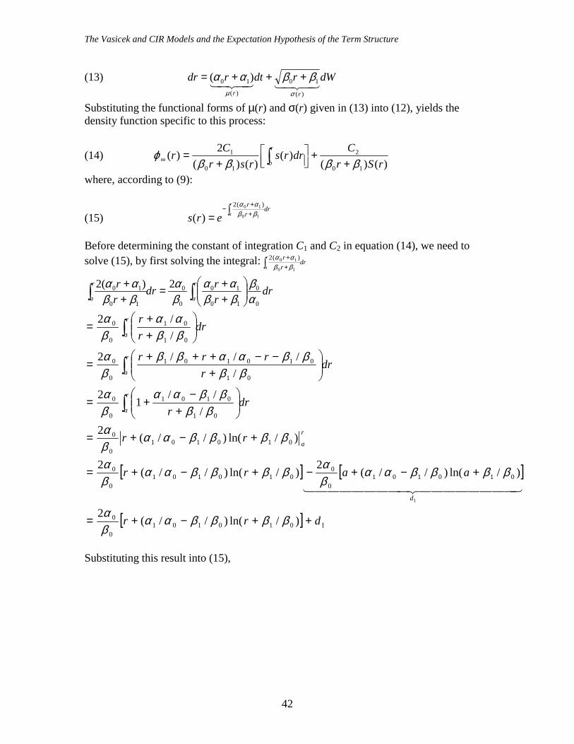
The Vasicek and CIR Models and the Expectation Hypothesis of the Term Structure
42
(13) dWrdtrdrrr4342143421)(
10
)(
10 )(σµ
ββαα +++=
Substituting the functional forms of µ(r) and σ(r) given in (13) into (12), yields the density function specific to this process:
(14) )()(
)()()(
2)(
10
2
10
1
rSrCdrrs
rsrCr
r
b ββββϕ
++
+= ∫∞
where, according to (9):
(15) dr
rrr
aers ∫= +
+−
10
10 )(2
)( ββαα
Before determining the constant of integration C1 and C2 in equation (14), we need to solve (15), by first solving the integral: dr
rrr
a∫ ++
10
10 )(2ββαα
drrrdr
rr r
a
r
a0
0
10
10
0
0
10
10 2)(2αβ
ββαα
βα
ββαα
∫∫
++=
++
[ ] [ ]
[ ] 10101010
0
0101010
0010101
0
0
0101010
0
01
0101
0
0
01
010101
0
0
01
01
0
0
)/ln()//(2
)/ln()//(2
)/ln()//(2
)/ln()//(2
///
12
////2
//2
1
drr
aarr
rr
drr
drr
rrr
drrr
d
r
a
r
a
r
a
r
a
++−+=
+−+−+−+=
+−+=
+
−+=
+
−−+++=
++
=
∫
∫
∫
ββββααβα
ββββααβαββββαα
βα
ββββααβα
ββββαα
βα
ββββααββ
βα
ββαα
βα
44444444 344444444 21
Substituting this result into (15),

The Vasicek and CIR Models and the Expectation Hypothesis of the Term Structure
43
[ ]
{
−
−−
−+−−−
−+−−−
−+−+−
+=
=
=
=
0
1
0
1
0
0
0
0
1
1010101
0
0
0
0
10101010
0
0
0
10101010
0
2
0
12
1
)/ln()//(22
)/ln()//(22
)/ln()//(2
)(
ββ
αα
βα
βα
ββββααβα
βα
ββββααβα
βα
ββββααβα
ββreD
ee
e
ers
r
D
drr
drr
drr
Equation (15) is thus transformed into
(16) 0
1
0
11)(
BrB reDrs
−
+=
ββ
where:
020
01 f
βα−=B
( )20
10
0
1
0
1
0
1
0
00
220
2β
βαβα
ββ
αα
βα
−=
−= fB
[ ])/ln()//(2
1
0101010
0
1ββββαα
βα
+−+− ==
aad eeD
Using (16), and the fact that:
+
+=
+
+=
+
−−+−
0
10
0
1
0
1
0
1
1
0
1000
βββ
ββ
ββ
ββ
ββ r
rrrrBBB
the density function (14) can be successively rewritten as:
0
1
0
1
0
1
0
1110
2
0
11
0
1110
1
)()(
2)( BrB
r
b
BrB
BrB reDr
CdrreD
reDr
Cr −
−
−∞
++
+
+
++
= ∫ββββ
ββ
ββββ
ϕ
1
0
110
2
0
111
0
110
10
1
0
1
0
1
2)( +−
−
+−∞
+
+
+
+
= ∫ BrB
r
b
BrB
BrB reD
CdrreD
reD
Cr
βββ
ββ
βββ
ϕ

The Vasicek and CIR Models and the Expectation Hypothesis of the Term Structure
44
(18) 1
0
110
2
0
11
0
10
10
1
0
1
0
1
2)( +−
−
+−∞
+
+
+
+
= ∫ BrB
r
b
BrB
BrB reD
Cdrre
re
Cr
βββ
ββ
βββ
ϕ
We finally are in position to evaluate the constant of integration in (18). First, observe that:
+∫
−
brbr
drrer
b
BrB
pp
ff
for 0for 00
1
0
1
ββ
Ensuring 0)( ≥∞ rϕ for all possible r therefore requires setting C1=0, such that the density function becomes:
1
0
1
10
21
0
110
20
1
0
1
)(−
−+−∞
+=
+
=B
rBB
rB
reD
C
reD
Crββ
β
βββ
ϕ
which, using that 0
11
0
1111 β
βββ BBrBrB +−−=− , implies:
(19) 1
0
1
2
1
0
1
1
10
2
0
0
11
0
0
11
2
10
1
1)(
)(
−
+−
∞
−
+−
∞
+=
+=
BrB
BrB
D
reD
r
reeD
Cr
ββϕ
ββ
βϕ
ββ
βββ
ββ
43421
Second, recalling that: 1)( =∫+∞
∞− ∞ drrϕ , successively yields, by integrating (19):
drreD
drreD
drr
BrB
BrB
∫
∫∫
∞
∞−
−
+−
∞
∞−
−
+−∞
∞− ∞
+=
⇒
=
+=
1
0
12
1
0
1
2
0
0
11
0
0
11
11)(
ββ
ββϕ
ββ
ββ
As shown above, for a solution in R, the affine model imposes that 0
1
ββ
−≥r .
Consequently, changing the lower limit of integration:
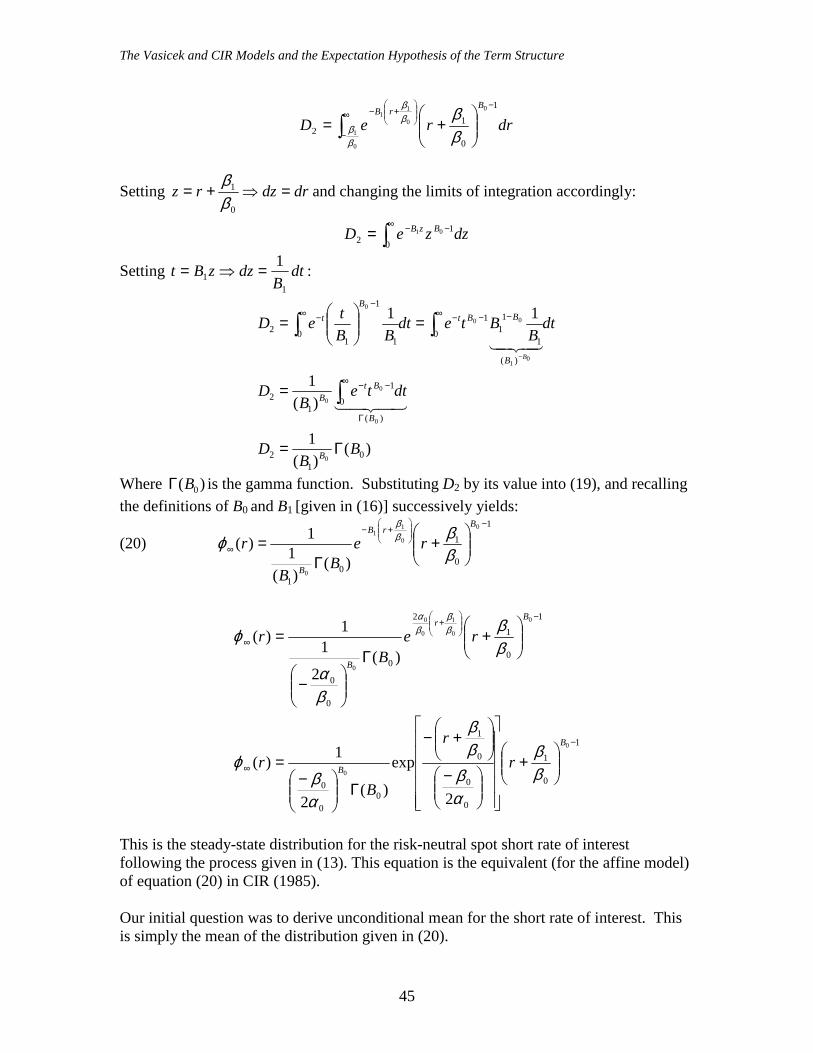
The Vasicek and CIR Models and the Expectation Hypothesis of the Term Structure
45
drreDB
rB
∫∞
−
−
+−
+=
0
1
0
0
11
1
0
12
ββ
ββ
ββ
Setting drdzrz =⇒+=0
1
ββ
and changing the limits of integration accordingly:
dzzeD BzB∫∞ −−=0
12
01
Setting dtB
dzzBt1
11=⇒= :
)()(
1
)(1
11
01
2
)(
0
1
12
0
)(
1
11
1
01
1
12
0
0
0
0
01
00
0
BB
D
dtteB
D
dtB
BtedtBB
teD
B
B
BtB
B
BBtB
t
B
Γ=
=
=
=
Γ
∞ −−
∞ −−−∞−
−
∫
∫∫−
43421
43421
Where )( 0BΓ is the gamma function. Substituting D2 by its value into (19), and recalling the definitions of B0 and B1 [given in (16)] successively yields:
(20) 1
0
1
01
0
0
11
0)(
)(1
1)(−
+−
∞
+
Γ=
BrB
B
reB
B
rββϕ β
β
1
0
1
0
0
0
1
00
0
1
0
1
2
0
0
0
0
0
0
0
1
0
0
0
2
exp
)(2
1)(
)(2
11)(
−
∞
−
+
∞
+
−
+−
Γ
−=
+
Γ
−
=
B
B
Br
B
rr
B
r
reB
r
ββ
αβ
ββ
αβ
ϕ
ββ
βα
ϕ ββ
βα
This is the steady-state distribution for the risk-neutral spot short rate of interest following the process given in (13). This equation is the equivalent (for the affine model) of equation (20) in CIR (1985). Our initial question was to derive unconditional mean for the short rate of interest. This is simply the mean of the distribution given in (20).

The Vasicek and CIR Models and the Expectation Hypothesis of the Term Structure
46
Observe that if a variable 0
1
ββ
+= rz follows a Gamma distribution given by:
(21) ( ) ( ) 1
0
00
0
0
0
0
2
exp
)(2
1)( −∞
−−
Γ
−= B
B zz
B
z
αβ
αβ
ϕ
its mean (first moment) would be given by [see Ramanathan (1993)]:
( )
−
−=
− 2
0
10
0
1
0
00
0
0 2222 β
βαβα
αβ
αβ
B
Although the r.h.s. term in (21) is equal to the r.h.s. term in (20), what we want to obtain is the mean of r, not the mean of z. But this is easily obtain because
0
1
0
1 )()(ββ
ββ
−=⇒+= zErErz
The short rate r thus has an unconditional mean given by:
( ) 0
12
0
10
0
1
0
0 222 β
ββ
βαβα
αβ −
−− .
This can finally be simplified as 0
1
αα
− , which is the result stated initially in equation (6)
above.

The Vasicek and CIR Models and the Expectation Hypothesis of the Term Structure
47
A4. The Affine model (with Yanjun Liu)
The affine model (Duffie and Kan 1996) is described as follows in appendix A3:
rBAetrP )()())(,( τττ −=
(1) γαγ
τ γτ
γτ
2)1)(()1(2)(
0 +−−−=
eeB
(2)
−
++
−+
−+
−=
−= ∫
γτβγαγβ
γτ
βα
βαβτ
βαγα
βαγβ
ττατβττ
21
)(1)(2
2)(ln22
21
)()(21)(
20
01
0
120
01
0
01
2
0
01
0 12
1
g
g
dBBA
where: 02
0 2βαγ +=
and: γαγτ γτ 2)1)(()( 0 +−−= eg The boundary conditions are given by the fact that a bond has a terminal value (when τ=0) of P(T,T)=P(0) =1, such that, given (6) in Appendix A1:
0)0()0(1)0( )0()0(
==⇒== −
BAeP rBA
In this appendix, we show how to derive equations (1) and (2) above. We saw in Appendix A1 that in the Vasicek model we had to integrate two ordinary differential equations given by equations (8) and (9) of that appendix: 1)()(' =+ ττ kBB and:
( ) 0)(2
)()(' 22
=+−−− τστσλϑτ BBkA
Similarly, the more general affine model requires integrating two differential equations given by:
(3) 12
)()()('
20
0 −=−+−τβτατ BBB
and:

The Vasicek and CIR Models and the Expectation Hypothesis of the Term Structure
48
(4) 0)(21)()(' 2
11 =+−− τβτατ BBA
Box 2 shows how to obtain equations (3) and (4). The procedure is similar to the one used in Appendix 1 and thus requires little explanation. These two differential equations (3) and (4) are labeled equation (21) in Bolder (2001) and can also be found, for example, in Wilmott (1998) (equations 33.12 and 33.13). However, none of these authors provide any details on finding a solution to these two ordinary differential equations. Wilmott simply gives the solution in the form of equation (1) and (2) above. Bolder integrates special cases of (3) and (4). For the Vasicek model, he postulates that: 2
1010 ;0 ; ; σββσλϑαα ==−=−= kk , while for the CIR model, he postulates that: 0 ; ; );( 1
2010 ===+−= βσβϑαλα kk . Bolder substitutes these
parameters into (3) and (4) and integrates these specific and much easier ordinary differential equations to obtain the Vasicek and CIR versions of the affine model. (Note for example that by substituting 2
1010 ;0 ; ; σββσλϑαα ==−=−= kk into (3) and (4), we re-obtain the differential equations (8) and (9) of Appendix A1.) In this appendix we show how to integrate (3) and (4) instead of integrating specific cases as done in Bolder (2001). We are not aware of any other source which presents these derivations in any detail. Rewriting (3) as:
(5)
τβ
βτ
βατ
τβ
τβατβ
ττ
τβτατ
dBB
dB
BBd
dB
BBB
0
00
02
00
020
200
21
2)(2
)(
)(
2)(2
)(21)(
)(21)(1)('
−=−−
⇒
−−−=⇒
−+=
Let us define:
(6)
0
0200
2
0
0200
1
2
2
ββαα
ββαα
+−≡
++≡
X
X
Using (6), observe that:

The Vasicek and CIR Models and the Expectation Hypothesis of the Term Structure
49
Box 2. Deriving the differential equations (3) and (4) Following the equations of Appendix A1 (and re-labelling them with an added prime), we can establish that if the short-rate follows the process: (1’) dWfdttdr ρ+=)( we obtain, using Itôs lemma that:
(2’) dWPdtfPPPtrTtdP rrrrt ρρ +
++= 2
21))(,,(
and so:
(3’) {
dWPPdt
P
fPPP
trTtPtrTtdP
PdPPdP
rrrrt
//
2
21
))(,,())(,,(
σµ
ρρ
+
++
=444 3444 21
Substituting (3’) into equation (B4) of Box 1, Appendix 1, yields:
(B5’) ( ) 0)(2
)(2
=−+−+ PtrPPtfP rrrtρρλ .
Substituting equation (7), Appendix 1 into (B5’), yields:
( ) ( ) 0)('1)(2
)()(' 22
=−−+−−− ττρτρλτ BrBBfA
To solve this partial differential equation, we should note that until now, the process in (1’) was written without specifying the drift f or the volatility ρ. The affine model specifies the drift and the volatility such that we can actually solve this partial differential equation explicitly. The affine model assumes that:
10
10
ββρ
ααρλ
+=
+=−
r
rf
such that the partial differential equation becomes:
02
)()()('1()(
21)()('
20
02
11 =
−+−−+−− r
BBBBBA
τβταττβτατ ,
which implies that equations (3) and (4) of this appendix must hold.

The Vasicek and CIR Models and the Expectation Hypothesis of the Term Structure
50
( )( )
00
02
20
020
2
0
0
0
02
0
020
0
0
0
020
0
0
0
02
210
020
0
0
0
020
0
02
21122
21
2)(2
)(
2)(2)(
22)(2)(
2)()(2)()()(
)()()()()(
βτ
βατ
ββα
βα
βτατ
ββα
βα
ββα
βα
βτατ
ββατ
βατ
ββατ
βαττ
τττττ
−−=
+−
+−=
+−
+++−=
++
−−+
+−=
+−−=−−
BB
BB
BB
XXBBBB
B
XXXBXBBXBXB
We can thus rewrite (5) as:
( )( ) τβττ
τ dXBXB
dB0
21 21
)()()( −=
−−
Using the fact that:
( )( )
−
−−−
=−− 121221 )(
1)(11
)()(1
XBXBXXXBXB ττττ
we can rewrite the differential equation as:
τβτττ
ddBXBXBXX 0
1212 21)(
)(1
)(11 −=
−
−−−
Recalling the derivative rules:
( ) ( )1
1
2
2
)(1)(ln
;)(1)(ln
XBdBBXd
XBdBXBd
−=
−−
=−
ττ
ττ
this implies:
( ) ( )( )
τβτ
τ
τβττ
dXXBX
XBd
dBXdXBdXX
021
1
2
01212
2)()(ln
21)(ln)(ln1
−=
−
−⇒
−=−−−−
Integrating the above expression:

The Vasicek and CIR Models and the Expectation Hypothesis of the Term Structure
51
)0(2)0(
)0(ln
)()(
ln
2)()(ln
2)()(
ln
021
1
2
1
2
0021
01
2
0021
01
2
−−
=
−
−−
−
−⇒
−=
−
−⇒
−=
−
−∫∫
τβτ
τ
τβτ
τ
τβτ
τ
ττ
ττ
XXBX
XBBX
XB
XXBX
XB
dXXBX
XBd
Recalling the boundary conditions that B(0) =0:
τβττ
τβτ
τ
021
2
1
1
2
021
1
2
1
2
2)()(
ln
2ln
)()(ln
XXXX
XBXB
XXXX
BXXB
−=
−−
⇒
−=
−−
−
−
Recalling the definitions of X1 and X2 given in (6), yields:
(7)
( )
2
2
1
2
2
212
211
020
2
1
1
2
111)(
)()(
2)()(ln
020
020
020
Xe
X
eB
eXXXBXXXB
XX
XBXB
−
−=⇒
=−−
⇒
+=
−−
+
+
+
τβα
τβα
τβα
τ
ττ
τβαττ
We defined in (2) that γβα =+ 020 2 . Thus, using (6):
(8a) ( )( )
200
0αγαγβ +−
=
(8b) 2
1 0
0
0
1
αγγα
β −=
+=
X
(8c) 2
1 0
0
0
2
αγγα
β +−=
−=
X
Substituting (8) into B(τ) given in (7) yields:

The Vasicek and CIR Models and the Expectation Hypothesis of the Term Structure
52
(9)
γαγαγ
αγαγ
αγαγτ
γτ
γτ
γτ
γτ
γτ
γτ
τβα
τβα
2)()()1(2
)()1(2
22
111
1)(
00
00
00
2
2
1
2
020
020
+−−−−=
++−−=
++
−−=
−
−=
+
+
ee
ee
e
e
Xe
X
eB
And hence, we obtain our solution for B(τ) given in (1) and rewritten here as:
(10) γαγ
τ γτ
γτ
2)1)(()1(2)(
0 +−−−=
eeB
Now it remains to obtain A(τ) by solving equation (4):
(11)
∫∫
−==⇒
−=⇒
=+−−
ττττατβτ
τττ
τατβττ
τβτατ
0 12
10
12
1
211
)()(21)()(
)()(21)(
0)(21)()('
dBBdd
dAA
BBd
dA
BBA
To solve this integral, we thus have to use the solution derived above for B(τ). It is easier to transform B(τ) as follows:
(12) )(
)1(22)1)((
)1(2)(0 τγαγ
τγτ
γτ
γτ
ge
eeB −=
+−−−=
such that:
(13) γτ
γτ
γαγτγγαγτ
eggeg
)()('
2)0(2)1)(()(
0
0
−=
=⇒+−−=
and so:
(14) ( ) )()()()()('
)()(')()()(
00
000
γαγτγγατγτ
γαγτγααγτ γτ
+−=+−=⇒
++=++−=
ggg
geg
Now recall that we obtained above under (8a) that:
The Vasicek and CIR Models and the Expectation Hypothesis of the Term Structure
53
( )( ) ( )( )0
00000 2
2 βαγαγαγαγβ +−
=⇒+−
=
This permits us to rewrite B(τ) in (12) as:
(15)
( )( )
( ) ( ))(
)1(
)()1(
)()1(2
2)1)(()1(2)(
0
0
0
0
00
0
ταγ
βαγ
τβαγαγ
τγαγτ
γτ
γτγτ
γτ
γτ
ge
ge
ge
eeB
−+−=
−+−=−=
+−−−=
Observe also that:
44 344 2144 344 21
(13) using
0(13) using
00)('2)(2)()1(2)1)(()1)((
αγττγτγαγαγ γτγτγτγτ
−+−=+−=−+−+−=−+ ggegeee
so that:
(16)
+
−−=
⇒
−
+−−
=−
+−−
=
)()('2)(
)()('21
)(
)('2)(
)(
00
0
00
00
0
0
ττ
ββαγ
τ
ττ
αγβαγ
ταγττ
βαγ
τ
ggB
gg
g
ggB
Recall that our objective is to solve equation (11) above. We thus want to substitute B(τ) and B2(τ) in that equation. Therefore:
(17) ( )0
0
02
2
20
2
0
02 )()()('4
)()('4)(
βαγ
ττ
βττ
ββαγτ −
−+
−=
gg
ggB
Now, we also know that:
( ) ( ))(
)(')()()('
)()()()('
)()(')('
)()('
20
(14) using
20
22
2
ττγαγ
ττγ
τγαγτγτ
τττ
ττ
gg
gg
ggg
ggg
gg +
−=+−
==4444 34444 21
so that equation (17) can now be rewritten as:

The Vasicek and CIR Models and the Expectation Hypothesis of the Term Structure
54
(18)
)()('4
)()(')(4
)(
)()()('4
)()(')(
)()('4)(
20
022
0
0
2
0
02
0
0
02
020
2
0
02
ττ
βα
ττ
βγαγ
βαγτ
βαγ
ττ
βττγαγ
ττγ
ββαγτ
gg
ggB
gg
gg
ggB
++
−
−=
−−
+−+
−=
We can now substitute B(τ) given in (16) and B2(τ) given in (18) into (11):
∫
−=
τττατβτ
0 12
1 )()(21)( dBBA
Note that the expression in brackets can be expressed as:
)()(')(2
)()('22
21
)()('2
)()('2
)()(')(2
21
)()(21
220
01
0
120
01
0
01
2
0
01
01
0
012
0
0122
0
01
2
0
01
12
1
ττ
βγαγβ
ττ
βα
βαβ
βαγα
βαγβ
ττ
βα
βαγα
ττ
βαβ
ττ
βγαγβ
βαγβ
τατβ
gg
gg
gg
gg
gg
BB
+−
−+
−+
−=
−
−++
+−
−=
−
and thus:
(19)
∫
∫∫
∫
+−
−+
−+
−=
−=
τ
ττ
τ
τττ
βγαγβ
τττ
βα
βαβτ
βαγα
βαγβ
ττατβτ
0 220
01
00
120
01
00
01
2
0
01
0 12
1
)()(')(2
)()('22
21
)()(21)(
dgg
dggd
dBBA
Now observe that:
=−=== ∫∫ γ
τττττττ τ ττ
2)(ln)0(ln)(ln)(ln)(ln
)()('
0 00
gggggddgg
if we recall that g(0)=2γ [see equation (13)]. As well, setting a change of variable:

The Vasicek and CIR Models and the Expectation Hypothesis of the Term Structure
55
1)()()( ==⇒=⇒=ττ
ττττττ
dd
ddgdgdg
yields:
−−=+−=−=−−== ∫ ∫∫ γττττ
τττ
ττ ττ
21
)(1
)0(1
)(11
)(1
)(1
)()('
)(
)0(2
)(
)0(
)(
)0(20 2 ggggdg
gdg
gd
gg
g
g
g
g
g
g
and thus, substituting the results above into (19):
(20)
−
++
−+
−+
−=
−= ∫
γτβγαγβ
γτ
βα
βαβτ
βαγα
βαγβ
ττατβττ
21
)(1)(2
2)(ln22
21
)()(21)(
20
01
0
120
01
0
01
2
0
01
0 12
1
g
g
dBBA
which is equation (2) above.
In the last step, we show that the affine model is a general case of the CIR model. To see this, simply define that:
(21)
==
=+−=
0 ;
; );(
1
20
1
0
βσβϑα
λαk
k
Substituting these parameter values into (1), yields:
(22) γλγγαγ
τ γτ
γτ
γτ
γτ
2)1)(()1(2
2)1)(()1(2)(
0 +−++−=
+−−−=
eke
eeB
where 220
20 2)(2 σλβαγ ++=+= k
This corresponds to the first part of equation (29) in Bolder (2001). The second part can be recovered as follows by substituting again the parameter values defined in (21) into equation (2):
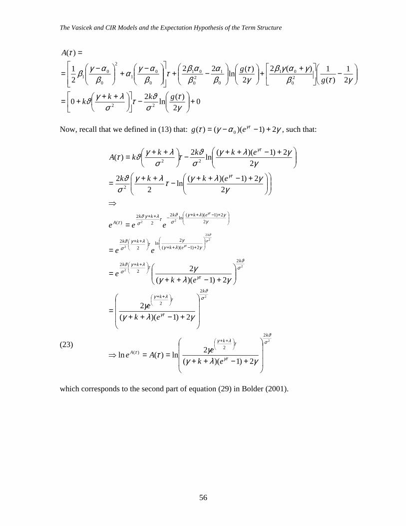
The Vasicek and CIR Models and the Expectation Hypothesis of the Term Structure
56
02
)(ln20
21
)(1)(2
2)(ln22
21
)(
22
20
01
0
120
01
0
01
2
0
01
+
−
+++=
−
++
−+
−+
−=
=
γτ
σϑτ
σλγϑ
γτβγαγβ
γτ
βα
βαβτ
βαγα
βαγβ
τ
gkkk
gg
A
Now, recall that we defined in (13) that: γαγτ γτ 2)1)(()( 0 +−−= eg , such that:
(23) 2
2
22
22
2
22
2
2)(
2
2
2
22
2)1)((2ln
22
22)1)((ln2
22
)(
2
22
2)1)((2ln)(ln
2)1)((2
2)1)((2
22)1)((ln
22
22)1)((ln2)(
σϑ
γτ
τλγ
τ
σϑ
γτ
τλγ
σϑ
γτ
τλγσ
ϑ
γλγγ
τλγσ
ϑ
γγλγ
σϑ
τλγσ
ϑτ
γτ
γτ
γλγγτ
γλγγ
γλγγ
γγλγτλγ
σϑ
γγλγ
σϑτ
σλγϑτ
σ
ϑ
γτ
γτ
kk
A
kk
kkk
ekkk
ekkkkA
ekeAe
eke
eke
ee
eee
ekkk
ekkkkA
k
+−++==⇒
+−++=
+−++
=
=
=
⇒
+−++−++=
+−++−
++=
++
++
++
+−++
++
+−++−++
which corresponds to the second part of equation (29) in Bolder (2001).

The Vasicek and CIR Models and the Expectation Hypothesis of the Term Structure
57
A5. Coding the Vasicek model This appendix provides the code for three files that can be used in Portable Troll to simulate the Vasicek model. The first two files are input files and the third is a macro. The first input file describes the parameters of the model presented in Table 1 of the paper. The second input file describes the Vasicek model as explained in Appendix A1. Finally, the macro is used to simulate the Vasicek model over a 10-year horizon and for a large number of times or runs (RNS=500). The reader can simply copy and save these files as, respectively, Param.inp, Vasicek.inp. and Simulate.src. Then, in the Troll input window, simply type: Input Param; Input Vasicek; Compile Simulate; &Simulate This should launch the simulation. Once the simulation is done, (which takes about 5 seconds for one single run), the reader may want to plot some results into the Troll environment, by typing into the input window, say: &plot variable out_dat_I_1 out_dat_I_4 out_dat_I_8 out_dat_I_20 out_dat_I_80, range 2001q1 to 2011q4; This should give a plot for I_1, …, I_80, the one-quarter …, 80-quarter interest rates, over a 10-year horizon for the particular “run” chosen. From this, we can observe (vertically) a yield curve for each quarter of the 10-year horizon and observe how the shape of the yield curve evolves over the ten-year horizon. //Param.inp //Benchmark parameter value for the Vasicek model: Table 1, in this paper access benchmark type trolldb id "param.trd" mode c; search benchmark w; dofile k = 0.147; //k = mean reverting speed dofile theta = 0.074; //theta = mean reverting level of the short rate dofile sigma = 0.029; //sigma = volatility dofile lambda = -0.154; //market price of risk dofile thetabar = theta - sigma*lambda/k; // (=0.10438) upper bound in Vasicek dofile gamma = ((k**2)*thetabar)-(sigma**2)/2; dofile tau = 0.25; //tau = time to maturity = T-t dofile dt = 1/4; //Continuous-time process approximated to quarterly time interval delsearch all; delaccess all; //Vasicek.inp // The Vasicek model as described in Appendix 1 usemod; addsym

The Vasicek and CIR Models and the Expectation Hypothesis of the Term Structure
58
endogenous Rinst B_800 B_80 B_40 B_20 B_12 B_8 B_4 B_2 B_1 A_800 A_80 A_40 A_20 A_12 A_8 A_4 A_2 A_1 P_800 P_80 P_40 P_20 P_12 P_8 P_4 P_2 P_1 I_800 I_80 I_40 I_20 I_12 I_8 I_4 I_2 I_1 , parameter k theta sigma lambda thetabar gamma tau dt; addeq bottom //process for "instantaneous" very short rate, rinst (noted r in this paper) //See Footnote 2 in this paper rinst = theta + (rinst(-1)-theta)*exp(-k*dt) + sqrt(((sigma**2)/2*k)*(1-exp(-2*k*dt)))*e1, // for one-quarter maturity instrument B_1 = (1 - Exp(-k*tau)) / k, //See Equation (10) Appendix 1 A_1 = (Gamma*(B_1-tau)/k**2)-((sigma**2)*(B_1**2))/(4*k), //See Equation (11) Appendix 1 P_1 = Exp(A_1-B_1*rinst), //See Equation (6) in Appendix 1 I_1 = (-(Log(P_1) / Log(2.718282)) / (tau))*100, //See Equation (12) in Appendix 1. //note: change of notation: I in code = z in paper. //example: I_1 = z(1/4), i.e., the interest rate on a one-quarter maturity instrument //note: natural log in paper are transformed into basis 10 log in code. See Chiang (1984), p 291. //for 2-quarters maturity instrument B_2 = (1 - Exp(-k*tau*2)) / k, A_2 = (Gamma*(B_2-tau*2)/k**2)-((sigma**2)*(B_2**2))/(4*k), P_2 = Exp(A_2-B_2*rinst), I_2 = (-(Log(P_2) / Log(2.718282)) / (tau*2))*100, // for 1-year maturity instrument B_4 = (1 - Exp(-k*tau*4)) / k, A_4 = (Gamma*(B_4-tau*4)/k**2)-((sigma**2)*(B_4**2))/(4*k), P_4 = Exp(A_4-B_4*rinst), I_4 = (-(Log(P_4) / Log(2.718282)) / (tau*4))*100, B_8 = (1 - Exp(-k*tau*8)) / k, A_8 = (Gamma*(B_8-tau*8)/k**2)-((sigma**2)*(B_8**2))/(4*k), P_8 = Exp(A_8-B_8*rinst), I_8 = (-(Log(P_8) / Log(2.718282)) / (tau*8))*100, B_12 = (1 - Exp(-k*tau*12)) / k, A_12 = (Gamma*(B_12-tau*12)/k**2)-((sigma**2)*(B_12**2))/(4*k), P_12 = Exp(A_12-B_12*rinst), I_12 = (-(Log(P_12) / Log(2.718282)) / (tau*12))*100, B_20 = (1 - Exp(-k*tau*20)) / k, A_20 = (Gamma*(B_20-tau*20)/k**2)-((sigma**2)*(B_20**2))/(4*k), P_20 = Exp(A_20-B_20*rinst), I_20 = (-(Log(P_20) / Log(2.718282)) / (tau*20))*100, B_40 = (1 - Exp(-k*tau*40)) / k, A_40 = (Gamma*(B_40-tau*40)/k**2)-((sigma**2)*(B_40**2))/(4*k), P_40 = Exp(A_40-B_40*rinst), I_40 = (-(Log(P_40) / Log(2.718282)) / (tau*40))*100, B_80 = (1 - Exp(-k*tau*80)) / k, A_80 = (Gamma*(B_80-tau*80)/k**2)-((sigma**2)*(B_80**2))/(4*k), P_80 = Exp(A_80-B_80*rinst), I_80 = (-(Log(P_80) / Log(2.718282)) / (tau*80))*100, //The following is for a 200-year maturity instrument: //This is supposed to illustrate the long-term properties of the model that //the zero-coupon rate on a very long-term rate is deterministic and tends to gamma/(k**2) B_800 = (1 - Exp(-k*tau*800)) / k, A_800 = (Gamma*(B_800-tau*800)/k**2)-((sigma**2)*(B_800**2))/(4*k), P_800 = Exp(A_800-B_800*rinst), I_800 = (-(Log(P_800) / Log(2.718282)) / (tau*800))*100,

The Vasicek and CIR Models and the Expectation Hypothesis of the Term Structure
59
; filemod vasicek; //Simulate.src //Macro to simulate the vasicek model Addfun Main; Procedure Main () Begin; ×ecs ; >> on >>Delsearch all; >>Delaccess all; >>sysopt log off; >>ACCESS BASE TYPE TROLLDB ID "MAIN.TRD" MODE c; //The shape of the yield curve depends on the value of the short rate (rinst) relative to some bounds //The following 4 lines give four different starting point for rinst and thus four different intial shapes for yield curves. //Use only one of the four lines below, comment out the 3 others using double bars // and experiment!!! >>dofile base_rinst = RESHAPE(CRMAT(400, 1, 0.12), 1961Q1); // This should provide an initially inverted yield curve with //existing parameter set //>>dofile base_rinst = RESHAPE(CRMAT(400, 1, 0.095), 1961Q1); // Humped-shaped //>>dofile base_rinst = RESHAPE(CRMAT(400, 1, 0.084921), 1961Q1); //Humped-shaped //>>dofile base_rinst = RESHAPE(CRMAT(400, 1, 0.074), 1961Q1); // This should initially yield an upward sloping yield curve >>DOFILE BASE_B_800 = RESHAPE(CRMAT(400, 1, 0), 1961Q1); >>DOFILE BASE_A_800 = RESHAPE(CRMAT(400, 1, 0), 1961Q1); >>DOFILE BASE_P_800 = RESHAPE(CRMAT(400, 1, 0), 1961Q1); >>dofile base_I_800 = reshape(crmat(400, 1, 0), 1961q1); >>DOFILE BASE_B_80 = RESHAPE(CRMAT(400, 1, 0), 1961Q1); >>DOFILE BASE_A_80 = RESHAPE(CRMAT(400, 1, 0), 1961Q1); >>DOFILE BASE_P_80 = RESHAPE(CRMAT(400, 1, 0), 1961Q1); >>dofile base_I_80 = reshape(crmat(400, 1, 0), 1961q1); >>DOFILE BASE_B_40 = RESHAPE(CRMAT(400, 1, 0), 1961Q1); >>DOFILE BASE_A_40 = RESHAPE(CRMAT(400, 1, 0), 1961Q1); >>DOFILE BASE_P_40 = RESHAPE(CRMAT(400, 1, 0), 1961Q1); >>dofile base_I_40 = reshape(crmat(400, 1, 0), 1961q1); >>DOFILE BASE_B_20 = RESHAPE(CRMAT(400, 1, 0), 1961Q1); >>DOFILE BASE_A_20 = RESHAPE(CRMAT(400, 1, 0), 1961Q1); >>DOFILE BASE_P_20 = RESHAPE(CRMAT(400, 1, 0), 1961Q1); >>dofile base_I_20 = reshape(crmat(400, 1, 0), 1961q1); >>DOFILE BASE_B_12 = RESHAPE(CRMAT(400, 1, 0), 1961Q1); >>DOFILE BASE_A_12 = RESHAPE(CRMAT(400, 1, 0), 1961Q1); >>DOFILE BASE_P_12 = RESHAPE(CRMAT(400, 1, 0), 1961Q1); >>dofile base_I_12 = reshape(crmat(400, 1, 0), 1961q1); >>DOFILE BASE_B_8 = RESHAPE(CRMAT(400, 1, 0), 1961Q1); >>DOFILE BASE_A_8 = RESHAPE(CRMAT(400, 1, 0), 1961Q1); >>DOFILE BASE_P_8 = RESHAPE(CRMAT(400, 1, 0), 1961Q1); >>dofile base_I_8 = reshape(crmat(400, 1, 0), 1961q1); >>DOFILE BASE_B_4 = RESHAPE(CRMAT(400, 1, 0), 1961Q1); >>DOFILE BASE_A_4 = RESHAPE(CRMAT(400, 1, 0), 1961Q1); >>DOFILE BASE_P_4 = RESHAPE(CRMAT(400, 1, 0), 1961Q1); >>dofile base_I_4 = reshape(crmat(400, 1, 0), 1961q1); >>DOFILE BASE_B_2 = RESHAPE(CRMAT(400, 1, 0), 1961Q1); >>DOFILE BASE_A_2 = RESHAPE(CRMAT(400, 1, 0), 1961Q1); >>DOFILE BASE_P_2 = RESHAPE(CRMAT(400, 1, 0), 1961Q1); >>dofile base_I_2 = reshape(crmat(400, 1, 0), 1961q1);

The Vasicek and CIR Models and the Expectation Hypothesis of the Term Structure
60
>>DOFILE BASE_B_1 = RESHAPE(CRMAT(400, 1, 0), 1961Q1); >>DOFILE BASE_A_1 = RESHAPE(CRMAT(400, 1, 0), 1961Q1); >>DOFILE BASE_P_1 = RESHAPE(CRMAT(400, 1, 0), 1961Q1); >>dofile base_I_1 = reshape(crmat(400, 1, 0), 1961q1); >>DELACCESS ALL; >>DELSEARCH ALL; SDATE = 2001Q1; QRT = 44; cqrt = 152; //RNS below implies that there will be 500 simulations of a 44 quarters time horizon RNS = 500; NAMES=COMBINE("B_800","B_80","B_40","B_20","B_12","B_8","B_4","B_2","B_1", "A_800","A_80","A_40","A_20","A_12","A_8","A_4","A_2","A_1", "P_800","P_80","P_40","P_20","P_12","P_8","P_4","P_2","P_1", "I_800","I_80","I_40","I_20","I_12","I_8","I_4","I_2","I_1", "rinst"); NUM=NVALS(NAMES); nshks=combine("e1"); nums=nvals(nshks); >>access par type trolldb id "param.trd"; >>access base type trolldb id "Main.trd" mode o; >>access vas type trolldb id "vasicek.trd" mode c; >>access out type trolldb id "outdata.trd" mode c; >>access shk type trolldb id "shocks.trd" mode c; >>access mat type trolldb id "gm.trd" mode c; for (K=1; K<=num; k=k+1) { name=names[K]; >>do mat_&(name)=crmat(&qrt,0); } //introduction of shocks //To generate 500 simulations of the same 44 quarters horizon write instead // For (X=1; X<=RNS; X=X+1), otherwise experiment with the following line For (X=1; X<=1; X=X+1) { >>do shk_vec_e1 = randnorm(1262+&x,9783-&X,base_rinst); FOR (K=1; K<=NUM; K=K+1) { NAME=NAMES[K]; >>DO OUT_DAT_&(NAME)=BASE_&(NAME); } FOR (qq=SDATE; qq<=SDATE+QRT-1; qq=qq+1) { FOR (S=1; S<=NUMS; S=S+1) { NSHK=NSHKS[S]; >>DO SHK_&(NSHK)=OVERLAY(SUBRANGE(SHK_vec_&(NSHK),&qq,&QQ),RESHAPE(CRMAT(&CQRT*2,1,0),&SDATE-7)); } >>DO PRINT("vas",":","QQ","RUN",":",&X); >>DELSEARCH ALL; >>SEARCH FIRST shk OUT_DAT PAR base; >>USEMOD vasicek; >>CONOPT CONCR 0.0001 STOP 100; >>SIMULATE OLDSTACK 50; >>SIMSTART &qq; >>DOSTACK 1;

The Vasicek and CIR Models and the Expectation Hypothesis of the Term Structure
61
>>FILESIM vas; FOR (K=1; K<=NUM; K=K+1) { NAME=NAMES[K]; >>DOFILE OUT_DAT_&(NAME)=OVERLAY(vas_&(NAME),OUT_DAT_&(NAME)); } } FOR (K=1; K<=NUM; K=K+1) { NAME=NAMES[K]; >>DO MAT_&(NAME)=ADDCOL(MAT_&(NAME),0,RESHAPE(SUBRANGE(OUT_DAT_&(NAME),&SDATE,&SDATE+&QRT-1),&QRT,1)); } >>delsearch all; } ×ecs ; >> off >>quit; end;

The Vasicek and CIR Models and the Expectation Hypothesis of the Term Structure
62
References Ang, A. and Piazzesi, M. (2001), “A no-arbitrage vector autoregression of term structure
dynamics with macroeconomic and latent variables”, NBER working paper 8363. Bernanke, B. and Blinder, A. (1992), “The federal funds rate, and the channels of
monetary transmission”, American Economic Review, 82, 901-921. Bolder, David (2001): “Affine Term-Structure Models: Theory and Implementation”,
Bank of Canada Working Paper 2001-15. Bolder, David (2002): “The Government of Canada’s Debt Strategy Simulation
Framework”, Discussion paper, Bank of Canada. Chiang, Alpha (1984): Fundamental Methods of Mathematical Economics, New York,
McGraw-Hill Book Company. Cox, John, Jonathan Ingersoll, and Stephen Ross (1981): “A Re-examination of
Traditional Hypotheses about the Term Structure of Interest Rates, The Journal of Finance, Vol. 36, No. 4, pp. 769-799.
Cox, John, Jonathan Ingersoll, and Stephen Ross (1985): “A Theory of the Term
Structure of Interest Rates”, Econometrica, Vol. 53, No. 2, pp. 385-407. Danish Nationalbank (2001): “Danish Government Borrowing and Debt 2001”, available
at: http://www.nationalbanken.dk/nb/nb.nsf/alldocs/Sdanish_government_debt_fulltext_2001/$File/Chap09.htm
Debt Management Strategy: 2003-2004, Department of Finance-Canada, available at
http://www.fin.gc.ca/purl/dms-e.html Dewachter, H. and Lyrio, M. (2003), “Macro factors and the term structure of interest
rates”, http://www.econ.kuleuven.ac.be/ew/academic/intecon/Dewachter/default.htm
Dixit, Avinash and Pindyck, Robert (1994): Investment under Uncertainty, Princeton,
Princeton University Press. Duffie D. and Kan R. (1996): “A yield-factor model of interest rates” Mathematical
Finance 6, 379-406. Estrella, A. and Hardouvelis, G. (1991), “ The term structure of interest rates in real and
monetary economies”, Journal of Economic Dynamics and Control, 19, 909-940.

The Vasicek and CIR Models and the Expectation Hypothesis of the Term Structure
63
Fama, E. (1986), “Term premiums and default premium in money markets”, Journal of Financial Economics, 17, 175-196.
Georges, Patrick (2003): “Borrowing Short- or Long-Term: Does the Government Really
Face a Trade-Off? – A Stochastic Framework For Public Debt Management, Department of Finance-Canada Working Paper # 2003-16.
Hull, J, and White, A. (1990): “Pricing Interest-Rate Derivative Securities”, The Review
of Financial Studies, 3, pp. 573-592. Maes, Konstantijn (2003), “Modeling the Term Structure of Interest Rates: Where do We
Stand?” Working Paper, Katholieke Universiteit Leuven. Mishkin, F (1990), “What does the term structure tell us about future inflation”, Journal
of Monetary Economics 25, 77-95. Ramanathan, Ramu (1993), Statistical Methods in Econometrics, San Diego, Academic
Press, Harcourt Brace Jovanovich. Vasicek, Oldrich (1977): “An Equilibrium Characterization of the Term Structure”,
Journal of Financial Economics 5, pp. 177-188. Wu, T. (2001), “Macro factors and the affine term structure of interest rate”, unpublished
working paper.