the vehicle-routing problem with delivery and back-haul …anily/publications/16.pdf · ·...

The Vehicle-Routing Problem with Delivery and Back-Haul Options

Shoshana Anily The Recanati Graduate School of Business Administration, Tel-Aviv University, Israel

In this article we consider a version of the vehicle-routing problem (VRP): A fleet of identical capacitated vehicles serves a system of one warehouse and N customers of two types dispersed in the plane. Customers may require deliveries from the warehouse, back hauls to the warehouse, or both. The objective is to design a set of routes of minimum total length to serve all customers, without violating the capacity restriction of the vehicles along the routes. The capacity restriction here, in contrast to the VRP without back hauls is compli- cated because amount of capacity used depends on the order the customers are visited along the routes. The problem is NP-hard. We develop a lower bound on the optimal total cost and a heuristic solution for the problem. The routes generated by the heuristic are such that the back-haul customers are served only after terminating service to the delivery customers. However, the heuristic is shown to converge to the optimal solution, under mildprobabilis- tic conditions, as fast as N-0.5. The complexity of the heuristic, as well as the computation of the lower bound, is U ( N ’ ) if all customers have unit demand size and O ( N 3 log N) otherwise, independently of the demand sizes. 0 1996 John Wiley & Sons, Inc.

1. INTRODUCTION

Improvement of a physical distribution system may have crucial consequences for a business’s performance. In certain sectors of the economy, transportation costs amount to a fifth (lumber and wood products) or even a quarter (petroleum, stone, clay, and glass products) of the average sales dollar; see [ 201. A careful design of the distribution system may thus yield significant cost savings to the company, usually by exploiting joint pro- curement possibilities to satisfy the needs of multiple locations. This potential for savings arises in particular in systems where goods are distributed through a fleet of vehicles com- bining visits to distinct locations into efficient routes.

The problem we study here deals with a single-period, single-warehouse distribution system with two sets of customers dispersed in the plane. The first set, denoted by D, consists of delivery customers that require a delivery of goods from the warehouse, whereas the second set, denoted by B , consists of back-haul customers that need to deliver goods from their location to the warehouse. It is possible for a customer to require both a delivery and a back haul. (Note that the literature distinguishes between back-haul customers and pickup customers: A pickup customer may deliver goods to any of the delivery customers and the warehouse. In this research we restrict ourselves to delivery and back-haul customers only.) In order to avoid excessive notation we will assume a single-commodity problem, and in Section 5 we explain the modifications needed for the multicommodity case. Each customer is characterized by its geographic location and its requirement size for either delivery or back haul. The company’s fleet of vehicles is used to deliver and back haul stock. All vehicles are assumed to have identical capacities. We use the Euclidean metric as the dis-

Naval Research Logistics, Vol. 43,415-434 (1996) Copyright 0 1996 by John Wiley & Sons, Inc. CCC 0894-069)3/96/0304 1 5-20

416 Naval Research Logistics, Vol. 43 ( 1996)

tance function between distinct locations. The objective is to design a set of routes of minimum total length that serves all customers, each route emanating from the warehouse, stopping at customers for delivery/back-haul purposes, and finally terminating at the warehouse without violating the vehicle’s capacity restriction along the route. References [ 51 and [ 161 present some heuristics that are shown to have bounded worst-case error ratios for the single-vehicle version of this problem, which is called the traveling-salesman problem with delivery and back haul (TSPDB ) . We call the multiple-vehicle version of the problem studied here the vehicle-routing problem with delivery and back-haul options ( VRPDB) .

The VRPDB has many real-life applications. References [ 71 and [ 91 describe some a p plications and review some solution techniques. The problem is faced, for example, by parcel services such as UPS: trucks load parcels at the warehouse and on their way they unload parcels at addressees and collect others from senders. All parcels collected must go through the warehouse before being delivered to the addressees. Another application, described in [ 91, deals with the grocery industry in the US: This industry has recognized the cost-cutting potential of servicing back-haul points on predominantly delivery routes. As the authors report, the industry has saved upwards of $160 million a year since 1982 on its distribution costs by allowing vehicles to collect large volumes of inbound material on their delivery routes. The motivation to study the problem in [ 161 comes from a project that provides summer vacations of two weeks for inner-city underprivileged children at volunteer families living out of town. The transportation service is made by buses and is confined to a limited number of days when some children start their vacation and others end theirs.

There is a vast literature on the vehicle-routing problem (VRP) with or without additional constraints. It is easy to see that if D = 4 or B = 4 then the VRPDB reduces to the VRP, proving that the problem is NP-hard (see [ 131). As such, exact solution methods become impractical when the problem size increases, leading to the need for heuristic solution methods whose running time is polynomial in the problem size. In recent years, much interest has arisen in heuristics whose effectiveness can be analyzed analytically. Several criteria have been adopted to gauge the effectiveness or accuracy of a heuristic method. The types of analyses that we will be using in this study include (a) worst-case performance analysis, which examines the maximum possible deviation from optimality of a given heuristic; (b) probabilistic analysis, which examines the average performance of a given heuristic under certain assumptions on the probability distribution of the data set; and (c) asymptotic analysis, which is closely related to probabilistic analysis, and establishes either the worst-case or the average performance of a given heuristic when the number of elements in the data set is sufficiently large. When the data set is random we say that heuristic H is asymptotic optimal if under certain probability distribution conditions on the generation of the elements in the data set the cost of the solution produced by H con- vepes to the optimal cost when the size of the data set increases to infinity. A recent survey [ 121 describes the analytical analysis of several variants of integrated vehicle routing and inventory distribution problems.

To date no polynomial-time heuristic for the VRP with a tight worst-case bound has been found. Most of the heuristics that have been proposed for the problem are tested by standard empirical measures based on numerical experiments. A class of extremely simple heuristics for the TSP and the VRP are the regional partitioning procedures that exploit the geometrical setting of the problem. These methods work as follows: The plane is partitioned into regions, traveling-salesman tours are determined in each of the regions, and the resulting graph is subsequently transformed into a single tour (TSP) or a set of routes

Anily: Vehicle Routing with Deliveries and Back Hauls 417

( VRP) . All of the proposed partitioning schemes have a complexity bound of O( N log N) ( see, for example, [ 14, 1 5 ] ) , and are thus capable of solving extremely large instances. The analysis of a variety of regional partitioning schemes shows that the shape of the regions may have a substantial effect on the quality of the heuristic. For the VRP, it has been recognized that the radial cost, that is, the length of those segments in the routes that connect the depot to the customers, grows linearly with the number of customers, where the local cost (the length of the segments connecting between customers) is sublinear. A number of asymptotically optimal regional partitioning schemes have been proposed by care- fully controlling the radial cost of the routes. In reality pure regional partitioning schemes are rarely used; when designing a set of routes the road network is considered and obviously not the Euclidean metric. However, the analysis of regional partitioning schemes helps in gaining insight about the relations among the various components in the cost function. This insight may be used in the solution of an overall distribution system, at the level of the regions’ design (for example, in [ 8 ] ).

A11 of the solution techniques for the VRPDB (see [ 91) either restrict themselves to the case that back haul is performed after all deliveries are unloaded or to the case where the percentage of back-haul customers is relatively low. In this article we consider the general such problem. We develop a lower-bound expression for the optimal total cost over all feasible policies; according to this lower bound we learn that the main components of the cost for a general setting is the radial cost of the routes as well as the length of the segments that connect delivery customers to back-haul customers. In order to control these two components simultaneously we design a regional partitioning scheme of a specific structure, as explained below, and we show that it converges to the lower bound as the size of the data set increases. According to the proposed heuristic, an asymptotic optimal regional partitioning scheme for the VRP should be applied twice, once on the set B and once on the set D. The requirement size of each of the regions generated (except possibly one region of each type) should equal the vehicle’s capacity. If B and D consist of the same number of regions, each route will serve one region of each type. The heuristic uses a matching algorithm to determine how to pair the regions in a minimum cost. If the number of regions of each type is not the same, then the matching algorithm pairs the maximum possible number of regions, and the unpaired regions are served by themselves. A vehicle that serves a pair of regions will travel from the depot to the delivery region, serve all customers there, and then travel to the back-haul region to serve all of its customers there. Within each of the regions the vehicle follows a traveling-salesman tour. It should be noted that the rule of servicing first the delivery customers and then the back-haul customers on the route mini- mizes the length of segments that connect between customers of different types, which is required for proving the asymptotic optimality of the heuristic. However, as an alternative, the algoiithm proposed in [ 51 for the TSPDB with a bounded worst-case ratio of 2, may be used for finding the routes. The algorithm in [ 51 does not limit itself to serve first all delivery customers on the route. According to [ 141, using a bounded worst-case algorithm for designing the routes in an asymptotic optimal regional partitioning scheme does maintain the asymptotic optimality property. In many applications, especially when the product is large or heavy, an additional constraint may exist that requires the delivery customers on the route to be served first, and then the back-haul customers. Reference [6] considers some variants of the TSP with a vehicle of infinite capacity, and where the set of customers is partitioned into a number of different types. The article compares the optimal solutions of( a) the unconstrained problem and (b) when imposing a constraint that customers ofthe same type must be served consecutively. It is easy to see that for the TSPDB the additional


constraint to serve first all delivery customers, might increase the optimal solution by a factor of 2. To appreciate the strength of our heuristic, note that even though the solution generated satisfies the requirement that the delivery customers on the route are served prior to all back-haul customers, it converges to a lower bound for the unconstrained problem!

The article is organized as follows: In Section 2 we introduce the notation and preliminaries; We start the analysis, with the special case of identical requirement sizes. In Section 3 we present the proposed heuristic, which we call the circular regional partitioning with delivery and back haul (CRPDB ) heuristic, and which is based on a regional partitioning procedure (RPP). In Section 4 we present simple lower bounds on the optimal solution of VRPDB. In Section 5 we bound from above the cost generated by CRPDB heuristic and explain the modifications required for general requirement sizes as well as for the multicommodity problem. Section 6 concludes the article with worst-case, probabilistic, and asymptotic analyses of CRPDB heuristic.

2. NOTATION, PRELIMINARIES, AND RELATED LITERATURE

D( B ) = the set of delivery (back haul) customers; d, = the demand size of delivery customer i, i E D; bi = the amount to be loaded at back-haul customer i, i E B; ( d, and b, are assumed to be nonnegative integers).

Note that if location i serves both as a delivery and a back-haul customer, we can represent this customer as a pair of customers, one in B and the other in D. Observe that it is not possible to ignore customers whose delivery requirement is identical to the back-haul requirement, since such locations cannot use their own stock to cover their demand.

No = CiED d; ( N B = CiEB b; ) total amount to be unloaded (loaded) at delivery (back-haul) customers. N = D U B the total set of customers. We also use N to denote the total number of customers. We denote the warehouse by 0. N o = N U { 0 } , the set of customers and the warehouse. (x, , yi ) = the Euclidean coordinates of customer i E N assuming that the warehouse is located at the origin of the plane. d( i, j ) = the distance between customer i and customerj, i , j E N o . r, = the radial distance of customer i; that is, ri = d( 0, i) - Let r,,, = max { ri : i E N } , the maximum radial distance over all customers.

We assume that r,,, is bounded from above by a constant R . Later on we discuss possible relaxations of this assumption.

We let r= ( CiED diri + C i E B b j r j ) / ( N D + N B ) , the weighted average radial distance of the customers where the weight of a customer equals its relative requirement size.

Given any set of routes R = { R, , R2, . . . , R L } where R e , C = 1, . . . , L is a traveling- salesman tour (TST) via the warehouse and a subset of customers, we let l( R ) denote the total length of the routes in R. Let also, q = the vehicle’s capacity.

In order to ensure feasibility in the VRPDB we require that the company owns at least


rn = max( r C i E D d i / q l , rC iEB bi/ql } vehicles if each of the routes is to be served by a separate vehicle.

For any given data set applied on a set of customers N , let VopT(N) represent its minimum cost. If heuristic H i s applied to solve the problem, the cost generated is denoted by V H ( N). The relative error of heuristic H when applied to a set Nis given by

H is said to be asymptotically optimal if for N randomly generated customers limN+a e H ( N ) = o almost surely.

As noted in Section 1, we start the analysis with the case that all delivery and back-haul sizes are one unit. In Section 5 we discuss the general requirement size case. Thus, assume fornowthatd, =b, = 1 , V i E D U B .

The proposed heuristic uses the optimal solution to a minimum cost assignment problem: Let A = (A,) be a square cost matrix of dimension n 2 , where A,, represents the cost of assigning person i to jobj. Let X,, = 1 if person i is assigned to jobj, and X , = 0, otherwise. The respective assignment problem is defined as follows:

Minimize C C AI ,JXI ,J , n n

I = l J = I

n

s.t. C x;j = 1,

C xi,j = 1,

j E (1,. . . , n > ,

i € (1,. . . , n > ,

i= I n

j = I

X , , j ~ { O , I } , V i , j .

Let f( A ) be the optimal objective function value of the above assignment problem. The optimal assignment can be solved by the Hungarian method in O( n 3 ) operations; see [ 18, Chap. I ] .

In what follows when referring to the assignment problem between the sets D and B , we mean the following problem: if No 2 N B ( ND < N B ) , then the customers in set D ( B ) are assigned to the customers in B ( D ) and to additional No - NB ( N B - No) dummy back- haul (delivery) customers in set B’ (D’ ) , which are located at the origin of the plane, where the warehouse is located. If a delivery customerj is assigned to back-haul customer i the associated assignment cost is d( i , j ) , if delivery (back-haul) customer i is assigned to a dummy back-haul (delivery) customer the associated assignment cost is r,-the radial distance of customer i. Note that at most one of the sets D’ and B‘ is nonempty and both are empty only if No = NB. Let the square matrix M = (M;, j ) be a / D U D’/X /B U B’I = (max { N,, NB 1 )2 matrix where each of the matrix’s rows (columns) represents a delivery (back-haul) customer, possibly a dummy one, and M,,j denotes the distance between delivery customer i , i E D U D’ and back-haul customerj,j E B U B’. Thus,

d( i , j ) , if i E D and j E B,

if i E D and j E B’,

if i E D‘ and j E B.

M . 1.1 . = y .

rj


By definition of the matrix M it is clear that all its components are nonnegative and bounded from above by the constant 2 R . In the sequel we will see thatf( M ) plays a central role in the analysis of the proposed heuristic.

In the following sections we propose an asymptotic optimal heuristic under general conditions on the probability distribution of the customers’ locations. An asymptotic optimal regional partitioning procedure (RPP) for the capacitated VRP ( B = 4 ) under general probability distribution on the customers’ locations is proposed in [ 141. In order to un- derstand our method we quickly review the main idea and results in [ 141 and explain the difficulties in modifying that heuristic for the VRPDB while maintaining the asymptotic optimality property. The main contribution of [ 141 is that under a careful design of the plane’s partitioning into regions, the cost due to the total radial distance traveled by the vehicles dominates the local cost; that is, the cost due to traveling from one customer to another. Suppose N customers are dispersed in the plane, each having a unit demand size. Because each vehicle can serve up to q customers, the minimum possible number of vehicles required is m = rN/ql. A simple argument shows that ( 2 N / q ) F = 2 C ri / q is a lower bound on the optimal solution. In view of this lower bound the authors develop a circular RPP (CRPP) that partitions the plane first into equal sectors and then by radial cuts into m regions, each consisting of q customers (except possibly one that may contain less than q customers). Each region is assigned to a single vehicle. In each region an optimal TST via its customers and the warehouse should be found. For small values of q it may be possible to compute optimal tours. Alternatively, one can use any traveling-salesman heuristic with a bounded worst-case performance. In either case, the total cost of the routes obtained can be shown to converge to the lower bound when the number of customers tends to infinity under general conditions on the probability distribution of the customers’ locations. These articles’ results can be easily generalized to the nonidentical demand case.

The main features of the CRPP that guarantee convergence to the lower bound are as follows:

1. The minimum possible number of vehicles is used in order to save nonneces- sary expenses due to radial distances traveled by the vehicles.

2. The CRPP partitions the plane such that the ratio between the total radial cost incurred by the vehicles and the lower bound converges to 1 when Nincreases.

3. The area of most regions is small, because all N customers are dispersed in a bounded circle around the warehouse and the number of generated regions is linear in N . As a result the total local cost of the routes is sublinear in N .

Suppose that one imitates the above scheme for the VRPDB; then the following consider- ations are in place: In order for a vehicle to work at full capacity, it needs to deliver q units and to back-haul q units. Thus, the minimum number of vehicles required is rn = max { rND/ 41, INB/ q1 } . The analogue to the lower bound in [ 141, if all delivery and back- haul sizes were one unit, is 2(NB + ND)/(2q)r= CIEBUD r i / q . As in [14], this value is a lower bound on the total radial distance traveled by the vehicles. In order to achieve this bound each vehicle should serve both delivery and back-haul customers. In the following, we present an instance for the VRPDB for which any solution with total radial cost of the same order as the above lower bound, has a significant local cost that is also of linear order in N : Consider the case where No = NB and all delivery customers are located at a single location that is far away from all back-haul customers that are also located at a single location. Clearly, if a vehicle works at full capacity, that is, unloads q units and loads q

Anily: Vehicle Routing with Deliveries and Back Hauls 42 1

units, then it will have to cross a long local way, causing the total local cost to be linear in N . On the other hand, if we wish to save on local costs by assigning vehicles either to delivery customers or to back-haul customers but not to both, then the number of vehicles required might be twice as large as if the vehicles work at full capacity. This, in turn, will cause the total radial cost to be at least as twice as large as the above lower bound. Thus, in either case the analogue to the lower bound in [ 141 cannot converge to the optimal solution under general probability distribution of the customers’ locations. Therefore, an alternative lower bound that takes into account the local cost traveled by the vehicles on their way from delivery to back-haul customers is desired. In the next section we describe the proposed heuristic.

3. THE HEURISTIC: CIRCULAR REGIONAL PARTITIONING WITH DELIVERY AND BACK HAUL (CRPDB)

The proposed heuristic is based on the Modified CRPP ( MCRPP) as described in [ 31, which is similar to the CRPP proposed in [ 141. We prefer to use the MCRPP as we did in [ 1, 21 and [ 41 for technical reasons related to the analysis, The procedure is described below. The heuristic to the VRPDB applies the MCRPP twice: first on the delivery customers and second on the back-haul customers. As a result we obtain two types of regions: delivery and back-haul regions. Each region, except possibly one of each type, contains exactly q customers. By applying an assignment solution method on these two types of regions (see below), we determine which delivery region, if any, to assign to each back- haul region. If delivery region 1, is assigned to back-haul region 12, then a vehicle will first serve all delivery customers in region 1, and then will travel to region l2 to serve all back- haul customers there. A region that is not assigned to any other region will be served by a separate vehicle. We will show below that it is possible to design such a scheme so that the cost of the solution converges to the optimal cost when the number of customers increases. We first describe the MCRPP when applied on a set of points S contained in a bounded circle of radius R .

The Modified Circular Regional Partitioning Procedure (MCRPP) on set S

Step I : Partition the circle into t = r((?r C i E S r i ) / ( 3qr,,,ax))”21 disjoint sectors, such that all sectors (except possibly one) contain r I SI /tl points.

Step 2: Partition each sector into regions by circular cuts, such that all of them, except possibly the one closest to the center, contain exactly q points.

Step3: Repartition the group of at most t subregions closest to the center and containing less than q points each by radial cuts into at most t - 1 subregions with q points each, and at most one subregion containing less than q points. Let SI , S2 , . . . , SL be the generated subregions, with L = r I SI /ql .

It is easy to verify that MCRPP is of complexity O( I SI log1 SI ). Applying the MCRPP separately on the sets B and D results in LB = rNB/ql back-haul

regions and LD = rND/ql delivery regions. We denote the back-haul regions by B, B2, . . . , BLB and the delivery regions by D, , D2, . . . , DLD each consisting of exactly q customers, except possibly two regions DLD and BLB that may contain less than q customers. According to the partitioning procedure it is clear that if a region consists of less than q customers then


it is close to the warehouse. We will assume that even in the case that No ( N E ) is an integer multiple of q , then the region numbering will be such that region DLD ( BLB) is close to the warehouse. We also assume, without loss of generality, that No 2 N E , as the other case is symmetric. Next we will present an assignment problem between delivery regions and back-haul regions that will be used in our heuristic and enable us to prove its asymptotic optimality property. For technical reasons, it is easier to assume throughout the proof that all regions consist of exactly q customers; therefore if this does not hold we take special care of regions B L B and DLD: If No is not an integer multiple of q but NB is, then there are more delivery regions, thus serve region DL, by a separate vehicle; if NE is not an integer multiple of q then serve regions BLB and DLD by a single vehicle that will travel from the warehouse to DL,, serve all its customers, and continue to region BLB to serve the customers there, and finally return to the warehouse. In the rest of the heuristic we will design routes that will serve all remaining customers; for that purpose we define sets D* and B* as follows:

D ,

D - DL,, otherwise,

if No and NE are integer multiples of q , D* =

and

B ,

B - B L ~ , otherwise.

if Ns is an integer multiple of q , B* =

Each of the sets B* and D* consists of an integer multiple of q customers and is partitioned according to MCRPP to regions of q customers each. It is easy to check that I D* I 2 I B* I in view of the assumption that No 2 NE. Similar to the definition of the matrix M (see Section 2), we add 1 D*I - 1 B* 1 dummy back-haul customers, located at the origin. We define a respective distance square matrix, named M* with I D* I rows, which will be used in the analysis in Section 4. In the continuation we describe the heuristic when applied on B* and D*.

In order to design the routes for the regions in B* and D*, we have to determine which delivery and back-haul regions will be served by the same vehicle. Note that because all regions in B* and D* consist of exactly q customers, the number of dummy back-haul customers is an integer multiple of q and thus can be partitioned into an integer multiple of dummy regions each consisting of exactly q dummy customers. The distance between two regions Dp and Bk is defined as the minimum distance between a delivery customer in Dp and a back-haul customer in &. We define two square matrices of I D* 1 / q rows, one named C , such that for any delivery region De and back-haul region Bk, C 8 , k is a pair of customers, one from D, and the other from Bk, that achieve the minimum distance between regionsDpandBk;i.e.,Cp,k=(s,t)ifd(.s,t)= min{d( i , j ) : iEDe , jEBk} . I fBk i sa dummy region then C[,k is a delivery customer s with the minimum radial distance in its region. The other matrix is M R : For each pair of delivery and back-haul regions Dp and Bk, including the dummy ones, let M$,k be the distance between the regions as defined above. The proposed heuristic assigns delivery regions to back-haul regions according to the optimal assignment solution to M R . We describe now the proposed heuristic:


The Circular Regional Partitioning with Delivery and Back Haul (CRPDB) Heuristic

Step 1: Apply MCRPP on each of the sets D and B separately, resulting in regions D , , D2, . . . , DLD and B, , B2, . . . , BL,, where all regions, except possibly regions DLD and BLE, consist of exactly q customers. If the two regions BL, and DLD consist of exactly q customers, then define B* = B and D* = D , and go to Step 2. If ND =r NB ( N o c N B ) and if region DLD ( BL,) consists of less than q customers but region BL, ( DLD) consists of exactly q customers, then serve region DLD (BLE) by a separate vehicle, assign it to a dummy back-haul (delivery) region at the warehouse, and define B* = B (B* = B - BL,) , D* = D - DLD ( D * = D ) and go to Step 2. Other- wise, serve regions DLD and BLB by a separate vehicle by first serving all customers in DLD and then the ones in BL,; assign the two regions one to the other, and define B* = B - BL, and D* = D - DLD.

Slep 2: For each region, compute a TST via its Customers. (See Remark I below.)

Step 3: Define two square matrices C and M R of dimension I D* I / q ( I B* I / q ) as follows: For any two regions Dp and Bk contained in D* and B*, respectively, let Mf,k = min { d( s, t ) : s E De , t E Bk } and c : , k be a pair of customers (s, t ) , s E Dt and t E Bk, achieving the minimum in the definition of h 4 f . k . If k > I B* I / q (k‘ > ID* I / q ) then Mf,k is the minimum radial distance of customers in region Dp ( B k ) and C 8 . k is a customer in De (Bk) with the minimum radial distance. Apply the Hungarian method to comput: the optimal assignment with respect to the distance matrix M R . Let A denote the optimal assignment obtained by solving M R including the assignment of regions DLD and/or BLB as defined in Step 1, if at least one of these two regions consists of less than q customers. In this last case we also add a row and a column to the matrix C representing the delivery and back-haul regions that were assigned one to the other in Step 1. The elements in the additional row and column are filled according to the definition of C.

Step 4: Route construction. According to assignment k for each delivery region De that is assigned to back-haul region Bk C I rND/ql and k I rNB/ql, with Ce,k = (s, t) use the following route: A vehicle leaves the warehouse loaded with I De I units, travels along the arc (0, i) to customer i E De such that ri = min { r,: j E De } , unloads a unit there, and continues along the TST over De to serve all other delivery customers in De . From the last customer on that tour the vehicle travels empty to back-haul customer t E Bk and loads there a unit. The vehicle then continues to serve all customers along the TST over Bk and finally returns to the warehouse. If a dummy back-haul (delivery) region &, k > “ B / q I (De, t > r N D / q l ) is assigned to a delivery (back-haul) region De (Bk) , then a single vehicle is dispatched to serve the customers in Dc ( B k ) . The vehicle starts the tour at the customer with the minimal radial distance and follows the TST over this region.

REMARK 1: The TSTs over the regions, computed in Step 2, induce the order according to which the vehicles visit the customers within each region. These TSTs can be

424 NuvulReseurch Logistics, Vol. 43 (1996)

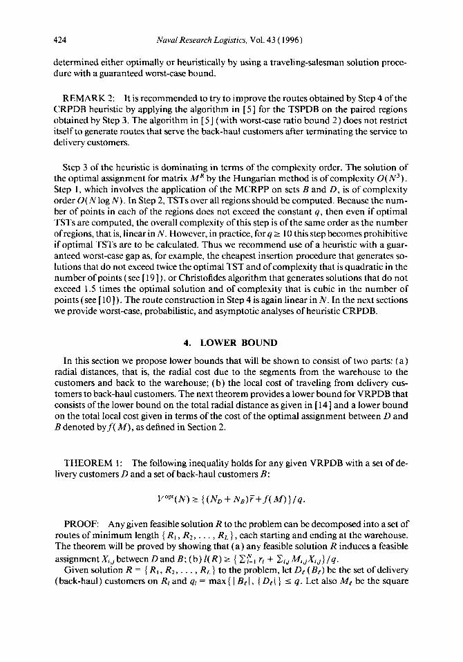
determined either optimally or heuristically by using a traveling-salesman solution procedure with a guaranteed worst-case bound.

REMARK 2: It is recommended to try to improve the routes obtained by Step 4 of the CRPDB heuristic by applying the algorithm in [ 51 for the TSPDB on the paired regions obtained by Step 3. The algorithm in [ 51 (with worst-case ratio bound 2) does not restrict itself to generate routes that serve the back-haul customers after terminating the service to delivery customers.

Step 3 of the heuristic is dominating in terms of the complexity order. The solution of the optimal assignment for matrix M R by the Hungarian method is of complexity O( N 3 ) . Step 1, which involves the application of the MCRPP on sets B and D, is of complexity order O( N log N ) . In Step 2, TSTs over all regions should be computed. Because the number of points in each of the regions does not exceed the constant q , then even if optimal TSTs are computed, the overall complexity of this step is of the same order as the number of regions, that is, linear in N . However, in practice, for q 2 10 this step becomes prohibitive if optimal TSTs are to be calculated. Thus we recommend use of a heuristic with a guaranteed worst-case gap as, for example, the cheapest insertion procedure that generates solutions that do not exceed twice the optimal TST and of complexity that is quadratic in the number of points (see [ 19]), or Christofides algorithm that generates solutions that do not exceed I .5 times the optimal solution and of complexity that is cubic in the number of points (see [lo]). The route construction in Step 4 is again linear in N . In the next sections we provide worst-case, probabilistic, and asymptotic analyses of heuristic CRPDB.

4. LOWER BOUND

In this section we propose lower bounds that will be shown to consist of two parts: ( a ) radial distances, that is, the radial cost due to the segments from the warehouse to the customers and back to the warehouse; (b) the local cost of traveling from delivery customers to back-haul customers. The next theorem provides a lower bound for VRPDB that consists of the lower bound on the total radial distance as given in [ 141 and a lower bound on the total local cost given in terms of the cost of the optimal assignment between D and B denoted by f ( M ) , as defined in Section 2.

THEOREM 1: The following inequality holds for any given VRPDB with a set of delivery customers D and a set of back-haul customers B :

V""'(N) L { ( N , + NB)Y+f( M ) } / q .

PROOF Any given feasible solution R to the problem can be decomposed into a set of routes of minimum length { R , , R2, . . . , RL} , each starting and ending at the warehouse. The theorem will be proved by showing that (a) any feasible solution R induces a feasible assignment Xi,, between Dand B ; (b) Z(R) 2 { 2zl ri + CijMi , jXi j } /q .

Given solution R = { RI , R2, . . . , RL} to the problem, let De ( B e ) be the set of delivery (back-haul) customers on Rl and ql = max { 1 Be 1, I Dt 1 I q . Let also Me be the square


matrix associated with the assignment problem between the sets De and Be as defined in Section 2. We will show that inequality (2) below holds for C = 1, . . . , L:

We first prove (2) for routes that consist of delivery (back-haul) customers only, and thus contain at most q customers: In that case note that because the assignment problem between De and Be assigns all customers to dummy customers at the origin, the right-hand side (RHS) of ( 2 ) equals 2 C R ~ r j / q t , which is twice the average radial distance of the customers on the route. This expression is clearly a lower bound on the length of the route. We prove now ( 2 ) for a feasible route Re consisting of k delivery customers and m back- haul customers, 1 I k s m I q and thus q p = m (the case m < k is an analogue): Number the delivery (back-haul ) customers clockwise from the warehouse according to the order of their occurrence on the route by 1 D, 2 O , . . . , k D ( 1 B , 2’, . . . , mB). Proving ( 2 ) is equivalent to proving that there exists a solution to the assignment problem between the sets Dp and Be such that the length of qe = m copies of route Re is not smaller than the cost of that assignment plus the sum of the radial distances of all customers on the route. The proof is by construction of such an assignment. Start with q p = m copies of route Re. Scan the route clockwise starting at the warehouse: Find the first arc on the route that connects two customers one from De and the other from Be. Assign these two customers one to the other. By using the triangle inequality it is easily observed that the length of one copy of Re is at least as large as the sum of the radial distances of these two customers plus the length of the arc connecting them. Mark these two specific customers and delete one copy of the route Re. We can repeat this step for k - 1 additional times, each time scanning the route as explained, searching for the first two unmarked customers of different types that are either connected by an arc or separated by marked customers only. Let these two customers be iD andjB 1 I i I k and 1 ~j I m and assign them one to the other. Delete one copy of route Re: The length of Re is at least as large as the sum of the radial distances to the customers iD and j B plus the length of the arc connecting them, which is the respective assignment cost. Terminate this iteration by marking these two customers. At the end of this procedure we are left with m - k 2 0 copies of Re and m - k unmarked back-haul customers. If rn - k > 0 then assign the unmarked back-haul customers to the dummy delivery customers at the origin at a cost of their radial distances. Note that each copy of Re is at least as large as twice the radial distance to any of the customers. Thus the length of the rn - k left copies of Re is at least as large as twice the sum of the radial distances of the unmarked back-haul customers, resulting in ( 2 ) . Substituting q p by q in ( 2 ) preserves the inequality, because q p I q . Therefore we conclude, in view of the proposed procedure, and by summing ( 2 ) over all the routes C = 1, . . . , L , that according to solution R there exist two sets of marked customers of the same cardinality, one a subset of B and the other a subset of D, and two sets of unmarked customers, one a subset of B and the other a subset of D. The length of q copies of the solution is shown above to be at least as large as the optimal assignment between the two sets of marked customers plus the sum of the radial distances of all marked customers plus twice the radial distance of all unmarked customers. In order to terminate the proof it is sufficient to show that there exists an assignment between the unmarked delivery customers and the unmarked back-haul customers whose cost is bounded from above by the sum of the radial distances to all unmarked customers.


Indeed, we show that any assignment between the two sets of unmarked customers satisfies the above inequality, because the sum of the radial distance to two unmarked customers is at least as large as the length of the arc connecting them. Therefore, the sum of the radial distances to all unmarked customers is bounded from below by the cost of any feasible assignment to problem ( 1 ) when applied on the two sets of unmarked customers. 0

In the remainder of this section we use the lower bound of Theorem 1 to develop an alternative lower bound that does not require the computation of f( M ) and instead is given in terms of the optimal assignment costf( M R ) , which we compute in the heuristic process. We first evaluate the gap between the optimal cost of the assignment between the sets D and B on one hand, and D* and B* on the other hand. According to Section 3 the optimal cost of assignment problem ( 1 ) between the sets D* and B* is denotedf( M*).

CLAIM 1: The following inequality holds when solving assignment problem ( 1 ) on the distance matrices M and M*:

PROOF Note that both matrices M a n d M* are square matrices. According to the assumption that No 2 NB, matrix M is of size N i and contains A( M ) = No - NB columns of dummy back-haul customers. Matrix M* is of size N ; *, where

ND - q,

qLND/qJ, otherwise.

if No is an integer multiple of q but NB is not, ND* =

Matrix M* is obtained from matrix Mby omitting No - ND* I q rows ofdelivery customers and NB - qLNB/qJ I q - 1 columns of back-haul customers and either adding or deleting dummy back-haul customers in order to have exactly N D * columns. Matrix M* contains A(M*) = ND= - qLNB/qJ dummy back-haul customers at the origin.

We will construct a feasible solution to the assignment problem between D* and B* by modifying an optimal assignment solution between the sets D and B. Let { X l , J } i E 0,; E B U B‘ be an optimal solution to problem ( 1 ) between D and B with costf( M ) . Let { Yl,,} 1 I i , j I ND* be a solution to assignment problem ( 1 ) between D* and B*. Let also B*’ denotes the set of dummy back-haul customers in the second problem. We call B* (D*) the undeleted columns (rows) of B (D), respectively. We distinguish between two cases: (a) A( M * ) I A( M ) ; ( b ) A( M * ) > A( M ) . In the first case the set B*’is a subset of undeleted columns of the set of dummy back-haul customers B‘, and in the second case the set B*‘ includes the set B’ that is a set of undeleted columns of Mand contains in addition I B*‘l - I B’I new dummy back-haul customers. We explain below how to construct an assignment { Y,,,) from D* to B* U B*’ given { X l , , } .

Suppose Xl,J = I . If i is an undeleted row and j is an undeleted column then let Y,,, = 1 ; that is, keep the arc between i andj; if i is a deleted row a n d j is a deleted column omit the arc between i and j as well as the two nodes i andj ; if i is a deleted ( undeleted) row a n d j is an undeleted (deleted) column then mark nodej ( i ) and omit the arc connecting i to; as well as node i (j). In case (b) add I B*’l - I B* I new dummy back-haul nodes and mark them. At the end of the process we are left with a subassignment { Yl,,} of { X,,,} and with equal cardinality sets of marked delivery customers and marked back-haul customers. We


note that in case (a) the set of marked back-haul customers is included in B U B', and therefore the number of marked back-haul customers is at most as the number of deleted delivery customers, that is, at most q . In case (b) no columns are deleted from B', thus the number of marked delivery customers is at most as the number of deleted columns from B , i.e., at most q - 1. Thus in either case the number of marked customers of each type is bounded by q . In order to complete assignment { Y i j } , i E D*, j E B* U B*', we define a subassignment problem from the marked delivery customers to the marked back-haul customers. Because the cost of each arc in this assignment problem is bounded from above by 2R and there are at most q arcs in any such subassignment, the cost of the obtained subassignment is bounded from above by 2qR. We conclude that

In order to derive a lower bound in terms off( M") we define matrix M* * to be of the same dimension as matrix M* such that for delivery customer i that belongs to region De and back-haul customerj that belongs to region &, M t y = min ( d ( t , s): t E Dl and s E Bk 1. I f j is a dummy customer then is the minimum radial distance over all customers in Dp. The rows (columns) of M** can be partitioned into sets of q identical rows (columns), because any two rows (columns) of the same region are identical and all regions are assumed to consist of exactly q customers. The matrix M** is componentwise bounded from above by the matrix M*. Therefore,

f( M**) If( M*). ( 3 )

Matrix M" as defined in Section 3 is indeed obtained by taking one representative row and one representative column from any group of q rows/columns of M** that is associated with a delivery/ back-haul region. The next claim establishes the relationship between f( M**) andf( M").

CLAIM 2: There exists an optimal assignment solution for M** that consists of q copies of any given optimal assignment solution to M": One of the optimal assignments to M* * assigns all q customers in any delivery region D, to the q customers in back-haul region Bk, where D, is assigned to Bk in the given optimal assignment to M". In particular,f( M") = f( M* * )/ 4 .

PROOF The assignment problem formulation corresponding to the matrix M" is as follows:

s.t. C Xp,k = 1,

&,k = 1 ,

Xe,k E { 0, 1 },

for all back-haul regions Bk,

for all delivery regions Dp,

for all C and k.

e

k

(4)


Because of the special structure of the matrix M* *, where each of the rows and columns has exactly q copies identical to a row (column ) of matrix M R and the cost of assigning any copy of row i E Dp to any copy of column j , j E Bk, is M&, the assignment problem corresponding to M* * can be written in terms of (4) by multiplying the RHS vector of the constraints by q and allowing the variables to assume values in { 0, 1,2, . . . , q } . Thus Xp,k = q’, where q’ I q means that q’ copies of the rows corresponding to region Dp are assigned to q’ copies of the columns corresponding to region Bk. Because this formulation is obtained from (4) by multiplying the RHS vector by the constant q , then according to linear programming theory multiplying the optimal assignment to (4) by q is an optimal solution tof( M**). Thus,f( M**) = qf( M R ) . 0

Based on Theorem 1, Claims 1 and 2, and inequality ( 3 ) we obtain the following lower bound for the optimal cost.

THEOREM 2: Given is a VRPDB with sets of delivery customers D and back-haul customers B. If the MCRPP is applied separately on D and B and the matrix M R is con- structed accordingly, then

VoP*( N ) 2 ( ND + NB)F/q + max { 0, f( M R ) - 2 R 1.

REMARK: The lower bound given in Theorem 2 is not as tight as the one given in Theo- rem 1. However, as will be shown, it is also asymptotic optimal. Its advantages are (a) it requires solving an assignment problem on matrix M R whose dimension is 1 / q of the dimension of M ; (b) the solution off( M R ) is required anyway when applying heuristic CRPDB.

In the next section we bound from above the cost generated by applying the CRPDB heuristic and we discuss the modifications required for general delivery/ back-haul sizes.

5. UPPER BOUND ON VcRPDB

Let TSP(X) be the length of the optimal TST via the customers in a set X , and TSP“( X ) be the length of a TST via X obtained by a heuristic with a worst-case bound of 1 + a. According to the procedure used to solve the TSTs we denote the proposed heuristic by CRPDB (aCRPDB) if optimal (( 1 + a ) - optimal) TSTs are calculated in each region

denote the respective cost of heuristic CRPDB (aCRPDB). The following theorem provides an upper bound on the cost of the proposed heuristic.

( note that heuristic OCRPDB coincides with CRPDB). Also let, VCRPDB( A’) ( VaCRPDB ( N ) )

THEOREM 3: The following inequality holds when applying heuristic aCRPDB for any a 2 0:

PROOF In order to prove the inequality we distinguish between vehicles that serve both delivery and back-haul customers and vehicles that serve a single type of customer.


(a) Suppose that according to assignment 2 (see Step 3 of CRPDB heuristic), Dp is assigned to B k , C I rND/q1 and k I rNB/ql at the cost d(s , t) with C p , k

= (s, t). Also suppose that a E Dp ( b E Bk) is a customer with minimum radial distance in Dp (Bk). According to the proposed heuristic the total length of the route of this vehicle is bounded from above by r, + TSPa( De) + d(a, s) + d(s, t ) + TSPa(Bkj + d ( t , b ) + rb. In view ofthe triangle inequality d(a, s) I TSP(Dp)/2 and d ( t , b) I TSP(Bk)/2. IfDp c D* and B k

E B* then De and Bk are assigned one to the other at the cost of d(s, 2) according tof( M R ) . Otherwise, that is, C = L O and k = L B , d( s, t ) I 2 R.

(b) If D, (&) is served by a separate vehicle, then according tof( M R ) the assignment cost due to Dp (&) is r,, where a is a customer with the minimal radial distance in the region. According to the heuristic the length ofthe route ofthat vehicle is bounded from above by 2r, + TSPa( 4) ( 2ra + TSPn( Bk)) ,

where region Dp (&) is assigned to a dummy region at the cost of r, according to f ( M R ) . Therefore, VaCRPDB(N) I CI [ min { ri : i E DI } + TSPa( D,) + O.STSP( D p ) ] + c k [ min { ri : i E Bk} + TSP"( Bk) + O.STSP( Bk)] +f( M R ) + 2R 5 C$erl ED, r i / q + C ~ E ; ' CB, r i / q + 2R + (1.5 + a) ( C p TSP(Dp)

2R I (No 4- N B ) q q + (1.5 + a ) ( c p TSP(Dp) + C k TSP(Bk)) +f( hifR) + 4R.

C k TSP(Bk)) +f( M R )

The second inequality follows from the following facts:

1. Delivery (back-haul) regions 1, . . . , L D - 1 ( 1, . . . , L B - 1 ) consist of exactly q customers; thus the minimal radial distance in that region is bounded from above by the average of the radial distances in the region.

2. For regions DLD and BLs we bound the minimal radial distance by R . The last inequality is straightforward. 0

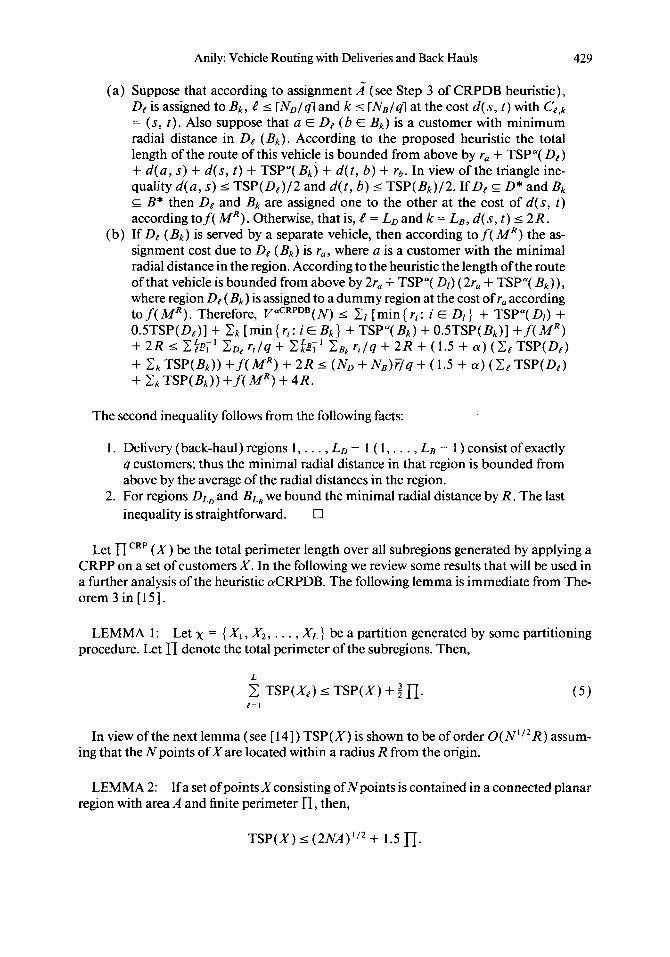
Let n CRP (X) be the total perimeter length over all subregions generated by applying a CRPP on a set of customers X. In the following we review some results that will be used in a further analysis of the heuristic aCRPDB. The following lemma is immediate from The- orem 3 in [15] .

LEMMA 1 : Let x = {XI, X 2 , . . . , X L } be a partition generated by some partitioning procedure. Let n denote the total perimeter of the subregions. Then,

L

2 TSP(Xp) I TSP(X) + 3 I'I. e= I

In view of the next lemma (see [ 141) TSP(X) is shown to be of order O(N1l2R) assuming that the Npoints ofXare located within a radius R from the origin.

LEMMA 2: Ifa set ofpointsXconsisting ofNpoints is contained in a connected planar region with area A and finite perimeter n, then,

TSP(X) I (2NA)'12+ 1.5 n.


The next lemma, also given in [ 141, demonstrates that the second term on the RHS of (5 ) is of order O( N 1 / 2 R ) as well, if a CRPP is applied.

LEMMA 3: If the CRPP is applied [with q points in all regions (except possibly one)] on a set of points Xconsisting of n points and ri the radial distance of point i, then

The next theorem combines the results of Theorem 3 and the three lemmas and provides an upper bound on the cost of heuristic aCRPDB in terms of the average radial distance of all customers, the number of customers N , q , R , and the optimal assignment costf( M R ) :

THEOREM 4: Given are ( a ) a set of N back-haul and delivery customers dispersed within a radius R of the warehouse, each having a requirement size of one unit and (b) a fleet of identical vehicles with capacity q. Then, the cost generated by applying heuristic aCRPDB is bounded by

v aCRPDB ( N ) I ( N o + Ns)F//q + f ( M R ) + ( 2 ~ ) ’ / * ( 1.5 + a)R(ND + NB)’/’

X [ l + 1.5(3/q)”*] + ( 1 3 . 5 ~ + 17.5 + 947r + 1))R.

PROOF Note that according to Lemmas 1-3,

LD LB

2 TSP(D1) + 2 TSP(Bk) I TSP(N) + 1.5 n c R p ( D ) + n CRP(B) 5 (2Nn)’”R + 3nR I= I k= 1

+ ( 6 + 47r)R I (2Nn)I l2R + 3nR 1 + 1.5(6nR/q)I/’( i e N r i ) 1 / 2 + ( 9 + 6 n ) R .

The last inequality follows from the fact that the square root is a concave function and as such it obtains its maximum when CiEo ri = C i E B ri . The desired inequality directly follows from Theorem 3 and the above inequality. 0

The lower and upper bounds presented above continue to hold also if not all delivery and back-haul sizes are one unit. In the general case, delivery (back-haul) customer i can be viewed as di ( bi ) delivery (back-haul) points each with requirement size of one unit and all located at the customer’s location; see also [ 141. The generalization to general requirement sizes enables us to solve also the multicommodity case: Let the vehicle’s capacity as well as the requirement sizes of the customers to be specified in terms of weight. The unit weight may be scaled so that the vehicle’s capacity and all requirement sizes are approxi- mately integers. Assuming that the vehicle may carry any mixture of commodities, the CRPDB heuristic for general requirement sizes may be applied.

For the single-commodity and general requirement sizes or for the multicommodity case, we let Fbe defined as the weighted average radial distance with weights proportional

Anily: Vehicle Routing with Deliveries and Back Hauls 43 1

to the customers' requirements; see Section 2. The assignment problems used in the lower and upper bounds should be defined on the sets of delivery and back-haulpoints. However, if we do not assume that the requirement sizes are bounded, then the matrices corresponding to the assignment problems on the set of points might be of unbounded size in N , resulting in a nonpolynomial algorithm. We present below an alternative scheme for these cases, which instead of solving assignment problems, solves a transportation (Hitchcock) problem on the set of customers. The modifications required in the application of CRPDB heuristic are as follows: In Step I of the heuristic MCRPP is applied on the set of delivery and back-haul points separately such that the plane is partitioned into a number of regions, all consisting of q points, except one region of each type, which may contain less than q points. Observe that if the delivery (back-haul) size of customer i is greater than q , that is, it equals kl ,q + k2i , k , , 2 1, and 0 I k,, I q - 1, then it is sufficient to apply MCRPP in Step 1 of CRPDB on k2i delivery (back-haul) points located at customer i's location and add to the list of regions generated by MCRPP k l i delivery (back- haul) regions consisting of q points all located at customer i's location. Thus, independently of the order of the delivery and back-haul sizes, Step 1 is of complexity O( N log N). Obvi- ously, Step 2, which requires computing the TSTs in the regions, is linear in I NI , because no additional work is required for the above k l i regions. Step 3 requires the solution of an assignment problem defined on all generated regions. The dimension of the corresponding matrix M R depends on the customers' delivery/back-haul sizes. As mentioned above, f( M R ) may be computed as a transportation (Hitchcock) problem (see [ 18, Chap. 71): the kli delivery (back-haul) regions associated with customer i , each consisting of q points of customer i , may be presented as a single delivery (back-haul) zone with delivery (back- haul) requirement of k l i units. A region that consists of points from more than one customer is a zone by itself with requirement size of one unit. It is easy to see that the number of delivery (back-haul) zones is bounded from above by 2 ID I (2 I B I ). If the total requirement of the delivery zones is greater (smaller) than the total requirement of the back- haul zones, then a single dummy back-haul (delivery) zone is added such that its total requirement size is the difference between the total requirement size of the zones from the two types. The matrix of distances between the delivery and back-haul zones is computed. The obtained matrix is not necessarily a square one. The transportation problem is defined similarly to problem ( l ) , where the right-hand side of the constraint associated with a certain zone equals its requirement size. Because the constraint matrix is total unimodal we can relax the last set of constraints to X,,, 2 0. X l j = k means that k regions in delivery zone i are assigned to k regions in back-haul zonej. This problem can be solved efficiently by linear programming software. However, in terms of complexity, the problem can be viewed as a minimum cost flow problem with O ( N ) nodes and O ( N 2 ) uncapacitated arcs. The best known strong polynomial for the transportation problem as defined above is of complexity O( N 3 log N) , and is presented in [ 17 1. We note that for this complexity bound we do not need to assume that the requirement sizes are bounded. However, if all requirement sizes are uniformly bounded by a constant independent of N , then solving as an assignment problem on the set of points requires O( N 3 ) operations.

In the next section we provide a guaranteed worst-case gap and probabilistic and asymptotic analyses of heuristic aCRPDB.

6. ANALYSIS OF KRPDB HEURISTIC The next theorem provides a relative error bound for aCRPDB heuristic: THEOREM 5: Given is a fleet of identical vehicles of capacity q , a set of N delivery


and back-haul customers dispersed within a radius R from the warehouse, with a total delivery size of No and a total back-haul size of NB. Then, the following worst-case gap holds for aCRPDB heuristic:

PROOF The proof is immediate in view of Theorems 2 and 4 and the above discussion 0 regarding general delivery and back-haul sizes.

The relative error bound given in Theorem 5 holds also for the special case that all customers are of a single type and is of a similar order to the one given in [ 141. Note that in this special c a f ( M) = M, so the lower bound in Theorem 1 coincides with that in [ 141.

THEOREM 6: Let Y ( n ) = {yl , y2 , . . . , y,,} be a random set of n customers each characterized by its radial distance r; , an indicator Z; that assumes the value + 1 ( - 1 ) if the customer is a delivery (back-haul) customer, its requirement size pi and its polar coordi- nate. The pairs ( ri , p; ) are assumed to be i.i.d. and pi is a discrete random variable assuming positive integer values, which is independent of r, . Let [ = E( r; ) and p = E( 1; ) be finite.

(a) limn+m inf( l /n )VoP' (Y(n) )2p[ /q . (b) If, in addition, [ > 0 and p > 0 and the random variables rj are uniformly

bounded from above by the constant R < co , then

lim ( vaCRPDB ( Y ( n ) ) - vop'(Y(n)))/Vopt(Y(n)) = 0, a s n-m

PROOF This part follows from Theorem 1 , the fact that p j is independent of ri , and the law of large numbers. In view of part ( a ) , the assumption that p > 0 and 4 > 0, it suffices to show that

lim ( vaCRPDB ( Y ( n ) ) - Vopt( Y( n ) ) ) / n = 0, a.s. n-m

According to Theorems 2 and 4:

0 I vaCRPDB ( Y ( n ) ) - Vop'(Y(n)) 5 ( 2 r ) ' l 2 ( 1.5 + &)R [ l + 1 .5 (3 /q )1 /2 ]

+ ( 1 3 . 5 ~ + 19.5 + 9 a ( ~ + 1) )R .

According to the rule of large numbers limn-m( C p j ) ' 1 2 / n = limn+m \111/ fi = 0; thus

lim ( vaCRPDB ( Y ( n ) ) - Vopt( Y ( n ) ) ) / n = 0, a s . n- m

The proof of Theorem 6 gives us also the convergence rate of (VaCRPDB ( Y ( n ) ) -


Vop’( Y ( n ) ) ) / n to zero, which is of order 1 / fi. According to the theorem we see that we assume extremely mild conditions on the distribution of p, that may be unbounded, but we need to ensure that its expectation is finite. As mentioned in [ 31, the assumption that the pairs ( r, , pi ) are i.i.d. and that w, is independent of r, is needed only to assure that the lower bound grows linearly in n almost surely. The assumption is needed to preclude heavy concentration of points with small p l r j values. Similarly, the condition that the radial distances are uniformly bounded from above is unnecessarily strong. One merely needs that max { r, : 1 I i I n } does not grow too fast as IZ + 00 (as.). Much simpler conditions with respect to the distribution of r, may be invoked; see [ 1 1 1.

REFERENCES

[ 1 ] Anily, S., “The General Multi-Retailer EOQ Problem with Vehicle Routing Costs,” European Journal of Operations Research, 79,69-9 1 ( 1994).

[ 21 Anily, S., and Federgruen, A., “One Warehouse Multiple Retailer Inventory Systems with Ve- hicle Routing Costs,” Management Science, 36,92- 1 14 ( 1990).

[ 31 Anily, S., and Federgruen, A., “A Class of Euclidean Routing Problems with General Route Costs Functions,” Mathe~atjcs of Operations Research, 15,268-285 ( 1990).

[ 41 Anily, S., and Federgruen, A., “Two-Echelon Distribution Systems with Vehicle Routing and Central Inventories,” Special Issue on Stochastic and Dynamic Models in Transportation, ed- ited by M. Dror, Operalions Research, 41, 37-47 ( 1993).

[ 51 Anily, S., and Mosheiov, G., “The Traveling Salesman Problem with Delivery and Backhauls,” Operations Research Letters, 16, 1 1 - 18 ( 1994).

[ 61 Arkin, E.M., Hassin, R., and Mein, L., “Restricted Delivery Problems on a Network,” Working Paper, Department of Statistics and Operations Research, School of Mathematical Sciences, Tel-Aviv University, Tel-Aviv 69978, Israel, 1995.

[ 71 Bodin, L., Golden, B.L., Assad, A., and Ball, M., “Routing and Scheduling of Vehicles and Crews-State of the Art,” Computers and Operations Research, 10,63-2 I I ( 1983).

[ 81 Burns, L.D., Hall, R.W., Blumenfeld, D.E., and Daganzo, C.F., “Distribution Strategies that Minimize Transportation and Inventory Costs,” Operations Research, 33,469-490 ( 1985).

[ 91 Casco, D.O., Golden, B.L., and Wasil, E.A., “Vehicle Routing with Backhauls: Models, Algo- rithms, and Case Studies,” in B.L. Golden and A.A. Assad (Eds.), Studies in Management Science and Systems/ Vehicle Routing: Methods and Studies, North Holland, Amsterdam,

[ 101 Christofides, N., “Worst-Case Analysis of a New Heuristic for the Traveling Salesman Prob-

[ 1 1 ] David, H. A., Order Statistics, Wiley, New York, 1970. [ 121 Federgruen, A., and Simchi-Levi, D., “Analytical Analysis of Vehicle Routing and Inventory-

Routing Problems,” ( 1992) to be published in M. Ball, T. Magnanti, C . Monma, and G. Nem- hauser ( Eds.), Handbooks in Operations Research and Management Science, volume on Net- works and Distribution, in press.

[ 131 Garey, M.R., and Johnson, D.S., Computers and Intractability: A Guide to the Theory of NP Completeness, Freeman, San Francisco, 1979.

[ 141 Haimovich, M., and Rinnooy Kan, A.H.G., “Bounds and Heuristics for Capacitated Routing Problems,” Mathematics of Operations Research, 10,527-542 ( 1985).

[ 151 Karp, R.M., “Probabilistic Analysis of Partitioning Algorithms for the Traveling Salesman Problem in the Plane,” Mathematics of Operations Research, 2,209-244 ( 1977).

[ 161 Mosheiov, G., “The Traveling Salesman Problem with Pick-Up and Delivery,” Working Paper, School of Business Administration and the Statistics Department, The Hebrew University, Jerusalem, Israel, I99 1,

[ 171 Orlin, J.B., “A Faster Strongly Polynomial Minimum Cost Flow Algorithm,” Operations Re- search, 41,338-350 (1993).

1988, pp. 127-147.

lem,” Technical Report, GSIA, Carnegie-Mellon University, 1976.


[ 181 Papadimitriou, C.H., and Steiglitz, K., Combinarorial Optimization Algorithms and Complex-

[ 191 Rosenkrantz, D.J., Steams, R.E., and Lewis, P.M., “An Analysis of Several Heuristics for the

[ 201 Schneider, L.M., “New Era in Transportation Strategy,” Transportation Strategy, 1 18- 126

ity, Prentice Hall, Inc., Englewood Cliffs, NJ, 1982.

Traveling Salesman Problem,” SZAMJournal on Computing, 6,563-58 1 ( 1977).

(1985).

Manuscript received April 1994 Revised manuscript received June 1995 Accepted September 23, 1995

the vehicle-routing problem with delivery and back-haul …anily/publications/16.pdf · ·...

Documents