the visual recognition machine jitendra malik university of california at berkeley jitendra malik...

The Visual Recognition MachineThe Visual Recognition Machine

Jitendra Malik

University of California at Berkeley

Jitendra Malik

University of California at Berkeley

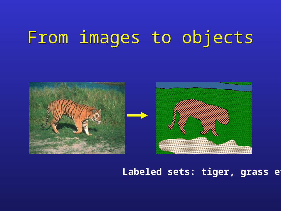
From images to objectsFrom images to objects

Labeled sets: tiger, grass etc

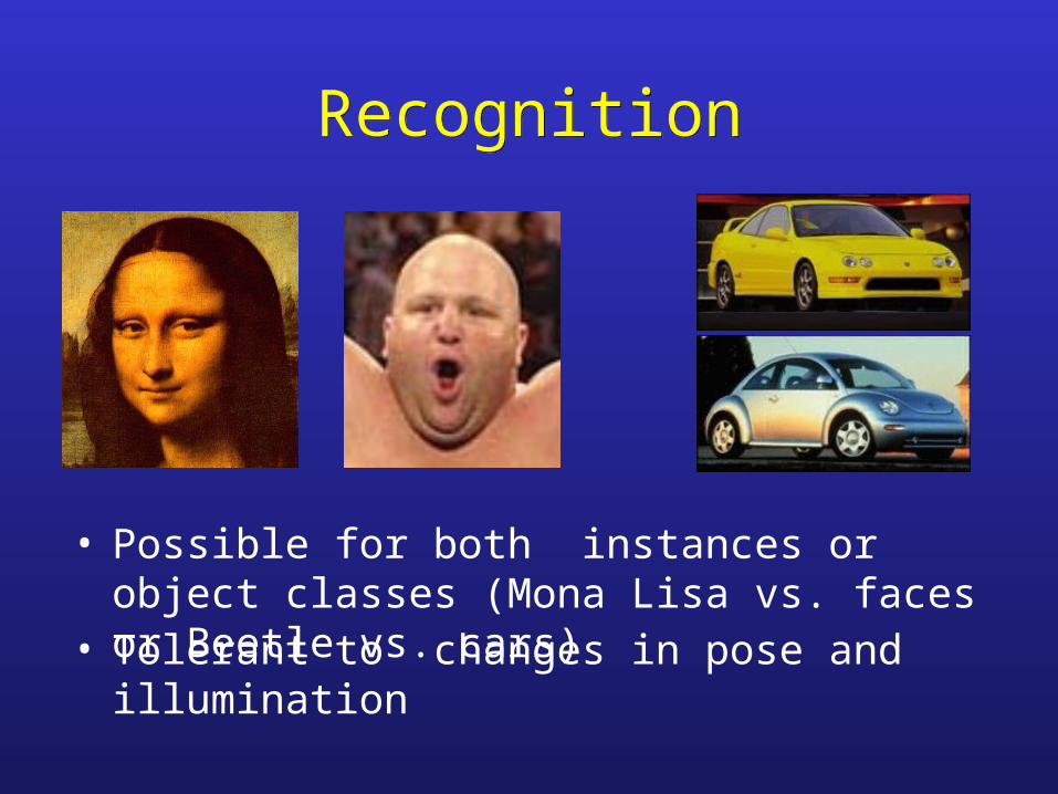
RecognitionRecognition

• Possible for both instances or object classes (Mona Lisa vs. faces or Beetle vs. cars)

• Tolerant to changes in pose and illumination

Three stagesThree stages

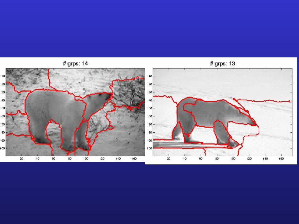
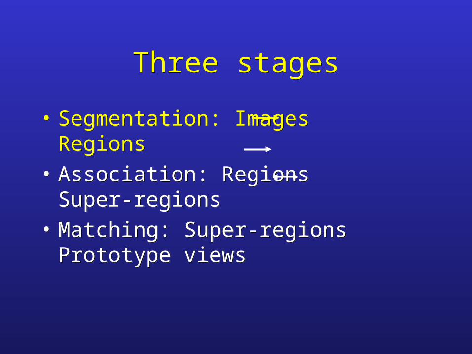
• Segmentation: Images Regions

• Association: Regions Super-regions

• Matching: Super-regions Prototype views




Boundaries of image regions defined by a number of attributes

Boundaries of image regions defined by a number of attributes

– Brightness/color

– Texture

– Motion

– Stereoscopic depth

– Familiar configuration

– Brightness/color

– Texture

– Motion

– Stereoscopic depth

– Familiar configuration

Image Segmentation as Graph PartitioningImage Segmentation as Graph PartitioningBuild a weighted graph G=(V,E) from image

V: image pixels

E: connections between pairs of nearby pixels

region

same the tobelong

j& iy that probabilit :ijW

Partition graph so that similarity within group is large and similarity between groups is small -- Normalized Cuts [Shi&Malik 97]

Some Terminology for Graph Partitioning

Some Terminology for Graph Partitioning

• How do we bipartition a graph:• How do we bipartition a graph:

BAwith

BA,

),,W(B)A,(vu

vucut

disjointy necessarilnot A' andA

A'A,

),(W)A'A,(

vu

vuassoc

Normalized Cut, A measure of dissimilarity

Normalized Cut, A measure of dissimilarity

• Minimum cut is not appropriate since it favors cutting small pieces.

• Normalized Cut, Ncut:

• Minimum cut is not appropriate since it favors cutting small pieces.

• Normalized Cut, Ncut:

V),(

B)A,(

V)A,(

B)A,( B)A,(

Bassoc

cut

assoc

cutNcut

Solving the Normalized Cut problem

Solving the Normalized Cut problem

• Exact discrete solution to Ncut is NP-complete even on regular grid,– [Papadimitriou’97]

• Drawing on spectral graph theory, good approximation can be obtained by solving a generalized eigenvalue problem.

• Exact discrete solution to Ncut is NP-complete even on regular grid,– [Papadimitriou’97]

• Drawing on spectral graph theory, good approximation can be obtained by solving a generalized eigenvalue problem.

Normalized Cut As Generalized Eigenvalue problem

Normalized Cut As Generalized Eigenvalue problem

• after simplification, we get• after simplification, we get

...

),(

),( ;

11)1(

)1)(()1(

11

)1)(()1(

)VB,(

)BA,(

)VA,(

B)A,(B)A,(

0

i

x

T

T

T

T

iiD

iiDk

Dk

xWDx

Dk

xWDx

assoc

cut

assoc

cutNcut

i

.01},,1{ with ,)(

),(

DybyDyy

yWDyBANcut T

iT

T

Computational AspectsComputational Aspects

• Solving for the generalized eigensystem:

• (D-W) is of size , but it is sparse with O(N) nonzero entries, where N is the number of pixels.

• Using Lanczos algorithm.

• Solving for the generalized eigensystem:

• (D-W) is of size , but it is sparse with O(N) nonzero entries, where N is the number of pixels.

• Using Lanczos algorithm.

.D where,W)D-D(D

DW)-(D

2

1

2

1-

2

1-

xzzz

xx

NN

AssociationAssociation

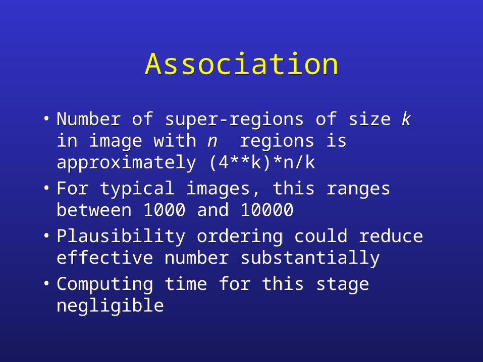
• Number of super-regions of size k in image with n regions is approximately (4**k)*n/k

• For typical images, this ranges between 1000 and 10000

• Plausibility ordering could reduce effective number substantially

• Computing time for this stage negligible

• Number of super-regions of size k in image with n regions is approximately (4**k)*n/k

• For typical images, this ranges between 1000 and 10000

• Plausibility ordering could reduce effective number substantially

• Computing time for this stage negligible

Matching Matching

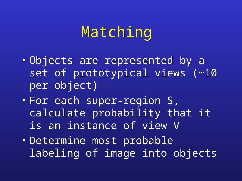
• Objects are represented by a set of prototypical views (~10 per object)

• For each super-region S, calculate probability that it is an instance of view V

• Determine most probable labeling of image into objects

• Objects are represented by a set of prototypical views (~10 per object)

• For each super-region S, calculate probability that it is an instance of view V

• Determine most probable labeling of image into objects

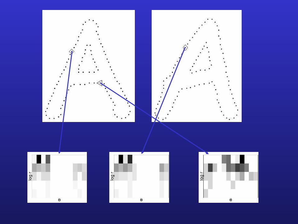
Matching super-regions to viewsMatching super-regions to views

• Based on color, texture and shape similarity• Color, texture matching is relatively well

understood and fast• Shape matching is difficult because the

algorithm should tolerate pose, illumination and intra-category variation

• GOAL: small misclassification error with few views.

• Based on color, texture and shape similarity• Color, texture matching is relatively well

understood and fast• Shape matching is difficult because the

algorithm should tolerate pose, illumination and intra-category variation

• GOAL: small misclassification error with few views.

Core ideaCore idea

• Find corresponding points on the two shapes and use those to deform prototype into alignment

• Allowing this flexibility reduces number of prototype views needed

• Find corresponding points on the two shapes and use those to deform prototype into alignment

• Allowing this flexibility reduces number of prototype views needed

MNIST Handwritten Digits

Digit Prototypes

Matching with original and deformed prototypesPrototype Test Error

Deforming prototypes using thin plate splines

Only 25 deformable templates needed (instead of 60 K) to get 5% error

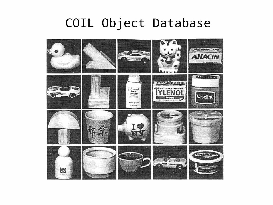
COIL Object Database

Computing cost on a Pentium PCComputing cost on a Pentium PC

• Segmentation: 5 minutes /image

• Matching : 0.5 sec / match

• Segmentation: 5 minutes /image

• Matching : 0.5 sec / match

Cost on 10**4 node machine Cost on 10**4 node machine

• Segmentation: 0.03 sec /image, which is 30 Hz (video rate)

• Matching : 20K matches/sec at full resolution (100 points/shape)

• Segmentation: 0.03 sec /image, which is 30 Hz (video rate)

• Matching : 20K matches/sec at full resolution (100 points/shape)

How many prototype views can one match at 1 Hz?

How many prototype views can one match at 1 Hz?

• 1K candidate super-regions• Consider only 1% of matches at full

resolution (10% pass color/texture filter, 10% of those pass low resolution shape filter)

• If half time spent in pruning and half in full resolution matching, 1000 prototype views can be matched at 1 Hz.

• 1K candidate super-regions• Consider only 1% of matches at full

resolution (10% pass color/texture filter, 10% of those pass low resolution shape filter)

• If half time spent in pruning and half in full resolution matching, 1000 prototype views can be matched at 1 Hz.

What can one do with matching 1000 views a second?

What can one do with matching 1000 views a second?

• Worst case: 100 object categories

• Best case depends on how well one can exploit context, hierarchy and hashing.

• Cf. humans can recognize 10-100K objects

• Worst case: 100 object categories

• Best case depends on how well one can exploit context, hierarchy and hashing.

• Cf. humans can recognize 10-100K objects

Memory requirementsMemory requirements

• 10 K object categories * 10 views/category * 100 * 100 pixels/view * 1 byte/pixel gives us 1 Gigabyte.

• 10 K object categories * 10 views/category * 100 * 100 pixels/view * 1 byte/pixel gives us 1 Gigabyte.

Concluding remarks Concluding remarks

• Speech in 1985 was in the same state as vision in 2000. Hidden Markov Models adoption led to a decade of research which refined the paradigm for continuous speech recognition.

• The proposed 3 stage framework for recognition: segmentation, association and matching, could provide the same focus and coherence to vision research leading to general purpose object recognition in 10 years.

• Speech in 1985 was in the same state as vision in 2000. Hidden Markov Models adoption led to a decade of research which refined the paradigm for continuous speech recognition.

• The proposed 3 stage framework for recognition: segmentation, association and matching, could provide the same focus and coherence to vision research leading to general purpose object recognition in 10 years.

the visual recognition machine jitendra malik university of california at berkeley jitendra malik...

Documents

regions superregions

n regions

images regions association

boundaries of image

views slide

berkeley slide

illumination slide

views segmentation