the wavescalar architecturecseweb.ucsd.edu/~swanson/papers/swansonphdthesis.pdfthe wavescalar...
TRANSCRIPT
The WaveScalar Architecture
Steven Swanson
A dissertation submitted in partial fulfillmentof the requirements for the degree of
Doctor of Philosophy
University of Washington
2006
Program Authorized to O↵er Degree: Computer Science & Engineering


University of WashingtonGraduate School
This is to certify that I have examined this copy of a doctoral dissertation by
Steven Swanson
and have found that it is complete and satisfactory in all respects,and that any and all revisions required by the final
examining committee have been made.
Chair of the Supervisory Committee:
Mark Oskin
Reading Committee:
Mark Oskin
Susan Eggers
John Wawrzynek
Date:

In presenting this dissertation in partial fulfillment of the requirements for the doctoraldegree at the University of Washington, I agree that the Library shall make itscopies freely available for inspection. I further agree that extensive copying of thisdissertation is allowable only for scholarly purposes, consistent with “fair use” asprescribed in the U.S. Copyright Law. Requests for copying or reproduction of thisdissertation may be referred to Proquest Information and Learning, 300 North ZeebRoad, Ann Arbor, MI 48106-1346, 1-800-521-0600, or to the author.
Signature
Date


University of Washington
Abstract
The WaveScalar Architecture
Steven Swanson
Chair of the Supervisory Committee:Assistant Professor Mark OskinComputer Science & Engineering
Silicon technology will continue to provide an exponential increase in the avail-
ability of raw transistors. E↵ectively translating this resource into application per-
formance, however, is an open challenge that conventional superscalar designs will
not be able to meet. We present WaveScalar as a scalable alternative to conven-
tional designs. WaveScalar is a dataflow instruction set and execution model de-
signed for scalable, low-complexity, high-performance processors. Unlike previous
dataflow machines, WaveScalar can e�ciently provide the sequential memory seman-
tics imperative languages require. To allow programmers to easily express parallelism,
WaveScalar supports pthread-style, coarse-grain multithreading and dataflow-style,
fine-grain threading. In addition, it permits blending the two styles within an appli-
cation or even a single function.
To execute WaveScalar programs, we have designed a scalable, tile-based processor
architecture called the WaveCache. As a program executes, the WaveCache maps the
program’s instructions onto its array of processing elements (PEs). The instructions
remain at their processing elements for many invocations, and as the working set
of instructions changes, the WaveCache removes unused instructions and maps new
instructions in their place. The instructions communicate directly with one-another
over a scalable, hierarchical on-chip interconnect, obviating the need for long wires

and broadcast communication.
This thesis presents the WaveScalar instruction set and evaluates a simulated
implementation based on current technology. For single-threaded applications, the
WaveCache achieves performance on par with conventional processors, but in less
area. For coarse-grain threaded applications, WaveCache performance scales with
chip size over a wide range, and it outperforms a range of the multi-threaded designs.
The WaveCache sustains 7-14 multiply-accumulates per cycle on fine-grain threaded
versions of well-known kernels. Finally, we apply both styles of threading to an
example application, equake from spec2000, and speed it up by 9⇥ compared to the
serial version.

TABLE OF CONTENTS
List of Figures . . . . . . . . . . . . . . . . . . . . . . . . . . . . . . . . . . . iii
List of Tables . . . . . . . . . . . . . . . . . . . . . . . . . . . . . . . . . . . . v
Chapter 1: Introduction . . . . . . . . . . . . . . . . . . . . . . . . . . . . 1
Chapter 2: WaveScalar Sans Memory . . . . . . . . . . . . . . . . . . . . . 5
2.1 The von Neumann model . . . . . . . . . . . . . . . . . . . . . . . . . 5
2.2 WaveScalar’s dataflow model . . . . . . . . . . . . . . . . . . . . . . . 6
2.3 Discussion . . . . . . . . . . . . . . . . . . . . . . . . . . . . . . . . . 15
Chapter 3: Wave-ordered Memory . . . . . . . . . . . . . . . . . . . . . . . 16
3.1 Dataflow and memory ordering . . . . . . . . . . . . . . . . . . . . . 17
3.2 Wave-ordered memory . . . . . . . . . . . . . . . . . . . . . . . . . . 19
3.3 Expressing parallelism . . . . . . . . . . . . . . . . . . . . . . . . . . 25
3.4 Evaluation . . . . . . . . . . . . . . . . . . . . . . . . . . . . . . . . . 27
3.5 Future directions . . . . . . . . . . . . . . . . . . . . . . . . . . . . . 31
3.6 Discussion . . . . . . . . . . . . . . . . . . . . . . . . . . . . . . . . . 35
Chapter 4: A WaveScalar architecture for single-threaded programs . . . . 36
4.1 WaveCache architecture overview . . . . . . . . . . . . . . . . . . . . 37
4.2 The processing element . . . . . . . . . . . . . . . . . . . . . . . . . . 40
4.3 The WaveCache interconnect . . . . . . . . . . . . . . . . . . . . . . . 43
4.4 The store bu↵er . . . . . . . . . . . . . . . . . . . . . . . . . . . . . . 45
4.5 Caches . . . . . . . . . . . . . . . . . . . . . . . . . . . . . . . . . . . 49
4.6 Placement . . . . . . . . . . . . . . . . . . . . . . . . . . . . . . . . . 49
4.7 Managing parallelism . . . . . . . . . . . . . . . . . . . . . . . . . . . 50
i
Chapter 5: Running multiple threads in WaveScalar . . . . . . . . . . . . . 52
5.1 Multiple memory orderings . . . . . . . . . . . . . . . . . . . . . . . . 53
5.2 Synchronization . . . . . . . . . . . . . . . . . . . . . . . . . . . . . . 58
5.3 Discussion . . . . . . . . . . . . . . . . . . . . . . . . . . . . . . . . . 61
Chapter 6: Experimental infrastructure . . . . . . . . . . . . . . . . . . . . 63
6.1 The RTL model . . . . . . . . . . . . . . . . . . . . . . . . . . . . . . 63
6.2 The WaveScalar tool chain . . . . . . . . . . . . . . . . . . . . . . . . 65
6.3 Applications . . . . . . . . . . . . . . . . . . . . . . . . . . . . . . . . 69
Chapter 7: WaveCache Performance . . . . . . . . . . . . . . . . . . . . . . 71
7.1 Area model and timing results . . . . . . . . . . . . . . . . . . . . . . 73
7.2 Performance analysis . . . . . . . . . . . . . . . . . . . . . . . . . . . 75
7.3 Network tra�c . . . . . . . . . . . . . . . . . . . . . . . . . . . . . . 92
7.4 Discussion . . . . . . . . . . . . . . . . . . . . . . . . . . . . . . . . . 93
Chapter 8: WaveScalar’s dataflow features . . . . . . . . . . . . . . . . . . 95
8.1 Unordered memory . . . . . . . . . . . . . . . . . . . . . . . . . . . . 96
8.2 Mixing threading models . . . . . . . . . . . . . . . . . . . . . . . . . 99
Chapter 9: Related work . . . . . . . . . . . . . . . . . . . . . . . . . . . . 104
9.1 Previous dataflow designs . . . . . . . . . . . . . . . . . . . . . . . . 104
9.2 Tiled architectures . . . . . . . . . . . . . . . . . . . . . . . . . . . . 112
9.3 Objections to dataflow . . . . . . . . . . . . . . . . . . . . . . . . . . 114
Chapter 10: Conclusions and future work . . . . . . . . . . . . . . . . . . . 116
Bibliography . . . . . . . . . . . . . . . . . . . . . . . . . . . . . . . . . . . . 120
ii

LIST OF FIGURES
Figure Number Page
2.1 A simple dataflow fragment . . . . . . . . . . . . . . . . . . . . . . . 7
2.2 Implementing control in WaveScalar . . . . . . . . . . . . . . . . . . . 9
2.3 Loops in WaveScalar . . . . . . . . . . . . . . . . . . . . . . . . . . . 10
2.4 A function call . . . . . . . . . . . . . . . . . . . . . . . . . . . . . . 14
3.1 Program order . . . . . . . . . . . . . . . . . . . . . . . . . . . . . . . 18
3.2 Simple wave-ordered annotations . . . . . . . . . . . . . . . . . . . . 20
3.3 Wave-ordering and control . . . . . . . . . . . . . . . . . . . . . . . . 21
3.4 Resolving ambiguity . . . . . . . . . . . . . . . . . . . . . . . . . . . 22
3.5 Simple ripples . . . . . . . . . . . . . . . . . . . . . . . . . . . . . . . 26
3.6 Ripples and control . . . . . . . . . . . . . . . . . . . . . . . . . . . . 27
3.7 Memory parallelism . . . . . . . . . . . . . . . . . . . . . . . . . . . . 29
3.8 Reusing sequence numbers . . . . . . . . . . . . . . . . . . . . . . . . 32
3.9 Loops break up waves . . . . . . . . . . . . . . . . . . . . . . . . . . 33
3.10 A reentrant wave . . . . . . . . . . . . . . . . . . . . . . . . . . . . . 34
4.1 The WaveCache . . . . . . . . . . . . . . . . . . . . . . . . . . . . . . 37
4.2 Mapping instruction into the WaveCache . . . . . . . . . . . . . . . . 38
4.3 The flow of operands through the PE pipeline and forwarding networks 42
4.4 The cluster interconnects . . . . . . . . . . . . . . . . . . . . . . . . . 43
4.5 The store bu↵er . . . . . . . . . . . . . . . . . . . . . . . . . . . . . . 46
5.1 Thread creation and destruction . . . . . . . . . . . . . . . . . . . . . 54
5.2 Thread creation overhead . . . . . . . . . . . . . . . . . . . . . . . . 55
5.3 Tag matching . . . . . . . . . . . . . . . . . . . . . . . . . . . . . . . 60
5.4 A mutex . . . . . . . . . . . . . . . . . . . . . . . . . . . . . . . . . . 60
6.1 The WaveScalar tool chain . . . . . . . . . . . . . . . . . . . . . . . . 66
7.1 Pareto-optimal WaveScalar designs . . . . . . . . . . . . . . . . . . . 78
iii

7.2 Single-threaded WaveCache vs. superscalar . . . . . . . . . . . . . . . 80
7.3 Performance per unit area . . . . . . . . . . . . . . . . . . . . . . . . 81
7.4 Splash-2 on the WaveCache . . . . . . . . . . . . . . . . . . . . . . . 87
7.5 Performance comparison of various architectures . . . . . . . . . . . . 88
7.6 The distribution of tra�c in the WaveScalar processor . . . . . . . . 92
8.1 Fine-grain performance . . . . . . . . . . . . . . . . . . . . . . . . . . 98
8.2 Transitioning between memory interfaces . . . . . . . . . . . . . . . . 100
8.3 Using ordered and unordered memory together . . . . . . . . . . . . . 101
iv

LIST OF TABLES
Table Number Page
6.1 Workload configurations . . . . . . . . . . . . . . . . . . . . . . . . . 70
7.1 A cluster’s area budget . . . . . . . . . . . . . . . . . . . . . . . . . . 72
7.2 Microarchitectural parameters . . . . . . . . . . . . . . . . . . . . . . 74
7.3 WaveScalar processor area model . . . . . . . . . . . . . . . . . . . . 76
7.4 Pareto optimal configurations . . . . . . . . . . . . . . . . . . . . . . 84
9.1 Dataflow architectures . . . . . . . . . . . . . . . . . . . . . . . . . . 106
v
ACKNOWLEDGMENTS
There are many, many people who have contributed directly and indirectly to this
thesis. Mark Oskin provided the trifecta of mentoring, leadership, and (during the
very early days of WaveScalar) Reece’s Peanut Butter Cups and soda water. He also
taught me to think big in research. Susan Eggers has provided invaluable guidance
and support from my very first day of graduate school. She has also helped me to
become a better writer.
Working with Ken Michelson, Martha Mercaldi, Andrew Petersen, Andrew Put-
nam, and Andrew Schwerin has been an enormous amount of fun. The vast majority
of the work in this thesis would not have been possible without their hard work and
myriad contributions. They are a fantastic group people. A whole slew of other grad
students have helped me out in various ways during grad school: Melissa Meyer, Kurt
Partridge, Mike Swift, Vibha Sazawal, Ken Yasuhara, Luke McDowell, Don Patter-
son, Gerome Miklau, Robert Grimm, Kevin Rennie, and Josh Redstone to name a
few. I could not have asked for better colleagues (or friends) in graduate school. I
fear that I may have been thoroughly spoiled.
A huge number of other people have helped me along the way, both in graduate
school and before. Foremost among them are the faculty that have advised me (both
on research and otherwise) through my academic career. They include Perry Fizzano,
who gave me my first taste of research, Hank Levy, Roy Want, Dan Grossman, and
Gaetano Boriello. I owe all my teachers from over the years a huge debt, both for
everything they have taught me and for their amazing patience.
For their insightful comments on the document at hand, I thank my reading
vi
committee members: Mark Oskin, Susan Eggers, and John Wawrzynek.
Finally, my family deserves thanks above the rest. They have been unendingly
supportive. They have raised me to be a nice guy, to pursue my dreams, to take it in
stride when they don’t work out, and to always, always keep my sense of humor.
Thanks!
26 May 2006
vii
DEDICATION
To Glenn E. Tyler
Oh, bring back my bonnie to me.
To Spoon & Peanut
Woof!
viii

1
Chapter 1
INTRODUCTION
It is widely accepted that Moore’s Law will hold for the next decade. Although
more transistors will be available, simply scaling up current architectures will not
convert them into commensurate increases in performance [5]. The gap between
the increases in performance we have come to expect and those that larger versions
of existing architectures can deliver will force engineers to search for more scalable
processor architectures.
Three problems contribute to this gap: (1) the ever-increasing disparity between
computation and communication performance – fast transistors but slow wires; (2)
the increasing cost of circuit complexity, leading to longer design times, schedule
slips, and more processor bugs; and (3) the decreasing reliability of circuit technol-
ogy, caused by shrinking feature sizes and continued scaling of the underlying material
characteristics. In particular, modern superscalar processor designs will not scale, be-
cause they are built atop a vast infrastructure of slow broadcast networks, associative
searches, complex control logic, and centralized structures.
This thesis proposes a new instruction set architecture (ISA), called WaveScalar [59],
that adopts the dataflow execution model [21] to address these challenges in two ways.
First, the dataflow model dictates that instructions execute when their inputs are
available. Since detecting this condition can be done locally for each instruction, the
dataflow model is inherently decentralized. As a result, it is well-suited to implemen-
tation in a decentralized, scalable processor. Dataflow does not require the global
coordination (i.e, the program counter) that the von Neumann model relies on.
2
Second, the dataflow model represents programs as dataflow graphs, allowing
programmers and compilers to express parallelism explicitly. Conventional high-
performance von Neumann processors go to great lengths to extract parallelism from
the sequence of instructions that the program counter generates. Making parallelism
explicit removes this complexity from the hardware, reducing the cost of designing a
dataflow machine.
WaveScalar also addresses a long standing deficiency of dataflow systems. Pre-
vious dataflow systems could not e�ciently enforce the sequential memory seman-
tics that imperative languages, such as C, C++, and Java, require. They required
purely functional dataflow languages that limited dataflow’s applicability to appli-
cations programmers were willing to rewrite from scratch. A recent ISCA keynote
address [7] noted that for dataflow systems to be a viable alternative to von Neumann
processors, they must enforce sequentiality on memory operations without severely
reducing parallelism among other instructions. WaveScalar addresses this challenge
with wave-ordered memory, a memory ordering scheme that e�ciently provides the
memory ordering that imperative languages need.
WaveScalar uses wave-ordered memory to replicate the memory-ordering capabil-
ities of a conventional multi-threaded von Neumann system, but it also supports two
interfaces not available in conventional systems. First, WaveScalar’s fine-grain thread-
ing interface e�ciently supports threads that consist of only a handful of instructions.
Second, it provides an unordered memory interface that allows programmers to ex-
press memory parallelism. Programmers can combine both coarse- and fine-grain
threads and unordered and wave-ordered memory in the same program or even the
same function. Our data show that applying diverse styles of threading and mem-
ory to a single program can expose significant parallelism in code that is otherwise
di�cult to parallelize.
Exposing parallelism is only the first task. The processor must then translate that
parallelism into performance. We exploit WaveScalar’s decentralized dataflow execu-
3
tion model to design the WaveCache, a scalable, decentralized processor architecture
for executing WaveScalar programs. The WaveCache has no central processing unit.
Instead it consists of a substrate of simple processing elements (PEs). The Wave-
Cache loads instructions from memory and assigns them to PEs on demand. The
instructions remain at their PEs for many, potentially millions, of invocations. As
the working set of instructions changes, the WaveCache evicts unneeded instructions
and loads newly activated instructions in their place.
This thesis describes and evaluates the WaveScalar ISA and WaveCache archi-
tecture. First, it describes those aspects of WaveScalar’s ISA (Chapters 2-3) and
the WaveCache architecture (Chapter 4) that enable the execution of single-threaded
applications, including the wave-ordered memory interface.
We then extend WaveScalar and the WaveCache to support conventional pthread-
style threading (Chapter 5). The changes to WaveScalar include light-weight dataflow
synchronization primitives and support for multiple, independent sequences of wave-
ordered memory operations.
To evaluate the WaveCache, we use a wide range of workloads and tools (Chap-
ter 6). We begin our investigation by performing a pareto analysis of the design space
(Chapter 7). The analysis provides insight into WaveScalar’s scalability and shows
which WaveCache designs are worth building.
Once we have tuned the design, we then evaluate the performance of a small Wave-
Cache on several single-threaded applications. The WaveCache performs comparably
to a modern out-of-order superscalar design, but requires only ⇠70% as much silicon
area. For the six Splash2 [6] parallel benchmarks we use, WaveScalar achieves nearly
linear speedup.
To complete the WaveScalar instruction set, we delve into WaveScalar’s dataflow
underpinnings (Chapter 8), the advantages they provide, and how programs can com-
bine them with conventional multi-threading. We describe WaveScalar’s “unordered”
memory interface and show how it combines with fine-grain threading to reveal sub-
4
stantial parallelism. Finally, we hand-code three common kernels and rewrite part of
the equake benchmark to use a combination of fine- and coarse-grain threading styles.
These techniques speed up the kernels by between 16 and 240 times and equake by a
factor of 9 compared to the serial versions.
Chapter 9 places this work in context by discussing related work, and Chapter 10
concludes.

5
Chapter 2
WAVESCALAR SANS MEMORY
The dataflow execution model di↵ers fundamentally from the von Neumann model
that conventional processors use. The two models use di↵erent mechanisms for rep-
resenting programs, selecting instructions for execution, supporting conditional exe-
cution, communicating values between instructions, and accessing memory.
This chapter describes the features that WaveScalar inherits from past dataflow
designs. It provides context for the description of the memory interface in Chapter 3
and the multi-threading facilities in Chapter 5.
For comparison, we first describe the von Neumann model and two of its lim-
itations, namely that it is centralized and cannot express parallelism between in-
structions. Then we present WaveScalar’s decentralized and highly-parallel dataflow
model.
2.1 The von Neumann model
Von Neumann processors represent programs as a list of instructions that reside in
memory. A program counter (PC) selects instructions for execution by stepping from
one memory address to the next, causing each instruction to execute in turn. Special
instructions can modify the PC to implement conditional execution, function calls,
and other types of control transfer.
In modern von Neumann processors, instructions communicate with one another
by writing and reading values in the register file. After an instruction writes a value
into the register file, all subsequent instructions can read the value.
At its heart, the von Neumann model describes execution as a linear, centralized
6
process. A single PC guides execution, and there is always exactly one instruction
that, according to the model, should execute next. The model makes control transfer
easy, tightly bounds the amount of state the processor must maintain, and provides a
simple set of semantics. It also makes the von Neumann model an excellent match for
imperative programming languages. Finally, its overwhelming commercial popularity
demonstrates that constructing processors based on the model is feasible.
However, the von Neumann model has two key weaknesses. First, it expresses
no parallelism. Second, although von Neumann processor performance has improved
exponentially for over three decades, the large associative structures, deep pipelines,
and broadcast-based bypassing networks they use to extract parallelism have stopped
scaling [5].
2.2 WaveScalar’s dataflow model
WaveScalar’s dataflow model di↵ers from the von Neumann in nearly all aspects
of operation. WaveScalar represents programs as dataflow graphs instead of linear
sequences of instructions. The nodes in the graph represent instructions, and com-
munication channels or edges connect them. Dataflow edges carry values between
instructions, replacing the register file in a von Neumann system.
Instead of a program counter, the dataflow firing rule [22] determines when in-
structions execute. The firing rule allows instructions to execute when all their in-
puts are available, but places no other restrictions on execution. The dataflow firing
rule does not provide a total ordering on instruction execution, but does enforce the
dependence-based ordering defined by the dataflow graph. Dataflow’s relaxed in-
struction ordering allows it to exploit any parallelism in the dataflow graph, since
instructions with no direct or indirect data dependences between them can execute
in parallel.
Dataflow’s decentralized execution model and its ability to explicitly express par-
allelism are its primary advantages over the von Neumann model. However, these

7
D = (A + B) / (C - 2)
+ - 2
÷
A B C
D
.label begin
Add temp_1 ← A, B
Sub temp_2 ← C, #2
Div D ← temp_1, temp_2
(a) (b) (c)
Figure 2.1: A simple dataflow fragment: A simple program statement (a), itsdataflow graph (b), and the corresponding WaveScalar assembly (c).
advantages do not come for free. Control transfer is more expensive in the dataflow
model, and the lack of a total order on instruction execution makes it di�cult to
enforce the memory ordering that imperative languages require. Chapter 3 addresses
this latter shortcoming.
Below we describe the aspects of WaveScalar’s ISA that do not relate to the
memory interface. Most of the information is not unique to WaveScalar and reflects
its dataflow heritage. We present it here for completeness and to provide a thorough
context for the discussion of memory ordering, which is WaveScalar’s key contribution
to dataflow instructions sets.
2.2.1 Program representation and execution
WaveScalar represents programs as dataflow graphs. Each node in the graph is an
instruction, and the arcs between nodes encode static data dependences (i.e., depen-
dences that are known to exist at compile time) between instructions. Figure 2.1
shows a simple piece of code, its corresponding dataflow graph, and the equivalent
WaveScalar assembly language.
The mapping between the drawn graph and the dataflow assembly language is
8
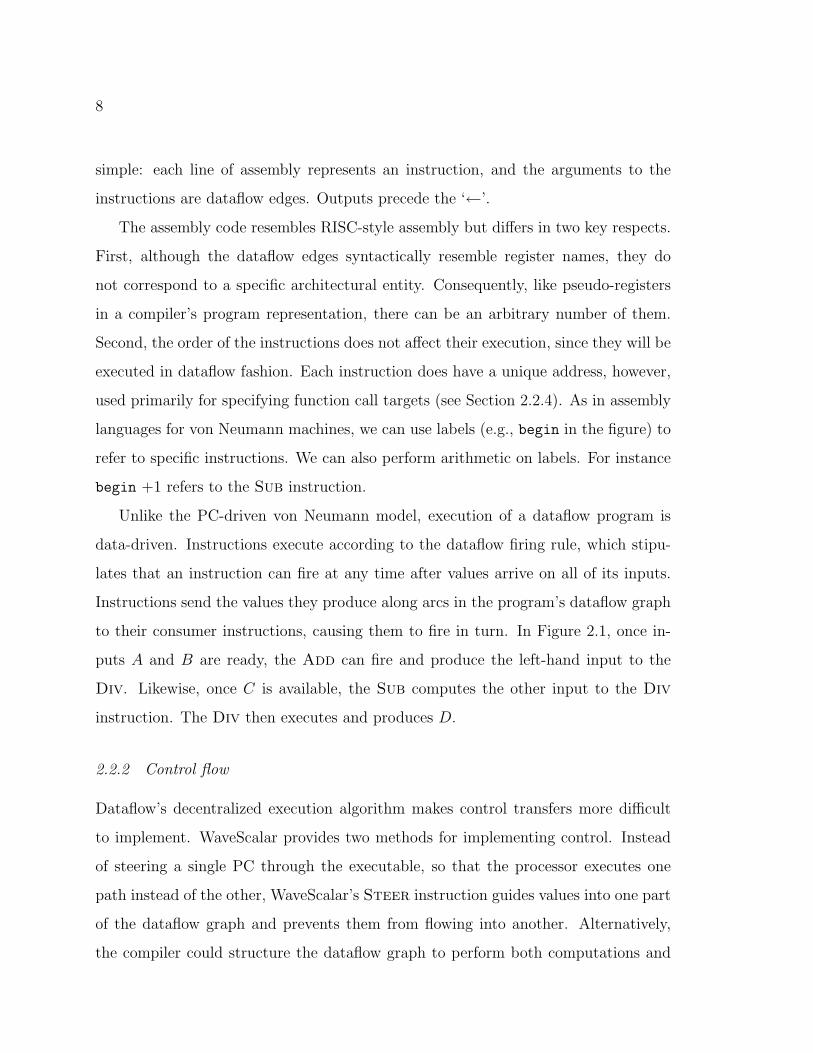
simple: each line of assembly represents an instruction, and the arguments to the
instructions are dataflow edges. Outputs precede the ‘ ’.
The assembly code resembles RISC-style assembly but di↵ers in two key respects.
First, although the dataflow edges syntactically resemble register names, they do
not correspond to a specific architectural entity. Consequently, like pseudo-registers
in a compiler’s program representation, there can be an arbitrary number of them.
Second, the order of the instructions does not a↵ect their execution, since they will be
executed in dataflow fashion. Each instruction does have a unique address, however,
used primarily for specifying function call targets (see Section 2.2.4). As in assembly
languages for von Neumann machines, we can use labels (e.g., begin in the figure) to
refer to specific instructions. We can also perform arithmetic on labels. For instance
begin +1 refers to the Sub instruction.
Unlike the PC-driven von Neumann model, execution of a dataflow program is
data-driven. Instructions execute according to the dataflow firing rule, which stipu-
lates that an instruction can fire at any time after values arrive on all of its inputs.
Instructions send the values they produce along arcs in the program’s dataflow graph
to their consumer instructions, causing them to fire in turn. In Figure 2.1, once in-
puts A and B are ready, the Add can fire and produce the left-hand input to the
Div. Likewise, once C is available, the Sub computes the other input to the Div
instruction. The Div then executes and produces D.
2.2.2 Control flow
Dataflow’s decentralized execution algorithm makes control transfers more di�cult
to implement. WaveScalar provides two methods for implementing control. Instead
of steering a single PC through the executable, so that the processor executes one
path instead of the other, WaveScalar’s Steer instruction guides values into one part
of the dataflow graph and prevents them from flowing into another. Alternatively,
the compiler could structure the dataflow graph to perform both computations and
9
if (A > 0)
D = C + B;
else
D = C - E;
F = D + 1; + -
S S
>0
S
+1
C B E
D D
A
F
+ ->0
C B EA
φ
+1
F
D
(A) (b) (c)
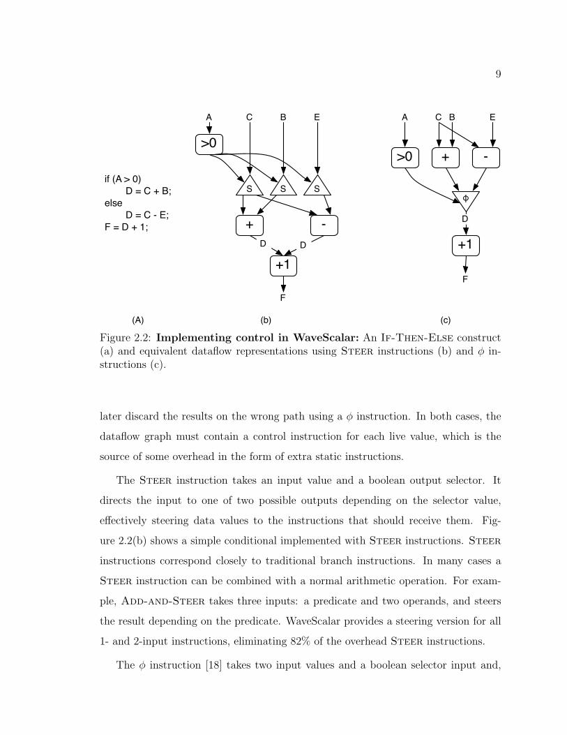
Figure 2.2: Implementing control in WaveScalar: An If-Then-Else construct(a) and equivalent dataflow representations using Steer instructions (b) and � in-structions (c).
later discard the results on the wrong path using a � instruction. In both cases, the
dataflow graph must contain a control instruction for each live value, which is the
source of some overhead in the form of extra static instructions.
The Steer instruction takes an input value and a boolean output selector. It
directs the input to one of two possible outputs depending on the selector value,
e↵ectively steering data values to the instructions that should receive them. Fig-
ure 2.2(b) shows a simple conditional implemented with Steer instructions. Steer
instructions correspond closely to traditional branch instructions. In many cases a
Steer instruction can be combined with a normal arithmetic operation. For exam-
ple, Add-and-Steer takes three inputs: a predicate and two operands, and steers
the result depending on the predicate. WaveScalar provides a steering version for all
1- and 2-input instructions, eliminating 82% of the overhead Steer instructions.
The � instruction [18] takes two input values and a boolean selector input and,

10
sum = 0;
for(i = 0; i < 5; i++)
sum += i;
const #0 const #0
+ +1
<5
S S
sum_first
sum_out
p
i_backedge
trigger
const #0 const #0
+ +1
<5
S S
WAWA
WA
(a) (b) (c)
waves
Figure 2.3: Loops in WaveScalar: Code for a simple loop (a), a slightly brokenimplementation (b), and the correct WaveScalar implementation (c).
depending on the selector, passes one of the inputs to its output. � instructions are
analogous to conditional moves and provide a form of predication. They remove the
selector input from the critical path of some computations and therefore increase par-
allelism, but they waste the e↵ort spent computing the unselected input. Figure 2.2(c)
shows � instructions in action.
2.2.3 Loops and waves
The Steer instruction may appear to be su�cient for WaveScalar to express loops,
since it provides a basic branching facility. However, in addition to branching,
dataflow machines must also distinguish dynamic instances of values from di↵erent
iterations of a loop. Figure 2.3(a) shows a simple loop that illustrates the problem
and WaveScalar’s solution.
Execution begins when data values arrive at the Const instructions, which inject
zeros into the body of the loop, one for sum and one for i (Figure 2.3(b)). On each
iteration through the loop, the left side updates sum and the right side increments i

11
and checks whether it is less than 5. For the first 5 iterations (i = 0 . . . 4), p is true
and the Steer instructions steer the new values for sum and i back into the loop.
On the last iteration, p is false, and the final value of sum leaves the loop via the
sum out edge. Since i is dead after the loop, the false output of the right-side Steer
instruction produces no output.
The problem arises because the dataflow execution model does not bound the
latency of communication over an arc and makes no guarantee that values arrive in
order. If sum first takes a long time to reach the Add instruction, the right side
portion of the dataflow graph could run ahead of the left side, generating multiple
values on i backedge and p. How would the Add and Steer instructions on the left
know which of these values to use? In this particular case, the compiler could solve
the problem by unrolling the loop completely, but this is not always possible.
Previous dataflow machines provided one of two solutions. In the first, static
dataflow [21, 20], only one value is allowed on each arc at any time. In a static
dataflow system, the dataflow graph as shown works fine. The processor would use
back-pressure to prevent the ’< 5’ and ’+1’ instructions from producing a new value
before the old values had been consumed. Static dataflow eliminates the ambiguity
between value instances, but it reduces parallelism because multiple iterations of a
loop cannot execute simultaneously. Similarly, multiple calls to a single function
cannot execute in parallel, making recursion impossible.
A second model, dynamic dataflow [56, 30, 35, 28, 50], tags each data value with
an identifier and allows multiple values to wait at the input to an instruction. The
combination of a data value and its tag is called a token. Dynamic dataflow machines
modify the dataflow firing rule so an instruction fires only when tokens with matching
tags are available on all its inputs. WaveScalar is a dynamic dataflow architecture.
Dynamic dataflow architectures di↵er in how they manage and assign tags to
values. In WaveScalar the tags are called wave-numbers [59]. We denote a WaveScalar
token with wave-number W and value v as <W>.v. WaveScalar assigns wave numbers
12
to compiler-defined, acyclic portions of the dataflow graph called waves. Waves are
similar to hyperblocks [41], but they are more general, since they can contain control-
flow joins and can have more than one entrance. Figure 2.3(c) shows the example
loop divided into waves (as shown by the dotted lines). At the top of each wave a set
of Wave-Advance instructions (the small diamonds) increments the wave numbers
of the values that passes through it.
Assume the code before the loop is wave number 0. When the code executes,
the two Const instructions each produce the token <0>.0 (wave number 0, value
0). The Wave-Advance instructions take these as input and output <1>.0, so the
first iteration executes in wave 1. At the end of the loop, the right-hand Steer
instruction will produce <1>.1 and pass it back to the Wave-Advance at the top
of its side of the loop, which will then produce <2>.1. A similar process takes place
on the left side of the graph. After 5 iterations the left Steer instruction produces
the final value of sum: <5>.10, which flows directly into the Wave-Advance at the
beginning of the follow-on wave.
With the Wave-Advance instructions in place, the right side can run ahead
safely, since instructions will only fire when the wave numbers in the operand tags
match. More generally, waves numbers allow instructions from di↵erent wave in-
stances, in this case iterations, to execute simultaneously.
Wave-numbers also play a key role in enforcing memory ordering (Chapter 3).
2.2.4 Function calls
Function calls on a von Neumann processor are fairly simple – the caller saves caller-
saved registers, pushes function arguments and the return address onto the stack (or
stores them in specific registers), and then uses a jump instruction to set the PC to
the address of the beginning of the called function, triggering its execution.
Dataflow architectures adopt a di↵erent convention. WaveScalar does not need to
preserve register values (there are no registers), but it must explicitly pass arguments
13
and a return address to the function and trigger its execution.
Passing arguments to a function creates a data dependence between the caller and
the callee. For indirect functions, these dependences are not statically known and
therefore the dataflow graph of the application does not contain them. To compen-
sate, WaveScalar provides an Indirect-Send instruction to send a data value to an
instruction at a computed address.
Indirect-Send takes as input the data value to send, a base address for the des-
tination instruction (usually a label), and the o↵set from that base (as an immediate).
For instance, if the base address is 0x1000, and the o↵set is 4, Indirect-Send sends
the data value to the instruction at 0x1004.
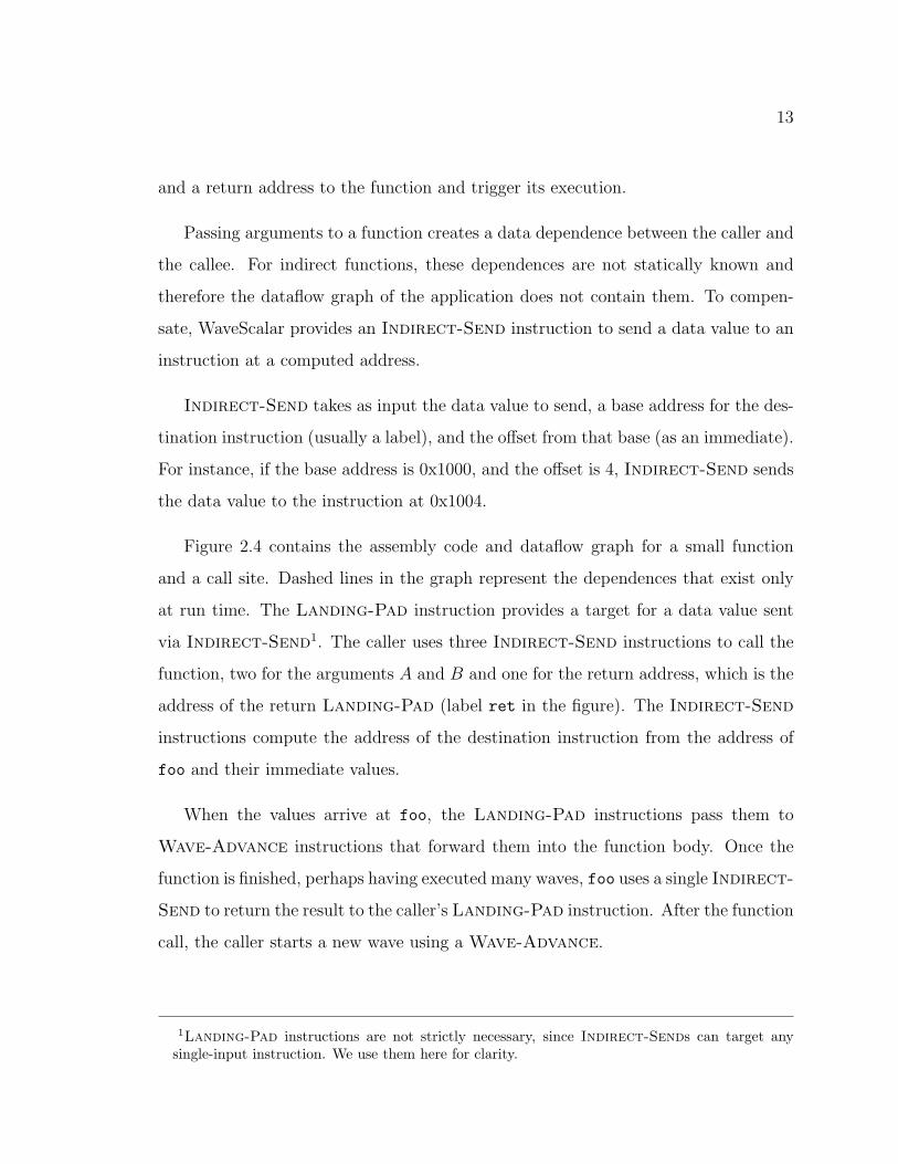
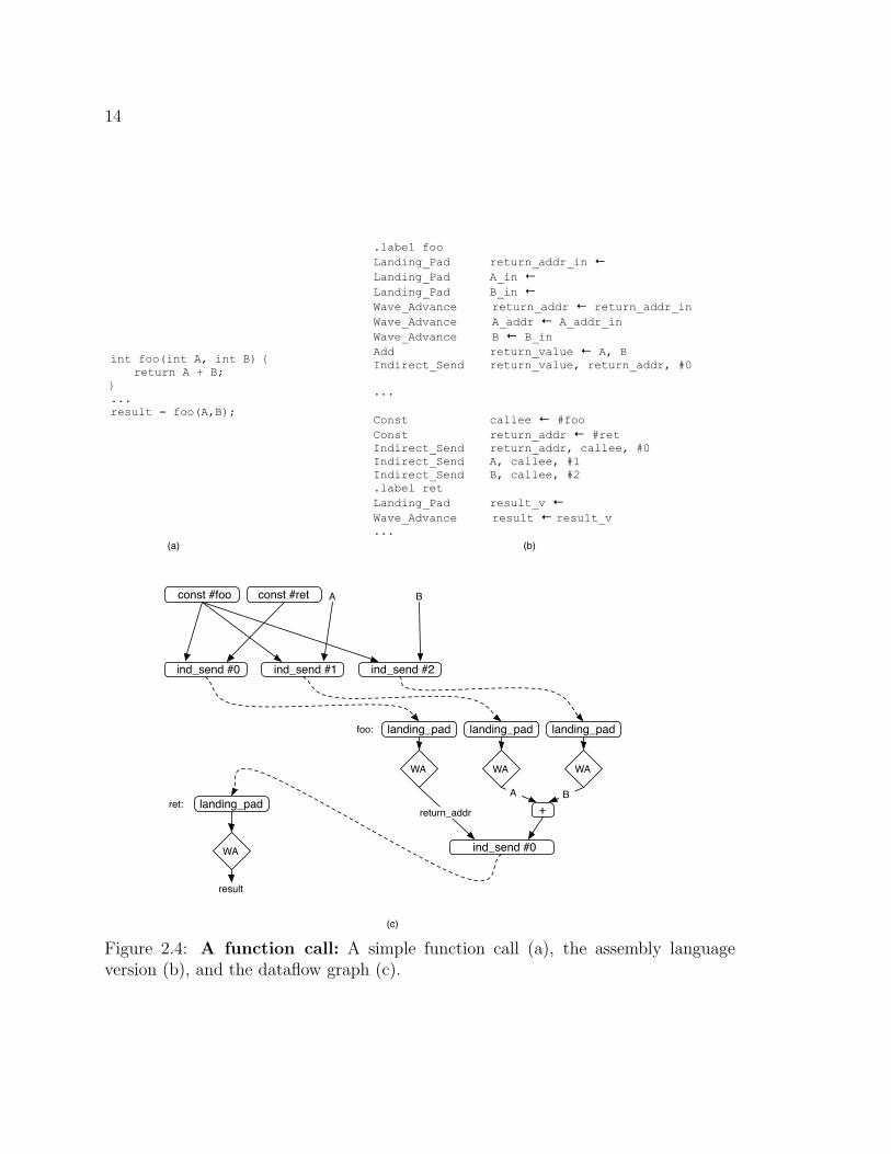
Figure 2.4 contains the assembly code and dataflow graph for a small function
and a call site. Dashed lines in the graph represent the dependences that exist only
at run time. The Landing-Pad instruction provides a target for a data value sent
via Indirect-Send1. The caller uses three Indirect-Send instructions to call the
function, two for the arguments A and B and one for the return address, which is the
address of the return Landing-Pad (label ret in the figure). The Indirect-Send
instructions compute the address of the destination instruction from the address of
foo and their immediate values.
When the values arrive at foo, the Landing-Pad instructions pass them to
Wave-Advance instructions that forward them into the function body. Once the
function is finished, perhaps having executed many waves, foo uses a single Indirect-
Send to return the result to the caller’s Landing-Pad instruction. After the function
call, the caller starts a new wave using a Wave-Advance.
1Landing-Pad instructions are not strictly necessary, since Indirect-Sends can target anysingle-input instruction. We use them here for clarity.
14
.label foo
Landing_Pad return_addr_in ←
Landing_Pad A_in ←
Landing_Pad B_in ←
Wave_Advance return_addr ← return_addr_in
Wave_Advance A_addr ← A_addr_in
Wave_Advance B ← B_in
Add return_value ← A, BIndirect_Send return_value, return_addr, #0
...
Const callee ← #foo
Const return_addr ← #retIndirect_Send return_addr, callee, #0Indirect_Send A, callee, #1Indirect_Send B, callee, #2.label ret
Landing_Pad result_v ←
Wave_Advance result ← result_v...
int foo(int A, int B) {return A + B;
}...result = foo(A,B);
(a) (b)
const #foo const #ret
ind_send #0 ind_send #1 ind_send #2
landing_pad
landing_pad
+
ind_send #0
A B
landing_pad landing_pad
return_addr
A B
foo:
WA WAWA
result
WA
ret:
(c)
Figure 2.4: A function call: A simple function call (a), the assembly languageversion (b), and the dataflow graph (c).

15
2.3 Discussion
The parts of the WaveScalar’s instruction set and execution model described in this
chapter borrow extensively from previous dataflow systems, but they do not include
facilities for accessing memory. The interface to memory is among the most impor-
tant components of any architecture, because changing memory is, from the outside
world’s perspective, the only thing a processor does. The next chapter describes the
fundamental incompatibility between pure dataflow execution and the linear ordering
of memory operations that von Neumann processors provide and imperative languages
rely upon. It also describe the interface WaveScalar provides to bridge this gap and
to allow von Neumann-style programs to run e�ciently on a dataflow machine.
16
Chapter 3
WAVE-ORDERED MEMORY
One of the largest obstacles to the success of previous dataflow architectures was
their inability to e�ciently execute programs written in conventional, imperative pro-
gramming languages. Imperative languages require memory operations to occur in a
strictly defined order to enforce data dependences through memory. Since these data
dependences are implicit (i.e., they do not appear in the program’s dataflow graph)
the dataflow execution model does not enforce them. WaveScalar surmounts this ob-
stacle by augmenting the dataflow model with a memory interface called wave-ordered
memory.
Wave-ordered memory capitalizes on wave and wave-number constructs defined
in Section 2.2.3. The compiler annotates memory operations within a wave with
ordering information so the memory system can “chain” the operations together in the
correct order. At runtime, the wave numbers provide ordering between the “chains”
of operations in each wave and, therefore, across all the operations in a program.
The next section defines the ordering problem. Section 3.2 describes the wave-
ordering scheme in detail. The section defines the wave-ordered memory annotations
and defines an abstract memory system that provides precise semantics for wave-
ordered memory. Section 3.3 describes an extension to the wave-ordered memory
scheme to express parallelism between operations.
We evaluate wave-ordered memory in Section 3.4 and compare it to another pro-
posed solution to the memory ordering problem, token-passing [12, 13]. We find that
wave-ordered memory reveals twice as much memory parallelism as token-passing and
investigate the reasons for the disparity.
17
Finally, Section 3.5 builds on the basics of wave-ordered memory to propose ex-
tensions to the system that may make it more e�cient in some scenarios. It also
presents sophisticated applications of wave-ordered memory aimed at maximizing
memory parallelism and exploiting alias information.
The focus of this chapter is on wave-ordered memory’s ability to express ordering
and memory parallelism independent of the architecture that incorporates it. We do
not address the hardware costs and trade-o↵s involved in implementing wave-ordered
memory, because those issues necessarily involve the entire architecture. Chapter 5
provides a thorough discussion of these issues in the WaveScalar processor architecture
and demonstrates that wave-ordered memory is practical in hardware.
3.1 Dataflow and memory ordering
This section describes the problem of enforcing imperative language memory ordering
in a dataflow environment. First, we define the ordering that imperative languages
require and discuss how von Neumann machines provide it. Then we demonstrate
why dataflow has trouble enforcing memory ordering.
3.1.1 Ordering in imperative languages
Imperative languages such as C and C++ provide a simple but powerful memory
model. Memory is a large array of bytes that programs access, reading and writing
bytes at will. To ensure correct execution, memory operations must (appear to) be
applied to memory in the order the programmer specifies (i.e., in program order).
In a traditional von Neumann processor, the program counter provides the req-
uisite sequencing information. It encounters memory operations as it steps through
the program and feeds them into the processor’s execution core. Modern processors
often allow instructions to execute out-of-order, but they must guarantee that the
instructions, especially memory instructions, execute in the order specified by the
PC.

18
Load
A[i+k] = x;
y = A[i];
+
Store
+
+
A ikx
y
j
Figure 3.1: Program order: A simple code fragment and the corresponding dataflowgraph demonstrating the dataflow memory ordering problem.
3.1.2 Dataflow execution
Dataflow ISAs only enforce the static data dependences in a program’s dataflow graph,
because they have no mechanism to ensure that memory operations occur in program
order. Figure 3.1 shows a dataflow graph that demonstrates this problem. The Load
must execute after the Store to ensure correct execution (dashed line), but conven-
tional dataflow instruction sets have di�culty expressing this ordering relationship,
because the relationship depend on runtime information (i.e., whether k is equal to
zero).
WaveScalar is the first dataflow instruction set and execution model that can
enforce the ordering between memory operations without unduely restricting the par-
allelism available in the dataflow graph. The next section describes wave-ordered
memory and how it enforces the implicit dependences that imperative languages de-
pend upon. Then we compare the scheme to an alternative solution and discuss
potential enhancements.

19
3.2 Wave-ordered memory
Wave-ordered memory provides the sequential memory semantics that imperative
programming languages require. Compiler-supplied annotations order the operations
within each wave (Section 2.2.3) of the program. The wave numbers associated with
each dynamic wave, which increase from one wave to the next, provide ordering
between waves. The combination of these two orderings provides a total order on all
the memory operations in the program.
Once we have described how wave-ordered memory fits into the WaveScalar model
from Chapter 2, we describe the annotations the compiler provides and how they
define the necessary ordering. Finally, we briefly discuss an alternative solution to
the dataflow memory ordering problem.
3.2.1 Adding memory to WaveScalar
Load and Store operations in WaveScalar programs fire according to the dataflow
firing rule, just as normal instructions do. When they execute they send a request
to the memory system that includes the current wave number and the annotations
described below. In response to Load operations, the memory system returns the
value read from memory. Store operations do not generate a response. WaveScalar
does not bound the delay between instruction execution and the request arriving
at the memory system or guarantee that operations will arrive in order. Previous
dataflow research refers to this type of memory interface as “split-phase” [16].
The split-phase interface provides two useful properties. First, it places few con-
straints on the memory system’s implementation. Second, it allows us to describe the
memory system without reference to the rest of the execution model. The description
of wave-ordered memory below exploits this fact extensively. For the purposes of
this chapter, all we need to know about WaveScalar execution is that it maintains
wave numbers properly and that memory requests eventually arrive at the memory
20
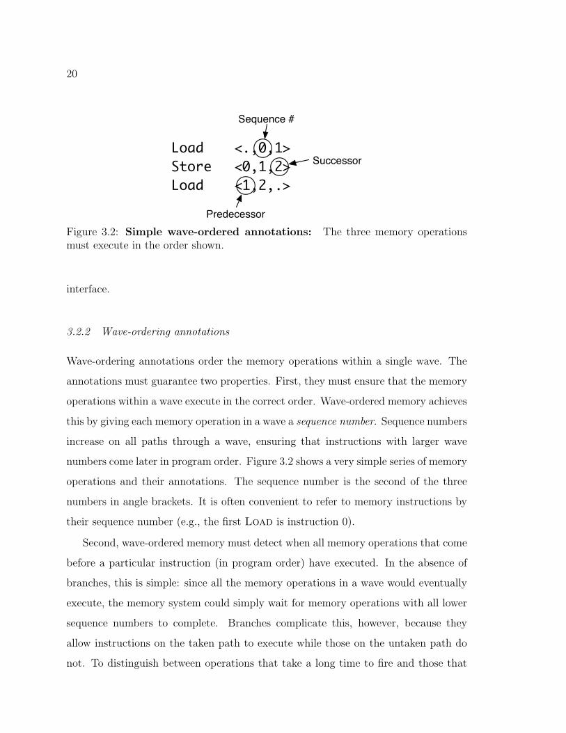
Load <.,0,1>
Store <0,1,2>
Load <1,2,.>
Sequence #
Predecessor
Successor
Figure 3.2: Simple wave-ordered annotations: The three memory operationsmust execute in the order shown.
interface.
3.2.2 Wave-ordering annotations
Wave-ordering annotations order the memory operations within a single wave. The
annotations must guarantee two properties. First, they must ensure that the memory
operations within a wave execute in the correct order. Wave-ordered memory achieves
this by giving each memory operation in a wave a sequence number. Sequence numbers
increase on all paths through a wave, ensuring that instructions with larger wave
numbers come later in program order. Figure 3.2 shows a very simple series of memory
operations and their annotations. The sequence number is the second of the three
numbers in angle brackets. It is often convenient to refer to memory instructions by
their sequence number (e.g., the first Load is instruction 0).
Second, wave-ordered memory must detect when all memory operations that come
before a particular instruction (in program order) have executed. In the absence of
branches, this is simple: since all the memory operations in a wave would eventually
execute, the memory system could simply wait for memory operations with all lower
sequence numbers to complete. Branches complicate this, however, because they
allow instructions on the taken path to execute while those on the untaken path do
not. To distinguish between operations that take a long time to fire and those that

21
Load <.,0,?>
Store <0,1,3> Store <0,2,3>
Load <?,3,.>
Load <.,0,?>
Store <0,2,3>
Load <?,3,.>
Matches forminga chain
Figure 3.3: Wave-ordering and control: Dashed boxes and lines denote basicblocks and control paths.
never will, each memory operation also carries the sequence number of the next and
previous operations in program order.
Figure 3.2 includes these annotations as well. The predecessor number is the first
number between the brackets, and the successor number is the last. The Store has
annotations <0, 1, 2>, because the Load with sequence number 0 precedes it and
the Load with sequence number 2 follows it. The ’.’ symbols indicate that there is
no predecessor of operation 0 and no successor of operation 2 in this wave.
At branch (join) points the successor (predecessor) number is unknown at compile
time, because control may take either path. In these cases a wildcard symbol, ‘?,’
takes the place of the successor (predecessor) number.
The left-hand portion of Figure 3.3 shows a simple if-then-else control flow
graph with wildcard annotations on operations 0 and 3. The right-hand portion
depicts how memory operations on the taken path are sequenced, described below.
Intuitively, the annotations allow the memory system to “chain” memory opera-
tions together. When the compiler generates and annotates a wave, there are many
potential chains of operations through the wave, but only one chain (i.e., one control
22
Load <.,0,?>
Store <0,1,2>
Load <?,2,.>
Load <.,0,?>
Store <0,1,3>
Load <?,3,.>
MemNop <0,2,3>
(a) (b)
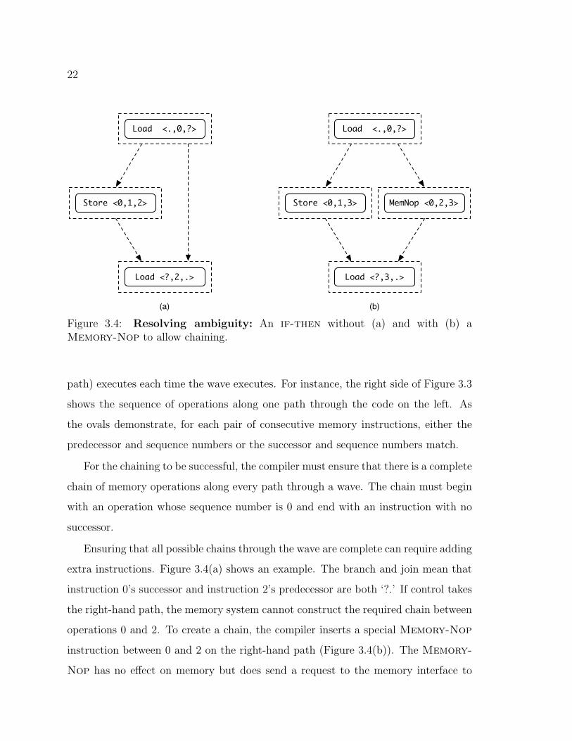
Figure 3.4: Resolving ambiguity: An if-then without (a) and with (b) aMemory-Nop to allow chaining.
path) executes each time the wave executes. For instance, the right side of Figure 3.3
shows the sequence of operations along one path through the code on the left. As
the ovals demonstrate, for each pair of consecutive memory instructions, either the
predecessor and sequence numbers or the successor and sequence numbers match.
For the chaining to be successful, the compiler must ensure that there is a complete
chain of memory operations along every path through a wave. The chain must begin
with an operation whose sequence number is 0 and end with an instruction with no
successor.
Ensuring that all possible chains through the wave are complete can require adding
extra instructions. Figure 3.4(a) shows an example. The branch and join mean that
instruction 0’s successor and instruction 2’s predecessor are both ‘?.’ If control takes
the right-hand path, the memory system cannot construct the required chain between
operations 0 and 2. To create a chain, the compiler inserts a special Memory-Nop
instruction between 0 and 2 on the right-hand path (Figure 3.4(b)). The Memory-
Nop has no e↵ect on memory but does send a request to the memory interface to
23
provide the missing link in the chain. Adding Memory-Nops introduces a small
amount of overhead, usually less than 3% of static instructions.
Once the compiler annotates the operations within each wave, the wave-ordered
memory system uses the information to enforce correct program behavior.
3.2.3 Formal ordering rules
To provide precise semantics for wave-ordered memory, we define an abstract memory
system that defines the range of correct behavior for a program that uses wave-ordered
memory. If a real memory system executes (or appears to execute) memory operations
in the same order as this abstract memory system, the real memory system is, by
definition, correct.
Describing an abstract memory system avoids the complications of an imple-
mentable design and does not tie the interface to a particular implementation. For
example, WaveScalar’s wave-ordering hardware restricts the number of sequence num-
bers in a wave, but other designs might not require such a constraint.
For each wave number, the abstract model maintains a list of memory requests,
called an operation bu↵er. The contents of operation bu↵ers are sorted by sequence
number. During execution, requests arrive from memory instructions that have fired
according to the dataflow firing rule. Memory requests may arrive in any order. When
operations are ready to be applied to memory, they issue to the memory system and
leave the operation bu↵er.
The current operation bu↵er is the first bu↵er (i.e., the bu↵er with the lowest
wave number) that contains un-issued operations. The algorithm below guarantees
that there is only one current bu↵er.
The predecessor, sequence, and successor numbers of a memory operation, M , are
pred(M), seq(M), and succ(M), respectively. The wavefront, F , is the most recently
issued operation in the current bu↵er.
When a request arrives, the wave-ordering mechanism routes it to the operation
24
bu↵er for the operation’s wave, inserts it into the bu↵er, and checks if it can issue
immediately.
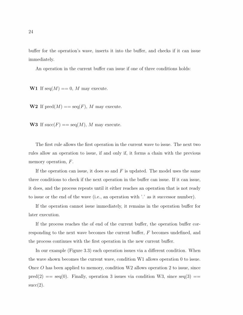
An operation in the current bu↵er can issue if one of three conditions holds:
W1 If seq(M) == 0, M may execute.
W2 If pred(M) == seq(F ), M may execute.
W3 If succ(F ) == seq(M), M may execute.
The first rule allows the first operation in the current wave to issue. The next two
rules allow an operation to issue, if and only if, it forms a chain with the previous
memory operation, F .
If the operation can issue, it does so and F is updated. The model uses the same
three conditions to check if the next operation in the bu↵er can issue. If it can issue,
it does, and the process repeats until it either reaches an operation that is not ready
to issue or the end of the wave (i.e., an operation with ’.’ as it successor number).
If the operation cannot issue immediately, it remains in the operation bu↵er for
later execution.
If the process reaches the of end of the current bu↵er, the operation bu↵er cor-
responding to the next wave becomes the current bu↵er, F becomes undefined, and
the process continues with the first operation in the new current bu↵er.
In our example (Figure 3.3) each operation issues via a di↵erent condition. When
the wave shown becomes the current wave, condition W1 allows operation 0 to issue.
Once O has been applied to memory, condition W2 allows operation 2 to issue, since
pred(2) == seq(0). Finally, operation 3 issues via condition W3, since seq(3) ==
succ(2).
25
3.2.4 Discussion
In addition to providing the semantics that imperative programming languages re-
quire, wave-ordered memory also provides the WaveScalar instruction set facility for
describing the control flow graph of an application. The predecessor, successor, and se-
quence numbers e↵ectively summarize the control flow graph for the memory system.
To our knowledge, WaveScalar is the first instruction set to explicitly provide high-
level structural information about the program. Wave-ordered memory demonstrates
that hardware can exploit this type of high-level information. Providing additional
information and developing architectures that can exploit it is an alluring avenue for
future research.
Next, we extend wave-ordered memory so the compiler can express additional
information about parallelism among memory operations.
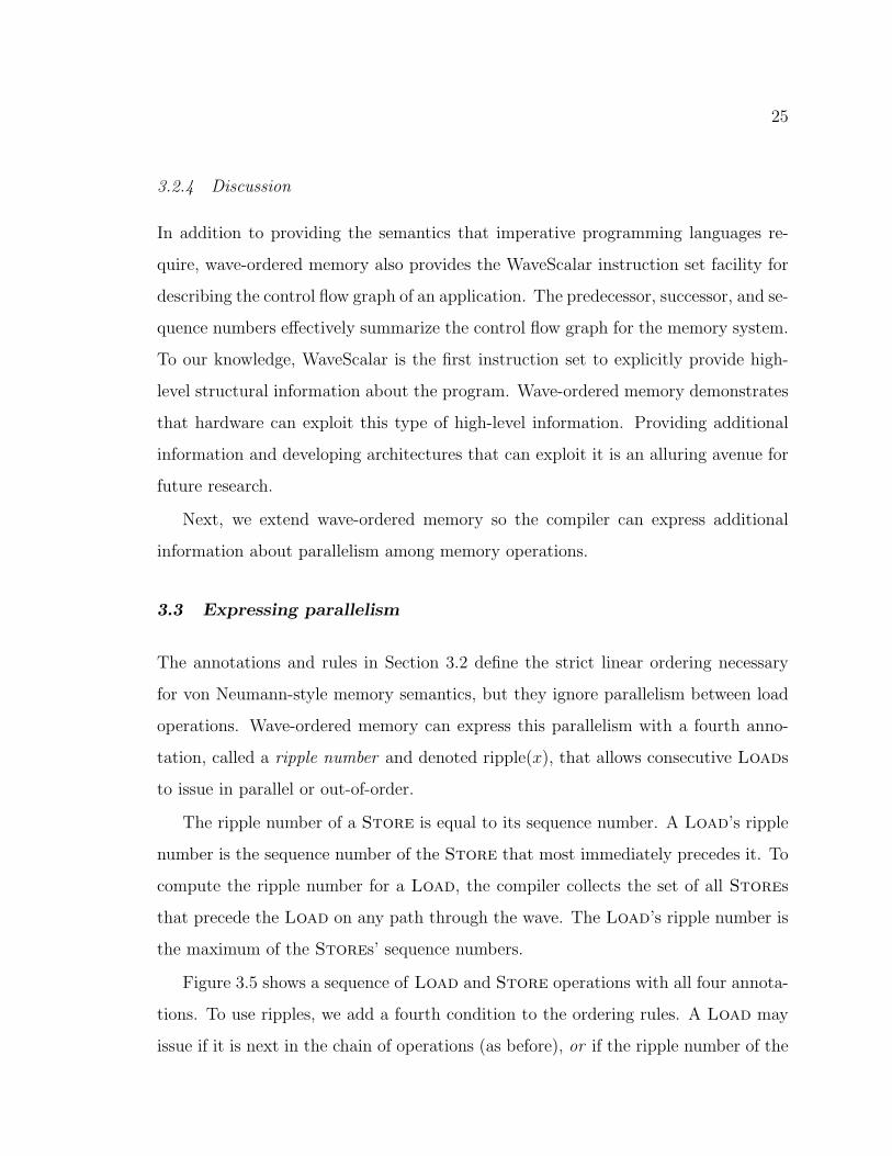
3.3 Expressing parallelism
The annotations and rules in Section 3.2 define the strict linear ordering necessary
for von Neumann-style memory semantics, but they ignore parallelism between load
operations. Wave-ordered memory can express this parallelism with a fourth anno-
tation, called a ripple number and denoted ripple(x), that allows consecutive Loads
to issue in parallel or out-of-order.
The ripple number of a Store is equal to its sequence number. A Load’s ripple
number is the sequence number of the Store that most immediately precedes it. To
compute the ripple number for a Load, the compiler collects the set of all Stores
that precede the Load on any path through the wave. The Load’s ripple number is
the maximum of the Stores’ sequence numbers.
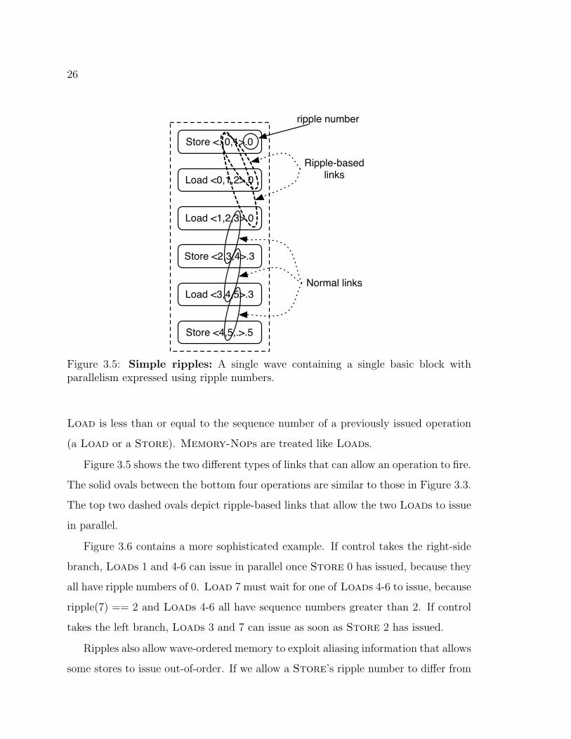
Figure 3.5 shows a sequence of Load and Store operations with all four annota-
tions. To use ripples, we add a fourth condition to the ordering rules. A Load may
issue if it is next in the chain of operations (as before), or if the ripple number of the
26
Store <.,0,1>.0
Load <0,1,2>.0
Load <1,2,3>.0
Store <2,3,4>.3
Store <4,5,.>.5
Load <3,4,5>.3Normal links
Ripple-basedlinks
ripple number
Figure 3.5: Simple ripples: A single wave containing a single basic block withparallelism expressed using ripple numbers.
Load is less than or equal to the sequence number of a previously issued operation
(a Load or a Store). Memory-Nops are treated like Loads.
Figure 3.5 shows the two di↵erent types of links that can allow an operation to fire.
The solid ovals between the bottom four operations are similar to those in Figure 3.3.
The top two dashed ovals depict ripple-based links that allow the two Loads to issue
in parallel.
Figure 3.6 contains a more sophisticated example. If control takes the right-side
branch, Loads 1 and 4-6 can issue in parallel once Store 0 has issued, because they
all have ripple numbers of 0. Load 7 must wait for one of Loads 4-6 to issue, because
ripple(7) == 2 and Loads 4-6 all have sequence numbers greater than 2. If control
takes the left branch, Loads 3 and 7 can issue as soon as Store 2 has issued.
Ripples also allow wave-ordered memory to exploit aliasing information that allows
some stores to issue out-of-order. If we allow a Store’s ripple number to di↵er from

27
Load <0,1,?>.0
Store <1,2,3>.2
Load <?,7,.>.2
Load <1,4,5>.0
Load <2,3,7>.2 Load <4,5,6>.0
Store <.,0,1>.0
Load <5,6,7>.0
Figure 3.6: Ripples and control: A more sophisticated application of ripple num-bers.
its sequence number, the wave-ordered interface can issue it according the same rules
that apply to Load operations. By applying ripples to easily-analyzed Stores (e.g.,
the stack or di↵erent fields in the same structure), the compiler can allow them to
issue in parallel.
3.4 Evaluation
Wave-ordered memory’s goal is to provide sequential memory semantics without in-
terfering with the parallelism that dataflow exposes. Therefore, the more parallelism
wave-ordered memory exposes, the better job it is doing. This section evaluates
wave-ordered memory and compares it to another ordering scheme called token pass-
ing [12, 13] by measuring the amount of memory parallelism each approach reveals.
It also describes an optimization that boosts wave-ordered memory’s e↵ectiveness by
taking advantage of runtime information.

28
3.4.1 Other approaches to dataflow memory ordering
Wave-ordered memory is not the only way to sequentialize memory operations in a
dataflow model. Researchers have proposed an alternative scheme that makes im-
plicit memory dependences explicit by adding a dataflow edge between each memory
operation and the next [12, 13]. While this token passing scheme is simple, our results
show that wave-ordered memory expresses twice as much memory parallelism.
Despite this, token-passing is very useful in some situations, because it gives the
programmer or compiler complete control over memory ordering. If very good memory
aliasing information is available, the programmer or compiler can express parallelism
directly by judiciously placing dependences only between those memory operations
that must actually execute sequentially. WaveScalar provides a simple token-passing
facility for just this purpose (Chapter 8).
3.4.2 Methodology
Our focus is on the expressive power of wave-ordered memory, not a particular proces-
sor architecture, so we use an idealized dataflow processor based on WaveScalar’s ISA
to evaluate wave-ordered memory. The processor has infinite execution resources and
memory bandwidth. Memory requests travel from the instructions to the memory
interface in a single cycle. Likewise data messages from one dataflow instruction to
another require a single cycle.
To generate dataflow executables, we compile applications with the DEC cc com-
piler using -O4 optimizations. A binary translator-based tool-chain converts these
binaries into dataflow executables. The binary translator does not perform any alias
analysis and uses a simple wave-creation algorithm. The wave-ordering mechanism
is a straightforward implementation of the algorithm outlined in Section 3.2. All
execution is non-speculative.
To compare wave-ordered memory to token-passing, we modify the binary trans-

29
0
0.2
0.4
0.6
0.8
1
1.2
1.4
ammp
art
equa
kegz
ipmcf
twolf
Mem
ory I
nstr
ucti
on
s/
Cycle
token-passing
wave-ordered, no
ripples
wave-ordered
wave-ordered + store
decoupling
Figure 3.7: Memory parallelism: A comparison of Wave-ordered memory andtoken-passing.
lator to use a simple token-passing scheme similar to [13] instead of wave-ordered
memory.
We use a selection of the Spec2000 [58] benchmark suite: ammp, art, equake, gzip,
mcf and twolf. We do not use all of the spec suite due to limitations of our binary
translator. We run each workload for 500 million instructions.
3.4.3 Results
Figure 3.7 shows the number of memory instructions executed per cycle (MIPC)
for four di↵erent ordering schemes. The first bar in each group is token-passing.
The second bar is wave-ordered memory without ripple annotations (i.e., no load
parallelism) and the third bar full-blown wave-ordered memory. The next section
describes the last bar.
Comparing the first two bars reveals that wave-ordered memory exposes twice as
much MIPC as token-passing on average, corresponding to a 46% increase in overall
IPC. The di↵erence is primarily due to the steering dataflow machines use for con-
trol flow. The memory token is a normal data value, so the compiler must insert
Steer instructions to guide it along the path of execution. The Steer instructions

30
introduce additional latency that can delay the execution of memory operations. In
our applications, there are an average of 2.5 Steer instructions between each pair of
consecutive memory operations.
Wave-ordered memory avoids this overhead by encoding the necessary control
flow information in the wave-ordering annotations. When the requests arrive at the
memory interface they carry that information with them. The wavefront, F , from the
algorithm in Section 3.2 serves the same conceptual purpose as the token: It moves
from operation to operation, allowing them to fire in the correct order, but it does
not traverse any non-memory instructions.
The graph also shows that between 0 and 5% of wave-ordered memory’s memory
parallelism comes from its ability to express load parallelism. If that is all the rip-
ple annotations can achieve, their value is dubious. However, our binary translator
performs no alias analysis and the waves it generates often contain few memory oper-
ations. We believe that a more sophisticated compiler will use ripples more e↵ectively.
Section 3.5 describes two promising approaches for generating larger waves that we
will investigate in the future.
3.4.4 Decoupling store addresses and data
Wave-ordered memory can incorporate simple run-time memory disambiguation by
taking advantage of the fact that the address for a Store is sometimes ready before
the data value. If the memory system knew the address as soon as it was available,
it could safely proceed with future memory operations to di↵erent addresses.
To incorporate this approach into wave-ordered memory, we break Store opera-
tions into two instructions, one to send the address and the other to forward the data
to the memory interface.
If the store address arrives first, it is called a partial store. The wave-ordering
mechanism treats it as a normal store operation (i.e., it issues according the rules in
Section 3.2, as usual). When a partial Store issues, the memory system assigns it a

31
partial store queue to hold future operations to the same address. Whenever an oper-
ation issues, the memory system checks its address against all the outstanding partial
stores. If it matches one of their addresses, it goes to the end of the corresponding
partial store queue. When the data for the store finally arrives, the memory system
can apply all the operations in the partial store queue in quick succession.
If the data for a store arrives first, the memory system does nothing, and waits
for the address to arrive. When the address arrives, the memory interface handles
the store as in the normal case.
The fourth bar in Figure 3.7 shows the performance of wave-ordered memory with
decoupled stores. To ensure a fair comparison, the instructions that send the store
data to memory are not counted. Decoupling address and data increases memory
parallelism by 30% on average and between 21% and 46% for individual applications.
3.5 Future directions
Wave-ordered memory solves the memory ordering problem for dataflow machines and
outperforms token passing, but there is still room for improvement. In particular, the
binary-translator constrains our current implementation of wave-ordered memory and
makes implementing aggressive optimizations di�cult. We are currently building a
custom dataflow compiler that will be free of these constraints. This section describes
several of our ideas for compiler-based improvements to wave-ordered memory. In
addition, it outlines a second approach to incorporating alias analysis into wave-
ordered memory.
3.5.1 Sequence number reuse
Section 3.2.2 suggests assigning each operation in a wave a unique sequence number.
Since sequence numbers must be expressed in a fixed number of bits, they are a finite
resource and might be scarce. The compiler can reuse sequence numbers so long as
it guarantees that the sequence numbers always increase along any path and no two
32
Load <0,1,2>.0
Store <1,2,4>.2
Load <4,5,.>.2
Load <1,2,3>.0
Load <2,4,5>.2 Load <2,3,4>.0
Store <.,0,1>.0
Load <3,4,5>.0
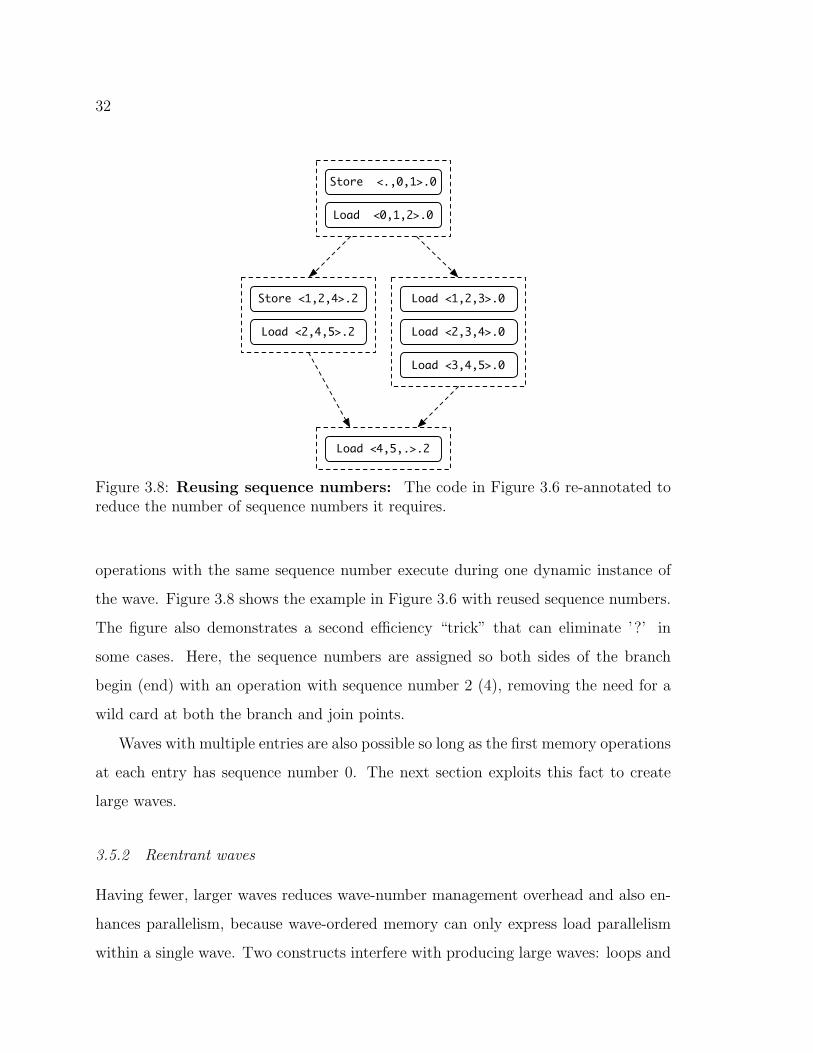
Figure 3.8: Reusing sequence numbers: The code in Figure 3.6 re-annotated toreduce the number of sequence numbers it requires.
operations with the same sequence number execute during one dynamic instance of
the wave. Figure 3.8 shows the example in Figure 3.6 with reused sequence numbers.
The figure also demonstrates a second e�ciency “trick” that can eliminate ’?’ in
some cases. Here, the sequence numbers are assigned so both sides of the branch
begin (end) with an operation with sequence number 2 (4), removing the need for a
wild card at both the branch and join points.
Waves with multiple entries are also possible so long as the first memory operations
at each entry has sequence number 0. The next section exploits this fact to create
large waves.
3.5.2 Reentrant waves
Having fewer, larger waves reduces wave-number management overhead and also en-
hances parallelism, because wave-ordered memory can only express load parallelism
within a single wave. Two constructs interfere with producing large waves: loops and

33
Slow-path;no loop or func. calls
Fast-path
Slow-pathw/ loop
Fast-path
(a) (b)
Waves
Figure 3.9: Loops break up waves: A block of code in a single wave (a) and brokenup by a loop (b).
function calls.
Many functions contain a common case “fast-path” that executes frequently and
quickly in addition to slower paths that handle exceptional or unusual cases. If the
slow paths contain loops or function calls (e.g., to an error handling routine), the
function can end up broken into many, small waves.
Figure 3.9 shows why this occurs. Both sides of the figure show similar code.
The right-hand path is the fast-path and the left side contains infrequently executed,
slow-path code. In Figure 3.9(a) the slow-path code contains ordinary instructions,
so the entire code fragment is a single wave. In Figure 3.9(b) the slow-path code
includes a loop. Since waves cannot contain back edges, a naive compiler might break
the code into three waves, as shown. This incurs extra wave-management overhead
and eliminates load-parallelism between the two waves that now make up the fast
path.

34
Loop Body
Load <?,2,.>.0
Load <0,1,2>.0
Store <.,0,?>.0
Noop <.,0,2>.0
Wave
Wave
Figure 3.10: A reentrant wave: A wave with multiple entrances to preserve paral-lelism on the fast path.
Figure 3.10 demonstrates a more sophisticated solution. In the common case,
control follows the right-hand path and executes in a single wave. Alternatively,
control leaves the large wave, and enters the wave for the loop. When the loop is
complete, control enters the large wave again but by a second entrance. Setting
Memory-Nop instruction’s successor number to 2 informs the memory system that
operation 1 will not execute. Now, only the slow path incurs extra wave-management
overhead, and the parallelism between Loads 1 and 2 remains.
3.5.3 Alias analysis
Our binary translator does not have enough information to perform aggressive alias
analysis, so it is di�cult to evaluate how useful ripples are for expressing the infor-
mation alias analysis would provide. Other approaches to expressing parallelism may
prove more e↵ective.
One alternative approach would allow the chains of operations to “fork” and “join”

35
so that independent sequences of operations could run in parallel. Within each par-
allel chain, operations would be ordered as usual. For instance, in a strongly typed
language, the compiler could provide a separate chain for accessing objects of a par-
ticular type, because accesses to variables of di↵erent types are guaranteed not to
conflict.
3.6 Discussion
Adding wave-ordered memory to the WaveScalar ISA in Chapter 2 provides the last
piece necessary for WaveScalar to replace the von Neumann model in modern, single-
threaded computer systems. The resulting instruction set is more complex than a
conventional RISC ISA, but we have not found the complexity di�cult to handle in
our WaveScalar toolchain.
In return for the complexity, WaveScalar provides three significant benefits. First,
wave-ordered memory allows WaveScalar to e�ciently provide the semantics that im-
perative languages require and to express parallelism among Load operations. Sec-
ond, WaveScalar can express instruction-level parallelism explicitly, while still main-
taining these conventional memory semantics. Third, WaveScalar’s execution model
is distributed. Instructions only communicate if they must. There is no centralized
control point.
In the next section we describe a microarchitecture that implements the WaveScalar
ISA. We find that, in addition to increasing instruction-level parallelism, the WaveScalar
instruction set allows the microarchitecture to be substantially simpler than a modern,
out-of-order superscalar.

36
Chapter 4
A WAVESCALAR ARCHITECTURE FORSINGLE-THREADED PROGRAMS
WaveScalar’s overall goal is to enable an architecture that avoids the scaling
problems described in Chapter 1. This chapter describes a tile-based WaveScalar
architecture, called the WaveCache, that addresses those problems. The WaveCache
comprises everything, except main memory, required to run a WaveScalar program.
It contains a scalable grid of simple, identical dataflow processing elements, wave-
ordered memory hardware, and a hierarchical interconnect to support communication.
Each level of the hierarchy uses a separate communication structure: high-bandwidth,
low-latency systems for local communication, and slower, narrower communication
mechanisms for long distance communication.
As we will show, the WaveCache directly addresses two of the challenges we out-
lined in the introduction. First, the WaveCache contains no long wires. As the size
of the WaveCache increases, the lengths of the longest wires do not. Second, the
WaveCache architecture scales easily from small designs suitable for executing a sin-
gle thread to much larger designs suited to multi-threaded workloads (see Chapter 5).
The larger designs contain more tiles, but the tile structure, and therefore, the overall
design complexity do not change. The challenge of defect and fault tolerance is the
subject of ongoing research. The WaveCache’s decentralized, uniform structure sug-
gests that it would be easy to disable faulty components to tolerate manufacturing
defects.
We begin by summarizing the WaveCache’s design and operation at a high level
in Section 4.1. Next, Sections 4.2 to 4.7 provide a more detailed description of its

37
PE
Cluster
DomainPod
L2
L2
L2
L2
L2 L2
Net-
work
D$S
B
D$
D$
D$
Figure 4.1: The WaveCache: The hierarchical organization of the microarchitectureof the WaveCache.
major components and how they interact. The next chapter evaluates the design.
4.1 WaveCache architecture overview
Several recently proposed architectures, including the WaveCache, take a tile-based
approach to addressing future scaling problems [46, 53, 39, 42, 26, 13]. Instead of
designing a monolithic core that comprises the entire die, tiled processors cover the die
with many identical tiles, each of which is a complete, though simple, processing unit.
Since they are less complex than the monolithic core and are replicated across the die,
tiled architectures quickly amortize design and verification costs. Tiled architectures
generally compute under decentralized control, contributing to shorter wire lengths.
Finally, they can be designed to tolerate manufacturing defects in some portion of
the tiles.
In the WaveCache, each tile is called a cluster (Figure 4.1). A cluster contains four
identical domains, each with eight identical processing elements (PEs). In addition,
each cluster has an L1 data cache, wave-ordered memory interface hardware, and a
network switch for communicating with adjacent clusters.
38
#0
#0
+
+1
<5S
S
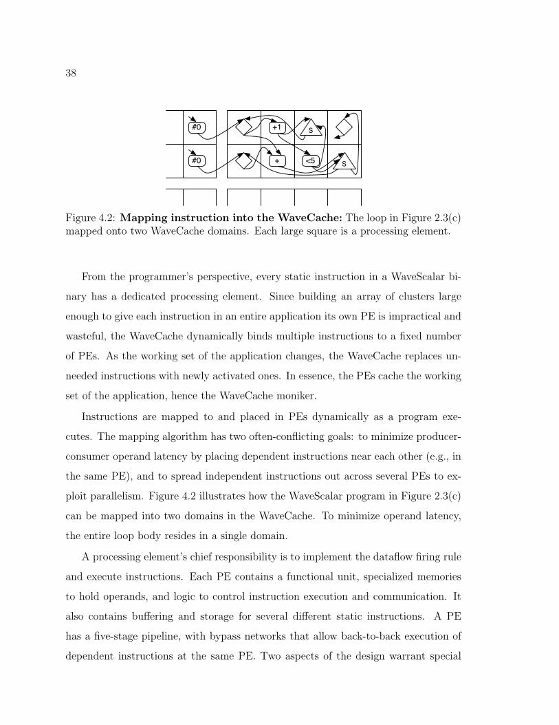
Figure 4.2: Mapping instruction into the WaveCache: The loop in Figure 2.3(c)mapped onto two WaveCache domains. Each large square is a processing element.
From the programmer’s perspective, every static instruction in a WaveScalar bi-
nary has a dedicated processing element. Since building an array of clusters large
enough to give each instruction in an entire application its own PE is impractical and
wasteful, the WaveCache dynamically binds multiple instructions to a fixed number
of PEs. As the working set of the application changes, the WaveCache replaces un-
needed instructions with newly activated ones. In essence, the PEs cache the working
set of the application, hence the WaveCache moniker.
Instructions are mapped to and placed in PEs dynamically as a program exe-
cutes. The mapping algorithm has two often-conflicting goals: to minimize producer-
consumer operand latency by placing dependent instructions near each other (e.g., in
the same PE), and to spread independent instructions out across several PEs to ex-
ploit parallelism. Figure 4.2 illustrates how the WaveScalar program in Figure 2.3(c)
can be mapped into two domains in the WaveCache. To minimize operand latency,
the entire loop body resides in a single domain.
A processing element’s chief responsibility is to implement the dataflow firing rule
and execute instructions. Each PE contains a functional unit, specialized memories
to hold operands, and logic to control instruction execution and communication. It
also contains bu↵ering and storage for several di↵erent static instructions. A PE
has a five-stage pipeline, with bypass networks that allow back-to-back execution of
dependent instructions at the same PE. Two aspects of the design warrant special
39
notice. First, it avoids a large, centralized tag matching store found on some previ-
ous dataflow machines. Second, although PEs dynamically schedule execution, the
scheduling hardware is dramatically simpler than a conventional dynamically sched-
uled processor. Section 4.2 describes the PE design in more detail.
To reduce communication costs between PEs in the processor, the architecture or-
ganizes PEs hierarchically along with their communication infrastructure (Figure 4.1).
They are first coupled into pods ; PEs within a pod snoop each others’ ALU bypass
networks and share instruction scheduling information, and therefore achieve the same
back-to-back execution of dependent instructions as a single PE. The pods are fur-
ther grouped into domains; within a domain, PEs communicate over a set of pipelined
broadcast buses. The four domains in a cluster communicate point-to-point over a
local switch. At the top level, clusters communicate over an on-chip interconnect
built from the network switches in the clusters.
PEs access memory by sending requests to the wave-ordered memory interface in
their cluster (see Section 4.4). The interface accepts the message if it is handling
requests for the wave the request belongs to. Otherwise, it forwards it to the wave-
ordered interface at the appropriate cluster. Section 4.4 describes the process for
mapping waves to wave-ordered interfaces.
Once a memory operation issues from the wave-ordered interface, the local L1
cache provides the data, if possible. Otherwise, it initiates a conventional cache
coherence request to retrieve the data from the L2 cache (located around the edge
of the array of clusters, along with the coherence directory) or the L1 cache that
currently owns the data.
A single cluster, combined with an L2 cache and traditional main memory, is
su�cient to run any WaveScalar program, albeit possibly with poor performance as
instructions are swapped in and out of the small number of available PEs. To build
larger and higher performing machines, multiple clusters are connected by an on-chip
network. A traditional directory-based MOESI protocol with multiple readers and a

40
single writer maintains cache coherence.
4.2 The processing element
At a high level, the structure of a PE pipeline resembles a conventional five-stage,
dynamically scheduled execution pipeline. The biggest di↵erence is that the PE’s
execution is entirely data-driven. Instead of executing instructions provided by a
program counter, as you find on von Neumann machines, values (i.e., tokens) arrive
at a PE destined for a particular instruction. The arrival of all of an instruction’s
input values triggers its execution – the essence of dataflow execution.
Our goal in designing the PE was to meet our cycle-time goal while still enabling
dependent instructions to execute on consecutive cycles. Pipelining was relatively
simple. Back-to-back execution, however, was the source of significant complexity.
In order, the PE’s pipeline stages are:
Input: Operand messages arrive at the PE either from another PE or from itself
(via the ALU bypass network). The PE may reject messages if too many arrive in
one cycle; the senders will then retry on a later cycle.
Match: After they leave Input, operands enter the matching table, where tag
matching occurs. Cost-e↵ective matching is essential to an e�cient dataflow design
and has historically been an impediment to more e↵ective dataflow execution. The
key challenge in designing the WaveCache matching table was emulating a potentially
infinite table with a much smaller physical structure. This problem arises, because
WaveScalar is a dynamic dataflow architecture, and places no limit on the number
of dynamic instances of a static instruction that may reside in the matching table,
waiting for input operands to arrive. To address this challenge, the matching table is
implemented as a specialized cache for a larger in-memory matching table – a common
dataflow technique [30, 56].

41
The matching table is associated with a tracker board, which determines when an
instruction has a complete set of inputs, and is therefore ready to execute. When this
occurs, the instruction moves into the scheduling queue.
Dispatch: The PE selects an instruction from the scheduling queue, reads its
operands from the matching table and forwards them to Execute. If the destination
of the dispatched instruction is local, it speculatively issues the consumer instruction
to the scheduling queue, enabling its execution on the next cycle.
Execute: In most cases Execute executes an instruction and sends its results to
Output, which broadcasts it over the bypass network. However, there are two cases
in which execution will not occur. First, if an instruction was dispatched speculatively
and one of its operands has not yet arrived, the instruction is squashed. Second, if
Output is full, Execute stalls until space becomes available.
Output: Instruction outputs are sent via the output bus to their consumer instruc-
tions, either at this PE or a remote PE. The output bu↵er broadcasts the value on the
PE’s broadcast bus. In the common case, a consumer PE within that domain accepts
the value immediately. It is possible, however, that the consumer cannot handle the
value that cycle and will reject it. The round-trip to send the value and receive an
Ack/Nack reply takes four cycles. Rather than have the data value occupy the
output register for that period, the PE assumes it will be accepted, moving it into its
4-entry reject bu↵er, and inserts a new value into the output bu↵er on the next cycle.
If an operand ends up being rejected, it is fed back into the output queue to be sent
again to the destinations that rejected it. When all the receivers have accepted the
value, the reject bu↵er discards it.
Figure 4.3 illustrates how instructions from a simple dataflow graph (on the left
side of the figure) flow through the WaveCache pipeline. It also illustrates how the
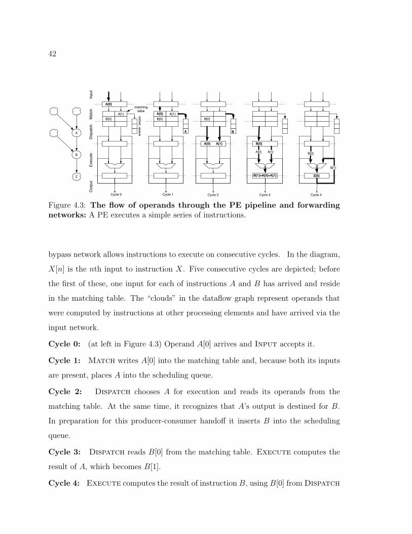
42
A
B
Z
A[0] A[1]
B[0]
B
B[0]
Z[0]
A[0] A[1]
B[1]
B[0]
B[1]=A[0]+A[1]
B[0]
sched. q
ueue
Inp
ut
Ma
tch
Dis
pa
tch
Exe
cu
teO
utp
ut
A[0]
A
A[1]
B[0]
matchingtable
A[0]
Cycle 0 Cycle 1 Cycle 2 Cycle 3 Cycle 4
A[1]
BA
Figure 4.3: The flow of operands through the PE pipeline and forwardingnetworks: A PE executes a simple series of instructions.
bypass network allows instructions to execute on consecutive cycles. In the diagram,
X[n] is the nth input to instruction X. Five consecutive cycles are depicted; before
the first of these, one input for each of instructions A and B has arrived and reside
in the matching table. The “clouds” in the dataflow graph represent operands that
were computed by instructions at other processing elements and have arrived via the
input network.
Cycle 0: (at left in Figure 4.3) Operand A[0] arrives and Input accepts it.
Cycle 1: Match writes A[0] into the matching table and, because both its inputs
are present, places A into the scheduling queue.
Cycle 2: Dispatch chooses A for execution and reads its operands from the
matching table. At the same time, it recognizes that A’s output is destined for B.
In preparation for this producer-consumer hando↵ it inserts B into the scheduling
queue.
Cycle 3: Dispatch reads B[0] from the matching table. Execute computes the
result of A, which becomes B[1].
Cycle 4: Execute computes the result of instruction B, using B[0] from Dispatch

43
PE PE
PE PE PE PE
PE PE
PE PE
PE PE PE PE
PE PE
PE PE
PE PE PE PE
PE PE
PE PE
PE PE PE PE
PE PE
StoreBufferD$
Switch
Netpseudo PE
Mempseudo PE
Netpseudo PE
Mempseudo PE
Net pseudo PE
Mempseudo PE
Net pseudo PE
Mempseudo PE
North
South
East
West
domain
pod intra-clusterinterconnect
inter-clusterswitch
intra-domaininterconnect
pod bypassing
Figure 4.4: The cluster interconnects: A high-level picture of a cluster illustratingthe interconnect organization.
and B[1] from the bypass network.
Cycle 5 (not shown): Output will send B’s result to instruction Z.
The logic in Match and Dispatch is the most complex part of the entire Wave-
Cache architecture, and most of it is devoted to allowing back-to-back execution of
dependent instructions while achieving our cycle time goal (22FO4).
4.3 The WaveCache interconnect
The previous section described the execution resource of the WaveCache, the PE. This
section will detail how PEs on the same chip communicate. PEs send and receive
data using a hierarchical, on-chip interconnect (Figure 4.4). The figure shows the
four levels in this hierarchy: intra-pod, intra-domain, intra-cluster and inter-cluster.
While the purpose of each network is the same – transmission of instruction operands
and memory values – their designs vary significantly. We will describe the salient
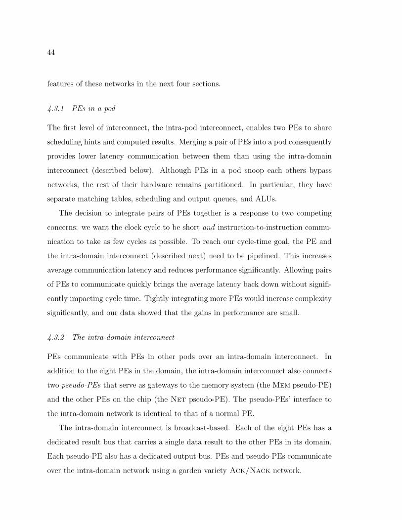
44
features of these networks in the next four sections.
4.3.1 PEs in a pod
The first level of interconnect, the intra-pod interconnect, enables two PEs to share
scheduling hints and computed results. Merging a pair of PEs into a pod consequently
provides lower latency communication between them than using the intra-domain
interconnect (described below). Although PEs in a pod snoop each others bypass
networks, the rest of their hardware remains partitioned. In particular, they have
separate matching tables, scheduling and output queues, and ALUs.
The decision to integrate pairs of PEs together is a response to two competing
concerns: we want the clock cycle to be short and instruction-to-instruction commu-
nication to take as few cycles as possible. To reach our cycle-time goal, the PE and
the intra-domain interconnect (described next) need to be pipelined. This increases
average communication latency and reduces performance significantly. Allowing pairs
of PEs to communicate quickly brings the average latency back down without signifi-
cantly impacting cycle time. Tightly integrating more PEs would increase complexity
significantly, and our data showed that the gains in performance are small.
4.3.2 The intra-domain interconnect
PEs communicate with PEs in other pods over an intra-domain interconnect. In
addition to the eight PEs in the domain, the intra-domain interconnect also connects
two pseudo-PEs that serve as gateways to the memory system (the Mem pseudo-PE)
and the other PEs on the chip (the Net pseudo-PE). The pseudo-PEs’ interface to
the intra-domain network is identical to that of a normal PE.
The intra-domain interconnect is broadcast-based. Each of the eight PEs has a
dedicated result bus that carries a single data result to the other PEs in its domain.
Each pseudo-PE also has a dedicated output bus. PEs and pseudo-PEs communicate
over the intra-domain network using a garden variety Ack/Nack network.

45
4.3.3 The intra-cluster interconnect
The intra-cluster interconnect provides communication between the four domains’
Net pseudo-PEs. It also uses a Ack/Nack network similar to that of the intra-
domain interconnect.
4.3.4 The inter-cluster interconnect
The inter-cluster interconnect is responsible for all long-distance communication in
the WaveCache. This includes operands traveling between PEs in distant clusters
and coherence tra�c for the L1 caches.
Each cluster contains an inter-cluster network switch, that routes messages be-
tween six input/output ports: four of the ports lead to the network switches in the
four cardinal directions, one is shared among the four domains’ Net pseudo-PEs, and
one is dedicated to the store bu↵er and L1 data cache.
Each input/output port supports the transmission of up to two operands. Its
routing follows a simple protocol: the current bu↵er storage state (i.e., whether space
is available or not) for each cardinal direction at each switch is sent to the adjacent
switch in that direction. The adjacent switches receive this information a clock cycle
later, and will only send data if the receiver is guaranteed to have space.
The inter-cluster switch provides two virtual channels that the interconnect uses
to prevent deadlock [19]. Each output port contains two 8-entry output queues (one
for each virtual network). In some cases, a message may have two possible directions
(e.g., North and West if its ultimate destination is to the northwest). In these cases
the router randomly selects which way to route the message.
4.4 The store bu↵er
The hardware support for wave-ordered memory lies in the WaveCache’s store bu↵ers.
The store bu↵ers, one per cluster, are responsible for implementing the wave-ordered

46
Readycheck
route to partial store?
Data Cache
Input arbitration
partial storequeues
NextOrdering
Table
Issued reg.
Figure 4.5: The store bu↵er: The microarchitecture of the store bu↵er.
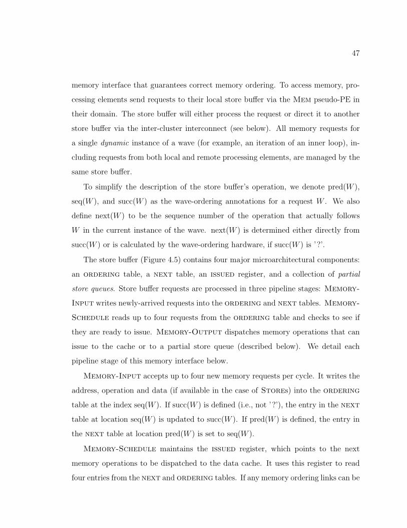
47
memory interface that guarantees correct memory ordering. To access memory, pro-
cessing elements send requests to their local store bu↵er via the Mem pseudo-PE in
their domain. The store bu↵er will either process the request or direct it to another
store bu↵er via the inter-cluster interconnect (see below). All memory requests for
a single dynamic instance of a wave (for example, an iteration of an inner loop), in-
cluding requests from both local and remote processing elements, are managed by the
same store bu↵er.
To simplify the description of the store bu↵er’s operation, we denote pred(W ),
seq(W ), and succ(W ) as the wave-ordering annotations for a request W . We also
define next(W ) to be the sequence number of the operation that actually follows
W in the current instance of the wave. next(W ) is determined either directly from
succ(W ) or is calculated by the wave-ordering hardware, if succ(W ) is ’?’.
The store bu↵er (Figure 4.5) contains four major microarchitectural components:
an ordering table, a next table, an issued register, and a collection of partial
store queues. Store bu↵er requests are processed in three pipeline stages: Memory-
Input writes newly-arrived requests into the ordering and next tables. Memory-
Schedule reads up to four requests from the ordering table and checks to see if
they are ready to issue. Memory-Output dispatches memory operations that can
issue to the cache or to a partial store queue (described below). We detail each
pipeline stage of this memory interface below.
Memory-Input accepts up to four new memory requests per cycle. It writes the
address, operation and data (if available in the case of Stores) into the ordering
table at the index seq(W ). If succ(W ) is defined (i.e., not ’?’), the entry in the next
table at location seq(W ) is updated to succ(W ). If pred(W ) is defined, the entry in
the next table at location pred(W ) is set to seq(W ).
Memory-Schedule maintains the issued register, which points to the next
memory operations to be dispatched to the data cache. It uses this register to read
four entries from the next and ordering tables. If any memory ordering links can be

48
formed (i.e., next table entries are not empty), the memory operations are dispatched
to Memory-Output and the issued register is advanced. The store bu↵er supports
the decoupling of store-data from store addresses as described in Section 3.4.4. This
is done with a hardware structure called a partial store queue, described below. The
salient point for Memory-Schedule, however, is that Stores are sent to Memory-
Output even if their data has not yet arrived.
Partial store queues (see Section 3.4.4) take advantage of the fact that store ad-
dresses can arrive significantly before their data. In these cases, a partial store queue
stores all operations to the same address. These operations must wait for the data
to arrive, but other operations may proceed. When the data finally arrives all, the
operations in the partial store queue can be applied in quick succession. The store
bu↵er contains two partial store queues.
Memory-Output reads and processes dispatched memory operations. Four sit-
uations can occur. (1) The operation is a Load or a Store with its data is present:
The operation proceeds to the data cache. (2) The operation is a Load or a Store
and a partial store queue exists for its address: The memory operation is sent to
the partial store queue. (3) The memory operation is a Store, its data has not yet
arrived, and no partial store queue exists for its address: A free partial store queue is
allocated and the Store is sent to it. (4) The operation is a Load or a Store, but
no free partial store queue is available or the partial store queue is full: The operation
is discarded and the issued register is rolled back. The operation will reissue later.
4.4.1 Routing memory requests
A single store bu↵er must handle all the memory requests for a single wave, but the
memory instructions that produce the requests might execute anywhere in the array
of processing elements. To ensure that requests find their way to the correct store
bu↵er, the WaveScalar hardware maintains a map of wave numbers to store bu↵ers.
When a memory instruction fires, it sends its request to the store bu↵er in the
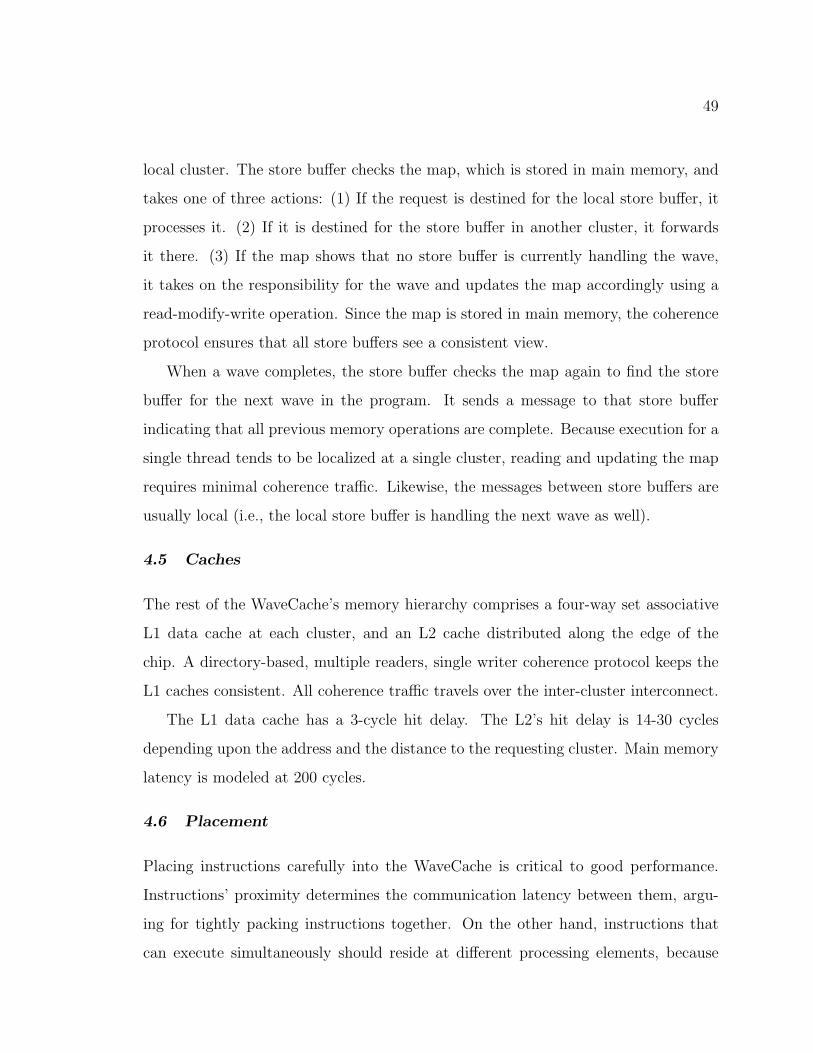
49
local cluster. The store bu↵er checks the map, which is stored in main memory, and
takes one of three actions: (1) If the request is destined for the local store bu↵er, it
processes it. (2) If it is destined for the store bu↵er in another cluster, it forwards
it there. (3) If the map shows that no store bu↵er is currently handling the wave,
it takes on the responsibility for the wave and updates the map accordingly using a
read-modify-write operation. Since the map is stored in main memory, the coherence
protocol ensures that all store bu↵ers see a consistent view.
When a wave completes, the store bu↵er checks the map again to find the store
bu↵er for the next wave in the program. It sends a message to that store bu↵er
indicating that all previous memory operations are complete. Because execution for a
single thread tends to be localized at a single cluster, reading and updating the map
requires minimal coherence tra�c. Likewise, the messages between store bu↵ers are
usually local (i.e., the local store bu↵er is handling the next wave as well).
4.5 Caches
The rest of the WaveCache’s memory hierarchy comprises a four-way set associative
L1 data cache at each cluster, and an L2 cache distributed along the edge of the
chip. A directory-based, multiple readers, single writer coherence protocol keeps the
L1 caches consistent. All coherence tra�c travels over the inter-cluster interconnect.
The L1 data cache has a 3-cycle hit delay. The L2’s hit delay is 14-30 cycles
depending upon the address and the distance to the requesting cluster. Main memory
latency is modeled at 200 cycles.
4.6 Placement
Placing instructions carefully into the WaveCache is critical to good performance.
Instructions’ proximity determines the communication latency between them, argu-
ing for tightly packing instructions together. On the other hand, instructions that
can execute simultaneously should reside at di↵erent processing elements, because

50
competition for the single functional unit will serialize them.
We continue to investigate the placement problem, and details of our endeavors
are available in [43]. Here, we describe the approach we used for the studies in this
thesis.
The placement scheme has a static and a dynamic component. At compile time,
the compiler performs a pre-order, depth-first traversal of the dataflow graph of each
function to generate a linear ordering of the instructions. We chose this traversal,
because it tends to make chains of dependent instructions in the dataflow graph appear
consecutively in the ordering. The compiler breaks the sequence of instructions into
short segments. We tune the segment length for each application.
At runtime, the WaveCache loads these short segments of instructions when an
instruction in a segment that is not mapped into the WaveCache needs to execute. The
entire segment is mapped to a single PE. Because of the ordering the compiler used
to generate the segments, they will usually be dependent on one another. As a result,
they will not compete for execution resources, but instead will execute on consecutive
cycles. The algorithm fills all the PEs in a domain, and then all the domains in a
cluster, before moving on to the next cluster. It fills clusters by “snaking” across the
grid, moving from left to right on the even rows and right to left on the odd rows.
4.7 Managing parallelism
Our placement scheme does a good job of scheduling execution and communication
resources, but a third factor, the so-called “parallelism explosion”, can have a strong
e↵ect on performance in dataflow systems. Parallelism explosion occurs when part of
an application (e.g., the index computation of an inner loop) runs ahead of the rest
of program, generating a vast number of tokens that will not be consumed for a long
time. These tokens overflow the matching table and degrade performance as they
spill to memory. We use a well-known dataflow technique, k-loop bounding [15], to
restrict the number iterations that can be executing at one time to k. We tune k for
51
each application.
52
Chapter 5
RUNNING MULTIPLE THREADS IN WAVESCALAR
The WaveScalar architecture described so far can support a single executing
thread. Modern applications, such as databases and web servers, use multiple threads
both as a useful programming abstraction and to increase performance by exposing
parallelism.
Recently, manufacturers have begun placing several processors on a single die to
create chip multiprocessors (CMPs). There are two reasons for this move: First, scal-
ing challenges will make designing ever-larger superscalar processors infeasible. Sec-
ond, commercial workloads are often more concerned with the aggregate performance
of many threads rather than single-thread performance. Any architecture intended
as an alternative to CMPs must be able to execute multiple threads simultaneously.
This section extends the single-threaded WaveScalar design to execute multiple
threads. The key issues we must address to allow WaveScalar to execute multiple
threads are managing multiple, parallel sequences of wave-ordered memory operations,
di↵erentiating between data values that belong to di↵erent threads, and allowing
threads to communicate. WaveScalar’s solution to these problems are all simple
and e�cient. For instance, WaveScalar is the first architecture to allow programs
to manage memory ordering directly by creating and destroying memory orderings
and dynamically binding them to a particular thread. WaveScalar’s thread-spawning
facility is e�cient enough to parallelize small loops. Its synchronization mechanism
is also light-weight and tightly integrated into the dataflow framework.
The required changes to the WaveCache to support the ISA extensions are surpris-
ingly small, and they do not impact the overall structure of the WaveCache, because
53
executing threads dynamically share most WaveCache processing resources.
The next two sections describe the multihthreading ISA extensions, then we dis-
cuss the changes needed to the hardware.
5.1 Multiple memory orderings
As previously introduced, the wave-ordered memory interface provides support for a
single memory ordering. Forcing all threads to contend for the same memory inter-
face, even if it were possible, would be detrimental to performance. Consequently, to
support multiple threads, we extend the WaveScalar instruction set to allow multiple
independent sequences of ordered memory accesses, each of which belongs to a sep-
arate thread. First, we annotate every data value with a Thread-Id in addition to
its Wave-Number. Then, we introduce instructions to associate memory-ordering
resources with particular Thread-Ids.
Thread-Ids The WaveCache already has a mechanism for distinguishing values
and memory requests within a single thread from one another – they are tagged
with Wave-Numbers. To di↵erentiate values from di↵erent threads, we extend this
tag with a Thread-Id and modify WaveScalar’s dataflow firing rule to require that
operand tags match on both Thread-Id and Wave-Number. As with Wave-
Numbers, additional instructions are provided to directly manipulate Thread-Ids.
In figures and examples throughout the rest of this thesis, the notation <t, w>.d
signifies a token tagged with Thread-Id t and Wave-Number w and having data
value d.
To manipulate Thread-Ids and Wave-Numbers, we introduce several instruc-
tions that convert Wave-Numbers and Thread-Ids to normal data values and
back again. The most powerful of these is Data-To-Thread-Wave, which sets
both the Thread-Id and Wave-Number at once; Data-To-Thread-Wave takes
three inputs, <t0
, w0
>.t1
, <t0
, w0
>.w1
, and <t0
, w0
>.d and produces as output
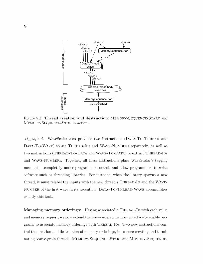
54
<t:w>.u
MemorySequenceStart
<t:w>.s <t:w>.u<t:w>.d
<t:w>.e<t:w>.f
MemorySequenceStop
Ordered thread body executes
<s:u>.finished
Th
rea
d c
rea
tion
Thre
ad
destru
ctio
n
DataToThreadWave
<s:u>.e<s:u>.d
<s:u>.f
Figure 5.1: Thread creation and destruction: Memory-Sequence-Start andMemory-Sequence-Stop in action.
<t1
, w1
>.d. WaveScalar also provides two instructions (Data-To-Thread and
Data-To-Wave) to set Thread-Ids and Wave-Numbers separately, as well as
two instructions (Thread-To-Data and Wave-To-Data) to extract Thread-Ids
and Wave-Numbers. Together, all these instructions place WaveScalar’s tagging
mechanism completely under programmer control, and allow programmers to write
software such as threading libraries. For instance, when the library spawns a new
thread, it must relabel the inputs with the new thread’s Thread-Id and the Wave-
Number of the first wave in its execution. Data-To-Thread-Wave accomplishes
exactly this task.
Managing memory orderings: Having associated a Thread-Id with each value
and memory request, we now extend the wave-ordered memory interface to enable pro-
grams to associate memory orderings with Thread-Ids. Two new instructions con-
trol the creation and destruction of memory orderings, in essence creating and termi-
nating coarse-grain threads: Memory-Sequence-Start and Memory-Sequence-
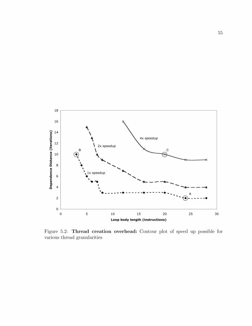
55
A
B C
0
2
4
6
8
10
12
14
16
18
0 5 10 15 20 25 30
Loop body length (instructions)
Dep
en
den
ce D
ista
nce (
iterati
on
s)
4x speedup
2x speedup
1x speedup
Figure 5.2: Thread creation overhead: Contour plot of speed up possible forvarious thread granularities
56
Stop.
Memory-Sequence-Start creates a new wave-ordered memory sequence for a
new thread. This sequence is assigned to a store bu↵er, which services all memory
requests tagged with the thread’s Thread-Id and Wave-Number; requests with
the same Thread-Id but a di↵erent Wave-Number cause a new store bu↵er to be
allocated.
Memory-Sequence-Stop terminates a memory ordering sequence. The wave-
ordered memory system uses this instruction to ensure that all memory operations in
the sequence have completed before its store bu↵er resources are released.
Figure 5.1 illustrates how to use these two instructions to create and destroy a
thread. Thread t spawns a new thread s by sending s’s Thread-Id (s) and Wave-
Number (u) to Memory-Sequence-Start, which allocates a store bu↵er to han-
dle the first wave in the new thread. The result of the Memory-Sequence-Start
instruction triggers the three Data-To-Thread-Wave instructions that set up s’s
three input parameters. The inputs to each Data-To-Thread-Wave instruction are
a parameter value (d, e, or f), the new Thread-Id (s) and the new Wave-Number
(u). A token with u is produced by Memory-Sequence-Start deliberately, to guar-
antee that no instructions in thread s execute until Memory-Sequence-Start has
finished allocating its store bu↵er. Thread s terminates with Memory-Sequence-
Stop, whose output token <s, u>.finished guarantees that its store bu↵er area has
been deallocated.
Implementation Adding support for multiple memory orderings requires only small
changes to the WaveCache’s microarchitecture. First, the widths of the communica-
tion busses and operand queues must be expanded to hold Thread-Ids. Second,
instead of storing each static instruction from the working set of a program in the
WaveCache, one copy of each static instruction is stored for each thread. This means
that if two threads are executing the same static instructions, each may map the static
57
instructions to di↵erent PEs. Finally, the PEs must implement the Thread-Id and
Wave-Number manipulation instructions.
E�ciency The overhead associated with spawning a thread directly a↵ects the
granularity of extractable parallelism. To assess this overhead in the WaveCache, we
designed a controlled experiment consisting of a simple parallel loop in which each
iteration executes in a separate thread. The threads have their own wave-ordered
memory sequences but do not have private stacks, so they cannot make function
calls.
We varied the size of the loop body, which a↵ects the granularity of parallelism,
and the dependence distance between memory operands, which a↵ects the number
of threads that can execute simultaneously. We then measured speedup compared
to a serial execution of a loop doing the same work. The experiment’s goal is to
answer the following question: Given a loop body with a critical path length of N
instructions and a dependence distance that allows T iterations to run in parallel,
can the WaveCache speed up execution by spawning a new thread for every loop
iteration?
Figure 5.2 is a contour plot of speedup of the loop as a function of its loop size
(critical path length in Add instructions, the horizontal axis) and dependence distance
(independent iterations, the vertical axis). Contour lines are shown for speedups of 1⇥
(no speedup), 2⇥ and 4⇥. The area above each line is a region of program speedup at
or above the labeled value. The data show that the WaveScalar overhead of creating
and destroying threads is so low that for loop bodies of only 24 dependent instructions
and a dependence distance of 3, it becomes advantageous to spawn a thread to execute
each iteration (‘A’ in the figure). A dependence distance of 10 reduces the size of
profitably parallelizable loops to only 4 instructions (‘B’). Increasing the number of
instructions to 20 quadruples performance (‘C’).
58
5.2 Synchronization
The ability to e�ciently create and terminate pthread-style threads, as described in
the previous section, provides only part of the functionality required to make multi-
threading useful. Independent threads must also synchronize and communicate with
one another. To this end, WaveScalar provides a memory fence instruction that allows
WaveScalar to enforce a relaxed consistency model and a specialized instruction that
models a hardware queue lock.
5.2.1 Memory fence
Wave-ordered memory provides a single thread with a consistent view of memory,
since it guarantees that the results of earlier memory operations are visible to later
operations. In some situations, such as before taking or releasing a lock, a multi-
threaded processor must guarantee that the results of a thread’s memory operations
are visible to other threads. We add to the ISA an additional instruction, Memory-
Nop-Ack that provides this assurance by acting as a memory fence. Memory-
Nop-Ack prompts the wave-ordered interface to commit the thread’s prior loads
and stores to memory, thereby ensuring their visibility to other threads and providing
WaveScalar with a relaxed consistency model [4]. The interface then returns an
acknowledgment, which the thread can use to trigger execution of its subsequent
instructions.
5.2.2 Interthread synchronization
Most commercially deployed multiprocessors and multi-threaded processors provide
interthread synchronization through the memory system via primitives such as test-
and-set, compare-and-swap, or load-lock/store-conditional. Some re-
search e↵orts also propose building complete locking mechanisms in hardware [27, 62].
Such queue locks o↵er many performance advantages in the presence of high lock con-

59
tention.
In WaveScalar, we add support for queue locks in a way that constrains neither the
number of locks nor the number of threads that may contend for the lock. This support
is embodied in a synchronization instruction called Thread-Coordinate, which
synchronizes two threads by passing a value between them. Thread-Coordinate
is similar in spirit to other lightweight synchronization primitives [34, 11], but is
tailored to WaveScalar’s execution model.
As Figure 5.3 illustrates, Thread-Coordinate requires slightly di↵erent match-
ing rules1. All WaveScalar instructions except Thread-Coordinate fire when the
tags of two input values match, and they produce outputs with the same tag (Fig-
ure 5.3, left). For example, in the figure, both the input tokens and the result have
Thread-Id t0
and Wave-Number w0
.
In contrast, Thread-Coordinate fires when the data value of a token at its
first input matches the Thread-Id of a token at its second input. This is depicted
on the right side of Figure 5.3, where the data value of the left input token and the
Thread-Id of the right input token are both t1
. Thread-Coordinate generates
an output token with the Thread-Id and Wave-Number from the first input and
the data value from the second input. In Figure 5.3, this produces an output of
<t0
, w0
>.d. In essence, Thread-Coordinate passes the second input’s value (d)
to the thread of the first input (t0
). Since the two inputs come from di↵erent threads,
this forces the receiving thread (t0
in this case) to wait for the data from the sending
thread (t1
) before continuing execution.
To support Thread-Coordinate in hardware, we augment the tag match-
ing logic at each PE. We add two counters at each PE, one for each input to a
Thread-Coordinate instruction. When an input arrives, the PE replaces its
1Some previous dataflow machines altered the dataflow firing rule for other purposes. For ex-ample, Sigma-1 used “sticky” tags to prevent the consumption of loop-invariant data and “error”tokens to swallow values of instructions that incurred exceptions [55]. Monsoon’s M-structurestore units had a special matching rule to enforce load-store order [51].
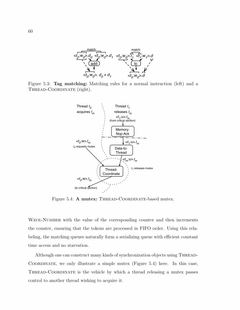
60
tc
matchmatch
add
<t0:w0>. d0 + d1
<t0:w0>.d1<t0:w0>.d0
<t0:w0>.d
<t1:w1>.d<t0:w0>.t1
Figure 5.3: Tag matching: Matching rules for a normal instruction (left) and aThread-Coordinate (right).
<tm:u>.tm
Thread-
Coordinate
Data-to-
Thread
releases tmacquires tm
<t1:u>.tm
<t0:w>.tm
Memory-
Nop-Ack
<t1:u>.tm(from critical section)
<t0:w>.tm
(to critical section)
Thread t0 Thread t1
t1 releases mutex
t0 requests mutex
Figure 5.4: A mutex: Thread-Coordinate-based mutex.
Wave-Number with the value of the corresponding counter and then increments
the counter, ensuring that the tokens are processed in FIFO order. Using this rela-
beling, the matching queues naturally form a serializing queue with e�cient constant
time access and no starvation.
Although one can construct many kinds of synchronization objects using Thread-
Coordinate, we only illustrate a simple mutex (Figure 5.4) here. In this case,
Thread-Coordinate is the vehicle by which a thread releasing a mutex passes
control to another thread wishing to acquire it.
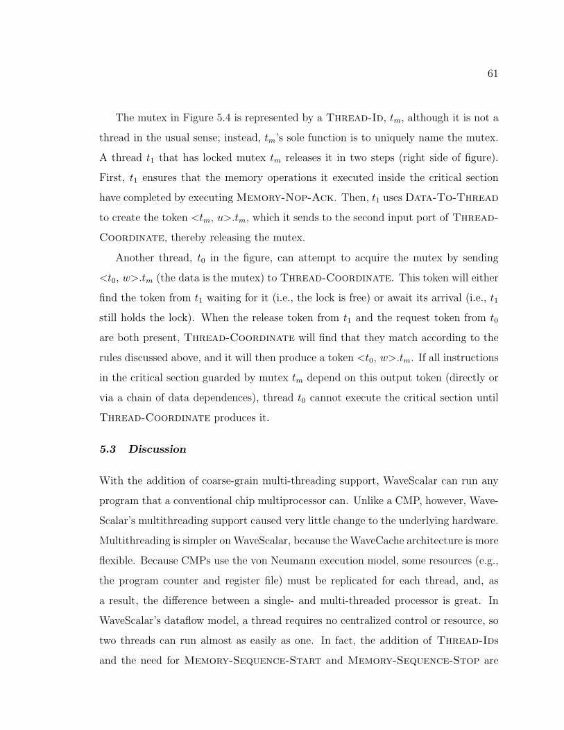
61
The mutex in Figure 5.4 is represented by a Thread-Id, tm, although it is not a
thread in the usual sense; instead, tm’s sole function is to uniquely name the mutex.
A thread t1
that has locked mutex tm releases it in two steps (right side of figure).
First, t1
ensures that the memory operations it executed inside the critical section
have completed by executing Memory-Nop-Ack. Then, t1
uses Data-To-Thread
to create the token <tm, u>.tm, which it sends to the second input port of Thread-
Coordinate, thereby releasing the mutex.
Another thread, t0
in the figure, can attempt to acquire the mutex by sending
<t0
, w>.tm (the data is the mutex) to Thread-Coordinate. This token will either
find the token from t1
waiting for it (i.e., the lock is free) or await its arrival (i.e., t1
still holds the lock). When the release token from t1
and the request token from t0
are both present, Thread-Coordinate will find that they match according to the
rules discussed above, and it will then produce a token <t0
, w>.tm. If all instructions
in the critical section guarded by mutex tm depend on this output token (directly or
via a chain of data dependences), thread t0
cannot execute the critical section until
Thread-Coordinate produces it.
5.3 Discussion
With the addition of coarse-grain multi-threading support, WaveScalar can run any
program that a conventional chip multiprocessor can. Unlike a CMP, however, Wave-
Scalar’s multithreading support caused very little change to the underlying hardware.
Multithreading is simpler on WaveScalar, because the WaveCache architecture is more
flexible. Because CMPs use the von Neumann execution model, some resources (e.g.,
the program counter and register file) must be replicated for each thread, and, as
a result, the di↵erence between a single- and multi-threaded processor is great. In
WaveScalar’s dataflow model, a thread requires no centralized control or resource, so
two threads can run almost as easily as one. In fact, the addition of Thread-Ids
and the need for Memory-Sequence-Start and Memory-Sequence-Stop are
62
both results of WaveScalar’s need to support von Neumann-style memory semantics.
They would not be needed in a pure dataflow system.
The next two chapters describe our experimental infrastructure, evaluate the mul-
tithreaded WaveCache, and demonstrate that it achieves both superior e�ciency and
performance compared to von Neumann processors. Chapter 8 takes WaveScalar be-
yond the constraints of von Neumann execution and demonstrates the power of its
dataflow execution model.
63
Chapter 6
EXPERIMENTAL INFRASTRUCTURE
This chapter describes the experimental infrastructure we use to evaluate the
WaveScalar architecture described in Chapters 7 and 8. There are three key tools: A
synthesizable RTL model and the accompanying synthesis tools, a WaveScalar tool
chain that includes a cycle-level architectural simulator, and a set of workloads that
span a wide range of di↵erent applications.
In then next two chapters we will use these tools to search the space of WaveScalar
processor designs and compare the best designs to contemporary single-threaded and
multi-threaded processors. We describe each of the tools in turn.
6.1 The RTL model
Since WaveScalar is a tiled dataflow processor, it is di↵erent enough from conventional
von Neumann processors that we cannot draw on past research, existing tools, or
industrial experience to understand area and cycle-time requirements. Since these
parameters are crucial for determining how well WaveScalar performs and how to
partition the silicon resources, we constructed a synthesizable RTL model of the
components described in Chapters 4 and 5.
The synthesizable RTL model is written in Verilog, and targets a 90nm ASIC
implementation. Considerable e↵ort was put into designing, and redesigning this
Verilog to be both area-e�cient and fast. The final clock speed (22 FO4) comes from
our fourth major redesign.
The 90nm process is the most current process technology available, so the results
presented here should scale well to future technologies. In addition to using a modern
64
process, we performed both front-end and back-end synthesis to get as realistic a
model as possible. The model makes extensive use of Synopsys DesignWare IP [2]
for critical components such as SRAM controllers, queue controllers, arbiters, and
arithmetic units. The design currently uses a single frequency domain and a single
voltage domain, but the tiled and hierarchical architecture would lend itself easily to
multiple voltage and frequency domains in the future.
6.1.1 ASIC design flow
We used the most up-to-date tools available for Verilog synthesis. Synopsys VCS
provided RTL simulation and functional verification of the post-synthesis netlists.
Front-end synthesis was done using Synopsys DesignCompiler. Cadence FirstEn-
counter handled back-end synthesis tasks such as floorplanning, clock-tree synthesis,
and place and route [1]. By using back-end synthesis, the area and timing results
presented here include realistic physical e↵ects, such as incomplete core utilization
and wire delay, that are critical for characterizing design performance at 90nm and
below.
6.1.2 Standard cell libraries
Our design uses the 90nm high-performance GT standard cell libraries from Taiwan
Semiconductor Manufacturing Company (TSMC) [3]. The library contains three im-
plementations of cells, each with a di↵erent threshold voltage, for balancing power
and speed. We allow DesignCompiler and FirstEncounter to pick the appropriate cell
implementation for each path.
The memory in our design is a mixture of SRAM memories generated from a
commercial memory compiler (used for the large memory structures, such as data
caches) and Synopsys DesignWare IP memory building blocks (used for smaller mem-
ory structures).

65
6.1.3 Timing data
Architects commonly measure clock cycle time in a process-independent metric, fanout-
of-four (FO4). A design’s cycle time in FO4 does not change (much) as the fabrica-
tion process changes, thus enabling a more direct comparison of designs across process
technologies.
Synthesis tools, however, report delay in absolute terms (nanoseconds). To convert
nanoseconds to FO4, we followed academic precedent [61] and used the technique
suggested in [14] to measure the absolute delay of one FO4. We synthesized a ring
oscillator using the same design flow and top-speed standard cells (LVT) used in our
design and measured FO1 (13.8ps). We then multiplied this delay by three to yield
an approximation of one FO4 (41.4ps). All timing data presented here is reported in
FO4 based upon this measurement.
6.2 The WaveScalar tool chain
We use a binary translator-based tool chain to create WaveScalar executables. Fig-
ure 6.1 shows the components of the system and how they interact. Three components,
the binary translator, the performance simulator, and the placement system, are most
important. We address the translator and simulator here. Section 4.6 describe the
placement algorithm we use.
6.2.1 The binary translator
The binary translator converts Alpha AXP binaries into WaveScalar assembly lan-
guage. There are two key tasks the translator must accomplish: First, it converts the
von Neumann style control structures (branches, PC-based function calls, etc.) into
dataflow constructs. Second, it breaks the program into waves and adds annotations
that allow the wave-ordered memory system to enforce the correct memory ordering.

66
Dec CC compiler
Binary translator Hand-coding
Assembler
Functional simulator (profiling)
Placement
Performance simulation
AXP Binary
WS assembly WS assembly
WS Binary
WS Binary
Profile
Placement
C code
Figure 6.1: The WaveScalar tool chain: The tool chain we use to compile andexecute WaveScalar programs.
67
Control
In von Neumann systems, the program counter controls execution. Branches and
function calls manipulate the program counter to steer execution along the correct
path in the program. WaveScalar uses the Steer instruction (see Chapter 2) to guide
execution instead.
Replacing PC-based conditional branch instructions with Steer instructions re-
quires inserting one Steer instruction for each of the 64 registers the Alpha ISA
defines at each branch point. This results in a very large number of Steer instruc-
tions, and the binary translator uses several techniques, including control dependence
analysis and dead value analysis, to optimize away as many of them as possible.
The binary translator uses the Indirect-Send instruction to implement register-
indirect jumps and function calls as described in Chapter 2.
Wave creation
To support wave-ordered memory (Chapter 3), the translator must break each func-
tions into a series of waves. Chapter 3 defines precisely the properties that a wave
must have, but the binary translator generates waves that satisfy a simpler set of
properties: It produces waves that have a single entrance, only contain function calls
at wave exits, and contain no back edges.
To break up a function, the translator uses control analysis to label back edges in
the control flow graph. Then it uses the entrance block of the function as the entrance
of the first wave. The translator expands that wave using a breadth-first traversal of
the control flow graph. It stops the wave’s growth along a path when it encounters a
function call or a basic block with a back edge entering or leaving it. Once the first
wave has stopped growing, the translator selects one of the points at which it stopped
and starts a new wave with that basic block.
To assign predecessor, successor, sequence, and ripple numbers, the translator
68
traverses each wave in depth-first order and assigns or updates those annotations as
necessary.
Limitations
The binary translator was written for two reasons: First it provided an expedient path
to generating a WaveScalar executable from C code. Second, it demonstrates that
building a von Neumann-to-dataflow translator is possible, laying the groundwork for
a smoother transition between the two execution models.
The approach su↵ers from several limitations, however. First, using Alpha binaries
as the input to the translator severely restricts the optimizations that the binary
translator can perform. For instance, alias analysis is e↵ectively impossible, because
no high-level information about memory use is available. The DEC compiler partially
compensates for this limitation, since it provides good control over many optimizations
that are useful in WaveScalar compilation (e.g., function inlining and loop unrolling).
Second, the binary translator cannot handle irreducible loops (usually the result
of gotos), jump-table-based switch statements, or compiler intrinsics that do not
follow the Alpha calling convention. These limitations are strictly a deficiency of our
translator, not a limitation of WaveScalar’s ISA or execution model. In practice, we
restructure the source code to eliminate these constructs, if possible.
Our group is currently working on a full-fledged WaveScalar compiler that will ad-
dress all of these shortcomings and provide the foundation a more detailed exploration
of WaveScalar compilation.
6.2.2 The performance simulator
To measure WaveScalar performance we use a cycle-level processor simulator. The
simulator is very detailed and models all the components of the architecture including
the pipelined PE, the wave-ordered store bu↵er, the network switch, the memory hier-
archy, and all the interconnects that connect these components. It also answers basic
69
questions, such as how the sizing of microarchitectural features a↵ect performance.
We use a set of microbenchmarks to check that the simulator’s timing and behavior
are correct along with a set of larger regression tests that ensure application-level
correctness.
The simulator also provides emulation for the operating system by providing im-
plementations of the necessary system calls. It also emulates some features that a
WaveScalar operating system would provide. For instance, the simulator handles the
dynamic portion of the instruction placement process and accounts for an approxi-
mation of the delay it would incur.
To make measurements comparable with conventional architectures, we measure
performance in alpha instructions per cycle (AIPC) and base our superscalar com-
parison on a machine with similar clock speed [32]. AIPC measures the number of
non-overhead instructions (i.e., instructions other than Steer, �, etc.) executed per
cycle. The AIPC measurements for the superscalar architectures we compare to are
in good agreement with other measurements [45].
6.3 Applications
We used three groups of workloads to evaluate the WaveScalar processor. Each fo-
cuses on a di↵erent aspect of WaveScalar performance. To measure single-threaded
performance, we chose a selection of the Spec2000 [58] benchmark suite (ammp, art,
equake, gzip, twolf and mcf ). To evaluate the processor’s media processing perfor-
mance we use rawdaudio, mgeg2encode, and djpeg from Mediabench [38]. Finally,
we use six of the Splash2 [6] benchmarks, ↵t, lu-continuous, ocean-noncontinuous,
raytrace, water-spatial, and radix, to explore multi-threaded performance.
We compiled each application with the DEC cc compiler using -O4 -fast -inline
speed optimizations. A binary translator-based tool chain was used to convert these
binaries into WaveScalar assembly and then into WaveScalar binaries. The choice
of benchmarks represents a range of applications as well as the limitations of our
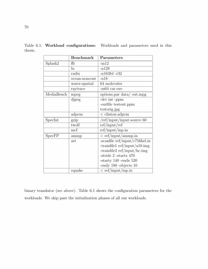
70
Table 6.1: Workload configurations: Workloads and parameters used in thisthesis.
Benchmark Parameters
Splash2 ↵t -m12lu -n128radix -n16384 -r32ocean-noncont -n18water-spatial 64 moleculesraytrace -m64 car.env
MediaBench mpeg options.par data/ out.mpgdjpeg -dct int -ppm
-outfile testout.ppmtestorig.jpg
adpcm < clinton.adpcm
SpecInt gzip /ref/input/input.source 60twolf ref/input/refmcf ref/input/inp.in
SpecFP ammp < ref/input/ammp.inart -scanfile ref/input/c756hel.in
-trainfile1 ref/input/a10.img-trainfile2 ref/input/hc.img-stride 2 -startx 470-starty 140 -endx 520-endy 180 -objects 10
equake < ref/input/inp.in
binary translator (see above). Table 6.1 shows the configuration parameters for the
workloads. We skip past the initialization phases of all our workloads.

71
Chapter 7
WAVECACHE PERFORMANCE
Chapters 2-5 described WaveScalar’s single- and multi-threaded instruction set
and presented the WaveCache processor design. The WaveCache design defines a
spectrum of processor configurations. At one end of the spectrum is a small Wave-
Cache processor, comprising just a single cluster, which would be suitable for small,
single-threaded or embedded applications. At the other end, a supercomputer proces-
sor might contain tens of clusters and hundreds or thousands of processing elements.
The ability to move easily along this design continuum is a key objective of tiled
architectures. A second objective is that they be able to tolerate such drastic changes
in area by localizing data communication, thereby reducing latency. This section
explores how well the WaveScalar architecture performs while achieving these goals.
We begin in Section 7.1 with a detailed look at the area budget of a particular
WaveScalar processor configuration. Then, to understand a larger design space, Sec-
tion 7.2 uses data from our RTL synthesis to develop an area model that describes the
area requirements for a range of designs. We use the resulting model to enumerate
a large class of WaveScalar processor designs that could be built in modern process
technology. We evaluate these designs using our suite of single- and multi-threaded
workloads and use the results to perform an area/performance pareto analysis of
the WaveScalar design space covered by our RTL design and area model. Lastly, in
Section 7.3, we examine changes in the network tra�c patterns as the size of the
WaveScalar processor increases.

72
Tab
le7.
1:A
clust
er’s
are
abudget
:A
bre
akdow
nof
the
area
requ
ired
for
asi
ngl
ecl
ust
er.
Are
ain
PE
Are
ain
Dom
ain
Are
ain
Clu
ster
%of
PE
%of
Dom
ain
%of
Clu
ster
PE
Input
0.01
mm
2
0.09
mm
2
0.37
mm
2
1.2%
1.1%
0.9%
Match
0.58
mm
2
4.60
mm
2
18.4
1mm
2
61.0
%55
.2%
43.3
%D
ispa
tch
0.01
mm
2
0.05
mm
2
0.18
mm
2
0.6%
0.6%
0.4%
Execute
0.02
mm
2
0.19
mm
2
0.77
mm
2
2.5%
2.3%
1.8%
Output
0.02
mm
2
0.14
mm
2
0.55
mm
2
1.8%
1.7%
1.3%
inst
ruct
ion
stor
e0.
31m
m2
2.47
mm
2
9.88
mm
2
32.8
%29
.6%
23.2
%to
tal
0.94
mm
2
7.54
mm
2
30.1
6mm
2
100%
90.5
%71
.0%
Dom
ain
Mem
PE
0.13
mm
2
0.53
mm
2
1.6%
1.2%
Net
PE
0.13
mm
2
0.53
mm
2
1.6%
1.2%
8⇥P
E7.
54m
m2
30.1
6mm
2
90.5
%71
.0%
FP
U0.
53m
m2
2.11
mm
2
6.3%
5.0%
tota
l8.
33m
m2
33.3
2mm
2
100%
78.4
%C
lust
er4⇥
dom
ain
33.3
2mm
2
78.4
%ne
twor
ksw
itch
0.37
mm
2
0.9%
stor
ebu
↵er
2.62
mm
2
6.2%
data
cach
e6.
18m
m2
14.5
%to
tal
42.5
0mm
2
100.
0%

73
7.1 Area model and timing results
Our RTL toolchain provides both area and delay values for each component of the
WaveScalar processor. For this study, we restrict ourselves to processors that achieve
a clock rate of 22 FO4, which occurs for a wide range of designs in our Verilog
model. This is the shortest cycle time allowed by the critical path within the PE.
For most configurations, the critical path is through the execution unit when using
operands from the other PE in the pod. However, enlarging the matching cache or
instruction cache memory structures beyond 256 entries makes paths in the Match
and Dispatch stages critical paths. Floating point units are pipelined to avoid
putting floating-point execution on the critical path. Input and Output devote 9
and 5 FO4, respectively, to traversing the intra-domain network, so there is no need
for an additional stage for intra-domain wire delay.
Since the critical path is the ALU for designs with smaller than 256-entry matching
caches and 256-entry instruction caches, we can resize these structures downward for
optimum area-performance without dramatically altering the cycle time. This allows
us to evaluate a large number of potential processing element designs based on area
without worrying about an accompanying change in cycle time. We confirmed this by
synthesizing designs with 16- to 256-entry matching caches and with 8- to 256-entry
instruction caches. The clock cycle for these configurations changed by less than 5%
until the structures reached 256 entries, at which point the cycle time increased by
about 21% for the matching cache and 7% for the instruction cache. These latencies
and structure size limits for our study are summarized in Table 7.2 and Table 7.3,
respectively.
Table 7.1 shows how the die area is spent for the baseline design described in
Table 7.2. Note that the 71% of the cluster area is devoted to PEs. Also, almost
all the area, ⇠83%, is spent on SRAM cells which make up the instruction stores,
matching caches, store bu↵er ordering tables, and L1 data caches.
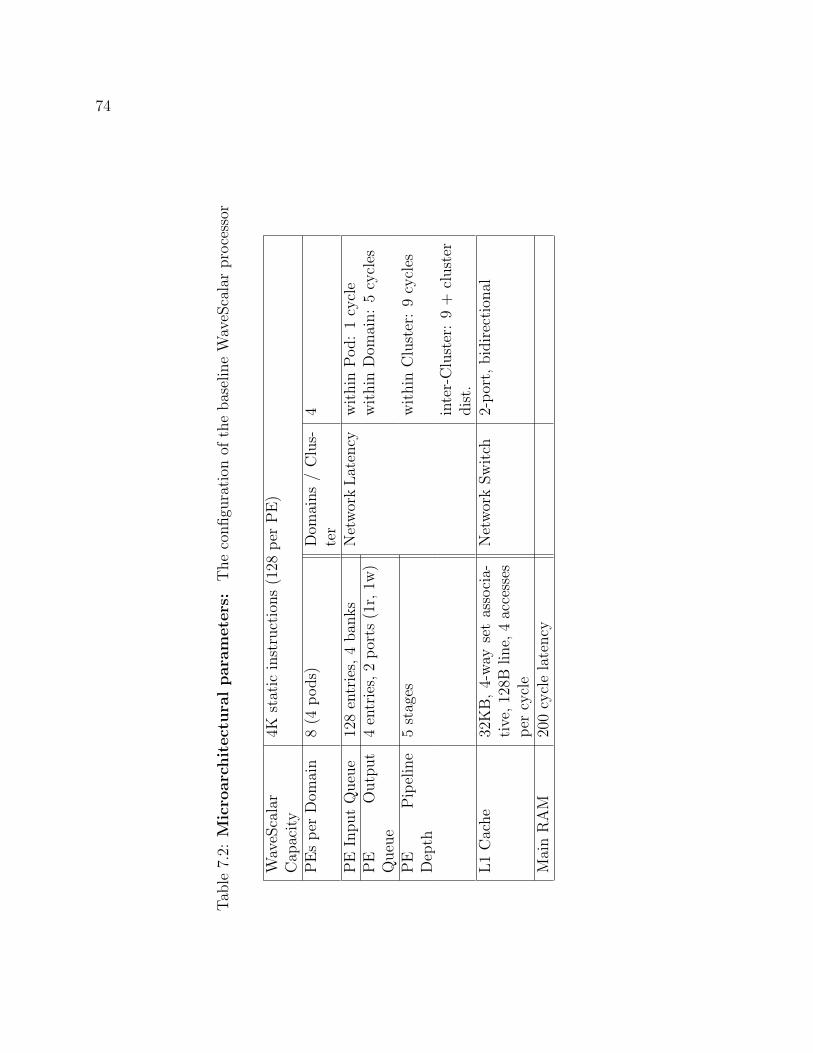
74
Tab
le7.
2:M
icro
arc
hit
ectu
ralpara
met
ers:
The
configu
rati
onof
the
bas
elin
eW
aveS
cala
rpro
cess
or
Wav
eSca
lar
Cap
acity
4Kst
atic
inst
ruct
ions
(128
per
PE
)
PE
sper
Dom
ain
8(4
pod
s)D
omai
ns
/C
lus-
ter
4
PE
Input
Queu
e12
8en
trie
s,4
ban
ksN
etw
ork
Lat
ency
wit
hin
Pod
:1
cycl
eP
EO
utp
ut
Queu
e4
entr
ies,
2por
ts(1
r,1w
)w
ithin
Dom
ain:
5cy
cles
PE
Pip
elin
eD
epth
5st
ages
wit
hin
Clu
ster
:9
cycl
es
inte
r-C
lust
er:
9+
clust
erdis
t.L1
Cac
he
32K
B,
4-w
ayse
tas
soci
a-ti
ve,12
8Bline,
4ac
cess
esper
cycl
e
Net
wor
kSw
itch
2-por
t,bid
irec
tion
al
Mai
nR
AM
200
cycl
ela
tency

75
7.2 Performance analysis
To understand the performance characteristics of our WaveScalar processor design,
we perform a systematic search of the entire design space. Measurements from our
RTL model provide an area model for WaveScalar processors. For both single- and
multi-threaded workloads, we combine the output of the area model with results
from our WaveCache simulator to perform an area-vs-performance pareto analysis of
the WaveScalar design space. Then, we compare the performance of several pareto-
optimal designs to more conventional von Neumann processors in terms of raw per-
formance and area-e�ciency.
7.2.1 The area model
Our area model considers the seven parameters with the strongest e↵ect on the area
requirements. Table 7.3 summarizes these parameters (top half of the table) and how
they combine with data from the RTL model to form the total area, WCarea
(bottom
of the table). For both the matching table and instruction store, we synthesized
versions from 8 to 128 entries to confirm that area varies linearly with capacity. For
the L1 and L2 caches, we used the area of 1KB and 1MB arrays provided by a memory
compiler to perform a similar verification. The “Utilization factor” is the measure
of how densely the tools managed to pack cells together, while still having space for
routing. Multiplying by its inverse accounts for the wiring costs in the entire design.
The area model ignores some minor e↵ects. For instance, it assumes that wiring
costs do not decrease with fewer than four domains in a cluster, thereby overestimating
this cost for small clusters. Nevertheless, the structures accounting for most of the
silicon area (⇠80% as discussed in Section 7.1) are almost exactly represented.
There are three other WaveScalar parameters that a↵ect performance that are not
included in the model because they do not have a large e↵ect on area. These are the
widths of the three levels of WaveScalar interconnect. For this study, we allow one
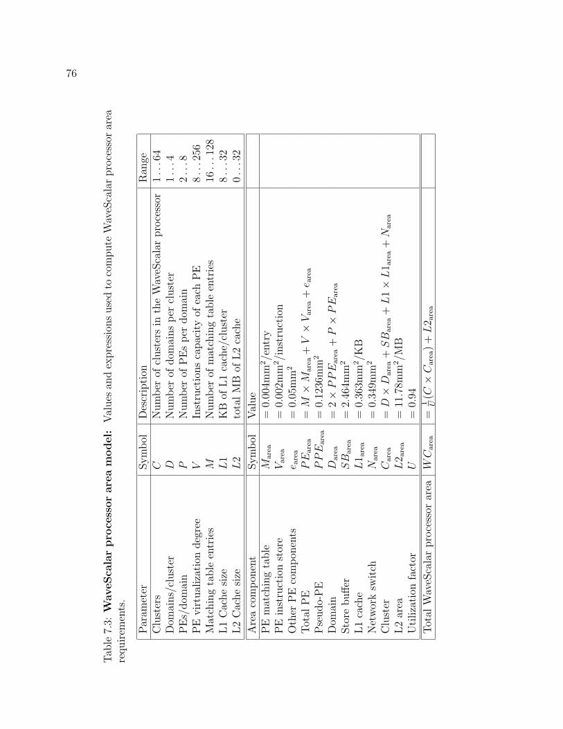
76
Tab
le7.
3:W
aveS
cala
rpro
cess
or
are
am
odel
:Val
ues
and
expre
ssio
ns
use
dto
com
pute
Wav
eSca
lar
pro
cess
orar
eare
quir
emen
ts.
Par
amet
erSym
bol
Des
crip
tion
Ran
geC
lust
ers
CN
um
ber
ofcl
ust
ers
inth
eW
aveS
cala
rpro
cess
or1..
.64
Dom
ains/
clust
erD
Num
ber
ofdom
ains
per
clust
er1..
.4P
Es/
dom
ain
PN
um
ber
ofP
Es
per
dom
ain
2..
.8P
Evi
rtual
izat
ion
deg
ree
VIn
stru
ctio
ns
capac
ity
ofea
chP
E8..
.256
Mat
chin
gta
ble
entr
ies
MN
um
ber
ofm
atch
ing
table
entr
ies
16..
.128
L1
Cac
he
size
L1
KB
ofL1
cach
e/cl
ust
er8..
.32
L2
Cac
he
size
L2
tota
lM
Bof
L2
cach
e0..
.32
Are
aco
mpon
ent
Sym
bol
Val
ue
PE
mat
chin
gta
ble
Marea
=0.
004m
m2
/ent
ryP
Ein
stru
ctio
nst
ore
Varea
=0.
002m
m2
/inst
ruct
ion
Oth
erP
Eco
mpon
ents
e area
=0.
05m
m2
Tot
alP
EP
Earea
=M⇥
Marea
+V⇥
Varea
+e a
rea
Pse
udo-
PE
PP
Earea
=0.
1236
mm
2
Dom
ain
Darea
=2⇥
PP
Earea
+P⇥
PE
area
Sto
rebu↵er
SB
area
=2.
464m
m2
L1
cach
eL
1 area
=0.
363m
m2
/KB
Net
wor
ksw
itch
Narea
=0.
349m
m2
Clu
ster
Carea
=D⇥
Darea
+SB
area
+L
1⇥
L1 a
rea
+N
area
L2
area
L2 a
rea
=11
.78m
m2
/MB
Uti
liza
tion
fact
orU
=0.
94
Tot
alW
aveS
cala
rpro
cess
orar
eaW
Carea
=1 U(C⇥
Carea
)+
L2 a
rea

77
message per cycle, per PE on the intra-domain network, two messages per domain on
the inter-domain network, and two messages per cycle on the network links between
clusters. Adding more bandwidth does not significantly increase performance (less
than 5%), and using a narrower inter-cluster and inter-domain interconnects reduces
the size of a cluster by less than 1%, because the additional wires lay on top of logic
that is already present.
The area model contains parameters that enumerate the range of possible WaveScalar
processor designs. For parameters D (domains per cluster), P (processors per do-
main), V (instructions per PE) and M (matching-table entries), we set the range
to match constraints imposed by the RTL model. As discussed in Section 7.1, in-
creasing any of these parameters past the maximum value impacts cycle time. The
minimum values for M and V reflect restrictions on minimum memory array sizes in
our synthesis toolchain.
The ranges in the table allow for over twenty-one thousand WaveScalar processor
configurations, but many of them are clearly poor, unbalanced designs, while oth-
ers are extremely large (up to 12,000mm2). We can reduce the number of designs
dramatically if we apply some simple rules.
First, we bound the die size at 400mm2 in 90nm to allow for aggressively large yet
feasible designs. Next, we remove designs that are clearly ine�cient. For instance,
it makes no sense to have more than one domain if the design contains fewer than
eight PEs per domain. In this case, it is always better to combine the PEs into a
single domain, since reducing the domain size does not reduce the cycle time (which
is set by the PE’s Execute pipeline stage) but does increase communication latency.
Similarly, if there are fewer than four domains in the design, there should be only one
cluster. Applying these rules and a few more like them reduces the number of designs
to 201.
We evaluated all 201 design points on our benchmark set. For the Splash2 applica-
tions, we ran each application with a range of thread counts on each design and report
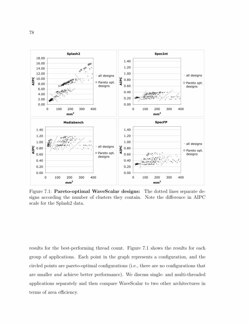
78
SpecInt
0.00
0.20
0.40
0.60
0.80
1.00
1.20
1.40
0 100 200 300 400
mm2
AIP
C
all designs
Pareto opt.designs
SpecFP
0.00
0.20
0.40
0.60
0.80
1.00
1.20
1.40
0 100 200 300 400
mm2
AIP
C
all designs
Pareto opt.designs
Mediabench
0.00
0.20
0.40
0.60
0.80
1.00
1.20
1.40
0 100 200 300 400
mm2
AIP
C all designs
Pareto opt.designs
Splash2
0.00
2.00
4.00
6.00
8.00
10.00
12.00
14.00
16.00
18.00
0 100 200 300 400
mm2
AIP
C
all designs
Pareto opt.designs
Figure 7.1: Pareto-optimal WaveScalar designs: The dotted lines separate de-signs according the number of clusters they contain. Note the di↵erence in AIPCscale for the Splash2 data.
results for the best-performing thread count. Figure 7.1 shows the results for each
group of applications. Each point in the graph represents a configuration, and the
circled points are pareto-optimal configurations (i.e., there are no configurations that
are smaller and achieve better performance). We discuss single- and multi-threaded
applications separately and then compare WaveScalar to two other architectures in
terms of area e�ciency.
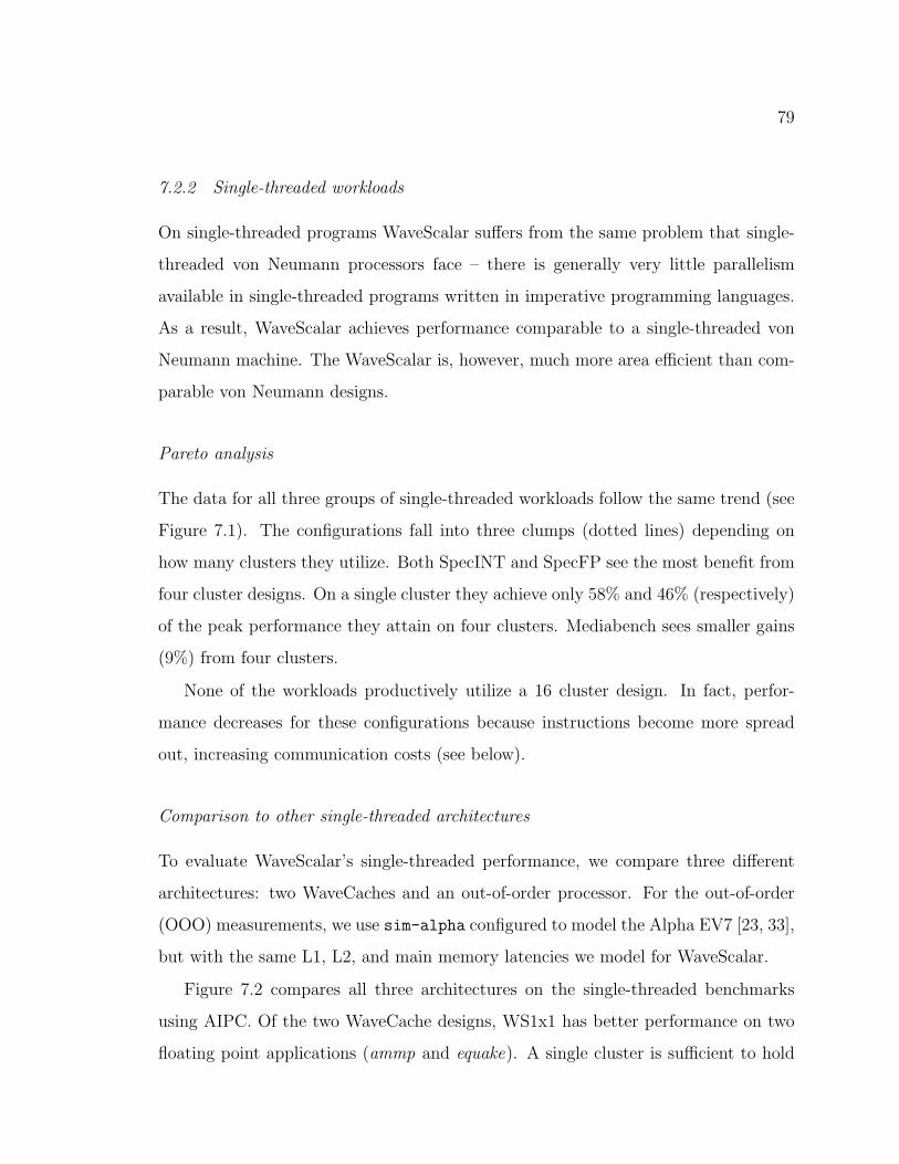
79
7.2.2 Single-threaded workloads
On single-threaded programs WaveScalar su↵ers from the same problem that single-
threaded von Neumann processors face – there is generally very little parallelism
available in single-threaded programs written in imperative programming languages.
As a result, WaveScalar achieves performance comparable to a single-threaded von
Neumann machine. The WaveScalar is, however, much more area e�cient than com-
parable von Neumann designs.
Pareto analysis
The data for all three groups of single-threaded workloads follow the same trend (see
Figure 7.1). The configurations fall into three clumps (dotted lines) depending on
how many clusters they utilize. Both SpecINT and SpecFP see the most benefit from
four cluster designs. On a single cluster they achieve only 58% and 46% (respectively)
of the peak performance they attain on four clusters. Mediabench sees smaller gains
(9%) from four clusters.
None of the workloads productively utilize a 16 cluster design. In fact, perfor-
mance decreases for these configurations because instructions become more spread
out, increasing communication costs (see below).
Comparison to other single-threaded architectures
To evaluate WaveScalar’s single-threaded performance, we compare three di↵erent
architectures: two WaveCaches and an out-of-order processor. For the out-of-order
(OOO) measurements, we use sim-alpha configured to model the Alpha EV7 [23, 33],
but with the same L1, L2, and main memory latencies we model for WaveScalar.
Figure 7.2 compares all three architectures on the single-threaded benchmarks
using AIPC. Of the two WaveCache designs, WS1x1 has better performance on two
floating point applications (ammp and equake). A single cluster is su�cient to hold
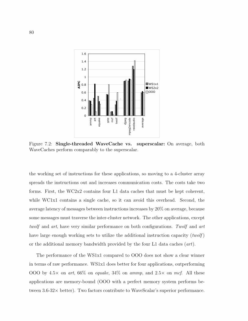
80
0
0.2
0.4
0.6
0.8
1
1.2
1.4
1.6
ammp
art
equake
gzip
mcf
twolf
djpeg
mpeg2encode
rawdaudio
average
AIPC
WS1x1
WS2x2
OOO
'
Figure 7.2: Single-threaded WaveCache vs. superscalar: On average, bothWaveCaches perform comparably to the superscalar.
the working set of instructions for these applications, so moving to a 4-cluster array
spreads the instructions out and increases communication costs. The costs take two
forms. First, the WC2x2 contains four L1 data caches that must be kept coherent,
while WC1x1 contains a single cache, so it can avoid this overhead. Second, the
average latency of messages between instructions increases by 20% on average, because
some messages must traverse the inter-cluster network. The other applications, except
twolf and art, have very similar performance on both configurations. Twolf and art
have large enough working sets to utilize the additional instruction capacity (twolf )
or the additional memory bandwidth provided by the four L1 data caches (art).
The performance of the WS1x1 compared to OOO does not show a clear winner
in terms of raw performance. WS1x1 does better for four applications, outperforming
OOO by 4.5⇥ on art, 66% on equake, 34% on ammp, and 2.5⇥ on mcf. All these
applications are memory-bound (OOO with a perfect memory system performs be-
tween 3.6-32⇥ better). Two factors contribute to WaveScalar’s superior performance.
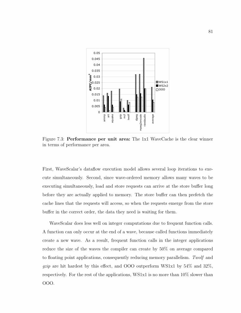
81
0
0.005
0.01
0.015
0.02
0.025
0.03
0.035
0.04
0.045
0.05
ammp
art
equake
gzip
mcf
twolf
djpeg
mpeg2encode
rawdaudio
average
AIPC/mm2
WS1x1
WS2x2
OOO
Figure 7.3: Performance per unit area: The 1x1 WaveCache is the clear winnerin terms of performance per area.
First, WaveScalar’s dataflow execution model allows several loop iterations to exe-
cute simultaneously. Second, since wave-ordered memory allows many waves to be
executing simultaneously, load and store requests can arrive at the store bu↵er long
before they are actually applied to memory. The store bu↵er can then prefetch the
cache lines that the requests will access, so when the requests emerge from the store
bu↵er in the correct order, the data they need is waiting for them.
WaveScalar does less well on integer computations due to frequent function calls.
A function can only occur at the end of a wave, because called functions immediately
create a new wave. As a result, frequent function calls in the integer applications
reduce the size of the waves the compiler can create by 50% on average compared
to floating point applications, consequently reducing memory parallelism. Twolf and
gzip are hit hardest by this e↵ect, and OOO outperform WS1x1 by 54% and 32%,
respectively. For the rest of the applications, WS1x1 is no more than 10% slower than
OOO.
82
The performance di↵erences between the two architectures are clearer if we take
into account the die area required for each processor. To estimate the size of OOO,
we examined a die photo of the EV7 in 180nm technology [33, 36]. The entire die is
396mm2. From this, we subtracted the area devoted to several components that our
RTL model does not include (e.g., the IO pads, and inter-chip network controller),
but would be present in a real WaveCache. We estimate the remaining area to be
⇠291mm2, with ⇠207mm2 devoted to 2MB of L2 cache. Scaling all these measure-
ments to 90nm technology yields ⇠72mm2 total and 51mm2 of L2. Measurements
from our RTL model show that WC1x1 occupies 48mm2 (12mm2 of L2 cache) and
WC2x2 occupies 247mm2 (48mm2 of L2 cache) in 90nm.
Figure 7.3 shows the area-e�ciency of the WaveCaches measured in AIPC/mm2
compared to OOO. For our single threaded workloads, OOO achieves an area e�ciency
of 0.008 AIPC/mm2 and a bottom-line performance of 0.6 AIPC. Depending on the
configuration, WaveScalar’s e�ciency for the single-threaded applications is between
0.004 AIPC/mm2 (0.71 AIPC; configuration 31) and 0.033 AIPC/mm2 (0.45 AIPC;
configuration 1). WaveScalar configuration 4 closely matches the OOO’s performance,
but is 50% more area-e�cient.
In summary, for most of our workloads, the WaveCache’s bottom-line single-
threaded AIPC is as good as or better than conventional superscalar designs, and
it achieves this level of performance with a less complicated design and in a smaller
area.
7.2.3 Multi-threaded workloads
The multi-threaded Splash2 benchmarks provide ample parallelism and can take ad-
vantage of much larger WaveScalar designs. They also a↵ord an opportunity to com-
pare WaveScalar’s multithreading abilities to those of CMPs.
83
Pareto analysis
Figure 7.1 (upper left) shows WaveScalar’s performance for multithreaded workloads.
Because the workloads are multithreaded, they can take advantage of additional area
very e↵ectively, as both performance and area increase at nearly the same rate. The
dotted lines divide the designs into groups of 1-, 4-, and 16-cluster configurations. The
wide, horizontal gap at ⇠6 IPC is a result of running di↵erent numbers of threads.
For each configuration, we run a range of di↵erent thread counts for each application
and report the best overall performance. Designs above the gap generally have larger
virtualization degrees (i.e., the number of instructions that can reside at a PE) and L1
data caches, allowing them to support more threads simultaneously providing more
parallelism.
Table 7.4 lists the pareto-optimal configurations for Splash2 divided into five
groups of designs with similar performance (column “Avg. AIPC”).
Group A is the single-cluster configurations. Designs 1, 2, 5, and 6 contain only
two domains per cluster. Designs 5 and 6 outperform smaller, four-domain designs
(3 and 4) because pressure in the L1 data cache outweighs the benefits of additional
processing elements.
Moving to four clusters without an L2 cache (Group B) increases the chip’s size by
52% and its performance by 38%. Doubling the size of the L1 provides an additional
11% performance boost.
Group C (configurations 13 and 14) “trades-in” large L1 caches for an on-chip
L2. For configuration 13, this results in a 43.5% improvement in performance for a
negligible increase in area.
The first four 4-cluster designs (Groups B and C) all have much smaller virtu-
alization degrees than the best-performing single-cluster designs (64 vs. 128-256).
Configuration 15, the first in Group D, has 128 instructions per PE. The change leads
to 43% more performance and requires only 12% additional area.
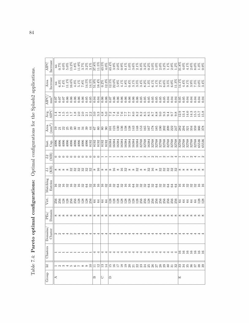
84Tab
le7.
4:Pare
toopti
malco
nfigura
tions:
Optim
alco
nfigu
rati
ons
for
the
Spla
sh2
applica
tion
s.
Group
Id
Clusters
Dom
ains/
PE
s/
Virt.
Matching
L1
L2
Inst.
Area
Avg.
AIP
C/
Area
AIP
C
Cluster
Dom
ain
Entries
(K
B)
(M
B)
Cap.
(m
m
2)
AIP
Cm
m
2Increase
Increase
A1
12
8256
16
80
4096
19
1.4
0.07
na
na
21
28
256
32
80
4096
21
1.4
0.07
6.3%
0.7%
31
48
128
16
80
4096
22
1.5
0.07
7.4%
4.0%
41
48
128
32
80
4096
25
1.5
0.06
11.1%
5.0%
51
28
256
16
32
04096
29
1.7
0.06
16.6%
13.2%
61
28
256
32
32
04096
30
1.8
0.06
4.3%
1.8%
71
48
128
16
32
04096
31
2.0
0.06
5.1%
11.9%
81
48
128
32
32
04096
34
2.0
0.06
7.8%
3.7%
91
48
128
64
32
04096
39
2.1
0.05
14.5%
3.2%
10
14
8256
32
32
08192
44
2.2
0.05
14.5%
3.1%
B11
44
864
16
80
8192
67
3.0
0.04
51.9%
37.8%
12
44
864
16
16
08192
80
3.3
0.04
18.4%
11.5%
C13
44
864
16
81
8192
80
4.8
0.06
0.2%
43.5%
14
44
864
32
81
8192
90
5.0
0.06
12.3%
4.0%
D15
44
8128
16
81
16384
101
7.2
0.07
12.5%
43.4%
16
44
8128
32
16
116384
123
7.4
0.06
22.0%
3.9%
17
44
8128
64
81
16384
130
7.6
0.06
5.9%
2.0%
18
44
8128
32
16
216384
136
7.6
0.06
4.1%
0.9%
19
44
8128
16
32
116384
138
7.7
0.06
1.8%
0.1%
20
44
8128
16
84
16384
138
7.7
0.06
0.4%
1.0%
21
44
8128
64
82
16384
143
8.0
0.06
3.1%
3.6%
22
44
8128
32
32
116384
148
8.2
0.06
3.5%
2.1%
23
44
8256
32
81
32768
153
8.2
0.05
3.4%
0.3%
24
44
8256
32
82
32768
165
8.5
0.05
8.2%
3.2%
25
44
8128
64
32
116384
167
8.5
0.05
1.3%
0.2%
26
44
8256
32
16
232768
178
8.7
0.05
6.1%
3.0%
27
44
8256
64
82
32768
185
8.8
0.05
4.1%
1.0%
28
44
8256
32
32
132768
190
9.0
0.05
2.7%
2.0%
29
44
8256
32
32
232768
202
9.3
0.05
6.6%
3.2%
30
44
8256
64
32
132768
209
9.4
0.04
3.5%
1.1%
31
44
8256
64
32
232768
222
9.7
0.04
6.0%
2.9%
32
44
8256
64
32
432768
247
9.8
0.04
11.3%
1.2%
E33
16
48
64
16
81
32768
282
12.9
0.05
14.1%
31.8%
34
16
48
64
16
82
32768
294
13.4
0.05
4.4%
4.0%
35
16
48
64
32
81
32768
321
14.0
0.04
9.1%
4.1%
36
16
48
64
32
82
32768
334
14.3
0.04
3.9%
2.6%
37
16
48
64
32
84
32768
359
15.5
0.04
7.5%
8.0%
38
16
48
128
16
81
65536
366
15.7
0.04
2.0%
1.3%
39
16
48
128
16
82
65536
378
15.8
0.04
3.4%
0.9%
85
The remaining designs in Group D increase slowly in area and performance. Vir-
tualization degree is most important to performance followed by matching table size
and cache capacity. With few exceptions, the gains in performance are smaller than
the increase in area that they require. As a result, the area e�ciency of the designs
falls from 0.07 AIPC/mm2 to 0.04 AIPC/mm2.
The designs in Group D are the best example of a phenomenon that also occurs in
Group A and among the largest pareto-optimal designs for SpecINT and mediabench.
In each case, increases in area lead to small changes in performance. This suggests
that within those size ranges (19-44mm2 for Group A and 101-247mm2 for Group
D) the designs are as balanced as possible without moving to significantly larger
configurations. However, Groups A and D end when the number of PEs increases,
demonstrating that the availability of PEs is the key constraint on performance of
the smaller designs. For the largest SpecINT and mediabench designs, the data tell
a di↵erent story. In those cases, the limiting factor is parallelism in the application,
and no amount of additional hardware can improve performance.
The configurations in Group E (33-39) have 16 clusters. The transition from 4 to
16 clusters mimics the transition from 1 to 4: The smallest 16 cluster designs have less
virtualization and increase their performance by increasing matching table capacity
and cache sizes. The larger designs “trade-in” matching table capacity for increased
virtualization.
The results demonstrate that WaveScalar is scalable both in terms of area e�-
ciency and peak performance. Design 3 is the most area e�cient design, and de-
sign 15 uses the same cluster configuration to achieve the same level of e�ciency
(0.07 AIPC/mm2). As a result, the designs are approximately a factor of 5 apart in
both area and performance. Scaling the same cluster configuration to a 16-cluster
machine (configuration 38) reduces the area e�ciency to 0.04 AIPC/mm2, however.
A more area-e�cient alternative (0.05 AIPC/mm2) is configuration 33, which corre-
sponds to scaling up configuration 13 and using a slightly smaller L2 data cache.
86
Design 10 outperforms all the other 1 cluster designs (2.2 AIPC), and configuration
28 uses the same cluster design to achieve 4.2⇥ the performance (9 AIPC) in 4.6⇥ the
area. This level of performance is within 5% of the best performing 4-cluster design
(configuration 32), demonstrating scalability of raw performance.
This slightly imperfect scalability (the last 5%), however, raises complex questions
for chip designers. For instance, if an implementation of configuration 38’s cluster
is available (e.g., from an implementation of configuration 3), is it more economic
to quickly build that larger, slightly less e�cient design or to expend the design
and verification e↵ort to implement configuration 33 instead? At the very least, it
suggests tiled architectures are not perfectly scalable, but rather scalability claims
must be carefully analyzed.
Larger designs
To evaluate the WaveCache’s multithreaded performance more thoroughly, we simu-
late a 64-cluster design, representing an aggressive “big iron” processor built in next-
generation process technology and evaluated its performance using Splash2. Then, to
place the multithreaded results in context with contemporary designs, we compare a
smaller, 16-cluster array that could be built today with a range of multithreaded von
Neumann processors from the literature. For the workloads the studies have in com-
mon, the 16-cluster WaveCache outperforms the von Neumann designs by a factor of
between 2 and 16.
We simulate an 8x8 array of clusters (based on configuration 14 in Table 7.4) to
model an aggressive, future-generation design. Using the results from our area model
scaled to 45nm, we estimate that the processor occupies ⇠360mm2, with an on-chip
16MB L2.
Our performance metric is execution-time speedup relative to a single thread exe-
cuting on the same WaveCache. We also compare the WaveScalar speedups to those
calculated by other researchers for other threaded architectures. Component metrics
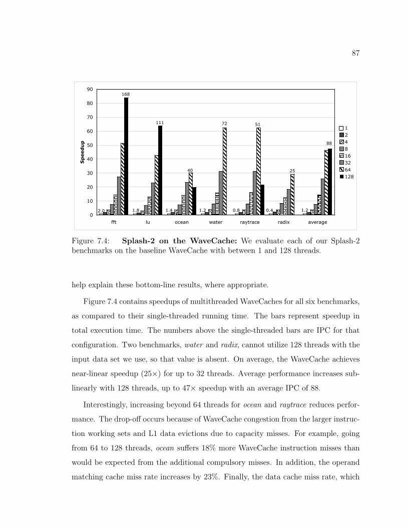
87
0
10
20
30
40
50
60
70
80
90
fft lu ocean water raytrace radix average
Speedup
1
2
4
8
16
32
64
128
2.0
168
1.8
111
1.4
40
1.2
72
0.8
51
0.4
25
1.2
88
Figure 7.4: Splash-2 on the WaveCache: We evaluate each of our Splash-2benchmarks on the baseline WaveCache with between 1 and 128 threads.
help explain these bottom-line results, where appropriate.
Figure 7.4 contains speedups of multithreaded WaveCaches for all six benchmarks,
as compared to their single-threaded running time. The bars represent speedup in
total execution time. The numbers above the single-threaded bars are IPC for that
configuration. Two benchmarks, water and radix, cannot utilize 128 threads with the
input data set we use, so that value is absent. On average, the WaveCache achieves
near-linear speedup (25⇥) for up to 32 threads. Average performance increases sub-
linearly with 128 threads, up to 47⇥ speedup with an average IPC of 88.
Interestingly, increasing beyond 64 threads for ocean and raytrace reduces perfor-
mance. The drop-o↵ occurs because of WaveCache congestion from the larger instruc-
tion working sets and L1 data evictions due to capacity misses. For example, going
from 64 to 128 threads, ocean su↵ers 18% more WaveCache instruction misses than
would be expected from the additional compulsory misses. In addition, the operand
matching cache miss rate increases by 23%. Finally, the data cache miss rate, which
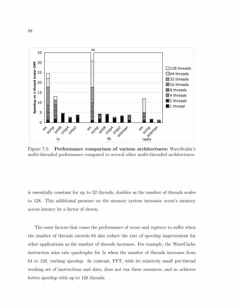
88
0
5
10
15
20
25
30
35
ws
scmp
smt8
cmp4
cmp2 w
s
scmp
smt8
cmp4
cmp2
eckm
an ws
scmp
eckm
an
Sp
eed
up
vs 1
-th
read
scala
r C
MP
128 threads
64 threads
32 threads
16 threads
8 threads
4 threads
2 threads
1 thread
46
lu fft radix
Figure 7.5: Performance comparison of various architectures: WaveScalar’smulti-threaded performance compared to several other multi-threaded architectures.
is essentially constant for up to 32 threads, doubles as the number of threads scales
to 128. This additional pressure on the memory system increases ocean’s memory
access latency by a factor of eleven.
The same factors that cause the performance of ocean and raytrace to su↵er when
the number of threads exceeds 64 also reduce the rate of speedup improvement for
other applications as the number of threads increases. For example, the WaveCache
instruction miss rate quadruples for lu when the number of threads increases from
64 to 128, curbing speedup. In contrast, FFT, with its relatively small per-thread
working set of instructions and data, does not tax these resources, and so achieves
better speedup with up to 128 threads.

89
Comparison to other multi-threaded architectures
To understand how WaveCache performance compares with other architectures we
perform two sets of experiments. In the first, we compare WaveCache performance to
other multi-threaded architectures on three Splash-2 kernels: lu, ↵t and radix. Then
we compare its area e�ciency to the Niagara processor from Sun.
To compare our Splash2 performance to other threaded processors, we present
results from several sources in addition to our own WaveCache simulator. For CMP
configurations we performed our own experiments using a simple in-order core (scmp),
as well as measurements from [40] and [24]. Comparing data from such diverse sources
is di�cult, and drawing precise conclusions about the results is not possible. However,
we believe that the measurements are valuable for the broad trends they reveal.
To make the comparison as equitable as possible, we use a smaller, 4x4 WaveCache
for these studies. Our RTL model gives an area of 253mm2 for this design (we assume
an o↵-chip, 16 MB L2 cache and increase its access time from 10 to 20 cycles).
While we do not have precise area measurements for the other architectures, the
most aggressive configurations (i.e., most cores or functional units) are in the same
ball park with respect to size.
To facilitate the comparison of performance numbers of these di↵erent sources,
we normalized all performance numbers to the performance of a simulated scalar
processor with a 5-stage pipeline. The processor has 16KB data and instruction
caches, and a 1MB L2 cache, all 4-way set associative. The L2 hit latency is 12
cycles, and the memory access latency of 200 cycles matches that of the WaveCache.
Figure 7.5 shows the results. The stacked bars represent the increase in perfor-
mance contributed by executing with more threads. The bars labeled ws depict the
performance of the WaveCache. The bars labeled scmp represent the performance of
a CMP whose cores are the scalar processors described above with 1MB of L2 cache
per processor core. These processors are connected via a shared bus between pri-

90
vate L1 caches and a shared L2 cache. Memory is sequentially consistent and uses a
snooping version of the protocol WaveScalar’s L1 data caches use. Up to 4 accesses to
the shared memory may overlap. For the CMPs the stacked bars represent increased
performance from simulating more processor cores. The 4- and 8-core bars loosely
model Hydra [31] and a single Piranha chip [10], respectively.
The bars labeled smt8, cmp4 and cmp2 are the 8-threaded SMT and 4- and 2-core
out-of-order CMPs from [40]. We extracted their running times from data provided
by the authors. Memory latency is low on these systems (dozens of cycles) compared
to expected future latencies, and all configurations share the L1 data- and instruction
caches.
To compare the results from [24] (labeled ekman in the figure), which are nor-
malized to the performance of their 2-core CMP, we simulated a superscalar with a
configuration similar to one of these cores and halved the reported execution time;
we then used this figure as an estimate of absolute baseline performance. In [24],
the authors fixed the execution resources for all configurations, and partitioned them
among an increasing number of decreasingly wide CMP cores. For example, the 2-
thread component of the ekman bars is the performance of a 2-core CMP in which
each core has a fetch width of 8, while the 16-thread component represents the per-
formance of 16 cores with a fetch-width of 1. Latency to main memory is 384 cycles,
and latency to the L2 cache is 12 cycles.
The data show that the WaveCache can handily outperform the other architec-
tures at high thread counts. It executes 1.8⇥ to 10.9⇥ faster than scmp, 5.2⇥ to
10.8⇥ faster than smt8, and 6.4⇥ to 16.6⇥ faster than the various out-of-order CMP
configurations. Component metrics show that the WaveCache’s performance benefits
arise from its use of point-to-point communication, rather than a system-wide broad-
cast mechanism, and from the latency-tolerance of its dataflow execution model. The
former enables scaling to large numbers of clusters and threads, while the latter helps
mask the increased memory latency incurred by the directory protocol and the high
91
load-use penalty on the L1 data cache.
The performance of all systems eventually plateaus when some bottleneck resource
saturates. For scmp this resource is shared L2 bus bandwidth. Bus saturation occurs
at 16 processors for LU, 8 for FFT and 2 for RADIX1. For the other von Neumann
CMP systems, the fixed allocation of execution resources is the limit [40], resulting
in a decrease in per-processor IPC. For example, in ekman, per-processor IPC drops
50% as the number of processors increases from 4 to 16 for RADIX and FFT. On
the WaveCache, speedup plateaus when the working set of all the threads equals its
instruction capacity. This o↵ers the WaveCache the opportunity to tune the number of
threads to the amount of on-chip resources. With their static partitioning of execution
resources across processors, this option is absent for CMPs; and the monolithic nature
of SMT architectures prevents scaling to large numbers of thread contexts.
Finally, we compare the WaveCache to Sun’s Niagara processor [37] in terms of
area e�ciency. Niagara is an 8-way CMP targeted at large multi-threaded workloads.
We are unaware of any published evaluation of Splash2 on Niagara, but [37] shows
Niagara running at 4.4 IPC (0.55 IPC/core) at 1.2 GHz (an approximately 10%
faster clock than WaveScalar’s). Niagara’s die measures 379mm2, giving an e�ciency
of 0.01 IPC/mm2. Since each Niagara core is single-issue and in-order, and all eight
cores share a floating point unit, the theoretical maximum e�ciency is 0.02 IPC/mm2.
The least e�cient pareto optimal WaveScalar design (configuration 39) is twice as
e�cient (0.04 AIPC/mm2).
Discussion
The WaveCache has clear promise as a multiprocessing platform. In the 90nm technol-
ogy available today, we could easily build a WaveCache that would outperform a range
1While a 128-core scmp with a more sophisticated coherence system might perform more com-petitively with the WaveCache on RADIX and FFT, studies of these systems are not present inthe literature, and it is not clear what their optimal memory system design would be.
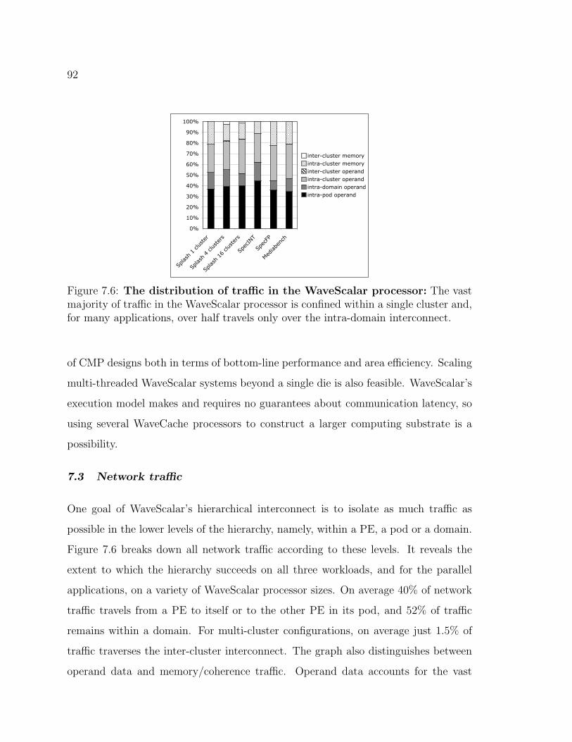
92
0%
10%
20%
30%
40%
50%
60%
70%
80%
90%
100%
Splas
h 1 clus
ter
Splas
h 4 clus
ters
Splas
h 16
cluster
s
Spe
cINT
Spe
cFP
Med
iabe
nch
inter-cluster memory
intra-cluster memory
inter-cluster operand
intra-cluster operand
intra-domain operand
intra-pod operand
Figure 7.6: The distribution of tra�c in the WaveScalar processor: The vastmajority of tra�c in the WaveScalar processor is confined within a single cluster and,for many applications, over half travels only over the intra-domain interconnect.
of CMP designs both in terms of bottom-line performance and area e�ciency. Scaling
multi-threaded WaveScalar systems beyond a single die is also feasible. WaveScalar’s
execution model makes and requires no guarantees about communication latency, so
using several WaveCache processors to construct a larger computing substrate is a
possibility.
7.3 Network tra�c
One goal of WaveScalar’s hierarchical interconnect is to isolate as much tra�c as
possible in the lower levels of the hierarchy, namely, within a PE, a pod or a domain.
Figure 7.6 breaks down all network tra�c according to these levels. It reveals the
extent to which the hierarchy succeeds on all three workloads, and for the parallel
applications, on a variety of WaveScalar processor sizes. On average 40% of network
tra�c travels from a PE to itself or to the other PE in its pod, and 52% of tra�c
remains within a domain. For multi-cluster configurations, on average just 1.5% of
tra�c traverses the inter-cluster interconnect. The graph also distinguishes between
operand data and memory/coherence tra�c. Operand data accounts for the vast

93
majority of messages, 80% on average, with memory tra�c less than 20%.
These results demonstrate the scalability of communication performance on the
WaveScalar processor. Applications that require only a small patch of the processor,
such as Spec2000, can execute without ever paying the price for long distance commu-
nication. In addition, the distribution of tra�c types barely changes with the number
of clusters, indicating that the interconnect partitioning scheme is scalable. Message
latency does increase with the number of clusters (by 12% from 1 to 16 clusters), but
as we mentioned above, overall performance still scales linearly. One reason for the
scalability is that the WaveScalar instruction placement algorithms isolate individual
Splash threads into di↵erent portions of the die. Consequently, although the average
distance between two clusters in the processor increases from 0 (since there is only
one cluster) to 2.8, the average distance that a message travels increases by only 6%.
For the same reason, network congestion increases by only 4%.
7.4 Discussion
We have presented a design space analysis for WaveScalar processors implemented in
an ASIC tool flow. However, our conclusions also apply to full-custom WaveScalar
designs and, in some ways, to other tiled architectures such as CMPs.
The two main conclusions would not change in a full-custom design. For the first
conclusion, that WaveScalar is inherently scalable both in terms of area e�ciency
and raw performance, our data provide a lower bound on WaveScalar’s ability to
scale. Custom implementations should lead to smaller designs, faster designs, or
both. Our second conclusion, that WaveScalar’s area e�ciency compares favorably
to more conventional designs, would hold in a full custom design for the same reason.
WaveScalar’s hierarchical interconnect would serve well as the interconnect for an
aggressive CMP design, and our results concerning the scalability and performance of
the network would apply to that domain as well. In a conventional CMP design, the
network carries coherence tra�c, but as researchers strive to make CMPs easier to
94
program it might make sense to support other types of data, such as MPI messages,
as well. In that case, our data demonstrate the value of localizing communication
as much as possible and the feasibility of using a single network for both coherence
tra�c and data messaging.
95
Chapter 8
WAVESCALAR’S DATAFLOW FEATURES
The WaveScalar instruction set and hardware design we have described so far
replicates the functionality of a von Neumann processor or a CMP composed of von
Neumann processors. Providing these capabilities is essential for WaveScalar to be
a viable alternative to von Neumann architectures, but it is not the limit of what
WaveScalar can do.
This chapter exploits WaveScalar’s dataflow underpinning to achieve two things
that conventional von Neumann machines cannot. First, it provides a second, un-
ordered memory interface that is similar to the token-passing interface in Section 3.4.1.
The unordered interface is built to express memory parallelism. It bypasses the wave-
ordered store bu↵er and accesses the L1 cache directly, avoiding the overhead of the
wave-ordering hardware. Because the unordered operations do not go through the
store bu↵er, they can arrive at the L1 cache in any order or in parallel.
Second, the WaveCache can support very fine-grain threads. On von Neumann
machines the amount of hardware devoted to a thread is fixed (e.g., one core on a
CMP or one thread context on an SMT machine), and the number of threads that can
execute at once is relatively small. On the WaveCache, the number of physical store
bu↵ers limits the number of threads that use wave-ordered memory simultaneously,
but any number of threads can use the unordered interface at one time. In addition,
spawning these threads is even less expensive than spawning threads that use the
wave-ordered interface (Section 5.1), so it is feasible to break a program up into 100s
of parallel, fine-grain threads.
We begin by describing the unordered memory interface. Then we use it and
96
fine-grain threads to express large amounts of parallelism in three application ker-
nels. Finally, we combine the two styles of programming to parallelize equake from
the Spec2000 floating point suite, and demonstrate that by combining WaveScalar’s
ability to run both kinds (i.e., coarse-grain, von Neumann-style threads and fine-
grain, dataflow-style threads), we can achieve performance greater than utilizing ei-
ther alone, in this case, a 9⇥ speedup.
8.1 Unordered memory
As described, WaveScalar’s only mechanism for accessing memory is the wave-ordered
memory interface. The interface is necessary for executing conventional programs, but
it can only express limited parallelism (i.e., by using ripple numbers). WaveScalar’s
unordered interface makes a di↵erent trade-o↵: it cannot e�ciently provide the se-
quential ordering that conventional programs require, but it excels at expressing par-
allelism, because it eliminates unneeded ordering constraints and avoids contention
for the store bu↵er. Because of this, it allows programmers or compilers to express
and exploit memory parallelism when they know it exists.
Like all other dataflow instructions, unordered operations are only constrained by
their static data dependences. This means that if two unordered memory operations
are not directly or indirectly data-dependent, they can execute in any order. Pro-
grammers and compilers can exploit this fact to express parallelism between memory
operations that can safely execute out of order; however, they need a mechanism to
enforce ordering among those that cannot.
To illustrate, consider a Store and a Load that could potentially access the
same address. If, for correct execution, the Load must see the value written by the
Store (i.e., a read-after-write dependence), then the thread must ensure that the
Load does not execute until the Store has finished. If the thread uses wave-ordered
memory, the store bu↵er enforces this constraint; however, since unordered memory
operations bypass the wave-ordered interface, unordered accesses must use a di↵erent

97
mechanism.
To ensure that the Load executes after the Store, there must be a data depen-
dence between them. This means memory operations must produce an output token
that can be passed to the operations that follow. Loads already do this, because
they return a value from memory. We modify Stores to produce a value when they
complete. The value that the token carries is unimportant, since its only purpose is to
signal that the Store is complete. In our implementation it is always zero. We call
unordered Loads and Stores, Load-Unordered and Store-Unordered-Ack,
respectively.
8.1.1 Performance evaluation
To demonstrate the potential of unordered memory, we implemented three tradi-
tionally parallel but memory-intensive kernels – matrix multiply (MMUL), longest
common subsequence (LCS), and a finite input response filter (FIR) – in three di↵er-
ent styles and compared their performance. Serial coarse-grain uses a single thread
written in C. Parallel coarse-grain is a coarse-grain parallelized version, also written
in C, that uses the coarse-grain threading mechanisms described in Chapter 5. Un-
ordered uses a single coarse-grain thread written in C to control a pool of fine-grain
threads that use unordered memory, written in WaveScalar assembly. We call these
unordered threads.
For each application, we tuned the number of threads and the array tile size
to achieve the best performance possible for a particular implementation. MMUL
multiplies 128 ⇥ 128 entry matrices, LCS compares strings of 1024 characters, and
FIR filters 8192 inputs with 256 taps. They use between 32 (FIR) and 1000 (LCS )
threads. Each version is run to completion.
Figure 8.1 depicts the performance of each algorithm executing on the 8x8 Wave-
Cache described in Section 7.2.3. On the left, it shows speedup over the serial imple-
mentation, and, on the right, average units of work completed per cycle. For MMUL

98
0
50
100
150
200
250
300
mmul lcs fir
Sp
eed
up
vs s
ing
le-t
hread
ed
`
0
2
4
6
8
10
12
14
16
mmul lcs fir
Ap
plicati
on
wo
rk u
nit
s p
er c
ycle
`
single-threadedfine-grain
coarse-grain
Figure 8.1: Fine-grain performance: Performance of three di↵erent implementa-tion styles
and FIR, the unit of work selected is a multiply-accumulate, while for LCS, it is a
character comparison. We use application-specific performance metrics, because they
are more informative than IPC when comparing the three implementations. For all
three kernels, the unordered implementations achieve superior performance because
they exploit more parallelism.
The benefits stem from two sources. First, the unordered implementations can use
more threads. It would be easy to write a pthread-based version that spawned 100s
or 1000s of threads, but the WaveCache cannot execute that many ordered threads
at once, since there are not enough store bu↵ers. Secondly, the unordered threads’
memory operations can execute in parallel. As a result, the fine-grain, unordered
implementation exploit more inter- and intra-thread parallelism. MMUL is the best
example; it executes 27 memory operations per cycle on average (about one per every
two clusters), compared to just 6 for the coarse-grain version.
FIR and LCS are less memory-bound than MMUL because they load values (input
samples for FIR and characters for LCS ) from memory once and then pass them from
thread to thread directly. For these two applications the limiting factor is inter-cluster
99
network bandwidth. Both algorithms involve a great deal of inter-thread communi-
cation, and since the computation uses the entire 8x8 array of clusters, inter-cluster
communication is unavoidable. For LCS 27% of messages travel across the inter-
cluster network compared to 0.4-1% for the single-threaded and coarse-grain versions,
and the messages move 3.6 times more slowly due to congestion. FIR displays similar
behavior. A di↵erent placement algorithm might alleviate much of this problem and
improve performance further by placing the instructions for communicating threads
near one another.
8.2 Mixing threading models
In Chapter 5, we explained the extensions to WaveScalar that support coarse-grain,
pthread-style threads. In the previous section, we introduced two lightweight memory
instructions that enable fine-grain threads and unordered memory. In this section,
we combine these two models; the result is a hybrid programming model that enables
coarse- and fine-grain threads to coexist in the same application. We begin with two
examples that illustrate how ordered and unordered memory operations can be used
together. Then, we exploit all of our threading techniques to improve the performance
of Spec2000’s equake by a factor of nine.
8.2.1 Mixing ordered and unordered memory
A key strength of our ordered and unordered memory mechanisms is their ability
to coexist in the same application. Sections of an application that have independent
and easily analyzable memory access patterns (e.g., matrix manipulations and stream
processing) can use the unordered interface, while di�cult to analyze portions (e.g.,
pointer-chasing codes) can use wave-ordered memory.
We describe two ways to combine ordered and unordered memory accesses. The
first turns o↵ wave-ordered memory, uses the unordered interface, and then reinstates
wave-ordering. The second, more flexible approach allows the ordered and unordered

100
ThreadToData
MemorySequenceStop
<t:w>.finished
<t:w>.v
<t:w>.t
MemorySequenceStart
<t:w>.w
WaveToData<t:w>.t
Arbitrary unordered code
Ordered Code
Ordered Code
Figure 8.2: Transitioning between memory interfaces: The transition from or-dered to unordered memory and back again.
interfaces to exist simultaneously.
Example 1 Figure 8.2 shows a code sequence that transitions from wave-ordered
memory to unordered memory and back again. The process is quite similar to ter-
minating and restarting a pthread-style thread. At the end of the ordered code, a
Thread-To-Data instruction extracts the current Thread-Id, and a Memory-
Sequence-Stop instruction terminates the current memory ordering. Memory-
Sequence-Stop outputs a value, labeled finished in the figure, after all preceding
wave-ordered memory operations have completed. The finished token triggers the
dependent, unordered memory operations, ensuring that they do not execute until
the earlier, ordered-memory accesses have completed.
After the unordered portion has executed, a Memory-Sequence-Start creates
a new, ordered memory sequence using the Thread-Id extracted previously. In
principle, the new thread need not have the same Thread-Id as the original ordered
thread. In practice, however, this is convenient, as it allows values to flow directly
from the first ordered section to the second (the curved arcs on the left side of the
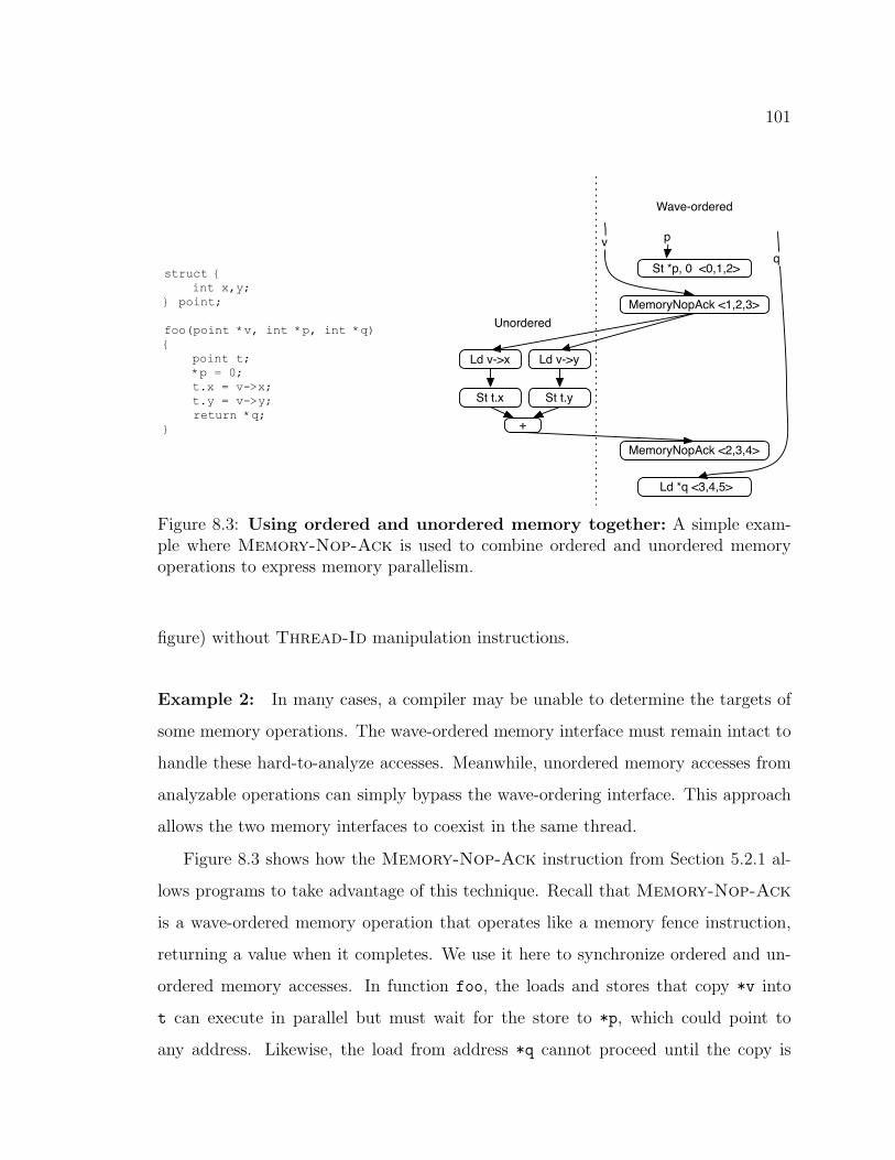
101
struct {
int x,y;
} point;
foo(point *v, int *p, int *q)
{
point t;
*p = 0;
t.x = v->x;
t.y = v->y;
return *q;
}
St *p, 0 <0,1,2>
MemoryNopAck <1,2,3>
Ld v->x Ld v->y
St t.x St t.y
MemoryNopAck <2,3,4>
+
pv
Wave-ordered
Unordered
Ld *q <3,4,5>
q
Figure 8.3: Using ordered and unordered memory together: A simple exam-ple where Memory-Nop-Ack is used to combine ordered and unordered memoryoperations to express memory parallelism.
figure) without Thread-Id manipulation instructions.
Example 2: In many cases, a compiler may be unable to determine the targets of
some memory operations. The wave-ordered memory interface must remain intact to
handle these hard-to-analyze accesses. Meanwhile, unordered memory accesses from
analyzable operations can simply bypass the wave-ordering interface. This approach
allows the two memory interfaces to coexist in the same thread.
Figure 8.3 shows how the Memory-Nop-Ack instruction from Section 5.2.1 al-
lows programs to take advantage of this technique. Recall that Memory-Nop-Ack
is a wave-ordered memory operation that operates like a memory fence instruction,
returning a value when it completes. We use it here to synchronize ordered and un-
ordered memory accesses. In function foo, the loads and stores that copy *v into
t can execute in parallel but must wait for the store to *p, which could point to
any address. Likewise, the load from address *q cannot proceed until the copy is
102
complete. The wave-ordered memory system guarantees that the store to *p, the two
Memory-Nop-Acks, and the load from *q fire in the order shown (top to bottom).
The data dependences between the first Memory-Nop-Ack and the unordered loads
at left ensure that the copy occurs after the first store. The Add instruction sim-
ply coalesces the outputs from the two Store-Unordered-Ack instructions into a
trigger for the second Memory-Nop-Ack that ensures the copy is complete before
the final load.
8.2.2 A detailed example: equake
To demonstrate that mixing the two threading styles is not only possible but also
profitable, we optimized equake from the SPEC2000 benchmark suite. equake spends
most of its time in the function smvp, with the bulk of the remainder confined to a
single loop in the program’s main function. In the discussion below, we refer to this
loop in main as sim.
We exploit both ordered, coarse-grain and unordered, fine-grain threads in equake.
The key loops in sim are data independent, so we parallelized them using coarse-grain
threads that process a work queue of blocks of iterations. This optimization improves
sim’s performance by 2.2⇥, but speeds up equake by only a factor of 1.6 overall.
Next, we used the unordered memory interface to exploit fine-grain parallelism in
smvp. Two opportunities present themselves. First, each iteration of smvp’s nested
loops loads data from several arrays. Since these arrays are read-only, we used un-
ordered loads to bypass wave-ordered memory, allowing loads from several iterations
to execute in parallel. Second, we targeted a set of irregular cross-iteration depen-
dences in smvp’s inner loop that are caused by updating an array of sums. These
cross-iteration dependences make it di�cult to profitably coarse-grain-parallelize the
loop. However, the Thread-Coordinate instruction lets us extract fine-grain par-
allelism despite these dependences, since it e�ciently passes array elements from PE
to PE and guarantees that only one thread can hold a particular value at a time. This
103
idiom is inspired by M-structures [11], a dataflow-style memory element. Rewriting
smvp with unordered memory and Thread-Coordinate improves that functions
performance by 11⇥, but overall gains are only 2.2⇥.
When both coarse-grain and fine-grain threading are used together, equake speeds
up by a factor of 9.0. This result demonstrates that coarse-grain, pthread-style threads
and fine-grain, unordered threads can be combined to accelerate a single application
beyond what either technique can achieve in isolation.
104
Chapter 9
RELATED WORK
WaveScalar is the most recent in a long line of dataflow processor architectures,
but its goal di↵ers in some ways from its predecessors. Previous dataflow machines
focused (mostly) on performance for scientific computing, and the key advantage of
dataflow was the parallelism it could express and exploit. WaveScalar’s approach
di↵ers in two respects. First, it targets general purpose programs and imperative
programming languages. Second, although it takes advantage of dataflow parallelism,
it exploits dataflow’s decentralized execution model to address the challenges that
face modern chip designers.
In this regard, WaveScalar resembles other tiled architectures that researchers
have proposed. These designs strive to reduce design e↵ort by replicating hardware
structures across the silicon die. The dataflow execution model is a natural match for
such a design.
This chapter places WaveScalar in context relative to both previous dataflow de-
signs and modern tiled architectures. It also addresses several arguments against the
dataflow model as the basis for scalable processor designs.
9.1 Previous dataflow designs
Dataflow execution models, by definition, share two characteristics. First, they rep-
resent programs as dataflow graphs. The nodes in the graph are operations and the
dataflow arcs between them carry data values from one operation to another. Sec-
ond, execution occurs according to the dataflow firing rule. That is, an operation may
execute when its inputs are available.
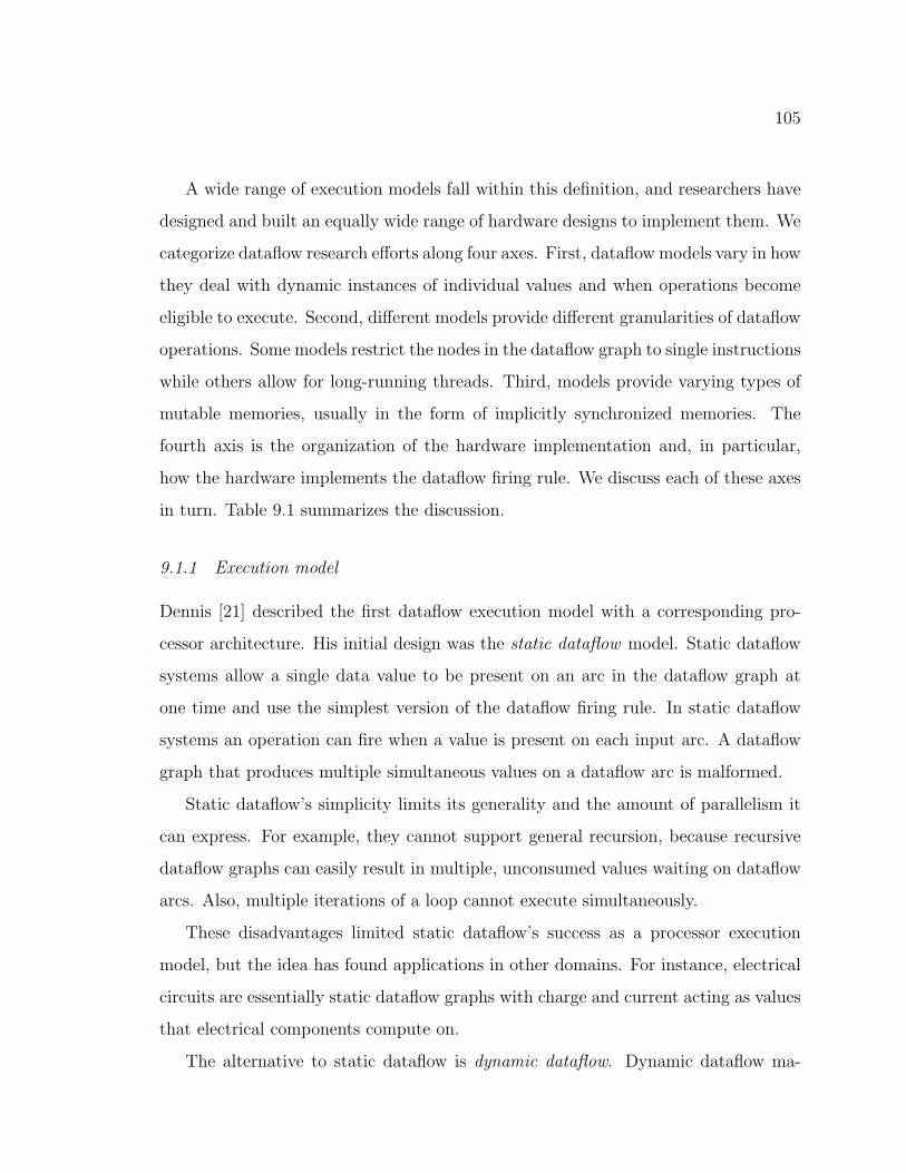
105
A wide range of execution models fall within this definition, and researchers have
designed and built an equally wide range of hardware designs to implement them. We
categorize dataflow research e↵orts along four axes. First, dataflow models vary in how
they deal with dynamic instances of individual values and when operations become
eligible to execute. Second, di↵erent models provide di↵erent granularities of dataflow
operations. Some models restrict the nodes in the dataflow graph to single instructions
while others allow for long-running threads. Third, models provide varying types of
mutable memories, usually in the form of implicitly synchronized memories. The
fourth axis is the organization of the hardware implementation and, in particular,
how the hardware implements the dataflow firing rule. We discuss each of these axes
in turn. Table 9.1 summarizes the discussion.
9.1.1 Execution model
Dennis [21] described the first dataflow execution model with a corresponding pro-
cessor architecture. His initial design was the static dataflow model. Static dataflow
systems allow a single data value to be present on an arc in the dataflow graph at
one time and use the simplest version of the dataflow firing rule. In static dataflow
systems an operation can fire when a value is present on each input arc. A dataflow
graph that produces multiple simultaneous values on a dataflow arc is malformed.
Static dataflow’s simplicity limits its generality and the amount of parallelism it
can express. For example, they cannot support general recursion, because recursive
dataflow graphs can easily result in multiple, unconsumed values waiting on dataflow
arcs. Also, multiple iterations of a loop cannot execute simultaneously.
These disadvantages limited static dataflow’s success as a processor execution
model, but the idea has found applications in other domains. For instance, electrical
circuits are essentially static dataflow graphs with charge and current acting as values
that electrical components compute on.
The alternative to static dataflow is dynamic dataflow. Dynamic dataflow ma-
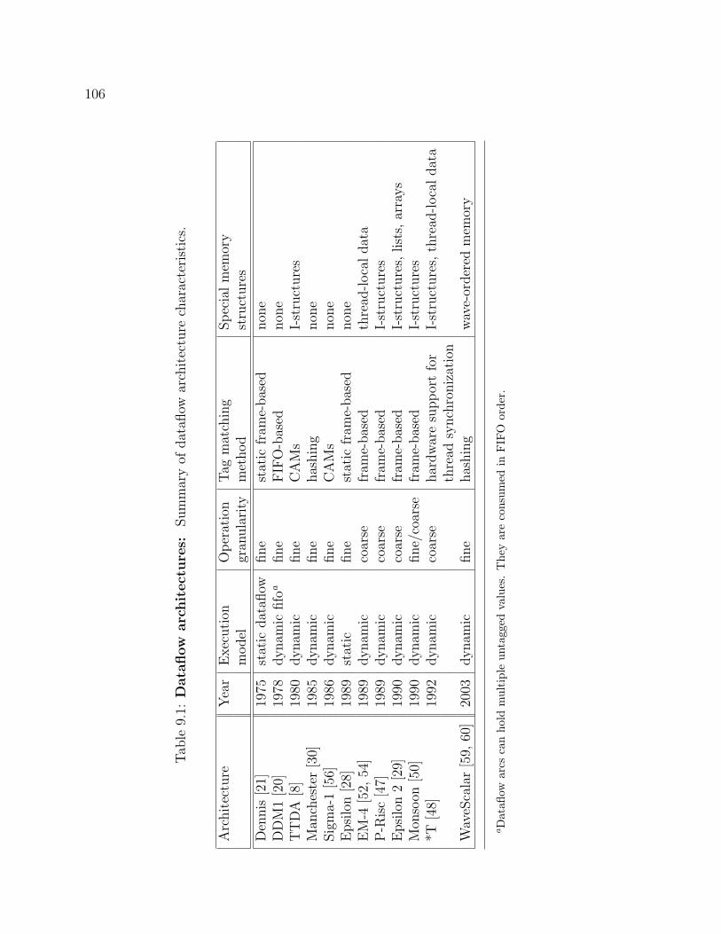
106
Tab
le9.
1:D
ata
flow
arc
hit
ectu
res:
Sum
mar
yof
dat
aflow
arch
itec
ture
char
acte
rist
ics.
Arc
hit
ectu
reYea
rE
xecu
tion
Oper
atio
nTag
mat
chin
gSpec
ialm
emor
ym
odel
gran
ula
rity
met
hod
stru
cture
s
Den
nis
[21]
1975
stat
icdat
aflow
fine
stat
icfr
ame-
bas
ednon
eD
DM
1[2
0]19
78dyn
amic
fifo
afine
FIF
O-b
ased
non
eT
TD
A[8
]19
80dyn
amic
fine
CA
Ms
I-st
ruct
ure
sM
anch
este
r[3
0]19
85dyn
amic
fine
has
hin
gnon
eSig
ma-
1[5
6]19
86dyn
amic
fine
CA
Ms
non
eE
psi
lon
[28]
1989
stat
icfine
stat
icfr
ame-
bas
ednon
eE
M-4
[52,
54]
1989
dyn
amic
coar
sefr
ame-
bas
edth
read
-loc
aldat
aP
-Ris
c[4
7]19
89dyn
amic
coar
sefr
ame-
bas
edI-
stru
cture
sE
psi
lon
2[2
9]19
90dyn
amic
coar
sefr
ame-
bas
edI-
stru
cture
s,list
s,ar
rays
Mon
soon
[50]
1990
dyn
amic
fine/
coar
sefr
ame-
bas
edI-
stru
cture
s*T
[48]
1992
dyn
amic
coar
sehar
dw
are
suppor
tfo
rI-
stru
cture
s,th
read
-loc
aldat
ath
read
synch
roniz
atio
nW
aveS
cala
r[5
9,60
]20
03dyn
amic
fine
has
hin
gw
ave-
order
edm
emor
y
aD
atafl
owar
csca
nho
ldm
ulti
ple
unta
gged
valu
es.
The
yar
eco
nsum
edin
FIF
Oor
der.

107
chines allow multiple values on an arc at once, allowing for both recursion and parallel
execution of loop iterations. The cost, however, comes in a more complicated dataflow
firing rule. Instead of waiting for any inputs to be available, operations must wait
until a set of matching inputs are available.
Dynamic dataflow machines di↵erentiate between instances of values by adding a
tag to each value. The combination of a data value and a tag is called a token. In
dynamic dataflow machines an operation can only execute if a set of tokens with the
same tag is present on its inputs. Normal operations copy the tag from the input
values to the outputs, but the instruction sets often provide special tag management
instructions to modify tags (i.e., WaveScalar’s Data-To-Wave and Wave-To-Data
instructions).
The MIT Tagged Token Dataflow Architecture (TTDA) [8] was one of the earliest
dynamic dataflow machines, and nearly all subsequent dataflow machines, including
WaveScalar, use the dynamic dataflow model. WaveScalar di↵ers from previous dy-
namic systems in providing a two-part tag (wave number and thread id) and giving
the programmer complete control over the tags. Previous machines provided special
hardware or firmware for automatic tag management.
Tag management increases the burden on the programmer slightly but allows
more flexible use of the available space of tags. For instance, the fine-grain threading
mechanism described in Section 8.1.1 relies upon creative use of wave number and
thread ids.
9.1.2 Operation granularity
In the abstract, the dataflow graph of an application defines a partial order over a set
of operations. Di↵erent dataflow models and their corresponding hardware implemen-
tations support di↵erent granularities of operation. Designs such as TTDA [8], the
Manchester machine [30], SIGMA-1 [56], Epsilon [28], Monsoon [50], and WaveScalar
used individual instructions as operations. Other designs, such as the EM4 [54, 52],
108
P-Risc [47], *T [48], and the Threaded Abstract Machine (TAM) [16] allowed for
coarse-grain operations (often called threads) and provided hardware acceleration for
synchronization operations.
The shift from fine-grained dataflow to coarse-grain dataflow was a response to
the high cost of frequent synchronization in fine-grain dataflow machines. Coarse-
grain operations make synchronization less frequent. They reduce communication
overhead, because each operation runs to completion on one processing element, con-
fining communication within an operation to a single processor.
Despite the strong trend in previous dataflow research toward coarse-grain op-
erations, WaveScalar uses fine-grain operations. The dataflow languages that older
dataflow machines targeted provide parallelism at a wide range of granularities. De-
signers could adjust the granularity of their operations to balance synchronization
and communication costs in the technology available at the time.
WaveScalar does not have this luxury, because one of its goals is to e�ciently
execute programs written in C. These programs tend to have a small amount of
instruction-level parallel (ILP) and, if they are multi-threaded, some very coarse-grain,
pthread-style parallelism. There is little or no parallelism in between. As a result,
WaveScalar must use fine-grain operations to exploit fine-grain ILP, so it uses di↵er-
ent techniques to address the costs of synchronization and communication, namely
careful instruction placement, a hierarchical interconnect, and a highly-optimized tag
matching scheme. WaveScalar’s hierarchical interconnect provides fast, local commu-
nication and our instruction placement scheme keeps most communication localized,
reducing communication costs. In addition, we apply a technique called k-loop bound-
ing [15] to reduce overflow and keep matching cheap.
9.1.3 Memory
Designers of the earliest dataflow machines intended them to run purely functional
languages that had no notion of mutable state. However, support for mutable state

109
can make programming some applications much easier. Many dataflow languages
incorporate some notion of mutable state along with special-purpose hardware to
make it fast.
Researchers have studied three di↵erent dataflow memory systems. We discuss I-
structures and M-structures below. Section 3.4.1 discusses the third approach, token-
passing.
I-structures Functional languages initialize variables when they are declared and
disallow modifying their values. This eliminates the possibility of read-after-write data
hazards: The variable always contains the correct value so any read is guaranteed to
see it. Dataflow language designers recognized that this approach restricts parallelism,
because an array must be completely initialized before its elements can be accessed.
Ideally, one thread could fill in the array while another thread accessed the initialized
elements.
Dataflow languages such Id [49] and SISAL [25] provide this ability with I-structures
[9]. I-structures are write-once memory structures. When a program allocates an I-
structure it is empty and contains no value. A program can write, or fill in, an
I-structure at most once. Reading from an empty I-structure blocks until the I-
structure is full. Reading from a full I-structure returns the value it holds. In the
array example above, one thread allocates an array of I-structures and starts filling
them in. The second thread can attempt to read entries of the array but will block if
it tries to access an empty I-structure.
M-structures M-structures [11] provide check-in/check-out semantics for variables.
Reading from a full M-structure removes the value, and a write fills the value back
in. Attempting to read from an empty M-structure blocks until the value is returned.
A typical example of M-structures in action is a histogram. Each bucket is an
M-structure, and a group of threads add elements to the buckets concurrently. Since

110
addition is commutative, the order of the updates is irrelevant, but they must be
sequentialized. M-structures provide precisely the necessary semantics.
Although I- and M-structures provide mutable state, they do not provide the
ordering semantics of imperative languages. Since WaveScalar must support these
languages, it provides wave-ordered memory. However, WaveScalar can emulate M-
structures using Thread-Coordinate.
9.1.4 Dataflow hardware
All dataflow machines follow a similar high-level design: A set of processing elements
(PEs) connected by some sort of interconnect. The individual PEs implement the
dataflow firing rule and execute instructions. Some designs also provides special I- or
M-structure processors to implement those constructs.
The individual PEs are typically pipelined. Tokens arrive at the top of the pipeline
and flow into a matching unit that checks whether the token completes a set of inputs
to a instruction. If it does, the instruction issues to the functional unit. Eventually,
the result of the operation leaves the pipeline and travels over the interconnect network
to its destination PE.
The most significant di↵erence among dataflow machines is how the matching units
implements the dataflow firing rule. Both static and dynamic machines must address
this issue because a processing element usually handles more than one instruction.
Static machines must check each value to see if it completes the set of inputs for an
instruction (i.e., if the destination instruction identifier matches the identifier of a
previously generated value). For dynamic machines the matching unit must check
both the destination instruction identifier and the tag. For fine-grained dataflow
architectures e�cient tag matching is crucial, but for coarse-grain designs it is less
frequent and, therefore, less important.
There are two main challenges. First, since the number of unconsumed input
tokens is potentially unbounded, the matching unit at each PE should be fast and
111
accommodate as many unconsumed input tokens as possible to minimize overflow.
Second, when overflow does occur, the architecture must provide a mechanism to
handle additional tokens. Research reports do not provide detailed descriptions of
overflow mechanisms, but the hope is that overflow is an infrequent occurrence.
Fine-grain dataflow architectures have used three techniques for tag matching:
associative search, hashing, frame-based lookup. We discuss each in turn.
Associative search The earliest dynamic dataflow machines [8] used associative
search. Special-purpose content-addressable memories (CAMs) check the tag of an
incoming token against all waiting tokens. CAMs are complex and require a great
deal of hardware to implement. This technique quickly fell from favor.
Hashing Architectures such as the Manchester machine [30] used hashing to re-
place expensive CAMs with conventional memories. As tokens arrive, the hardware
computes a hash of its tag and destination instruction identifier and uses the hash
to index into a memory. If the word of memory contains a matching token, a match
occurs and the instruction issues. If the word of memory contains a token with a
di↵erent tag, the hardware invokes an overflow mechanism. Finally, if the word of
memory is empty, the hardware places the new token there to await its matching
token. WaveScalar uses a hashing scheme. Section 4.2 describes it in detail.
Frame-based lookup Frame-based lookup, used in Monsoon [50] and EM-4 [54],
among others, relies on the compiler to eliminate the possibility of token overflow. The
compiler breaks the program into blocks (e.g., basic blocks, hyperblocks, or functions).
When the hardware needs to execute a block, it first allocates a frame of memory.
The frame contains one entry for each two-input instruction in the block (one-input
instructions do not need an entry because they do not require tag matching), and
each word of the frame carries a presence bit that denotes whether the entry is full or

112
empty. When an instruction generates a value, the hardware reads the frame entry
for the destination instruction. If the entry is full, a match occurs. Otherwise, the
hardware writes the new value into the frame entry to await its mate.
Static dataflow machines can be seen as frame-based machines in which a single
frame covers the entire program and only one frame is ever allocated. Dennis’s first
dataflow proposal [21] follows this approach.
9.2 Tiled architectures
The WaveCache hardware design in Chapters 4 and 5 is a tiled architecture. Broadly
speaking, a tiled architecture is a processor design that uses an array of basic building
blocks of silicon to construct a larger processor.
Tiled architectures provide three advantages over traditional monolithic designs.
First, they reduce design complexity by emphasizing design reuse. WaveScalar ex-
ploits this principle at several levels (PE, domain, and cluster). Second, tiled designs
seek to avoid long wires. In modern technology, wire delay dominates the cost of com-
putation. Wires in most tiled architectures span no more than a single tile, ensuring
that wire length does not increase with the number of tiles. Finally, tiled architec-
tures seek to be scalable. An ideal tiled architecture would scale to any number of
tiles both in terms of functional correctness and in terms of performance.
Several research groups have proposed tiled architectures with widely varying tile
designs. Smart Memories [42] provides multiple types of tiles (e.g., processing ele-
ments and reconfigurable memory elements). This approach allows greater freedom
in configuring an entire processor, since the mix of tiles can vary from one instanti-
ation to the next, perhaps avoiding the di�culties in naive scaling that we found in
our study.
The TRIPS [46, 53] processor uses dataflow ideas to build a hybrid von Neu-
mann/dataflow machine. The TRIPS processor uses a program counter to guide
execution, but instead of moving from one instruction to the next, the TRIPS PC

113
selects frames (similar to hyperblocks [41]) of instructions for execution in an array
of 16 processing elements that make up a TRIPS processor.
Despite high-level similarities between waves and frames and the WaveScalar and
TRIPS PE designs, the two architectures are quite di↵erent. In TRIPS, a register
file at the top of the array holds values that pass from one frame to another. Each
TRIPS PE can hold multiple instructions, so each PE requires multiple input bu↵ers.
However, execution follows the static dataflow model, making tag matching logic
unnecessary.
Using dataflow execution within a von Neumann processor is the same approach
taken by out-of-order superscalars, but the TRIPS design avoids the long wires and
broadcast structures that make conventional out-of-order processors non-scalable.
However, because it uses a program counter to select blocks of instructions for ex-
ecution, TRIPS must speculate aggressively. Mapping a frame of instructions onto
the PE array takes several cycles, so the TRIPS processor speculatively maps frames
onto the PEs ahead of time. WaveScalar does not su↵er from this problem because its
dynamic dataflow execution model allows instructions to remain in the grid for many
executions, obviating the need for speculation. The disadvantage of WaveScalar’s ap-
proach is the need for complex tag-matching hardware to support dynamic dataflow
execution
The two projects also have much in common. Both take a hybrid static/dynamic
approach to scheduling instruction execution by carefully placing instructions in an
array of processing elements and then allowing execution to proceed dynamically.
This places both architectures between extremely dynamic out-of-order superscalar
designs and fully statically scheduled VLIW machines. Those designs have run into
problems, because fully dynamic scheduling does not scale and static scheduling can
be very di�cult in practice. A hybrid approach will be necessary, but it is unclear
whether either WaveScalar or TRIPS strikes the optimal balance.
WaveScalar and TRIPS also take similar approaches to ordering memory opera-
114
tions. TRIPS uses load/store IDs (LSIDs) [57] to order memory operations within
a single frame. Like the sequence numbers in wave-ordered memory, LSIDs provide
ordering among the memory operations. However, the TRIPS scheme provides no
mechanism for detecting whether a memory operation will actually execute during
a specific dynamic execution of a frame. Instead, TRIPS guarantees that memory
operations that access the same address will execute in the correct order and modify
the consistency model to treat frames of instructions as atomic operations. LSID-
based memory ordering requires memory disambiguation hardware that increases the
complexity of the design relative to WaveScalar’s wave-ordering store bu↵er.
The RAW project [61] uses a simple processor core as a tile and builds a tightly-
coupled multiprocessor. The RAW processor provides for several di↵erent execution
models. The compiler can statically schedule a single program to run across all
the tiles, e↵ectively turning RAW into a VLIW-style processor. Alternatively, the
cores can run threads from a larger computation that communicate using RAW’s
tightly-integrate, inter-processor, message-passing mechanism. The former approach
is reminiscent of the coarse-grain dataflow processing described in Section 9.1.2.
The RAW project presents one vision for what an advanced CMP might look like,
and a careful study of its area-e�ciency would be worthwhile. One such study of
the RAW architecture [44] shares similar goals with ours (Section 7.2), but it takes a
purely analytical approach and creates models for both processor configurations and
applications. That study was primarily concerned with finding the optimal configu-
ration for a particular application and problem size, rather than a more universally
scalable, general purpose design.
9.3 Objections to dataflow
As Table 9.1 demonstrates, dataflow processors fell out of favor between the early
1990’s and the early twenty-first century. Several factors contributed to this, including
cheaper, higher-performance commodity processors and the integration of dataflow
115
ideas into out-of-order processors. But there was also a feeling that dataflow was
flawed as an execution model, at least given the technology available at the time.
Culler [17] articulated the di�culties with dataflow as two key problems. First,
the memory hierarchy limits the amount of latency a dataflow machine can hide.
A processor can only hide latency (and keep busy) by executing instructions whose
inputs are at the top level of the memory hierarchy. If the top of the memory hierarchy
is too small, the processor will sit idle, waiting for the inputs to arrive.
Second, the dataflow firing rule is naive, since it ignores locality in execution.
Ideally, a dataflow machine would execute program fragments that are related to
one another to exploit locality and prevent “thrashing” at the top of the memory
hierarchy.
Culler’s first argument does not apply to WaveScalar because of changes in tech-
nology. The relatively small number of transistors available on a single die in the
early 1990’s meant that execution resources were expensive. As a result hiding la-
tency and keeping the processors busy were the keys to performance. Things have
changed significantly. WaveScalar sidesteps the need to keep many data values “near”
a handful of processing elements by building many processing elements, each with a
small amount of nearby memory for storing unmatched tokens.
WaveScalar’s carefully-tuned placement system addresses the problems with lo-
cality and scheduling. As described in Section 4.6 the placement algorithm attempts
to schedule dependent instructions on a single PE, ensuring that a large fraction
(30-40%) of message tra�c occurs within a single pod. This reduces the need for
bu↵ering a large number of tokens because, tokens tend to be consumed shortly af-
ter they are produced. In addition, k-loop bounding reduces the frequency of token
overflow, further improving locality.

116
Chapter 10
CONCLUSIONS AND FUTURE WORK
The WaveScalar instruction set, execution model, and hardware architecture demon-
strate that dataflow computing is a viable alternative to the von Neumann model.
WaveScalar overcomes the limitations of previous dataflow architectures, addresses
many of the challenges that modern processors face, exploits many types of paral-
lelism, and provides high performance on a wide range of applications.
WaveScalar makes two key contributions to dataflow instruction sets. The first is
wave-ordered memory. By adding a simple set of annotations, WaveScalar provides
the sequential memory semantics that imperative programming languages require
without destroying the parallelism that the dataflow model expresses. Without wave-
ordered memory, or a scheme like it, dataflow processing has little chance of being a
viable competitor to von Neumann processors.
Work on wave-ordered memory is not complete, and two key areas remain to be
explored. The evaluation in Chapter 3 uses our binary translator-based toolchain, and
the binary translator cannot make full use of wave-ordered memory. In particular, it
does not have access to good aliasing information or high-level structural information
about the program. Better aliasing knowledge would allow for more aggressive use of
the ripple annotation (and the unordered memory interface, see below), and structural
information would allow the compiler to generate larger, more e�cient waves. Work
in these directions is underway.
More broadly, wave-ordered memory demonstrates the value of encoding pro-
gram structure explicitly in the instruction set. This idea has applications beyond
WaveScalar or even dataflow processing. Extending conventional instruction sets to

117
encode more information about program behavior, control structure, or memory usage
is one approach to improving performance in the face of stringent technological con-
straints. The challenge is finding concise, flexible ways to express useful information
to the processor.
WaveScalar’s second contribution to dataflow instruction sets is its ability to com-
bine the imperative memory semantics that wave-ordered memory provides with
the massive amounts of parallelism that a dataflow execution model can express.
WaveScalar’s unordered memory interface provides the means to exploit this type
of parallelism among memory operations, while providing well-defined semantics for
combining ordered and unordered accesses in the same program.
In addition to intermingling accesses via the ordered and unordered memory in-
terfaces, WaveScalar also allows the programmer to combine coarse- and fine-grain
threading styles to express a range of di↵erent types of parallelism. The combination
of two threading models and two memory interfaces provides WaveScalar program-
mers with enormous flexibility in expressing parallelism. This leads to better perfor-
mance, but it also has the potential to ease the burden on programmers, because they
can express the types of parallelism that are most natural in the program at hand.
Fully realizing this goal will require additional work, however. Currently the only
way to exploit the fine-grain threading and unordered memory is via hand-written
dataflow assembly (a di�cult undertaking). Ongoing compiler work aims to apply
both interfaces to single-threaded codes automatically. Other approaches include
porting a compiler for a dataflow programming language to WaveScalar or extending
an imperative language to support these interfaces explicitly.
The WaveScalar hardware architecture in Chapters 4 and 5 is designed to be scal-
able and of low complexity, and to e↵ectively exploit the di↵erent types of parallelism
the WaveScalar ISA can express. Our WaveScalar design reduces design complexity
by combining identical components hierarchically. This approach reduces the amount
of hardware that must be designed and verified. It also eases the impact of manufac-
118
turing defects. If a portion of the chip, for instance a PE, is manufactured incorrectly,
that PE can be disabled without significantly impacting the rest of the chip. Investi-
gating what kinds of manufacturing errors the WaveScalar architecture can tolerate
and how it would adapt to them is the subject of future work.
To evaluate WaveScalar we used a combination of RTL synthesis (for area and
delay measurements) and cycle-level simulation (for performance measurements). Our
results are encouraging. An exhaustive search of WaveScalar’s design space reveals
that the WaveScalar processor is scalable. For chip sizes from 39mm2 to 294mm2, it
scales almost perfectly, realizing a 6.4-fold increase in performance for a 7.5⇥ increase
in chip area. We also found that the most area-e�cient single-cluster design scales to
the most e�cient 4- and 16-cluster designs.
Eventually, we plan to extend this to include power in addition to area and per-
formance. Synthesis tools can extract power consumption estimates from our RTL
model, and by combining these with event counts from our simulator, we can compute
WaveScalar’s power requirements. Using this infrastructure, we can evaluate di↵er-
ent approaches to power management in a WaveScalar processor, including clock- and
power-gating at the PE, domain, and cluster levels as well as power-aware instruc-
tion placement. Including power will also force us to carefully consider aspects of
the design like the interconnect that have little impact on area, but might contribute
significantly to the power budget.
We will also extend the study to include a wider range of applications. Currently,
the limitations of our toolchain and runtime environment prevent us from running
large-scale “commercial” workloads that would put significantly more pressure on the
memory system and the WaveScalar’s instruction capacity than our current suite of
applications. Running these workloads on WaveScalar will lead to further refinements
in the architecture. For instance, our current cache coherence protocol contains only
simple optimizations for migratory sharing, because preliminary limit studies showed
that for our applications the benefits of more complicated schemes were small. For

119
applications with threads that span several clusters and have more inter-thread com-
munication, a more sophisticated scheme might perform better.
Using the scalable design points from our pareto analysis, we compared WaveScalar
to more conventional architectures. Our results show that a well-tuned WaveScalar
design outperforms more conventional CMP designs on multi-threaded workloads by
between 2⇥ and 11⇥ depending on the workload, and it achieves single-threaded
performance similar to that of an aggressive out-of-order superscalar but in 30% less
area.
The results for WaveScalar’s fine-grain threading and unordered memory interfaces
are even more encouraging. For kernels, these interfaces can provide speedups of
between 16⇥ and 240⇥. When both memory interfaces and both threading styles are
brought to bear (something that is impossible in a conventional CMP), they increased
overall performance by 9⇥ for one application.
WaveScalar demonstrates that dataflow computing is a viable alternative to con-
ventional von Neumann processing. More important, however, are questions of order,
parallelism, distributed control, and scalability that this work has explored. These
problems are at the heart of one of the central challenges facing computer system
designers today: How can we design and build computer systems that are both easy
to implement and will deliver performance that scales with technology? This thesis
used WaveScalar to begin addressing this question.
120
BIBLIOGRAPHY
[1] Cadence website. http://www.cadence.com.
[2] Synopsys website. http://www.synopsys.com.
[3] TCB013GHP - TSMC 0.13um core library. Taiwan Semiconductor Manufactur-ing Company, Ltd. Release 1.0. October 2003.
[4] S. V. Adve and K. Gharachorloo. Shared memory consistency models: a tutorial.IEEE Computer, 29(12), December 1996.
[5] V. Agarwal, M. S. Hrishikesh, S. W. Keckler, and D. Burger. Clock rate versusIPC: The end of the road for conventional microarchitectures. In Proceedings ofthe 27th Annual International Symposium on Computer Architecture, 2000.
[6] J. M. Arnold, D. A. Buell, and E. G. Davis. Splash 2. In Proceedings of the 4thSymposium on Parallel Algorithms and Architectures, 1992.
[7] Arvind. Dataflow: Passing the token. 32nd Annual International Symposium onComputer Architecture Keynote, June 2005.
[8] Arvind and R.S. Nikhil. Executing a program on the MIT tagged-token dataflowarchitecture. IEEE Transactions on Computers, 39(3):300–318, 1990.
[9] Arvind, R.S. Nikhil, and K. K. Pingali. I-structures: Data structures for par-allel computing. ACM Transaction on Programming Languages and Systems,11(4):598–632, 1989.
[10] L. A. Barroso, K. Gharachorloo, R. McNamara, A. Nowatzyk, S. Qadeer,B. Sano, S. Smith, R. Stets, and B. Verghese. Piranha: A scalable architec-ture based on single-chip multiprocessing. In Proceedings of the 27th AnnualInternational Symposium on Computer Architecture, 2000.
[11] P. S. Barth, R. S. Nikhil, and Arvind. M-structures: Extending a parallel, non-strict, functional languages with state. Technical Report MIT/LCS/TR-327,MIT, 1991.
121
[12] M. Beck, R. Johnson, and K. Pingali. From control flow to data flow. Journalof Parallel and Distributed Computing, 12:118–129, 1991.
[13] M. Budiu, G. Venkataramani, T. Chelcea, and S. C. Goldstein. Spatial compu-tation. SIGPLAN Notices, 39(11):14–26, 2004.
[14] D. Chinnery and K. Keutzer. Closing the Gap Between ASIC & Custom. KluwerAcademic Publishers, 2003.
[15] D. E. Culler. Managing Parallelism and Resources in Scientific Dataflow Pro-grams. PhD thesis, Massachusetts Institute of Technology, March 1990.
[16] D. E. Culler, A. Sah, K. E. Schauser, T. Eicken, and J. Wawrzynek. Fine-grainparallelism with minimal hardware support: A compiler-controlled threaded ab-stract machine. In Proceedings of the 4th International Conference on Architec-tural Support for Programming Languages and Operating Systems, 1991.
[17] D. E. Culler, K. E. Schauser, and T. von Eicken. Two fundamental limits ondataflow multiprocessing. In Proceedings of the IFIP WG 10.3 Working Confer-ence on Architectures and Compilation Techniques for Fine and Medium GrainParallelism, 1993.
[18] R. Cytron, J. Ferrante, B. K. Rosen, M. N. Wegman, and F. K. Zadeck. E�cientlycomputing static single assignment form and the control dependence graph. ACMTransactions on Programming Languages and Systems, 13(4):451–490, 1991.
[19] W. J. Dally and C. L. Seitz. Deadlock-free message routing in multiprocessor in-terconnection networks. IEEE Transactions on Computing, 36(5):547–553, 1987.
[20] A. L. Davis. The architecure and system method of DDM1: A recursively struc-tured data driven machine. In Proceedings of the 5th Annual Symposium onComputer Architecture, 1978.
[21] J. B. Dennis. A preliminary architecture for a basic dataflow processor. InProceedings of the 2nd Annual Symposium on Computer Architecture, 1975.
[22] J. B. Dennis. First version data flow procedure language. Technical Report MACTM61, MIT Laboratory for Computer Science, May 1991.
[23] R. Desikan, D.C. Burger, S.W. Keckler, and T.M. Austin. Sim-alpha: A val-idated, execution-driven Alpha 21264 simulator. Technical Report TR-01-23,UT-Austin Computer Sciences, 2001.
122
[24] M. Ekman and P. Stenstrom. Performance and power impact of issue widthin chip-multiprocessor cores. In Proceedings of the International Conference onParallel Processing, 2003.
[25] J. T. Feo, P. J. Miller, and S. K. Skedzielewski. SISAL90. In Proceedings of HighPerformance Functional Computing, 1995.
[26] S. C. Goldstein and M. Budiu. NanoFabrics: Spatial computing using molecu-lar electronics. In Proceedings of the 28th Annual International Symposium onComputer Architecture, 2001.
[27] J. R. Goodman, M. K. Vernon, and P. J. Woest. E�cent synchronization prim-itives for large-scale cache-coherent multiprocessors. In Proceedings of the 3rdInternational Conference on Architectural Support for Programming Languagesand Operating Systems, 1989.
[28] V. G. Grafe, G. S. Davidson, J. E. Hoch, and V. P. Holmes. The Epsilon dataflowprocessor. In Proceedings of the 16th Annual International Symposium on Com-puter Architecture, 1989.
[29] V.G. Grafe and J.E. Hoch. The Epsilon-2 hybrid dataflow architecture. InProceedings of the 35th IEEE Computer Society International Conference, 1990.
[30] J. R Gurd, C. C Kirkham, and I. Watson. The Manchester prototype dataflowcomputer. Communications of the ACM, 28(1):34–52, 1985.
[31] L. Hammond, B.A. Hubbert, M. Siu, M.K. Prabhu, M. Chen, and K. Olukolun.The Stanford Hydra CMP. IEEE Micro, 20, March/April 2000.
[32] M. S. Hrishikesh, D. Burger, N. P. Jouppi, S. W. Keckler, K. I. Farkas, andP. Shivakumar. The optimal logic depth per pipeline stage is 6 to 8 FO4 inverterdelays. In Proceedings of the 29th Annual International Symposium on ComputerArchitecture, 2002.
[33] A. Jain, W. Anderson, T. Benningho↵, and D. E. Berucci. A 1.2GHz Alphamicroprocessor with 44.8GB/s chip pin bandwidth. In Proceedings of the IEEEInternational Solid-State Circuits Conference, 2001.
[34] S. W. Keckler, W. J. Dally, D. Maskit, N. P. Carter, A. Chang, and W. SingLee. Exploiting fine-grain thread level parallelism on the MIT multi-ALU proces-sor. In Proceedings of the 26nd Annual International Symposium on ComputerArchitecture, 1998.

123
[35] M. Kishi, H. Yasuhara, and Y. Kawamura. DDDP-a distributed data driven pro-cessor. In Proceedings of the 10th Annual International Symposium on ComputerArchitecture, 1983.
[36] K. Krewel. Alpha EV7 processor: A high-performance tradition continues. Mi-croprocessor Report, April 2005.
[37] J. Laudon. Performance/watt: the new server focus. SIGARCH Computer Ar-chitecture News, 33(4):5–13, 2005.
[38] C. Lee, M. Potkonjak, and W. H. Mangione-Smith. Mediabench: A tool for eval-uating and synthesizing multimedia and communicatons systems. In Proceedingsof the 30th Annual International Symposium on Microarchitecture, 1997.
[39] W. Lee, R. Barua, D. Srikrishna, J. Babb, V. Sarkar, and S. Amarasinghe.Space-time scheduling of instruction-level parallelism on a RAW machine. InProceedings of the 8th Annual International Conference on Architectural Supportfor Programming Languages and Operating Systems ASPLOS-VIII, 1998.
[40] J. L. Lo, J. S. Emer, H. M. Levy, R. L. Stamm, D. M. Tullsen, and S. J. Eggers.Converting thread-level parallelism to instruction-level parallelism via simulta-neous multithreading. ACM Transactions on Computer Systems, 15(3):322–354,1997.
[41] S. A. Mahlke, D. C. Lin, W. Y. Chen, R. E. Hank, and R. A. Bringmann. E↵ectivecompiler support for predicated execution using the hyperblock. In Proceedingsof the 25th Annual International Symposium on Microarchitecture, 1992.
[42] K. Mai, T. Paaske, N. Jayasena, R. Ho, W. J. Dally, and M. Horowitz. SmartMemories: a modular reconfigurable architecture. In Proceedings of the 27thAnnual International Symposium on Computer Architecture, 2000.
[43] M. Mercaldi, M. Oskin, and S. E. Eggers. A performance model to guide in-struction scheduling on spatial computers. In submission to the Symposium onParallel Algorithms and Architectures”.
[44] C. A. Moritz, D. Yeung, and A. Agarwal. Exploring performance-cost optimaldesigns for RAW microprocessors. In Proceedings of the International IEEESymposium on Field-Programmable Custom Computing Machines, 1998.
124
[45] S. S. Mukherjee, C. Weaver, J. Emer, S. K. Reinhardt, and T. Austin. A system-atic methodology to compute the architectural vulnerability factors for a high-performance microprocessor. In Proceedings of the 36th Annual InternationalSymposium on Microarchitecture, 2003.
[46] R. Nagarajan, K. Sankaralingam, D. Burger, and S. Keckler. A design spaceevaluation of grid processor architectures. In Proceedings of the 34th AnnualInternational Symposium on Microarchitecture, 2001.
[47] R. S. Nikhil and Arvind. Can dataflow subsume von Neumann computing? InProceedings of the 16th Annual International Symposium on Computer Architec-ture, 1989.
[48] R. S. Nikhil, G. M. Papadopoulos, and Arvind. *T: A multithreaded massivelyparallel architecture. In Proceedings of the 19th Annual International Symposiumon Computer Architecture, 1992.
[49] R.S. Nikhil. The parallel programming language Id and its compilation for paral-lel machines. In Proceedings of the Workshop on Massive Paralleism: Hardware,Programming and Applications, 1990.
[50] G. M. Papadopoulos and D. E. Culler. Monsoon: an explicit token-store architec-ture. In Proceedings of the 17th Annual International Symposium on ComputerArchitecture, 1990.
[51] G. M. Papadopoulos and K. R. Traub. Multithreading: A revisionist view ofdataflow architectures. In Proceedings of the 18th Annual International Sympo-sium on Computer Architecture, 1991.
[52] S. Sakai, Y. Yamaguchi, K. Hiraki, Y. Kodama, and T. Yuba. An architecture ofa dataflow single chip processor. In Proceedings of the 16th Annual InternationalSymposium on Computer Architecture, 1989.
[53] K. Sankaralingam, R. Nagarajan, H.Liu, C. Kim, J. Huh, D. Burger, S. W. Keck-ler, and C. R. Moore. Exploiting ILP, TLP, and DLP with the polymorphousTRIPS architecture. In Proceedings of the 30th Annual International Symposiumon Computer Architecture, 2003.
[54] M. Sato, Y. Kodama, S. Sakai, Y. Yamaguchi, and Y. Koumura. Thread-basedprogramming for the EM-4 hybrid dataflow machine. In Proceedings of the 19thAnnual International Symposium on Computer Architecture, 1992.

125
[55] T. Shimada, K. Hiraki, and K. Nishida. An architecture of a data flow machienand its evaluation. In COMPCON Digest of Papers, 1984.
[56] T. Shimada, K. Hiraki, K. Nishida, and S. Sekiguchi. Evaluation of a prototypedata flow processor of the SIGMA-1 for scientific computations. In Proceedingsof the 13th Annual International Symposium on Computer Architecture, 1986.
[57] A. Smith, J. Gibson, B. Maher, N. Nethercote, B. Yoder, D. Burger, K. S.McKinley, and J. Burrill. Compiling for EDGE architectures. In Proceedings ofthe International Symposium on Code Generation and Optimization, 2006.
[58] SPEC. SPEC CPU 2000 benchmark specifications, 2000. SPEC2000 BenchmarkRelease.
[59] S. Swanson, K. Michelson, A. Schwerin, and M. Oskin. WaveScalar. In Proceed-ings of the 36th Annual International Symposium on Microarchitecture, 2003.
[60] S. Swanson, A. Putnam, K. Michelson, M. Mercaldi, A. Petersen, A. Schw-erin, M. Oskin, and S. J. Eggers. Area-performance trade-o↵s in tiled dataflowarchitectures. In Proceedings of the 33rd Annual International Symposium onComputer Architecture, 2006.
[61] M. B. Taylor, W. Lee, J. Miller, D. Wentzla↵, I. Bratt, B. Greenwald, H. Ho↵-mann, P. Johnson, J. Kim, J. Psota, A. Saraf, N. Shnidman, V. Strumpen,M. Frank, S. Amarasinghe, and A. Agarwal. Evaluation of the RAW micropro-cessor: An exposed-wire-delay architecture for ILP and streams. In Proceedingsof the 31st Annual International Symposium on Computer Architecture, 2004.
[62] D. Tullsen, J. Lo, S. Eggers, and H. Levy. Supporting fine-grain synchronizationon a simultaneous multithreaded processor. In Proceedings of the 5th AnnualInternational Symposium on High Performance Computer Architecture, 1999.

126
VITA
Steven Swanson was born and raised in Pocatello, Idaho, but he currently lives
in Seattle. He earned a Bachelor of Science in Computer Science and Mathematics
at the University of Puget Sound in Tacoma, Washington in 1999 and a Master of
Science in Computer Science and Engineering from the University of Washington in
2001. In 2006, he earned a Doctor of Philosophy at the University of Washington in
Computer Science and Engineering.