The Welfare Effects of Eviction and HomelessnessPolicies*

Boaz Abramson

Department of Economics

Stanford University

boaza@stanford.edu

November 21, 2021

[Link to most updated version]

Abstract

This paper studies the implications of rental market policies that address evictions and

homelessness. Policies that make it harder to evict delinquent tenants, for example

by providing tax-funded legal counsel in eviction cases (“Right-to-Counsel”) or by

instating eviction moratoria, protect renters from eviction in bad times. However,

higher default costs to landlords lead to higher equilibrium rents and lower housing

supply, implying homelessness might increase. I quantify these tradeoffs in a model of

rental markets in a city, matched to micro data on rents and evictions as well as shocks

to income and family structure. I find that “Right-to-Counsel” drives up rents so

much that homelessness increases by 15% and welfare is dampened. Since defaults on

rent are driven by persistent income shocks, making it harder to evict tends to extend

the eviction process but doesn’t prevent evictions. In contrast, rental assistance lowers

tenants’ default risk and as a result reduces homelessness by 45% and evictions by

75%. It increases welfare despite its costs to taxpayers. Eviction moratoria following

an unexpected economic downturn can also prevent evictions and homelessness, if

used as a temporary measure.

JEL CODES: E60,G10,R30

*For invaluable guidance I thank Monika Piazzesi and Martin Schneider. I have also benefited fromhelpful suggestions by Ran Abramitzky, Adrien Auclert, Luigi Bocola, Rebecca Diamond, Liran Einav, JesusFernandez-Villaverde, Bob Hall, Patrick Kehoe, Pete Klenow, Sean Myers, Chris Tonetti, Alessandra Voena,Joakim Weill (discussant), and Andres Yany, as well as participants of the Stanford Macro Seminar and the15th North American Meeting of the Urban Economics Association. I acknowledge financial support fromthe Stanford Institute for Economic Policy Research. Any errors are my own.

1 Introduction

Across the US, approximately 2.2 million eviction cases are filed against renters every year(Desmond et al., 2018) and 600, 000 people sleep on the streets or in homeless shelters ina given night.1 A growing body of research documenting the negative outcomes asso-ciated with housing insecurity has triggered a public debate over policies that addressevictions and homelessness. Policymakers across the country have considered enactingstronger tenant protections against evictions, for example by providing free legal counselin eviction cases (“Right-to-Counsel”), or by instating eviction moratoria. Rental assis-tance programs are also often proposed as a tool for reducing housing insecurity. Whilethese policies provide protections against evictions and homelessness, they can also affectequilibrium rents and the supply of rental units.

In this paper, I study the welfare effects of these policies. To this end, I propose adynamic equilibrium model of the rental market that explicitly allows for evictions andhomelessness. On the one hand, policies that make it harder to evict tenants who defaulton rent, like “Right-to-Counsel”, protect renters from the costs of eviction in bad times.On the other hand, they lead to higher equilibrium rents and lower housing supply asthey increase the costs of default for landlords. This means that homelessness can increaseif more households cannot afford to sign rental leases in the first place. I quantify themodel to data on evictions, homelessness, and rents in the San Diego metro area. My firstfinding is that “Right-to-Counsel” drives up rents so much that it increases homelessnessand lowers welfare. The most important new fact that the model matches, and that leadsto the overall negative evaluation of “Right-to-Counsel”, is that the income shocks thatdrive tenants to default are persistent in nature. When risk is persistent, making it harderto evict is ineffective in preventing evictions of delinquent renters, because these tenantscontinue defaulting until they are eventually evicted.

I provide evidence on the persistent nature of risk that drives defaults on rent by draw-ing on novel micro data on evictions. Starting with survey evidence on why tenants getevicted, I show that the main risk factors leading to defaults are job-loss and divorce.Using income data, I then show that these events are in fact associated with persistentdrops in income. Furthermore, by linking the universe of eviction cases in San Diego toa registry of individual address histories that records demographic characteristics fromInfutor, I show that tenants who are at a higher risk to default on rent, namely the youngand poor, are indeed more exposed to job-loss and divorce risk. I proceed to estimate an

1According to Point-in-Time counts published by the US Department of Housing and Urban Develop-ment (HUD), see https://www.hudexchange.info/programs/hdx/pit-hic/.

1

income process that fits these facts and that serves as a key input to the model.In contrast to “Right-to-Counsel”, I find that means-tested rental assistance is a promis-

ing solution to the housing insecurity crisis. The main conceptual difference is that rentalassistance lowers the likelihood that tenants default in the first place, as opposed to mak-ing it harder to evict tenants who have already defaulted. Indeed, rental assistance re-duces evictions and homelessness and improves welfare, despite its monetary costs. Infact, my estimates for San Diego suggest that the externality cost that homelessness im-poses on the city is so high that rental assistance more than pays for itself: the savingsin terms of expenditure on homelessness outweigh the cost of subsidizing rent. Finally,I find that an eviction moratorium following an unexpected aggregate unemploymentshock can prevent evictions and homelessness along the transition path, as long as it isused as a temporary measure, and is lifted before rents can adjust.

At the heart of the model are overlapping generations of households who have pref-erences over numeraire consumption and housing services and face idiosyncratic incomeand divorce risk. Households rent houses from real-estate investors by signing long-termleases that are non-contingent on future states. Namely, a lease specifies a per-period rentwhich is fixed for the duration of the lease. To move into the house, a household mustpay rent in the same period in which the lease begins, but a key feature of the model isthat in subsequent periods households may default on rent. Defaults on rent happen inequilibrium because contracts are non-contingent and because households are borrow-ing constrained. When a household begins to default, for example due to a bad incomeshock, an eviction case is filed against it. The eviction case extends until the householdgets evicted or until it stops defaulting.

Each period in which the household defaults, it is evicted with an exogenous prob-ability that captures the strength of tenant protections against evictions in the city. Ahousehold who defaults but is not evicted lives in the house for free for the durationof the period, and accrues rental debt into the next period. Households with outstand-ing debt from previous periods can either repay the debt they owe, in addition to theper-period rent, or they can continue to default and face a new draw of the eviction re-alization. Guided by recent evidence on the consequences of eviction (e.g. Humphrieset al., 2019), I model the cost of eviction as consisting of three components: temporaryhomelessness, partial repayment of outstanding debt, and a deadweight penalty on re-maining wealth that captures, among others, health deterioration and material hardshipthat follow eviction. Evictions are costly for society both because they impose a wealthloss for individuals, and because they lead to homelessness, which imposes an externalitycost in terms of expenditure to a local government. The government finances the cost of

2

homelessness through a lump-sum tax on investors.Real-estate investors buy houses in the housing market and rent them to households.

In addition to the cost of buying a house, investors incur a per-period maintenance costwhich has to be paid regardless of whether or not their tenant defaults. Thus, from theinvestor perspective, rental leases are long-duration risky assets. Investors observe someof the household’s characteristics at the period in which the lease begins, and are assumedto price the per-period rent in a risk-neutral manner, such that for each lease they breakeven in expectation. Equilibrium rents can then be thought of as equal to a risk-free rentplus a default premia that reflects the costs of default on rent to investors. Houses areindivisible and are inelastically supplied by landowners. Production of houses is subjectto a minimal quality constraint, reflecting minimal habitability laws. Households thatcannot afford to pay the first period’s rent on the lowest quality house become homeless,which is costly for the city.

The model allows for a discussion of the major policies that are proposed to reduceevictions and homelessness. A common goal of these policies is to provide protectionsagainst evictions and homelessness. One way this is done is by making it harder to evictdelinquent tenants, which in the model is captured by a lower likelihood of eviction givendefault. On the one hand, this can be welfare improving as it can prevent costly evictionsand homelessness. On the other hand, landlords pass the cost of insurance on to house-holds in the form of higher default premia, which implies that more households cannotafford to move into the lowest quality house. Thus, overall homelessness can increase.Quantitatively, the nature of risk that drives defaults on rent is key for assessing thistrade-off. When risk is persistent, making it harder to evict is less effective in preventingevictions and homelessness because delinquent tenants are likely to continue defaultinguntil they are eventually evicted.

A second way to protect tenants is by providing rental assistance, which is modeledas means-tested transfers that must be used to pay rent. On the one hand, rental assis-tance lowers the likelihood that tenants default on rent and face eviction, and it preventspoor households from becoming homeless by subsidizing their rent. This lowers the ex-ternality costs of homelessness. On the other hand, rental assistance is expensive, and inequilibrium the government might need to impose higher taxes on investors. Moreover,as demand for rentals increases, housing supply and house prices also rise to equilibratethe market. This implies that the risk-free rent, which partly reflects the price of buying ahouse for investors, is also higher, such that renters without default risk face higher equi-librium rents. This highlights an important general principle of the model, which is thatrental market policies affect not only poor households, but also richer renters through

3

their effect on the equilibrium risk-free rent.I quantify the model to the San Diego-Carlsbad-San-Marcos MSA, where homeless-

ness is a major problem and high-quality eviction data are available. The quantificationrequires not only the estimated income process, but also the parameters of the evictionregime, the externality cost of homelessness, and preferences and housing technology pa-rameters. I exploit detailed eviction court data from San Diego to identify the evictionregime parameters. The likelihood of eviction given default is identified by the averagelength of the eviction process, and the garnishment parameter governing debt repaymentupon eviction is identified from the share of debt collected by landlords. I estimate thecity’s per-household expenditure on homelessness using an external report on the cost ofhomelessness to San Diego County.

I jointly estimate parameters that govern preferences and housing technology usinga Simulated Method of Moments (SMM) approach. The estimation successfully matchesfacts on homelessness, evictions, rents and house prices in San Diego. In particular, Iestimate the minimal house quality such that the average rent in the bottom housingsegment matches the average rent in the bottom quartile of rents in San Diego. I identifythe (dis)utility from homelessness from the homelessness rate in San Diego. The wealthpenalty associated with eviction is identified from the eviction filing rate, which is definedas the share of renter households who face an eviction case during the year.

As a check of the model’s quantification, I evaluate its fit to non-targeted moments.First, I show that the model accounts for how eviction risk varies in the cross section ofrenters within San Diego. The model matches the disproportionately high eviction fil-ing rates for young renters as well as the general downward trend across ages. It alsodoes well in matching the share of eviction filings that are related to divorces. The modelgenerates these patterns because, consistent with the data, young renters are poorer andare more likely to lose their job and get divorced, and because divorce itself is associatedwith elevated income risk. Second, the model is consistent with the negative empirical re-lationship between rent burden and household income, which is of particular importancefor studying housing insecurity. In the model, this is driven by the minimal house qualityconstraint which limits the ability of poor households to lower their rent spendings.

Consistent with the empirical evidence on the persistent nature of risk that drives ten-ants to default on rent, I find that the vast majority of defaults in the model are instigatedby persistent income shocks. In particular, 68% of default spells begin with a negativepersistent income shock, 30% are due to a combination of a negative persistent shock anda negative transitory shock, and only 2% are driven by a transitory shock alone. In thispersistent risk environment, shocks cannot easily be smoothed across time, and there is

4

limited scope for preventing evictions by making it harder to evict delinquent tenants.I use the quantified model to evaluate the main policies that are proposed for reducing

housing insecurity. First, I study the effects of a “Right-to-Counsel” reform. To do so, Iexploit micro level evidence on how legal counsel makes it harder and more costly forlandlords to evict delinquent tenants. The “Shriver Act”, an RCT conducted in San Diegoby the Judicial Council of California, finds that lawyers prolong the eviction process byapproximately two weeks and lower debt repayments by 15% (Judicial Council of Cali-fornia, 2017). These estimates identify the parameters of a counterfactual eviction regimeassociated with “Right-to-Counsel”, where all tenants facing evictions are representedby lawyers. Namely, under this regime, the likelihood of eviction given default and theshare of debt that evicted tenants pay their landlord are lower. To evaluate the equilib-rium effects of a city-wide “Right-to-Counsel” reform, when rents and housing supplycan adjust, I compute the new steady state under this more lenient eviction regime.

The main result is that “Right-to-Counsel” drives up default premia so much thathomelessness increases by 15 percent. Evictions are lower, but this is mainly because poorhouseholds, who are initially at a higher risk of default and eviction, are priced out of therental market altogether. In particular, lawyers are unsuccessful in preventing evictionsof delinquent tenants: the share of eviction cases that are resolved with an eviction (asopposed to repayment of debt) is nearly one in the baseline economy, and is only slightlylower under “Right-to-Counsel”. Since defaults are mostly driven by persistent shocks,tenants who default on rent are unlikely to be able to repay their debt in the future, evenif they have longer periods of time to do so. This result highlights that the evaluation oftenant protections should take into account not only the effect on evictions, but also onhousing affordability and homelessness.

“Right-to-Counsel” has interesting distributional effects through its effect on housingsupply and risk-free rents. As default premia increase, some middle-income renters areforced to downgrade from upper to lower quality housing segments. In equilibrium,housing supply and the house price decline in the upper segments. The risk-free rent,which partly reflects the cost of buying a house for investors, therefore falls in these seg-ments. Rich renters in the upper segments with zero default risk then face lower rentsin equilibrium, and are in fact better off under the policy. In contrast, welfare losses areparticularly large for poor households who are pushed into homelessness. Overall, I findthat “Right-to-Counsel” dampens aggregate welfare. Furthermore, the annual cost of pro-viding legal counsel is 7.3 million dollars, and the increase in homelessness imposes anadditional expenditure of 30 million dollars to San Diego County every year.

The second policy I evaluate is a means-tested rental assistance program. In particular,

5

I consider subsidizing $400 of monthly rent to households with income and savings be-low a threshold of $1, 000. The main conceptual difference relative to “Right-to-Counsel”is that rental assistance lowers the likelihood that tenants default on rent, rather thanmaking it harder to evict those who have already defaulted. Indeed, I find that this pol-icy reduces homelessness by 45% and the eviction filing rate by 75%. Poor householdsare more likely to afford to move into a house both because the government subsidizestheir rent, and because the insurance provided by the subsidy lowers default premia inequilibrium. Evictions drop because the subsidy essentially eliminates default risk.

In terms of welfare, poor households who are eligible for the provision are the mainbeneficiaries. At the same time, some households who are poor enough to rent low qual-ity housing, but not poor enough to qualify for the subsidy, are worse off. Rental assis-tance fuels demand for housing in the bottom housing segment, as more households canafford to rent. As a result, in equilibrium, housing supply, the house price, and the risk-free rent increase in this segment. Renters who continue to rent in this segment and poseno risk therefore pay a higher rent and are worse off. Overall, I find that rental assistanceimproves welfare, despite its costs. In fact, the policy pays for itself: the savings in termsof expenditure on homelessness are larger than the costs of subsidizing rent.

Finally, I evaluate the effects of enacting a temporary eviction moratorium in responseto an unexpected aggregate unemployment shock. In particular, I simulate a one-timeincrease in the unemployment rate of the magnitude observed in the US at the onset ofCOVID-19. I then compute the transition dynamics following the shock for two scenar-ios: with and without a 12-month moratorium. The main finding is that the moratoriumreduces homelessness and evictions along the transition path. By providing delinquentrenters with more time to find a new job and repay their debt, the moratorium success-fully prevents evictions, not only delays them until the moratorium is lifted. While amoratorium and a “Right-to-Counsel” reform both make it harder to evict delinquenttenants, the moratorium is temporary while “Right-to-Counsel” is a permanent shift inthe eviction regime. The temporary nature of the moratorium implies that it leads to onlymild increases in default premia, since default costs for investors are higher for only alimited amount of time, and is the main reason it is successful.

1.1 Related Literature

This paper contributes to several strands of literature. The first is the growing body ofwork on evictions, which focuses on the strong associations between eviction and sub-sequent adverse economic outcomes. These range from homelessness and residential

6

instability (Phinney et al., 2007; Desmond and Kimbro, 2015), to deterioration of physicaland mental health of tenants (Burgard, Seefeldt and Zelner, 2012), and material hardship(Desmond and Kimbro, 2015; Humphries et al., 2019). While the consequences of evic-tions on individuals have received some attention, to the best of my knowledge this is thefirst paper to study the equilibrium effects of eviction policies.

By studying eviction policies, the paper contributes to the large literature evaluatingrental market policies in the US. The major policies that have been studied include rentcontrol (Glaeser and Luttmer, 2003; Diamond, McQuade and Qian, 2019) and affordablehousing provision (Baum-Snow and Marion, 2009). Despite wide public interest, evictionpolicies have thus far received little attention in the literature. This is largely because dataon evictions is fairly new and because eviction reforms are still in early stages of imple-mentation.2 I overcome the empirical challenge by designing a quantitative equilibriummodel that can be used for counterfactual analysis.

Prior work has employed randomized control trials (RCT’s) to demonstrate how le-gal counsel in eviction cases affects case outcomes. The common finding is that lawyersmake it harder and more costly for landlords to evict delinquent tenants: they prolongthe eviction process and lower the rental debt repayments for tenants (Judicial Councilof California, 2017; Seron et al., 2014; Greiner, Pattanayak and Hennessy, 2013, 2012).3,4

While RCT evidence is important, instating a city-wide “Right-to-Counsel” reform, whichprovides free legal counsel to all tenants facing eviction cases, can also affect rents andhousing supply. However, despite the wide policy interest, these equilibrium effects arestill largely unknown.5 To fill this gap, I exploit these RCT findings for identifying theparameters of an eviction regime where all tenants facing evictions have legal counsel. Ithen compare the equilibrium under this counterfactual regime to the baseline economywithout legal counsel.

2An exception are several recent papers (Benfer et al., 2021; Jowers et al., 2021; An, Gabriel and Tzur-Ilan, 2021) that exploit variation in eviction moratoria during COVID-19 to study the short run effects onevictions and health outcomes.

3They do so by negotiating terms that delay the date by which tenants are required to vacate the house,by encouraging tenants to avoid default eviction judgements, and by pointing to deficiencies in the evictionprocedures (Judicial Council of California, 2017).

4In terms of eviction prevention, findings are inconclusive. In California, the “Sargent Shriver CivilCounsel Act” finds no effect on the share of cases resulting in an eviction (Judicial Council of California,2017). In NYC, Seron et al. (2014) report that legal counsel reduces the share of cases resulting in an evictionjudgement or warrant. However, they do not consider evictions that happen through a settlement (“stipula-tion”) that involves the tenant vacating the property. In Massachusetts, Greiner, Pattanayak and Hennessy(2013) find that represented tenants were more likely to retain possession of their units, but an earlier studyby the same authors Greiner, Pattanayak and Hennessy (2012) finds no statistically significant difference.The sample sizes in these two contradictory studies were relatively small.

5In the few cities that have passed “Right-to-Counsel” legislation, programs have only recently beenimplemented (see Section 2.2 for a review).

7

A main contribution of this paper is to develop a first equilibrium model of default inthe rental market. The macro-housing literature has used equilibrium models of mortgagedefaults to study the effects of government foreclosure policies (Jeske, Krueger and Mit-man, 2013; Corbae and Quintin, 2015; Guren, Krishnamurthy and McQuade, 2021), butrental contracts are usually treated as non-defaultable spot contracts. Given the preva-lence of eviction filings agains delinquent tenants in the data, I view rental contracts as arisky asset from the landlord’s perspective. Guided by this observation, I design an equi-librium model of default choice and endogenous rents to study the effects of policies thatprovide stronger tenant protections against evictions.

My theoretical framework relates to the literature on incomplete markets and de-faults on consumer debt (Livshits, MacGee and Tertilt, 2007; Chatterjee et al., 2007; Jeske,Krueger and Mitman 2013; Corbae and Quintin 2015) and sovereign debt (Eaton andGersovitz, 1981; Aguiar and Gopinath, 2006; Arellano, 2008). However, my setting isconceptually different for two reasons. First, in contrast to credit, housing supply is notperfectly elastic. Policies that insure tenants against bad shocks affect not only defaultpremia charged on rents, but also the risk-free rent through their effect on housing sup-ply and house prices, and can therefore affect the entire distribution of renters. Second,the trade-off highlighted by my model does not rely on risk aversion of agents and ondeadweight costs of default, which are both key ingredients in the bankruptcy models.The presence of a minimal house quality constraint means that, even when householdsare risk neutral and default is purely distributional, policies that change default premiacan push households into homelessness and therefore affect welfare.

Finally, the paper contributes to the literature on idiosyncratic income processes. I pro-vide evidence suggesting that the main risk factors leading to defaults on rent are job-lossand divorce, and that these shocks are associated with persistent income consequences. Ithen estimate an income process that matches these facts, namely by allowing the distri-bution of income shocks to depend on divorce events. This captures the idea that divorcecan be associated with income loss when a single-earner household splits and the partnerwith no income remains in the house. Relative to the standard literature on idiosyncraticincome processes (e.g. Abowd and Card 1989; Meghir and Pistaferri 2004; Heathcote,Perri and Violante 2010), my income process better captures the dynamics of risk facedby poor renters who are at a high eviction risk.

The remainder of the paper is organized as follows. Section 2 provides institutionalbackground on rental contracts and evictions in the US. Section 3 presents new facts onthe nature of risk that leads tenants to default on rent, which are later used to guidethe theoretical model. Section 4 lays out a dynamic general equilibrium model of the

8

rental markets. Section 5 quantifies the model and discusses how moments on evictions,homelessness and rents identify the model’s parameters. In Section 6, I use the quantifiedmodel to evaluate the welfare effects of eviction policies, namely a “Right-to-Counsel”reform, a rental assistance program, and a moratorium on evictions. Section 7 concludes.

2 Background - Evictions in the United States

This section provides institutional background on rental contracts and the eviction pro-cess, which will later guide my theoretical framework. It then discusses the main rentalmarket policies that are proposed for addressing evictions and homelessness.

2.1 Rental Leases and the Eviction Process

The typical rental lease in the US sets a monthly rent, which is fixed for the entire dura-tion of the lease (usually one year) and is paid at the beginning of each month. Impor-tantly, rent is not contingent on future state realizations such as income shocks. Whensetting the per-period rent, landlords are legally allowed to screen and price-discriminatebased on certain tenant characteristics. The Fair Housing Act (1968) prohibits discrimi-nation in housing based on gender, race, religion and other characteristics, but does notbar discrimination based on, for example, income, age, and wealth. In practice, incomestatements and credit scores are widely used as part of the rental application process.For example, landlord survey evidence shows that 90% of landlords use credit scores toscreen tenants, and that income statements are considered to be the most important factorin the application process.6

The eviction process begins when the tenant defaults on rent. There can be otherreasons for eviction, but default on rent has been shown to account for the overwhelmingmajority of eviction cases, and is the focus of this paper.7 The eviction process is regulatedby state laws. The particular rules and procedures can differ across states, but the generalframework of the legal process follows the same convention. When a tenant defaultson rent, the landlord is required to serve her with a “notice to pay”, typically extendingbetween 3 to 5 days. Once the notice period has elapsed without the tenant paying thedue rent, the landlord can file an eviction claim to the civil court. The case filing is the

6https://www.mysmartmove.com/SmartMove/blog/landlord-rental-market-survey-insights-infographic.page.

7For example, Desmond et al. (2013) show that 92% of eviction cases in Milwaukee are due to rentdelinquency. The “Shriver Act” reports a similar share for San Diego (Judicial Council of California, 2017).

9

starting point from which eviction cases are observed in court data.8

The resolution of eviction cases can be summarized by three main outcomes. Thefirst is whether or not the tenant is evicted. Eviction happens either through an evictionjudgement (“order for possession”) issued by the judge, or as part of a settlement (“stip-ulation”) between the parties that involves the tenant vacating the property. Delinquenttenants facing an eviction case can in principle avoid an eviction by repaying their debtbefore the case is resolved.9 The second outcome is the amount of rental debt that tenantsare required to repay the landlord. Debt repayments can be lower if, for example, tenantshave better negotiating skills or if judges are more lenient.

A third key outcome is the length of the eviction process. A longer process meanstenants can stay in the house for longer without paying rent. It also reduces the likelihoodof an eviction by providing tenants with more time to repay their debt. The length of theprocess can vary depending on how quickly cases are processed by the court and onwhether tenants utilize available lines of defense. For example, tenants who respondto the eviction lawsuit and request a court hearing avoid an immediate default evictionjudgement. Tenants can also showcase deficiencies in the eviction procedure that thelandlord is required to attend to before the process can resume.10 RCT evidence showshow lawyers extend the eviction process by raising such defense lines (Section 1.1).

2.2 Eviction Policies

The growing body of research documenting the negative outcomes associated with hous-ing insecurity has triggered a public debate over policies that address evictions, as well ashomelessness more generally. In this section I discuss the main policies that are proposed.

“Right-to-Counsel”. “Right-to-Counsel” reforms provide tax-funded legal representa-tion to tenants facing eviction cases. Motivated by the observation that tenants facingevictions are rarely represented by an attorney (see, for example, Humphries et al., 2019),“Right-to-Counsel” legislation has increasingly gained ground. The cities of New York(2016), San Francisco, Newark (2019), Philadelphia, Cleveland, Santa Monica (2020), Den-ver, Baltimore and Minneapolis (2021) have passed “Right-to-Counsel” reforms, and sim-

8Throughout the paper I focus on “formal” eviction cases. These are eviction cases that are filed to,and processed by, the court system. This abstracts from various forms of “informal evictions” in whichlandlords bypass the legal system and illegally force tenants out of their home. I focus on formal evictionsbecause they are observable through court records and are well defined.

9In some cases repayments need to be accepted by the landlord, but in some jurisdictions the landlordmust accept the money and the eviction case is cancelled (e.g. in the State of Colorado, SB21-173).

10These include cases where the eviction notice wasn’t served to the tenant, the required notice periodwas not respected, or the summons to a court hearing was not served properly.

10

ilar proposals are being debated across the country. “The Eviction Crisis Act of 2019” and“The Place to Prosper Act of 2019” support “Right-to-Counsel” at the federal level.11

While RCT evidence shows that lawyers make it harder to evict delinquent tenants,the equilibrium effects of “Right-to-Counsel”, when rents and housing supply can adjust,are still largely unknown. In nearly all cities that have passed “Right-to-Counsel” legis-lation, programs have yet to be implemented, or have been rolled out in close proximityto the outbreak of the COVID-19 pandemic, when moratoria on eviction cases have alsobeen in place. This limits the ability to use these incidents as case studies. An exceptionis New York City, in which the “Universal Access to Counsel” (UAC) reform has beengradually phased in by ZIP code starting from 2016. I evaluate the New York City case inAppendix A.

Moratoria on Evictions. Eviction moratoria have been enacted by many local govern-ments during the COVID-19 pandemic.12 The federal government also implementedthree eviction moratoria: the CARES Act, which was in place between March and Au-gust 2020, the "Temporary Halt in Residential Evictions To Prevent the Further Spread ofCOVID-19" enacted by the Centers for Disease Control and Prevention (CDC) betweenSeptember 2020 and July 2021, and its successor, the "Temporary Halt in Residential Evic-tions in Communities with Substantial or High Levels of Community Transmission ofCOVID-19 To Prevent the Further Spread of COVID-19", which was enacted in August2021 and was blocked by the US Supreme Court shortly thereafter. While the exact de-tails of these moratoria differ across time and place, they generally bar landlords fromserving tenants who default on rent with an eviction notice and from filing an evictioncase against them.

Rental Assistance. Rental assistance programs are frequently proposed as a measurefor reducing homelessness and evictions. These include, among others, the tenant-basedSection 8 Housing Choice Vouchers Program administered by the Department of Hous-ing and Urban Development (HUD), public housing, and the Low-Income Housing TaxCredit (LIHTC) Program. Participation in these programs is means-tested and eligibilitycriteria includes limits on income and total assets. An important conceptual differencebetween rental assistance and “Right-to-Counsel” or eviction moratoria is that rental as-sistance reduces the likelihood that a tenant defaults on rent, instead of making it harderto evict tenants who have already defaulted.

11The National Coalition for a Civil Right to Counsel maintains a list of civil right to counsel legislationacross the US (http://civilrighttocounsel.org/legislative_developments).

12The Eviction Lab at Princeton maintains a list of where and when eviction moratoria were in place, seehttps://evictionlab.org/covid-eviction-policies/.

11

3 Data and Facts

As discussed in Section 2.1, the overwhelming majority of evictions are due to default onrent. In this section, I document a set of facts on the nature of risk that leads tenants to de-fault on rent, using novel micro data on evictions. First, I show that the main risk factorsleading to defaults are job-loss and divorce. Second, young and low-skilled householdsare particularly exposed to these risk factors, and are indeed more likely to default onrent and face eviction. Finally, job-loss and divorce are associated with persistent incomeconsequences. These facts will later guide the specification of risk faced by householdsin the quantitative model and are important for understanding the counterfactual results.In particular, when the risk that drives default is persistent in nature, policies that make itharder to evict delinquent tenants tend to extend the eviction process but not to preventevictions.

In the second part of this section, I document how lower income households spendlarger shares of their income on rent. The quantitative model accounts for this pattern,which is particularly important for studying housing insecurity, by imposing a lowerbound on the quality distribution of rental dwellings. In most of the analysis in this sec-tion, I focus on the San Diego-Carlsbad-San-Marcos Metropolitan Statistical Area (MSA)which coincides with San Diego County, California. I choose to focus on San Diego be-cause it has a large homelessness problem and due to the availability of detailed evictioncourt data. I begin by briefly describing the data I use.

3.1 Datasets

Milwaukee Area Renters Survey (MARS). Data on the reasons leading up to evictionscomes from of the MARS. MARS surveyed a representative sample of renters in the Mil-waukee Metro Area in the year 2010. As part of the survey, renters were asked to listall the dwellings they have resided in during the past two years, and whether they wereevicted from each of the dwellings. For each eviction, respondents were asked to describethe reason for the eviction. They were also asked whether certain events, such as job loss,separation from a spouse, or medical problems, occurred during the two years before theinterview. To the best of my knowledge, this is the only data source that records informa-tion on the underlying drivers of evictions.

Eviction Records. Data on the universe of eviction cases filed in the San Diego Countyduring 2011 comes from American Information Research Services (AIRS). AIRS is a pri-vate vendor that compiles publicly accessible court records across the US. The case-level

12

dataset specifies the names of all the defendants in the case (the tenants who are on thelease), the dwelling address, the case filing date, as well as the plaintiff’s (landlord’s)name. To avoid inaccuracies in resulting from duplicate records, I drop cases that ap-pear multiple times and cases involving the same landlord filing repeated eviction claimsagainst the same tenant at the same property. I also avoid double counting householdswho faced several different eviction cases during the year by dropping cases involving thesame defendant names. By geocoding addresses, I append neighborhood characteristicsusing tract data from the 2010-2014 American Community Survey (ACS).

Infutor. Data on demographic characteristics and address history of individuals in theUS between 1980 and 2016 comes from Infutor. The dataset details the exact street ad-dress, the month and year in which the individual lived at that particular location, thename of the individual, and, importantly, it also records the date of birth of the individual.This allows me to calculate the age of defendants in eviction cases by linking the evictionrecords to this data. Infutor is a data aggregator of address data using many sources in-cluding phone books, voter files, property deeds, magazine subscriptions, credit headerfiles, and others. Infutor does not contain the universe of residents in my time period.Previous work has shown that Infutor is a representative sample in terms of populationdispersion across neighborhoods, but that it disproportionately under-samples the youngwithin census tracts (see Diamond, McQuade and Qian, 2019).13

Data Linkage. I link the universe of eviction cases to Infutor moves by searching fora match by last-name and address. The overall match rate is 36%. Appendix Table D.1shows that matched and non-matched eviction cases are balanced along case characteris-tics and are linked to similar quality neighborhoods. Life-cycle eviction moments basedon the matched sample of eviction records might still be biased since the Infutor datadisproportionately under-samples the young. To overcome this sample bias, I constructage specific weights. For every age, I compute the 2011 population count for that ageliving in San Diego as reported by Infutor. Weights are constructed by dividing the actual2011 age population counts, as reported in the ACS, by the Infutor counts. By applyingthese weights to the matched sample, I ensure it is representative of the population facingeviction cases in terms of the age profile of tenants.

13Diamond, McQuade and Qian (2019) focus on San Francisco and show that the census tract popula-tion in the 2000 Census can explain 90% of the census tract variation in population measured from Infu-tor. Mast (2019) shows that coverage rates are are similar across demographic groups broken down byhousehold income, racial composition and educational attainment. However, as documented in Diamond,McQuade and Qian (2019), comparing the population counts within decadal age groups living in a partic-ular census tract as reported by Infutor to that reported by the Census reveals the data disproportionatelyunder-samples the young.

13

Current Population Survey (CPS). Employment status and marital status data comefrom the 168 monthly waves of the CPS covering the period from 2000 to 2016. I focuson heads of households between the ages of 20 and 60 and who are in the labor force.I classify an individual as married if she cohabits with a spouse, and I allocate individ-uals to three human capital groups using information on the highest grade completed:High-School dropouts, High-School graduates, and college graduates. I define the in-dividual’s employment status as follows. An individual is classified as unemployed ifneither the head or spouse (if present) are employed, and as employed if either the heador spouse are employed. For each observation, I define the lagged employment status asthe employment status of the head of household to which the individual belonged to inthe previous month. These definitions allow me to examine how divorce events matterfor the likelihood that an individual finds itself in a household with no labor income.

Panel Study of Income Dynamics (PSID). Labor earnings data are drawn from thePSID. Appendix C.1 provides more details on sample selection and variable construction.

American Community Survey (ACS). Cross-sectional data on household income andrents in San Diego come from the 2010-2014 5-year ACS.

3.2 The Risk that Drives Eviction

Risk Factors. I begin by identifying the main risk factors that lead to default and subse-quent eviction, using the MARS data. For each eviction, I manually classify the respon-dent’s stated reason for the eviction into seven categories: job loss or job cut, separationor divorce from a spouse (which I simply refer to as ‘divorce’ hereafter), health problems,maintenance disputes with the landlord, foreclosure, drug use by the tenant and noisecomplaints. Each eviction can be classified into more than one category, if several reasonswere stated, and it might not be classified to either of the categories, if no reason wasgiven. I then compute the share of evictions that are associated with each category.14

As shown in Figure 1, job-loss or cut and divorces are the main reasons for evictions:48 percent of evictions are linked to a job loss or job cut, and 21 percent are associatedwith a divorce.15 These findings are consistent with previous work showing that evictionsare overwhelmingly driven by default on rent, rather than other lease violations such asproperty damage (e.g. Desmond et al., 2013). In particular, divorce can be associated

14I also associate an eviction with a job loss or cut, a divorce, or a health problem, if the respondent statedit has occurred in the past two years prior to the interview.

15These numbers are in line with estimates on the causes for consumer bankruptcy in the US (Sullivan,Warren and Westbrook, 1999).

14

with income consequences and can lead to default on rent if, for example, a single-earnerhousehold splits and the partner with no income remains in the house.

Figure 1: Job Loss/Cut and Divorce are Main Drivers of Evictions

Notes: An event is associated with an eviction if it was stated as part of the respondents response to the question “why were you

evicted” or if it occurred during the two years prior to the interview.

Who Faces the Risk? The second fact I document is how job-loss and divorce risk variesacross households. Using CPS data, for each age and human capital group, I compute themonthly job-loss (divorce) rate as the share of observations where the lagged employment(marital) status reads as employed (married), but the current employment (marital) statusreads as unemployed (single). Panel (a) (Panel (b)) of Figure 2 plots the job-loss (divorce)rate across the life-cycle, by human capital. Young and less-educated households faceboth a higher job-loss risk and a higher risk of divorce.

15

Figure 2: Job-Loss and Divorce Risk

Notes: the top-left (top-right) plots a third-degree polynomial fit to the age-profile of job-loss (divorce) rates, by human capital group.

The bottom-left panel plots a third-degree polynomial fit to the age-profile of job-loss rates for heads of households who were married

in the previous period and are currently single. The bottom-right panel plots a third-degree polynomial fit to the age-profile of job-

finding rates. Green (blue) lines correspond to High-School dropouts (graduates), and red lines correspond to college graduates.

Given the fact that (1) job-loss and divorce are the main risk factors driving default and(2) young and less educated household are more likely to lose their job and get divorced,we would expect eviction risk to be higher for these households. To verify this conjecture,I compute the eviction filing rate, defined as the share of renter households that had atleast one eviction filed against them during the year, by age and education attainment.

Age Profile of Evictions. It is useful to decompose the eviction filing rate at age j asfollows:

EvictionFilingj ≡Casesj

Rentersj=

Casesj

Cases× Renters

Rentersj× Cases

Renters.

16

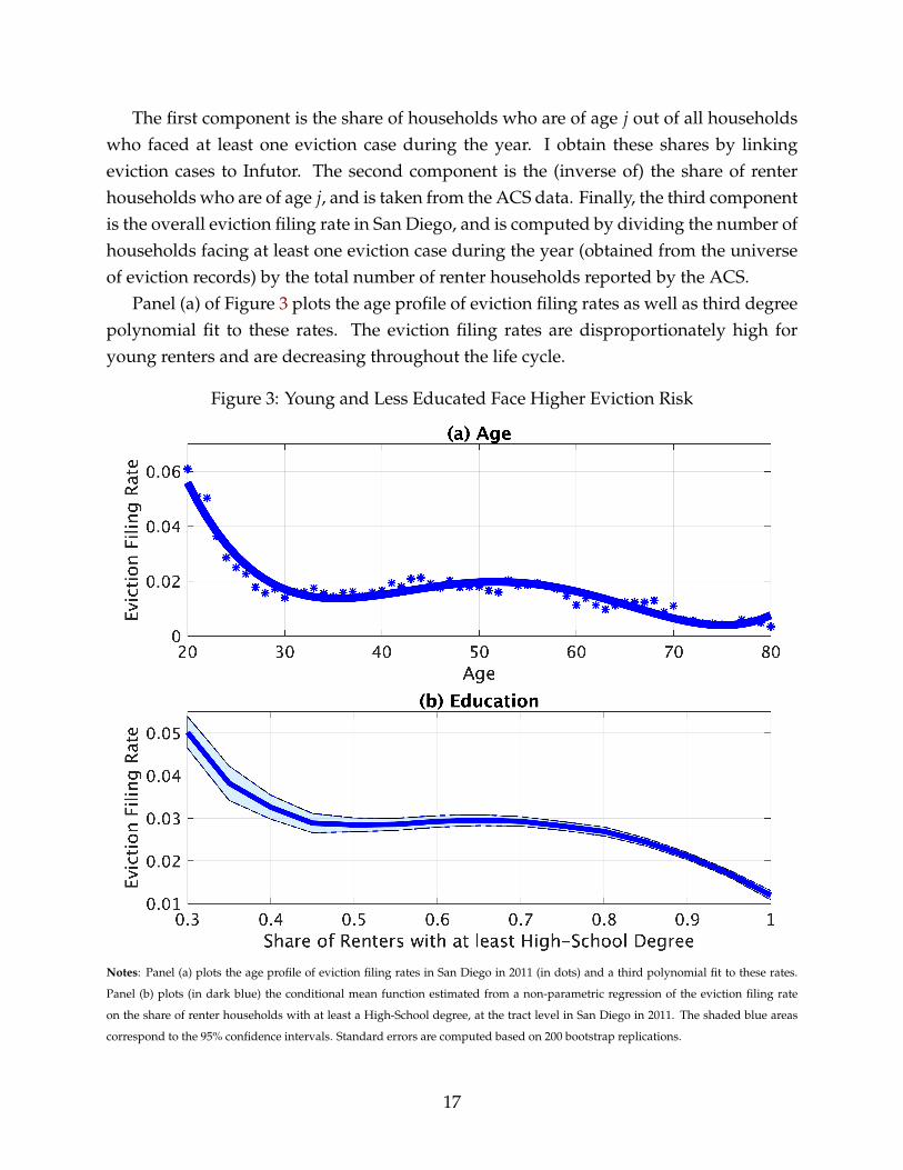
The first component is the share of households who are of age j out of all householdswho faced at least one eviction case during the year. I obtain these shares by linkingeviction cases to Infutor. The second component is the (inverse of) the share of renterhouseholds who are of age j, and is taken from the ACS data. Finally, the third componentis the overall eviction filing rate in San Diego, and is computed by dividing the number ofhouseholds facing at least one eviction case during the year (obtained from the universeof eviction records) by the total number of renter households reported by the ACS.

Panel (a) of Figure 3 plots the age profile of eviction filing rates as well as third degreepolynomial fit to these rates. The eviction filing rates are disproportionately high foryoung renters and are decreasing throughout the life cycle.

Figure 3: Young and Less Educated Face Higher Eviction Risk

Notes: Panel (a) plots the age profile of eviction filing rates in San Diego in 2011 (in dots) and a third polynomial fit to these rates.

Panel (b) plots (in dark blue) the conditional mean function estimated from a non-parametric regression of the eviction filing rate

on the share of renter households with at least a High-School degree, at the tract level in San Diego in 2011. The shaded blue areas

correspond to the 95% confidence intervals. Standard errors are computed based on 200 bootstrap replications.

17

Education and Eviction Risk. Since I do not observe the education attainment of defen-dants in the eviction data, I examine the relationship between eviction risk and educationat the tract level in San Diego. I compute the eviction filing rate for each tract by dividingthe number of households facing at least one eviction case in the tract by the number ofrenter households in the tract obtained from the ACS. As a measure of education, I cal-culate the share of renter households in the tract that have at least a High-School degreefrom the ACS data. I find that there is a strong and negative association between this mea-sure of education and eviction risk. This is shown in Panel (b) of Figure 3, which plots theconditional mean function estimated from a non-parametric regression of eviction filingrates on my measure of education.16

The Persistent Nature of Job-Loss and Divorce Risk. Panels (c) and (d) of Figure 2show that job-losses and divorces are associated with persistent income consequences.First, job-loss leads to a persistent unemployment state, as illustrated by the job-findingrates in Panel (d). In particular, for young and less educated households, who are atmost risk to lose their job and default on rent, unemployment spells typically persist forapproximately three months. Divorce has persistent consequences because individualswho divorce are more likely to lose their job and enter an unemployment spell. This isillustrated by Panel (c), which plots the job-loss rates for heads of households who weremarried in the previous month but are currently single. The high job-loss rates associatedwith divorce mostly reflects cases where a married household with only one breadwinnersplits, and the household formed by the spouse is left with no income.

Additional Facts. In Appendix C.1, I use PSID data to document additional facts onthe income dynamics associated with defaults. In particular, I show that the populationsthat are at most risk of default, namely the young and less educated, are also poorer.These populations, as well as individuals who have recently divorced, are not only morelikely to lose their job, but also draw their labor earnings from a more risky distribution.These facts, together with the facts documented in this section, guide the specificationand estimation of income risk faced by households in the quantitative model.

3.3 Rent Burden

A key question for studying housing insecurity is how much low-income householdsspend on rent. The common view in the macro-housing literature is that the share ofincome spent on rent — commonly defined as rent burden — is independent of renters’

16For robustness, I replicate the analysis with a different measure of human capital: the share of renterhouseholds in the tract that have a college degree (see Appendix Figure D.1).

18

income. This is guided by the observation that median rent burden is constant across USMSAs (Davis and Ortalo-Magné, 2011). I begin by verifying this regularity for later peri-ods, using the 2010-14 ACS data.17 Consistent with Davis and Ortalo-Magné (2011), anddespite substantial variation across cities in terms of median household income, I findthat the median rent burden is nearly constant at about 0.24, with a low standard devi-ation of 0.02 (Table D.2 in the Appendix provides more details). However, the data alsoreveals a wide variation across households: the standard deviation of rent burden acrosshouseholds within a particular MSA is on average 0.22 (fourth column of Table D.2). Thisobservation naturally raises the question whether in fact poor and rich households spendthe same share of their income on rent.

Figure 4: Rent Burden

Notes: Panel (a) plots (in dark blue) the conditional mean of rent burden given household income. The light blue areas correspond to

the 95% confidence intervals, computed based on 200 bootstrap replications.

17I exclude households living in group quarters, households reporting a rent burden that is larger than1.2, and households with annual income above $150, 000.

19

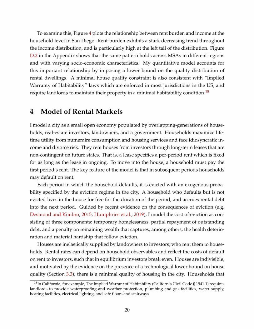
To examine this, Figure 4 plots the relationship between rent burden and income at thehousehold level in San Diego. Rent-burden exhibits a stark decreasing trend throughoutthe income distribution, and is particularly high at the left tail of the distribution. FigureD.2 in the Appendix shows that the same pattern holds across MSAs in different regionsand with varying socio-economic characteristics. My quantitative model accounts forthis important relationship by imposing a lower bound on the quality distribution ofrental dwellings. A minimal house quality constraint is also consistent with “ImpliedWarranty of Habitability” laws which are enforced in most jurisdictions in the US, andrequire landlords to maintain their property in a minimal habitability condition.18

4 Model of Rental Markets

I model a city as a small open economy populated by overlapping-generations of house-holds, real-estate investors, landowners, and a government. Households maximize life-time utility from numeraire consumption and housing services and face idiosyncratic in-come and divorce risk. They rent houses from investors through long-term leases that arenon-contingent on future states. That is, a lease specifies a per-period rent which is fixedfor as long as the lease in ongoing. To move into the house, a household must pay thefirst period’s rent. The key feature of the model is that in subsequent periods householdsmay default on rent.

Each period in which the household defaults, it is evicted with an exogenous proba-bility specified by the eviction regime in the city. A household who defaults but is notevicted lives in the house for free for the duration of the period, and accrues rental debtinto the next period. Guided by recent evidence on the consequences of eviction (e.g.Desmond and Kimbro, 2015; Humphries et al., 2019), I model the cost of eviction as con-sisting of three components: temporary homelessness, partial repayment of outstandingdebt, and a penalty on remaining wealth that captures, among others, the health deterio-ration and material hardship that follow eviction.

Houses are inelastically supplied by landowners to investors, who rent them to house-holds. Rental rates can depend on household observables and reflect the costs of defaulton rent to investors, such that in equilibrium investors break even. Houses are indivisible,and motivated by the evidence on the presence of a technological lower bound on housequality (Section 3.3), there is a minimal quality of housing in the city. Households that

18In California, for example, The Implied Warrant of Habitability (California Civil Code § 1941.1) requireslandlords to provide waterproofing and weather protection, plumbing and gas facilities, water supply,heating facilities, electrical lighting, and safe floors and stairways

20

cannot afford to move into the lowest quality house become homeless. The governmentlevies a lump-sum tax on investors to finance the externality costs of homelessness.

4.1 Households

Households live for A months. They derive a per-period utility U(ct, st) from numeraireconsumption ct and housing services st during lifetime, as well as a bequest utility νbeq(wt)

from the amount of wealth wt left in the period of death. They maximize expected lifetimeutility and discount the future with parameter β. Households consume housing servicesby renting houses of different qualities h from a finite set H. Occupying a house of qual-ity h at time t generates a service flow st = h. Households that do not occupy a houseare homeless. The service flow from homelessness is st = u and is assumed to be worsethan the services produced by the worst house (u < h, ∀h ∈ H). Households can save inrisk-free bonds with an exogenous interest rate r but are borrowing constrained. They areborn with an innate human capital e.

Marital Status. Each period households are either single (mt = 0) or married (mt = 1).Transitions between marital states happen with exogenous marriage and divorce prob-abilities, M(a, e) and D(a, e), which, consistent with the data, can depend on age andhuman capital. Let divt denote the divorce shock indicator that is equal to 1 if a house-hold divorced at time t and is equal to 0 otherwise. I assume single households marryspouses from outside the city, and that upon divorce one spouse leaves the city. This im-plies the number of households in the city doesn’t change with marriages and divorces.When a household marries its savings are doubled and when it divorces its savings arecut by half. As discussed below, income dynamics also depend on marital status and ondivorce events.

Income. Following the standard literature on idiosyncratic income processes (e.g. Abowdand Card 1989; Meghir and Pistaferri 2004; Heathcote, Perri and Violante 2010), house-hold income is composed of a deterministic age profile as well as persistent and transi-tory shocks. However, guided by the facts on the nature of risk that drives default on rent(Section 3.2), I make three modifications. First, I explicitly model an unemployment state.Second, I model divorce as a source of income risk by allowing the distribution of shocksto depend on divorce events. Finally, the deterministic component and the distributionof shocks are allowed to depend on age, human capital and marital status.

21

During their working life, households receive an idiosyncratic income given by

yt =

f (at, e, mt)ztut zt > 0

yunemp(at, e, mt) zt = 0. (1)

The first term f (at, e, mt) is the deterministic “life-cycle” component of income. Itis assumed to be a quadratic polynomial in age and its parameters can vary with hu-man capital and marital status. The second term zt is the persistent component of in-come and follows a Markov chain on the space z1, ..., zS with transition probabilitiesπz′/z(at, e, mt, divt) that depend on the household’s age, human capital, marital status,and on whether it was hit by a divorce shock. I assume z1 = 0 and interpret this realiza-tion of the persistent shock as unemployment. Similarly, ut is an i.i.d transitory incomecomponent drawn from a finite state space with probabilities πu(e, mt, divt). Unemployedhouseholds receive benefits yunemp(at, e, mt) that depend on age, human capital and mar-ital status. Households retire at age a = Ret, after which they receive a deterministicincome yRet(e, mt).

4.2 Rental Leases and Evictions

Households rent houses from real-estate investors via long-term, non-contingent, leases.That is, a lease specifies a per-period rent that is fixed for the entire duration of the lease.The rent on a lease that begins at time t on a house of quality h is given by qh

t (at, yt, wt).It can depend on the age, the income, and the total wealth of the household at the periodin which the lease begins, but is non-contingent on future realizations. To move into thehouse, households must pay the first period’s rent. However, in subsequent periods, theyhave the ability to default on rent.

When a household begins to default, an eviction case is filed against it. The evictioncase proceeds until the household is evicted or until it stops defaulting. Each period inwhich the household defaults, including the first period of the default spell, it is instan-taneously evicted with probability p. The benefit of default is that if the household is notevicted, it consumes the housing services for the duration of the period without payingrent. Rental debt then accrues with interest r to the next period. Households with out-standing debt from previous periods can either repay the debt they owe, in addition to theper-period rent, or can continue to default and face a new draw of the eviction realization.

The costs of default are the consequences of potential eviction. Evicted tenants becomehomeless for the duration of the period, and pay the investor a share φ of any outstand-

22

ing rental debt they have accumulated from previous periods.19 Eviction also imposes adeadweight loss in the form of a proportional penalty λ on any remaining wealth.

The lease terminates when the household is evicted. Leases also terminate throughone of the following channels. First, households that occupy a house are hit by an i.i.d.moving shock with probability σ every period. Second, houses are hit by an i.i.d. de-preciation shock with probability δ, in which case the house fully depreciates and thehousehold moves. Finally, leases end when the household dies.20

4.3 Household Problem

Households begin each period in one of two occupancy states Ot: they either occupy ahouse (Ot = occ) or not (Ot = out). In what follows, I describe the problems faced by anon-occupier and occupier household. Bellman equations are given in Appendix B.1.

Non-occupiers. The state of a household that begins period t without a house is summa-rized by xout

t = at, yt, zt, wt, mt, e. Given the rental rates, the household decides whetherto move into a house h ∈ H or to become homeless. If the household moves into a houseof quality h, it must pay the rent qh

t (at, yt, wt). It consumes the service flow provided bythe house (st = h), and divides remaining wealth between consumption and savings.It then begins the next period as an occupier (Ot+1 = occ), unless a moving shock ora house depreciation shock are realized between t and t + 1. If instead the householdbecomes homeless, for example because it cannot afford the first period’s rent, then itshousing service flow is st = u. Homeless households also make a consumption-savingchoice, and begin the next period as non-occupiers.

Occupiers. The state of a household that begins period t under an ongoing lease (Ot =

occ) is summarized by xocct = at, zt, wt, mt, e, ht, qt, kt, where ht is the quality of the house

that it occupies, qt is the per-period (pre-determined) rent on the ongoing lease, and kt isthe outstanding rental debt the household might have accumulated from previous de-faults. Taking the eviction regime as given, the occupier household decides whether todefault or not. To avoid default, the household must pay the per-period rent, but alsoany outstanding rental debt. In case of default, the eviction draw is immediately realized.Households that begin the period as occupiers also choose how to divide any wealth thatis not spent on housing between consumption and savings.

19Households with wealth that is lower than this amount of debt repay their entire wealth. In practice,in the numerical solution I assume that when households repay their entire wealth, the are endowed witha small, predetermined, ε > 0 of dollars.

20Households with positive outstanding debt, who move due to a moving shock or a depreciation shock,or who die, are required to pay a fraction φ of their debt (or their entire wealth, if wealth is insufficient).

23

4.4 Real-Estate Investors

Real-estate investors have access to the housing market, in which they can buy houses ofqualities h ∈ H from landowners. The house price of a house of quality h is given by Qh

t .Investors can buy as many houses as needed and rent them to households. In addition tothe cost of buying a house, investors incur a per-period cost τh (proportional to the housequality) for as long as the rental lease is ongoing. Importantly, this cost is paid regardlessof whether or not the tenant pays the rent or defaults, which implies that default is costlyfor investors. When the lease terminates, investors immediately resell the house (unlessthe termination is due to a depreciation shock, in which case the house is worth nothing).Investors discount the future at rate (1 + r)−1.

Investors observe the household’s age, income and wealth at the period in which thelease begins. They are assumed to price the per-period rent (which is then fixed for theduration of the lease) in a risk-neutral manner, such that for each lease they break evenin terms of expected profits. The zero profit condition is given in Appendix B.2. It isuseful to decompose the rent into a risk-free rent component, which is defined as the rentcharged from households with zero default risk, and a default premia component, whichis the difference between the rent charged and the risk-free rent.

An example for this decomposition is given in Appendix B.3. The risk-free rent is anincreasing function of the house price, since investors assume these costs regardless of thehousehold’s default behavior. The default premia is increasing with the tenant’s defaultrisk, since default is costly for investors: delinquent tenants repay only a fraction of theiraccumulated debt when they are evicted. The default premia is also higher when it isharder and more costly to evict delinquent tenants, i.e. when the likelihood of evictiongiven default p, and the share of debt repaid upon eviction φ, are lower.21

4.5 Landowners

There is a representative landowner for each house quality h ∈ H. The landowner oper-ates in a perfectly competitive housing market and solves a static problem each period. Itobserves the house price Qh

t and chooses the amount Xht of houses to supply given a de-

creasing returns to scale production technology. The cost to construct Xht houses in terms

of numeraire consumption is:21In theory, the effect of p on rents is ambiguous. On the one hand, a lower likelihood of eviction given

default implies that tenants can stay for longer in the house without paying rent, which is costly for in-vestors and therefore raises equilibrium rents. On the other hand, a longer eviction process means thatdelinquent tenants have a better chance to repay their debt to the investor. In practice, the former dom-inates in the quantitative application since the risk that drives defaults is persistent in nature, such thatdelinquent tenants are unlikely to repay their debt even when the process is prolonged.

24

C(Xht ) =

1ψh

0

(Xh

t)(ψh

1)−1

+1(ψh

1

)−1+ 1

.

The problem of the firm reads as:

maxXt

Qht Xh

t −1

ψh0

(Xh

t)(ψh

1)−1

+1(ψh

1

)−1+ 1

.

The per-period supply of new houses of quality h is therefore:

(Xh

t

)∗=(

ψh0 Qh

t

)ψh1 , (2)

where ψh0 ≥ 0 is the scale parameter, and ψh

1 > −1 is the elasticity of supply with respectto house price.

4.6 Government

The role of the local government is to finance two types of costs. The first is the costof homelessness to the city, which is assumed to be a linear function of the size of thehomeless population. In particular, the per-household cost of homelessness is θhomeless.Second, the government finances the monetary costs of rental market policies that arelater considered in the counterfactual analysis, for example of providing legal counsel tohouseholds facing eviction cases or of subsidizing rent. For now, I parsimoniously denotethese costs by Λ and discuss them in detail in Section 6. The government finances its costsby levying a lump-sum tax Tax on investors, who are assumed to be deep pocketed. Thegovernment’s budget therefore satisfies:

θhomeless

∫i

1st=udi + Λ = Tax. (3)

4.7 Stationary Recursive Equilibrium

The economy’s eviction regime is summarized by the pair (p, φ). A stationary recursiveequilibrium is defined as a set of household policies, landowners policies, rents qh(a, y, w),house prices Qh, and a distribution Θ∗ of household states, such that:

a) Households’ and landowners’ policies are optimal given prices.

b) Investor break even in expectation given prices and household optimal behavior.

25

c) The housing market clears for every segment h ∈ H.

d) The distribution Θ∗ is stationary.

A Stationary Distribution. The idiosyncratic state of a household at time t is summa-rized by ωt = (Ot, at, zt, wt, mt, e, ht, qt, kt). I denote the state space by Ω and the period tdistribution of agents over Ω by Θt such that Θt(ω) is the share of the population at stateω at time t. The transition function T (ω, ω′) is the probability that a household with acurrent state ω transits into the state ω′. It is based on exogenous shocks and endogenoushousehold policies. The share of population in state ω′ in period t + 1 is therefore:

Θt+1(ω′) =

∫T((ω, ω′

)dΘt(ω).

A stationary distribution Θ∗ is a fixed point of this functional equation.

4.8 Rental Market Policies Through the Lens of the Model

Insurance. A common goal of policies that address evictions and homelessness is to pro-vide insurance to tenants who cannot pay rent. One way this can be done is by makingit harder to evict delinquent tenants, for example by providing legal counsel in evictioncases. In the model, this implies a lower likelihood of eviction given default, p. Means-tested rental assistance, which in the model are financed by the local government, is an-other popular proposal to insure low-income tenants.

Households value insurance in the presence of otherwise non-contingent rental leases.Contingency helps households smooth their consumption across states and avoid thecost of homelessness and eviction in bad times. Importantly, the presence of a minimalhouse quality means that contingency is valuable even when households are risk neutraland when there is no eviction penalty. A minimal house quality constraint implies thathouseholds cannot always downsize to lower quality houses in bad times, and greaterinsurance can therefore protect them homelessness. This feature distinguishes the modelfrom the standard models of default on consumer debt (Livshits, MacGee and Tertilt,2007; Chatterjee et al., 2007) and sovereign debt (Eaton and Gersovitz, 1981; Aguiar andGopinath, 2006; Arellano, 2008), in which households can always downsize consumption.

Rents and housing supply. At the same time, rental market policies also affect rentsand housing supply in equilibrium. Consider first a policy that makes it harder to evictdelinquent tenants. In equilibrium, investors are compensated by higher default premia,which can in turn push low-income households into homelessness if they can no longer

26

afford to move into the minimal level of housing. Among households who can still rent,some are forced to downsize in response to the higher default premia, driving a shiftin demand for housing from upper to lower housing quality segments. In equilibrium,housing supply adjusts, and because supply is not perfectly elastic house prices are alsoaffected. Changes in house prices translate to changes in risk-free rents, which are a com-ponent of rents paid by all renters, including those with zero default risk. Thus, policiesthat change the eviction regime can affect the entire renter distribution through their ef-fect on housing supply. The inelastic housing supply assumption contrasts my modelwith models of default on debt, in which credit supply is assumed to be perfectly elas-tic, and policies that change the leniency of default laws affect only agents who have anon-zero default risk.

Means-tested rental assistance programs have conceptually different implications. In-stead of making it harder to evict tenants who have already defaulted, rental assistancelowers the likelihood that tenants default. In equilibrium, this implies that the default pre-mia charged by investors are lower. As more households can afford to sign rental leases,demand for housing rises. In equilibrium, housing supply adjusts through changes tohouse prices, and risk-free rents are again affected.

Local rental market characteristics. Quantitatively, the effect of policies depends onlocal rental market characteristics. First, when default on rent is driven by persistentshocks to income, policies that make it harder to evict delinquent tenants are less effectivein preventing evictions and homelessness. When risk is persistent in nature, tenants whodefault are unlikely to bounce back and repay their debt even if they have longer periodsof time to do so, and are likely to end up being evicted and becoming homeless despitethe stronger protections. Second, the elasticity of housing supply in the city governs howpolicies affect housing supply and the risk-free component of rent. For example, whenhousing is less elastic, e.g. due to land use regulations, policies that induce a rise indemand lead to larger increases in the risk-free rent.

5 Quantification and Model Fit

I quantify the model to San Diego County, California, for reasons previously discussed inSection 3. The time period is monthly. It is helpful to group the model inputs into fourcategories: (1) the income process, (2) the eviction regime, (3) parameters estimated in-dependently based on direct empirical evidence or existing literature, and (4) parametersestimated internally to match micro data on rents, evictions and homelessness.

27

5.1 Income

For the transitions between employment (zt > 0) and unemployment (zt = 0), I as-sume job-loss and job-finding probabilities JL(at, e, mt, divt) and JF(at, e, mt, divt), whichdepend on age, human capital, marital status and divorce events. I assume that whenpositive, zt follows an AR1 process in logs with an autocorrelation and variance that de-pend on human capital, marital status and divorce shocks:

log zt = ρ(e, mt, divt)× log zt−1 + εt, (4)

εt ∼ N(

0, σ2ε (e, mt, divt)

).

Finally, the transitory component ut is assumed to be log-normally distributed withmean zero and variance σ2

u(e, mt, divt) that depends on human capital, marital status anddivorces. When finding a job, households draw z and u from their invariant distribution.

The specification of the income process is designed to capture the empirical facts onthe risk that leads tenants to default, as documented in Section 3.2. First, It accountsfor job-loss risk by explicitly modeling an unemployment state. Second, it accounts fordivorce risk, namely the fact that divorce is associated with a higher job-loss rate, byallowing job-loss rates to depend on divorce events. Finally, in order to capture the factthat young and less educated households are more likely to lose their job and to divorce,job-loss and divorce rates are age and human capital dependent.

The specification is also guided by additional facts on the income dynamics associatedwith defaults, which are documented in Appendix C.1. First, the deterministic compo-nent of income depends on age, human capital and marital status to account for the factthat young, less educated and single households are poorer on average. The parametersof the AR1 process and of the transitory shock depend on human capital, marital statusand divorce events to account for the fact that less educated, single, and especially indi-viduals who recently divorced, draw their labor earnings from a more risky distribution.

The estimation of the parameters of the income process targets and matches the em-pirical facts described above. The estimation is discussed in detail in Appendix C.2.

5.2 Eviction Regime

In the model, the expected length of an eviction case, from initial default to eviction, is 1/pmonths. The likelihood of eviction given default, p, is therefore identified by the (inverseof the) average number of months that evicted tenants in San Diego stay in their housebetween default and eviction. The garnishment parameter φ is identified by the share of

28

rental debt that evicted tenants in San Diego repay their landlords. To quantify these twomoments, I use the findings of the The Sargent Shriver Civil Counsel Act (AB590).

Funded by the Judicial Council of California between 2011 and 2015, the Shriver Actestablished pilot projects to provide free legal representation for individuals in civil mat-ters such as eviction cases, child custody, and domestic violence. I focus on the pilotproject that provided legal counsel in eviction cases in San Diego County. For each case,the Shriver Act staff recorded information on key case outcomes, namely whether thetenant was evicted, the length of the eviction case from filing to resolution, and the shareof rental debt evicted tenants were ordered to repay their landlords. The mean outcomesfor tenants represented by Shriver lawyers are reported in an evaluation report writtenby the Shriver Act Implementation Committee (Judicial Council of California, 2017).

The Shriver team also conducted an RCT across the counties of San Diego, Los An-geles and Kern, in which tenants facing eviction cases were randomly assigned to re-ceive legal counsel.22 The reported differences in mean outcomes between representedand non-represented tenants across the three counties, together with the mean outcomesreported for represented tenants in San Diego, allow imputing the mean outcomes fornon-represented tenants in San Diego.

In particular, represented tenants in San Diego who were evicted stayed in their housefor an average of 50 days between default and eviction, and were ordered to repay 56.5%of their rental debt.23 The RCT reports that non-represented tenants who were evictedremained in their house for an average of 12 days less between default and eviction, andpaid 15% more of their debt.24 Thus, I impute that non-represented tenants in San Diegowho were evicted stayed in their house for an average of 38 days between default andeviction, and were ordered to repay an average of 71.5% of their rental debt.

In the baseline quantification, I make the assumption that tenants facing eviction cases

22Random assignment protocols were conducted, for 1 month. Low-income tenants who presented forassistance with an unlawful detainer case and who were facing an opposing party with legal representationwere randomly assigned to either (a) receive full representation by a Shriver attorney, or (b) receive noShriver services. Across these three pilot projects, a total of 424 litigants were assigned. Findings arereported after aggregating across the three pilot projects.

23Table H25 of the evaluation report (Judicial Council of California, 2017) states that the mean numberof days to move for tenants who had to move out as part of the case resolution was 47, from case filing tomove-out. I add the 3 day required notice period that a landlord has to give the tenant before filing a casein California. Table H25 also reports that 30% of evicted tenants were ordered to pay their rental debt infull, 26% paid a reduced amount, and rental debt was waived for 20% (for the remaining 24% the amountwas unknown). Under the assumption that for cases classified as “reduced payments” the share paid bythe tenant is 50%, the mean share of repaid debt is (0.3× 1 + 0.26× 0.5)/0.76 = 0.565.

24Table H54 of (Judicial Council of California, 2017) reports the differences between control and treat-ment in terms of time to move out. Table H57 reports the differences in terms of amounts awarded relativeto amounts demanded by landlords. I assume 100% of demanded amount was rewarded when “full pay-ment” or “additional payment” were maid, and 50% was rewarded in cases with “reduced payments”.

29

in San Diego do not have legal counsel. This assumption, which is motivated by extensiveevidence showing that legal counsel in eviction cases is extremely rare,25 allows me toidentify the eviction regime parameters p and φ from the moments I imputed for the non-represented tenants. Namely, I set p =

(3038

)−1= 0.7895 and φ = 0.715. As discussed

in Section 6.1, I later use the moments reported for represented tenants to identify theeviction regime associated with a “Right-to-Counsel” counterfactual, where all tenantsare represented by lawyers.

5.3 Independently Estimated Parameters

When possible, remaining parameters are estimated independently based on direct em-pirical evidence or existing literature.

Technology. Households enter the economy at age 20 and die at age 80. Using data fromthe Survey of Income and Program Participation, Mateyka and Marlay (2011) find that themedian tenure of renters is 2.2 years (or 27 months). As such I set the moving shock toσ = 0.037. The per-period cost parameter τ is estimated to capture a 1.25 percent annualproperty tax in California. The depreciation rate δ is estimated to capture a 1.48 percentannual depreciation rate, based on evidence from the Bureau of Economic Analysis (as inJeske, Krueger and Mitman, 2013). I set the monthly interest rate r to be consistent withan annual interest rate of 1 percent. The elasticities of housing supply ψh

1 are set to 0.67based on Saiz (2010), who estimates supply elasticities at the metro area level. I assumehousing supply elasticities are equal across all house segments h ∈ H within the city.

Cost of Homelessness. To estimate the per-household cost of homelessness θ, I proceedin two steps. First, I use the San Diego Taxpayers Educational Foundation’s (SDTEF)report, which estimates that the total annual cost of homelessness in San Diego in 2015 is200 million dollars.26 This includes, for example, the costs of shelters and other temporaryhousing, the financing of food banks, mental and physical health costs, policing costs,and of the costs of homelessness prevention activities.27 Second, I estimate the size of thehomeless population in San Diego in 2015, combining data from the 2015 ACS and the

25For example, in San Diego, less than 5 percent of tenants facing eviction cases have legal counsel ofthe evaluation report (Judicial Council of California, 2017) states. Humphries et al. (2019) report similarnumbers in Cook County, IL.

26https://www.sdcta.org/studies-feed/2019/3/22/homelessness-expenditure-study27Estimating the costs of homelessness to local governments is a complicated task. To validate the SDTEF

estimates, I refer to an additional study conducted in Orange county, which boarders with San Diego andhas a similar sized population (https://www.jamboreehousing.com/pages/what-we-do-resident-services-permanent-supportive-housing-cost-of-homelessness-study). This study estimates the cost to tax-payers tobe similar to that in San Diego.

30

2015 Point-in-Time Count.Using the ACS, I classify a family as homeless if it falls into one of two categories. First,

if I can identify it as “sheltered homeless”, i.e. living in a homeless shelter.28 Second, Ialso count families as homeless if they “double up”, i.e. live in the house of anotherhousehold, and are so poor they are unlikely to be able to rent a house by themselves.29

The ACS does not record information about “unsheltered homeless”, i.e. families liv-ing on the streets. To account for those, I use the Point-in-Time count published by theHUD, which provides a city-level estimate of the number of sheltered and unshelteredhomeless individuals in a given evening in January, at an annual frequency.30 I then in-flate the number of “sheltered homeless” families from the ACS to account for the relativesize of sheltered versus unsheltered individuals in the Point-in-Time count.

My definition of homelessness is broader than the HUD’s definition of “literally home-less”, which includes only sheltered and unsheltered homeless, and is consistent withthe Department of Education’s definition, which also includes “doubled up” families(see Meyer et al., 2021 for a review). According to this definition, 3.29% of the house-holds in San Diego, or 37, 000 households, were homeless in 2015. Thus, the averageper-household monthly cost of homelessness is estimated as $450.2.

Preferences. Felicity is given by CRRA utility over a Cobb-Douglas aggregator of nu-meraire consumption c and housing services s:

U(c, s) =[c1−ρsρ

]1−γ

1− γ.

Guided by evidence on rent-burden in San Diego (ACS, 2015), the weight on housingservices consumption ρ is set to 0.3.31 The parameter γ governs both the relative riskaversion and the inter-temporal elasticity of substitution. I set γ = 1.5, as in Gourinchas

28Homeless shelters are one of many categories of living arrangements that the Census bundles togetheras “group quarters”. I rule out many alternative categories by keeping only non-institutionalized adultswho are non-student, non-military, and who’s annual income is less than 20, 000$. An annual incomebelow this threshold implies that the family would have to spend at least 50% of its income to afford theaverage rent in the bottom quartile of the rent distribution in San Diego, which is considered as “heavilyrent-burdened” by the HUD.

29I classify a sub-family as “doubled up” if it is classified by the Census as a “sub-family” and its annualincome is less than 20, 000$. The Census defines a family as a sub-family living in another household’shouse if the reference person of the sub-family is not the head of the household and the family is either acouple (with or without children), or a single parent with children. This definition means I do not includesingle roommates without dependents who double-up (including roommates) in my homeless count.

30https://www.sandiego.gov/sites/default/files/newsrelease150423.pdf.31Under perfectly divisible housing and without the ability to save, ρ = 0.3 implies all households would

choose a rent-burden of 30%, matching the median in the data. In practice, median rent burden in the modelends up being slightly higher due to the minimal house size constraint.

31

and Parker (2002). The functional form of bequest motives is taken from De Nardi (2004):

νb(w) = κw1−γ

1− γ,

where the term κ reflects the household’s value from leaving bequests. I set κ = 0.5 basedon Landvoigt, Piazzesi and Schneider (2015).

5.4 SMM Estimation

The parameters I do not have direct evidence on are: (1) the set of house qualities H, (2)the eviction penalty λ, (3) the housing supply scale ψh

0 for every h ∈ H, (4) the home-lessness (dis)utility u, and (5) the discount factor β. I consider a model with three housequalitiesH = h1, h2, h3 and estimate the nine parameters jointly to match nine data mo-ments. The parameters are estimated by minimizing the distance between model anddata moments using a Simulated Method of Moments (SMM) approach. Table 1 summa-rizes the jointly estimated parameters and data moments. Parameters are linked to thedata targets they affect most quantitatively.

Table 1: Internally Estimated Parameters

Parameter Value Target Moment Data Model

TechnologyHouse qualities (h1, h2, h3) (600, 000,

775, 000,1, 070, 000)

Average rent in 1stquartile, 2nd quartile, tophalf

($800;$1, 200;$1, 800)

($800;$1, 200;$1, 800)

Supply scales(ψ1

0, ψ20, ψ3

0)

(127, 6.35,5.99) ×10−6

Average house price in 1stquartile, 2nd quartile, tophalf

($235, 000;$430, 000;$700, 000)

($235, 000;$430, 000;$700, 000)

Eviction penalty λ 0.975 Eviction filing rate 2.0% 2.0%

PreferencesHomelessness utility u 75, 000 Homelessness rate 3.29% 3.29%Discount factor β 0.971 Median wealth - renters $5, 000 5, 500$

House qualities. I estimate h1, the house quality in the bottom segment, so that theaverage rent in this segment matches the average rent in the bottom quartile of rents inSan Diego, computed from the 2015 ACS data (and illustrated by the green vertical linein Figure D.3, which plots the distribution of rents in San Diego). Similarly, I estimate h2

32

and h3 so that the average rent in the middle and top segments match the average rentin the second quartile and the average rent in the top half of the rental rate distributionin San Diego. Since on average, default premia are negligible, the average rent in eachsegment in the model is approximately equal to the risk-free rent in that segment, whichis in turn a function of the per-period cost τh and of the house price in that segment (seeAppendix B.3). Given the observed house price in the segment, the house quality h thenadjusts to ensure that the average rent matches the data.32

The minimum house quality h1 is of particular importance. Households that cannotafford to sign a lease on this house cannot downsize any further and therefore becomehomeless. I pick the average rent in the bottom quartile, which is $800, as my data target,since renting a house for less than $800 in San Diego does not seem to be a feasible option.In fact, less than 5% of renters in the ACS report a rent below this threshold.

Supply scales. The scale parameters of housing supply(ψ1

0, ψ20, ψ3

0)

are set to matchhouse prices in the data. For consistency with the rent data moments, I target the averagehouse price in the bottom quartile, second quartile and top half of the 2015 ACS houseprice distribution in San Diego. Rents and the income distribution determine the demandfor houses in each segment in the model. The scale parameter has to be such that theoptimal quantity supplied given the observed house prices is equal to the demand. It issubstantially lower in the middle and top segments because demand in these segments islower relative to the observed house price.

Eviction penalty. The eviction penalty λ is estimated to 0.975.33 Intuitively, it is mostlyidentified by the eviction filing rate in the data. When the penalty is lower, eviction is lesscostly and more households default on rent. The eviction filing rate in the model, whichis the share of renter households who defaulted on rent at least once in the past year (andtherefore faced an eviction filing), is then higher. The eviction filing rate in the data ismeasured using the universe of eviction court cases in San Diego (Section 3.2).

Homelessness (dis)utility. The disutility from homelessness u is mostly identified bythe homelessness rate in San Diego, which is estimated to be 3.29% (see Section 5.3).34

When u is lower, homelessness is less costly and more households choose not to sign

32The estimation suggests that, as opposed to models with free conversion of houses, rents are not alinear function of house quality model. In particular the rent per quality unit is higher in the middle andtop segments. Because houses in the middle and top segments are much more expensive than in the middlesegments, but the differences in rents are less pronounced, the rent per quality unit in these segments ishigher. This crowds the bottom segment and works to increase house prices there.

33Although λ is relatively large, the penalty in terms of dollars is usually low because households thatare evicted typically have low income and no savings.

34The estimation implies that a household living in the minimal house size would require a 140% increasein its consumption in order to agree to become homeless for the duration of the period.

33

rental leases. It is useful to note that the homelessness disutility and the eviction penaltyare separately identified. This is because the homelessness disutility affects both thosewho are not able to move into a house and those who are evicted, but the eviction penaltyaffects only those who are evicted.

In particular, a lower u leads to a drop in both homelessness and eviction filings, ashomelessness and eviction (and hence default) become more costly. The eviction penaltyλ moves the two moments in opposite directions. A higher eviction penalty makes defaultless attractive, hence lowering the eviction filing rate, but actually makes homelessnessmore attractive, thereby increasing the homelessness rate. This is because staying outof the rental market eliminates the risk of eviction, which has become more punitive.Put differently, the eviction penalty and the homelessness disutility allow the model tomatch both the eviction filing rate and the homelessness rate, which are both importantmoments for studying housing insecurity.

Discount factor. I set the discount factor β to 0.971 to match the median wealth ofrenters in urban areas in California. Computed from the PSID as the “wealth” variable,which is the sum of all assets minus all types of debt, renters’ median wealth is 5, 000$.35

5.5 Model Fit to Non-Targeted Moments

As a check of the model’s quantification, I evaluate its fit to non-targeted moments in thedata. In particular, I show that the model performs well in matching the characteristicsof households who face eviction cases, as well as the empirical relationship between rentburden and household income.

The Cross-Section of Eviction Filing Rates. Figure 5 plots a third degree polynomial fitto the age profile of eviction filing rates in the model (in green) and data (in blue, repli-cating Panel (a) of Figure 3). The model accounts for the disproportionately high evictionfiling rates observed for very young households as well as for the general downwardtrend across ages. In the model, young households are more likely to default on rent(and face an eviction case) because they are poorer and more exposed to negative incomeshocks in the form of job loss and divorce (see Figure 2). The model under-predicts theeviction filing rate for the very old because after retirement households in the model faceonly modest divorce risk.

35This number is consistent with other data such as the Survey of Consumer Finances (SCF).

34

Figure 5: Age Profile of Eviction Filing Rates: Model and Data

Notes: Eviction filing rates in the data are taken from Figure 3. The eviction filing rate in the model is the share of renter households

who defaulted on rent at least once during the year.

The model also matches the share of eviction filings that are related to divorces. Asshown in Figure 1, 21.3 percent of evictions are due to a divorce. In the model, 20 percentof eviction filings happen when a divorce shock hits. Divorce can lead to default in themodel because, as in the data, it is associated with income risk.

Rent Burden and Income. The empirical relationship between rent burden and house-hold income, documented in Section 3.3, is particularly important for studying housinginsecurity. Figure 6 shows that the model closely matches this relationship. As in the data(in blue), rent burden in the model (in green) is decreasing with household income andis particularly high for households at the left tail of the income distribution. The modelis able to generate this pattern because the minimal house quality constraint implies thatpoor households are limited in their ability to downsize their housing consumption. Thisis in contrast to the standard model of housing choice (e.g. Davis and Ortalo-Magné,

35

2011), which predicts a constant expenditure share on rent (Section 3.3).

Figure 6: Rent Burden and Household Income: Model and Data

Notes: The dark blue line plots the conditional mean function estimated from a non-parametric regression of rent burden on household

income, using 2010-14 5-year ACS. The shaded blue areas correspond to the 95% confidence intervals. Standard errors are computed

based on 200 bootstrap replications. The green line and shaded green areas are similarly computed from model simulated data.

5.6 The Role of Persistent and Transitory Shocks

As discussed in Section 4.8, the effects of policies that make it harder to evict delinquenttenants crucially depend on the nature of risk that drives defaults. In this section, I use thequantified model to show that the vast majority of default spells are driven by persistentincome shocks. To do so, I define the driver of default as the type of negative income shockthat hit the household at the initial period of the default spell. I then divide all defaultspells (or equivalently, eviction filings) in the steady state by their driver of default.

36

Figure 7: Drivers of Default

Notes: The default driver is the type of negative income shock that hit the household at the first period of a default spell. “Persistent”

(“Transitory”) corresponds to a persistent (transitory) income shock alone. “Persistent+Transitory” corresponds to a combination of

persistent and transitory shocks. The light (dark) blue parts correspond to shocks that are (aren’t) associated with divorce event.

Figure 7 shows that 68 percent of default spells are initiated by a negative persistentincome shock alone. I further separate those by whether a divorce shock hit at the sametime (in light blue) or not (in dark blue). 30 percent of default spells are initiated bya combination of both a persistent and a transitory negative shock, and only 2 percentof default spells begin with a purely transitory shock. This result is consistent with theempirical facts documented in Section 3, showing that defaults are driven by job-lossesand divorces, which are both associated with persistent income consequences.

Intuitively, households are more likely to default on rent when they are hit by a per-sistent shock, all else equal. Holding wealth fixed, poor households who are in a badpersistent state anticipate being poor in the future. Since future default is more likelyin this case, these households have lower incentives to pay the rent today. Figure D.4illustrates this by plotting the default policy function for households who differ in theirpersistent income states. In this environment, policies that make it harder to evict delin-

37

quent tenants might be limited in their ability to prevent evictions. When default is drivenby persistent shocks, delinquent tenants are unlikely to bounce back and repay their debt,even if they have longer periods of time to do so.

6 Counterfactuals

In this section, I use the quantified model to conduct three policy experiments. First,I evaluate the effects of a city-wide “Right-to-Counsel” legislation, which provides tax-funded legal representation to all tenants facing eviction cases. Second, I consider ameans-tested rental assistance program. Third, I evaluate a temporary moratorium onevictions following an unexpected unemployment shock of the magnitude that was ob-served in the US at the onset of COVID-19.

I evaluate these policies based on two complementary criteria. First, I consider howpolicies affect households’ welfare. Second, I evaluate the monetary costs that policiesimpose on the local government. Given that homelessness is costly for the government,policies that increase (decrease) the homelessness rate imply higher (lower) monetarycosts. In addition, the government also takes on the financing costs of the policy, forexample of providing legal counsel or rental assistance.

6.1 Right-to-Counsel

While “Right-to-Counsel” legislation has increasingly gained ground in recent years, itsequilibrium effects at the city level, when rents and housing supply can adjust, are stilllargely unknown (see Section 2.2 for a discussion). To evaluate these effects, I exploitmicro level evidence on how legal counsel changes the eviction regime parameters ofthe model, and compute a new steady state equilibrium under the counterfactual regimewhere all tenants facing eviction cases are provided with legal counsel.

The Shriver Act (see discussion in Section 5.2) finds that, on average, tenants with legalcounsel stay in their house for 50 days from the day they miss rent to the day they areevicted, compared to only 38 days for non-represented tenants. Represented tenants alsopay a lower share of rental debt when they are evicted: 56.5 percent versus 71.5 percentfor non-represented tenants. Thus, while the eviction regime parameters in the baselineeconomy (without legal counsel) are identified from the moments of the control group(p = 30

38 and φ = 0.45), the parameters associated with a city-wide “Right-to-Counsel”,where all tenants facing eviction cases are provided with legal counsel, are identifiedfrom the treatment group moments. I denote them by pRC = 30

50 and φRC = 0.3. Next, I

38

compute a new steady state equilibrium under the eviction regime (pRC, φRC), in which itis harder and more costly to evict delinquent tenants.

Rents, homelessness, and evictions. The main result is that “Right-to-Counsel” in-creases homelessness by 15 percent. The increase in default premia induced by the policypushes low-income households into homelessness, as they can no longer afford to moveinto the minimal level of housing. To illustrate the effect on rents, the right panel of Figure8 plots the CDF of rents in the bottom housing segment, before and after the reform. Rel-ative to the baseline economy (in green), the rent distribution under “Right-to-Counsel”(in blue) shifts to the right. In the baseline economy, default is not particularly costly forinvestors since renters who default are quickly evicted, and default premia are thereforerelatively low. Under “Right-to-Counsel”, default premia are higher, as it becomes harderand more costly to evict delinquent tenants.

Figure 8: Effects of Right-to-Counsel

Notes: The CDF of rents is computed based on observed rents in the bottom segment (and does not account for the shadow prices for

homeless households that are not renting). The eviction filing rate (eviction rate) is the share of renter households that defaulted on

rent (were evicted) during the past 12 months. The homelessness rate is the share of homeless households.

39

As a result, the homelessness rate increases by approximately 15 percent, from 3.29percent of the population in the baseline economy to 3.76 percent (see bottom bars in theleft panel of Figure 8). The eviction filing rate (upper bars) decreases from 2 percent to 1.7percent. However, the reason that relatively less renters default and face an eviction filingis that low-income tenants, who are the ones most at risk of default, are priced out of therental market and cannot rent in the first place. That is, when default costs are higher forinvestors, rents adjust such that the pool of households that are able to rent is less risky inequilibrium. These results highlight that the evaluation of policies that address evictionmust take into account their equilibrium effects on rents and homelessness.

The eviction rate (middle bars), which is defined as the share of renter householdswho were evicted at least once during the year (and is lower than the eviction filing ratebecause not all eviction cases are resolved in an eviction), also decreases from 1.9 percentto 1.5 percent. Similarly to the eviction filing rate, this drop is mostly explained by thefact that the renter population under “Right-to-Counsel” is less likely to default on rent.In theory, it can also be driven by the fact that given default, delinquent tenants are lesslikely to be evicted since they have longer periods of time to repay their debt. In whatfollows I show that this channel is quantitatively negligible.

To examine whether “Right-to-Counsel” is indeed able to prevent evictions of delin-quent tenants, I define the eviction-to-default rate. The eviction-to-default rate is the shareof eviction cases, or equivalently default spells, that are resolved in an eviction ratherthan repayment of debt. Figure 9 plots the eviction-to-default rates, before (in green) andafter (in blue) the reform, and by the type of income shock that initiated the default spell.

In the baseline economy, the eviction process is quick and the eviction-to-default rateis close to one. Under “Right-to-Counsel”, delinquent households have more time torepay their debt and are therefore less likely to be evicted: the eviction-to-default ratesare lower. However, the important observation is that the drop is most pronounced fortenants who default due to transitory income shocks. Transitory shocks are relativelyeasy to smooth across time, which is why a lower likelihood of eviction given defaultsignificantly improves these tenants’ chance to avoid eviction. However, for tenants whodefault due to persistent income shocks, and who account for the vast majority of delin-quent tenants (Section 5.6), the drop in the eviction-to-default rate is minor. When defaultis initiated by a persistent shock, delinquent tenants are less likely to recover and repaytheir debt, even when lawyers provide them with more time to do so.36

36The results are qualitatively consistent with the early stage evidence on the effects of the UAC programin New York City (Appendix A). Namely, the share of eviction cases resulting in eviction is slightly lowerunder “Right-to-Counsel”, eviction proceedings are longer, and there is only a small change in the averagerent (in the bottom segment, it increases from $800 in the baseline to $816 under “Right-to-Counsel”).

40

Figure 9: Eviction-to-Default Rates by Drivers of Default

Notes: The eviction-to-default rate is the ratio of evictions to default spells. The default driver is defined as the type of negative income

shock that hit the household at the first period of a default spell. “Persistent” (“Transitory”) corresponds to a persistent (transitory)

income shock and “Persistent+Transitory” corresponds to a combination of both persistent and transitory income shocks.

Housing supply, house prices, and risk-free rents. Among households who can stillrent, some are forced to downsize the quality of their house in response to the higherdefault premia. In particular, demand shifts from the top and middle housing segmentsto the lower segment. In equilibrium, housing supply and house prices drop in the uppersegments (see columns 1 and 2 of Table 2). This translates to drops in the risk-free rentin these segments, since investors incur lower costs when buying houses. In particular,households who continue to rent in these segments following the reform, and who arenot at risk of default, pay lower risk-free rents.

At the same time, the risk-free rent increases in the bottom segment, which amplifiesthe increase in default premia for low-income households. The downsizing from uppersegments quantitatively dominates the fall in demand from low-income households who

41

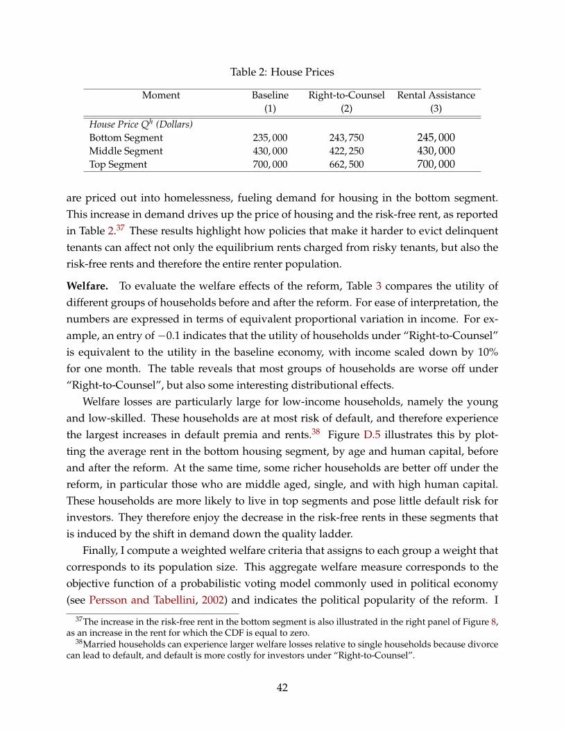
Table 2: House Prices

Moment Baseline(1)

Right-to-Counsel(2)

Rental Assistance(3)

House Price Qh (Dollars)Bottom Segment 235, 000 243, 750 245, 000Middle Segment 430, 000 422, 250 430, 000Top Segment 700, 000 662, 500 700, 000

are priced out into homelessness, fueling demand for housing in the bottom segment.This increase in demand drives up the price of housing and the risk-free rent, as reportedin Table 2.37 These results highlight how policies that make it harder to evict delinquenttenants can affect not only the equilibrium rents charged from risky tenants, but also therisk-free rents and therefore the entire renter population.

Welfare. To evaluate the welfare effects of the reform, Table 3 compares the utility ofdifferent groups of households before and after the reform. For ease of interpretation, thenumbers are expressed in terms of equivalent proportional variation in income. For ex-ample, an entry of −0.1 indicates that the utility of households under “Right-to-Counsel”is equivalent to the utility in the baseline economy, with income scaled down by 10%for one month. The table reveals that most groups of households are worse off under“Right-to-Counsel”, but also some interesting distributional effects.

Welfare losses are particularly large for low-income households, namely the youngand low-skilled. These households are at most risk of default, and therefore experiencethe largest increases in default premia and rents.38 Figure D.5 illustrates this by plot-ting the average rent in the bottom housing segment, by age and human capital, beforeand after the reform. At the same time, some richer households are better off under thereform, in particular those who are middle aged, single, and with high human capital.These households are more likely to live in top segments and pose little default risk forinvestors. They therefore enjoy the decrease in the risk-free rents in these segments thatis induced by the shift in demand down the quality ladder.

Finally, I compute a weighted welfare criteria that assigns to each group a weight thatcorresponds to its population size. This aggregate welfare measure corresponds to theobjective function of a probabilistic voting model commonly used in political economy(see Persson and Tabellini, 2002) and indicates the political popularity of the reform. I

37The increase in the risk-free rent in the bottom segment is also illustrated in the right panel of Figure 8,as an increase in the rent for which the CDF is equal to zero.

38Married households can experience larger welfare losses relative to single households because divorcecan lead to default, and default is more costly for investors under “Right-to-Counsel”.

42

find that aggregate welfare is lower under “Right-to-Counsel”.

Table 3: Equivalent Variation - “Right-to-Counsel”

Human Capital andMarital Status

Age20-35 35-50 50-65 65-80

No High-SchoolSingle −0.29 −0.07 −0.06 −0.03Married −0.14 −0.2 −0.05 −0.08

At Least High-SchoolSingle −0.06 −0.02 0.02 −0.05Married −0.17 −0.16 −0.15 0.04

Total −0.079

Notes: The table reports the one-time lump-sum transfer, as a share of monthly income, that is required to equate average household

welfare in the baseline economy to that under “Right-to-Counsel”. A negative (positive) sign means that households are better off

(worse off) in the baseline economy.

Monetary Cost. There are two monetary costs associated with “Right-to-Counsel”. Thefirst is the cost of the higher homelessness rate induced by the policy. In particular, the15 percent increase in the homelessness rate associated with “Right-to-Counsel” mapsto an additional 5, 310 homeless households. Given the monthly per-household cost ofhomelessness θ (Section 5.3), this translates to an additional 30 million dollars imposedon the city’s government every year.

The second cost is the financing costs of providing legal counsel (which is denoted byΛ in Equation 3). To estimate this cost, I first count the number of eviction cases processedannually in San Diego under “Right-to-Counsel”, which I find it to be 1, 674. I then useexternal estimates from the San Francisco Mayor’s Office of Housing and Community De-velopment (SFMOHCD) on the cost-per-case of legal counsel.39 Since San Francisco andSan Diego share similar costs of living, these estimates provide a reasonable benchmark.SFMOHCD reports the cost per 50 cases to be $222, 000. I therefore estimate the annualfinancing cost of the program to be approximately 7.4 million dollars. Taking stock, notonly does “Right-to-Counsel” dampen aggregate welfare, it is also associated with anannual monetary cost of 37.4 million dollars.

Transition dynamics. I have thus far compared the new steady state that the economyconverges to under “Right-to-Counsel” to the original steady state. Here I consider the

39The SFMOHCD is responsible for the implementation of Proposition F, the “Right-to-Counsel” legis-lation that guarantees free legal counsel to tenants facing eviction cases in San Francisco. The legislationpassed in June 2018, but has yet to be implemented.

43

transition dynamics following an unexpected passage of the reform. Rental rates on leasesthat are ongoing at the period of impact cannot be modified by investors. This meansthat households that are renting when the reform is unexpectedly announced enjoy thestronger protections against evictions, while continuing paying pre-reform rents. Alongthe transition, the homelessness rate might therefore first drop before it converges to thenew (and higher) steady state rate, in which default premia adjust to the new regime.

Figure D.6 shows that while theoretically possible, quantitatively this is not the case.The homelessness rate along the transition increases on impact and steadily increasestowards the new steady state. This is due to the high frequency at which households arehit by a moving shock. Since households move fast, they face higher rents early on alongthe transition.40

6.2 Rental Assistance

Means-tested rental assistance programs are frequently proposed as a tool for reducinghomelessness and evictions. An important conceptual difference relative to “Right-to-Counsel” is that instead of making it harder to evict tenants who have already defaulted,rental assistance lowers the likelihood that tenants default in the first place. In equilib-rium, rental assistance programs therefore lower the default premia charged by investors.In this section, I evaluate the effects of a rental assistance program that resembles theHousing Choice Voucher Program in the US.

In particular, I consider a monthly rent subsidy of $400 to households who have to-tal wealth below a threshold of $1, 000, and who rent in the bottom housing segment. Iset eligibility based on total wealth rather than only income, in resemblance with vari-ous government benefit programs that define eligibility based not only on income, butalso assets (including the Housing Choice Voucher Program and the Supplemental Secu-rity Income Benefits Program). This criteria is also more efficient in targeting householdsin need. Restricting the subsidy to the bottom segment captures the fact that rental as-sistance programs typically set an upper bound on the rent that tenants can be assistedwith. I have considered alternative specifications of the monthly subsidy and of the eli-gibility threshold, but have found this particular specification to maximize net monetarygains to the government (originating from lower homelessness costs, see below), while

40This result depends on the fact that moving rates in the model are exogenous and are unaffected by thepolicy change. One might think that when these protections are instated tenants are more likely to remainin their house to avoid paying a higher price somewhere else. While this is a concern, there is also evidenceshowing that people move for many reasons that are related to family events and job opportunities, whilemoving in order to pay a lower rent accounts for only a low share of moves (see Ihrke, 2014 for a review).

44

maintaining an aggregate welfare gain.

Rents, homelessness, and evictions. The main result is that rental assistance signifi-cantly lowers homelessness, eviction filing, and eviction rates. As illustrated in the leftpanel of Figure 10, the homelessness rate drops from 3.29 percent of the population to1.83 percent, a 45 percent decrease. Low-income households are more likely to afford tomove into a house both because the government subsidizes their rent, and because theinsurance provided by the subsidy lowers default premia in equilibrium.

Figure 10: The Effects of Rental Assistance

Notes: The CDF of rents is computed based on the observed rents in the bottom housing segment. The eviction filing rate (eviction

rate) is the share of renter households that defaulted on rent (were evicted) at least once during the past 12 months. The homelessness

rate is the share of homeless households.

To illustrate the effect on default premia, the right panel of Figure 10 plots the CDFof rents in the bottom housing segment, before (in green) and after the reform (in blue).Under rental assistance, there is a smaller mass of renters who pay high rents, reflect-ing the fact that the program essentially eliminates default risk. The eviction filing rate(top bars) and the eviction rate (middle bars) drop by approximately 75 percent under

45

rental assistance. In contrast to the case of “Right-to-Counsel”, this drop not because low-income households are priced out of the market, but rather because the subsidy lowerstheir likelihood of default.

Housing supply, house prices, and risk-free rents. Rental assistance fuels demand forhousing in the bottom housing segment, as a larger mass of low-income households canafford to rent a house. As a result, in equilibrium, housing supply and the house priceincrease in the bottom segment (see third column of Table 2). This translates to a risein the risk-free rent in the bottom segment, as investors incur higher costs when buyinghouses (the increase in the risk-free rent is illustrated in the right panel of Figure 10 byan increase in the rent for which the CDF is equal to zero). In particular, householdswho continue to rent in the bottom segment following the reform, and who were not atrisk of default in the baseline economy, pay higher risk-free rents under the reform. Thisreflects the common argument that rental assistance can raise rents by fueling demandfor housing.

Welfare. Table 4 compares the utility of different groups of households before and afterthe reform, in terms of equivalent proportional variation in income. The table reveals in-teresting heterogeneity. Poor households, namely the young and less educated, are eligi-ble for the provision and are therefore better off.41 At the same time, households who arepoor enough to rent in the bottom housing segment, but are not poor enough to qualifyfor the provision, in particular the older and less educated, are worse off. The increase inthe risk-free rent in the bottom segment induced by the policy implies that these relativelypoor (but low-risk) households pay higher rents. Figure D.7 illustrates this by plotting theaverage rent in the bottom housing segment, by age and human capital, before and afterthe reform. Finally, using the weighted welfare measure described in Section 6.1, I findthat rental assistance improves aggregate welfare.Monetary Cost. Providing rental assistance imposes costs on the local government. Us-ing the counterfactual steady state, I estimate the financing cost (Λ) of the subsidy to be81.7 million dollars every year. However, it turns out that these costs are lower than thesavings in terms of reduced homelessness. The 45 percent decrease in the homelessnessrate translates to 16, 429 fewer homeless households, implying annual savings on home-lessness expenses of 90 million dollars for the city’s government. Taking stock, the rentalassistance program results in a net gain of approximately 8 million dollars annually, ontop of it being welfare improving.

41Among the young and less educated, married households experience larger welfare gains (in terms ofequivalent proportional variation in income) relative to single households. This is because the later are sopoor that even under rental assistance some of these households remain homeless.

46

Table 4: Equivalent Variation - Rental Assistance

Human Capital andMarital Status

Age20-35 35-50 50-65 65-80

No High-SchoolSingle 0.17 0.36 −0.27 −0.04Married 0.5 0.05 −0.18 −0.03

At Least High-SchoolSingle 0.26 0 −0.09 −0.05Married 0.21 −0.02 −0.03 0

Total 0.043

Notes: The table reports the one-time lump-sum transfer, as a share of monthly income, that is required to equate median household

welfare in the baseline economy to that under the rental assistance reform. A negative (positive) sign means that households are better

off (worse off) in the baseline economy.

6.3 Eviction Moratorium

Eviction moratoria have been enacted by both the federal government and many localgovernments during the COVID-19 pandemic (see Section 2.2). While the exact details ofthese moratoria differ across time and place, they generally bar landlords from evictingdelinquent tenants. Proponents have argued that without a freeze on evictions, millionsof delinquent households would face eviction and homelessness.42 A common argumentagainst the moratorium is that it would simply delay (but not prevent) evictions, sincetenants would still be accountable for their debt once the moratorium elapses.

In this section, I evaluate the effects of a temporary eviction moratorium following anunexpected increase in the unemployment rate of the magnitude observed in the US at theonset of the COVID-19 pandemic. According to the Bureau of Labor Statistics (BLS), theunemployment rate sharply increased between February and April 2020.43 In particular,High-School dropouts experienced a 16.3 percentage point increase in unemployment,High-School graduates saw a 13.6 percentage point increase, and college graduates saw a6.4 percentage point increase.

I map these spikes in unemployment to skill-dependent job-loss probabilities, withwhich I shock employed households in the baseline steady state. I then compute thetransition dynamics following this one-time shock, for two scenarios. In the first, a 12month eviction moratorium is enacted at the time the unemployment shock hits. That is,

42According to the US Census Household Pulse Survey, which was designed to collect data on the im-pacts of COVID-19, 18.4% of renter households reported being behind on rent in December 2020. Thisnumber has slightly dropped to 15.4% in September 2021.

43https://sgp.fas.org/crs/misc/R46554.pdf.

47

the likelihood of eviction given default is set to pMRT = 0 for 12 months, before returningto its baseline value. In the second scenario, no moratorium is implemented.

Homelessness and evictions along the transition path. The main result is that themoratorium significantly reduces homelessness and evictions along the transition path.To illustrate this, Figure 11 plots the homelessness rate along the transition path follow-ing the shock, for both scenarios. Without a moratorium (in green), the homelessnessrate spikes upon impact as unemployed renters are forced to default and are evicted.It reaches approximately 3.7% of the population, before it begins to descend back to itsbaseline steady state level as households find new jobs and are able to rent again.

Figure 11: Effects of Eviction Moratorium

Notes: This figure plots the homelessness rate along the transition path, following an unexpected, one time, increase in the unemploy-

ment rate. Month 0 corresponds to the baseline steady state, and the shock hits in month 1. The blue line corresponds to an economy

in which a 12-month moratorium is enacted between months 1− 12. The green line corresponds to the no-moratorium case.

Under a moratorium (in blue), delinquent households cannot be evicted. This halt onevictions drives the downward trend in the homelessness rate for as long as the morato-

48

rium is in place. When the moratorium is lifted, the homelessness rate spikes, as delin-quent households who aren’t able to recover their debt are evicted. However, the home-lessness rate does not reach the levels of the no-moratorium case. The moratorium doesin fact prevent homelessness, not only delays it until the moratorium is lifted.

To illustrate the effects of the moratorium on evictions, Figure 12 plots the eviction-to-default rate along the transition, with and without the moratorium. Without a morato-rium (in green), nearly all default spells end with an eviction, as is the case in the baselinesteady state. Under a moratorium (in blue) a large number of delinquent households areable to avoid eviction by repaying their debt. The eviction-to-default rate is substantiallylower than one, especially during the first part of the moratorium. By providing delin-quent tenants more time to find new jobs, the moratorium is able to prevent evictions, notonly delay them until the moratorium is lifted.

Figure 12: Eviction-to-Default Rates with and without a Moratorium

Notes: This figure plots the eviction-to-default rate along the transition path, following an unexpected, one time, increase in the

unemployment rate. The blue line corresponds to an economy in which a 12-month moratorium is enacted between months 1− 12.

The green line corresponds to the no-moratorium case.

49

The temporary nature of the moratorium. It is informative to compare the effects of themoratorium to the effects of “Right-to-Counsel”, both of which make it harder to evictdelinquent tenants. While “Right-to-Counsel” is unable to prevent evictions of delin-quent households, and leads to an increase in the homelessness rate, an eviction mora-torium successfully lowers both. The first important distinction is that the moratoriumis used as a temporary measure, while “Right-to-Counsel” is a permanent change in theeviction regime. The temporary nature of the moratorium implies that it leads to onlymild increases in default premia and rents, since default costs for investors are higher foronly a limited amount of time. When setting the rent on new leases, investors are lessworried about future defaults if they anticipate that the moratorium will soon be lifted.

The composition of households who default as a result of the aggregate unemploy-ment shock is also different relative to normal times. As documented in the BLS data,households across the human capital distribution, some of which are highly unlikelyto lose their job and default under normal circumstances, lost their job at the onset ofCOVID-19. However, the new jobs that High-School and College graduates find involvehigher pay relative to the jobs landed by High-School dropouts, who are those typicallyunemployed in normal times. In this sense, the default risk along the recovery path is onaverage less persistent and easier to smooth with more time. Making it harder to evictdelinquent tenants is more effective when default risk is more temporary in nature.

7 Conclusion

Despite the wide policy interest, little is known on the equilibrium effects of eviction andhomelessness policies, when rents and housing supply can adjust. This paper quantita-tively evaluates these policies in a dynamic equilibrium model of the rental markets in acity, in which households can default on rent and face the risk of eviction and homeless-ness. The model is quantified to San Diego County and is estimated to match micro dataon evictions, and homelessness, as well as the risk dynamics that drive defaults on rent. Ithen use the quantified model for counterfactual analysis.

I find that “Right-to-Counsel” drives up default premia so much that homelessnessrises by 15 percent in equilibrium. While lawyers make it harder to evict delinquent ten-ants, they are unable to prevent their eviction. The shocks that drive defaults, namelyjob-losses and divorces, are associated with persistent income consequences and there-fore cannot easily be smoothed across time. Low-income households suffer the largestwelfare losses, since they experience the largest increases in rent and are priced out ofthe market. At the same time, some richer households are better-off, as the risk-free rent

50

they pay is lower due to the fall in housing supply and house price induced by the policy.Overall, “Right-to-Counsel” dampens aggregate welfare and is associated with an annualmonetary cost of 37.4 million dollars to the County of San Diego.

Means-tested rental assistance is a more promising solution. It reduces homelessnessby 45 percent and the eviction filing rate by approximately 75 percent. The insuranceprovided by the subsidy lowers the likelihood of default rather than making it harder toevict tenants who have already defaulted. Low-income households, who are eligible forthe assistance, are the main beneficiaries. Some richer households are worse-off , sincethe risk-free rent that they pay is higher, reflecting the increase in housing supply andhouse price induced by the policy. Rental assistance improves aggregate welfare and isassociated with net monetary gains: the cost of subsidizing rent is lower than the savingsin terms of lower expenditure on homelessness.

Finally, I evaluate the effects of enacting a temporary moratorium on evictions in re-sponse to an unemployment shock of the magnitude observed in the US at the onset ofthe COVID-19 pandemic. I find that the moratorium prevents homelessness and evictionsalong the transition path. The temporary nature of the moratorium is key, as it impliesthat the moratorium leads to only mild increases in rents.

51

ReferencesAbowd, John M, and David Card. 1989. “On the covariance structure of earnings and hours changes.”

Econometrica: Journal of the Econometric Society, 411–445.

Aguiar, Mark, and Gita Gopinath. 2006. “Defaultable debt, interest rates and the current account.” Journalof international Economics, 69(1): 64–83.

An, Xudong, Stuart A Gabriel, and Nitzan Tzur-Ilan. 2021. “COVID-19 Rental Eviction Moratoria andHousehold Well-Being.” Available at SSRN 3801217.

Arellano, Cristina. 2008. “Default risk and income fluctuations in emerging economies.” American EconomicReview, 98(3): 690–712.

Baum-Snow, Nathaniel, and Justin Marion. 2009. “The effects of low income housing tax credit develop-ments on neighborhoods.” Journal of Public Economics, 93(5-6): 654–666.

Benfer, Emily A, David Vlahov, Marissa Y Long, Evan Walker-Wells, JL Pottenger, Gregg Gonsalves,and Danya E Keene. 2021. “Eviction, health inequity, and the spread of COVID-19: housing policy as aprimary pandemic mitigation strategy.” Journal of Urban Health, 98(1): 1–12.

Boyer-Vine, Ms Diane F, Mr Daniel Alvarez, Mr E Dotson Wilson, Dear Ms Boyer-Vine, Mr Alvarez, andMr Wilson. 2017. “JUDICIAL COUNCIL OF CALIFORNIA.”

Burgard, Sarah A, Kristin S Seefeldt, and Sarah Zelner. 2012. “Housing instability and health: findingsfrom the Michigan Recession and Recovery Study.” Social science & medicine, 75(12): 2215–2224.

Chatterjee, Satyajit, Dean Corbae, Makoto Nakajima, and José-Víctor Ríos-Rull. 2007. “A quantitativetheory of unsecured consumer credit with risk of default.” Econometrica, 75(6): 1525–1589.

Corbae, Dean, and Erwan Quintin. 2015. “Leverage and the foreclosure crisis.” Journal of Political Economy,123(1): 1–65.

Davis, Morris A, and François Ortalo-Magné. 2011. “Household expenditures, wages, rents.” Review ofEconomic Dynamics, 14(2): 248–261.

Deaton, Angus, and Christina Paxson. 1994. “Intertemporal choice and inequality.” Journal of political econ-omy, 102(3): 437–467.

De Nardi, Mariacristina. 2004. “Wealth inequality and intergenerational links.” The Review of EconomicStudies, 71(3): 743–768.

Desmond, M, A Gromis, L Edmonds, J Hendrickson, K Krywokulski, L Leung, and A Porton. 2018.“Eviction lab national database: Version 1.0.”

Desmond, Matthew, and Rachel Tolbert Kimbro. 2015. “Eviction’s fallout: housing, hardship, and health.”Social forces, 94(1): 295–324.

52

Desmond, Matthew, Weihua An, Richelle Winkler, and Thomas Ferriss. 2013. “Evicting children.” SocialForces, 92(1): 303–327.

Diamond, Rebecca, Tim McQuade, and Franklin Qian. 2019. “The effects of rent control expansion on ten-ants, landlords, and inequality: Evidence from San Francisco.” American Economic Review, 109(9): 3365–94.

Eaton, Jonathan, and Mark Gersovitz. 1981. “Debt with potential repudiation: Theoretical and empiricalanalysis.” The Review of Economic Studies, 48(2): 289–309.

Ellen, Ingrid Gould, Katherine O’Regan, Sophia House, and Ryan Brenner. 2020. “Do Lawyers Matter?Early Evidence on Eviction Patterns After the Rollout of Universal Access to Counsel in New York City.”Housing Policy Debate, 1–22.

Glaeser, Edward L, and Erzo FP Luttmer. 2003. “The misallocation of housing under rent control.” AmericanEconomic Review, 93(4): 1027–1046.

Gourinchas, Pierre-Olivier, and Jonathan A Parker. 2002. “Consumption over the life cycle.” Econometrica,70(1): 47–89.

Greiner, D James, Cassandra Wolos Pattanayak, and Jonathan Hennessy. 2013. “The limits of unbundledlegal assistance: a randomized study in a Massachusetts district court and prospects for the future.”Harv. L. rev., 126: 901.

Greiner, D James, Cassandra Wolos Pattanayak, and Jonathan Philip Hennessy. 2012. “How effectiveare limited legal assistance programs? A randomized experiment in a Massachusetts housing court.” ARandomized Experiment in a Massachusetts Housing Court (September 1, 2012).

Guren, Adam M, Arvind Krishnamurthy, and Timothy J McQuade. 2021. “Mortgage design in an equi-librium model of the housing market.” The Journal of Finance, 76(1): 113–168.

Guvenen, Fatih. 2007. “Learning your earning: Are labor income shocks really very persistent?” AmericanEconomic Review, 97(3): 687–712.

Guvenen, Fatih, Fatih Karahan, Serdar Ozkan, and Jae Song. 2015. “What do data on millions of USworkers reveal about life-cycle earnings risk?” National Bureau of Economic Research.

Heathcote, Jonathan, Fabrizio Perri, and Giovanni L Violante. 2010. “Unequal we stand: An empiricalanalysis of economic inequality in the United States, 1967–2006.” Review of Economic dynamics, 13(1): 15–51.

Humphries, John Eric, Nicholas S Mader, Daniel I Tannenbaum, and Winnie L van Dijk. 2019. “Doeseviction cause poverty? Quasi-experimental evidence from Cook County, IL.” National Bureau of Eco-nomic Research.

Ihrke, David. 2014. Reason for Moving: 2012 to 2013. US Department of Commerce, Economics and StatisticsAdministration, US Census Bureau.

53

Jeske, Karsten, Dirk Krueger, and Kurt Mitman. 2013. “Housing, mortgage bailout guarantees and themacro economy.” Journal of Monetary Economics, 60(8): 917–935.

Jowers, Kay, Christopher Timmins, Nrupen Bhavsar, Qihui Hu, and Julia Marshall. 2021. “Housing pre-carity & the covid-19 pandemic: Impacts of utility disconnection and eviction moratoria on infectionsand deaths across us counties.” National Bureau of Economic Research.

Klein, Paul, and Irina A Telyukova. 2013. “Measuring high-frequency income risk from low-frequencydata.” Journal of Economic Dynamics and Control, 37(3): 535–542.

Landvoigt, Tim, Monika Piazzesi, and Martin Schneider. 2015. “The housing market (s) of San Diego.”American Economic Review, 105(4): 1371–1407.

Livshits, Igor, James MacGee, and Michele Tertilt. 2007. “Consumer bankruptcy: A fresh start.” AmericanEconomic Review, 97(1): 402–418.

Mast, Evan. 2019. “The Effect of New Market-Rate Housing Construction on the Low-Income HousingMarket.” Upjohn Institute WP, 19–307.

Mateyka, Peter, and Matthew Marlay. 2011. “Residential Duration by Tenure, Race and Ethnicity: 2009.”

Meghir, Costas, and Luigi Pistaferri. 2004. “Income variance dynamics and heterogeneity.” Econometrica,72(1): 1–32.

Meyer, Bruce D, Angela Wyse, Alexa Grunwaldt, Carla Medalia, and Derek Wu. 2021. “Learning aboutHomelessness Using Linked Survey and Administrative Data.” National Bureau of Economic Research.

Persson, Torsten, and Guido Tabellini. 2002. Political economics: explaining economic policy. MIT press.

Phinney, Robin, Sheldon Danziger, Harold A Pollack, and Kristin Seefeldt. 2007. “Housing instabilityamong current and former welfare recipients.” American Journal of Public Health, 97(5): 832–837.

Pruitt, Seth, and Nicholas Turner. 2020. “Earnings Risk in the Household: Evidence from Millions of USTax Returns.” American Economic Review: Insights, 2(2): 237–54.

Saiz, Albert. 2010. “The geographic determinants of housing supply.” The Quarterly Journal of Economics,125(3): 1253–1296.

Seron, Carroll, Gregg Van Ryzin, Martin Frankel, and Jean Kovath. 2014. “17. The Impact of Legal Coun-sel on Outcomes for Poor Tenants in New York City’s Housing Court: Results of a Randomized Experi-ment.” In The Law and Society Reader II. 159–165. New York University Press.

Sullivan, Teresa A, Elizabeth Warren, and Jay Lawrence Westbrook. 1999. As we forgive our debtors:Bankruptcy and consumer credit in America. Beard Books.

54

Appendix

Contents

A “Right-to-Counsel” in New York City 56

B Bellman Equations 60B.1 Household Problem . . . . . . . . . . . . . . . . . . . . . . . . . . . . . . . . . 60B.2 Investor Zero Profit Condition . . . . . . . . . . . . . . . . . . . . . . . . . . . 63B.3 Risk-free Rent and Default Premia - an Example . . . . . . . . . . . . . . . . 64

C Income: Facts and Estimation 66C.1 Data and Facts . . . . . . . . . . . . . . . . . . . . . . . . . . . . . . . . . . . . 66

C.1.1 Average Life-Cycle Profile . . . . . . . . . . . . . . . . . . . . . . . . . 67C.1.2 Standard Deviation of Earnings Growth . . . . . . . . . . . . . . . . . 68C.1.3 Unemployment risk . . . . . . . . . . . . . . . . . . . . . . . . . . . . 69

C.2 Income Process Estimation . . . . . . . . . . . . . . . . . . . . . . . . . . . . . 70

D Additional Figures and Tables 74

55

A “Right-to-Counsel” in New York City

New York was the first jurisdiction to enact a city-wide “Right-to-Counsel” legislation.The program began with the Expanded Legal Services (ELS) pilot program in ten ZIPcodes in early 2016 (which I refer to as T1 Zip codes). Through ELS, legal representationin eviction cases was provided for individuals living in those ZIP Codes with householdincomes of up to 200 percent of the federal poverty line (NYC Office of Civil Justice,2016). Zip codes were selected partly based on rates of shelter entry. In August 2017, thecity council approved a “Universal Access to Counsel” (UAC) legislation, providing freelegal representation to all income-qualified tenants facing evictions. UAC was rolled outin phases. In October 2017, five additional Zip codes (T2) were added to the ten ELS Zipcodes, based on several characteristics such as shelter entries and eviction case volumes.Five additional Zip codes (T3) were added in November 2018 and five additional Zipcodes (T4) were added in December 2019. Remaining ZIP codes (referred to as C Zipcodes) are scheduled to be added by 2022.

Ellen et al. (2020) exploit the gradual rollout of UAC and compare eviction patternsacross the five cohorts of ZIP codes. They find that UAC had indeed increased the shareof eviction cases in which tenants are represented by lawyers. In terms of case outcomes,legal counsel is found to slightly decrease the share of cases that end with an evictionwarrant being executed. It is important to note that evictions can happen through settle-ments between the landlord and tenant, and even when an eviction judgement is made,most tenants leave the dwelling before an actual warrant is executed. The length of theeviction proceeding is found to have increased in treated Zip codes. Ellen et al. (2020)highlight that since the program is in its early rollout stages, results should be regardedas preliminary.

Nevertheless, the sequential rollout of the program provides an opportunity to exam-ine whether the legislation had effects on rents. To do so, I use the Zillow Observed RentIndex (ZORI) which is reported at the ZIP code level and at a monthly frequency.44 FigureA.1 plots the log-difference in average rent between each of the four treated ZIP code co-horts and the non-treated cohort. The patterns reveal little indication for shifts in trendsassociated with the rollout of UAC.

However, as reported by Ellen et al. (2020), while there seem to be little systematic dif-ferences across ZIP Codes based on timing of implementation, they are different relativeto the non-treated cohort in terms of observed characteristics. To account for these differ-ences, I compare the average rent in the ZIP codes that began receiving treatment at the

44For more details see https://www.zillow.com/research/methodology-zori-repeat-rent-27092/

56

start of 2016 to a synthetic control group of non-treated ZIP codes, constructed based on2014 Census data on median household income, median rent, demographic composition(percentage of black households and of hispanic households), share of renter households,and share of households with a High-School degree. Figure A.2 suggests no meaningfuldifferences following the implementation.

When interpreting these results, it is important to note that the UAC program is stillin its early rollout stages, and any analysis of its effects on prices should be consideredpreliminary. Furthermore, New York City’s unique legal environment limits the gener-alizability of the findings to other jurisdictions. In particular, nearly half of rental unitsin New York are under rent control regulations, which provide landlords with strong in-centives to evict tenants based on false allegations in order to raise future rents. Ownersof rent-controlled dwellings are not allowed to raise rents by more than a certain incre-ment when the tenant occupying the unit wishes to extend the lease. However, when anew tenant enters, rents can be raised more flexibly. Furthermore, once rent exceeds acertain threshold, the dwelling is no longer considered rent-controlled. In this environ-ment, lawyers can protect tenants from unlawful evictions and therefore prevent futurerent increases. The fact that we observe no effect of rent suggests there may be anotherforce that acts to increase rents, namely that landlords charge higher rents in response tothe higher costs from longer eviction proceedings.

57

Figure A.1: Log-Difference in Rents Relative to Non-UAC ZIP Codes

Notes: Each line corresponds to the difference in the (log) average ZORI across ZIP codes in a particular treatment cohort, relative to

the (log) average rent in non-treated ZIP codes (C). The vertical lines correspond to the timing in which different cohorts were added

to the UAC program.

58

Figure A.2: Difference in Rents Relative to Synthetic Control Group of Non-UAC ZIP Codes

Notes: The blue solid line corresponds to the average ZORI across ZIP codes in the T1 cohort. The dashed green line corresponds to the

ZORI of a synthetic control group of non-treated ZIP codes (cohort C). The synthetic group is constructed by searching for a weighted

combination of non-treated ZIP codes chosen to approximate the T1 group of ZIP codes in terms of median household income, median

rent, demographic composition (percentage of black households and of hispanic households), share of renter households, and share

of households with a High-School degree in 2014.

59

B Bellman Equations

In this section, I specify the Bellman equations that correspond to the household’s prob-lem in Section 4.3 and the investor zero profit condition in Section 4.4. To do so, it isuseful to denote by α = (1− σ)(1− δ) the probability that neither a moving shock nor adepreciation shock are realized between time t and time t + 1.

B.1 Household Problem

For clarity, throughout this section I distinguish the problem of a household of age a < Afrom the problem of a household of age a = A.

Non-occupiers

The lifetime utility of a household that begins period t without a house (Ot = out) and isof age at < A is given by

Voutt (at, yt, zt, wt, mt, e) =

maxst,ct,bt

U(ct, st) + βαEΓt+1

[Vocc

t+1 (at + 1, zt+1, wt+1, mt+1, e, h, q, 0)]+ st = h ∈ H

+β (1− α)EΓt+1

[Vout

t+1

(at + 1, yt+1, zt+1, wt+1, mt+1, e

)]U(ct, st) + βEΓt+1

[Vout

t+1 (at + 1, yt+1, zt+1wt+1, mt+1, e)]

st = u

s.t. ct + bt =

wt − q st = h ∈ H

wt st = u,

q = qstt (at, yt, wt),

wt+1 = (1 + r)bt + yt+1,

ct ≥ 0, bt ≥ 0, (5)

where ct is numeraire consumption, bt are savings, Γt+1 = mt+1, zt+1, ut+1 are the riskfactors that determine the wealth at the next period, and Vocc

t+1 is the lifetime utility of ahousehold that begins the next period occupying a house (see below). The lifetime utilityof a household that begins period t without a house and is of age at = A is given by

60

Voutt (A, yt, zt, wt, mt, e) =

maxst,ct,bt

U(ct, st) + EΓt+1

[νbeq(wt+1)

]s.t. ct + bt =

wt − q st = h ∈ H

wt st = u,

q = qstt (A, yt, wt),

wt+1 = (1 + r)bt + yt+1,

ct ≥ 0, bt ≥ 0. (6)

Occupiers

The lifetime utility of a household that begins period t under an ongoing lease (Ot = occ)and is of age at < A is given by

Vocct (at, zt, wt, mt, e, h, q, kt) =

maxdt,ct,bt

U(ct, h) + βαEΓt+1

[Vocc

t+1 (at + 1, zt+1, wt+1, mt+1, e, h, q, 0)]+ dt = 0

β(1− α)EΓt+1

[Vout

t+1 (at + 1, yt+1, zt+1, wt+1, mt+1, e)]

(1− p)

U(ct, h) + βαEΓt+1

[Vocc

t+1 (at + 1, zt+1, wt+1, mt+1, e, h, q, kt+1)]+ dt = 1

β(1− α)EΓt+1

[Vout

t+1 (at + 1, yt+1, zt+1, wt+1 −minφkt+1, wt+1, mt+1, e)]

+

pVevictedt (at, zt,wt, mt,e, kt)

s.t. ct + bt =

wt − q− kt dt = 0

wt dt = 1,

wt+1 = (1 + r)bt + yt+1,

ct ≥ 0, bt ≥ 0,

kt+1 = (1 + r)(kt + q), (7)

where Vevictt is the lifetime utility of an evicted household (and is described below). A

household that does not default pays the per-period rent as well as any outstanding debtit might have accrued from previous periods. It begins the next period occupying the

61

house with no outstanding debt, unless a moving or depreciation shock hit, in which itbegins the next period as a non-occupier. A household that defaults and is not evictedbegins the next period occupying the house with accrued debt, unless a moving or depre-ciation shock hit, in which it begins the next period as a non-occupier and pays a share φ

of its rental debt (or its entire wealth, if wealth is insufficient).I assume that households that default in the last period of life and are not evicted pay afraction φ of their debt in the period of death (or their entire wealth, if wealth is insuffi-cient). The lifetime utility of a household that begins the period occupying a house and isof age at = A therefore reads as

Vocct (A, zt, wt, mt, e, h, q, kt) =

maxdt,ct,bt

U(ct, h) + βEΓt+1

[νbeq(wt+1)

]dt = 0

(1− p)(U(ct, h) + βEΓt+1

[νbeq(wt+1 −minφkt+1, wt+1)

])dt = 1

pVevictedt (A, zt,wt, mt,e, kt)

s.t. ct + bt =

wt − q− kt dt = 0

wt dt = 1,

wt+1 = (1 + r)bt + yt+1,

ct ≥ 0, bt ≥ 0,

kt+1 = (1 + r)(kt + q). (8)

Evicted

The lifetime utility of a household that is evicted at time t and is of age at < A is given by

Vevictt (at, zt,wt, mt,e, kt) =

maxct,bt

U(ct, u) + βEΓt+1

[Vout

t+1 (at + 1, yt+1, zt+1wt+1, mt+1, e)]

s.t. ct + bt ≤ (1− λ)(wt −minφkt, wt),wt+1 = (1 + r)bt + yt+1,

ct ≥ 0, bt ≥ 0. (9)

The lifetime utility of a household that is evicted at time t and is of age at = A is given by

62

Vevictt (A, zt,wt, mt,e, kt) =

maxct,bt

U(ct, u) + βEΓt+1

[νbeq(wt+1)

]s.t. ct + bt ≤ (1− λ)(wt −minφkt, wt),

wt+1 = (1 + r)bt + yt+1,

ct ≥ 0, bt ≥ 0. (10)

B.2 Investor Zero Profit Condition

The zero profit condition on a lease that starts in period t on a house of quality h that isrented to a household with observables (at, yt, wt), for at < A, reads as

0 = −Qht + qh

t (at, yt, wt)− τh +(1− δ)σ

1 + rQh

t+1+

α

1 + r×E

[Πocc

t+1

(at + 1, zt+1, wt+1, mt+1, e, h, qh

t (at, yt, wt), 0)]

, (11)

where the first line corresponds to the net revenue at period t and the discounted valueof selling the house if the lease terminates between period t and period t + 1. The secondline corresponds to the value of an ongoing lease in period t + 1.

For a household of age at = A the condition is simply

0 = −Qht + qh

t (A, yt, wt)− τh +(1− δ)

1 + rQh

t+1.

The Value of an Ongoing Lease

The value from a lease that is ongoing at the beginning of period t, on a house of qualityh, with an occupier household who has accumulated previous debt of kt, and who has

63

contemporary characteristics (at, zt, wt, mt, e), where at < A is given by45

Πocct (at, zt, wt, mt, e, h, q, kt) =

q + kt − τh+ docct = 0

α1+r E

[Πocc

t+1 (at + 1, zt+1, wt+1, mt+1, e, h, q, 0)]+ (1−δ)σ

1+r Qht+1

(1− p)×−τh + α

1+r E

[Πocc

t+1 (at + 1, zt+1, wt+1, mt+1, e, h, q, kt+1)

]+ docc

t = 1

(1−δ)σ1+r

(E [min φkt+1, wt+1] + Qh

t+1)+ δ

1+r E [min φkt+1, wt+1]+

p×(

minφkt, wt+ (1−δ)σ1+r Qh

t+1

)(12)

s.t. kt+1 = (1 + r)(kt + q),

where docct is the default decision of an occupier household with state at, zt, wt, mt, e, h, q, kt.46

The continuation value from an ongoing lease with a household of age at = A reads as

Πocct (A, zt, wt, mt, e, h, q, kt) =

q + kt − τh + 1−δ1+r Qh

t+1 docct = 0

(1− p)×(−τh + 1

1+r EΓt+1 [min φkt+1, wt+1])+ docc

t = 1

p×minφkt, wt+ 1−δ1+r Qh

t+1

s.t. kt+1 = (1 + r)(kt + q).

B.3 Risk-free Rent and Default Premia - an Example

In this section, I provide an example for how rent can be decomposed into a risk-freerent component and a default premium component. For clarity, I consider the stationaryequilibrium case, where prices and policy functions are time-independent, and I focus

45 Because investors observe the household’s age, income and wealth at time t, but behavior at time t + 1depends on future state variables, expectations on future states are formed conditional on the age, incomeand wealth at time t and the time t distribution of households over the state space.

46I assume that when the lease terminates due to eviction, the investor can sell the house only in thefollowing period, and collects only a fraction σ of the resale price. This technical assumption is made inorder to ensure that the investor does not benefit from default through a potential earlier resale of the houseand lower depreciation costs.

64

on a lease that starts when a household is of age A− 1. Furthermore, I assume that thehousehold’s wealth at the period of death is larger than the per-period rent, which impliesthat the investor collects a fraction φ of the accrued debt in case the household defaultsin the last period of life. Given that the household has income y and wealth w, the zeroprofit condition reads as

0 = −Qh + qh(A− 1, y, w)− τh +(1− δ)σ

1 + rQh+

α

1 + rE

[(1− docc)

(qh(A− 1, yt, wt)− τh +

(1− δ)

1 + rQh)+

docc(1− p)(−τh +

(1− δ)

1 + rQh + φqh(A− 1, y, w)

)+

docc p(1− δ)

1 + rQh

],

where docc is the default decision of the occupier household at age A. Rearranging, wecan solve for the per-period rent specified by the lease:

qh(A− 1, y, w) =(1 +

α

1 + r[1−E(docc)× (1− φ(1− p))]

)−1

×[Qh(

1− (1− δ)σ

1 + r− α

1 + r(1− δ)

1 + r

)+

τh(

1 +α

1 + r(1−E(docc)p)

)].

The risk-free rent is defined as the rent that is charged from a household for which defaultrisk is zero. In this case, it is given by

qhRF = τh +

(1 +

α

1 + r

)−1(1− (1− δ)σ

1 + r− α

1 + r(1− δ)

1 + r

)×Qh.

It is an increasing function of the house price Qh and the per-period cost τh.The default premium is defined as qh(A− 1, y, w)− qh

RF. It is straightforward to verifythat it is increasing with p and φ, i.e. when it is harder and more expensive to evict adelinquent tenant, and when the household’s default risk is higher.47

47Since φ ≤ 1, 1− φ(1− p) ≥ p, so that an increase in E(docc) implies the an increase in qh(A− 1, y, w).

65

C Income: Facts and Estimation

This section has two goals. First, it complements Section 3.2 by presenting additionalfacts on the income dynamics associated with defaults on rent. In Section 3.2, I showedthat (1) job-loss and divorce are the main risk factors driving defaults, (2) young and lesseducated households are more likely to lose their job and to divorce, and (3) divorce isassociated with higher job-loss risk. In this section, I show that (1) young, less educated,and single households are poorer on average, and (2) less educated, single, and especiallyindividuals who recently divorced, draw their labor earnings from a more risky distribu-tion. Second, I discuss the income process estimation, which targets and matches the factsdocumented in Section 3.2 and in this Section.

C.1 Data and Facts

The main data source I use in this section is the Panel Study of Income Dynamics (PSID).The labor earnings data are drawn from the last 38 annual and bi-annual waves of PSIDcovering the period from 1970 to 2017.48 My sample consists of head of households be-tween the ages of 20 and 60 who live in an urban area in California. I define labor in-come as total reported labor income, social security income, and transfers, for both headof household and if present his spouse.49 I include an individual into the sample if itsatisfies the following conditions for at least 10 (not necessarily consecutive) years: (1) re-ported positive income; (2) earnings were below a preset maximum (to filter out extremeobservations). These criteria are similar to the ones used in previous studies (Abowd andCard, 1989; Meghir and Pistaferri, 2004; Guvenen, 2007, among others). For each obser-vation I record the lagged earnings as the earnings of the head of household to which theindividual belonged to in previous years

Consistent with the CPS sample construction discussed in Section 3.1, I allocate in-dividuals in the PSID sample to three human capital groups using information on thehighest grade completed: High-School dropouts (denoted by e = 1), High-School gradu-ates (those with a High-School diploma, but without a college degree, denoted by e = 2),and college graduates (denoted by e = 3). I also keep track of whether the individualis single (denoted by m = 0) or married (m = 1) in each year. Consistent with the CPSsample, an individual is classified as married if she is cohabiting with a spouse, whetheror not legally married.

48The PSID was conducted annually up until 1997 and bi-annually thereafter.49Labor income defined this way was deflated using the Consumer Price Index, with 2015 as base-year.

66

C.1.1 Average Life-Cycle Profile

I first examine how the average earnings depend on age, human capital and marital sta-tus. I follow the standard procedure in the literature (e.g., Deaton and Paxson, 1994) andregress log earnings on a full set of age and cohort dummies, as well as additional con-trols including family size and gender. Estimated independently for each human capitalgroup, I allow age dummies to depend on marital status and denote them by da,m,e. Foreach human capital and marital status group, I fit a second-degree polynomial to the agedummies and denote its parameters by f0(e, m), f1(e, m), and f2(e, m). Figure C.1 plots theage dummies together with the polynomial fits and illustrates that young, High-Schooldropouts (in green), and singles (Panel (a)) are poorer on average. High-School dropoutsand single households also face lower growth rates over the life cycle.

Figure C.1: Age Profile of Log Earnings

Notes: Dots correspond to estimated age-dummies from a regression of log earnings on a full set of age and cohort dummies, as

well as family size and gender. Regressions are estimated independently for each human capital group, and I allow age-dummies

to depend on marital status. For each human capital and marital status group, I normalize the age dummies such that at age 20 the

dummy is equal to the empirical average log-earnings. “no HS” corresponds to High-School dropouts (e = 1), “HS” corresponds to

individuals who completed High-School but not college (e = 2), and “College” corresponds to college graduates (e = 3). Lines are a

second degree polynomial fit to the age dummies.

67

C.1.2 Standard Deviation of Earnings Growth

Next, I focus on the second moment of the earnings growth distribution, which is infor-mative for how income risk varies with household characteristics. Let Yi

t,a,m,e denote theannual earnings in year t of individual i who is a years old, is of marital status m andbelongs to the human capital group e. Following Guvenen et al. (2015), for computingmoments of earnings growth I work with the time difference of ui

t,a,m,e which is log earn-ings net of the age, marital status, and human capital group effects. Thus:

4kuit,a,m,e ≡

(ui

t,a,m,e − uit−k,a−k,m−k,e

)=(

log Yit,a,m,e − da,m,e

)−(

log Yit−k,a−k,m−k,e − da−k,m−k,e

).

For each lag k = 1, 2, 3, I bundle observations into nine groups, three for each level ofhuman capital. The first consists of individuals who are married (m = 1), the second ismade of single individuals (m = 0) who were also single k years ago (m−k = 0), and thethird group is of single individuals who were married k years ago (m−k = 1) and divorcedin the meantime. For each lag k, and for each of the nine groups, I compute the cross-sectional standard deviation of4kui

t,a,m,e for each year t = 1970, 1981, ..., 2017 and averagethese across all years. I denote this moment by SD

(4k(e, m, m−k)

). This approach allows

me to examine whether income risk varies with human capital and across married, single,and recently divorced individuals.50

Figure C.2 plots the one-year, two-year and three-year standard deviation of the earn-ings growth distribution. The first finding is that individuals with High-School dropoutsface more income risk.51 Second, conditional on human capital, individuals who haverecently divorced (in blue) face more income risk relative to other single households (inred) and married households (in green), and the magnitude of this pattern is especiallypronounced for the low-skilled. Divorce can be associated with high income volatility if,for example, individuals do not immediately adapt their labor supply to that expectedfrom single individuals. My third finding is that married individuals face less risk thansingle and divorced. Intuitively, spousal earnings provide a form of insurance againstshocks (Pruitt and Turner, 2020).

50I do not distinguish between married couples who were single vs. married k years ago, since marriageevents are not a driver of evictions.

51This result is similar to Meghir and Pistaferri (2004), who find that household with low educationexperience more income volatility, and also to Guvenen et al. (2015), who find that, households with higherlevels of recent earnings experience less volatility.

68

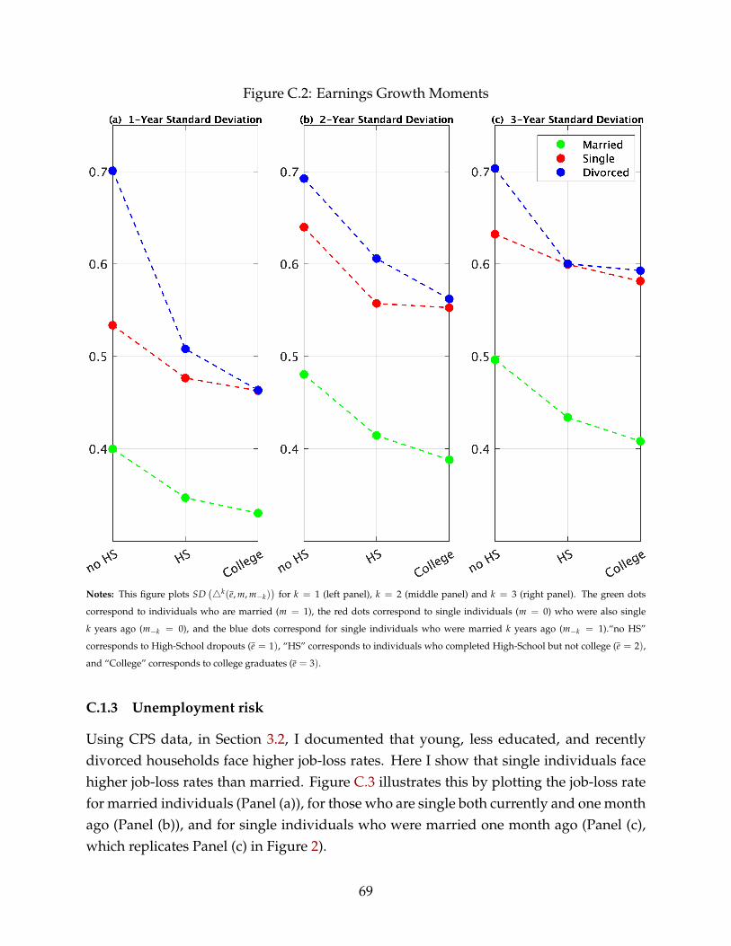
Figure C.2: Earnings Growth Moments

Notes: This figure plots SD(4k(e, m, m−k)

)for k = 1 (left panel), k = 2 (middle panel) and k = 3 (right panel). The green dots

correspond to individuals who are married (m = 1), the red dots correspond to single individuals (m = 0) who were also single

k years ago (m−k = 0), and the blue dots correspond for single individuals who were married k years ago (m−k = 1).“no HS”

corresponds to High-School dropouts (e = 1), “HS” corresponds to individuals who completed High-School but not college (e = 2),

and “College” corresponds to college graduates (e = 3).

C.1.3 Unemployment risk

Using CPS data, in Section 3.2, I documented that young, less educated, and recentlydivorced households face higher job-loss rates. Here I show that single individuals facehigher job-loss rates than married. Figure C.3 illustrates this by plotting the job-loss ratefor married individuals (Panel (a)), for those who are single both currently and one monthago (Panel (b)), and for single individuals who were married one month ago (Panel (c),which replicates Panel (c) in Figure 2).

69

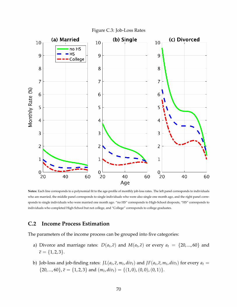
Figure C.3: Job-Loss Rates

Notes: Each line corresponds to a polynomial fit to the age-profile of monthly job-loss rates. The left panel corresponds to individuals

who are married, the middle panel corresponds to single individuals who were also single one month ago, and the right panel corre-

sponds to single individuals who were married one month ago. “no HS” corresponds to High-School dropouts, “HS” corresponds to

individuals who completed High-School but not college, and “College” corresponds to college graduates.

C.2 Income Process Estimation

The parameters of the income process can be grouped into five categories:

a) Divorce and marriage rates: D(at, e) and M(at, e) or every at = 20, ..., 60 ande = 1, 2, 3.

b) Job-loss and job-finding rates: JL(at, e, mt, divt) and JF(at, e, mt, divt) for every at =

20, ..., 60, e = 1, 2, 3 and (mt, divt) = (1, 0), (0, 0), (0, 1).

70

c) Monthly unemployment benefits yunemp(at, e, mt) for every at = 20, ..., 60, e =

1, 2, 3 and mt = 0, 1.

d) Retirement income yRet(e, mt) for every e = 1, 2, 3 and mt = 0, 1.

e) The deterministic age profile:

f (at, e, mt) = f0(e, mt) + f1(e, mt)at + f2(e, mt)a2t ,

for every e = 1, 2, 3 and mt = 0, 1.

f) The autocorrelation and variance of the persistent income component zt, and thevolatility of the transitory component ut: ρ(e, mt, divt), σ2

ε (e, mt, divt) and σ2u(e, mt, divt)

for e = 1, 2, 3 and (mt, divt) = (1, 0), (0, 0), (0, 1).

Independently Estimated Income Parameters

I calculate the monthly marriage and divorce probabilities from the Current PopulationSurvey (CPS) sample described in Section 3.1. Divorce rates discussed in Section 3.2 andare plotted in Panel (b) of Figure 2. Similarly, for each age and human capital group, Icompute the marriage rate as the share of observations where the lagged marital statusreads as single, but the current marital status is married. Job-loss and job-finding rates arecomputed from the CPS, as described in Section C.1.3. Monthly unemployment benefitsin California are roughly 60% of the monthly wage during the highest paid quarter of theyear prior to unemployment, up to a certain maximum level52. I use the PSID sampleto impute the unemployment benefits from the observed annual labor income by assum-ing it is uniformly distributed across months. I then average across age, human capitaland marital status. Retirement income is calculated as the average monthly income ofindividuals aged 60 or above, by human capital and marital status.

SMM Estimation

The remaining income parameters are jointly estimated using a Simulated Method ofMoments approach. Since the income process is monthly but the PSID income data isannual, the usual GMM estimation methods, that require exact analytical formulas for theannual covariance moments, cannot be applied (Klein and Telyukova, 2013). To overcomethis challenge, I simulate N = 10, 000 individual income and marital status histories of480 months (from age 20 to 60) based on the monthly income process, the marriage and

52https://edd.ca.gov/pdf_pub_ctr/de1101bt5.pdf

71

divorce probabilities, the job-loss and job-finding rates, and the unemployment benefits.The regime switching AR(1) and transitory shock are approximated by a 3-state Markovchain, following the Rouwenhorst method, which I adapt to accommodate a process withregime switching.53 I then construct an annual panel data by aggregating the monthlyincome every 12 months and recording the age and marital status at the end of the year.

Using the simulated panel data, I compute the equivalent of f0(e, m), f1(e, m), f2(e, m)by regressing log earnings on a full set of age dummies, allowing dummies to dependon marital status and human capital. I also compute the model equivalent of the stan-dard deviation of earnings growth SD

(4k(e, m, m−k)

)for every k = 1, 2, 3, for every

e = 1, 2, 3 and for every (m, m−k) = (1, 0), (0, 0), (0, 1).54 I estimate the 45 parametersf0(e, 0), f1(e, 0), f2(e, 0), f0(e, 1), f1(e, 1), f2(e, 1), ρ(e, 1, 0), σ2

η(e, 1, 0),

σ2ε (e, 1, 0), ρ(e, 0, 0), σ2

η(e, 0, 0), σ2ε (e, 0, 0), ρ(e, 0, 1), σ2

η(e, 0, 1), σ2ε (e, 0, 1)

e=1,2,3

to match these 45 moments in the data.

Table C.1: Income Parameters Estimated by SMM

Panel A: Autocorrelation ρ(e, mt, divt)

(mt, divt)e

1 2 3

(1, 0) 0.90 0.88 0.90(0, 0) 0.89 0.86 0.87(0, 1) 0.96 0.95 0.94

Panel B: Volatility of persistent shockσ2

ε (e, mt, divt)

(mt, divt)e

1 2 3

(1, 0) 0.03 0.03 0.02(0, 0) 0.05 0.07 0.06(0, 1) 0.41 0.25 0.20

Panel C: Volatility of transitory shockσ2

u(e, mt, divt)

(mt, divt)e

1 2 3

(1, 0) 0.04 0.03 0.02(0, 0) 0.04 0.04 0.08(0, 1) 0.28 0.17 0.45

Notes: This table displays the SMM estimation results for ρ(e, mt, divt) (Panel A), σ2ε (e, mt, divt) (Panel B), and σ2

u(e, mt, divt) (Panel C),

for every e = 1, 2, 3 and (mt, divt) = (1, 0), (0, 0), (0, 1).

53I assume all individuals start as single at age 20 and draw their initial persistent and transitory incomecomponents from the unconditional distribution. I draw the innate human capital with equal probabilities.

54I weigh observations based on the age distribution in the PSID sample.

72

Table C.1 displays the estimation results for the autocorrelation and variance of thepersistent income component and for the volatility of the transitory component. To matchthe regularities in the data, divorced individuals face a substantially larger volatility inboth the monthly persistent and transitory earnings shocks, and singles face more riskthan married individuals. Given employment, volatility seems to be similar across hu-man capital groups, suggesting that the unemployment risk can account for the observeddifferences in Figure C.2.

To validate my estimation, Table C.2 shows the percentage deviations between thesimulated moments and the empirical moments. The polynomial fit to the simulated agedummies and the standard deviations of earnings growth replicate the data in Figure C.1and Figure C.2.

Table C.2: SMM Fit

Panel A: SD(41(e, m, m−k)

) (m, m−k)e

1 2 3

(1, 0) 0.02 0.01 0.03(0, 0) 0.01 0.02 0.02(0, 1) 0.02 0.01 0.03

Panel B: SD(42(e, m, m−k)

) (mt, divt)e

1 2 3

(1, 0) 0.01 0.01 0.02(0, 0) 0.01 0.02 0.01(0, 1) 0.07 0.00 0.03

Panel C: SD(43(e, m, m−k)

) (mt, divt)e

1 2 3

(1, 0) 0.00 0.00 0.02(0, 0) 0.03 0.03 0.02(0, 1) 0.01 0.01 0.04

Panel D: f0 (e, m)m

e1 2 3

0 0.00 0.00 0.001 0.00 0.00 0.00

Panel E: f1 (e, m)m

e1 2 3

0 0.00 0.00 0.001 0.00 0.00 0.00

Panel F: f2 (e, m)m

e1 2 3

0 0.00 0.00 0.001 0.00 0.00 0.00

Notes: This table displays the percentage deviations (in absolute terms) between the simulated moments and the data moments.

73

D Additional Figures and Tables

Figure D.1: Eviction Filing Rates by Share of Renter Households with a CollegeDegree

Notes: The dark blue line corresponds to the conditional mean function estimated from a non-parametric regression of eviction

filing rates on the share of renter households with a college degree, in San Diego in 2011. The numerator of the eviction filing rate

is calculated by geocoding the dwelling addresses from the eviction records and counting the number of households that faced an

eviction case in each tract. The denominator, as well as the share of renters with a college degree, is calculated from the 2011 ACS.

Shaded areas correspond to 95% confidence intervals, computed based on 200 bootstrap replications.

74

Figure D.2: Rent Burden and Household Income within Cities

Notes: The dark blue line corresponds to the conditional mean function estimated from a non-parametric regression of rent burden

on household income, using the 2010-14 5-year American Community Survey (ACS). The shaded blue areas correspond to the 95%

confidence intervals. Standard errors are computed based on 200 bootstrap replications. Rent burden is computed as the monthly rent

divided by (annual income/12). Household income is measured in 2014 dollars.

75

Figure D.3: Rent Distribution

Notes: The figure shows the histogram of monthly rents in San Diego, using 2010-14 ACS data. The green vertical line corresponds to

the average rent in the bottom decile of the distribution, which is $800.

76

Figure D.4: Household Default Decision

Notes: The figure plots the default policy function of a single household of age 25, who occupies a house in the bottom housing

segment (h = h1), under a lease that specifies the per-period rent to be the risk-free rent. The left (right) panel is for a household

who enters the period without outstanding debt (with one month worth of outstanding debt). The green (blue) line corresponds to a

household with a low (high) persistent state. The x-axis specifies the household’s wealth.

77

Figure D.5: Effects of Right-to-Counsel: Rents in Bottom Segment

Notes: The figure plots the average rent in the bottom housing segment, by age, before (in green) and after (in blue) the “Right-to-

Counsel” reform. The left (right) panel is for households with less than (at least) a High-School degree.

78

Figure D.6: Transition Dynamics - “Right-to-Counsel”

Notes: This figure plots the homelessness rate along the transition path, following an unexpected change to in the eviction regime

from (p, φ) to ( p, φ) (see Section 6.1).

79

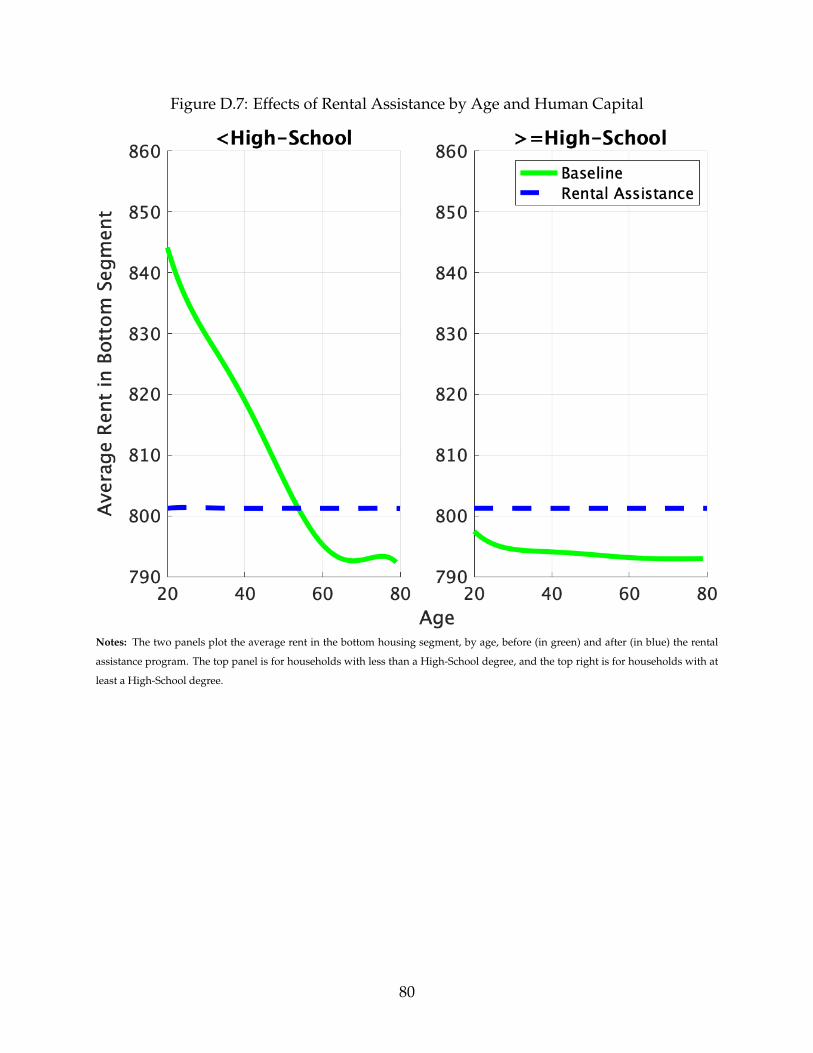
Figure D.7: Effects of Rental Assistance by Age and Human Capital

Notes: The two panels plot the average rent in the bottom housing segment, by age, before (in green) and after (in blue) the rental

assistance program. The top panel is for households with less than a High-School degree, and the top right is for households with at

least a High-School degree.

80

Table D.1: Balance Between Matched and Non-matched Eviction Cases (to Infutor)

Variable Matched(1)

Non-Matched(2)

Difference(3)

A. Case CharacteristicsEvicted 0.96 0.96 0

(0.2) (0.19) (0.01)

Amount Paid ($) 2, 933 3, 343 −410(2, 817) (9, 737) (350)

Length (days) 33.1 32.5 0.6(18.84) (17.87) (0.53)

Number of Defendants 2.34 2.25 0.09∗

(1.49) (1.48) (0.04)

3-day Notice 0.98 0.98 0(0.13) (0.13) (0.003)

B. Neighborhood CharacteristicsRent Burden 34.93 35.23 −0.3

(5.67) (5.95) (0.16)

Household Income ($) 54, 727 52, 841 1, 886∗

(21, 487) (21, 319) (568)

Monthly Rent ($) 1, 229 1, 210 19∗

(300) (293) (7.88)

Poverty Rate (%) 17.74 19.20 −1.46∗

(10.96) (11.52) (0.3)

Property Value ($) 373, 971 378, 452 −4, 481(160, 730) (163, 766) (4, 329)

Share African American (%) 6.48 6.82 −0.34(6.87) (6.87) (0.18)

Number of observations 2, 201 3, 941

Notes: This table reports the differences in case characteristics (Panel A) and neighborhood level characteristics (Panel B) between

eviction cases that are matched to Infutor data and cases that are not matched. For each case, neighborhood level characteristics

correspond to the mean at the tract level from the 2010-14 ACS. Column (1) reports the mean outcome for matched cases, column (2)

reports the mean outcome for non-matched cases, and column (3) reports the difference. Standard errors are in parenthesis. The

standard errors of the differences are computed based on a t-test. (*) means the the difference is significant at the 5% level. “Evicted”

is a dummy variable equal to one if the case ended with an eviction, “Amount Paid” is the dollar amount the tenants were ordered to

pay, “Length” is the number of days between case filing and case resolution, “Number of Defendants” is the number of individuals

appearing as defendants on the case, and “3-day notice” is a dummy equal to one if the notice period given to the tenant was 3 days

(instead of a 30 day notice which is given when the landlord seeks to evict a tenant who is on a month-by-month lease and who has

not violated the terms of the lease).

81

Table D.2: Rent Burden Across MSAs

MSA Median HouseholdIncome (Renters)

Median RentBurden

Standard Deviation(Rent Burden)

Greensboro-High Point $28,184 0.22 0.20Buffalo-Cheektowaga-Niagara Falls $28,847 0.22 0.22

Cleveland-Elyria $29,570 0.24 0.22Louisville/Jefferson $30,000 0.22 0.20

Pittsburgh $30,000 0.22 0.22Syracuse $30,000 0.24 0.22

Fresno, CA $30,843 0.28 0.24Cincinnati $31,495 0.22 0.22

Detroit-Warren-Dearborn $31,600 0.24 0.24Tucson $32,000 0.26 0.20

New Orleans-Metairie $32,052 0.26 0.24Milwaukee-Waukesha-West Allis $32,052 0.24 0.22

Grand Rapids-Wyoming $32,581 0.24 0.22Indianapolis-Carmel-Anderson $32,581 0.24 0.20

Bakersfield $33,000 0.26 0.22St. Louis $33,700 0.22 0.20

Columbus $35,000 0.22 0.20Nashville-Davidson–Murfreesboro $35,000 0.22 0.20

Charlotte-Concord-Gastonia $35,000 0.22 0.20Tampa-St. Petersburg-Clearwater $35,600 0.26 0.22

Kansas City $35,871 0.22 0.20San Antonio-New Braunfels $36,000 0.22 0.20

Jacksonville $36,250 0.24 0.20Albany-Schenectady-Troy $36,325 0.24 0.22

Orlando-Kissimmee-Sanford $36,800 0.28 0.22Miami-Fort Lauderdale-West Palm Beach $36,900 0.30 0.24

Philadelphia-Camden-Wilmington $37,600 0.26 0.22Atlanta-Sandy Springs-Roswell $37,921 0.24 0.22

Minneapolis-St. Paul-Bloomington $38,400 0.26 0.22Phoenix-Mesa-Scottsdale $39,206 0.24 0.20

Houston-The Woodlands-Sugar Land $39,314 0.22 0.20Riverside-San Bernardino-Ontario $40,000 0.28 0.22

Portland-Vancouver-Hillsboro $40,000 0.24 0.22Salt Lake City $40,000 0.24 0.20

Denver-Aurora-Lakewood $40,000 0.26 0.22Dallas-Fort Worth-Arlington $40,000 0.22 0.20

Chicago-Naperville-Elgin $40,000 0.24 0.22Sacramento–Roseville–Arden-Arcade $40,000 0.28 0.22

Las Vegas-Henderson-Paradise $42,000 0.24 0.20Austin-Round Rock $42,100 0.24 0.20

Baltimore-Columbia-Towson $45,000 0.24 0.22Los Angeles-Long Beach-Anaheim $45,500 0.30 0.24

New York-Newark-Jersey City $46,700 0.26 0.24Boston-Cambridge-Newton $47,200 0.26 0.22

Seattle-Tacoma-Bellevue $47,643 0.24 0.22San Diego-Carlsbad $47,864 0.30 0.22

San Francisco-Oakland-Hayward $58,000 0.26 0.22Washington-Arlington-Alexandria $61,493 0.26 0.20

San Jose-Sunnyvale-Santa Clara $68,000 0.26 0.22

Average $38,392 0.25 0.22Standard Deviation $8,166 0.02 0.01

Notes: This table reports the median household income of renters, the median rent burden, and the standard deviation of rent burden,

for each of the largest 50 MSAs in terms of population, using the 2010-14 ACS.

82