the west africa-america chamber of commerce & industries presents: big data & machine...
TRANSCRIPT

Combine historical track issue data and historical high resolution meteorological data with machine learning.
Combine Multiple Datasets

WaterThe Motive
Do well with the Details by embracing the Big Picture
Prof. David Lary+1 (972) 489-2059
http://[email protected]
Center for Space Science

Drought Has Increased Globally Since 1900

Worst Drought in 1,000 Years Predicted for American West
A paddle wheeler and a small motorboat sail on Lake Mead, North America's largest man-made reservoir. The water is at its lowest level since the Hoover Dam was built in the 1930s. The white "bathtub ring" of mineral deposits on the rocks marks past water levels.
PUBLISHED FEBRUARY 12, 2015

Western U.S. Drought Prompts Disaster Declarations In 11 States By MICHELLE RINDELS 01/16/14 07:51 PM ET EST
LAS VEGAS (AP) — Federal officials have designated portions of 11 drought-ridden western and central states as primary natural disaster areas, highlighting the financial strain the lack of rain is likely to bring to farmers in those regions.
The announcement by the U.S. Department of Agriculture on Wednesday included counties in Colorado, New Mexico, Nevada, Kansas, Texas, Utah, Arkansas, Hawaii, Idaho, Oklahoma and California.
Rancher Ralph Miller, 79, checks on one of many “stock tanks” of water that are receding due to the severe drought. “I’d say it’s just about as bad as it can get.”
Barnhart, Texas

“Water is the new oil”Jim Rogers, chief executive of Duke Energy... and many others
Water crisis in California, Texas threatens US food security Western water scarcity issues becoming more severe Western Farm Press, Jun. 5, 2012 University of Texas at Austin
California and Texas produced agricultural products worth $56 billion in 2007, accounting for much of the nation's food production. They also account for half of all groundwater depletion in the U.S., mainly as a result of irrigating crops.
The nation’s food supply may be vulnerable to rapid groundwater depletion from irrigated agriculture, according to a new study by researchers at The University of Texas at Austin and elsewhere.
http://westernfarmpress.com/irrigation/water-crisis-california-texas-threatens-us-food-security

Since 1980 the population of Texas has more than doubled, but the reservoir capacity has remained almost unchanged.
During 2011the reservoir levels were the lowest during Sep-Dec that they have been since 1990.
In 2015 we are starting out with lower levels than 2013.

Smarter irrigation control is invaluable!
If we can use existing infrastructure it is even better!
.... from farm, to corporate campus, to golf course, to your back yard.

When great societal need meets appropriate scalable solution
there is much societal and economic benefit to be
gained

How?
California Children Example

DATE: 12-Feb-2010
DOC NO: 0115056
ISSUE: 02
DMC DATA PRODUCT MANUAL
STATUS: FINAL
Page 16 of 127
Figure 4: Detector and channel layout of the SLIM-6-22 imager
Imager Bank 0
Channel 6 Green
Channel 5 Red
Channel 4 NIR
Imager Bank 1
Channel 1 NIR
Channel 2 Red
Channel 3 Green
Pixel 1
Pixel 14436
Pixel 14436
Pixel 1


uneven irrigation
blown valves lead to flooding
Sports fields
agricultural test plots
22 m resolution

On average, systems have water losses of about 17 percent.
49

Can you tell which grass has had more water?
Zooming in

Neighborhood
Trees
‘green’ pond
golf course
gated community
dry grass
Trees
Trees
Sports Field
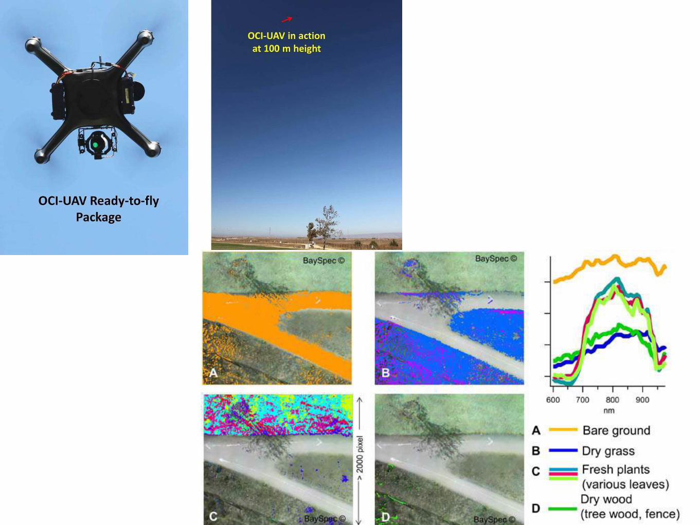

20 lb Airborne hyperspectral imaging system385 channels between 400-1,700 nm
Hyperspectral data cube

J S Famiglietti, and M Rodell Science 2013;340:1300-1301
www.sciencemag.org SCIENCE VOL 340 14 JUNE 2013 1301
PERSPECTIVES
an accuracy of 1.5 cm equivalent water height.Because GRACE measures changes in
total water storage, it integrates the impacts of natural climate fl uctuations, global change, and human water use, including groundwater extraction, which in many parts of the world is unmeasured and unmanaged. GRACE-derived rates of groundwater losses in the world’s major aquifer systems ( 4– 6) under-score the critical need to improve monitor-ing and regulation of groundwater systems before they run dry.
Regional fl ooding and drought are driven by the surplus or defi cit of water in a river basin or an aquifer, yet few hydrologic observing networks yield suffi cient data for comprehensive monitoring of changes in the total amount of water stored in a region. GRACE observations have helped to fill this gap. They have been used to character-ize regional fl ood potential ( 8) and to assess water storage deficits in the U.S. Drought Monitor ( 9) and are included in annual State of the Climate reports ( 10). As an integrated measure of all surface and groundwater stor-age changes, GRACE data implicitly contain a record of seasonal to interannual water stor-age variations that can likely be exploited to lengthen early warning periods for regional fl ood and drought prediction (see the fi gure).
The lack of comprehensive measurements also makes large-scale hydrological models,
key tools for predicting future water avail-ability, diffi cult to validate. Low-resolution GRACE data, when combined with higher-resolution model simulations, provide an independent constraint on simulated water balances, while also adding spatial detail to GRACE’s low-resolution perspective ( 11). They are widely used to evaluate land surface models used by weather and climate forecast-ing centers around the world ( 12).
Evapotranspiration is a key factor in interbasin water allocations, yet because it disperses into the atmosphere in the vapor phase, it confounds standard measurement techniques. The ability of GRACE to weigh changes in water stored in an entire river basin allows evapotranspiration to be esti-mated in a water balance framework ( 13).
Transboundary water availability issues require sharing hydrologic data across politi-cal boundaries. However, national hydrolog-ical records are often withheld for political, socioeconomic, and defense purposes, com-plicating regional water management discus-sions. Several studies have used GRACE data to circumvent international data denial prac-tices, including in those involving lakes ( 14), river basins ( 6), and aquifers ( 4, 6). Likewise, regional and global maps of emerging trends in water availability (see the figure) can underpin discussions of geopolitical water security, confl ict, and water diplomacy ( 6).
Although it still collects 10 months of data per year, GRACE has long outlived its planned 5-year life span. The GRACE Fol-low-On (GRACE-FO) mission, planned for launch in 2017, should enable continued col-lection of critical water and related climate observations for at least a decade, forestalling potential data gaps before a more advanced satellite gravimetry system is developed and launched, as tentatively planned for the 2020s.
For GRACE and its successors to maxi-mize their value for water management, key issues must be addressed. First, the current 2- to 6-month latency before GRACE data are released must be substantially reduced to enable their use in seasonal prediction. Sec-ond, GRACE data should be better integrated into the modeling and decision support sys-tems used by operational water management centers. Finally, next-generation missions beyond GRACE-FO should aim to achieve higher spatial (<50,000 km2) and temporal (weekly or biweekly) resolution, for exam-ple through novel orbital confi gurations, so that smaller river basins and aquifers can be observed directly. The availability of GRACE data at these fi ner scales, at which most plan-ning decisions are made, would likely ensure their broader use in water management.
The GRACE-FO mission is on sched-ule for a 2017 launch, but a next-generation, improved GRACE mission is still under design and as yet unconfirmed. Given its demonstrated contributions to date and the potential for much more, a future without a GRACE mission in orbit would be an unfor-tunate and unnecessarily risky backward step for regional water management.
References
1. P. J. Durack et al., Science 336, 455 (2012). 2. K. E. Trenberth, Clim. Res. 47, 123 (2011). 3. I. M. Held, B. J. Soden, J. Clim. 19, 5686 (2006). 4. V. M. Tiwari, J. Wahr, S. Swenson, Geophys. Res. Lett. 36,
L18401 (2009). 5. B. R. Scanlon et al., Proc. Natl. Acad. Sci. U.S.A. 109,
9320 (2012). 6. K. A. Voss et al., Water Resour. Res. 49, 904 (2013). 7. B. D. Tapley et al., Science 305, 503 (2004). 8. J. T. Reager, J. S. Famiglietti, Geophys. Res. Lett. 36,
L23402 (2009). 9. R. Houborg et al., Water Resour. Res. 48, W07525 (2012). 10. J. Blunden, D. S. Arndt, Eds., Bull. Am. Meteorol. Soc. 93,
S1 (2012). 11. B. F. Zaitchik et al., J. Hydrometeorol. 9, 535 (2008). 12. S. C. Swenson, P. C. D. Milly, Water Resour. Res. 42,
W03201 (2006). 13. G. Ramillien et al., Water Resour. Res. 42, W10403 (2006). 14. S. Swenson, J. Wahr, J. Hydrol. 370, 163 (2009). 15. J. S. Famiglietti, Abstract GC31D-01, fall meeting, AGU,
San Francisco, 3 to 7 December 2012.
Supplementary Materials www.sciencemag.org/cgi/content/full/science.1236460/DC1 Fig. S1
CR
ED
IT: C
AR
OLIN
E D
E L
INA
GE
/UN
IV. O
F C
ALIF
OR
NIA
, IR
VIN
E
50°N
40°N
30°N
70°W
80°W
90°W100°W110°W
120°W
–3 –2 –1 0 1 2 3
H2O (cm/year)
15
2 3
4
6
Mixed picture. Between 2003 and 2012, GRACE data show water losses in agricultural regions such as Cali-fornia’s Central Valley (1) (�1.5 ± 0.1 cm/year) and the Southern High Plains Aquifer (2) (�2.5 ± 0.2 cm/year), caused by overreliance on groundwater to supply irrigation water. Regions where groundwater is being depleted as a result of prolonged drought include Houston (3) (�2.3 ± 0.6 cm/year), Alabama (4) (�2.1 ± 0.8 cm/year), and the Mid-Atlantic states (5) (�1.8 ± 0.6 cm/year). Water storage is increasing in the fl ood-prone Upper Missouri River basin (6) (2.5 ± 0.2 cm/year). See fi g. S1 for monthly time series for all hot spots. Data from ( 15) and from GRACE data release CSR RL05.
10.1126/science.1236460
Published by AAAS
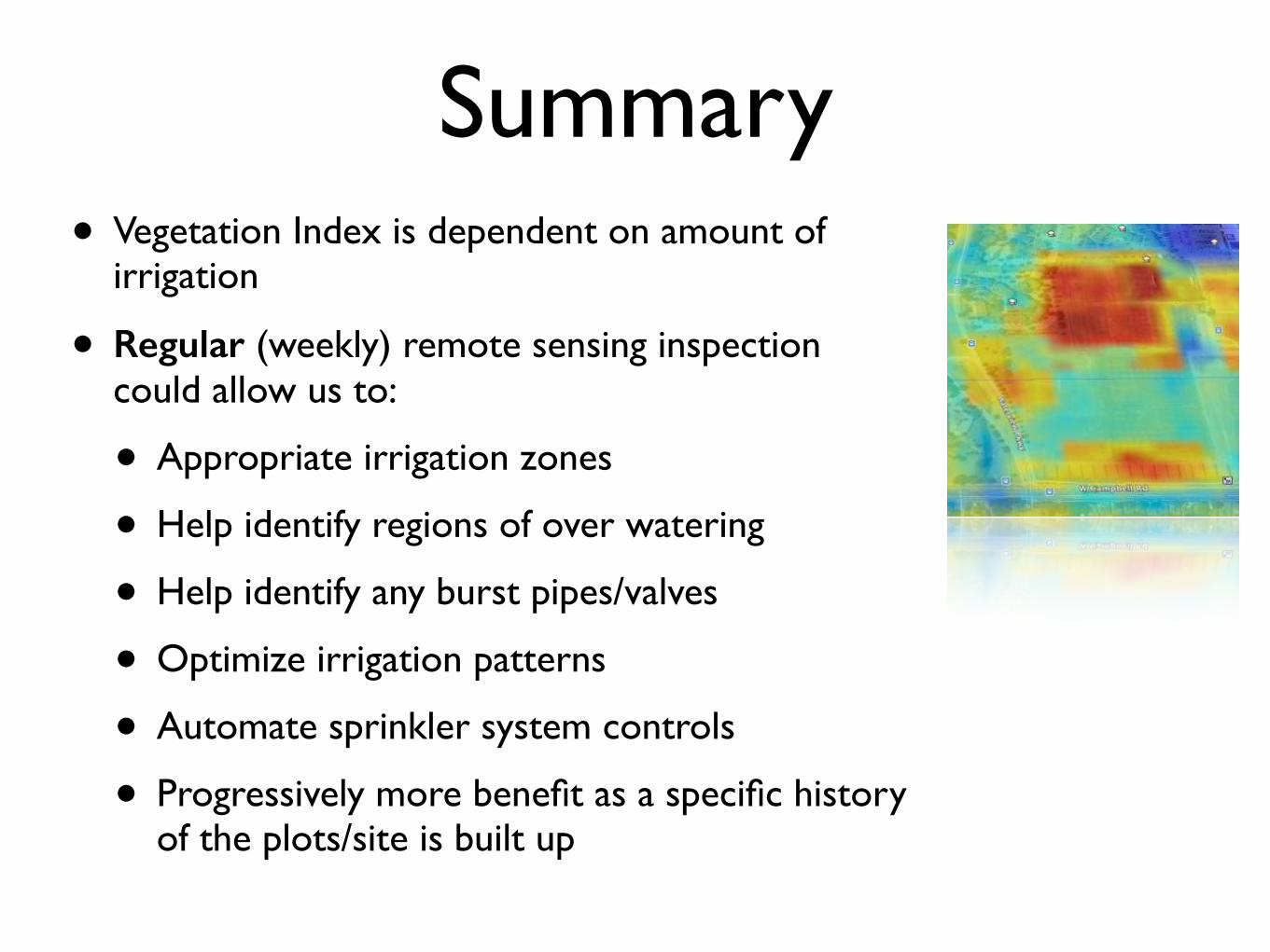
Summary• Vegetation Index is dependent on amount of
irrigation
• Regular (weekly) remote sensing inspection could allow us to:
• Appropriate irrigation zones
• Help identify regions of over watering
• Help identify any burst pipes/valves
• Optimize irrigation patterns
• Automate sprinkler system controls
• Progressively more benefit as a specific history of the plots/site is built up

Stage 2

FUTURE Water Management
Why Agriculture? ~80% water use US (USDA 2013)
Challenges: Climate change, Drought, Population, non-ag water uses.
Water Use Efficiency: ~50% US (USDA 2004)
Water Mgmt. “Smart-GRID*”
Delivery
Models
Basin Geodata
Water/Crop Status & Forecast
Water Need Status & Forecast
Water Agric +Others
Status & Forecast

Current Water Mgmt.
Delivery
Models
Basin Geodata
Water/Crop Status & Forecast
Water Status & Forecast
Water Agric +Others
Status & Forecast
Water use based on:
Experience Limited estimations
No related info
CURRENT Water Management

CWMIS Case Example: Water Use vs. Delivery
TOP: crop water use vs. water delivery (ac-ft). BOTTOM: water use difference (ac-ft)
Typically save at least 10% Can be done on a field by field, campus by campus, home by home, or golf course by golf course basis or for an entire basin.
Alfonso Torres


Culex tarsalis
West Nile Virus
The same data infrastructure can also be used to help combat West Nile Virus by identifying breeding sites.

Malaria Prediction Using Satellite Data

P. vivax is carried by the female Anopheles mosquito

Plasmodium vivax is a protozoal parasite and a human pathogen. The most frequent and widely distributed cause of recurring (Benign tertian) malaria, P. vivax is one of the six species of malaria parasites that commonly infect humans.[1] It is less virulent than Plasmodium falciparum, the deadliest of the six, but vivax malaria can lead to severe disease and death.[2][3] P. vivax is carried by the female Anopheles mosquito, since it is only the female of the species that bite.
Plasmodium vivax
Plasmodium falciparum http://www.worldmalariareport.org/

Seasonal climatic suitability for malaria transmission (CSMT)Climatic conditions are considered to be suitable for transmission when the monthly precipitation accumulation is at least 80 mm, the monthly mean temperature is between 18°C and 32°C and the monthly relative humidity is at least 60%. These thresholds are based on a consensus of the literature. In practice, the optimal and limiting conditions for transmission are dependent on the particular species of the parasite and vector.
Commentary: Web-based climate information resources for malaria control in Africa Emily K Grover-Kopec, M Benno Blumenthal, Pietro Ceccato, Tufa Dinku, Judy A Omumbo and Stephen J Connor* Malaria Journal 2006, 5:38 doi:10.1186/1475-2875-5-38


0 500 1,000 Km
Map Produced by USGS/EROS
Vectorial CapacityIn Zones with Malaria Epidemic Potential
05 August - 12 August 2013
VCAP Values
00 - 22 - 44 - 66 - 88 - 1010 - 1515 - 20> 20
Country Boundaries

Satellite imagery can be used to track mosquito habitats.
High-resolution (5 m) satellite images can identify very small water bodies, wetlands and other malaria-relevant land-cover types.
Of the 225 million annual reported cases of the disease, 212 million of these occur in Africa. Of the 800,000 Malaria-related deaths each year, 90% of these fatalities occur in sub-Saharan Africa.
http://www.itweb.co.za/index.php?option=com_content&view=article&id=52695

T H R I V E T I M E LY HE A LT H I N D I C AT O R S U S I N G RE M O T E S E N S I N G & IN N O VAT I O N F O R T H E V I TA L I T Y O F T H E EN V I R O N M E N T
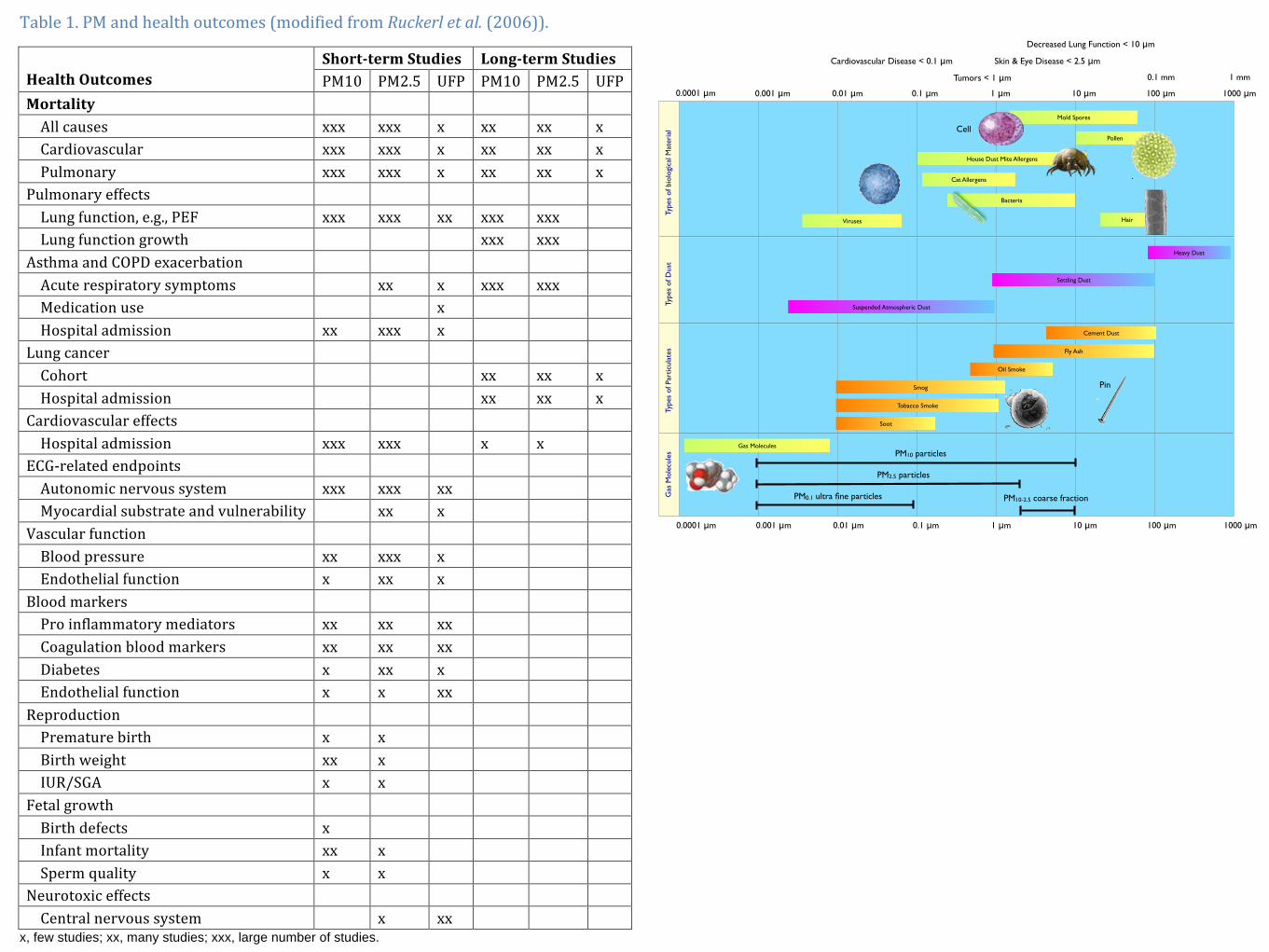
Why we care so much? Approximately 50 million Americans have allergic diseases, including asthma and allergic rhinitis, both of which can be exacerbated by PM2.5.
Every day in America 44,000 people have an asthma attack, and because of asthma 36,000 kids miss school, 27,000 adults miss work, 4,700 people visit the emergency room, 1,200 people are admitted to the hospital, and 9 people die.

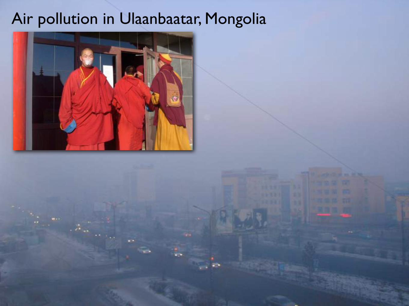
Air pollution in Ulaanbaatar, Mongolia

Unprecedented levels of air pollution in Singapore and Malaysia in June led to respiratory illnesses, school closings, and grounded aircraft. This year it was so bad that in some affected areas there was a 100 percent rise in the number of asthma cases, and the government of Malaysia distributed gas masks.
MODIS Aqua July 21, 2013.
David Lary
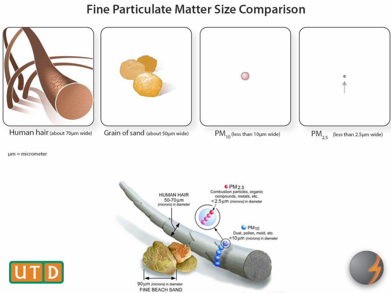

PM2.5 Invisible Killer

Type
s of
bio
logi
cal M
ater
ial
Type
s of
Dus
tTy
pes
of P
artic
ulat
esG
as M
olec
ules
0.0001 μm 0.001 μm 0.01 μm 0.1 μm 1 μm 10 μm 100 μm 1000 μm
Pollen
Mold Spores
House Dust Mite Allergens
Bacteria
Cat Allergens
Viruses
Heavy Dust
Settling Dust
Suspended Atmospheric Dust
Cement Dust
Fly Ash
Oil Smoke
Smog
Tobacco Smoke
Soot
Gas Molecules
Decreased Lung Function < 10 μm
Skin & Eye Disease < 2.5 μm
Tumors < 1 μm
Cardiovascular Disease < 0.1 μm
Hair
Pin
Cell
0.0001 μm 0.001 μm 0.01 μm 0.1 μm 1 μm 10 μm 100 μm 1000 μm
PM10 particles
PM2.5 particles
PM0.1 ultra fine particles PM10-2.5 coarse fraction
0.1 mm 1 mm
! 5!
Table!1.!PM!and!health!outcomes!(modified!from!Ruckerl*et*al.!(2006)).!
!!Health*Outcomes!
Short9term*Studies* Long9term*Studies*PM10! PM2.5! UFP! PM10! PM2.5! UFP!
Mortality* !! !! !! !! !! !!
!!!!All!causes! xxx!! xxx!! x! xx! xx! x!!!!!Cardiovascular! xxx! xxx! x!! xx! xx! x!
!!!!Pulmonary! xxx! xxx! x! xx! xx! x!Pulmonary!effects! !! !! !! !! !! !!
!!!!Lung!function,!e.g.,!PEF! xxx! xxx! xx! xxx! xxx! !!!!!!Lung!function!growth! !! !! !! xxx! xxx! !!
Asthma!and!COPD!exacerbation! !! !! !! !! !! !!
!!!!Acute!respiratory!symptoms! !! xx! x! xxx! xxx! !!!!!!Medication!use! !! !! x! !! !! !!
!!!!Hospital!admission! xx! xxx! x! !! !! !!Lung!cancer! !! !! !! !! !! !!
!!!!Cohort! !! !! !! xx! xx! x!
!!!!Hospital!admission! !! !! !! xx! xx! x!Cardiovascular!effects! !! !! !! !! !! !!
!!!!Hospital!admission! xxx! xxx! !! x! x! !!ECG@related!endpoints! !! !! !! !! !! !!
!!!!Autonomic!nervous!system! xxx! xxx! xx! !! !! !!!!!!Myocardial!substrate!and!vulnerability! !! xx! x! !! !! !!
Vascular!function! !! !! !! !! !! !!
!!!!Blood!pressure! xx! xxx! x! !! !! !!!!!!Endothelial!function! x! xx! x! !! !! !!
Blood!markers! !! !! !! !! !! !!!!!!Pro!inflammatory!mediators! xx! xx! xx! !! !! !!
!!!!Coagulation!blood!markers! xx! xx! xx! !! !! !!
!!!!Diabetes! x! xx! x! !! !! !!!!!!Endothelial!function! x! x! xx! !! !! !!
Reproduction! !! !! !! !! !! !!!!!!Premature!birth! x! x! !! !! !! !!
!!!!Birth!weight! xx! x! !! !! !! !!!!!!IUR/SGA! x! x! !! !! !! !!
Fetal!growth! !! !! !! !! !! !!
!!!!Birth!defects! x! !! !! !! !! !!!!!!Infant!mortality! xx! x! !! !! !! !!
!!!!Sperm!quality! x! x! !! !! !! !!Neurotoxic!effects! !! !! !! !! !! !!
!!!!Central!nervous!system!! !! x! xx! !! !! !!x, few studies; xx, many studies; xxx, large number of studies.

Hourly Measurements from 55 countries and more than 8,000 measurement sites from 1997-present
REMOTE SENSING, MACHINE LEARNING AND PM2.5 4
Random Forests, etc.) that can provide multi-variate non-linearnon-parametric regression or classification based on a trainingdataset. We have tried all of these approaches for estimatingPM2.5 and found the best by far to be Random Forests.
B. Random ForestsIn this paper we use one of the most accurate machine learn-
ing approaches currently available, namely Random Forests[53], [54]. Random forests are composed of an ensemble ofdecision trees [55]. Random forests have many advantagesincluding their ability to work efficiently with large datasets,accommodate thousands of input variables, provide a measureof the relative importance of the input variables in the re-gression, and effectively handling datasets containing missingdata.
Each tree in the random forest is a decision tree. A decisiontree is a tree-like graph that can be used for classificationor regression. Given a training dataset, a decision tree canbe grown to predict the value of a particular output variablebased on a set of input variables [55]. The performanceof the decision tree regression can be improved upon if,instead of using a single decision tree, we use an ensembleof independent trees, namely, a random forest [53], [54]. Thisapproach is referred to as tree bootstrap aggregation, or treebagging for short.
Bootstrapping is a simple way to assign a measure of ac-curacy to a sample estimate or a distribution. This is achievedby repeatedly randomly resampling the original dataset toprovide an ensemble of independently resampled datasets.Each member of the ensemble of independently resampleddatasets is then used to grow an independent decision tree.
The statistics of random sampling means that any given treeis trained on approximately 66% of the training dataset andso approximately 33% of the training dataset is not used intraining any given tree. Which 66% is used is different foreach of the trees in the random forest. This is a very rigorousindependent sampling strategy that helps minimize over fittingof the training dataset (e.g. learning the noise). In addition, inour implementation we keep back a random sample of data notused in the training for independent validation and uncertaintyestimation.
The members of the original training dataset not used in agiven bootstrap resample are referred to as out of bag forthis tree. The final regression estimate that is provided bythe random forest is simply the average of the ensemble ofindividual predictions in the random forest.
A further advantage of decision trees is that they can provideus the relative importance of each of the inputs in constructingthe final multi-variate non-linear non-parametric regressionmodel (e.g. Tables II and III).
C. Datasets Used in Machine Learning Regression1) PM2.5 Data: As many hourly PM2.5 observations
as possible that were available from the launch of Terraand Aqua to the present were used in this study. Forthe United States this data came from the EPA AirQuality System (AQS) http://www.epa.gov/ttn/airs/airsaqs/
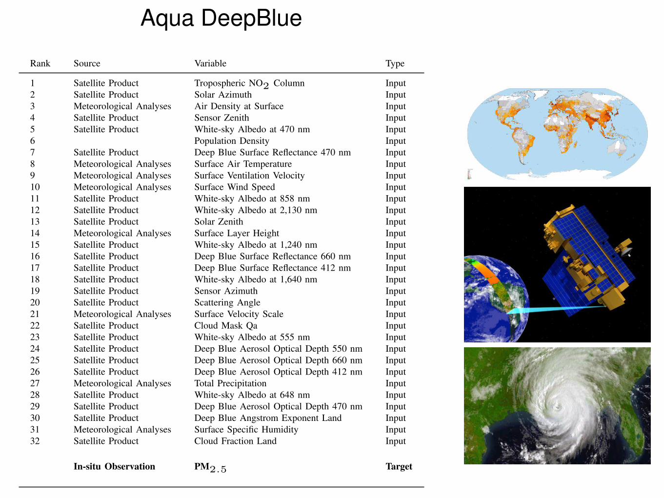
TABLE IIVARIABLES USED IN THE MACHINE LEARNING ESTIMATE OF PM2.5 FORTHE MODIS COLLECTION 5.1 PRODUCTS FOR THE TERRA AND AQUADEEP BLUE ALGORITHM SORTED BY THEIR IMPORTANCE. THE MOST
IMPORTANCE VARIABLE FOR A GIVEN REGRESSION IS PLACED FIRST WITHA RANK OF 1.
Terra DeepBlue
Rank Source Variable Type
1 Population Density Input2 Satellite Product Tropospheric NO2 Column Input3 Meteorological Analyses Surface Specific Humidity Input4 Satellite Product Solar Azimuth Input5 Meteorological Analyses Surface Wind Speed Input6 Satellite Product White-sky Albedo at 2,130 nm Input7 Satellite Product White-sky Albedo at 555 nm Input8 Meteorological Analyses Surface Air Temperature Input9 Meteorological Analyses Surface Layer Height Input10 Meteorological Analyses Surface Ventilation Velocity Input11 Meteorological Analyses Total Precipitation Input12 Satellite Product Solar Zenith Input13 Meteorological Analyses Air Density at Surface Input14 Satellite Product Cloud Mask Qa Input15 Satellite Product Deep Blue Aerosol Optical Depth 470 nm Input16 Satellite Product Sensor Zenith Input17 Satellite Product White-sky Albedo at 858 nm Input18 Meteorological Analyses Surface Velocity Scale Input19 Satellite Product White-sky Albedo at 470 nm Input20 Satellite Product Deep Blue Angstrom Exponent Land Input21 Satellite Product White-sky Albedo at 1,240 nm Input22 Satellite Product Scattering Angle Input23 Satellite Product Sensor Azimuth Input24 Satellite Product Deep Blue Surface Reflectance 412 nm Input25 Satellite Product White-sky Albedo at 1,640 nm Input26 Satellite Product Deep Blue Aerosol Optical Depth 660 nm Input27 Satellite Product White-sky Albedo at 648 nm Input28 Satellite Product Deep Blue Surface Reflectance 660 nm Input29 Satellite Product Cloud Fraction Land Input30 Satellite Product Deep Blue Surface Reflectance 470 nm Input31 Satellite Product Deep Blue Aerosol Optical Depth 550 nm Input32 Satellite Product Deep Blue Aerosol Optical Depth 412 nm Input
In-situ Observation PM2.5 Target
Aqua DeepBlue
Rank Source Variable Type
1 Satellite Product Tropospheric NO2 Column Input2 Satellite Product Solar Azimuth Input3 Meteorological Analyses Air Density at Surface Input4 Satellite Product Sensor Zenith Input5 Satellite Product White-sky Albedo at 470 nm Input6 Population Density Input7 Satellite Product Deep Blue Surface Reflectance 470 nm Input8 Meteorological Analyses Surface Air Temperature Input9 Meteorological Analyses Surface Ventilation Velocity Input10 Meteorological Analyses Surface Wind Speed Input11 Satellite Product White-sky Albedo at 858 nm Input12 Satellite Product White-sky Albedo at 2,130 nm Input13 Satellite Product Solar Zenith Input14 Meteorological Analyses Surface Layer Height Input15 Satellite Product White-sky Albedo at 1,240 nm Input16 Satellite Product Deep Blue Surface Reflectance 660 nm Input17 Satellite Product Deep Blue Surface Reflectance 412 nm Input18 Satellite Product White-sky Albedo at 1,640 nm Input19 Satellite Product Sensor Azimuth Input20 Satellite Product Scattering Angle Input21 Meteorological Analyses Surface Velocity Scale Input22 Satellite Product Cloud Mask Qa Input23 Satellite Product White-sky Albedo at 555 nm Input24 Satellite Product Deep Blue Aerosol Optical Depth 550 nm Input25 Satellite Product Deep Blue Aerosol Optical Depth 660 nm Input26 Satellite Product Deep Blue Aerosol Optical Depth 412 nm Input27 Meteorological Analyses Total Precipitation Input28 Satellite Product White-sky Albedo at 648 nm Input29 Satellite Product Deep Blue Aerosol Optical Depth 470 nm Input30 Satellite Product Deep Blue Angstrom Exponent Land Input31 Meteorological Analyses Surface Specific Humidity Input32 Satellite Product Cloud Fraction Land Input
In-situ Observation PM2.5 Target
detaildata/downloadaqsdata.htm and AirNOW http://www.airnow.gov. In Canada the data came from http://www.etc-cte.ec.gc.ca/napsdata/main.aspx. In Europe the data camefrom AirBase, the European air quality database main-tained by the European Environment Agency and the Euro-

This is a BigData Problem of Great Societal Relevance
• Collecting data in real time from national and global networks requires bandwidth.
• With the next generation of wearable sensors and the internet of things this data volume will rapidly increase.
• A variety of applications enabled by BigData, higher bandwidth and cloud processing.
• Future finer granularity and two way communication will dramatically increase the size of the data bringing air quality to the micro scale, just like weather data.
Time Taken10 Mbps 20 Mbps 50 Mbps 1 Gbps
40 TB training data4 Gb update
185 days 93 days 37 days 1 day 21 hours54m 27m 11m 32s

Long-Term Average 1997-present
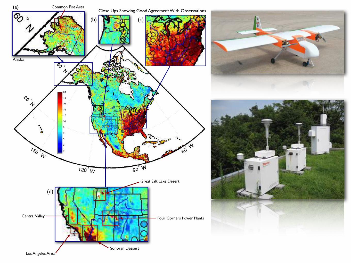
Four Corners Power Plants
Sonoran DessertLos Angeles Area
Central Valley
Common Fire AreaClose Ups Showing Good Agreement With Observations
Alaska
(a)
(b) (c)
(d)
Great Salt Lake Desert

Automated traffic patterns, driverless cars routing
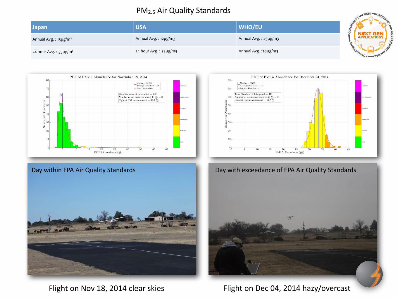
Flight on Nov 18, 2014 clear skies Flight on Dec 04, 2014 hazy/overcast
Japan USA WHO/EU
Annual Avg. : 15μg/m3 Annual Avg. : 12μg/m3 Annual Avg. : 25μg/m3
24 hour Avg. : 35μg/m3 24 hour Avg. : 35μg/m3 Annual Avg. :20μg/m3
PM2.5 Air Quality Standards
Day within EPA Air Quality Standards Day with exceedance of EPA Air Quality Standards

50

Model Airplane Details
A 12s 5400 mAh baLery pack per motor (current setup) provides approximately 8 minutes of flight Pme. Flight Pme can be increased by using higher capacity baLery packs.

Flight Photos

AccomplishmentsTo the best of our knowledge the first time the full sub-pixel aerosol size distribution has been characterized at high spatial resolution (sub meter) and high temporal resolution (every second) using:
• A zero emission, low cost, electric remote control model aircraft at multiple vertical levels in the lower most 100 m of the atmosphere.
• A car driving daily across a 10 km pixel over an extended period.
Satellite Pixel
Full Aerosol Size Distribution

G E O L O C AT E D A L L E R G E N S E N S I N G P L AT F O R M
G A S PFour objectives:
1. Develop and deploy an array of Internet of Things remote airborne particle sensors within Chattanooga to be used to provide real-time streamed data on hourly particulate levels, both pollen- sized (10-40 micron) and smaller (<2.5 micron) particles.
2. Deploy an in-situ pollen air sampler in Chattanooga to identify specific pollen types.
3. Merge locally streamed data with already-collected, satellite-based NASA data to complement and enhance the newly-collected particulate data and generate Chattanooga-focused particulate maps.
4. Develop web-based visual tools to provide real-time pollen and smaller particle alerts to end users such as asthma patients, health institutions, and businesses and other institutions affected by elevated pollen levels.
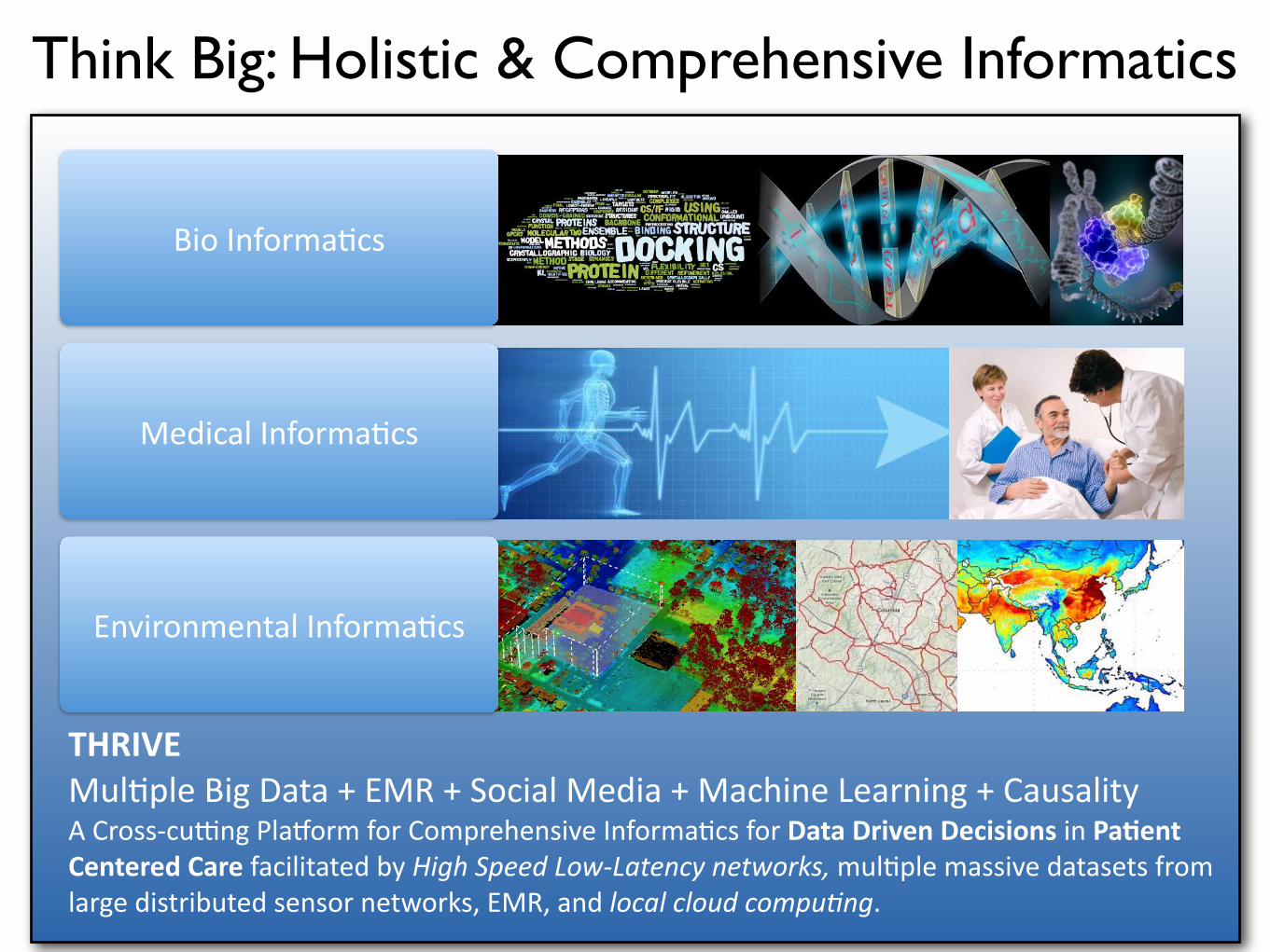
Think Big: Holistic & Comprehensive Informatics
Bio InformaPcs
Medical InformaPcs
Environmental InformaPcs
THRIVE MulPple Big Data + EMR + Social Media + Machine Learning + Causality A Cross-‐cuXng PlaYorm for Comprehensive InformaPcs for Data Driven Decisions in Pa<ent Centered Care facilitated by High Speed Low-‐Latency networks, mulPple massive datasets from large distributed sensor networks, EMR, and local cloud compu:ng.

Combine historical track issue data and historical high resolution meteorological data with machine learning.
Combine Multiple Datasets

Satellite Images can be used to automate the highlighting of vegetation near the tracks
Highlight Vegetation

1
Routine satellite acquisition of multispectral and SAR imagery
2
Periodic high resolution ground truth from aerial surveys
3
Image processing & Machine Learning
BNSF Decision Support
4
The synergy between routine satellite imagery, periodic high resolution ground truth surveys and automated machine learning and image processing is a powerful combination for decision support.
Preparing for Routine Decision Support