the weyburn co2 injection project

Chapter 2The Weyburn CO2 Injection Project

Canada is an interesting place, the rest of the world thinks so,even if Canadians don’t.

Terence M. Green

2.1 Introduction to Weyburn

A major issue concerning CCS is the lack of field demonstration. Plausible theo-ries have been developed to cover most aspects of this process. However, there are atpresent only four major operational examples where CO2 is injected for the purposesof storage: Statoil’s Sleipner and Snøhvit sites in the North Sea, BP’s In Salah Field(Algeria), and Weyburn. These pilot scale projects are intended to be used as exper-iments where ideas and theories relating to CO2 storage can be tested, and whereprinciples of best practise can be developed for future application to larger projects.Other projects likely to become operational in the near future are at the Gorgon Field(West Australia), and Shell’s QUEST (Alberta) and Barendrecht (The Netherlands)projects. The EU has mandated that 12 CCS demonstration projects come online by2015.

The Weyburn oil-field, located in central Canada, was selected as the location fora major research project into CCS by the Canadian Petroleum Technology ResearchCenter (PTRC) in collaboration with the field operators EnCana (now Cenovus)and the International Energy Agency (IEA). The aim was to develop a field scaledemonstration of CCS in order to verify the ability of an oil-field to store CO2. Theknowledge thus gained would be used as a guide for best practise when implementingCCS projects worldwide (Wilson et al. 2004). In July 2000 a storage component wasadded to EnCana’s Enhanced Oil Recovery (EOR) operation at the Weyburn-MidaleField. CO2 has been injected through an increasing number of patterns since 2000,and the current rate of injection is ∼3 million tonnes/year. It is anticipated that 50million tonnes will be stored during the life-of-field (LOF). This is equivalent to the

J. P. Verdon, Microseismic Monitoring and Geomechanical Modelling of CO2 Storage 11in Subsurface Reservoirs, Springer Theses, DOI: 10.1007/978-3-642-25388-1_2,© Springer-Verlag Berlin Heidelberg 2012

12 2 The Weyburn CO2 injection project

Fig. 2.1 Geographic location of the Weyburn field taken from Wilson et al. (2004). The field is setin the Williston sedimentary basin, which stretches across much of the north of the USA and centralCanada

emissions from 400,000 (gas-guzzling American) cars per year. The CO2 is deliveredto Weyburn through a pipeline from a coal gasification plant in Beulah, North Dakota.The primary form of monitoring is 4-D controlled source reflection seismology. Thechanges in the reflection amplitude of the reservoir layer have been used to imagethe spread of CO2 plumes from the injection wells (White 2008).

As part of the monitoring component of the project, geophones were installedin a disused borehole near to an injection site, with the aim of assessing the useof microseismic techniques for monitoring CO2 injection. In this chapter I outlinethe geological setting and history of Weyburn, before focusing on the microseismicevents recorded. The events have been located by contractors (ESG) and I discussthem here in relation to changes in injection and production in nearby wells.

2.2 Weyburn Geological Setting

The Weyburn field is situated in the Williston depositional basin, Saskatchewan,central Canada (Fig. 2.1). The basin contains shallow marine sediments depositedfrom the Cambrian through to the Mesozoic. Figure 2.2 shows some of the majorstratigraphic divisions identified in the basin. The Weyburn reservoir is found in theCharles Formation at depths of 1300–1500 m. These rocks were formed in a periti-dal regression-transgression sequence, depositing carbonates during high-stands andevaporitic dolomites during low-stands.

2.2 Weyburn Geological Setting 13

Fig. 2.2 Major stratigraphicgroups in the Williston Basintaken from Pendrigh (2004).The Weyburn reservoir is ofCarboniferous age, set in theCharles Formation, whichmakes up part of theMadison Group

The Weyburn reservoir is situated in the Midale carbonate cycle. The reservoir isusually split into two parts, a lower limestone layer, the Vuggy, and an upper dolostonelayer, the Marly. The Vuggy is so named because it contains vugs, or pore cavitieslarger than the grain size (as opposed to normal pores, which are usually smallerthan the grains). The Vuggy is usually split into two components—the shoal andintershoal members. Table 2.1 lists the lithological properties of the rocks that makeup the Weyburn reservoir. The seal for this reservoir group is the overlying MidaleEvaporite. This was formed during the last phase of regression during deposition ofthe Midale strata. It consists of low permeability nodular and laminated anhydrite of2–10 m thickness. This bed forms a band of low-permeability caprock across muchof Saskatchewan (Wilson et al. 2004). A second important seal is the MesozoicLower Watrous member, which lies unconformably on the Carboniferous beds. Thismember is of mixed lithology, but is generally siliclastic, and forms an impermeablelayer due to its clay content and diagenetic infilling of pores. Figure 2.3 shows aschematic diagram of the reservoir arrangement.

2.2.1 History of the Weyburn Field

It is estimated that the Weyburn reservoir initially held approximately1.4 billion barrels of oil. Production at Weyburn began in 1954, continuing until


Table 2.1 Lithological properties of the rocks of the Weyburn reservoir. Taken from Wilson et al.(2004)

Vuggy Shoal Vuggy Intershoal Marly

Lithology Coarse grainedcarbonate sand

Muddy carbonate Microsucrosic dolomite

Permeability range 10–500 mD 0.1–25 mD 1–100 mDAvg permeability 50 mD 3 mD 10 mDPorosity range 0.12–0.2 0.03–0.12 0.16–0.38Avg porosity 0.15 0.1 0.26Thickness 10–22 m 10–22 m 6–10 mSedimentary facies Marine lagoonal

carbonate shoalLow energy lagoonal

intershoalLow energy marine

Fig. 2.3 Schematic cross section of the Weyburn reservoir taken from Wilson et al. (2004). TheWeyburn reservoir is split into the lower intershoal and shoal Vuggy (V) and upper Marly (M) units.The primary seal is the Midale anhydrite, while an important secondary seal is the unconformablyoverlying Watrous member of Jurassic age

1964, when waterflood was initiated to increase production. Production peaked afterthe waterflood at 46,000 barrels/day, and has been decreasing since. In 1991 drillingof horizontal wells was initiated to increase production, targeting in particular theless permeable Marly layer. It is estimated that prior to CO2 injection, 25% of theoriginal oil in place had been recovered. In 2000, injection of CO2 was initiated, withthe intention of increasing oil production in the 19 patterns of Phase IA. The CO2 issourced from a coal gasification plant in North Dakota, and is transported througha pipeline to the field. CO2 is injected in horizontal wells while water continues tobe injected through vertical wells. Following the success of Phase IA, CO2 injectionhas been initiated in further patterns, Phase IB and Phase II, as well as the adjacentMidale Field. CO2 is injected at a rate of between 74–588 tonnes per day per well.Enhanced oil recovery associated with the CO2 injection currently accounts for 5,000barrels of the 20,000 barrels per day total production at Weyburn. It is estimated thatthe EOR operations will increase production by 130 million barrels (10% of theoriginal oil in place) and prolong the life of the field by 25 years.

2.2 Weyburn Geological Setting 15

When the Weyburn Field was discovered, pore pressure was estimated to be14 MPa. During production, this dropped to between 2 and 6 MPa. During water-flood, pressures increased to between 8 and 19 MPa. Pressures in the Phase IA areaare between 12.5–18 MPa (Brown 2002), with maximum anticipated pore pressureduring injection of 23–25 MPa.

A range of techniques have been deployed to monitor the initial CO2 flood in PhaseIA, including 4-D controlled source seismics, wellhead pressure sampling, cross welland vertical seismic profiling, geochemical analysis and soil gas sampling (Wilsonet al. 2004). However, microseismic monitoring was not used at this stage. The 4-Dseismic monitoring has been the most successful in imaging CO2 saturation (White2009), where travel time-shifts in the reservoir and reflection amplitude increasesat the top of the reservoir are used to image zones of CO2 saturation (Fig. 2.4).In Phase IA the 4-D seismics show the CO2 plumes migrating out from the horizontalinjection wells.

In 2003, downhole microseismic monitoring was initiated with a new CO2 injec-tion site. This stage, named Phase IB and located to the southeast of Phase IA,is the only place at Weyburn so far to use microseismic monitoring. The injection,production and monitoring wells of Phase IB are shown in Fig. 2.5.

2.3 Microseismic Monitoring at Weyburn

Microseismic monitoring seeks to detect the seismic emissions produced by frac-turing and fault reactivation around the reservoir. This technique was developed inthe early 1990s, and has been used increasingly since then. The magnitudes of suchevents are such that they cannot usually be detected at the surface, so geophones areplaced in boreholes near to the reservoir. When seismic energy is detected at the geo-phones, event location algorithms are used to locate the source of these emissions,indicating a point in the rock mass that has undergone brittle failure. Seismic energycan also be generated by other subsurface phenomena such as fluid motion throughpipes and conduits (e.g., Balmforth et al. 2005), although these processes are notthought to be occurring at Weyburn. It is anticipated that CO2 injection at Weyburnwill alter the pore pressure and stress fields at Weyburn enough to generate failure.By tracking the event locations, the operators hope to track the regions of failure,and thereby the stress changes, and also to assess whether the fracturing presents arisk to the security of storage.

2.3.1 System Setup

Phase IB has a vertical well (121/06-08) injecting CO2 at a rate of between50–250 MSCM/day (100–500 tonnes/day). To the northwest and to the southeastare horizontal producing wells (191/11-08, 192/09-06 and 191/10-08), all runningNE-SW. Wells 191/11-08 and 192/09-06 were both in production before the arraywas installed, while well 191/10-08 was drilled in July 2005, 18 months after


Fig. 2.4 Results from the 4-D controlled source seismic survey at Weyburn taken from (Li 2003).a shows the changes in reflection amplitude at the top of the reservoir, while b shows the travel time-shift through the reservoir. Changes in reflection amplitude and increases in travel-time through thereservoir image the CO2 plumes around the horizontal injection wells

CO2 injection had begun. The injection well was completed in November 2003,with water injection beginning on December 15th. CO2 injection began on the21st January. In August 2003 an 8-level, 3-component geophone string was installedin a disused vertical production well (101/06-08) about 50 m to the east of the injec-tion well. The sensors were sited at the depths given in Table 2.2. The top of the

2.3 Microseismic Monitoring at Weyburn 17

Fig. 2.5 Map view of themicroseismic setup atWeyburn. The verticalinjection and monitoringwells are located within 50 mof each other. To the NE andthe SW are horizontal oilproduction wells. Well191/10-08 began productionin July 2005, after Phase IBbut before Phase II

500 0 500 500

0

500

Easting (m)

Nor

thin

g (m

)

ObservationInjectorProducer

Table 2.2 Geophone depthsfor Weyburn Phase IB

Sensor Depth (m) Sensor Depth (m)

1 1356.5 5 1256.52 1331.5 6 1231.53 1306.5 7 1206.5

reservoir in this area is at a depth of 1430 m. Surface orientation shots were firedon August 15th, confirming that the geophones had been installed with one compo-nent vertical, and the orientations of the horizontal components were calculated fromthese shots. Apart for some short periods where the system locked up, recording onthis system was continuous until November 2004. In October 2005 a new recordingsystem was connected to the installed geophones and recording was re-initiated forPhase II. Recording during Phase II has been continuous up to September 2009.

2.4 Event Timing and Locations

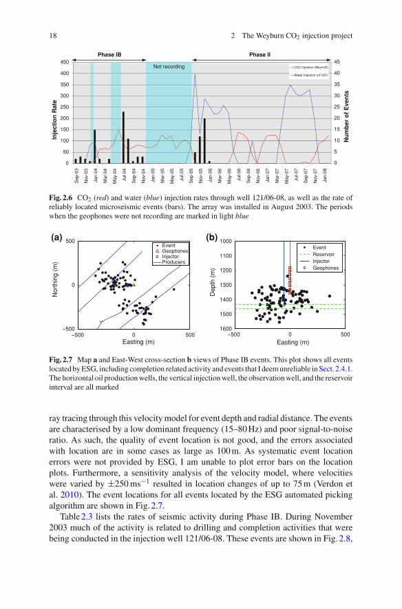
The rates of seismicity, the fluid injection rates in well 121/06-08 and periods whenthe geophones were not recording are plotted in Fig. 2.6, which shows monthly eventrates. Examples of daily event rates can be seen in Figs. 2.10 and 2.11. Events areclustered temporally, as most days have no events, but sometimes as many as 7 eventswill occur in the space of a few hours. Although some seismicity is recorded duringthe initial stages of Phase II, there are no events at all for over 2 years from 2006.

2.4.1 Phase IB

In order to compute locations, a 1-D velocity model was computed using a dipolesonic velocity log from a nearby well. Event locations were provided by ESG, havingbeen computed using P-wave particle motion for arrival azimuth and P- and S-wave


0

5

10

15

20

25

30

35

40

45

0

50

100

150

200

250

300

350

400

450

Sep

-03

Nov

-03

Jan-

04

Mar

-04

May

-04

Jul-0

4

Sep

-04

Nov

-04

Jan-

05

Mar

-05

May

-05

Jul-0

5

Sep

-05

Nov

-05

Jan-

06

Mar

-06

May

-06

Jul-0

6

Sep

-06

Nov

-06

Jan-

07

Mar

-07

May

-07

Jul-0

7

Sep

-07

Nov

-07

Jan-

08

Inje

ctio

n R

ate

CO2 Injection (Mscm/D)

Water Injection (m^3/D)

Not recording

Phase IB Phase II

Nu

mb

er o

f E

ven

ts

Fig. 2.6 CO2 (red) and water (blue) injection rates through well 121/06-08, as well as the rate ofreliably located microseismic events (bars). The array was installed in August 2003. The periodswhen the geophones were not recording are marked in light blue

−500 0 500−500

0

500

Easting (m)

Nor

thin

g (m

)

EventGeophonesInjectorProducers

−500 0 500

1000

1100

1200

1300

1400

1500

1600

Easting (m)

Dep

th (

m)

EventReservoirInjectorGeophones

(a) (b)

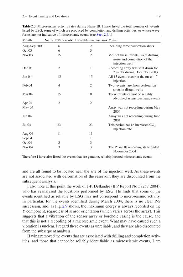
Fig. 2.7 Map a and East-West cross-section b views of Phase IB events. This plot shows all eventslocated by ESG, including completion related activity and events that I deem unreliable in Sect. 2.4.1.The horizontal oil production wells, the vertical injection well, the observation well, and the reservoirinterval are all marked

ray tracing through this velocity model for event depth and radial distance. The eventsare characterised by a low dominant frequency (15–80 Hz) and poor signal-to-noiseratio. As such, the quality of event location is not good, and the errors associatedwith location are in some cases as large as 100 m. As systematic event locationerrors were not provided by ESG, I am unable to plot error bars on the locationplots. Furthermore, a sensitivity analysis of the velocity model, where velocitieswere varied by ±250 ms−1 resulted in location changes of up to 75 m (Verdon etal. 2010). The event locations for all events located by the ESG automated pickingalgorithm are shown in Fig. 2.7.

Table 2.3 lists the rates of seismic activity during Phase IB. During November2003 much of the activity is related to drilling and completion activities that werebeing conducted in the injection well 121/06-08. These events are shown in Fig. 2.8,

2.4 Event Timing and Locations 19

Table 2.3 Microseismic activity rates during Phase IB. I have listed the total number of ‘events’listed by ESG, some of which are produced by completion and drilling activities, or whose wave-forms are not indicative of microseismic events (see Sect. 2.4.1)

Month No. of ESG ‘events’ Locatable microseisms Notes

Aug–Sep 2003 6 2 Including three calibration shotsOct 03 6 3Nov 03 15 2 Most of these ‘events’ were drilling

noise and completion of theinjection well

Dec 03 2 1 Recording array was shut down for2 weeks during December 2003

Jan 04 15 15 All 15 events occur at the onset ofinjection

Feb 04 4 2 Two ‘events’ are from perforationshots in distant wells

Mar 04 15 0 These events cannot be reliablyidentified as microseismic events

Apr 04 2 2May 04 Array was not recording during May

2004Jun 04 Array was not recording during June

2004Jul 04 23 23 This period has an increased CO2

injection rateAug 04 11 11Sep 04 1 1Oct 04 3 3Nov 04 3 3 The Phase IB recording stage ended

November 2004

Therefore I have also listed the events that are genuine, reliably located microseismic events

and are all found to be located near the site of the injection well. As these eventsare not associated with deformation of the reservoir, they are discounted from thesubsequent analysis.

I also note at this point the work of J-P. Deflandre (IFP Report No 58257 2004),who has reanalysed the locations performed by ESG. He finds that some of theevents identified as reliable by ESG may not correspond to microseismic activity.In particular, for the events identified during March 2004, there is no clear P-Ssuccession, and, as Fig. 2.9 shows, the maximum energy is always recorded on theY component, regardless of sensor orientation (which varies across the array). Thissuggests that a vibration of the sensor array or borehole casing is the cause, andthat this is not a recording of a microseismic event. What may have caused such avibration is unclear. I regard these events as unreliable, and they are also discountedfrom the subsequent analysis.

Having removed the events that are associated with drilling and completion activ-ities, and those that cannot be reliably identifiable as microseismic events, I am


−500 0 500−500

0

500

Easting (m)

Nor

thin

g (m

)

−500 0 500

1000

1100

1200

1300

1400

1500

1600

Easting (m)

Dep

th (

m)

(a) (b)

Fig. 2.8 Map a and EW cross-section b views of seismic emissions detected during drilling andcompletion activities in injection well 121/06-08. The events are all located near the injection well,marked on b in blue. Wells are marked as per Fig. 2.7

0.0 0.5 1.0 1.5 2.0

Time (s)

12

34

56

78

Geo

phon

e nu

mbe

r

Fig. 2.9 A typical ‘event’ from March 2004, recorded on all 8 geophones listed in Table 2.2, on X(red), Y (blue) and Z (green) components. Note that the maximum energy is always recorded on theY component, regardless of the sensor orientation, which varies across the array. Hence the wavescan not be reliably identified as coming from a microseismic event

left with 68 microseismic events for the period August 2003 to November 2004.This is a very low rate of seismicity in comparison to the 100s or even 1000s ofevents recorded per month at other producing carbonate reservoirs such as Ekofisk,Valhall (North Sea) and Yibal (Oman) (Dyer et al. 1999; Jones et al. 2010; Al-Harrasiet al. 2010). Figure 2.10 shows the locations for the remaining events that are reli-ably identified. The events can be divided into 2 clusters, one to the northwest of theinjection well towards production well 191/11-08, and one to the southeast of theinjection well, around production well 192/09-06.

The first cluster of events is located to the southeast of the injection well, aroundthe horizontal production well 192/09-06. These events are all located in and just


−500 −250 0 250 500−500

−250

0

250

500

Easting (m)

Nor

thin

g (m

)

−500 −250 0 250 500

1000

1100

1200

1300

1400

1500

1600

Easting (m)

Dep

th (

m)

(a) (b)

Fig. 2.10 Map a and EW cross-section b views of reliably located Phase IB microseismic events.Wells are marked as per Fig 2.7. The events are colour-coded by time of occurrence: yellow = pre-injection (Aug–Dec 2003), magenta = initial injection period (Jan–Apr 2004), red = during elevatedinjection rate period (Jul–Nov 2004). The events are found near the producing wells to the NWand SE

Fig. 2.11 Comparison of production rates from well 192/09-06 with the rate of microseismicity inthe nearby SE cluster. Microseismic activity occurs when production is temporarily stopped. Basedon Weyburn Microseismic Progress Report, ESG, Canada, April 2004

above the reservoir. These events occur throughout the monitoring period, includingthe period before injection. Comparison with production data for well 192/09-06(Fig. 2.11) indicates that the timing of the events correlates with periods where pro-duction is temporarily stopped. It is likely that these events are being generatedby pressure increases around the well that result from the temporary cessation ofpumping. Therefore these events are probably not directly related to CO2 injection.

The second cluster of events is located between the injection well and the hor-izontal production well 191/11-08 to the NW. The first of these events occur on


Fig. 2.12 Comparison of CO2 injection rate with microseismicity rate in the nearby NW cluster.Based on Verdon et al. (2010)

January 21st, coincident with the initiation of CO2 injection. Microseismicity occursat the onset of injection, and also appears to be correlated with periods of increasedinjection (Fig. 2.12), although unfortunately the recording system was locked outduring the period with maximum injection rate. The event locations mark a cloudof microseismicity which centres on the production well. Some events are locatedbetween the production and injection wells, while some events are located to theNW of the production well. The majority of events are located above the reservoir,although some events are located within the reservoir interval, and some are locatedbelow it.

A histogram of event depths during Phase IB is plotted in Fig. 2.13. Many eventsappear to be located above the reservoir. Although the large depth errors mean thatsome of these could actually be located within the reservoir interval, it is clear thatat least some activity must be occurring in the overburden. This is an interestingobservation, and without geomechanical modelling it is not clear whether this couldrepresent fluid migration or merely stress transfer into the overburden.

The event magnitudes are plotted in Fig. 2.14 as a function of distance. Eventmagnitudes range between −3 and −1. Event magnitudes of −2 are still detectableeven at a distance of over 400 m. Small events are still detectable at large distances,which suggests that the small number of events recorded is not an artifact of highnoise levels. Figure 2.14 suggests that surface arrays would have limited use formicroseismic monitoring under these conditions. The largest events recorded havemagnitudes less than −1.0, and many are smaller than −2.0. Dense surface arrayswould be required to detect such events, and their detectability would be stronglyinfluenced by surface noise and the nature of event focal mechanisms.


Fig. 2.13 Histogram ofevent depths for reliablylocated microseismic eventsdetected during Phase IB.The reservoir interval ismarked. Many events arelocated above the reservoir

0 1 2 3 4 5 6 7

1300

1350

1400

1450

1500

1550

Dep

th (m

)

Fig. 2.14 Event magnitudes at Weyburn plotted as a function of distance from the array. Based onVerdon et al. (2010). The line marks the limit of detectability as a function of distance from thearray

2.4.2 Phase II

Recording for Phase II runs from October 2005 to the present. Although there aredata recorded on the geophones, the majority of these represent near surface noiseor electrical spikes. Only 39 have been reliably identified as microseismic events,occurring in two temporal clusters, with 18 events at the end of October 2005 and21 in mid-January 2006. The Phase II events were located by ESG using the samemethod and velocity model as described for Phase IB above. The event locations ascomputed by ESG are plotted in Fig. 2.15.

The October 2005 events are located close to the observation well at a rangeof depths, from 900 to 1500 m, but usually above reservoir depth. The mechanismcausing these events is as yet unidentified. The majority of the January events cluster


−500 0 500−500

0

500

Easting (m)

Nor

thin

g (m

)

−500 0 500

1000

1100

1200

1300

1400

1500

1600

Easting (m)

Dep

th (m

)

(a) (b)

Fig. 2.15 Map view a and EW cross section b of microseismic events recorded during Phase II.Events are broken up into two clusters occurring in October 2005 (red) and January 2006 (blue).The majority of the January 2006 events are located within one cluster to the SE. Wells are markedas per Fig. 2.7

to the southeast of the observation well at reservoir depths. The field operator hasattributed these events to completion activities in a nearby borehole. As such, onlythe 18 October 2005 events are microseisms, and of these only a minority occurin or close to the reservoir. Over 3 years of recording this represents a remarkablylow rate of seismicity, continuing the trend already noted in Phase IB. Gaining anunderstanding of why activity is so low may well be more informative than thelocations of the few events that are available.

2.5 Discussion

The temporal clustering of microseismic events is episodic (Fig. 2.6) which raises thequestion of what causes these discrete episodes of localised deformation. If the eventswith a low dominant frequency are interpreted as fluid movement, why are they seenonly occasionally when fluid movement is occurring continuously? Focal mechanismanalysis can provide information here. For example fluid movement would perhapsgenerate non-double-couple mechanisms. Double-couple mechanisms describe rockfailure in a pure shear mode, where there is no volume change during failure. Wherevolume change occurs, perhaps induced by fluid filling a new fracture and proppingit open, then the focal mechanism would indicate not only shear failure but volumeincrease as well. Focal mechanism analysis could also image the triaxial stress tensorin the reservoir. This would provide important information for guiding injectionstrategies and groundtruthing geomechanical models. However, focal mechanismanalysis cannot be done with a single well array as at Weyburn.

Another important point is whether or not microseismicity above the reservoirindicates top-seal failure and the migration of CO2 into the overburden. Stress arch-ing effects, where loading of the reservoir transfers stress into the overburden, canalso lead to failure in the overburden and sideburden, without any fluid leaving the

2.5 Discussion 25

reservoir. To determine whether or not deformation results in increased fault perme-ability it is necessary to consider the rheology of the rock with respect to the stressesat the time of faulting. This underscores the importance of having a good understand-ing of the potential geomechanical behaviour of the storage site-it is likely that fluidmigration or a pore-pressure connection into the overburden will be documented by adifferent spatial and temporal pattern in seismicity from those associated with stressarching effects.

A key question is should CCS operations always/sometimes/never employ micro-seismic monitoring, and how should this decision be made? Downhole monitoring isnow a commonly used tool for monitoring hydraulic fracture stimulation. It presentsa low cost option for long term CCS monitoring. Ideally, such monitoring wouldrecord little seismicity, suggesting that the CO2 plume moves aseismically throughthe reservoir, inducing no significant rock failure, as seems to be the case at Weyburn.In total, over the entire Phase IB and Phase II microseismic monitoring experiment,only 86 reliably identifiable microseismic events were recorded in 5 years. How-ever, the lack of data has meant that the microseismic monitoring at Weyburn hasprovided little information about the reservoir stress state and injection inducedpressure fronts. Microseismic monitoring can be viewed as an early warning system,where large swarms of events in unexpected locations could be used to indicate thatthere is a risk of leakage. Paradoxically then, we should be placing geophones in theground in the hope that they detect nothing. Other monitoring techniques deployed atWeyburn, such as soil gas flux monitoring and shallow aquifer sampling, are similarin the way that detection of nothing represents a success.

Should the lack of microseismicity seen at Weyburn always be expected for CO2injection scenarios? It has been suggested that, as it has a lower compressibility,CO2 will have an inherently lower seismic deformation efficiency than other com-mon injection fluids such as water. Seismic deformation efficiency describes the ratiobetween the energy used in pumping a fluid into the formation and the total seismicenergy recorded on the geophones (e.g., Maxwell et al. 2008). If this is the case, thenmicroseismic monitoring is less likely to be useful for CCS activities. Alternatively,there may be geomechanical explanations for the lack of microseismic activity atWeyburn. In the following chapter I will discuss shear wave splitting measurementsmade on the Weyburn microseismic data, developing a novel approach to invertsplitting measurements for fracture properties. I will then switch my focus from themicroseismic data and instead seek to explain the lack of it. To do this I will con-sider another microseismic dataset from a different CO2 injection site, and constructrepresentative geomechanical models that approximate the Weyburn reservoir.

2.6 Summary

• CO2 storage and enhanced oil recovery has been ongoing at Weyburn since 2000.A downhole geophone array was installed in 2003 to monitor microseismicity inone pattern.


• The array has detected microseismicity, and events have been located by ESGusing automated location algorithms.

• I have manually sorted the events between those that can be reliably identified asmicroseismic events, those that are due to operator activities (perf-shots, drilling,etc.), and have discarded those that where a clear P- and S-wave succession cannotbe identified.

• 86 microseismic events have been located over 5 years of monitoring. This repre-sents a low rate of microseismicity relative to many producing carbonate fields.

• Events during Phase IB can be divided into in 2 clusters, near the production wellsto the NW and SE. Rates of seismicity can be correlated with activities in thesewells.

• Although depth errors are large, events do appear to be located in the overbur-den. Without geomechanical modelling it is not clear whether this represents fluidmigration from the reservoir, or merely failure induced by stress transfer into theoverburden.

• The low rates of microseismicity, combined with only one array, means that it hasnot been possible to image the triaxial stress state in the reservoir, nor to trackpressure or fluid migration fronts.

References

Al-Harrasi O, Al-Anboori A, Wüstefeld A, Kendall J-M (2010) Seismic anisotropy in a hydrocarbonfield estimated from microseismic data. Geophys Prospect 59(2):227–243

Balmforth NJ, Craster RV, Rust AC (2005) Instability in flow through elastic conduits and volcanictremor. J Fluid Mech 527:353–377

Brown LT (2002) Integration of rock physics and reservoir simulation for the interpretation of time-lapse seismic data at Weyburn field Saskatchewan. Master’s thesis Colorado School of Mines,Golden Colorado

Dyer BC, Cowles RHJJF, Barkved O, Folstad PG (1999) Microseismic survey of a North Seareservoir. World Oil 220:74–78

Jones GA, Raymer D, Chambers K, Kendall JM (2010) Improved microseismic event location byinclusion of a priori dip particle motion: a case study from Ekofisk. Geophys Prospect 58:727–737

Li G (2003) 4D seismic monitoring of CO2 flood in a thin fractured carbonate reservoir. LeadingEdge 22:690–695

Maxwell SC, Shemeta J, Campbell E, Quirk D (2008) Microseismic deformation rate monitoringSPE 116596. Presented at the SPE Annual Technical Conference

Pendrigh NM (2004) Core analysis and correlation to seismic attributes, Weyburn Midale Pool,Southeastern Saskatchewan. In: Summary of investigations, Vol. 1 Saskatchewan GeologicalSurvey Sask. Ind Resour, Misc. Rep 1:2004-4.1

Verdon JP, White DJ, Kendall J-M, Angus DA, Fisher Q, Urbancic T (2010) Passive seismicmonitoring of carbon dioxide storage at Weyburn. Leading Edge 29(2):200–206

White DJ (2008) Geophysical monitoring in the IEA GHG Weyburn-Midale CO2 monitoring andstorage project. SEG Expand Abstr 27:2846–2849

White D (2009) Monitoring CO2 storage during EOR at the Weyburn-Midale field. Leading Edge28: pp 838–842

Wilson M, Monea M, Whittaker S, White D, Law D, Chalaturnyk R (2004) IEA GHG WeyburnCO2 Monitoring & Storage Project Summary Report 2000–2004. PTRC

http://www.springer.com/978-3-642-25387-4

the weyburn co2 injection project

Documents