the work-averse cyber attacker model: theory and...
TRANSCRIPT

The Work-Averse Cyber Attacker Model:Theory and Evidence From Two Million Attack Signatures
Luca Allodia, Fabio Massaccic,∗, Julian Williamsb
aDepartment of Mathematics and Computer Science,Eindhoven University of Technology, Eindhoven, The Netherlands.bDurham University Business School, Mill Hill Lane, Durham, UK.
cDepartment of Information Engineering and Computer Science, University of Trento, Trento, Italy.
Abstract
A common conceit is that the typical cyber attacker is assumed to be all powerful andable to exploit all possible vulnerabilities with almost equal likelihood. In this paper wepresent, and empirically validate, a novel and more realistic attacker model. The intuitionof our model is that a mass attacker will optimally choose whether to act and weaponizea new vulnerability, or keep using existing toolkits if there are enough vulnerable users.The model predicts that mass attackers may i) exploit only one vulnerability per softwareversion, ii) include only vulnerabilities with low attack complexity, and iii) be slow atintroducing new vulnerabilities into their arsenal. We empirically test these predictions byconducting a natural experiment for data collected on attacks against more than one millionreal systems by Symantec’s WINE platform. Our analysis shows that mass attackers fixedcosts are indeed significant and that substantial efficiency gains can be made by individualsand organizations by accounting for this effect.
Keywords: Cyber Security, Dynamic Programming, Malware Production, Risk ManagementJEL Classification: C61, C9, D9, L5
Vulnerabilities in an information systems allow cyber attackers to exploit these affectedsystems for financial and/or political gain. Whilst a great deal of prior research has focusedon the security investment decision making process for security vendors and targets, thechoices of attackers are less well understood. This paper is the first attempt to directlyparameterize cyber attacker production functions from first principles and the empiricallyfit this function to empirical data.
Our main results challenge the notion of all powerful attackers able to exploit a broadrange of security vulnerabilities and provides important guidance to policy makers and po-tential targets on how to utilize finite resources in the presence of cyber threats.1
∗Corresponding Author. The authors thank Matthew Elder at Symantec Corp. for his many usefulcomments. A preliminary treatments of this dataset and conceptual idea have been presented at the 2015European Conference on Information Systems (ECIS 2015). The authors retain copyright for future publi-cation purposes. This research has been partly supported from the European Union’s Seventh FrameworkProgramme for research, technological development and demonstration under grant agreement no 285223(SECONOMICS), from the Italian PRIN Project TENACE, and from the EIT Digital Master School 2016 -Security and Privacy programme. Our results can be fully reproduced by recovering the reference data setWINE-2012-008, archived in the WINE infrastructure.
Email addresses: [email protected] (Luca Allodi), [email protected] (Fabio Massacci),[email protected] (Julian Williams)
1An early security reference on this conceit can be found in (Dolev and Yao 1983a, page 199) where aprotocol should be secured “against arbitrary behavior of the saboteur”. The Dolev-Yao model is a quasi“micro-economic” security model: given a population with several (interacting) agents, a powerful attackerwill exploit any weaknesses, and security is violated if she can compromise some honest agent. So, everyagent must be secured by mitigating all vulnerabilities. A more gentle phrasing suggests that the likelihoodthat a given vulnerability is exploited should be at maximum entropy and hence the only dominating factorwill be the criticality of that vulnerability.
Preprint May 29, 2017

A natural starting point when attempting to evaluate the decision making of attackers isto look at the actual ‘traces’ their attacks leave on real systems (also referred as ‘attacks inthe wild ’): each attempt to attack a system using a vulnerability and an exploit mechanismgenerates a specific attack signature, which may be recorded by software security vendors.Dumitras and Shou (2011) and Bilge and Dumitras (2012) provide a summary of signatureidentification and recording, whilst Allodi and Massacci (2014) shows how they can be linkedto exploit technology menus. By observing the frequency with which these attack signaturesare triggered, it is possible to estimate (within some level of approximation) the rate ofarrival of new attacks. Evidence from past empirical studies suggests a different behaviordepending on fraud type; for example, Murdoch et al. (2010) shows that attackers focussingon chip and pin credit cards, which require physical access, are very proactive and rapidlyupdate their menu of exploits; for web users, Allodi and Massacci (2014) and Nayak et al.(2014) indicate that the actual risk of attacks in the wild is limited to hundred vulnerabilitiesout of the fifty thousand reported in vulnerability databases. Mitra and Ransbotham (2015)confirm these findings by showing that even (un)timely disclosures do not correlate withattack volumes.
These empirical findings are at odds with the classical theoretical models of attackerbehaviour by which attackers can and will exploit any vulnerability Dolev and Yao (1983a),and remain largely un-explained from a theoretical perspective. This paper fills this gap byidentifying a new attacker model that realistically unifies the attacker’s production functionwith empirical evidence of rates of arrival of new attacks worldwide. The current corpus ofresults provide strong prima-facie evidence that attackers do not quickly mass develop newvulnerability exploits that supplement or replace previous attack implementations. This col-lective behavior is at odds with the classical theoretical models of attacker behaviour Dolevand Yao (1983b): attackers should exploit any vulnerability. We must therefore concludethat attackers are rational, that the effort required to produce an exploit and hence deploy-able malware is costly, and that they will respond to incentives in a way that is consistentwith classical models of behaviour (Laffont and Martimort 2009). Finally, this work di-rectly impacts the development of risk models for cyber-attacks by identifying empirical andtheoretical aspects of attack and malware production.2
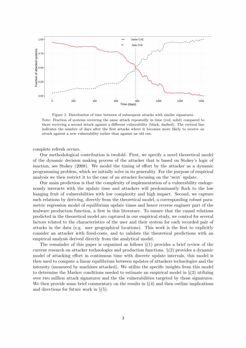
Figure 1 shows the fractions of systems receiving attacks recorded by Symantec, a largesecurity vendor, for two different cases: the red line plots the fraction of systems receivingtwo attacks at two different times that target the same software vulnerability (CVE). Theabscissa values represent the time, in days, between attacks, hence we would expect thatthe red line would decrease (which it does) from near unity to zero. The black dashed linerepresents the opposite case: the same system and the same software are attacked but theattacker uses a new vulnerability, different from the original attack. The attack data suggeststhat it takes more than two years before the number of attacks using new vulnerabilitiesexceeds the number of attacks using the same vulnerabilities, and about 3-4 years before a
2Whilst challenging the maximum entropy notion may initially appear to the informed reader as attackinga straw man, the underpinning ideas of Dolev-Yao persist into to the internet era (through all phases), seefor instance comments in Schneier (2008) that cover similar ground. Variants of the all-powerful attackers areproposed (e.g. honest-but-curious, game-based provable security models) but they only changed the powerand speed of attacks not the will: if there is weakness that the attacker can find and exploit, they will. Papersanalyzing web vulnerabilities Stock et al. (2013), Nikiforakis et al. (2014) report statistics on the persistenceof these vulnerabilities on internet sites as evidence for this all powerful effect and broad coverage of securityvulnerabilities. We would like to emphasize that we are not arguing, necessarily, that there is systematicover-investment in information security, but that presuming the probability mass function relating likelihoodof a successful attack to exploitable vulnerabilities, by severity category, is at or close to maximum entropyis sub-optimal for security investment decision making.
2
Same CVE
New CVE
0.00
0.25
0.50
0.75
1.00
0 200 400 600 800 1000 1200 1400Time (days)
Fra
ctio
n of
atta
cked
sys
tem
s
Figure 1: Distribution of time between of subsequent attacks with similar signatures.
Note: Fraction of systems receiving the same attack repeatedly in time (red, solid) compared tothose receiving a second attack against a different vulnerability (black, dashed). The vertical lineindicates the number of days after the first attacks where it becomes more likely to receive anattack against a new vulnerability rather than against an old one.
complete refresh occurs.Our methodological contribution is twofold. First, we specify a novel theoretical model
of the dynamic decision making process of the attacker that is based on Stokey’s logic ofinaction, see Stokey (2008). We model the timing of effort by the attacker as a dynamicprogramming problem, which we initially solve in its generality. For the purpose of empiricalanalysis we then restrict it to the case of an attacker focusing on the ‘next’ update.
Our main prediction is that the complexity of implementation of a vulnerability endoge-nously interacts with the update time and attackers will predominantly flock to the lowhanging fruit of vulnerabilities with low complexity and high impact. Second, we capturesuch relations by deriving, directly from the theoretical model, a corresponding robust para-metric regression model of equilibrium update times and hence reverse engineer part of themalware production function, a first in this literature. To ensure that the causal relationspredicted in the theoretical model are captured in our empirical study, we control for severalfactors related to the characteristics of the user and their system for each recorded pair ofattacks in the data (e.g. user geographical locations). This work is the first to explicitlyconsider an attacker with fixed-costs, and to validate the theoretical predictions with anempirical analysis derived directly from the analytical model.
The remainder of this paper is organized as follows §(1) provides a brief review of thecurrent research on attacker technologies and production functions. §(2) provides a dynamicmodel of attacking effort in continuous time with discrete update intervals, this model isthen used to compute a linear equilibrium between updates of attackers technologies and theintensity (measured by machines attacked). We utilize the specific insights from this modelto determine the Markov conditions needed to estimate an empirical model in §(3) utilizingover two million attack signatures and the the vulnerabilities targeted by those signatures.We then provide some brief commentary on the results in §(4) and then outline implicationsand directions for future work in §(5).
3

1. Background
The economic decision making and the organization of information system security hasbeen explored from a target perspective quite thoroughly in recent years. Anderson (2008)provides a good summary on the early extant literature.3 Commonly, the presence of vul-nerabilities has been considered as the starting point for the analysis, as it could allow anattacker to take (total or partial) control of a system and subvert its normal operation forpersonal gain.
Asghari et al. (2013), Van Eeten and Bauer (2008), Van Eeten et al. (2010) address theeconomic incentives (either perverse or well aligned) in addressing security threats. Marketbased responses, such as bug bounty programs, are discussed in Miller (2007) and Frei et al.(2010) whilst Karthik Kannan (2005) and Finifter et al. (2013) also address the issue ofvulnerability markets and the value of vulnerabilities to developers, organizations that maypotentially be targeted, and indeed attackers.
The consensus in the security literature appears to have settled on the view that theseverity of the vulnerability, as measured by a series of metrics, should be used as a directanalogue of risk. For a broad summary of the metrics and risk assessments involved in thisdomain see Mellado et al. (2010) (technology based metrics); Sheyner et al. (2002), Wanget al. (2008), Manadhata and Wing (2011) (attack graphs and surfaces); and Naaliel et al.(2014), Wang et al. (2009), Bozorgi et al. (2010), Quinn et al. (2010) (severity measure metricsand indexation). From an economic perspective Ransbotham and Mitra (2009) studies theincentives that influence the diffusion of vulnerabilities and hence the opportunities of theattacker to attack a target’s systems (software and infrastructure). The standard de factometric for the assessment of vulnerability severity is the Common Vulnerability ScoringSystem, or CVSS4 in short CVSS-SIG (2015). Hence, the view is that any open vulnerabilitywill eventually be exploited by some form of malware and the target organization will thenbe subject to a cyber attack.
Recent studies in the academic literature have challenged the automatic transfer of thetechnical assessment of the ‘exploitability’ of a vulnerability into actual attacks against endusers. Bozorgi et al. (2010) and Allodi and Massacci (2014) have empirically demonstratedon different samples a substantial lack of correlation between the observed attack signaturesin the wild and the CVSS type severity metrics. The current trend in industry is to usethese values as proxies demanding immediate action (see Beattie et al. (2002) for operatingsystem security, PCI-DSS (2010) for credit card systems and Quinn et al. (2010) for USFederal rules).
In particular, prior work suggests that only a small subset of vulnerabilities are actuallyexploited in the wild (Allodi and Massacci 2014), and that none of the CVSS measures ofseverity of impact predict the viability of the vulnerability as a candidate for an implementedexploit (Bozorgi et al. 2010). Bozorgi et al. (2010) argue that besides the ‘technical’ measureof the system’s vulnerabilities, other factors should be considered such as the value or costof a vulnerability exploit and the ease and cost with which the exploit can be developed andthen deployed.
Mitra and Ransbotham (2015) also indicate that early disclosure has no impact on attackvolume (number of recorded attacks) and there is only some correlation between early dis-
3Policy, cost sharing and incentives have also been comprehensively explored from a target perspective inAugust and Tunca (2006, 2008, 2011) and Arora et al. (2004, 2008).
4The CVSS score provides a standardized framework to evaluate vulnerability severity over several metrics,and is widely reported in public vulnerability databases such as the National Vulnerability Database NIST(2015) maintained by the National Institute of Standards in Technology (NIST).
4
closure and the ‘time-to-arrival’ of exploits: hence providing additional evidence reinforcingthe lack of ‘en mass’ migration of attacks to newly disclosed vulnerabilities.
On a similar line, Herley (2013) posits the idea that for a (rational) attacker not all attacktypes make sensible avenues for investment. This is supported by empirical evidence showingthat attack tools actively used by attackers embed only ten to twelve exploits each on themaximum (Kotov and Massacci 2013, Grier et al. 2012), and that the vast majority of attacksrecorded in the wild are driven by only a small fraction of known vulnerabilities (Nayak et al.2014, Allodi 2015). It is clear that for the attacker some reward must be forthcoming, as thelevel of costly effort required to implement and deliver the attack observed in the wild is farfrom negligible. For example, Grier et al. (2012) uncovers the presence of an undergroundmarket where vulnerability exploits are rented to attackers (‘exploitation-as-a-service’) asa form of revenue for exploit writers. Liu et al. (2005) suggest that attacker economicincentives should be considered when thinking about defensive strategies: increasing attackcosts or decreasing revenue may be effective in deterring the development and deployment ofan attack. For example, Chen et al. (2011) suggests that a possible mean to achieve this is to‘diversify’ system configurations within an infrastructure so that the fraction of attackablesystem by a single exploit diminishes, hence lowering the return for any given attack.
The effort needed to engineer an attack can be generally characterized along the threeclassic phases from Jonsson and Olovsson (1997): reconnaissance (where the attacker iden-tifies potential victims), deployment (the engineering phase), refinement (when the attack isupdated). The first phase is covered by the works of Wang et al. (2008), Howard et al. (2005),Nayak et al. (2014), where the attacker investigates the potential pool of targets affected bya specific vulnerability by evaluating the attack surface of a system, or the ‘popularity’ ofa certain vulnerable software. The engineering aspects of an exploit can be understood byinvestigating the technical effort required to design one (see for example Schwartz et al.(2011) and Carlini and Wagner (2014) for an overview of recent exploitation techniques).However,the degree of re-invention needed to update an exploit and the anticipated timefrom phase two to phase three remain largely un-investigated (Yeo et al. 2014, Serra et al.2015, Bilge and Dumitras 2012, provide some useful results in this direction).
Our model aggregates deployment and reconnaissance costs into a single measure, whereaswe explicitly model the expected time to exploit innovation and subsequent updating timesto include new vulnerabilities.
2. A Dynamic Attacker Model with Costly Effort
We consider a continuous time setting, such that 0 < t < ∞, where an attacker willbe choosing an optimal update sequence 0 < T1 < T2 < . . . Ti . . . T∞ for weaponizing newvulnerabilities v1, .., vn. The attackers technology has a “combination” of exploit technologythat undergoes periodic updates. Each combination targets a specific mix of vulnerabilitiesand we presume that the attacker can make costly investments to develop the capability oftheir technology.
The attacker starts their development and deployment activity at time t = 0 by initiallyidentifying a set of vulnerabilities V ⊂ V from a large universe V affecting a large number oftarget systems N . A fraction θV of the N systems is affected by V and would be compromisedby an exploit in absence of security countermeasures. Targets are assumed to deploy patchesand/or update systems, whilst security products update their signatures (e.g. antiviruses,firewalls, intrusion prevention systems). Hence, the number of infected systems available forexploit will decay with time.
We can represent vulnerability patches and security signatures as arriving on users’ sys-tems following two independent exponential decay processes governed respectively by the
5
rates λp and λsig. The effect of λp and λsig on attacks has been previously discussed byArora et al. (2004, 2008), Chen et al. (2011), whilst a discussion on their relative magnitudeis provided in Nappa et al. (2015). Assuming that the arrival of patches and antivirus sig-natures are independent processes, and rolling them up into a single factor λ = f(λp, λsig),the number of systems impacted by vulnerabilities in V at time t is
NV (t) = NθV e−λt. (1)
For the given set of vulnerabilities V targeted by their technologies combination the attackerwill pay an upfront cost C(V |∅) and has an instantaneous stochastic profit function of
ΠV (t) = [r(t,NV (t), V )− c(t, V )]e−δt, (2)
where r(t,NV , V ) is a stochastic revenue component5, whilst c(t, V ) is the variable costs ofmaintaining the attack6, subject to a discount rate of δ. We do not make any assumptionon the form that revenues take from successful attacks. They could be kudos in specific fora(Ooi et al. 2012) or revenues from trading the victim’s assets in underground markets (Grieret al. 2012, Allodi et al. 2015).
At some point, the attacker might decide to perform a refresh of its attacking capa-bilities by introducing a new vulnerability and engineering its exploit by incurring an up-front cost of C(v|V ). This additional vulnerability will produce a possibly larger revenuer(t,NV ∪{v}(t), V ∪ {v}) at an increased marginal cost c(t, V ∪ {v}). As the cost of engineer-ing an exploit is large with respect to maintenance (C(v|V ) � c(t, V ∪ {v})) and neithersuccessful infection (Allodi et al. 2013), nor revenues are guaranteed (Herley and Florencio2010, Rao and Reiley 2012, Allodi et al. 2015), the attacker is essentially facing a problemof deciding action vs inaction in presence of fixed initial costs as described by Stokey (2008)and their best strategy is to deploy the new exploit only when the old vulnerabilities nolonger guarantee a suitable expected profit.
This decision problem is then repeated over time for n newly discovered vulnerabilities,and n refresh times denoted by Ti.
We define by C0 = C(V |∅) the initial development cost and by Ci+1 ≡ C(vi+1|V ∪{v1 . . . vi}) the cost of developing the new exploits, given the initial set V and the additionalvulnerabilities v1 . . . vi. We denote by Ni(t) ≡ NV ∪{v1,...,vi}(t) the number of systems affectedby adding the new vulnerability at time t. Similarly, we define ri(t) and ci(t) as the respectiverevenue and marginal cost of the vulnerability set V ∪ {v1, . . . , vi}. Then the attacker facesthe following stochastic programming problem for n→∞
{T ∗1 , . . . , T ∗n} = arg max{T1,...,Tn}
n∑i=0
−Cie−δTi +
∫ Ti+1
Ti
(ri(t,Ni(t))− ci(t)) e−δtdω. (3)
The action times T0 = 0, Ti+1 > Ti, and Tn+1 is such that rn(Tn+1, Nn(Tn+1)) = cn(Tn+1).Since the maintenance of malware, for example through ‘packing’ and obfuscation (i.e. tech-niques that change the aspect of malware in memory to avoid detection), is minimal and does
5This component accounts for the probability of establishing contact with vulnerable system (Franklinet al. 2007), the probability of a successful infection given a contact (Kotov and Massacci 2013, Allodi et al.2013), and the monetization of the infected system (Kanich et al. 2008, Zhuge et al. 2009, Rao and Reiley2012).
6For example, the attacker may need to obfuscate the attack payload to avoid detection (Grier et al. 2012),or renew the set of domain names that the malware contacts to prevent domain blacklisting (Stone-Grosset al. 2009).
6
not depend on the particular vulnerability, see (Brand et al. 2010, § 3) for a review of thevarious techniques, we have that ci(t)→ 0 and therefore also Tn+1 →∞. This problem canbe tractably solved with the techniques discussed in Stokey (2008), Birge (2010) and furtherdeveloped in Birge and Louveaux (2011) either analytically or numerically by simulation.Nevertheless, it is useful to impose some further mild assumptions that result in solutionswith a clean set of predictions that motivate and place in context our empirical work in thestandard Markovian set-up needed to identify specific effects.
By imposing the history-less (adapted process) assumption on the instantaneous payoff,with a risk neutral preference, the expected pay-off and expected utility for a given set ofordered action times {T1, . . . , Tn} coincides. Risk preferences are therefore encapsulatedpurely in the discount factor, a common assumption in the dynamic programming literature(see the opening discussion on model choice in (Stokey 2008, Ch. 1) for a review).
Following (Birge and Louveaux 2011, Ch. 4) the simplest approach is to presume risk neu-trality (under the discount factor δ) and solve in expectations as a non-stochastic Hamilton–Jacobi–Bellman type problem along the standard principles of optimal decision making.
Under the assumption of stationary revenues, we define r as the average revenue across allsystems. The instantaneous expected time t payoff from deployed malware is approximatedby the following function:
E[r(t,NV ∪{v}(t))].= rN
(θV e
−λt + (θV ∪{v} − θV )e−λ(t−T )), (4)
where t ≥ T is the amount of time since the attacker updated the menu of vulnerabilities (byengineering new exploits) at time T . The first addendum caters for the systems vulnerableto the set V of exploited vulnerabilities that have been already partly patched, whilst thesecond addendum accounts for the new, different systems that can be exploited by adding vto the pool. For the latter systems, the unpatched fraction restarts from one at time T .
Solving Eq. (3) in expectations we can replace the stochastic integral over dω with atraditional Riemann integral over dt and evaluate the approximation in expectations. Bysolving the above integral and imposing the usual first order condition we obtain the followingdecomposition for the optimal profit for the attacker.
{T ∗1 , . . . , T ∗n} = arg max{T1,...,Tn}
n∑i=0
(Π(Ti+1, Ti)− Ci)e−δTi (5)
Π(Ti+i, Ti) =rN
λ+ δ
(θi − θi−1 + θi−1e
−λTi)(
1− e−(λ+δ)(Ti+1−Ti))
(6)
where we abbreviate θ−1 ≡ 0, θ0 ≡ θV , and θi ≡ θV ∪{v1...vi}.
Proposition 1. The optimal times to weaponize and deploy new exploits for attackers awareof initial fixed costs of exploit development are obtained by solving the following n equationsfor i = 1, . . . , n
∂Π(Ti, Ti−1)
∂Tie−δTi−1 − δ(Π(Ti+1, Ti)− Ci)e−δTi +
∂Π(Ti+1, Ti)
∂Tie−δTi = 0 (7)
subject to T0 = 0, Tn+1 =∞, δ, λ > 0.
Proof of Proposition 1 is given in Appendix 6.1. �Unrestricted dynamic programming problems such as that described in Proposition 1
typically do not generally have analytic solutions for all parameter configurations. They canbe log-solved either in numerical format, or by computer algebra as a system of n equations by
7

setting xi = e−λTi , yi = e−δTi and then adding the n equations δ log xi = λ log yi. However,we can relax the solution procedure to admit a myopic attacker who only considers a singleindividual decision n = 1. This approximates the case when the true dynamic programmingproblem results in T ∗1 > 0 and T ∗2 →∞. For an overview of the appropriate domains for theuse of this type of simplification see DeGroot (2005).
Corollary 1. A myopic attacker, who anticipates an adapted revenue process from de-ployed exploits subject to a decreased effectiveness due to patching and anti-virus updateswith a negligible cost of maintenance for each exploit, will postpone indefinitely the choiceof weaponizing a vulnerability v if the ratio between the cost of developing the exploit andthe maximal marginal expected revenue is larger than the discounted increase in the frac-tion of exploited vulnerabilities, namely C(v|V )
rN > δλ+δ (θV ∪{v} − θV ). The attacker would
be indifferent to the time at which deploy the exploit only when the above relation holds atequality.
Proof of Corollary 1 is given in Appendix 6.2. �
Whilst our focus is on realistic production functions for the update of malware, it shouldbe noted that the ‘all–powerful’ attacker is still admitted under our solution if the attackercost function C(v|V ) for weaponizing a new vulnerability collapses to zero. In this case,Corollary 1 predicts that the attacker could essentially deploy the new exploit at an arbitrarytime [0,+∞] even if the new exploit would not yield extract impact (θV ∪{v} = θv).
If the vulnerability v affects a software version for which there is already a vulnerabilityin V ,the fraction of systems available for exploit will be unchanged (θv = θ). Hence, thecost has to be essentially close to zero (C(v|V ) → 0) for the refresh to be worth. In theempirical analysis section §(4) we report a particular case where we observe this phenomenonoccurring in our dataset. Based on these considerations we can now state our first empiricalprediction.
Hypothesis 1. Given Corollary 1, a work-averse attacker will overwhelmingly use only onereliable exploit per software version.
Engineering a reliable vulnerability exploit requires the attacker to gather and processtechnical vulnerability information (Erickson 2008).
This technical ‘exploit complexity’ is captured by the Attack Complexity metric pro-vided in the CVSS. When two vulnerabilities cover essentially the same population (θV ∪{v}−θV ≈ ε) a lower cost would make it more appealing for an attacker to refresh their arsenal
as this would make it easier to reach the condition (C(v|V )rN ≈ δ
λ+δ (θV ∪{v} − θV ) ≈ ε) whenthe attacker would consider deploying an exploit to have a positive marginal benefit.
Hypothesis 2. Corollary 1 also implies that a work-averse attacker will preferably deploylow-complexity exploits for software with the same type of popularity.
Corollary 1 describes a result in the limit and in presence of a continuous profit function.Indeed according to Eq. (4) the attacker expects to make a marginal profit per unit of
time equal to rNf(t) where limt→∞ f(t) → 0 and as a result ∂Π(Ti+1,Ti)∂Ti+1
is a monotone
decreasing function and ∂Π(Ti+1,Ti)∂Ti+1
→ 0 for Ti+1b→∞. In practice, the profit expectationsof the attacker are discrete: as the marginal profit drops below r, it is below the expectmarginal profit per unit of compromised computers. Hence, the attacker will consider thetime Ti+1 = T ? <∞ where such event happens as equivalent to the event where the marginalprofit goes to zero (Ti+1 = ∞) and hence assumes that the maximal revenue has beenachieved and a new exploit can be deployed.
8

Proposition 2. A myopic attacker, who anticipates an adapted revenue process from de-ployed exploits subject to a decreased effectiveness due to patching and anti-virus updates witha negligible cost of maintenance for each exploit, and expects a marginal profit at least equalto the marginal revenue for a single machine (∂Π
∂T ≥r(0,NV (0),V )
NV (0) ) will renew their exploit at
T ? =1
δlog
(C(v|V )
r− δ
λ+ δ(θV ∪{v} − θV )N
)(8)
under the condition that C(v|V )rN ≥ 1
N + δλ+δ (θV ∪{v} − θV ).
Proof of Proposition 2 is given in Appendix 6.3. �Assuming the cost and integral of the reward function over [0, T ∗i ] are measured in the
same numeraire and approximately within the same order of magnitude, the model impliesthat the discount factor plays a leading role in determining the optimal time for the newexploit deployment, the term 1
δ in Eq. (8). Typically the extant microeconomics literature(see Frederick et al. 2002) sets exp(δ)− 1 to vary between one and twenty percent. Hence, alower bound on T ∗1 would be ≈ [100, 400] when time is measured in days. This implies thefollowing prediction:
Hypothesis 3. Given Proposition 2, the time interval after which a new exploit wouldeconomically dominate an existing exploit is large, T ∗1 > 100 days.
3. Experimental Data Set
Our empirical dataset merges three data sources, these are:The National Vulnerability Database (NVD) is the vulnerability database main-
tained by the US. Known and publicly disclosed vulnerabilities are published in this datasetalong with descriptive information such as publication date, affected software, and a tech-nical assessment of the vulnerability as provided by the CVSS. Vulnerabilities reported inNVD are identified by a Common Vulnerabilities and Exposures identifier (CVE-ID) that isunique for every vulnerability.
The Symantec threat report database (SYM) reports the list of attack signaturesdetected by Symantec’s products along with a description in plain English of the attack.Amongst other information, the description reports the CVE-ID exploited in the attack, ifany.
The Worldwide Intelligence Network Environment (WINE), maintained by Syman-tec, reports attacks detected in the wild by Symantec’s products. In particular, WINE isa representative, anonymized sample of the operational data Symantec collects from usersthat have opted in to share telemetry data (Dumitras and Shou 2011). WINE comprisesattack data from more than one million hosts, and for each of them, we are tracking up tothree years of attacks. Attacks in WINE are identified by an ID that identifies the attacksignature triggered by the detected event. To obtain the exploited vulnerability we matchthe attack signature ID in WINE with the CVE-ID reported in SYM.
The data extraction involved three phases: (1) reconstruction of WINE users’ attackhistory; (2) building the controls for the data; (3) merging and aggregating data from (1)and (2). Because of user privacy concerns and ethical reasons, we did not extract from theWINE dataset any potentially identifying information about its hosts. For this reason, it isuseful to distinguish two types of tables: tables computed from WINE, namely intermediatetables with detailed information that we use to build the final dataset; and extracted tables,
9

Table 1: Variables included in our dataset
Variable Description
CVE1,2 The identifier of the previous and the current vulnerability v exploited on the user’smachine.
T The delay expressed in fraction of year between the first and the second attack.N The number of detected attacks for the pair previous attack, actual attack.U The number of systems attacked by the pair.Compl The Complexity of the vulnerability as indicated by its CVSS assessment. Can be
either High, Medium or Low as defined by CVSS(v2) Mell et al. (2007).Imp The Impact of the vulnerability measured over the loss in Confidentiality, Integrity
and Availability of the affected information. It is computed on a scale from 0 to 10where 10 represents maximum loss in all metrics, and 0 represents no loss. Mell et al.(2007).
Day The date of the vulnerability publication on the National Vulnerability Database.Sw The name of the software affected by the vulnerability.Ver The last version of the affected software where the vulnerability is present.Geo The country where the user system is at the time of the second attack.Hst The profile of the user or “host”. See Table 2 for reference.Frq The average number of attacks received by a user per day. See Table 2.Pk The maximum number of attacks received by a user per day. See Table 2.
containing only aggregate information on user attacks that we use in this research. The fulllist of variables included in our dataset and their description is provided in Table 1.7
3.1. Understanding the Attack Data Records
Each row in our final dataset of tables extracted from WINE represents an “attack-pair”received by Symantec users. We are interested in the new vulnerability v whose exploit hasbeen attempted after an exploit for V vulnerabilities have been already engineered. Hence,for every vulnerability v identified by CVE2 our dataset reports the aggregated number ofattacked users (U) and the aggregated volume of attacks (N ) on the vulnerability v whichhave previously (T days before) received an attack on some other vulnerability identified byCVE1.
Additional information regarding both attacked CVEs is extracted from the NVD: foreach CVE we collect the publication date (Day), the vulnerable software (Sw), the last vul-nerable version (Ver), and an assessment of the Compl of the vulnerability exploitation andof its Imp, as provided by CVSS (v2). At the time of performing the experiment we use thesecond revision of the CVSS standard.
A CVE may have more than one attack signature. This is not a problem in our dataas we are concerned with the exploitation event, and not with the specific footprint of theattack. However, attack signatures have varying degrees of generality, meaning that theycan be triggered by attacks against different vulnerabilities but follow some common pattern.For this reason, some signatures reference more than one vulnerability.
7Researchers interested in replicating our experiments can find NVD publicly available at http://nvd.
nist.gov; SYM is available online by visiting http://www.symantec.com/security_response/landing/
threats.jsp. The version of SYM and NVD used for the analysis is also available from the authors atanonymized_for_the_submission; the full dataset computed from WINE was collected in July 2013 and isavailable for sharing at Symantec Research Labs (under NDA clauses for access to the WINE repository)under the reference WINE-YYYY-NNN. In the online Appendix 7 we provide a full ‘replication guide’ thatinterested researchers may follow to reproduce our results from similar sources by Symantec or other securityvendors.
10
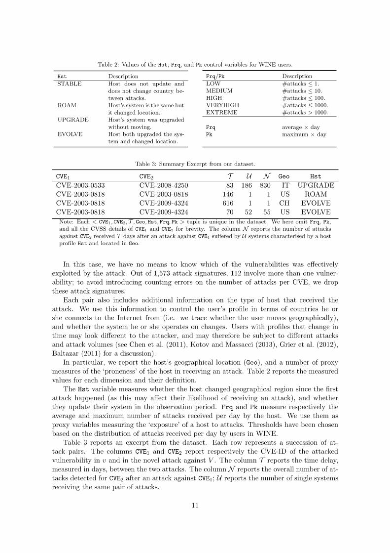
Table 2: Values of the Hst, Frq, and Pk control variables for WINE users.
Hst Description
STABLE Host does not update anddoes not change country be-tween attacks.
ROAM Host’s system is the same butit changed location.
UPGRADE Host’s system was upgradedwithout moving.
EVOLVE Host both upgraded the sys-tem and changed location.
Frq/Pk Description
LOW #attacks ≤ 1.MEDIUM #attacks ≤ 10.HIGH #attacks ≤ 100.VERYHIGH #attacks ≤ 1000.EXTREME #attacks > 1000.
Frq average × dayPk maximum × day
Table 3: Summary Excerpt from our dataset.
CVE1 CVE2 T U N Geo Hst
CVE-2003-0533 CVE-2008-4250 83 186 830 IT UPGRADECVE-2003-0818 CVE-2003-0818 146 1 1 US ROAMCVE-2003-0818 CVE-2009-4324 616 1 1 CH EVOLVECVE-2003-0818 CVE-2009-4324 70 52 55 US EVOLVE
Note: Each < CVE1, CVE2, T , Geo, Hst, Frq, Pk > tuple is unique in the dataset. We here omit Frq, Pk,and all the CVSS details of CVE1 and CVE2 for brevity. The column N reports the number of attacksagainst CVE2 received T days after an attack against CVE1 suffered by U systems characterised by a hostprofile Hst and located in Geo.
In this case, we have no means to know which of the vulnerabilities was effectivelyexploited by the attack. Out of 1,573 attack signatures, 112 involve more than one vulner-ability; to avoid introducing counting errors on the number of attacks per CVE, we dropthese attack signatures.
Each pair also includes additional information on the type of host that received theattack. We use this information to control the user’s profile in terms of countries he orshe connects to the Internet from (i.e. we trace whether the user moves geographically),and whether the system he or she operates on changes. Users with profiles that change intime may look different to the attacker, and may therefore be subject to different attacksand attack volumes (see Chen et al. (2011), Kotov and Massacci (2013), Grier et al. (2012),Baltazar (2011) for a discussion).
In particular, we report the host’s geographical location (Geo), and a number of proxymeasures of the ‘proneness’ of the host in receiving an attack. Table 2 reports the measuredvalues for each dimension and their definition.
The Hst variable measures whether the host changed geographical region since the firstattack happened (as this may affect their likelihood of receiving an attack), and whetherthey update their system in the observation period. Frq and Pk measure respectively theaverage and maximum number of attacks received per day by the host. We use them asproxy variables measuring the ‘exposure’ of a host to attacks. Thresholds have been chosenbased on the distribution of attacks received per day by users in WINE.
Table 3 reports an excerpt from the dataset. Each row represents a succession of at-tack pairs. The columns CVE1 and CVE2 report respectively the CVE-ID of the attackedvulnerability in v and in the novel attack against V . The column T reports the time delay,measured in days, between the two attacks. The column N reports the overall number of at-tacks detected for CVE2 after an attack against CVE1; U reports the number of single systemsreceiving the same pair of attacks.
11
*
**
** ** ****
************************
****
******
*****
******
**
0.0 0.5 1.0 1.5 2.0 2.5 3.0 3.5
01
23
45
67
Distrib. of the attacks received each day by user
Log scale of number of attacks per user (e.g. 3 = 1000attacks)
Log−
scal
e nu
mbe
r of u
sers
that
rece
ives
that
man
y at
tack
s
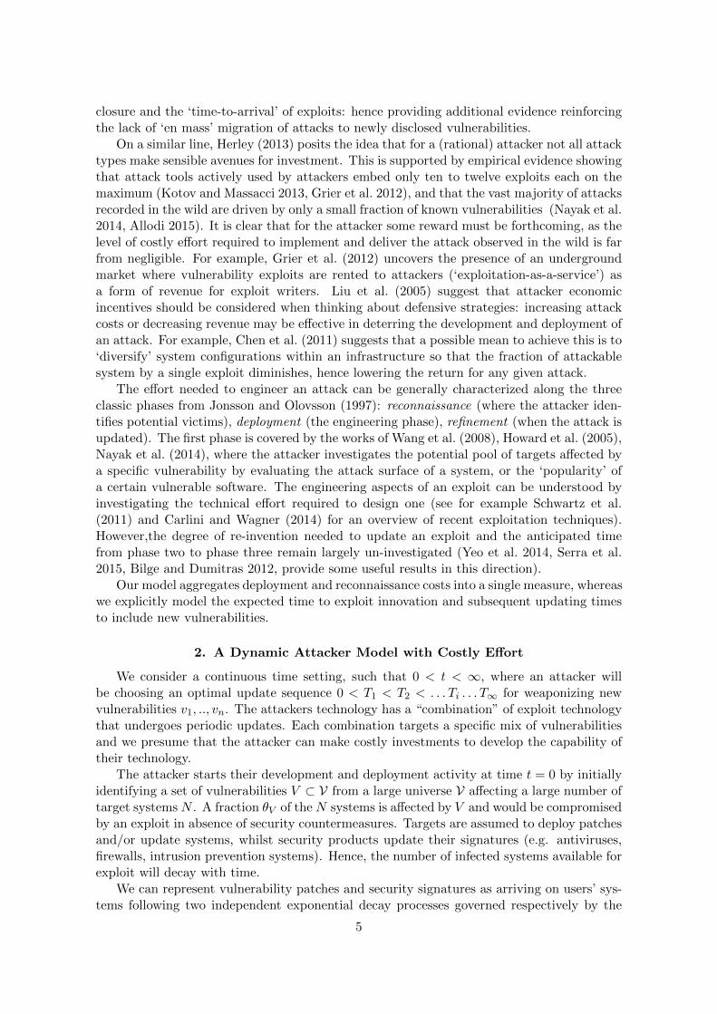
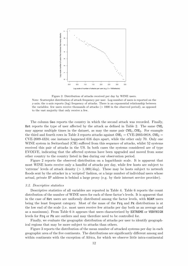
Figure 2: Distribution of attacks received per day by WINE users.
Note: Scatterplot distribution of attack frequency per user. Log-number of users is reported on they-axis; the x-axis reports (log) frequency of attacks. There is an exponential relationship betweenthe variables: few users receive thousands of attacks (> 1000 in the observed period), as opposedto the vast majority that only receive a few.
The column Geo reports the country in which the second attack was recorded. Finally,Hst reports the type of user affected by the attack as defined in Table 2. The same CVEimay appear multiple times in the dataset, as may the same pair CVE1, CVE2. For examplethe third and fourth rows in Table 3 reports attacks against CVE1 = CVE-2003-0818, CVE2 =CVE-2009-4324; one instance happened 616 days apart, while the other only 70. Only oneWINE system in Switzerland (CH) suffered from this sequence of attacks, whilst 52 systemsreceived this pair of attacks in the US. In both cases the systems considered are of typeEVOLVE, indicating that the affected systems have been upgraded and moved from someother country to the country listed in Geo during our observation period.
Figure 2 reports the observed distribution on a logarithmic scale. It is apparent thatmost WINE hosts receive only a handful of attacks per day, while few hosts are subject to‘extreme’ levels of attack density (> 1, 000/day). These may be hosts subject to networkfloods sent by the attacker in a ‘scripted’ fashion, or a large number of individual users whoseactual, private IP address is behind a large proxy (e.g. by their internet service provider).
3.2. Descriptive statistics
Descriptive statistics of all variables are reported in Table 4. Table 6 reports the countdistribution of the number of WINE users for each of these factor’s levels. It is apparent thatin the case of Hst users are uniformly distributed among the factor levels, with ROAM usersbeing the least frequent category. Most of the mass of the Frq and Pk distributions is atthe low end of the scale (i.e. most users receive few attacks per day both as an average andas a maximum). From Table 6 it appears that users characterized by EXTREME or VERYHIGHlevels for Frq or Pk are outliers and may therefore need to be controlled for.
Finally, we evaluate the geographic distribution of attacks per user to identify geograph-ical regions that may be more subject to attacks than others.
Figure 3 reports the distribution of the mean number of attacked systems per day in eachgeographic area of the five continents. The distributions are significantly different among andwithin continents with the exception of Africa, for which we observe little intra-continental
12

Table 4: Descriptive statistics of variables for T , N , U , Hst, Frq, Pk, Geo.
Variable Mean St. dev. Obs. Variable Mean St. dev. Obs.
Delay, Volume, Machines Geo
T 0.99 0.831 2.57E+06 Australia & New Zeal. 0.039 0.194 1.01E+05N 13.552 102.28 2.57E+06 Caribbean 0.013 0.113 33,011U 11.965 93.11 2.57E+06 Central America 0.007 0.084 18,078
Central Asia 0 0.005 63Hst Eastern Africa 0.001 0.026 1,733EVOLVE 0.552 0.497 1.42E+06 Eastern Asia 0.043 0.202 1.09E+05ROAM 0.109 0.312 2.80E+05 Eastern Europe 0.011 0.104 28,277STABLE 0.076 0.265 1.95E+05 Melanesia 0 0.008 159UPGRADE 0.263 0.441 6.77E+05 Micronesia 0.001 0.035 3,123
Middle Africa 0 0.007 112Frq Not Avail. 0.112 0.316 2.89E+05EXTREME 0.004 0.063 10,099 Northern Africa 0.002 0.04 4,088HIGH 0.179 0.384 4.61E+05 Northern America 0.468 0.499 1.20E+06LOW 0.436 0.496 1.12E+06 Northern Europe 0.023 0.151 60,009MEDIUM 0.379 0.485 9.75E+05 Polynesia 0 0.003 28VERYHIGH 0.001 0.037 3,572 South America 0.008 0.09 20,794
South-Eastern Asia 0.023 0.15 59326Pk Southern Africa 0 0.02 1031EXTREME 0 0.011 292 Southern Asia 0.013 0.114 33,901HIGH 0.296 0.456 7.60E+05 Southern Europe 0.063 0.242 1.61E+05LOW 0.091 0.288 2.35E+05 Western Africa 0.001 0.034 2,960MEDIUM 0.609 0.488 1.57E+06 Western Asia 0.018 0.134 46,830VERYHIGH 0.004 0.063 10,182 Western Europe 0.154 0.361 3.95E+05
Table 5: Descriptive statistics for CVE1 and CVE2 variables.
CVE1 CVE2Variable Mean St. dev. Obs. Variable Mean St. dev. Obs.ComplCV E1,H 0.009 0.094 22,769 ComplCV E2,H 0.009 0.096 23,803
ComplCV E1,L 0.42 0.494 1.08E+06 ComplCV E2,L 0.334 0.472 8.58E+05
ComplCV E1,M 0.571 0.495 1.47E+06 ComplCV E2,M 0.657 0.475 1.69E+06
ImpCV E1 9.549 1.417 2.57E+06 ImpCV E2 9.681 1.37 2.57E+06Internet Explorer 0.096 0.295 2.47E+05 Internet Explorer 0.04 0.196 1.03E+05PLUGIN 0.791 0.407 2.03E+06 PLUGIN 0.9 0.3 2.31E+06PROD 0.083 0.276 2.13E+05 PROD 0.037 0.189 95,404SERVER 0.03 0.171 77,507 SERVER 0.023 0.149 58,634Pub. Year 2008.8 2.231 2.57E+06 Pub. Year 2009.4 2.131 2.57E+06
variance. The highest mean arrival of attacks per day is registered in Northern America, Asiaand throughout Europe with the exception of Southern Europe. The mapping of countryand region is defined as in the World Bank Development Indicators.8
4. Empirical Analysis
The data in our sample is quite obviously unique and hence prior to conducting anycorrelative analysis we illustrate some scenarios that provide prima facie statistical evidenceon the validity of the hypotheses identified from our theoretical model.
In accordance with Hypothesis 1 the attacker should prefer to (a) attack the same vul-nerability multiple times rather than for only a short period of time, and (b) create a newexploit only when they want to attack a new software version.
To evaluate these scenarios we identify three types of attack pairs that are summarized inTable 7: in the first type of attack pair (A1) the first attacks and the second attack affect the
8See http://data.worldbank.org/country for a full categorization and breakdown.
13

Table 6: Number of WINE users in the Hst, Frq, and Pk control groups.
Hst #Users Frq #Users Pk #Users
STABLE 1,446,020 LOW 3,210,465 LOW 2,559,819ROAM 96589 MEDIUM 311,929 MEDIUM 983,221UPGRADE 306,856 HIGH 19,683 HIGH 3,783EVOLVE 1,697,570 VERYHIGH 3,919 VERYHIGH 170
EXTREME 1,039 EXTREME 42
Africa
0.00
0.25
0.50
0.75
0 2 4 6 8Log of mean attacks/day by country
Fre
quen
cy
Eastern Africa
Middle Africa
Northern Africa
Southern Africa
Western Africa
Americas
0.00
0.25
0.50
0.75
1.00
0 2 4 6 8Log of mean attacks/day by country
Fre
quen
cy
Caribbean
Central America
Northern America
South America
Asia
0
2
4
0 2 4 6 8Log of mean attacks/day by country
Fre
quen
cy
Central Asia
Eastern Asia
South−Eastern Asia
Southern Asia
Western Asia
Europe
0.0
0.1
0.2
0.3
0.4
0 2 4 6 8Log of mean attacks/day by country
Fre
quen
cy
Eastern Europe
Northern Europe
Southern Europe
Western Europe
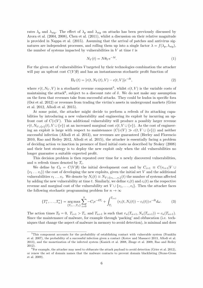
Figure 3: Distribution of attacks per day received in different geographic regions.
Note: Kernel density of mean cumulative attacks per day by geographical region. Regions inAmericas, Asia, and Europe show the highest rates of attacks. Attack densities vary can varysubstantially per region. Oceania is not reported because it accounts for a negligible fraction ofattacks overall.
same vulnerability and, consequently, the same software version; in the second pair (A2) thefirst attack and the second attack affect the same software, but different CVEs and differentsoftware versions; finally the first and second attacks affect the same software and the sameversion but exploit different vulnerabilities (A3). According to our hypothesis we expectthat A1 should be more popular than A2 (in particular when the delay between the attacksis small) whilst A3 should be the least popular of the three.
To evaluate these attacks it is important to consider that users have diverging models ofsoftware security (Wash 2010), different software have different update patterns and updatefrequencies (Nappa et al. 2015), and different attack vectors (Provos et al. 2008).
For example, an attack against a browser may only require the user to visit a webpage,while an attack against a word processing application may need the user to actively opena file on the system (see also the definition of the Attack Vector metric in the CVSSstandard CVSS-SIG (2015)). As these clearly require a different attack process, we furtherclassify Sw in four categories: SERVER, PLUGIN, PROD(-ductivity) and Internet Explorer.The categories are defined by the software names in the database. For example SERVERenvironments are typically better maintained than ‘consumer’ environments and are oftenprotected by perimetric defenses such as firewalls or IDSs. This may in turn affect anattacker’s attitude toward developing new exploits. This may require the attacker to engineerdifferent attacks for the same software version in order to evade the additional mitigatingcontrols in place. Hence we expect the difference between A2 and A3 to be narrower for theSERVER category.
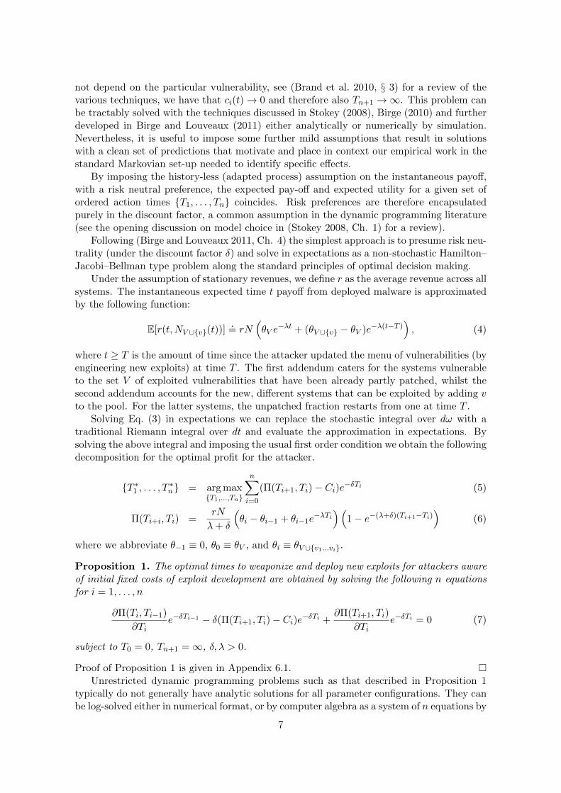
Figure 4 reports a fitted curve of targeted machines as a function of time by software
14
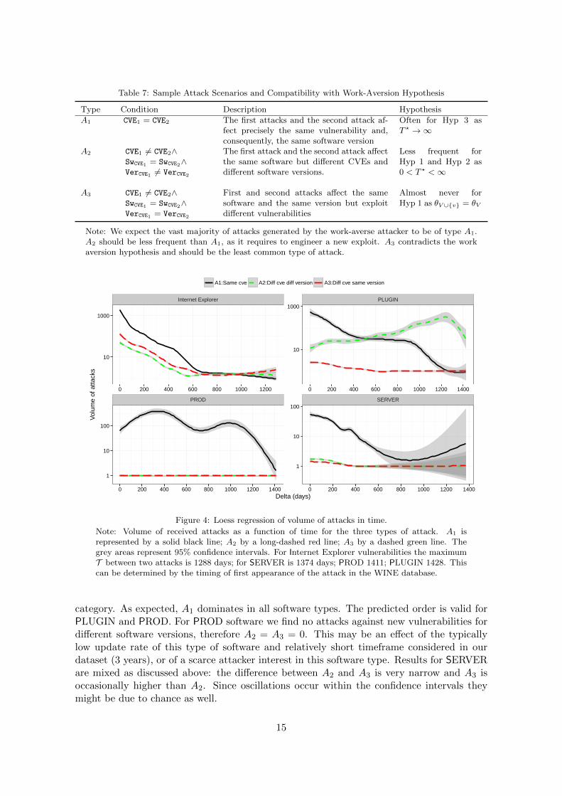
Table 7: Sample Attack Scenarios and Compatibility with Work-Aversion Hypothesis
Type Condition Description Hypothesis
A1 CVE1 = CVE2 The first attacks and the second attack af-fect precisely the same vulnerability and,consequently, the same software version
Often for Hyp 3 asT ? →∞
A2 CVE1 6= CVE2∧SwCVE1 = SwCVE2∧VerCVE1 6= VerCVE2
The first attack and the second attack affectthe same software but different CVEs anddifferent software versions.
Less frequent forHyp 1 and Hyp 2 as0 < T ? <∞
A3 CVE1 6= CVE2∧SwCVE1 = SwCVE2∧VerCVE1 = VerCVE2
First and second attacks affect the samesoftware and the same version but exploitdifferent vulnerabilities
Almost never forHyp 1 as θV ∪{v} = θV
Note: We expect the vast majority of attacks generated by the work-averse attacker to be of type A1.A2 should be less frequent than A1, as it requires to engineer a new exploit. A3 contradicts the workaversion hypothesis and should be the least common type of attack.
Internet Explorer PLUGIN
PROD SERVER
10
1000
10
1000
1
10
100
1
10
100
0 200 400 600 800 1000 1200 0 200 400 600 800 1000 1200 1400
0 200 400 600 800 1000 1200 1400 0 200 400 600 800 1000 1200 1400Delta (days)
Vol
ume
of a
ttack
s
A1:Same cve A2:Diff cve diff version A3:Diff cve same version
Figure 4: Loess regression of volume of attacks in time.
Note: Volume of received attacks as a function of time for the three types of attack. A1 isrepresented by a solid black line; A2 by a long-dashed red line; A3 by a dashed green line. Thegrey areas represent 95% confidence intervals. For Internet Explorer vulnerabilities the maximumT between two attacks is 1288 days; for SERVER is 1374 days; PROD 1411; PLUGIN 1428. Thiscan be determined by the timing of first appearance of the attack in the WINE database.
category. As expected, A1 dominates in all software types. The predicted order is valid forPLUGIN and PROD. For PROD software we find no attacks against new vulnerabilities fordifferent software versions, therefore A2 = A3 = 0. This may be an effect of the typicallylow update rate of this type of software and relatively short timeframe considered in ourdataset (3 years), or of a scarce attacker interest in this software type. Results for SERVERare mixed as discussed above: the difference between A2 and A3 is very narrow and A3 isoccasionally higher than A2. Since oscillations occur within the confidence intervals theymight be due to chance as well.
15

Internet Explorer. is an interesting case in itself. Here, contrary to our prediction, A3 ishigher than A2. By further investigating the data, we find that the reversed trend is ex-plained by one single outlier pair: CVE1 =CVE-2010-0806 and CVE2 =CVE-2009-3672. Thesevulnerabilities affect Internet Explorer version 7 and have been disclosed 98 days apart,within our 120 days threshold. More interestingly, they are very similar: they both affect amemory corruption bug in Internet Explorer 7 that allows for an heap-spray attack resultingin arbitrary code execution. Two observations are particularly interesting to make:
1. Heap spray attacks are unreliable attacks that may result in a significant drop inexploitation success. This is reflected in the Access Complexity:Medium assessmentassigned to both vulnerabilities by the CVSS v2 framework. In our model, this wouldreflected in a lower return r(t,NV (t), V ) for the attacker, as the unreliable exploit mayyield control of fewer machines than those that are vulnerable.
2. The exploitation code found on Exploit-DB9 is essentially the same for these twovulnerabilities. The code for CVE2 is effectively a rearrangement of the code for CVE1,with different variable names. In our model, this would indicate that the cost C(v|V ) ≈0 to build an exploit for the second vulnerability is negligible, as most of the exploitationcode can be re-used from CVE1.
Hence, this vulnerability pair is only an apparent exception: the very nature of the secondexploit for Internet Explorer 7 is coherent with our model and in line with Hyp. 1 and Hyp. 2.Removing the pair from the data confirms the order of attack scenarios identified in Table 7.
We now check how the trends of attacks against a software change with time. Hyp. 3states that the exploitation of the same vulnerability persists in time and decreases slowly ata pace depending on users’ update behaviour. This hypothesis offers an alternative behaviorwith respect to other models in literature where new exploits arrive very quickly after thedate of disclosure, and attacks increase following a steep curve as discussed by Arora et al.(2004).
4.1. An Econometric Model of the Engineering of Exploits
We can use Proposition 2 to identify a number of additional hypothesis that are useful toformulate the regression equation. At first we notice that T ? = O(log(θv−θV )N). Thereforewe have a first identification relation between the empirical variable U (corresponding to N)and the empirical variable T (whose correspondence to T ? is outlined later in this section).
Hypothesis 4. There is a log-linear relation between the number of attacked systems Uand the delay T .
Since ∂T ?/∂((θv−θV )N) < 0 a larger number of attacked systems U on different versions(θv 6= θV ) would imply a lower delay T (as there is an attractive number of new systemsthat guarantee the profitability of new attacks). In contrast, the baseline rate of attacksimpacts negatively the optimal time T as ∂T ?/∂(θVN) > 0 since a larger pool of vulnerablemachines makes it more profitable to continue with existing attacks (as per Hyp. 1).
Hypothesis 5. The possibility of launching a large number of attacks against systems forwhich an exploit already exists lengthens the time for weaponizing a vulnerability (N ·(Ver0 =Verv) ↑ =⇒ T ↑), whereas an increase in potential attacks on different systems is anincentive towards a shorter weaponization cycle (N · (Ver0 6= Verv) ↑ =⇒ T ↓).
9See Exploit-DB (http://www.exploit-db.com, last accessed January 15, 2017.), which is a public datasetfor vulnerability proof-of-concept exploits. CVE1 corresponds to exploit 16547 and CVE2 corresponds to exploit11683.
16

N(ΘV ∪{v},∆) =∫∞
max{∆,T ∗} min{N(ΘV , t−∆,∆), N(ΘV ∪{v}, t,∆)}dt
At T ∗ Attacker deploys vulnerability v
ΘV ∪{v}N →
N(ΘV ∪{v}, t,∆) ← ΘV ∪{v}Ne−λ(t−T ∗)
New attacks on v after ∆↓ΘVNe−λ(t−∆)
Attempted attacks on v0 ∈ V
T ∗t−∆ ≥ 0 t ≥ T ∗
∆
Figure 5: Computing the delay (T ) against different vulnerabilities.
Note: Change in the number of attacked systems for two attacks against different systems ∆ =T days apart. The first attack happens at t − T ≥ 0 and the number of attacked systemsU(ΘV ∪ {v}, t, T ) is derived from Eq. (1) as ΘVNe
−λ(t−T ). The number of systems attacked bythe new exploit introduced at T ? is derived as U(ΘV ∪{v}, t, T
?) = NΘV ∪{v}e−λ(t−T?)dt.
When considering the effects of costs, we observe that, as ∂T ?/∂C(v|V ) > 0, the presenceof a vulnerability with a low attack complexity implies dC(v|V ) < 0, and therefore reflectsa drop in the delay T between the two attacks. We have already discussed this possibilityas Hypothesis 2.
As for revenues, it is ∂T ?/∂r < 0 so that an higher expected profit would imply a shortertime to weaponization. However, we cannot exactly capture the latter condition since in ourmodel the actual revenue r is stationary and depends only on the captured machine ratherthan the individual type of exploit. A possible proxy is available through the Imp variable,but it only shows the level of technical compromise that is possible to achieve. Unfortunately,such information might not correspond to the actual revenue that can be extracted by theattacker. For example, vulnerabilities that only compromise the availability of a system arescored low according to the CVSS standard. However, for an hacker offering “booter services”to on- line gamers (i.e. DDoS targeted attack against competitors) these vulnerabilities arethe only interesting source of revenues Hutchings and Clayton (2016).
However Imp can also be seen as a potential conditional factor to boost the attractivenessof a vulnerability as the additional costs of introducing an exploit might be justified by theincreased capability to produce more havoc.
Hypothesis 6. Vulnerabilities with higher impact increase revenue and therefore decreasenumber of attacks (ImpCVE2 > ImpCVE1 =⇒ U ↓).
As the time of introduction of an exploit T ? can not be directly measured from ourdataset, we use T (i.e. the time in between two consequent attacks) as a proxy for thesame variable. Figure 5 reports a pictorial representation of the transformation. Eachcurve represents the decay in time of number of attacks against two different vulnerabilities.The first attack (blue line) is introduced at t = 0, and the second (red line) at t = T ?.
17
The number of received attacks is described by the area below the curve within a certaininterval. Let U(ΘV ∪ {v}, t, T ) represent the number of systems that receive two attacks Tdays apart, at times t − T and t respectively. Depending on the relative position of t − Twith respect to T ?, the interval within which reside the measured attacks on the pair ofvulnerabilities will be
∫∞max(T ?,T ) U(·)dt. Setting the number of attacks at time t − T as
U(θv, t − T ) = Nθve−λ(t−T ) and the attacks received on the second vulnerability at time t
as U(θV ∪{v}, t) = NθV ∪{v}e−λ(t−T ?), we obtain
U(θV ∪{v}, t, T ) = min(Nθve
λT ), NθV ∪{v}eλT ?)∫ ∞
max(T ,T ?)e−λtdt (9)
Solving for the two cases T ? > T and T ? < T , we formulate the following claim:
Claim 1.
logU(θV ∪{v}, t, T ) =
{log N
λ − λT? + λT + log θv if T ? > T
log Nλ + λT ? − λT + log θV ∪{v} if T ? < T
(10)
The sign of the coefficient for T oscillates from positive to negative as T increases.
Proof of Claim 1 and its empirical evaluation are given in Appendix 6.4. �Reviewing Figure 1, our data suggests that T is on average more than 100 days with
respect to T ?. Therefore we have:
logU = −λT + λT ? + logN
λ+ log θV ∪{v}
Substituting T ? from Eq. (8), the number of expected attacked systems after T days is:
logU = −λT + λ
[1
δlog
(C(v|V )
r− δ
λ+ δ(θV ∪{v} − θV )N
)]+ log
N
λ+ log θV ∪{v} (11)
Our regression model tests the hypotheses above by reflecting the formulation provided inEq. (11). T can be measured directly in our dataset; the cost of development of an exploitsC(v|V ) can be estimated by the proxy variables ComplCVE2 , as the complexity associated withexploit development requires additional engineering effort (and is thus related to an increasein development effort) CVSS-SIG (2015). We can not directly measure the revenue r andthe number of systems N affected by the vulnerability, but we can estimate the effect ofan attack on a population of users by measuring the impact (Imp) of that vulnerability onthe system: higher impact vulnerabilities (i.e. (ImpCV E2 > ImpCV E1) allow the attacker tocontrol a higher fraction of the vulnerable system, and therefore extract higher revenue r fromthe attack. Similarly, the introduction of an attack with a higher impact can approximatethe difference in attack penetration (θV ∪{v} − θV )N for the new set of exploits as it allowsthe attacker for a higher degree of control on the affected systems. Finally, high impactvulnerabilities (ImpCV E2,H), for example allowing remote execution of arbitrary code onthe victim system, leave the ΘV ∪{v}N systems under complete control of the attacker; incontrast, a low impact vulnerability, for example causing a denial of service, would allow foronly a temporary effect on the machine and therefore a lower degree of control. In Table 8we report the sample correlation matrix for the variables included in the regression systemwe will use to parameterize the model, from an econometric standpoint, the highest pairwisecorrelations with Ti are Frq MEDIUM and Pk HIGH, however these have correlations of lessthan 20%, as such the standard issues on rank and collinearity are not present.
18

Table 8: Correlation Matrix of All Variables Included in the Model.
Model variable 1. 2. 3. 4. 5. 6. 7. 8. 9. 10. 11.1. T 12. ComplCV E2L -0.130 13. ImpCV E2H 0.058 -0.237 14. ImpCV E2 > ImpCV E1 0.092 -0.097 0.055 15. Geo North. Am. 0.020 0.146 -0.040 -0.035 16. Geo Western Eu. 0.022 -0.026 0.011 -0.051 -0.410 17. Hst EVOLVE -0.084 0.024 -0.065 0.022 -0.057 0.015 18. Hst UPGRADE 0.054 0.004 0.030 -0.017 0.084 -0.042 -0.656 19. Frq HIGH 0.104 -0.050 0.052 0.107 0.087 -0.183 -0.225 -0.024 110. Frq MEDIUM 0.136 0.077 -0.103 0.127 0.014 0.096 -0.087 0.186 -0.369 111. Pk HIGH 0.166 -0.008 0.045 0.049 0.020 0.033 -0.288 0.034 0.678 0.052 112. Pk MEDIUM -0.087 0.031 -0.054 -0.004 -0.023 -0.008 0.197 0.004 -0.549 0.101 -0.814
Table 9: Summary of predictions derived from the model.
Model variable Regressor Expectation Hyp. RationaleT T β1 < 0 Hyp. 3, Hyp. 4, Hyp. 5 Shorter exploitation times
are associated with morevulnerable systems, henceT ↑ =⇒ U ↓.
C(V |v) ComplCV E2,L β2 < 0 Hyp. 1, Hyp. 5, Hyp. 2 The introduction of a newreliable, low-complexity ex-ploit minimizes implementa-tion costs, thus C ↓ =⇒U ↓.
θV ∪{v} ImpCV E2,H β3 > 0 Hyp. 6, Hyp. 5 High impact vulnerabilitiesallow the attacker for a com-plete control of the attackedsystems, hence θV ∪{v} ↑=⇒ U ↑.
r, (θV ∪{v} − θV ) ImpCV E2 > ImpCV E1 β4 < 0 Hyp. 6 Selecting a higher impactexploit for a new vulnera-bility increases the expectedrevenue and increases thefraction of newly controlledsystems with respect to theold vulnerability. r ↑ =⇒U ↓ and (θV ∪{v}−θV ) ↑ =⇒U ↓.
To test our hypotheses, we set three equations to evaluate the effect of our regressors onthe dependent variable. The formulation is derived from prime principles from Eq. (11) asdiscussed above. Our equations are:
Model 1: log(Ui) = β0 + β1Ti + εi (12)
Model 2: log(Ui) = · · ·+ β2Compli,CV E2,L + εi (13)
Model 3: log(Ui) = · · ·+ β3Impi,CV E2,H + β4(Impi,CV E2 > Impi,CV E1)εi (14)
Where i indexes the pair of attacks received by each machine after T days, Compli,CV E2,L
indicates that CVE2 has a low complexity, and Impi,CV E2,H indicates that CVE2 has a High (≥7) impact. Both classifications for Compl and Imp are reported by the CVSS standardspecification. The correlation matrix of the model variables is reported in Table 8.
The mapping of each term with our hypotheses and the predicted values of the regressorsare described in the Table 9. Further, we add the vector of controls Z to the regression toaccount for exogenous factors that may confound the observation, as discussed in Section 3.2:
19
-0.6
Northern America
1
-0.4
-0.2
0
1
0.2
Western Europe
PC
3 -
Expla
in 9
% o
f G
eo v
ariance
0.5
0.4
Principal Components of Geo-location
0.6
PC2 - Explain 23% of Geo variance
0.5
0.8
Northern Europe
PC1 - Explain 55% of Geo variance
1
0
Eastern EuropeSouthern Asia
0
-0.5 -0.5
Eastern Asia
evol:EVOLVE
-0.4
peak:MEDIUM
1
-0.2
0
0.2
0.5 0.6
freq:EXTREME
PC
3 -
Exp
lain
17
% v
aria
nce
0.4
evol:ROAM
freq:VERYHIGH
0.4
freq:HIGH
peak:EXTREME
0.6
Principal Components of Users
peak:VERYHIGH
PC2 - Explain 26% variance
0 0.2
0.8
PC1 - Explain 37% variance
0
evol:UPGRADE
1
-0.5 -0.2
peak:HIGH
freq:MEDIUM
-0.4-1 -0.6
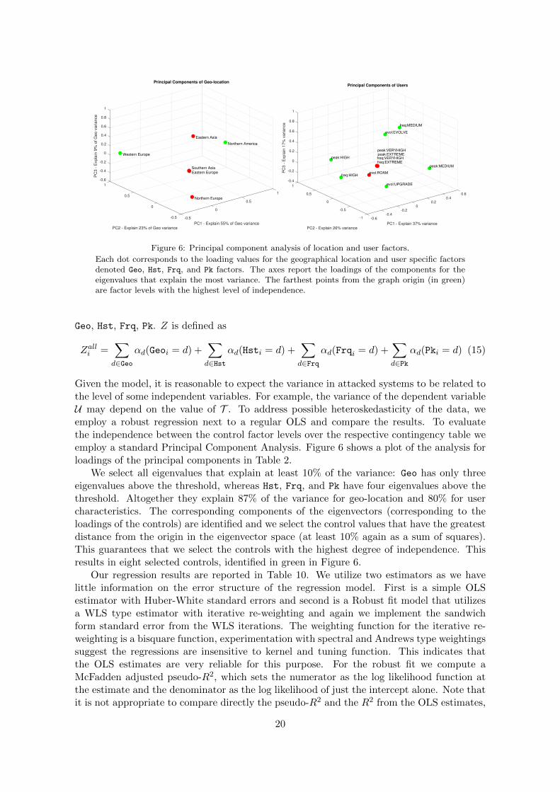
Figure 6: Principal component analysis of location and user factors.
Each dot corresponds to the loading values for the geographical location and user specific factorsdenoted Geo, Hst, Frq, and Pk factors. The axes report the loadings of the components for theeigenvalues that explain the most variance. The farthest points from the graph origin (in green)are factor levels with the highest level of independence.
Geo, Hst, Frq, Pk. Z is defined as
Zalli =∑d∈Geo
αd(Geoi = d) +∑d∈Hst
αd(Hsti = d) +∑d∈Frq
αd(Frqi = d) +∑d∈Pk
αd(Pki = d) (15)
Given the model, it is reasonable to expect the variance in attacked systems to be related tothe level of some independent variables. For example, the variance of the dependent variableU may depend on the value of T . To address possible heteroskedasticity of the data, weemploy a robust regression next to a regular OLS and compare the results. To evaluatethe independence between the control factor levels over the respective contingency table weemploy a standard Principal Component Analysis. Figure 6 shows a plot of the analysis forloadings of the principal components in Table 2.
We select all eigenvalues that explain at least 10% of the variance: Geo has only threeeigenvalues above the threshold, whereas Hst, Frq, and Pk have four eigenvalues above thethreshold. Altogether they explain 87% of the variance for geo-location and 80% for usercharacteristics. The corresponding components of the eigenvectors (corresponding to theloadings of the controls) are identified and we select the control values that have the greatestdistance from the origin in the eigenvector space (at least 10% again as a sum of squares).This guarantees that we select the controls with the highest degree of independence. Thisresults in eight selected controls, identified in green in Figure 6.
Our regression results are reported in Table 10. We utilize two estimators as we havelittle information on the error structure of the regression model. First is a simple OLSestimator with Huber-White standard errors and second is a Robust fit model that utilizesa WLS type estimator with iterative re-weighting and again we implement the sandwichform standard error from the WLS iterations. The weighting function for the iterative re-weighting is a bisquare function, experimentation with spectral and Andrews type weightingssuggest the regressions are insensitive to kernel and tuning function. This indicates thatthe OLS estimates are very reliable for this purpose. For the robust fit we compute aMcFadden adjusted pseudo-R2, which sets the numerator as the log likelihood function atthe estimate and the denominator as the log likelihood of just the intercept alone. Note thatit is not appropriate to compare directly the pseudo-R2 and the R2 from the OLS estimates,
20

which suggests that the model captures roughly 10% of the variation in numbers of attackedmachines, as opposed to explaining 35% of the model likelihood for the pseudo-R2.
The set of OLS and Robust regressions returns very similar estimations. The introductionof the controls only change the sign of β1 from positive to negative for Model 1. This mayindicate that the type of user is a significant factor in determining the number of deliveredattacks, which is consistent with previous findings Nappa et al. (2015). Interestingly, thefactor that introduces the highest change in the estimated coefficient β1 for T is Compl (Model2), whereas its estimate remains essentially unchanged in Model 3. This may indicate thatthe cost of introduction of an exploit has a direct impact on the time of delivery of the exploit.The coefficients for all other regressors are consistent across models, and their magnitudechanges only slightly with the introduction of the controls. This should be expected: usercharacteristics should not influence the characteristics of the vulnerabilities present on thesystem. Hence, the distribution of attacks in the wild seems to be prevalently dependent onsystem characteristics and independent of user type. The signs of the coefficients for the Imp
variables suggest that both the impact of a vulnerability and the relation of the impact ofthe new vulnerability w.r.t. previous ones have an effect on the number of attacked systems.Interestingly, a high impact encourages the deployment of attacks and increases the numberof attacked systems, whereas the introduction of a higher impact vulnerability requires theinfection of a smaller number of systems as revenues extracted from each machine increase.This indicates that when introducing a new exploit, the attacker will preferably choose onethat grants a higher control over the population of users (θV ∪{v} > θV ) and use it against alarge number of system. This goes in the same direction of recent findings that suggest thatvulnerability severity alone is not a good predictor for exploitation in the wild Allodi andMassacci (2014), Bozorgi et al. (2010), and that other factors such as software popularity ormarket share may play a role Nayak et al. (2014).
5. Discussion, Conclusions and Implications
This paper implements a model of the Work-Averse Attacker as a new conceptual framingto understand cyber threats. Our model presumes that an attacker is a resource-limited actorwith fixed costs that has to choose which vulnerabilities to exploit to attack the ‘mass ofInternet systems’. Work aversion simply means that effort for the attacker is costly (interms of cognition and opportunity costs), hence a trade-off exists between effort exerted onnew attacking technologies and the anticipated reward schedule from these technologies. Astechnology combinations mature, their revenue streams are presumed dwindle.
In this framework, an utility-maximizing attacker will drive exploit production accordingto their expectations that the newly engineered attack will increase net profits from attacksagainst the general population of internet users. As systems in the wild get patched unevenlyand often slowly in time (Nappa et al. 2015), we model the production of new vulnerabilityexploits following Stokey’s ‘economy of inaction’ logic, whereby ‘doing nothing’ before acertain (time) threshold is the best strategy. From the model a cost constraint driving theattacker’s exploit selection strategy naturally emerges. In particular, we find theoretical andempirical evidence for the following:
1. An attacker massively deploys only one exploit per software version. The only exceptionwe find is for Internet Explorer; the exception is characterised by a very low cost tocreate an additional exploit, where it is sufficient to essentially copy and paste codefrom the old exploit, with only few modifications, to obtain the new one. This findingsupports Hyp. 1.
21

Table
10:
Ord
inary
Lea
stSquare
sand
Robust
Reg
ress
ion
Res
ult
s
DependentVariable:natu
rallogarith
mofth
enumberofattacked
machin
eslog(U
i)
Model1
Model2
Model3
OLS
Robust
OLS
Robust
OLS
Robust
Z1:Z8
Z1:Z8
Z1:Z8
Z1:Z8
Z1:Z8
Z1:Z8
c0.927
0.006
0.731
0.096
1.065
0.122
0.845
0.171
0.933
-0.106
0.783
0.039
(0.001)
(0.003)
(0.001)
(0.003)
(0.001)
(0.003)
(0.001)
(0.003)
(0.004)
(0.005)
(0.003)
(0.004)
T0.018
-0.051
0.012
-0.044
-0.006
-0.092
-0.003
-0.071
-0.005
-0.091
-0.004
-0.071
(0.001)
(0.001)
(0.001)
(0.001)
(0.001)
(0.001)
(0.001)
(0.001)
(0.001)
(0.001)
(0.001)
(0.001)
ComplC
VE
2L
-0.326
-0.479
-0.228
-0.324
-0.313
-0.464
-0.22
-0.314
(0.002)
(0.002)
(0.001)
(0.001)
(0.002)
(0.002)
(0.001)
(0.001)
ImpC
VE
2H
0.144
0.236
0.063
0.131
(0.003)
(0.003)
(0.003)
(0.003)
ImpC
VE
2>
ImpC
VE
1-0
.088
-0.209
0.012
-0.087
(0.003)
(0.003)
(0.002)
(0.002)
Z1:GeoNorth.Amer.
0.604
0.37
0.679
0.422
0.671
0.419
(0.002)
(0.001)
(0.002)
(0.001)
(0.002)
(0.001)
Z2:GeoW
est.Eu.
0.155
0.105
0.17
0.116
0.163
0.114
(0.002)
(0.002)
(0.002)
(0.002)
(0.002)
(0.002)
Z3:HstEVOLVE
0.191
0.129
0.208
0.141
0.223
0.149
(0.002)
(0.002)
(0.002)
(0.002)
(0.002)
(0.002)
Z4:HstUPGRADE
0.112
0.072
0.116
0.076
0.113
0.075
(0.002)
(0.002)
(0.002)
(0.002)
(0.002)
(0.002)
Z5:FrqHIG
H0.24
0.147
0.212
0.127
0.279
0.157
(0.003)
(0.003)
(0.003)
(0.003)
(0.003)
(0.003)
Z6:FrqM
EDIU
M0.328
0.227
0.358
0.246
0.41
0.271
(0.002)
(0.002)
(0.002)
(0.002)
(0.002)
(0.002)
Z7:PkHIG
H0.513
0.442
0.567
0.49
0.531
0.477
(0.004)
(0.003)
(0.004)
(0.003)
(0.004)
(0.003)
Z8:PkM
EDIU
M0.379
0.274
0.412
0.299
0.411
0.301
(0.003)
(0.002)
(0.003)
(0.002)
(0.003)
(0.002)
PseudoR
2-
-0.326
0.341
--
0.331
0.347
--
0.331
0.347
R2
0.00
0.093
--
0.016
0.126
--
0.017
0.13
--
F348.661
26,551.467
--
18,548.248
33,422.784
--
9,989.879
28,915.597
--
Obs.
2,324,500
2,324,500
2,324,500
2,324,500
2,324,500
2,324,500
2,324,500
2,324,500
2,324,500
2,324,500
2,324,500
2,324,500
Mod
el1:
log(Ui)
=β0
+β1T i
+ε i
Mod
el2:
log(Ui)
=β0
+β1T i
+β2Compli,CVE2,L
+ε i
Mod
el3:
log(Ui)
=β0
+β1T i
+β2Compli,CVE2,L
+β3Impi,CVE2,H
+β4Impi,CVE2>
Impi,CVE1ε i
Notes:
Th
eth
ree
mod
eleq
uati
on
sre
flec
tth
ed
efin
itio
nof
the
exp
ecte
d(l
og)
nu
mb
erof
aff
ecte
dm
ach
ines
aft
eran
inte
rvalT
.T
he
regre
ssio
nm
od
elfo
rmu
lati
on
isd
eriv
edfr
om
pri
me
pri
nci
ple
from
Eq.
11.
Th
eex
pec
ted
coeffi
cien
tsi
gn
sare
giv
enin
Tab
le9.
For
each
mod
elw
eru
nfo
ur
sets
of
regre
ssio
ns.
OL
San
dR
ob
ust
regre
ssio
ns
are
pro
vid
edto
ad
dre
sses
het
erosc
edast
icit
yin
the
data
.R
2an
dF−statistics
are
rep
ort
edfo
rth
eO
LS
esti
mati
on
s.N
ote
that
the
pse
ud
o-R
2are
com
pu
ted
for
the
rob
ust
regre
ssio
ns,
usi
ng
the
McF
ad
den
ad
just
edap
pro
ach
R2
=1−
(log(LLfull
)−K
)/lo
g(LLint),
wh
ere
log(LLfull
)is
the
log
likel
ihood
for
the
full
mod
elm
inu
sth
enu
mb
erof
slop
ep
ara
met
ersK
ver
sus
the
log
likel
ihood
of
the
inte
rcep
talo
ne
an
dsh
ou
ldn
ot
be
com
pare
dd
irec
tly
toth
eO
LSR
2.
Coeffi
cien
tes
tim
ati
on
sof
the
two
sets
of
regre
ssio
ns
are
con
sist
ent.
All
regre
ssio
ns
are
run
wit
han
dw
ith
ou
tth
ese
tof
contr
ols
defi
ned
by
the
PC
Aan
aly
sis
pic
tori
ally
rep
ort
edin
Fig
.6.
All
coeffi
cien
tsi
gn
sfo
rth
eth
ree
mod
els
refl
ect
the
work
-aver
seatt
ack
erm
od
elp
red
icti
on
s,w
ith
the
on
lyex
cep
tion
of
the
esti
mati
on
forT
wit
hn
oco
ntr
ols
for
wh
ich
the
pre
dic
tion
forβ1
isin
ver
ted
.T
his
may
ind
icate
that
use
rch
ara
cter
isti
csare
rele
vant
fact
ors
for
the
arr
ival
tim
eof
exp
loit
sw
hen
oth
erfa
ctors
rela
ted
toth
esy
stem
are
not
acc
ou
nte
dfo
r.T
he
intr
od
uct
ion
ofCompl
inM
od
el2
sign
ifica
ntl
ych
an
ges
the
esti
mate
forβ1,
wh
erea
sImp
inM
od
el3
leaves
the
esti
mate
sfo
rCompl
an
dT
un
chan
ged
.H
ighImp
vu
lner
ab
ilit
ies
ten
dto
incr
ease
volu
me
of
att
ack
s.W
ere
port
on
lyst
an
dard
erro
rsw
ith
ou
tst
arr
ing
p-v
alu
esas
all
coeffi
cien
tsare
sign
ifica
nt
du
eto
the
nu
mb
erof
ob
serv
ati
on
sin
the
data
set.
All
stan
dard
erro
rsare
esti
mate
du
sin
gth
eH
ub
er-W
hit
eap
pro
ach
.
22

2. Low complexity vulnerabilities for which a reliable exploit can be easily engineeredlower the production costs and favor the deployment of the exploit. This findingsupports Hyp. 2.
3. The attacker deploys new exploits relatively slowly over time, driven by a slowly de-creasing instantaneous profit function; empirically, we find that attacks 1000 days apartare still driven by the same exploits in about 20% of the cases, and that the effect ofthe passage of time in between attacks (T ) on the number of affected system is indeednegative and very small given the current patching rate. This finding supports Hyp. 3and Hyp. 5.
4. The presence of a high impact vulnerability increases the incidence of exploitation inthe wild. Similarly, gaining a higher control over the attacked systems heightens theattacker’s revenue and decreases the number of systems that need to be infected tobalance development costs. This supports Hyp. 6.
The above findings suggest that risk associated with software vulnerabilities can notbe solely measured in terms of technical severity, and that other, measurable factors maybe included in the assessment, as previously suggested by some authors (see for exampleBozorgi et al. 2010, Houmb et al. 2010, Allodi and Massacci 2014). While characteristicsof the attacker and of the user, such as skill or competence, in system security may remainhard to measure, this paper shows how measurable environmental indexes may be used toestimate the economic incentives that exists for the attacker (as suggested, for example, byAnderson 2008).
5.1. Implications For Theory
The modeling of cyber attacks and cyber risk has traditionally been centered on the vul-nerabilities present on systems and their technical severity. In recent years, this perspectivehas been largely questioned as the typically limited attacker resources became empiricallyapparent (Grier et al. 2012), and advances in security modeling started distinguishing be-tween opportunistic (i.e. untargeted) and deliberate (i.e. targeted) attacks (see Ransbothamand Mitra 2009, for a discussion on this). However, current studies modeling cybersecurityevents typically think of the attacker as employing an undefined ‘attack generation func-tion’, which too easily collapses to an ‘all-powerful’ attacker that may generate an attack forwhichever vulnerability exists.
Little theoretical discourse has been developed around the identification of models ofvulnerability exploit production. Most assessments on whether the attacker will be successfulare still produced by means of ‘expert estimates’ (Wang et al. 2008) or ‘technical measures ofvulnerabilities’ (Naaliel et al. 2014) that, however, are known not to correlate with attackerchoices as shown by Bozorgi et al. (2010). Researchers noted that “some vulnerabilities aredifferent than others” (Nayak et al. 2014), but a rationale enabling this distinction betweenvulnerabilities is yet to be fully discussed.
In contrast to the classic ‘all powerful attacker’ model (Dolev and Yao 1983b) thatcan and will exploit potentially any vulnerability, this paper develops the thesis that theutility-maximizing attacker will generally ‘avoid to work’ until the perceived utility of thedeployment of a new attack becomes positive w.r.t. to expectations derived from the previousattack at time T ?. This economic perspective has been previously employed in game-theoreticapproaches (Manshaei et al. 2013), but it typically considers two actors (the organization- namely the defender and the attacker) that react to each other’s strategies. While thisis significant for the case of targeted attacks, where the attacker can observe part or allof the organization’s defenses and the defender chooses a strategy to decrease its attack
23
surface (Howard et al. 2005), it is unclear how this maps to the case of the ‘general attacker’that deploys attacks against the vast Internet population. As the average Internet user haslittle to no knowledge of computer and network security (Wash 2010), they are unlikely todeploy defensive strategies and to react strategically to new attacks. Hence, in this case, theattacker operates in an environment where relevant variables are not entirely exogenouslymanipulated by an intelligent adversary (from the attacker’s perspective, the defender). Thestrategy of the mass of defenders may only be statistically determined.
While untargeted attacks exploiting software vulnerabilities make up for a significantfraction of all attacks recorded (Provos et al. 2008, Baker et al. 2012), this particular settingis largely unexplored in literature. As there is virtually no ‘purely reactive strategy’ to thedecision of the attacker, part of the debate on regulatory intervention may focus on howto devise regulatory models that, on average, will increase the development costs for theattacker. Even targeted attacks require fixed costs and it is unclear whether such attackscould be captured by variation in the work aversion (or by making reward a function of costssuch as reconnaissance) (Verizon 2011, Bilge and Dumitras 2012).
5.2. Implications For Information Security Management and Policy
Our findings suggest that the rationale behind vulnerability exploitation could be lever-aged by defenders to deploy more cost-effective security countermeasures. For example, it iswell known that software updates correspond to an increased risk of service disruption (e.g.for incompatibility problems or updated/deprecated libraries). However, if most of the riskfor a particular software version comes from a specific vulnerability, than countermeasuresother than patching may be more cost-effective. For example, maintaining network IDSsignatures may be in this case a better option than updating the software, because one IDSsignature could get rid of the great majority of risk that characterizes that system while asoftware patch may ‘overdo it’ by fixing more vulnerabilities than necessary.
Further, this view on the attacker has repercussions on the impact of vulnerability disclo-sure in terms of security of the user or organization. Work in this direction explored both theeconomic incentives for sharing information security (Gal-Or and Ghose 2005, Ransbothamet al. 2012) and the impact of vulnerability disclosure on attacks and firm value (Arora et al.2008, Telang and Wattal 2007). Some of this discussion resulted in recent open debatesregarding policies for vulnerability disclosure, and the drafting of ISO standards to guidevulnerability communication to the vendor and to the public (e.g. ISO/IEC 29147:2014).For example, the United States Department of Commerce NTIA forum for vendors, indus-try players, and security researchers to discuss procedures and timings of the vulnerabilitydisclosure process. 10 However, this discussion is not currently guided by a theoreticalframework that can act as a supporting tool for the decision maker. For example, this maybe applied to the case of vulnerability disclosure to evaluate or estimate the effect in terms ofthe effective increase in risk of attacks that follows the disclosure, extending previous workin this same direction by Mitra and Ransbotham (2015).
Further, a more precise and data-grounded understanding of the attacker poses a strategicadvantage for the defender. For example, software diversification and code differentiationhas already been proposed as a possible alternative to vulnerability mitigation (Chen et al.2011, Homescu et al. 2013). By diversifying software the defender effectively decreases thenumber of systems the attacker can compromise with one exploit, effectively making theexistence conditions for Eq. (8) harder to satisfy than by means of a patch release strategy
10The NTIA forum can be found at https://www.ntia.doc.gov/other-publication/2016/
multistakeholder-process-cybersecurity-vulnerabilities, last accessed January 15, 2017.
24

employed by vendors. For example, software vendors may randomize the distribution ofvulnerability patches to their users, to minimize the attacker’s chances of matching theirexploits with the vulnerabilities actually present on the system. A random distribution ofpatches would simply decrease the fraction of attackable systems regardless of the attacker’schoice in which vulnerability to exploit. Moreover, diversifying defenses may be in factless onerous than re-compiling code bases (when possible) or maintaining extremely diverseoperational environments.
5.3. Limitations and Extensions
Our model describes an attacking adversary with costly production of malware. Themodel aims at explaining the attacker’s preference in exploiting one vulnerability over an-other rather than casting a wide net immediately after a new vulnerability has been discov-ered. However, this preference can not be directly measured, but must be inferred throughtheir real attack signatures from a record of attempted security incursions.
Records of attacks detected over a user’s machine are necessarily conditioned over theuser’s proneness in receiving a particular attack. For example, a user may be inclined toopen executable email attachments, but not in visiting suspicious websites. Thus, theremay be a disassociation between the observed attacks and those engineered by the attacker.For our empirical dataset this limitation is mitigated by WINE reporting attack data on avery large representative sample of Internet users (Dumitras and Shou 2011). However, wealso need to have additional conditioning variables to permit identification of the impact onvarious behavioral characteristics. Many of the additional characteristics of users that mayinfluence the observed volume of attacks, such as educational level and culture which, arevery difficult or close to impossible to gauge at the scale of data presented in this paper.As proxies to control for this effect we employ the User Profile, Frequency, Peak andgeographic location variables, as these outline the user’s proneness in receiving attacks.Further, geographic location may not only influence effects related to user culture, but alsoon attack diffusion.
Software versioning information is known to be unreliable at times with respect to vulner-ability existence (Nguyen et al. 2015). Further, software versions can not be easily ‘ordered’throughout software types, as different vendors adopt different naming schemes for softwarereleases (Christey and Martin 2013, for an overview). We can not therefore order softwareversions over time easily. This is however irrelevant to our study as we are interested in mea-suring the sequences of newer attacks received by internet users, as opposed to measuringthe existence of new exploits for subsequent software releases, our model predicts that theattacker will perform this information filtration dynamically as they view the rewards fromtheir activities. A limitation of our empirical dataset is obviously the market penetration ofSymantec, as of 2016 Symantec self reports that it is the largest security vendor11 by marketshare in anti-virus and overall software security and hence has a broad coverage recordingattacks on customers. However, third party verifiable measurement of these claims is difficulthence replication studies with different security vendors would be welcomed and given thesimplicity of our regression specification easily implemented.
References
Allodi, L. (2015). The heavy tails of vulnerability exploitation. In Proceedings of the 2015 EngineeringSecure Software and Systems Conference (ESSoS’15).
11Indeed, according to the 2016 market share Symatec has held this position for the last 15 years, seehttps://www.symantec.com/en/uk/about/newsroom/analyst/reports
25

Allodi, L., M. Corradin, and F. Massacci (2015). Then and now: On the maturity of the cybercrimemarkets the lesson that black-hat marketeers learned. IEEE Transactions on Emerging Topicsin Computing 4 (1), 35–46.
Allodi, L., V. Kotov, and F. Massacci (2013). Malwarelab: Experimentation with cybercrime attacktools. In Proceedings of the 2013 6th Workshop on Cybersecurity Security and Test.
Allodi, L. and F. Massacci (2014, August). Comparing vulnerability severity and exploits usingcase-control studies. ACM Transaction on Information and System Security (TISSEC) 17 (1).
Anderson, R. (2008). Information security economics - and beyond. In Proceedings of the 9th Inter-national Conference on Deontic Logic in Computer Science, DEON ’08, pp. 49–49.
Arora, A., R. Krishnan, A. Nandkumar, R. Telang, and Y. Yang (2004). Impact of vulnerabilitydisclosure and patch availability-an empirical analysis. In Proceedings of the 3rd Workshop onEconomics and Information Security.
Arora, A., R. Telang, and H. Xu (2008). Optimal policy for software vulnerability disclosure. Man-agement Science 54 (4), 642–656.
Asghari, H., M. Van Eeten, A. Arnbak, and N. Van Eijk (2013). Security economics in the httpsvalue chain. In Twelfth Workshop on the Economics of Information Security (WEIS 2013),Washington, DC.
August, T. and T. I. Tunca (2006). Network software security and user incentives. ManagementScience 52 (11), 1703–1720.
August, T. and T. I. Tunca (2008). Let the pirates patch? an economic analysis of software securitypatch restrictions. Information Systems Research 19 (1), 48–70.
August, T. and T. I. Tunca (2011). Who should be responsible for software security? a comparativeanalysis of liability policies in network environments. Management Science 57 (5), 934–959.
Baker, W., M. Howard, A. Hutton, and C. D. Hylender (2012). 2012 data breach investigation report.Technical report, Verizon.
Baltazar, J. (2011). More traffic, more money: Koobface draws more blood. Technical report,TrendLabs.
Beattie, S., S. Arnold, C. Cowan, P. Wagle, C. Wright, and A. Shostack (2002). Timing the applicationof security patches for optimal uptime. In LISA, Volume 2, pp. 233–242.
Bilge, L. and T. Dumitras (2012). Before we knew it: an empirical study of zero-day attacks inthe real world. In Proceedings of the 19th ACM Conference on Computer and CommunicationsSecurity (CCS’12), pp. 833–844. ACM.
Birge, J. R. (2010). The persistence and effectiveness of large-scale mathematical programmingstrategies: projection, outer linearization, and inner linearization. In A Long View of Researchand Practice in Operations Research and Management Science, pp. 23–33. Springer.
Birge, J. R. and F. Louveaux (2011). Introduction to stochastic programming. Springer Science &Business Media.
Bozorgi, M., L. K. Saul, S. Savage, and G. M. Voelker (2010, July). Beyond heuristics: Learningto classify vulnerabilities and predict exploits. In Proceedings of the 16th ACM InternationalConference on Knowledge Discovery and Data Mining.
Brand, M., C. Valli, and A. Woodward (2010). Malware forensics: Discovery of the intent of deception.The Journal of Digital Forensics, Security and Law: JDFSL 5 (4), 31.
Carlini, N. and D. Wagner (2014). Rop is still dangerous: Breaking modern defenses. In 23rd USENIXSecurity Symposium (USENIX Security 14), pp. 385–399.
Chen, P.-y., G. Kataria, and R. Krishnan (2011). Correlated failures, diversification, and informationsecurity risk management. MIS Quarterly 35 (2), 397–422.
Christey, S. and B. Martin (2013, July). Buying into the bias: why vulnerability statistics suck.https://www.blackhat.com/us-13/archives.html#Martin.
CVSS-SIG (2015). Common vulnerability scoring system v3.0: Specification document. Technicalreport. First.org.
DeGroot, M. H. (2005). Optimal statistical decisions, Volume 82. John Wiley & Sons.
Dolev, D. and A. Yao (1983a). On the security of public key protocols. IEEE Transactions oninformation theory 29 (2), 198–208.
Dolev, D. and A. Yao (1983b, mar). On the security of public key protocols. IEEE Transactions onInformation Theory 29 (2), 198 – 208.
Dumitras, T. and D. Shou (2011). Toward a standard benchmark for computer security research:
26

The worldwide intelligence network environment (wine). In Proceedings of the First Workshopon Building Analysis Datasets and Gathering Experience Returns for Security, pp. 89–96. ACM.
Erickson, J. (2008). Hacking: the art of exploitation. No Starch Press.
Finifter, M., D. Akhawe, and D. Wagner (2013). An empirical study of vulnerability rewards pro-grams. In Presented as part of the 22nd USENIX Security Symposium (USENIX Security 13),Washington, D.C., pp. 273–288. USENIX.
Franklin, J., V. Paxson, A. Perrig, and S. Savage (2007). An inquiry into the nature and causes ofthe wealth of internet miscreants. In Proceedings of the 14th ACM Conference on Computerand Communications Security (CCS’07), pp. 375–388.
Frederick, S., G. Loewenstein, and T. O’donoghue (2002). Time discounting and time preference: Acritical review. Journal of economic literature 40 (2), 351–401.
Frei, S., D. Schatzmann, B. Plattner, and B. Trammell (2010). Modeling the security ecosystem -the dynamics of (in)security. In T. Moore, D. Pym, and C. Ioannidis (Eds.), Economics ofInformation Security and Privacy, pp. 79–106. Springer US.
Gal-Or, E. and A. Ghose (2005). The economic incentives for sharing security information. Informa-tion Systems Research 16 (2), 186–208.
Gordon, L. A. and M. P. Loeb (2002). The economics of information security investment. ACMTransactions on Information and System Security 5 (4), 438–457.
Grier, C., L. Ballard, J. Caballero, N. Chachra, C. J. Dietrich, K. Levchenko, P. Mavrommatis, D. Mc-Coy, A. Nappa, A. Pitsillidis, N. Provos, M. Z. Rafique, M. A. Rajab, C. Rossow, K. Thomas,V. Paxson, S. Savage, and G. M. Voelker (2012). Manufacturing compromise: the emergence ofexploit-as-a-service. In Proceedings of the 19th ACM Conference on Computer and Communi-cations Security (CCS’12), pp. 821–832. ACM.
Herley, C. (2013). When does targeting make sense for an attacker? IEEE Security and Privacy 11 (2),89–92.
Herley, C. and D. Florencio (2010). Nobody sells gold for the price of silver: Dishonesty, uncertaintyand the underground economy. Economics of Information Security and Privacy .
Homescu, A., S. Neisius, P. Larsen, S. Brunthaler, and M. Franz (2013). Profile-guided automatedsoftware diversity. In 2013 IEEE/ACM International Symposium on Code Generation andOptimization (CGO), pp. 1–11. IEEE.
Houmb, S. H., V. N. Franqueira, and E. A. Engum (2010). Quantifying security risk level from cvssestimates of frequency and impact. Journal of Systems and Software 83 (9), 1622–1634.
Howard, M., J. Pincus, and J. Wing (2005). Measuring relative attack surfaces. Computer Securityin the 21st Century , 109–137.
Hutchings, A. and R. Clayton (2016). Exploring the provision of online booter services. DeviantBehavior 37 (10), 1163–1178.
Jonsson, E. and T. Olovsson (1997). A quantitative model of the security intrusion process based onattacker behavior. IEEE Transactions on Software Engineering 23 (4), 235–245.
Kanich, C., C. Kreibich, K. Levchenko, B. Enright, G. M. Voelker, V. Paxson, and S. Savage (2008).Spamalytics: an empirical analysis of spam marketing conversion. In Proceedings of the 15thACM Conference on Computer and Communications Security (CCS’08), CCS ’08, pp. 3–14.ACM.
Karthik Kannan, R. T. (2005). Market for software vulnerabilities? think again. 51 (5), 726–740.
Kotov, V. and F. Massacci (2013). Anatomy of exploit kits. In J. Jurjens, B. Livshits, and R. Scan-dariato (Eds.), Engineering Secure Software and Systems: 5th International Symposium, ESSoS2013, pp. 181–196. Springer Berlin Heidelberg.
Laffont, J.-J. and D. Martimort (2009). The theory of incentives: the principal-agent model. PrincetonUniversity Press.
Liu, P., W. Zang, and M. Yu (2005, February). Incentive-based modeling and inference of attackerintent, objectives, and strategies. ACM Transactions on Information and System Security 8 (1),78–118.
Manadhata, P. K. and J. M. Wing (2011). An attack surface metric. IEEE Transactions on SoftwareEngineering 37, 371–386.
Manshaei, M. H., Q. Zhu, T. Alpcan, T. Bacsar, and J.-P. Hubaux (2013, July). Game theory meetsnetwork security and privacy. ACM Comput. Surv. 45 (3), 25:1–25:39.
Mell, P., K. Scarfone, and S. Romanosky (2007). A complete guide to the common vulnerabilityscoring system version 2.0. Technical report, FIRST, Available at http://www.first.org/
27
cvss.Mellado, D., E. Fernandez-Medina, and M. Piattini (2010). A comparison of software design se-
curity metrics. In Proceedings of the Fourth European Conference on Software Architecture:Companion Volume, ECSA ’10, New York, NY, USA, pp. 236–242. ACM.
Miller, C. (2007). The legitimate vulnerability market: Inside the secretive world of 0-day exploitsales. In Proceedings of the 6th Workshop on Economics and Information Security.
Mitra, S. and S. Ransbotham (2015). Information disclosure and the diffusion of information securityattacks. Information Systems Research 26 (3), 565–584.
Murdoch, S. J., S. Drimer, R. Anderson, and M. Bond (2010). Chip and pin is broken. In 2010 IEEESymposium on Security and Privacy, pp. 433–446. IEEE.
Naaliel, M., D. Joao, and M. Henrique (2014). Security benchmarks for web serving systems. InProceedings of the 25th IEEE International Symposium on Software Reliability Engineering(ISSRE’14).
Nappa, A., R. Johnson, L. Bilge, J. Caballero, and T. Dumitras (2015). The attack of the clones:a study of the impact of shared code on vulnerability patching. In 2015 IEEE Symposium onSecurity and Privacy, pp. 692–708. IEEE.
Nayak, K., D. Marino, P. Efstathopoulos, and T. Dumitras (2014). Some vulnerabilities are differ-ent than others. In Proceedings of the 17th International Symposium on Research in Attacks,Intrusions and Defenses, pp. 426–446. Springer.
Nguyen, V. H., S. Dashevskyi, and F. Massacci (2015). An automatic method for assessing theversions affected by a vulnerability. Empirical Software Engineering , 1–30.
Nikiforakis, N., F. Maggi, G. Stringhini, M. Z. Rafique, W. Joosen, C. Kruegel, F. Piessens, G. Vigna,and S. Zanero (2014). Stranger danger: exploring the ecosystem of ad-based url shorteningservices. In Proceedings of the 23rd international conference on World wide web, pp. 51–62.ACM.
NIST (2015). National institute of standards and technology, national vulnerability database. http://nvd.nist.gov.
Ooi, K. W., S. H. Kim, Q.-H. Wang, and K.-L. Hui (2012). Do hackers seek variety? an empir-ical analysis of website defacements. In Proceedings of the 33rd International Conference onInformation Systems (ICIS 2012). AIS.
PCI-DSS (2010). PCI. https://www.pcisecuritystandards.org/documents/pci_dss_v2.pdf.
Provos, N., P. Mavrommatis, M. A. Rajab, and F. Monrose (2008). All your iframes point to us. InProceedings of the 17th USENIX Security Symposium, pp. 1–15.
Quinn, S. D., K. A. Scarfone, M. Barrett, and C. S. Johnson (2010). Sp 800-117. guide to adoptingand using the security content automation protocol (scap) version 1.0. Technical report, NIST.
Ransbotham, S. and S. Mitra (2009). Choice and chance: A conceptual model of paths to informationsecurity compromise. Information Systems Research 20 (1), 121–139.
Ransbotham, S., S. Mitra, and J. Ramsey (2012). Are markets for vulnerabilities effective? MISQuarterly 36 (1), 43.
Rao, J. M. and D. H. Reiley (2012, April). The economics of spam. Journal of Economic Perspec-tives 26 (3), 87–110.
Schneier, B. (2008). Inside the twisted mind of the security professional. Wired Magazine.
Schneier, B. (2017). Inside the twisted mind of the security professional. Edge.
Schryen, G. (2009). A comprehensive and comparative analysis of the patching behavior of open sourceand closed source software vendors. In Proceedings of the 2009 Fifth International Conferenceon IT Security Incident Management and IT Forensics, IMF ’09, Washington, DC, USA, pp.153–168. IEEE Computer Society.
Schwartz, E. J., T. Avgerinos, and D. Brumley (2011). Q: Exploit hardening made easy. In USENIXSecurity Symposium.
Serra, E., S. Jajodia, A. Pugliese, A. Rullo, and V. Subrahmanian (2015). Pareto-optimal adver-sarial defense of enterprise systems. ACM Transactions on Information and System Security(TISSEC) 17 (3), 11.
Sheyner, O., J. Haines, S. Jha, R. Lippmann, and J. M. Wing (2002). Automated generation andanalysis of attack graphs. Proceedings of the 29th IEEE Symposium on Security and Privacy 0,273.
Stock, B., S. Lekies, and M. Johns (2013). 25 million flows later-large-scale detection of dom-basedxss. 20th CCS. ACM .
28

Stokey, N. L. (2008). The Economics of Inaction: Stochastic Control models with fixed costs. PrincetonUniversity Press.
Stone-Gross, B., M. Cova, L. Cavallaro, B. Gilbert, M. Szydlowski, R. Kemmerer, C. Kruegel, andG. Vigna (2009). Your botnet is my botnet: analysis of a botnet takeover. In Proceedings ofthe 16th ACM Conference on Computer and Communications Security (CCS’09). ACM.
Telang, R. and S. Wattal (2007). An empirical analysis of the impact of software vulnerabilityannouncements on firm stock price. Software Engineering, IEEE Transactions on 33 (8), 544–557.
Van Eeten, M. and J. Bauer (2008). Economics of malware: Security decisions, incentives andexternalities. Technical report, OECD.
Van Eeten, M., J. Bauer, H. Asghari, S. Tabatabaie, and D. Rand (2010). The role of internet serviceproviders in botnet mitigation: An empirical analysis based on spam data. Technical report,OECD STI Working Paper.
Verizon (2011). 2011 data breach investigation report. Technical report, Verizon.
Wang, J. A., H. Wang, M. Guo, and M. Xia (2009). Security metrics for software systems. InProceedings of the 47th Annual Southeast Regional Conference, ACM-SE 47, New York, NY,USA, pp. 47:1–47:6. ACM.
Wang, L., T. Islam, T. Long, A. Singhal, and S. Jajodia (2008). An attack graph-based probabilisticsecurity metric. In Proceedings of the 22nd IFIP WG 11.3 Working Conference on Data andApplications Security, Volume 5094 of Lecture Notes in Computer Science, pp. 283–296. SpringerBerlin / Heidelberg.
Wash, R. (2010). Folk models of home computer security. In Proceedings of the Sixth Symposium onUsable Privacy and Security.
Yeo, M. L., E. Rolland, J. R. Ulmer, and R. A. Patterson (2014). Risk mitigation decisions for ITsecurity. ACM Transactions on Management Information Systems (TMIS) 5 (1), 5.
Zhuge, J., T. Holz, C. Song, J. Guo, X. Han, and W. Zou (2009). Studying Malicious Websites andthe Underground Economy on the Chinese Web, pp. 225–244. Boston, MA: Springer US.
6. Appendix: Proofs of Propositions
6.1. Proof of Proposition 1
The objective of the Proposition is to demonstrate the solution condition for the optimal set ofaction times {T ∗1 , . . . , T ∗n}, which is given by the recursive derivative:
∂Π(Ti, Ti−1)
∂Tie−δTi−1 − δ(Π(Ti+1, Ti)− Ci)e−δTi +
∂Π(Ti+1, Ti)
∂Tie−δTi = 0 (16)
subject to T0 = 0, Tn+1 =∞, δ, λ > 0.
Proof. Proof of Proposition 1We solve Eq. (3) in expectations and replace Eq. (4) and ci(t) ≈ 0 in Eq. (3) with the abbreviations
θ−1 ≡ 0, θ0 ≡ θV , and θi ≡ θV ∪{v1...vi}. Hence, we obtain
{T ∗1 , . . . , T ∗n} ≈ arg max{T1,...,Tn}
n∑i=0
−Cie−δTi +
∫ Ti+1
Ti
rN(θi−1e
−λt + (θi − θi−1)e−λ(t−Ti))e−δtdt (17)
We can now solve the integral by replacing t→ z + Ti∫ Ti+1−Ti
0
rN(θi−1e
−λ(z+Ti) + (θi − θi−1)e−λ(z))e−δ(z+Ti)dz = . . .
= rNe−δTi(θi + θi−1e
−λTi − θi−1) ∫ Ti+1−Ti
0
e−(δ+λ)zdz
=rN
δ + λe−δTi
(θi − θi−1 + θi−1e
−λTi) (
1− e−(δ+λ)(Ti+1−Ti))
(18)
29
Hence we finally obtain the following result which can be rewritten as (5)
{T ∗1 , . . . , T ∗n} = arg max{T1,...,Tn}
n∑i=0
e−δTi
(−Ci +
rN
λ+ δ
(θi − θi−1 + θi−1e
−λTi) (
1− e−(λ+δ)(Ti+1−Ti)))(19)
To identify the optimal Ti we take the usual first order condition and obtain for i = 1 . . . n
∂Π
∂Ti=
∂
∂Ti(. . .+ (Π(Ti−1+1, Ti−1)− Ci−1)e−δTi−1 + (Π(Ti+1, Ti)− Ci)e−δTi
+ (Π(Ti+1+1, Ti+1)− Ci+1)e−δTi+1 + . . .)
= . . .+∂
∂Ti
((Π(Ti, Ti−1)− Ci−1)e−δTi−1 + (Π(Ti+1, Ti)− Ci)e−δTi
)+ . . .
=∂Π(Ti, Ti−1)
∂Tie−δTi−1 − δ(Π(Ti+1, Ti)− Ci)e−δTi +
∂Π(Ti+1, Ti)
∂Tie−δTi (20)
End of proof.
6.2. Proof of Corollary 1
Corollary 1 outlines the solution space when the attacker presumes the residual income after T ∗1is fixed in time t expectations, hence the attacker is myopic to action time T ∗1 .
Proof. Proof of Corollary 1 For n = 1 Eq. (7) can be simplified as follows by substituting T0 = 0 andTn+1 =∞ and Tn = T .
∂Π(T, 0)
∂T− δ(Π(∞, T )− Cv|V )e−δT +
∂Π(∞, T )
∂Te−δT = 0 (21)
To determine the three components of the equation above we now decompose each of the individualterms of Eq. (6) as follows:
Π(T, 0) =rN
λ+ δθV
(1− e−(λ+δ)T
)and Π(∞, T ) =
rN
λ+ δ
(θV ∪{v} − θV + θV e
−λT ) (22)
we can now derive the partial derivatives
∂Π(T, 0)
∂T= rNθV e
−(λ+δ)T and∂Π(∞, T )
∂T= −rN λ
λ+ δθV e
−λT (23)
We then replace the corresponding value in the Eq. (21) above:
∂Π
∂T= rNθV e
−(λ+δ)T − δ( rN
λ+ δ
(θV ∪{v} − θV + θV e
−λT )− C(v|V ))e−δT − rN λ
λ+ δθV e
−λT e−δT
=rN
λ+ δe−δT
((λ+ δ)θV e
−λT − δ((θV ∪{v} − θV + θV e
−λT )− (λ+ δ)C(v|V )
rN
)− λθV e−λT
)(24)
which finally yields∂Π
∂T= rNe−δT
(C(v|V )
rN− δ
λ+ δ(θV ∪{v} − θV )
)(25)
Now observe that if C(v|V )rN > δ
λ+δ (θV ∪{v}−θV ) then the derivative is positive decreasing and it isit is convenient to postpone the update which is eventually reached for T ∗ →∞. This is particularlytrue when θV ∪{v} − θV = 0 and namely there is no change in the number of infected systems byadding one more vulnerability.
If C(v|V )rN ≤ δ
λ+δ (θV ∪{v}−θV ) the derivative is negative so any update would decrease the marginal
return. Only if C(v|V )rN = δ
λ+δ (θV ∪{v} − θV ) then the derivative is identically zero and the attacker isindifferent to the time of deployment. End of proof.
30
6.3. Proof of Proposition 2
The final theoretical result provides an explicit solution to the myopic version of the dynamicprogramming problem and proceeds as follows:
Proof. We impose the stopping condition to the first order derivative of the profit of the attacker inEq. (25)
∂Π
∂T= rNe−δT
(C(v|V )
rN− δ
λ+ δ(θV ∪{v} − θV )
)=r(0, NV (0), V )
NV (0)= r
N
(C(v|V )
rN− δ
λ+ δ(θV ∪{v} − θV )
)= eδT
Tr =1
δlog
(C(v|V )
r− δ
λ+ δ(θV ∪{v} − θV )N
)(26)
As the exploit weaponization has to happen for Tr ≥ 0 we must have C(v|V )r − δ
λ+δ (θV ∪{v}−θV )N ≥ 1
and therefore C(v|V ) ≥ r + δλ+δ (θV ∪{v} − θV )rN . End of proof.
6.4. Proof of Claim 1
The transformation of the model prediction to the number of attacks against θV ∪{v}N systemsreceived T days after receiving an attack against a different vulnerability is as follows.
Proof. Setting the number of attacks on the first vulnerability at time t − T as U(θv, t − T ) =Nθve
−λ(t−T ) and the attacks received on the second vulnerability at time t as U(θV ∪{v}, t) =
NθV ∪{v}e−λ(t−T?), we obtain that the expected attacks received T days after the first attack are
as follows:
U(θV ∪{v}, t, T ) =
∫ +∞
max(T ,T?)
min(Nθve
−λ(t−T ), NθV ∪{v}e−λ(t−T?)
)dt
= min(NθveλT , NθV ∪{v}e
λT?
)
∫ +∞
max(T ,T?)
e−λtdt
=1
λmin(Nθve
λT , NθV ∪{v}eλT?
)e−λ(max(T ,T?))
logU(θV ∪{v}, t, T ) = log1
λ+ min(logNθv + λT , logNθV ∪{v} + λT ?)− λ(max(T , T ?))
Solve for the case T ? > T .As Nθv ≤ NθV ∪{v}, we have that min(logNθv + λT , logNθV ∪{v} + λT ?) = logNθv + λT , and
we obtain: {T ? > TlogU = log N
λ + log θv + λT − λT ?(27)
Solve for the case T ? ≤ T .Case 1. For logNθv + λT ≤ logNθV ∪{v} + λT ? we obtain:{
T ? ≤ T ≤ 1λ log
θV∪{v}θv
+ T ?
logU = log Nθvλ
(28)
which indicates that, within a small timeframe after the introduction of the exploit at time T ?, thenumber of received attacks only depends on the number of vulnerable systems in the wild. This resultappears to explain the observation noted in Mitra and Ransbotham (2015).
31
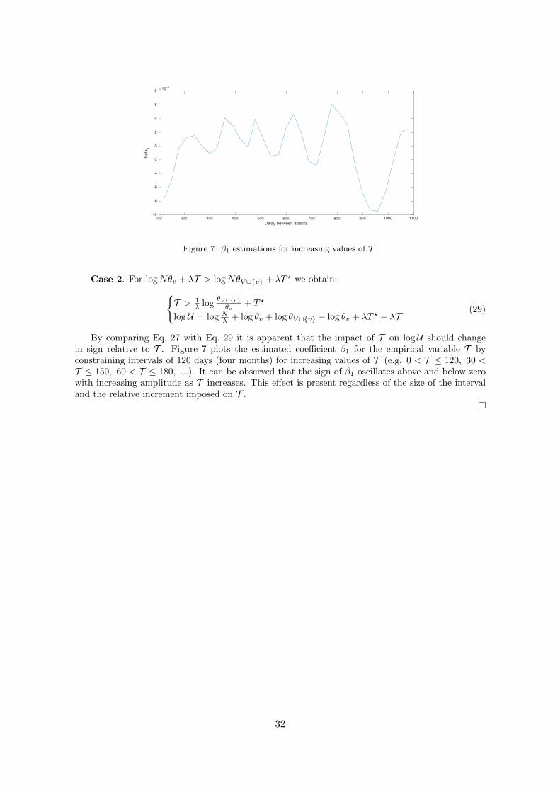
100 200 300 400 500 600 700 800 900 1000 1100
Delay between attacks
-10
-8
-6
-4
-2
0
2
4
6
8
Beta
1
×10-4
Figure 7: β1 estimations for increasing values of T .
Case 2. For logNθv + λT > logNθV ∪{v} + λT ? we obtain:{T > 1
λ logθV∪{v}θv
+ T ?
logU = log Nλ + log θv + log θV ∪{v} − log θv + λT ? − λT
(29)
By comparing Eq. 27 with Eq. 29 it is apparent that the impact of T on logU should changein sign relative to T . Figure 7 plots the estimated coefficient β1 for the empirical variable T byconstraining intervals of 120 days (four months) for increasing values of T (e.g. 0 < T ≤ 120, 30 <T ≤ 150, 60 < T ≤ 180, ...). It can be observed that the sign of β1 oscillates above and below zerowith increasing amplitude as T increases. This effect is present regardless of the size of the intervaland the relative increment imposed on T .
32
7. On-line Appendix: Replication Guide
Here we report the replication guidelines for our study and detail the construction of the tablesfrom WINE, our data can be reproduced by utilizing the reference data set WINE-2012-008, archivedin the WINE infrastructure.
Basic Tables from WINE
The first table we construct from WINE, LIFE, reports the full history of attacks against distinctusers in WINE. It has the following structure:
LIFE =UserID AttackSignature Date SystemID IP HASH VolumeAttacks
......
......
......
where UserID is the unique identifier of a user in the WINE platform, and AttackSignature
is the unique ID identifying the signature that the attempted attack triggered. Date, SystemID,
IP HASH report respectively the day, month and year of the attack; the internal ID of the operatingsystem build; the hash of the IP address. Finally, VolumeAttacks reports how many attacks UserIDreceived on that day.
The attack profile defined in the LIFE table may depend on the interaction between several factors.In particular, we identify three main factors that may confound our observations: the platform
on which the attacked user operates; his/her geographical location; the user evolution. To control forthese factors, we extract two additional tables:
PLATFORM =UserID SystemID OperatingSystem Version ServicePack
......
......
...
PLATFORM links a UserID to the type of system installed on the machine. All systems consideredin this study are running on Microsoft Windows.
TARGET PROFILE =UserID VolumeAttacks Day Month Year
......
......
...
In the TARGET PROFILE table we record the volume of attacks that a UserID receives in a day,irrespectively than the used platform or IP address.
STABILITY =UserID UserID Country SystemID
......
......
In the STABILITY table we record the different countries from which a specific SystemID connected.This can also be obtained by aggregating the data in the table LIFE.
USERS =UserID User Profile Frequency Peak
......
......
33

Finally, we aggregate the data in these two tables in a third extracted table USERS, in which wecategorise each user in WINE over three dimensions: User Profile, Frequency, and Peak. The firstdimension records whether the user changes country and/or updates his or her system within thelifetime of WINE. In Frequency and Peak we record respectively the frequency of received attacksand the maximum volume of attacks received in a day by the user. Aggregated forms of USERS,
PLATFORMS, TARGET PROFILE and STABILITY are disclosed.
Data merging and aggregation
Our final dataset is obtained by first joining the LIFE table with the control tables PLATFORM,
USERS, TARGET PROFILE, and then by performing a self-join of the obtained table with itself. Thegoal of the self-join is to obtain the pairs of subsequent attack signatures triggered by a single user,and the time passed in between the two attacks. The final disclosed table is of the form:
SIGNATURES =
SID 1 SID 2 T U N Country OS OS V OS SP User Profile Frequency Peak...
......
......
......
......
......
...
where SID 1=SignatureID and SID 2=SignatureID later identify respectively the attack signa-ture triggered in the first and the second attack received by the user. T reports the days passedin between the two attacks. U=count(machineID) reports the number of machines affected bySignatureID later T days after receiving an attack of type SignatureID. Similarly,N=sum(volumes
of SignatureID later) counts how many times these two attacks triggered an alarm T days apart.The difference with the previous field is that single machines may receive more than one attack ofthis type, thus we have sum(volumes of SignatureID later) ≥count(machineID). The remainingfields are obtained with a join with the tables PLATFORM, USERS, TARGET PROFILE.
Merging WINE with CVEs
SignatureID and SignatureID later are internal codes that identify which attack signature de-ployed by Symantec’s product the attack triggered. To identify which vulnerability (if any) the attackattempted to exploit we map WINE’s SignatureID with the threat description publicly available atSymantec’s Security Response dataset.12 In the attack description it is provided, when relevant, thevulnerability that the attack exploits, as referenced by the unique CVE vulnerability identifier.13 TheCVE-ID is a standard reference identifier for software vulnerabilities introduced by the MITRE orga-nization and used by all major vulnerability databases such as the National Vulnerability Database,NVD.14
To characterize each vulnerability, we match the CVE-ID reported in the SignatureID with thevulnerability summary reported in the NVD. The information on NVD comprises the name of theaffected software Sw (e.g. Flash in the example above), the latest vulnerable version Ver of thesoftware (in our example Flash 9.0.115 and 9.0.45), and the disclosure date Day.
Further, additional information describing the technical aspects of the vulnerability are also pro-vided. This information can be extracted from the Common Vulnerability Scoring System (CVSS)assessment of the vulnerability. CVSS measures several technical dimensions of a vulnerability toobtain a standardized assessment that can be used to meaningfully compare software vulnerabilities.However, previous studies showed that not all measures show, in practice, enough variability to char-acterize the vulnerabilities Allodi and Massacci (2014). Of the dimensions considered in CVSS, in thisstudy we are specifically interested in the Access Complexity and Imp measures. The former givesan assessment on the ‘difficulty’ associated with engineering a reliable exploit for the vulnerabilityMell et al. (2007). For example, a vulnerability that requires the attacker to win a race condition
12The reference dataset can be found at https://www.symantec.com/security_response/, last accessedJanuary 15, 2017.
13The classifiers are available at http://cve.mitre.org, last accessed January 15, 2017.14Full database can be found at http://nvd.nist.gov, last accessed January 15, 2017.
34

on the affected system in order to successfully exploit kit may be deemed as a High complexity vul-nerability (because the attacker can not directly control the race condition, thus exploitation can beonly stochastically successful). Similarly, Imp gives an assessment on the Confidentiality, Integrityand Availability losses that may follow the exploitation of the vulnerability.
35