the xmm-newton serendipitous survey · the xmm-newton serendipitous survey,, iii. the axis x-ray...
TRANSCRIPT

A&A 469, 27–46 (2007)DOI: 10.1051/0004-6361:20066271c© ESO 2007
Astronomy&
Astrophysics
The XMM-Newton serendipitous survey,,
III. The AXIS X-ray source counts and angular clustering
F. J. Carrera1, J. Ebrero1, S. Mateos1,3, M. T. Ceballos1, A. Corral1, X. Barcons1, M. J. Page2, S. R. Rosen2,3,M. G. Watson3, J. A. Tedds3, R. Della Ceca4, T. Maccacaro4, H. Brunner5, M. Freyberg5, G. Lamer6,
F. E. Bauer7, and Y. Ueda8
1 Instituto de Física de Cantabria (CSIC-UC), Avenida de los Castros, 39005 Santander, Spaine-mail: [email protected]
2 Mullard Space Science Laboratory, University College London, Holmbury St. Mary, Dorking, Surrey, RH5 6NT, UK3 Department of Physics and Astronomy, University of Leicester, Leicester, LE1 7RH, UK4 Osservatorio Astronomico di Brera, via Brera 28, 20121 Milano, Italy5 Max-Planck-Institut für extraterrestrische Physik, Postfach 1312, 85741 Garching, Germany6 Astrophysikalisches Institut Potsdam, An der Sternwarte 16, 14482 Potsdam, Germany7 Columbia Astrophysics Laboratory, Columbia University, Pupin Laboratories, 550 West 120th Street, Room 1418, New York,
NY 10027, USA8 Department of Astronomy, Kyoto University, Kyoto 606-8502, Japan
Received 18 August 2006 / Accepted 9 March 2007
ABSTRACT
Context. Recent results have revised upwards the total X-ray background (XRB) intensity below ∼10 keV, therefore an accurate de-termination of the source counts is needed. There are also contradictory results on the clustering of X-ray selected sources.Aims. We have studied the X-ray source counts in four energy bands: soft (0.5–2 keV), hard (2–10 keV), XID (0.5–4.5 keV) andultra-hard (4.5–7.5 keV) in order to evaluate the contribution of sources at different fluxes to the X-ray background. We have alsostudied the angular clustering of X-ray sources in those bands.Methods. AXIS (An XMM-Newton International Survey) is a survey of 36 high Galactic latitude XMM-Newton observations cov-ering 4.8 deg2 in the Northern sky and containing 1433 serendipitous X-ray sources detected with 5-σ significance. This survey hassimilar depth to the XMM-Newton catalogues and therefore serves as a pathfinder to explore their possibilities. We have combinedthis survey with shallower and deeper surveys, and fitted the source counts with a Maximum Likelihood technique. Using only AXISsources we have studied the angular correlation using a novel robust technique.Results. Our source counts results are compatible with most previous samples in the soft, XID, ultra-hard and hard bands. We haveimproved on previous results in the hard band. The fractions of the XRB resolved in the surveys used in this work are 87%, 85%, 60%and 25% in the soft, hard, XID and ultra-hard bands, respectively. Extrapolation of our source counts to zero flux is not sufficient tosaturate the XRB intensity. Only galaxies and/or absorbed AGN could contribute the remaining unresolved XRB intensity. Our resultsare compatible, within the errors, with recent revisions of the XRB intensity in the soft and hard bands. The maximum fractionalcontribution to the XRB comes from fluxes within about a decade of the break in the source counts (∼10−14 cgs), reaching ∼50%of the total in the soft and hard bands. Angular clustering (widely distributed over the sky and not confined to a few deep fields) isdetected at 99–99.9% significance in the soft and XID bands, with no detection in the hard and ultra-hard band (probably due to thesmaller number of sources). We cannot confirm the detection of significantly stronger clustering in the hard-spectrum hard sources.Conclusions. Medium depth surveys such as AXIS are essential to determine the evolution of the X-ray emission in the Universebelow 10 keV.
Key words. surveys – X-rays: general – cosmology: large-scale structure of Universe
1. Introduction
The X-ray background (Giacconi et al. 1962) records the historyof accretion power in the Universe (Fabian & Iwasawa 1999;Sołtan 1982), and as such its sources and their evolution have
Table 1 and Appendices are only available in electronic form athttp://www.aanda.org Based on observations obtained with XMM-newton, an ESA sci-ence mission with instruments and contributions funded by ESAMember States and the USA (NASA). Tables 2 and 3 are only available in electronic form at the CDSvia anonymous ftp to cdsarc.u-strasbg.fr (130.79.128.5) or viahttp://cdsweb.u-strasbg.fr/cgi-bin/qcat?J/A+A/469/27
attracted considerable attention (Fabian & Barcons 1992). Deeppencil-beam surveys (Loaring et al. 2005; Bauer et al. 2004;Cowie et al. 2002; Giacconi et al. 2002; Hasinger et al. 2001)have resolved most (>90%) of the soft (0.5–2 keV) XRB into in-dividual sources. Most of these turn out to be unobscured andobscured Active Galactic Nuclei (AGN), while at the fainterfluxes a population of “normal” galaxies starts to contribute sig-nificantly to the source counts (Hornschemeier et al. 2003). Athigher energies the resolved fraction is smaller (Worsley et al.2004): 50% between 4.5 and 7.5 keV, and less than 50% between7.5 keV and 10 keV. Models for the XRB based on the UnifiedModel for AGN successfully reproduce its spectrum with a com-bination of unobscured and obscured AGN, the latter being the
Article published by EDP Sciences and available at http://www.aanda.org or http://dx.doi.org/10.1051/0004-6361:20066271Article published by EDP Sciences and available at http://www.aanda.org or http://dx.doi.org/10.1051/0004-6361:20066271

28 F. J. Carrera et al.: The XMM serendipitous survey. III.
dominant population (Setti & Woltjer 1989; Gilli et al. 2001).Recent hard X-ray AGN luminosity function results (Ueda et al.2003; La Franca et al. 2005) show that such simple models needconsiderable revision, with a lower absorbed AGN fraction athigher luminosities and luminosity dependent density evolutionof the hard X-ray AGN luminosity.
The fainter sources from deep surveys do not contributemuch to the final XRB intensity and are often too faint opticallyand in X-rays to be studied individually. Stacking X-ray spec-tra is a valuable technique in these circumstances (Worsley et al.2006; Civano et al. 2005), but only average properties can be de-duced and this method does not account for the diversity in thenature of the sources necessary to account for the XRB. Wideshallow surveys over a large portion of the sky (Schwope et al.2000; Della Ceca et al. 2004; Ueda et al. 2003) detect minoritypopulations and allow studies of sources on an individual basiswhile serving as a framework against which to study and detectevolution, but again with only a minor contribution to the XRB.
Medium depth wide-band surveys combining many sourceswith relatively wide sky coverage (Hasinger et al. 2007; Pierreet al. 2004; Barcons et al. 2002; Baldi et al. 2002) have the po-tential to provide many of the missing pieces of the XRB/AGNpuzzle, since most (30–50%) of the XRB below 10 keV comesfrom sources at intermediate fluxes (Fabian & Barcons 1992;Barcons et al. 2006), and the optical and X-ray spectra of manysources can be studied individually (e.g. Mateos et al. 2005).Furthermore, extensive XMM-Newton source catalogues areavailable (1XMM1 -SSC 2003-), and significantly larger oneswill become available in the near future (2XMM,. . .), which,since they are constructed from serendipitous sources in typi-cal public XMM-Newton observations, are themselves mediumflux surveys. The exploitation of the full potential of these cata-logues depends on the results from “conventional” smaller scale,medium flux surveys such as those above and the one presentedhere.
Since AGN are the dominant population at medium and lowX-ray fluxes, and X-ray selected AGN are known to clusterstrongly (Yang et al. 2006; Gilli et al. 2005; Mullis et al. 2004;Carrera et al. 1998), it is interesting to investigate the angularclustering of X-ray sources, which can be performed without re-sorting to expensive ground-based spectroscopy. Angular corre-lation can be translated into spatial clustering via Limber’s equa-tion (Peebles 1980), if the luminosity function of the populationsinvolved is known from other surveys. Several studies have in-vestigated the angular clustering in the soft and hard bands onscales ranging from tens or hundreds of arcsec to degrees, withvarying success in the detection of signal. Angular clusteringhas been detected in the soft band (Gandhi et al. 2006; Basilakoset al. 2005; Akylas et al. 2000; Vikhlinin & Forman 1995) withdifferent values of the clustering strength. Angular clustering inthe hard band has evaded detection in some cases (Gandhi et al.2006; Puccetti et al. 2006), but not in others (Yang et al. 2003;Basilakos et al. 2004) where clustering strengths are found tobe marginally compatible with the observed spatial clustering ofoptical and X-ray AGN.
We present here a medium X-ray survey which includes1433 serendipitous sources over 4.8 deg2 of the northernsky: AXIS (An X-ray International Survey). This survey was
1 The first XMM-Newton Serendipitous Source Catalogue (1XMM),released in 2003, contains source detections drawn from 585 XMM-Newton EPIC observations and a total of ∼30 000 individual X-raysources. The median 0.2–12 keV flux of the catalogue sources is∼3 × 10⁻¹⁴ cgs, with ∼12% of them having fluxes below 10−14 cgs.
undertaken under the auspices of the XMM-Newton SurveyScience Centre2 (SSC). In this paper we present the source cata-logue (Sect. 2), overall X-ray spectral properties (Sect. 3), num-ber counts (Sect. 4, where some other samples have also beenused), fractional contribution to the XRB (Sect. 5) and angularclustering properties (Sect. 6). Overall results are summarisedin Sect. 7. In a forthcoming paper (Barcons et al. 2007) wepresent the optical identifications of a subsample of AXIS, whichwe have called the XMM-Newton Medium Survey (XMS). Acomplementary medium sensitivity study of optically identifiedsources in the southern hemisphere is also in preparation (Teddset al. 2007). In this paper we will use cgs as a shorthand for thecgs system units for the flux: erg cm−2 s−1.
2. The X-ray data
2.1. Selection of fields
A total of 36 XMM-Newton observations were selected for op-tical follow-up of X-ray sources within the AXIS programme(see Table 1), with a preference for those that were public earlyin the mission (mid 2000), or part of the SSC Guaranteed TimeProgram. We selected fields having |b|> 20, total exposure time>15 ks, and excluding (optical and X-ray) bright or extendedtargets (except in two cases: A1837 and A399). After discardingthe observing intervals within observations having high back-ground rates, a few of the fields have final exposure times shorterthan 15 ks. A few fields (some with shorter exposure times) werealso included to expand the solid angle for bright X-ray sources.All of these fields have been used for the study of cosmic vari-ance, the angular correlation function and the determination oflog N − log S in different bands.
27 of the original 36 XMM-Newton observations were se-lected for optical follow-up of medium flux X-ray sources. Twoof those 27 fields (A2690 and MS2137) were later excluded fromthe main identification effort because their Declination was toolow to observe them from Calar Alto (Spain) with airmass lowerthan 2. The sources in the remaining 25 fields were used to formflux-limited samples in the 0.5–2 keV, 2–10 keV, 0.5–4.5 keVbands and a non-flux-limited sample in the 4.5–7.5 keV bandand these constitute the final XMS sample (see Barcons et al.2007). These 25 fields are marked in Table 1.
2.2. Data processing and relation to 1XMM
The data used in our earlier follow-up efforts (see previousSection) were originally processed with very different versionsof the SAS ( Science Analysis System, Gabriel et al. 2004). Thereprocessing for the 1XMM catalogue (SSC 2003) provided amuch more homogeneous set of X-ray data. The ObservationData Files (ODF) were processed in the SSC Pipeline ProcessingSystem (PPS) facilities at Leicester with the same SAS versionused for 1XMM (very similar to SAS version 5.3.3, see belowfor the difference), except for the field Mkn 205, which was pro-cessed with SAS version 5.3.3. PHL1092 is a special case sincethe original XMM-Newton observation was never reprocessedand instead we used a newer set of data from the XMM-NewtonScience Archive, which was processed later with a different SASversion (5.4.0).
2 The XMM-Newton Survey Science Centre is an international col-laboration involving a consortium of 10 institutions appointed by ESAto help develop the software analysis system, to pipeline process allthe XMM-Newton data, and to exploit the XMM-Newton serendipitoussource detections, see http://xmmssc-www.star.le.ac.uk
F. J. Carrera et al.: The XMM serendipitous survey. III. 29
The main difference between the versions of the SAS sourcedetection task (emldetect) used for Mkn205 and the rest of thefields is the inclusion of the possibility of sources with negativecount rates in the latter. Negative count rates in individual en-ergy bands were allowed to avoid a bias in the total count ratesof sources that were undetected in one or more energy bands.However, since this option caused numerical problems in somecases, the count rates were limited to values ≥0 in later versionsof the pipeline. Since negative count rates are meaningless, wehave set all the negative count rates to zero in what follows. Thecorresponding detection likelihoods have also been set to zero,ensuring that the presence of that source in that band does notimprove the fit (see below for details).
The standard SAS products include X-ray source lists (cre-ated by emldetect) for each of the three EPIC cameras (MOS1,MOS2, Turner et al. 2001, and pn, Strüder et al. 2001), deter-mined in five independent bands (1: 0.2–0.5 keV, 2: 0.5–2.0 keV,3: 2.0–4.5 keV, 4: 4.5–7.5 keV, and 5: 7.5–12.0 keV). In addi-tion, the source detection algorithm was run in the 0.5–4.5 keV(band 9), which we will call the XID band. Since EPIC pn hasthe highest sensitivity of the three cameras, we have used onlypn source lists. We have not allowed for source extent when de-tecting the sources, and therefore all the sources in our surveyare treated as point like.
The internal calibration of the source positions from the SASis quite good (1.5 arcsec, Ehle et al. 2005), but there may besome systematic differences between the absolute X-ray sourcepositions and optical reference frames. We have registered theX-ray source positions to the USNO-A2 reference frame field byfield, using the SAS task eposcorr. This task shifts the X-rayreference frame to minimise the differences between the X-raysource positions and the positions of their optical counterparts ina given reference astrometric catalogue (USNO-A2 in our case).These corrected positions are given in Table 2. The average shiftin absolute value in RA (Dec) was 1.3 (0.9) arcsec, and in allcases the shifts were under 3 arcsec. The average number ofX-ray-USNO-A2 matches used to calculate the shifts was 28(the minimum was 16 and the maximum 82). There were twofields for which this procedure failed (Mkn3 and A399), prob-ably in the first case because one quarter of the pn chips werein counting mode, and in the second case two moderately strongextended sources are located in opposite corners of the field. Wetherefore used the original X-ray source positions for these twofields.
2.3. Source selection
In each detection band the source detection algorithm fits a por-tion of the image around the position of the candidate source,trying to match the Point Spread Function (PSF) shape to thephoton distribution. In this process it uses the background mapand the exposure map to fit a source count rate and 2D position.The typical size of this region is the 80% encircled energy ra-dius, which corresponds to about 5 pixels on-axis and 7 pixelsat 15 arcmin off-axis (we have used 4 arcsec pixels throughout).Sources closer than this distance away from the pn chip edgesmay have a worse determination of their positions and/or countrates. We have therefore excluded all sources closer than the 80%encircled energy radius (taking into account the off-axis angle)to any pn chip edges. A region (∼12 pixels wide) on the readout(outer) edge of the pn chips is masked out on board the satellite(Ehle et al. 2005). We have considered this “effective” edge asthe outer edge of each chip when defining our excluded regions.
We have visually inspected all X-ray images, excluding cir-cular regions around bright targets, and other bright/extendedsources in the images (see Table 1 for the sizes and positionsof these regions). In a few images a bright band extending fromthe target to the pn chip reading edge was visible, due to the pho-tons arriving at the detector while it was being read out (calledthe Out Of Time – OOT – region). We have excluded a rectangu-lar region around the OOT region, whose width is also given inTable 1. In addition, sources affected by bright pixels/segmentshave been excluded as well as those which were obviously af-fected by the presence of nearby bright sources, or split by thechip gaps and not picked up by the above procedures.
In addition there were two sets of fields which partially over-lapped: G133-69pos_2 and G133-69Pos_1 on the one hand andSDS-1b, SDS-2 and SDS-3 on the other. We have dealt with thisby masking out the portion of the second (and third) field whichoverlap with the first field, in the order given above.
We have used the following bands in the analysis performedin this paper:
– soft: 0.5–2 keV, identical to the standard SAS band 2;– hard: combining standard SAS bands 3, 4 and 5 and hence
corresponding to counts in the 2 to ∼12 keV range. However,we have calculated (and will quote) all hard fluxes in2–10 keV;
– XID: 0.5–4.5 keV, identical to the SAS band 9;– ultra-hard: 4.5–7.5 keV, identical to the standard SAS band 4.
The detection likelihood in the hard band (L345) was obtainedfrom the detection likelihoods in bands 3, 4 and 5 (L3, L4, andL5 respectively) using L345 = − log(1 − Q(5/2, L′3 + L′4 + L′5)),where L′i can be obtained from Li = − log(1 − Q(3/2, L′i)) andQ(a, x) is the incomplete gamma function (see emldetectdocumentation).
There were a total of 2560 accepted sources with anemldetect detection likelihood ≥10 (the default value) in atleast one band. These are listed in Table 2 with their correctedX-ray positions and count rates in the standard SAS and XIDbands.
The original unfiltered source lists are identical to the onesused by Mateos et al. (2005) in their study of the detailed spec-tral properties of medium flux X-ray sources for the fields com-mon to both studies. They also used similar criteria for exclud-ing sources close to the pn chip edges except in the case of thereadout edge. The differences in the final accepted source listsarose for several reasons: Mateos et al. used sources close to pnchip gaps (which we have excluded) if they were far from chipgaps in the MOS detectors. They excluded from their spectralanalysis the sources with a low number of counts. Finally, wehave treated the sources close to the exclusion zone boundariesslightly differently. These differences are at the 10% level: out ofthe final 1137 accepted sources in the Mateos et al. sample, only119 would have been excluded by our criteria.
2.4. Sensitivity maps
The value of the sensitivity map at a given point is the minimumcount rate for a source to be detected with the desired likelihoodat that point. As explained above, the detection likelihood as-signed by emldetect takes into account the number of countsin the detection box, how well they fit the PSF shape and thevariation of the exposure map over the detection box. The likeli-hood is therefore, in principle, not trivially related to the Poissonprobability of an excess in the number of detected counts overthe expected background in the detection box.
30 F. J. Carrera et al.: The XMM serendipitous survey. III.
However, we have found (see Appendix A) that the countrate assigned by the software to the source (the “observed” countrate) is proportional to the count rate expected from a Poissondistribution for the same likelihood (for detection likelihoods be-tween 8 and 20), with proportionality constant∼0.9−1.1 depend-ing on the band. It appears that the non-Poisson characteristicstaken into account by emldetect have a relatively small influ-ence on the determination of the count rate. For a given like-lihood, radius of the detection region, total value of the back-ground map and average value of the exposure map in that re-gion we calculated the expected Poisson count rate at each pointof the detector using the proportionality constants for the corre-sponding “observed” count rate, i.e. the value of the sensitivitymap (see Appendix A for further details).
We have used the above procedure to create sensitivity mapsfor each field in each band in image (X, Y) coordinates, whichhave 4 arcsec pixels with sky North towards the top and East tothe left and are centred approximately in the optical axis of theX-ray telescope. We have also taken into account for each fieldthe areas excluded close to the detector edges, and around thebright sources and OOT regions, excluding those regions fromthe sensitivity maps as well.
The final selection of sources in each band was done usingtheir detection likelihood and the corresponding sensitivity mapat their given sky position (to ensure the validity of the sky ar-eas calculated from the sensitivity maps, see Sect. 4.1). We havechosen a detection confidence limit of 5-σ which correspondsto L = 15 in the band under consideration. We have also im-posed that the source has a count rate equal to or larger than thevalue of the sensitivity map at that sky position, to ensure thatthe source detection is reliable. This excluded less than 5% ofthe L ≥ 15 sources in the soft band, ∼10% of the sources in theXID and ultra-hard bands and ∼20% of the sources in the hardband. The number of sources excluded by this criterion is muchlarger in the hard band than in the other bands. This somewhatcontradicts the proportionality between the detected count rateand the Poisson count rate for this band being in a different di-rection than in the other bands (∼10% smaller rather than ∼10%larger, see Table A.1), since the sensitivity map will then be rel-atively lower and therefore would tend to include more sourcesrather than exclude them. In any case, the hard band is the widestand the only one of our bands which is not one of the bands usedfor source searching in the SAS, being instead a composite ofthree default bands. In principle, all this makes the hard bandthe more complex to deal with and for which therefore the un-certainties associated with our empirical method to calculate thesensitivity maps might be highest.
The total number of distinct selected sources, that is fulfillingthe above criteria in at least one of the bands, is 1433. We givein Table 4 the total number of selected sources in each of theabove bands. Unless explicitly stated otherwise, for the log N −log S and the angular clustering analyses below we have onlyused sources detected in the corresponding bands. However, itis important to emphasise that if a source has been detected inat least one band it can be considered to be a real source andtherefore its counts in other bands can be used, e.g. for spectralfitting or hardness ratio calculations, even if the source has acount rate smaller than the detection threshold in those bands.
To estimate the number of spurious sources in our surveywe first need to calculate the number of independent source de-tection cells. emldetect uses an input list from eboxdetect,which is a simple sliding-box algorithm using a square 5×5 pixels detection cell. Therefore the individual detection cellis 5 × 5 × (4′′)2 = 400 arcsec2. The total area of our survey is
∼4.8 deg2 (see Sect. 4.1) or about 155 520 independent detectioncells. Since the probability of a false detection at the 5-σ level is0.000057, this corresponds to about 9 spurious sources in eachof our detection bands. This is less than 1% in the soft and XIDbands, about 2% in the hard band and almost 10% in the ultra-hard band. The latter fraction could partly explain the discrepantpoint in the ultra-hard log N − log S at the lowest fluxes (seeSect. 4.5), since it is there where the contribution from spurioussources is expected to be highest.
3. X-ray properties of the sources
We have studied the broad spectral characteristics of our sourcesby fitting their count rates in several bands to those expectedfrom power-law spectra with photon index Γ and GalacticHydrogen column densities (NH) from 21 cm radio measure-ments (Dickey & Lockman 1990, see Table 1). The spectra of afew sources will obviously not be well represented by a power-law (e.g. stars or clusters showing thermal spectra), but for thepurpose of calculating fluxes in bands in which the power-lawwas fit, a power-law is a reasonably accurate and very simpleapproximation.
The expected count rates for different values of Γ (from −10to 10 in steps of 0.5, interpolating linearly for intermediate val-ues) and the Galactic NH values of each field were calculatedwith xspec (Arnaud 1996), using the “canned” on-axis redis-tribution matrix files and on-axis effective areas for each fieldcreated with the SAS task arfgen. The inaccuracies arisingfrom using standard response matrices instead of source spe-cific matrices (as generated by rmfgen) are expected to be smallsince we only use broad bands, much broader than the spectralresolution of the EPIC pn camera. Since the count rates fromemldetect are corrected for the exposure map (which includesvignetting and bad pixel corrections) and the PSF enclosed en-ergy fraction, the effective areas were generated while disablingthe vignetting and PSF corrections, as indicated in the arfgendocumentation.
The corresponding fluxes in bands 2 to 5 (in the case of band5 the flux was calculated in the 7.5 to 10 keV band) were alsocalculated using the spectral model for the same values of Γ,setting NH = 0. We have checked that the relatively coarse sam-pling does not introduce any biases in our spectral fits by re-peating the spectral fits for one field with a step in Γ of 0.001.The results were essentially identical with any differences in thespectral slopes being much smaller than their uncertainties.
We have performed spectral fits in bands 2 and 3 (for the softand XID fluxes) and bands 3, 4 and 5 (for the hard and ultra-hardfluxes). The average count rates of our selected sources in theXID and hard bands are 0.0095 and 0.0032, respectively, whichfor a typical exposure time of 15 ks give an average of more than10 counts per bin. This ensures that Gaussian statistics are a goodapproximation here. However, these count rates are not sufficientin many cases to warrant a detailed spectral fitting with xspec.The best fit Γ and flux were calculated by minimising the χ2 be-tween the observed and expected count rates. The minimisationwas actually done in Γ, setting the flux from the normalisationthat minimised the χ2 in the corresponding band. One sigma er-ror bars for the photon index and flux were obtained from thevalues which produced ∆χ2 = 1 from the minimum. These errorbars were asymmetric in most cases but we have used a sym-metric error bar (the arithmetic average of the upper and lowererror bars) for the weighted averages of the spectral slopes andthe log N − log S . In a few cases the fitted photon indices arevery steep with |Γ | ∼ 10. In all cases this corresponds to sources
F. J. Carrera et al.: The XMM serendipitous survey. III. 31
Table 4. Number of sources selected in different bands N, weightedaverage slopes 〈Γ〉 and errors (taking into account both the error barsin the individual Γ and the dispersion around the mean), and numberof observed sources used in the average Nave. The soft, hard, XID andultra-hard bands are as defined in the text. “Soft and hard” refers tosources selected simultaneously in the soft and hard bands, “Only soft”refers to sources selected in the soft band but not in the hard band, and“Only hard” refers to sources selected in the hard band and not in thesoft band.
0.5–4.5 keV 2–10 keVSelection N Nave 〈Γ〉 Nave 〈Γ〉Soft 1267 1239 1.811 ± 0.015 1145 1.53 ± 0.02Hard 397 397 1.76 ± 0.03 394 1.55 ± 0.03XID 1359 1335 1.773 ± 0.016 1244 1.47 ± 0.02Ultra-hard 91 91 1.80 ± 0.06 91 1.50 ± 0.07Soft and hard 345 345 1.79 ± 0.03 342 1.67 ± 0.03Only soft 922 894 1.878 ± 0.017 803 1.04 ± 0.04Only hard 52 52 −0.29 ± 0.08 52 0.53 ± 0.12
with positive count rates in only one of the fitted bands, forc-ing the power law to the steepest allowed slope. The number ofthese pathological cases in each band can be obtained from thedifference between the N and Nave columns in Table 4 (typically<10%).
The photon indices and fluxes in each of the fitted bands aswell as their error bars are given for each source in Table 3. Weshow in Table 4 the weighted average photon indices of the de-tected sources in each of the fitted bands as well as the numberof sources used in the averages, excluding in all cases sourceswith | Γ |> 9 to avoid biasing the averages with a few outliers.The impact of excluding these sources would be small for theweighted averages used here.
We have checked the reliability of our simple spectral fitmethod (see Appendix B), performing both internal tests withsimulations and external checks with respect to the full spectralfits of Mateos et al. (2005) to a set of sources with a large over-lap. We conclude that our 2–3 band spectral slopes are sufficientwhen taken individually for the purposes of calculating fluxesin different bands. However, we have found that there are sig-nificant systematic biases in the average photon indices, whenaveraged over large samples, which are larger than the statisticalerrors. These systematic biases are nonetheless small in both ab-solute (∆Γ ∼ 0.12) and relative (∆Γ/Γ = 0.2) terms. Our methodis therefore adequate for extracting broad spectral informationfrom medium flux X-ray sources such as those in the 1XMMand 2XMM catalogues.
In broad terms, the soft/XID band slopes are ∼1.8 for sourcesdetected in all bands, being slightly softer for sources detectedonly in the soft band and much harder for sources detected onlyin the hard band (see Table 4). The hard band slopes are flatter,closer to 1.5–1.6, but slightly steeper for sources detected bothin the soft and hard bands (∼1.7). The average hard slope of thesources only detected in the soft band is quite flat 〈Γ〉 ∼ 1, buttheir un-weighted average is 〈Γ〉 = 1.53±0.08, much closer to theother average slopes in that band. The origin of this difference isthat “Only soft” sources with steep spectra in the hard band tendto have larger errors in the hard spectral slope (because they havefew counts in XMM-Newton bands 4 and 5 and so the slopeis not well constrained), and therefore they have a very smallweight in the weighted average.
The difference between the spectral slopes of sources onlydetected in in the soft band and those only detected in the hard
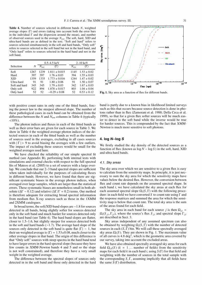
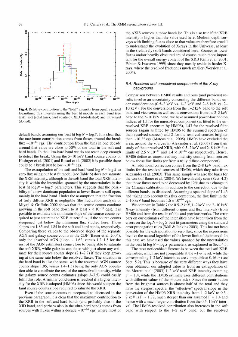
Fig. 1. Sky area as a function of flux for different bands.
band is partly due to a known bias in likelihood limited surveyssuch as this that occurs because source detection is done in pho-tons rather than in flux (Zamorani et al. 1988; Della Ceca et al.1999), so that for a given flux softer sources will be much eas-ier to detect in the soft band while the inverse would be truefor harder sources. This is compounded by the fact that XMM-Newton is much more sensitive to soft photons.
4. log N−log S
We firstly studied the sky density of the detected sources as afunction of flux (known as log N − log S ) in the soft, hard, XIDand ultra-hard bands.
4.1. Sky areas
The sky area over which we are sensitive to a given flux is easyto calculate from the sensitivity maps. In principle, it is just nec-essary to sum the sky area for which the sensitivity maps havevalues below the desired flux. However, the conversion betweenflux and count rate depends on the assumed spectral shape. Ineach band i, we have calculated the sky areas at each flux foreach assumed spectral slope Ωi(S , Γ) with the following proce-dure: in each field we have converted S to count rate using Γ andthe response matrices and summed the area for which the sensi-tivity map is below that count rate. The total sky area is the sumof the areas found for each field.
The sky area in each band for each source j is then Ω j,i =Ωi(S j,i, Γ j,i), where the source’s flux S j,i and spectral slope Γ j,i
are described in Sect. 3.Sky areas independent of any assumed spectrum can also
be obtained by weighting Ωi(S , Γ) with the number of detectedsources in each (S , Γ) bin. We will call these spectrally averagedsky areas Ωi(S ). They are shown in Fig. 1. The maximum valueof all curves is 4.8 deg2, which is the geometric area covered byour survey, taking into account the excluded areas.
We have also obtained spectrally averaged sky areas for eachfield Ωi,k(S ) (k = 1 . . . number of fields) from the sensitivitymaps for each field k in each band i, using S (Γ) for that field andweighting with the number of sources in the total sample withthe corresponding S , Γ, assuming implicitly that all fields havethe same S (Γ) distribution.
32 F. J. Carrera et al.: The XMM serendipitous survey. III.
4.2. Data from other surveys
Our survey consists of XMM-Newton exposures with a typicalexposure time of about 15 ks and it is hence a medium survey.Shallower, wider area surveys are required to obtain significantnumbers of bright sources while deeper pencil-beam surveyswill probe fainter fluxes. We have combined our survey withboth shallower and deeper surveys to obtain a wide coveragein flux (∼2–4 orders of magnitude):
– BSS: Della Ceca et al. (2004) have constructed a bright sam-ple of XMM-Newton sources down to a flux of 7×10⁻¹⁴ cgsin the XID band, with a uniform coverage of 28.1 deg2 abovethat flux. This sample ideally complements our survey, beingboth wider and shallower and selected exactly in the sameband with the same telescope (but with a different detector:MOS2 instead of pn). We have used a total of 389 sourcesfrom that survey, including all sources identified as starswhich have been excluded from the log N − log S analysisof Della Ceca et al. (2004)
– HBS: in the same paper, Della Ceca et al. (2004) also de-fine a sample of sources detected in the ultra-hard band,down to the same flux limit and with a uniform coverageof 25.17 deg2, again both shallower and wider than ours andwith the same telescope. Results from a subsample are pre-sented by Caccianiga et al. (2004). The source counts arealso discussed by Della Ceca et al. (2004) and compared toprevious results from BeppoSAX. We have used a total of65 sources from this survey
– CDF: the deepest survey in the soft and hard bands so far isthe Chandra Deep Field North (CDF-N), Bauer et al. (2004),obtained from a total exposure of 2 Ms in a Northern hemi-sphere location. In a complementary effort in the South, theChandra Deep Field South (Giacconi et al. 2001; Rosatiet al. 2002) obtained a total exposure time of 1 Ms. Sourcecounts from both samples have been discussed in Bauer et al.(2004). There are a total of 442 soft and 313 hard sources inthe CDF-N, and 282 soft and 186 hard sources in the CDF-S.Recent internal Chandra calibrations have increased the es-timate of the ACIS effective area above 2 keV. We have usedprocedures available in the Chandra calibration database tocompare data from Cycles 8 and 5: above 2 keV the ra-tio between the effective areas is reasonably flat and wellapproximated by a constant increase factor of about 12%.The increase in the 2–8 keV fluxes is unlikely to be due tothe increasing contamination from the optical blocking filter,since the latter only manifests itself below 1 keV. Therefore,all CDF-N and CDF-S hard fluxes (and their correspond-ing errors) have been decreased by this factor. Furthermore,when comparing the sky areas calculated individually foreach source with those calculated interpolating from the skyarea of the full survey, the faintest soft sources in both CDFsurveys showed large (up to several orders of magnitude) dis-crepancies. Since our maximum likelihood log N − log S fitmethod requires the use of a model for the sky area of the fullsurvey (see Sect. 4.5), we have not used soft sources fainterthan 3 and 7 × 10⁻¹⁷ cgs in the CDF-N and CDF-S respec-tively for fits to log N − log S .
– AMSS: The ASCA Medium Sensitivity Survey (Ueda et al.2005) is one of the largest high Galactic latitude, broad-bandX-ray surveys to date and includes 606 sources over 278 deg2
with hard band fluxes between ∼10−13 and ∼10−11 cgs.
The average sky area as a function of flux for different bandsfor the CDF and AMSS are shown in Bauer et al. (2004) and
Ueda et al. (2005), respectively, and we have used these values(as supplied by the authors) for the Maximum Likelihood fit (seeSect. 4.5). The Chandra re-calibration has also been applied tothe CDF effective area fluxes.
4.3. Construction of the binned log N − log S
The binned differential log N− log S (number of sources per unitflux and unit sky area at a given flux S : dN/dS dΩ) have beenconstructed by summing the inverse of the Ω j,i for the sources ineach flux bin and dividing that number by the width of the bin.The errors are calculated by dividing the dN/dS dΩ by the squareroot of the sources in each bin. Since we have chosen to have aminimum number of sources per bin (see below), their widthsare all in principle different and are determined by the flux ofthe first source in the bin and the flux of the first source in thenext bin as flux increases. By this definition, the width of the lastbin is left undefined. Since we have a large number of sourceswe have dropped the brightest source in each sample (only whendealing with binned log N − log S ) and defined the upper limit inthe last bin to be the flux of this brightest source.
The integral log N − log S relation (number of sources perunit sky area with fluxes higher than S : N(>S )) from our sampleand other samples are shown in Fig. 2. We have chosen to plotthe integral log N − log S relation in bins containing 15 sourceseach (except the last one, which can contain up to 29 sources),to avoid apparent features due to fluctuations of a few sources,especially at the brighter ends of each sample where the numberof sources is low. We have simply added the inverse of the skyareas for each source, Ω j,i, for all sources with fluxes above thelower limit of each bin. The error bars are calculated by dividingthe N(>S ) by the square root of the total number of sources withflux equal or greater than the lower limit of the bin.
Sources just below the faint flux limit of a survey may besubject to statistical fluctuations in their fluxes that promotethem into the survey. Similarly, the fainter sources just abovethat limit could drop out of the survey for the same reason.However, since fainter sources are much more abundant (be-cause the source counts are steep), the net effect is to artifi-cially increase the observed source counts close to the faintersurvey limits. This is known as the Eddington bias (Eddington1913) and may lead to a re-steepening of log N − log S at thefaintest fluxes, as observed in the AXIS ultra-hard source countsfor example.
4.4. log N − log S model
Previous X-ray source count results (e.g. Bauer et al. 2004; Uedaet al. 2003; Moretti et al. 2003; Baldi et al. 2002; Hasinger et al.1998; Cagnoni et al. 1998) have shown that log N − log S is wellapproximated by a steep power law at bright fluxes and flatteningat lower fluxes. We have hence adopted the following model forthe differential log N − log S :
dNdS dΩ
(S ) =
⎧⎪⎪⎪⎨⎪⎪⎪⎩KS b
(SS b
)−Γd, S ≤ S b
KS b
(SS b
)−Γu, S > S b
⎫⎪⎪⎪⎬⎪⎪⎪⎭ ·
The above model has four independent parameters: the breakflux S b, the normalisation K, the slope at high fluxes Γu and theslope at low fluxes Γd. If the change in the slope of log N − log Sis not significant we fixed S b ≡ 10−14 cgs and Γu = Γd, leavingonly two independent variables: K and Γu.
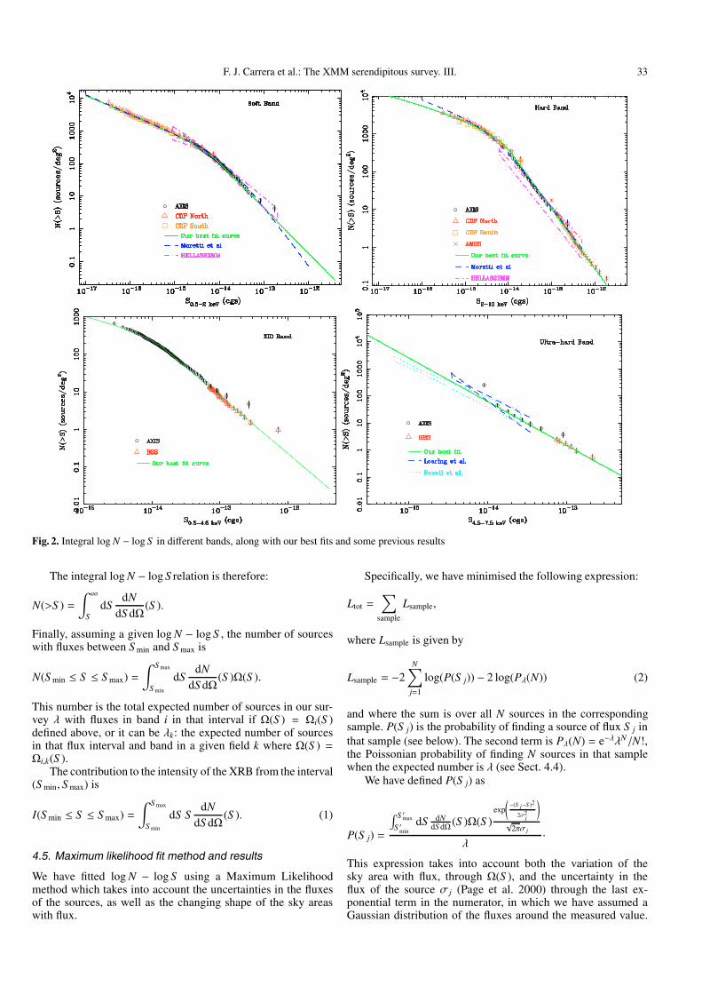
F. J. Carrera et al.: The XMM serendipitous survey. III. 33
Fig. 2. Integral log N − log S in different bands, along with our best fits and some previous results
The integral log N − log S relation is therefore:
N(>S ) =∫ ∞
SdS
dNdS dΩ
(S ).
Finally, assuming a given log N − log S , the number of sourceswith fluxes between S min and S max is
N(S min ≤ S ≤ S max) =∫ S max
S min
dSdN
dS dΩ(S )Ω(S ).
This number is the total expected number of sources in our sur-vey λ with fluxes in band i in that interval if Ω(S ) = Ωi(S )defined above, or it can be λk: the expected number of sourcesin that flux interval and band in a given field k where Ω(S ) =Ωi,k(S ).
The contribution to the intensity of the XRB from the interval(S min, S max) is
I(S min ≤ S ≤ S max) =∫ S max
S min
dS SdN
dS dΩ(S ). (1)
4.5. Maximum likelihood fit method and results
We have fitted log N − log S using a Maximum Likelihoodmethod which takes into account the uncertainties in the fluxesof the sources, as well as the changing shape of the sky areaswith flux.
Specifically, we have minimised the following expression:
Ltot =∑
sample
Lsample,
where Lsample is given by
Lsample = −2N∑
j=1
log(P(S j)) − 2 log(Pλ(N)) (2)
and where the sum is over all N sources in the correspondingsample. P(S j) is the probability of finding a source of flux S j inthat sample (see below). The second term is Pλ(N) = e−λλN/N!,the Poissonian probability of finding N sources in that samplewhen the expected number is λ (see Sect. 4.4).
We have defined P(S j) as
P(S j) =
∫ S ′max
S ′mindS dN
dS dΩ (S )Ω(S )exp
(−(S j−S )2
2σ2j
)√
2πσ j
λ·
This expression takes into account both the variation of thesky area with flux, through Ω(S ), and the uncertainty in theflux of the source σ j (Page et al. 2000) through the last ex-ponential term in the numerator, in which we have assumed aGaussian distribution of the fluxes around the measured value.

34 F. J. Carrera et al.: The XMM serendipitous survey. III.
Table 5. Maximum likelihood fit results to log N − log S in different bands and using different samples: the first column is the band used, thesecond is the power-law slope above the flux break, the third is the slope below that break, the fourth is the flux break, the fifth is the normalisationand the last six columns indicate the number of sources from each sample used in the fit.
Nused/Ntot
Band Γu Γd S b K AXIS BSS HBS CDF-N CDF-S AMSS(10−14 cgs) (deg−2)
softg 2.40+0.06−0.07 1.74+0.06
−0.07 1.15+0.18−0.19 120.0+22
−18 1267/1267soft 2.39+0.06
−0.06 1.69+0.07−0.06 1.15+0.16
−0.13 123.4+18.8−17.1 1267/1267
soft f 2.38+0.14−0.09 1.56+0.01
−0.01 1.02+0.14−0.17 141.4+42.1
−7.3 1267/1267 429/442a 269/282b
hardg 2.74+0.08−0.07 - 1.00 735 +92
−76 348/397c
hard 2.72+0.07−0.08 - 1.00 684.4+74.1
−84.0 348/397c
hard 2.03+0.12−0.11 1.00+0.11
−0.12 0.30+0.07−0.05 1086.6+134.3
−146.5 313/313hard 2.51+0.50
−0.28 0.89+0.12−0.12 0.72+0.11
−0.10 743.7+109.6−105.6 186/186
hard 2.12+0.13−0.01 1.10+0.01
−0.01 0.44+0.04−0.01 799.1+226.8
−8.4 313/313 186/186hard 2.66+0.08
−0.05 1.20+0.01−0.01 1.00+0.08
−0.01 611.5+49.1−34.3 397/397 313/313 186/186
hard 2.58+0.02−0.02 - 1.00 606.5+46.8
−46.3 348/397c 606/606hard 2.53+0.25
−0.18 1.18+0.14−0.08 0.92+0.66
−0.19 607.8+366.4−208.1 313/313 186/186 606/606
hard f 2.58+0.17−0.02 1.30+0.01
−0.01 1.17+0.01−0.05 485.3+10.1
−24.3 397/397 313/313 186/186 606/606
XIDg 2.39+0.05−0.20 1.37+0.09
−0.32 1.08+0.07−0.48 265 +214
−19 1359/1359XID 2.46+0.11
−0.07 1.29+0.09−0.18 1.45+0.16
−0.26 212.2+47.4−22.8 1359/1359
XID f 2.54+0.03−0.04 1.35+0.06
−0.25 1.64+0.13−0.28 193.0+33.1
−15.8 1359/1359 389/389
ultra-hardg 2.63+0.15−0.15 - 1.00 102 +23
−20 84/89d
ultra-hard 2.59+0.09−0.05 - 1.00 95.0+11.1
−12.8 84/89d
ultra-hard f 2.62+0.10−0.10 - 1.00 102.2+20.0
−21.1 84/89d 58/65e
a S min,CDF−N = 3 × 10⁻¹⁷ cgs; b S min,CDF−S = 6 × 10⁻¹⁷ cgs; c S min,AXIS = 1.5 × 10⁻¹⁴ cgs; d S min,AXIS = 10−14 cgs; e S max,HBS = 2.5 × 10⁻¹³ cgs;f Best fit used for contribution to XRB, and in Figs. 2 and 3; g Using fixed photon indices of 1.8 in the soft and XID bands, and 1.7 in the hard andultra-hard bands.
To speed up the numerical calculation of the integral in the nu-merator above we have defined S ′min = max(S j − 4σ j, S min) andS ′max = min(S j+4σ j, S max), since the tails of the Gaussian distri-bution decrease very quickly. The normalisation of log N− log S(K) appears both in the numerator and the denominator of P(S j)and it is unconstrained. This is why we have introduced the sec-ond term in Eq. (2).
The 1-σ uncertainties in the log N − log S parameters are es-timated from the range of each parameter around the minimumwhich makes ∆Ltot = 1. For each parameter this is performedby fixing the parameter of interest to a value close to the best fitvalue and varying the rest of the parameters until a new mini-mum for the likelihood is found. This procedure is repeated forseveral values of the parameter until this new minimum equalsLtot,min + 1.
The results of the Maximum Likelihood fits to various (sin-gle and combined) samples and bands are given in Table 5.Except when stated otherwise the flux interval used in the fitis S min = 10−17 cgs and S max = 10−12 cgs. These numbers havebeen chosen to span the observed fluxes of the sources. The finalresults are not very dependent on them, since the sky area fallsvery quickly at low fluxes and the sky density of bright sourcesis very small. The initial values for the numerical search for thebest fit have been obtained from a χ2 fit to the total binned differ-ential log N − log S . The best overall fits are marked in the firstcolumn of Table 5 and also shown in Fig. 2.
The first two rows in Table 5 for each band allow comparisonof the results of the fit to the AXIS sources, using a fixed spectralslope to calculate fluxes and sky areas (Γ = 1.8 in the soft andXID bands, Γ = 1.7 in the hard and ultra-hard bands, first row),to the results using the best fit spectral slope for each source(second row). The results are mutually compatible in all bands
but the error bars are noticeably larger in the XID and ultra-hard band when using a fixed spectral slope. In fitting the spec-tra of the sources we effectively “force” them to have a powerlaw spectral shape and hence the uncertainties in the fitted fluxesare smaller than those in the fluxes with fixed spectral slopes.This might at least partly explain the smaller uncertainties in thelog N − log S fitted parameters in the latter case. In what followswe have thus used the slopes from spectral fits to calculate fluxesfrom count rates for all the AXIS sources, since this approachseems to produce smaller uncertainties in the fitted parameters.
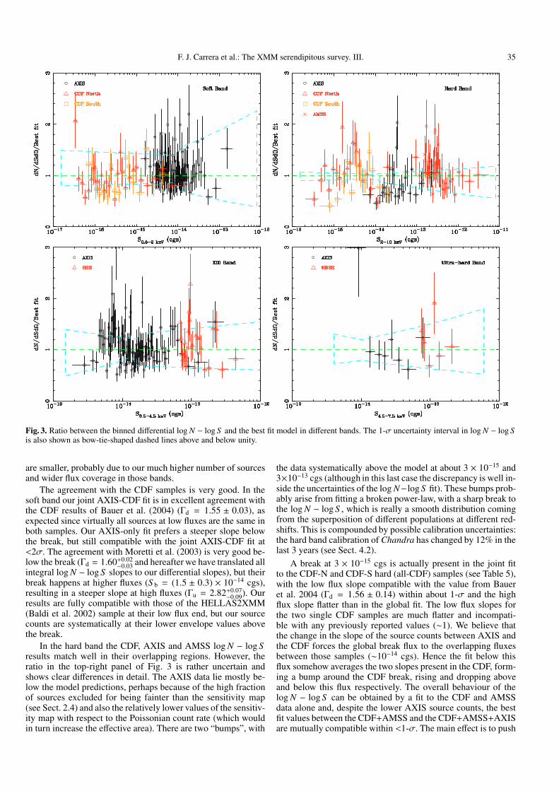
There is general agreement between data and model fits butit is difficult to quantify this statement, since, unlike the χ2 statis-tic, the absolute value of Ltot is not an indicator of the goodnessof fit. Each panel in Fig. 2 covers several orders of magnitudeand hence a detailed visual comparison is also difficult. We havetherefore plotted in Fig. 3 the ratio between the binned differen-tial log N − log S and the best fit model. Systematic deviationsfrom unity in those plots would reveal differences between thedata and the best fit model. In that Figure we also show the 1-σuncertainty interval on the best fit which is estimated in a conser-vative manner: for each flux we have calculated the differentiallog N − log S in the 16 corners of the hypercube defined by the1-σ uncertainty intervals in the best fit log N − log S parametersand taken the maximum and minimum values.
As expected, the relative agreement of the AXIS andBSS/HBS source counts is quite good, merging with each otherwell and following the same log N − log S shape. This confirmsthe good relative calibration of the two EPIC cameras on boardXMM-Newton (pn for AXIS and MOS2 for BSS/HBS). TheXMM-COSMOS log N − log S results (Cappelluti et al. 2007)are also consistent with our results within 1 to 2-σ in the softand hard bands, but the uncertainties in our best fit parameters
F. J. Carrera et al.: The XMM serendipitous survey. III. 35
Fig. 3. Ratio between the binned differential log N − log S and the best fit model in different bands. The 1-σ uncertainty interval in log N − log Sis also shown as bow-tie-shaped dashed lines above and below unity.
are smaller, probably due to our much higher number of sourcesand wider flux coverage in those bands.
The agreement with the CDF samples is very good. In thesoft band our joint AXIS-CDF fit is in excellent agreement withthe CDF results of Bauer et al. (2004) (Γd = 1.55 ± 0.03), asexpected since virtually all sources at low fluxes are the same inboth samples. Our AXIS-only fit prefers a steeper slope belowthe break, but still compatible with the joint AXIS-CDF fit at<2σ. The agreement with Moretti et al. (2003) is very good be-low the break (Γd = 1.60+0.02
−0.03 and hereafter we have translated allintegral log N − log S slopes to our differential slopes), but theirbreak happens at higher fluxes (S b = (1.5 ± 0.3) × 10−14 cgs),resulting in a steeper slope at high fluxes (Γu = 2.82+0.07
−0.09). Ourresults are fully compatible with those of the HELLAS2XMM(Baldi et al. 2002) sample at their low flux end, but our sourcecounts are systematically at their lower envelope values abovethe break.
In the hard band the CDF, AXIS and AMSS log N − log Sresults match well in their overlapping regions. However, theratio in the top-right panel of Fig. 3 is rather uncertain andshows clear differences in detail. The AXIS data lie mostly be-low the model predictions, perhaps because of the high fractionof sources excluded for being fainter than the sensitivity map(see Sect. 2.4) and also the relatively lower values of the sensitiv-ity map with respect to the Poissonian count rate (which wouldin turn increase the effective area). There are two “bumps”, with
the data systematically above the model at about 3 × 10⁻¹⁵ and3×10−13 cgs (although in this last case the discrepancy is well in-side the uncertainties of the log N−log S fit). These bumps prob-ably arise from fitting a broken power-law, with a sharp break tothe log N − log S , which is really a smooth distribution comingfrom the superposition of different populations at different red-shifts. This is compounded by possible calibration uncertainties:the hard band calibration of Chandra has changed by 12% in thelast 3 years (see Sect. 4.2).
A break at 3 × 10⁻¹⁵ cgs is actually present in the joint fitto the CDF-N and CDF-S hard (all-CDF) samples (see Table 5),with the low flux slope compatible with the value from Baueret al. 2004 (Γd = 1.56 ± 0.14) within about 1-σ and the highflux slope flatter than in the global fit. The low flux slopes forthe two single CDF samples are much flatter and incompati-ble with any previously reported values (∼1). We believe thatthe change in the slope of the source counts between AXIS andthe CDF forces the global break flux to the overlapping fluxesbetween those samples (∼10−14 cgs). Hence the fit below thisflux somehow averages the two slopes present in the CDF, form-ing a bump around the CDF break, rising and dropping aboveand below this flux respectively. The overall behaviour of thelog N − log S can be obtained by a fit to the CDF and AMSSdata alone and, despite the lower AXIS source counts, the bestfit values between the CDF+AMSS and the CDF+AMSS+AXISare mutually compatible within <1-σ. The main effect is to push
36 F. J. Carrera et al.: The XMM serendipitous survey. III.
the break flux to higher fluxes and steepen the low flux slope.Additionally, the uncertainties in all parameters are significantlyreduced by the inclusion of the AXIS data, by factors betweenabout 2 and 20.
The best fit curve by Moretti et al. (2003) is again very sim-ilar to our all-sample fit at the highest (Γu = 2.57+0.10
−0.08) and low-est fluxes (Γd = 1.44+0.12
−0.13), where however it is above the CDFdata (perhaps because of the change in the hard band calibra-tion of Chandra). Their transition flux occurs at lower fluxes(S b = (4.5+3.7
−1.7) × 10−15 cgs), compatible with the CDF-N andall-CDF fits, perhaps because their functional form is smootherthan a broken power-law and cannot accommodate the relativelystrong break between the AMSS/AXIS steep slope and the CDF.The HELLAS2XMM confidence interval overlaps with ours buthas a flatter slope and falls clearly below both the AXIS and theCDF points below about 2 × 10⁻¹⁴ cgs, perhaps suggesting in-completeness at their lower fluxes.
Our fit to the joint AXIS-BSS source counts in the XIDband looks visually quite good, passing through the middle ofthe AXIS and BSS data points (see Fig. 2). The XID bandsource counts from the BSS (Della Ceca et al. 2004) requirea steeper slope (Γu = 2.80 ± 0.11) than both our AXIS-onlyand AXIS+BSS fits. The origin of this apparent discrepancy isprobably that we have used all the selected sources in both sam-ples, while they have excluded the stars, which contribute moreat higher fluxes and hence would produce a steeper source countdistribution, as observed.
The AXIS-only ultra-hard source counts merge smoothlywith the HBS if we ignore our higher flux point (which could beaffected by the exclusion of the bright targets in our survey). Wehave not used AXIS sources with fluxes below 10−14 cgs in the fitbecause the log N − log S steepens suddenly at those fluxes, per-haps because the Eddington bias is most important in this bandwhere the number of sources is smallest, and/or because of thecontribution from spurious sources. The best fit values, includ-ing these lowest flux sources, are very similar to the ones ex-cluding them but the errors on the values are much larger. Sincethe ML fit is dominated by the bulk of the sources, rather thanby a few discrepant points, and given the low number of sourcesthe AXIS-only and AXIS+HBS source counts are very similarand mutually compatible. They are also compatible as well withthe HBS-only value (Γu = 2.64+0.25
−0.23), despite the fact that thislog N − log S again only includes the extragalactic sources. Thereason why the discrepancy is almost unnoticeable in the ultra-hard band is probably because the stars contribute negligibly tothe high Galactic latitude source counts in this energy band.
We have compared our ultra-hard (4.5–7.5 keV) sourcecounts to some previous results in the 5–10 keV band assuming aphoton index of 1.7 for the flux conversion between these bands.Our source count slope is slightly steeper than in Baldi et al.(2002, Γu = 2.54+0.25
−0.19) and flatter than in Loaring et al. (2005,Γu = 2.80+0.67
−0.55), but well within the 1-σ limits in both cases.The source counts from Rosati et al. (2002, Γu = 2.35 ± 0.15)are much flatter but still compatible with ours within less than2-σ. They also find an indication of a break in the source countsat a 5-10 keV flux of 4 × 10⁻¹⁵ cgs (or about 3 × 10⁻¹⁵ cgsin the ultra-hard band). Since they also reach fainter fluxes(S ultra−hard ∼ 1.6×10⁻¹⁵ cgs) their flatter source count slope prob-ably arises from a combination of a Euclidean slope at brighterfluxes and an even flatter slope at their faintest fluxes. Our abso-lute source counts agree well with both Loaring et al. (2005) andRosati et al. (2002) at their brightest flux limits and this agree-ment is maintained for our best fit log N − log S over the whole
flux interval in the former case, while the latter is clearly flat-ter and below our best fit, indicating a flattening of the ultra-hard source counts below our flux limit as discussed above. TheXMM-COSMOS ultra-hard number counts coincide with ours atthe lowest fluxes (∼10−14 cgs) but they are above ours at higherfluxes, although within their relatively large error bars.
5. Contribution to the X-ray background
Using the best fit parameters from Table 5 we can estimatethe intensity contributed by sources in different flux intervals(Eq. (1)). In order to compare the total intensity contributed byresolved sources with the total XRB intensity we need to esti-mate the intensity from sources brighter than our survey limit(see Sect. 5.1) and to adopt a total XRB intensity (see Sect. 5.2).
5.1. Intensity from bright sources and stars
The contribution from bright sources is straightforward to ob-tain for the “traditional” soft and hard bands. For the soft bandwe have followed the same method as Moretti et al. (2003), sum-ming the fluxes of the sources in the Rosat Bright Survey (RBS,Schwope et al. 2000) with soft flux higher than 10−11 cgs, anddividing by the area covered by the RBS. For the hard band wehave used the sources in the HEAO-1 A2 survey (Piccinotti et al.1982), which is complete down to 3.1× 10⁻¹¹ cgs. We have esti-mated the contribution of bright sources for the ultra-hard bandfrom the hard band values, by converting both the flux limit andthe intensity to the ultra-hard band using a power-law with slopeΓ = 1.7. The XID band straddles the hard and soft bands and itis necessary to combine measurements taken in different bandsand with different instruments. We have estimated the 2–4.5 keVflux limit and intensity from the hard band values using Γ = 1.7again and then added both of them to the soft band values.
Since the estimates of the XRB intensity discussed beloware for the extragalactic XRB we need to estimate the contribu-tion from Galactic stars down to our fainter flux limits, in or-der to subtract it from our estimated source intensities and getthe resolved fraction of the extragalactic XRB. We take the es-timates of Bauer et al. (2004) from the fractions in their Table 2and their assumed total XRB intensities: 0.19+0.05
−0.04 × 10⁻¹² and0.36+0.34
−0.19×10⁻¹² cgs deg−2, from stars in the soft and hard bandsrespectively. Since most of the contribution from stars comesfrom high fluxes (Bauer et al. 2004) and the stars at those fluxeshave mainly low temperature thermal spectra (Della Ceca et al.2004), we have estimated the stellar contribution in the XIDband from the soft band contribution assuming a 0.5 MK mekalmodel under xspec, obtaining an XID-to-soft flux ratio of 1.Our estimate of the XID band intensity from Galactic stars isthus 0.19+0.05
−0.04 × 10⁻¹² cgs deg−2. This is a conservative esti-mate, since the source counts in the XID band are about oneorder of magnitude shallower than in the soft band. Using thatsame spectral model, the stellar contribution in the 1–2 keV bandis (0.036 ± 0.010) × 10−12 cgs deg−2. Given the even higherflux limit in the ultra-hard band and the strong dependence ofthe thermal spectrum with energy, we have instead estimatedthe stellar contribution to the ultra-hard band intensity by sum-ming the fluxes of the two sources identified as stars in theHBS and dividing by the sky coverage of that survey, obtaining(0.099± 0.005)× 10−12 cgs deg−2. No sources have been identi-fied as stars among the 60 sources identified in the XMS deeperultra-hard survey (Barcons et al. 2007) and all of the 10 remain-ing unidentified objects in that sample are extended. This lower

F. J. Carrera et al.: The XMM serendipitous survey. III. 37
Table 6. Intensity in different bands from different origins and flux intervals. The first column indicates the band, the second gives the origin ofthe intensity, the third and fourth columns list the flux interval, the fifth column the total intensity from that interval and the sixth column showsthe fraction of the XRB intensity contributed by sources in that interval.
Band Origin S min S max I(S min ≤ S ≤ S max) fXRB
(cgs) (cgs) (10−12 cgs deg−2)
soft Best fit AXIS+CDF log N − log S 0 3 × 10⁻¹⁷ 0.25 0.03soft Best fit AXIS+CDF log N − log S 3 × 10⁻¹⁷ 2 × 10⁻¹³ 5.60 0.75soft Best fit AXIS+CDF log N − log S 3 × 10⁻¹⁷ 10−11 6.54 0.87soft RBS sourcesa 10−11 0.20 0.03soft Total resolved 3 × 10⁻¹⁷ 6.55e 0.87soft XRBb 7.5 ± 0.4
hard Best fit AXIS+CDF+AMSS log N − log S 0 3 × 10⁻¹⁶ 0.62 0.03hard Best fit AXIS+CDF+AMSS log N − log S 3 × 10⁻¹⁶ 1 × 10⁻¹¹ 17.08 0.85hard Best fit AXIS+CDF+AMSS log N − log S 3 × 10⁻¹⁶ 3.1 × 10⁻¹¹ 17.18 0.85hard HEAO-1 A2 sourcesc 3.1 × 10⁻¹¹ 0.43 0.02hard Total resolved 3 × 10⁻¹⁶ 17.25e 0.85hard XRBb 20.2 ± 1.1
XID Best fit AXIS+BSS log N − log S 3 × 10⁻¹⁵ 10−12 8.48 0.56XID Best fit AXIS+BSS log N − log S 3 × 10⁻¹⁵ 2.38 × 10⁻¹¹ 9.00 0.59XID Bright sourcesd 2.38 × 10⁻¹¹ 0.39 0.02XID Total resolved 3 × 10⁻¹⁵ 9.20e 0.60XID XRBd 15.3 ± 0.6
ultra-hard Best fit AXIS+HBS log N − log S 9 × 10⁻¹⁵ 2 × 10⁻¹³ 1.50 0.21ultra-hard Best fit AXIS+HBS log N − log S 9 × 10⁻¹⁵ 1.05 × 10⁻¹¹ 1.74 0.24ultra-hard Bright sourcesd 1.05 × 10⁻¹¹ 0.15 0.02ultra-hard Total resolved 9 × 10⁻¹⁵ 1.79e 0.25ultra-hard XRBd 7.2 ± 0.4
a Schwope et al. (2000). b Moretti et al. (2003). c Piccinotti et al. (1982). d See text. e After subtracting the stellar contribution (see Sect. 5.1).
fraction of stellar identifications of X-ray sources as the flux de-creases and the band hardens is consistent with the average softthermal X-ray spectra of stars and their flat source counts (Baueret al. 2004).
5.2. Total X-ray background intensity
The total extragalactic XRB intensity measured with differentinstruments produces different results (Barcons et al. 2000) andnot all the differences are attributable to cosmic variance. Morettiet al. (2003) have averaged several measurements available in theliterature in the 1–2 keV and hard bands, obtaining 4.54 ± 0.21and 20.2±1.1 (in units of 10−12 cgs deg−2), respectively. We haveused those values to estimate the XRB intensity in our bandsassuming a power-law with Γ = 1.4, which is an adequate modelfor the extragalactic XRB spectrum above 2 keV (Lumb et al.2002). The extrapolation of the value of Moretti et al. (2003)in the hard band to the 1–2 keV band using that spectral shapeproduces a value similar to the one obtained directly by themin that band. This justifies extrapolating the same spectral shapeagain down to 0.5 keV, although the shape of the XRB is poorlyknown below 1 keV. The results are given in Table 6.
Our adopted hard band XRB intensity (from Moretti et al.) isin agreement with the estimate from Lumb et al. (2002, 21.5±2.6in the above units) and compatible with the result of De Luca &Molendi (2004, 22.4±1.6) within about 1-σ. Extrapolating thoseintensities to the soft band using Γ = 1.4 we obtain 7.46 ± 0.09and 7.78 ± 0.06, respectively, again fully compatible with ouradopted value of 7.5 ± 0.4.
Recently, Hickox & Markevitch (2006, henceforth HM06)have re-estimated the total XRB intensity in the 1–2 keV and
2–8 keV bands, using Chandra CDF data and contributionsfrom brighter sources. They have analysed thoroughly the non-cosmic background in Chandra and isolated unresolved compo-nents of the XRB in those bands which are only about ∼20%and ∼4% of the non-cosmic background contributions in thosebands, respectively. The origin of the unresolved components isunknown. One possibility is stray light from sources outside thefield of view. The HM06 total XRB intensity estimates in thosebands are obtained by summing these unresolved componentsto the contributions from the resolved sources in the CDF dataand from brighter sources using the log N − log S derived byVikhlinin et al. (1995), with different spectral slopes at differentfluxes. Their 1–2 keV intensity is 4.6 ± 0.3 (in the above units),very similar to our adopted value. With their estimates of thetotal XRB intensity the total resolved fractions of the XRB areonly 77±3% and 80±8% in the 1–2 keV and 2–8 keV bands re-spectively, which is lower than previous estimates, in particularin the softer band. We will discuss the origin of these differencesin Sect. 5.4.
5.3. Contribution of different flux intervals to the X-raybackground
X-ray intensities are shown in Table 6 for the observed flux in-tervals in the samples used here. For flux intervals with highermaximum fluxes they are chosen to “join” the observed intervalswith the contribution from bright sources, which are also givenin that table, as well as the XRB intensities from Moretti et al.(2003).
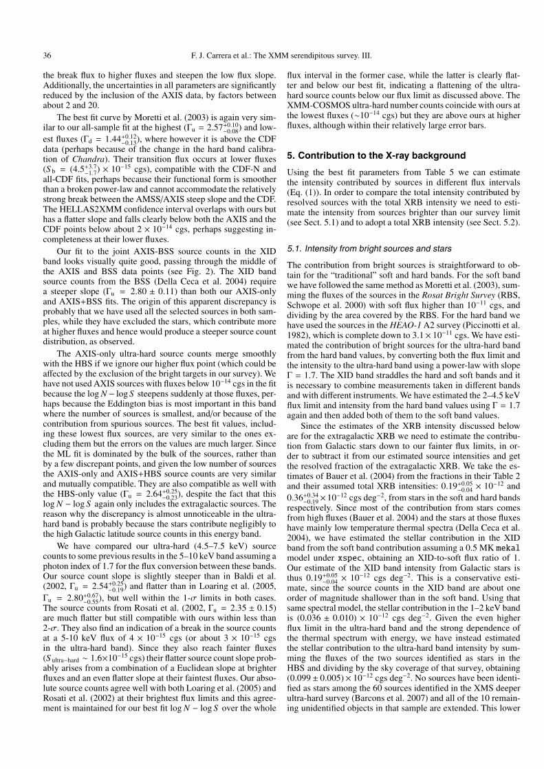
In Fig. 4 we have plotted the relative contribution of twoflux intervals per decade to the total XRB intensity for the four
38 F. J. Carrera et al.: The XMM serendipitous survey. III.
Fig. 4. Relative contribution to the “total” intensity from equally spacedlogarithmic flux intervals using the best fit models in each band (seetext): soft (solid line), hard (dashed), XID (dot-dashed) and ultra-hard(dotted).
default bands, assuming our best fit log N − log S . It is clear thatthe maximum contribution comes from fluxes around the breakflux ∼10−14 cgs. The contribution from the bins in one decadearound that value are close to 50% of the total in the soft andhard bands. In the ultra-hard band we do not reach deep enoughto detect the break. Using the 5–10 keV band source counts ofHasinger et al. (2001) and Rosati et al. (2002) it is possible therecould be a break just below ∼10−14 cgs.
The extrapolation of the soft and hard band log N − log S tozero flux using our best fit model (see Table 6) does not saturatethe XRB intensity, although in the soft band the total XRB inten-sity is within the intensities spanned by the uncertainties in thebest fit log N − log S parameters. This suggests that the possi-bility of a new dominant population at lower fluxes is still open,mainly in the hard band. Under the assumption that the fractionof truly diffuse XRB is negligible (the fluctuation analysis ofMiyaji & Griffiths 2002 shows that the source counts continuegrowing in the soft band down to at least 7 × 10⁻¹⁸ cgs), it ispossible to estimate the minimum slope of the source counts re-quired to just saturate the XRB at zero flux, if the source countssteepened just below the minimum flux studied here. Thoseslopes are 1.85 and 1.84 in the soft and hard bands, respectively.Comparing these values to the observed slopes of the separateAGN and galaxy source counts in the CDF (Bauer et al. 2004),only the absorbed AGN (slope ∼ 1.62, versus 1.2–1.5 for therest of the AGN estimates) come close to being able to saturatethe soft XRB, while galaxies can do so with just about any esti-mate for their source counts slope (2.1–2.7) if they keep grow-ing at the same rate below the resolved fluxes. The situation inthe hard band is also the same, with the absorbed AGN (sourcecounts slope 1.95, versus 1.4–1.5) being the only AGN popula-tion able to contribute the rest of the unresolved intensity, whilethe galaxy source counts estimates (slope 3–3.5) could easilyfulfil this role. A similar conclusion is reached if a higher inten-sity for the XRB is adopted (HM06) since this would steepen thefaint source counts slope required to saturate the XRB.
Even if the source counts re-steepened as discussed in theprevious paragraph, it is clear that the maximum contribution tothe XRB in the soft and hard bands (and probably also in theXID band, and perhaps also in the ultra-hard band) comes fromsources with fluxes within a decade ∼10−14 cgs, where most of
the AXIS sources in those bands lie. This is also true if the XRBintensity is higher than the value used here. Medium depth sur-veys with limiting fluxes close to that value are therefore crucialto understand the evolution of X-rays in the Universe, at leastin the (relatively) soft bands considered here. Sources at lowerfluxes and/or heavily obscured are of course much more impor-tant for the overall energy content of the XRB (Gilli et al. 2001;Fabian & Iwasawa 1999) since they mostly reside in harder X-rays, where the resolved fraction is much smaller (Worsley et al.2004).
5.4. Resolved and unresolved components of the X-raybackground
Comparison between HM06 results and ours (and previous) re-sults involve an uncertainty concerning the different bands un-der consideration (0.5–2 keV vs. 1–2 keV and 2–8 keV vs. 2–10 keV). For the conversions from the 1–2 keV band to the softband and vice versa, as well as the conversions from the 2–8 keVband to the 2–10 keV band, we have assumed power-law photonindices of 1.5 for the unresolved component (as fitted to the un-resolved XRB spectrum by HM06), 1.43 for the resolved faintsources (again as fitted by HM06 to the summed spectrum oftheir resolved sources) and 2 for the resolved sources brighterthan ∼10−14 cgs (Mateos et al. 2005). HM06 have excluded theareas around the sources in Alexander et al. (2003) from theirstudy of the unresolved XRB, with 0.5–2 keV and 2–8 keV fluxlimits of 2.5 × 10⁻¹⁷ and 1.4 × 10⁻¹⁶ cgs respectively. Hence,HM06 define as unresolved any intensity coming from sourcesbelow those flux limits (or from a truly diffuse component).
An additional correction comes from the 2–8 keV band fluxlimits for the resolved sources of HM06, which they take fromAlexander et al. (2003). This same sample was also the basis forthe work of Bauer et al. (2004). We have already seen (Sect. 4.2)that those fluxes need to be decreased by 12% due to a change inthe Chandra calibration, in addition to the correction due to thedifferent bands, as discussed. Assuming a spectral slope of 1.43and taking into account this flux correction, the flux limit in the2–10 keV band becomes 1.6 × 10⁻¹⁶ cgs.
We compare in Table 7 the 0.5–2 keV, 1–2 keV and 2–10 keVX-ray intensity (from different origins and flux intervals) fromHM06 and from the results of this and previous works. The errorbars on our estimates of the intensities have been taken from theerrors on the log N − log S best fit parameters using the standarderror propagation rules (Wall & Jenkins 2003). This has not beenpossible for the extrapolation to zero flux, since the expressionsinvolve the natural logarithm of the lower limit of the interval. Inthis case we have used the values spanned by the uncertaintiesin the best fit log N − log S parameters, as explained in Sect. 4.5.
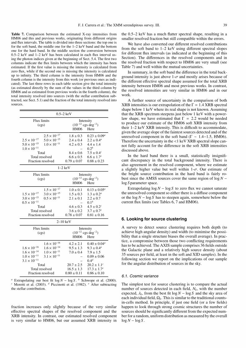
The most noticeable difference is between the total soft XRBintensities, which are not compatible at the ∼1-σ level, while thecorresponding 1–2 keV intensities are compatible at 0.16-σ (seeSect. 5.2). This is because of the very different ways they havebeen obtained: our adopted value is from an extrapolation ofthe Moretti et al. (2003) 1–2 keV total XRB intensity assumingΓ = 1.4, while the HM06 estimate uses different contributionswith different values of the photon index. Since the contributionfrom the brightest sources is almost half of the total and theyhave the steepest spectra, the “effective” spectral slope in theconversion of the HM06 XRB intensity from 1–2 keV to 0.5–2 keV is Γ ∼ 1.72, much steeper than our assumed Γ = 1.4 andhence with a much larger contribution from the 0.5–1 keV inter-val. The HM06 resolved contribution also increases in the softband with respect to the 1–2 keV band, but the resolved
F. J. Carrera et al.: The XMM serendipitous survey. III. 39
Table 7. Comparison between the estimated X-ray intensities fromHM06 and this and previous works, originating from different originsand flux intervals. The table is divided into three sections: the top one isfor the soft band, the middle one for the 1–2 keV band and the bottomone for the hard band. In the middle section the conversion between0.5–2 keV and 1–2 keV has been calculated in each flux interval us-ing the photon indices given at the beginning of Sect. 5.4. The first twocolumns indicate the flux limits between which the intensity has beenestimated. If the first value is missing the intensity is calculated fromzero flux, while if the second one is missing the intensity is calculatedup to infinity. The third column is the intensity from HM06 and thefourth column is the intensity from this work (or previous ones as indi-cated). The last three rows in each table section give the total intensity(as estimated directly by the sum of the values in the third column byHM06 and as estimated from previous works in the fourth column), thetotal intensity resolved into sources (with the stellar contribution sub-tracted, see Sect. 5.1) and the fraction of the total intensity resolved intosources.
0.5–2 keV
Flux limits Intensity(cgs) (10−12 cgs deg−2)
HM06 Here
2.5 × 10⁻¹⁷ 1.8 ± 0.3 0.23 ± 0.09a
2.5 × 10⁻¹⁷ 5.0 × 10⁻¹⁵ 2.4 ± 0.4 2.2 ± 0.4a
5.0 × 10⁻¹⁵ 1.0 × 10⁻¹¹ 4.2 ± 0.3 4.4 ± 1.41.0 × 10−11 – 0.2b
Total 8.4 ± 0.6 7.5 ± 0.4c
Total resolved 6.6 ± 0.5 6.6 ± 1.7e
Fraction resolved 0.79 ± 0.07 0.88 ± 0.23
1–2 keV
Flux limits Intensity(cgs) (10−12 cgs deg−2)
HM06 Here
1.5 × 10⁻¹⁷ 1.0 ± 0.1 0.13 ± 0.05a
1.5 × 10⁻¹⁷ 3.0 × 10⁻¹⁵ 1.5 ± 0.3 1.3 ± 0.2a
3.0 × 10⁻¹⁵ 0.5 × 10⁻¹¹ 2.1 ± 0.1 2.2 ± 0.70.5 × 10−11 – 0.1b
Total 4.6 ± 0.3 4.5 ± 0.2c
Total resolved 3.6 ± 0.2 3.7 ± 0.7e
Fraction resolved 0.78 ± 0.07 0.81 ± 0.16
2–10 keV
Flux limits Intensity(cgs) (10−12 cgs deg−2)
HM06 Here
1.6 × 10⁻¹⁶ 4.2 ± 2.1 0.40 ± 0.04a
1.6 × 10⁻¹⁶ 1.6 × 10⁻¹⁴ 9.5 ± 1.3 9.3 ± 0.4a
1.6 × 10⁻¹⁴ 1.0 × 10⁻¹¹ 7.0 ± 0.4 7.9 ± 1.51.0 × 10−11 3.1 × 10⁻¹¹ – 0.09 ± 0.063.1 × 10−11 – 0.4d
Total 20.7 ± 2.5 20.2 ± 1.1c
Total resolved 16.5 ± 1.3 17.3 ± 1.7e
Fraction resolved 0.80 ± 0.11 0.86 ± 0.10
a Extrapolating our best fit log N − log S . b Schwope et al. (2000).c Moretti et al. (2003). d Piccinotti et al. (1982). e After subtractingthe stellar contribution.
fraction increases only slightly because of the very similareffective spectral shapes of the resolved component and theXRB intensity. In contrast, our estimated resolved componentis very similar to HM06, but our assumed XRB intensity in
the 0.5–2 keV has a much flatter spectral shape, resulting in asmaller resolved fraction but still compatible within the errors.
We have also converted our different resolved contributionsfrom the soft band to 1–2 keV using different spectral slopesfor different flux intervals (as indicated at the beginning of thisSection). The differences in the resolved components and inthe resolved fraction with respect to HM06 are very small (seeTable 7) and well within the mutual uncertainties.
In summary, in the soft band the difference in the total back-ground intensity is just above 1-σ and mostly arises because ofthe different effective spectral shape assumed for the total XRBintensity between HM06 and most previous works. In contrast,the resolved intensities are very similar in HM06 and in ourwork.
A further source of uncertainty in the comparison of bothXRB intensities is our extrapolation of the Γ = 1.4 XRB spectralshape below 1 keV where its real shape is not known. Assumingthat the XRB spectrum steepens just below 1 keV with a power-law shape, we have estimated that Γ = 2.2 would be neededto produce our estimate of the HM06 soft XRB intensity fromtheir 1–2 keV XRB intensity. This is difficult to accommodate,given the average slope of the faintest sources detected and of theunresolved component in the soft band (Γ ∼ 1.4−1.5, HM06).Therefore the uncertainty in the <1 keV XRB spectral slope can-not fully account for the difference in the soft XRB intensitiesdiscussed above.
In the hard band there is a small, statistically insignifi-cant discrepancy in the total background intensity. There isalso agreement in the resolved component, where we estimatea slightly higher value but well within 1-σ. Our estimate ofthe bright source contribution in the hard band is fairly ro-bust since the AMSS sources cover the same region of log N −log S parameter space.
Extrapolating log N − log S to zero flux we cannot saturatethe unresolved component so either there is a diffuse componentor the log N − log S has to steepen again, somewhere below thecurrent flux limits (see Tables 6, 7 and HM06).
6. Looking for source clustering
A survey to detect source clustering requires both depth (toachieve high angular density) and width (to minimise the possi-bility that a single structure biases the overall average). In prac-tice, a compromise between those two conflicting requirementshas to be achieved. The AXIS sample comprises 36 fields outsidethe Galactic plane and a relatively high source density (about35 sources per field, at least in the soft and XID samples). In thefollowing section we report on the implications of our samplefor the angular distribution of sources in the sky.
6.1. Cosmic variance
The simplest test for source clustering is to compare the actualnumber of sources detected in each field, Nk, with the numberexpected, λk, from the best fit log N − log S and the sky area ofeach individual field,Ωk. This is similar to the traditional counts-in-cells method. In principle, if just one field (or a few fields)happen to look through strong cosmic structures the number ofsources should be significantly different from the expected num-ber for a random, uniform distribution as measured by the overalllog N − log S .
40 F. J. Carrera et al.: The XMM serendipitous survey. III.
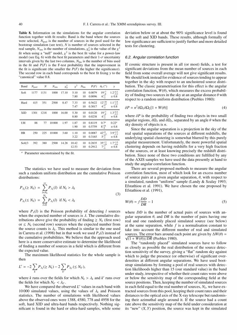
Table 8. Information on the simulations for the angular correlationfunction together with fit results: Band is the band where the sourceswere selected, Npool is the number of sources in the pool used for thebootstrap simulation (see text), N is number of sources selected in thereal sample, Nsim is the number of simulations, χ2
0 is the value of the χ2
fit when using a “null” model, χ2 is the best fit value for a power-lawmodel (see Eq. 6) with the best fit parameters and their 1-σ uncertaintyintervals given by the last two columns, Nbin is the number of bins usedin the fit and P(F) is the F-test probability that the improvement inthe fit is significant (the smaller the P(F) the higher the significance).The second row in each band corresponds to the best fit fixing γ to the“canonical” value 0.8.
Band Npool N Nsim χ20 χ2 Nbin P(F) θ0 (′′) γ
Soft 1177 1131 1000 17.10 5.10 10 0.0079 19+7−8 1.2+0.3
−0.27.80 10 0.0096 6+2
−2 ≡ 0.8
Hard 415 351 2500 8.47 7.33 10 0.5622 12+20−12 1.1+2.8
−2.37.47 10 0.3017 4+5
−4 ≡ 0.8
XID 1301 1218 1000 16.00 5.30 10 0.0120 19+7−8 1.3+0.4
−0.38.80 10 0.0238 4+2
−2 ≡ 0.8
UH 88 77 10 000 1.97 1.87 10 0.8119 0.7a 0.22a
1.90 10 0.5759 8+26−8 ≡ 0.8
HR 250 225 10 000 3.60 1.10 10 0.0087 42+8−12 3.9+2.5
−1.33.22 10 0.3165 5+9
−5 ≡ 0.8
Soft/3 392 380 2500 14.28 10.42 10 0.2835 35+11−18 1.7+1.0
−0.612.53 10 0.2912 7+7
−6 ≡ 0.8
a Parameter unconstrained by the fit.
The statistics we have used to measure the deviation fromsuch a random uniform distribution are the cumulative Poissondistributions:
Pλk (≥ Nk) =∞∑
l=Nk
Pλk (l) if Nk > λk
Pλk (≤ Nk) =Nk∑l=0
Pλk (l) if Nk < λk
(3)
where Pλ(l) is the Poisson probability of detecting l sourceswhen the expected number of sources is λ. The cumulative dis-tributions above give the probability of finding ≥ Nk (first row)or ≤ Nk (second row) sources when the expected number fromthe source counts is λk. This method is similar to the one usedin Carrera et al. (1998) but in that work we used Pλ(l) instead ofthe cumulative probabilities. We believe that the approach usedhere is a more conservative estimate to determine the likelihoodof finding a number of sources in a field which is different fromthe expected value.
The maximum likelihood statistics for the whole sample isthen
L′ = −2∑
k
Pλk (≥ Nk) − 2∑
k′Pλk′ (≤ Nk′ ),
where k runs over the fields for which Nk > λk and k′ runs overthe fields for which Nk′ < λk′ .
We have compared the observed L′ values in each band with10 000 simulated values, using the values of λk and Poissonstatistics. The number of simulations with likelihood valuesabove the observed ones were 1388, 4580, 778 and 4958 for thesoft, hard XID and ultra-hard bands respectively. Nothing sig-nificant is found in the hard or ultra-hard samples, while some
deviation below or at about the 90% significance level is foundin the soft and XID bands. These results, although formally oflow significance are sufficient to justify further and more detailedtests for clustering.
6.2. Angular correlation function
If cosmic structure is present in all (or most) fields, a test forsignificant deviations from the mean number of sources in eachfield from some overall average will not give significant results.We should look instead for evidence of sources tending to appeartogether in the sky with respect to an unclustered source distri-bution. The classic parametrisation for this effect is the angularcorrelation function, W(θ), which measures the excess probabil-ity of finding two sources in the sky at an angular distance θ withrespect to a random uniform distribution (Peebles 1980):
δP = n2δΩ1δΩ2[1 +W(θ)] (4)
where δP is the probability of finding two objects in two smallangular regions, δΩ1 and δΩ2, separated by an angle θ when thesky density of objects is n.
Since the angular separation is a projection in the sky of thereal spatial separations of the sources at different redshifts, theunderlying spatial clustering is somewhat blurred by this purelyangular measurement. Unfortunately, the more powerful spatialclustering depends on having redshifts for a very high fractionof the sources, or at least knowing precisely the redshift distri-bution. Since none of these two conditions are fulfilled by anyof the AXIS samples we have used the data presently at hand tostudy the angular correlation function.
There are several proposed methods to measure the angularcorrelation function, most of which look for an excess numberof source pairs at a given angular separation, θ, with respect toa simulated, random “uniform” sample (Landy & Szalay 1993;Efstathiou et al. 1991). We have chosen the one proposed byEfstathiou et al. (1991),
W(θ) = fDDDR− 1 (5)
where DD is the number of actual pairs of sources with an-gular separation θ, and DR is the number of pairs having onereal and one randomly placed simulated source (see below)at the same separation, while f is a normalisation constant totake into account the different number of real and simulatedsources. The error bars around each point are given by ∆W(θ) =√
(1 +W(θ))/DR (Peebles 1980).The “randomly placed” simulated sources have to follow
as closely as possible the real distribution of the source detec-tion sensitivity of the survey, giving a “flat” random sky againstwhich to judge the presence (or otherwise) of significant over-densities at different angular separations. We have used boot-strap simulations by forming a pool of real sources with detec-tion likelihoods higher than 15 (our standard value) in the bandunder study, irrespective of whether their count rates were aboveor below the sensitivity map of the corresponding field at thesource positions. Then, keeping the number of simulated sourcesin each field equal to the real number of sources, Nk, we have ex-tracted sources from this pool, keeping their count rates and theirdistances to the optical axis of the X-ray telescope but randomis-ing their azimuthal angle around it. If the source had a countrate above the sensitivity map of the field under consideration atits “new” (X, Y) position, the source was kept in the simulated
F. J. Carrera et al.: The XMM serendipitous survey. III. 41
sample, otherwise a new one is extracted until Nk valid simu-lated sources are found. In this way, the angular distribution ofthe simulated sources mimics the decline of the source detectionsensitivity with off-axis angle. The number of random samplesNsim used in each band are shown in Table 8. They have beenchosen so as to give a total of about a million simulated sourcesin each band.
Using this recipe, the normalisation constant f above is givenby
f =∑
k Nk (Nk − 1)
2Nsim∑
k N2k
,
Nk being the number of sources in field k and Nsim is the numberof simulations.
If a positive correlation is present at angular scales compara-ble to the individual field size then the estimate of the mean sur-face density of objects from the survey is too high and this causesa negative bias in the angular correlation function known as theintegral constraint (Basilakos et al. 2004). Given the complicateddependence of the sensitivity over the area of our survey we havecorrected for this effect empirically, finding the angular correla-tion function that we would have detected in the absence of cor-relation via the average of Nsim simulated realisations of W(θ),where the real data were replaced by random samples simulatedindependently following the recipe in the previous paragraph.The triangles in Fig. 5 show these “zero points” at each angularscale which have been used to increase the corresponding ob-served W(θ), convolving the error bars using Gaussian statistics.
Applying Eq. (5) to the full sample results in a ∼3-σ signif-icant bump at about 200 arcsec, which was also present in thesimulations but at lower significance. The bump turned out to bepresent in only two fields, HD 111812 and HD 117555. A searchin the literature revealed that both fields have stellar clusters intheir field of view (Eggen & Iben 1989). Since we are mainly in-terested in extragalactic structure we have opted to exclude thesetwo fields from all subsequent angular clustering analysis, leav-ing 34 fields.
The W(θ) values obtained in this fashion are shown in Fig. 5as well as the corresponding best χ2 fits to a power-law model
W(θ) = (θ/θ0)−γ. (6)
The best fit parameters for this model are given in Table 8. Inthis Table we also give the significance of the detection froman F-test, comparing the χ2 value of the power-law model witha simple W(θ) = 0, no-clustering model. The F-test suggestssignificant correlation in the soft and XID bands at the ∼99%level. The lack of significant detections in the two harder bandsmight be due to the lower number of sources with respect to thesoft and XID bands (see below).
Gandhi et al. (2006) also found significant angular correla-tion in the XMM-LSS sample in the soft band with a similarslope, γ = 1.2±0.2, and a lower correlation length, θ0 = 7±3 arc-sec, but still compatible with our result within ∼1-σ. Vikhlinin& Forman (1995) found γ = 0.7 ± 0.3 and θ0 = 4 ± 3 arc-sec, again a lower correlation length than our results, but com-patible within less than 1-σ with our γ ≡ 0.8 result. On theother hand, Basilakos et al. (2005) also found significant angu-lar correlation in this band but with a higher correlation length,θ0 = 10.4 ± 1.9 arcsec (with the canonical slope), just com-patible with our results at about the 2-σ level. Basilakos et al.(2005) also used Limber’s equation (Peebles 1980) to calcu-late the spatial correlation function from the angular correla-tion function, assuming several different AGN X-ray luminos-ity functions (since most X-ray sources at low flux levels are
expected to be AGN). Their high correlation lengths are onlycompatible with AGN optical (e.g. Croom et al. 2002; Grazianet al. 2004) or X-ray correlation functions (Carrera et al. 1998;Akylas et al. 2000; Mullis et al. 2004) if the clustering is constantin physical coordinates, while optical QSO clustering seems in-stead to be constant in comoving coordinates (Croom et al. 2001,but see also Grazian et al. 2004 and Croom et al. 2005). Akylaset al. (2000) also found significant angular correlation in the softband sources in the RASS-BSC, but at much higher angular dis-tances (∼8).
Correlation of hard band selected sources is not detected byGandhi et al. (2006) (413 sources) and Puccetti et al. (2006)(205 sources). However, clustering is very significantly detected(>4σ) by Basilakos et al. (2004) (171 sources) with γ = 1.2±0.3and θ0 = 49+16
−25 arcsec. Clustering is also detected at similar sig-nificance by Yang et al. (2003), with θ0 = 40 ± 11 arcsec (forγ ≡ 0.8) for 278 sources. This is somewhat surprising sincethe Basilakos et al. sample has less than half of the numberof sources in Gandhi et al., and a similar number of sources toPuccetti et al., while the Yang et al. sample is again smaller thanthe Gandhi et al. sample. Our angular correlation length is com-patible with the Basilakos et al. (2004) (and with the Puccettiet al.) result within 1-σ, but not with the Yang et al. correlationlength. However, the F-test on the correlation function and thesuperior Pλ(N) test (see below and Fig. 6) do not detect clus-tering. Again, our sample seems to give somewhat intermediateresults in between those of Basilakos et al. (2004) and Yang et al.(2003) on one hand and Gandhi et al. (2006) and Puccetti et al.(2006) on the other.
Since each bin in W(θ) contains information from manypairs, perhaps involving the same real and simulated sourcesmany times, it is at least debatable whether the hypothesis ofindependent bins underlying the χ2 test applies in this case. Tocircumvent this problem we have applied a simple test for thesignificance of the correlation, using Poisson statistics to com-pare the expected number of pairs (at distances smaller or equalthan each individual observed distance) in the absence of corre-lation (µ =
∑θ′<θ DR(θ′)/ f ) with the number of observed pairs
(Nθ =∑θ′<θ DD(θ′)). The quantity 1 − Pµ(Nθ) versus the angu-
lar distance θ is shown in Fig. 6 for each band. We estimatedthe “signal” in the absence of correlation in a similar way tothe method used to quantify the integral constraint but here re-placing the real data by randomly placed sources (see above).For each sample we have performed 10 000 simulations in thismanner. Hence, for each angular scale and sample we have de-termined the distribution of the expected value of 1 − Pµ(Nθ) ifthe sources are not correlated. We show in Fig. 6 the median andthe upper 99% and 99.9% percentiles of those distributions foreach angular scale. The simulations show clearly that the detec-tion significance is actually lower than the value given purely byPoisson statistics, when there are more than ∼1000 sources, as inthe soft and XID bands where the 99% percentile is at around thePoisson 3-σ level. In the hard and ultra-hard bands the 99% per-centile is close to the “right” Poisson position, albeit with largeexcursions.
Using the percentile values from the simulations we havefound a >99% (but mostly <99.9%) significant detection of cor-relation in the angular positions in our soft sample at separations200–700 arcsec. In the XID band the significance is lower, at justabout 99% significance, with essentially one peak of higher sig-nificance at ∼300 arcsec. In contrast, no signal is found in eitherthe hard or ultra-hard bands. The lack of significant detectionsin the two harder bands might be due to the lower number ofsources with respect to the soft and XID bands.

42 F. J. Carrera et al.: The XMM serendipitous survey. III.
Fig. 5. W(θ) vs. θ for the soft (top-left), hard (top-right), XID (middle-left), and ultra-hard (middle-right) samples, for a hardness-ratio selectedsample (bottom-left) and for a random selection of one third of the soft sources (bottom-right). The solid dots are the integral constraint-correctedobserved values, the grey triangles show the “zero points” from the integral constraint (displaced to the left for clarity) and the solid lines are thebest fit χ2 fits to Eq. (6). The middle-right and two bottom panels have different scales on their Y-axis.
We have tested the influence of the number of sources onthe detection of clustering, since we only detect clustering in thesamples with more than 1000 sources. We rejected at randomtwo of every three sources in the soft band sample and repeatedboth correlation tests and found that the clustering signal disap-pears (see Table 8, Figs. 5 and 6). We also repeated this test whilekeeping at random half and two thirds of the soft sources, only
finding correlation at the 99% level in the last case. We concludethat clustering in the hard and ultra-hard bands may be as strongor stronger than clustering in the soft band but our relatively lownumber of sources prevents us from detecting it. This is consis-tent with the results of Gilli et al. (2005) who do not find anysignificant difference between the clustering properties of soft orhard X-ray selected sources in the CDF.

F. J. Carrera et al.: The XMM serendipitous survey. III. 43
Fig. 6. 1 − Pµ(Nθ) vs. θ for the soft (top-left), hard (top-right), XID (middle-left), ultra-hard (middle-right) selected samples, for a hardness-ratioselected sample (bottom-left) and for a random selection of one third of the soft sources (bottom-right). The median (50%), 99% and 99.9% levelsfrom random simulations are also shown (grey jagged lines). The Y-axis scaling is different in each panel and has been chosen for maximumclarity.
The significant clustering found for the Pµ(Nθ) in the softband corresponds to a broad bump between about 150 and700 arcsec with “peaks” at about 300, 400 and 650 arcsec (thefirst two are significant even at the 99.9% level). These “peaks”also appear to be present in the XID band. While the increase inthe number of real pairs giving rise to the broad bump is verygradual, the “peaks” must correspond to significant increases in
relatively narrow ranges of angular distances. To investigate ifthese “peaks” come from a small number of fields in a particularregion of the sky we divided the sample between the fields inthe northern and southern Galactic hemispheres. The 1− Pµ(Nθ)relation for these regions are shown in Fig. 7. Despite the lowersignificance of the results (expected because of the lower num-bers of sources), the broad bump and peaks are still present in

44 F. J. Carrera et al.: The XMM serendipitous survey. III.
Fig. 7. 1−Pµ(Nθ) vs. θ for the soft band and for the fields in the northern (left) and southern (right) Galactic hemispheres. The median (50%), 99%and 99.9% levels from random simulations are also shown (grey jagged lines).
the samples from each hemisphere with the ∼300 arcsec peakbeing common to both. The peak at 400 arcsec appears pre-dominantly in the northern hemisphere and the peak at 650 arc-sec occurs in the southern hemisphere. We have also repeatedthe analysis while excluding the two fields with obvious clus-ter emission (A1837 and A399) from the northern and southernGalactic hemisphere sub-samples respectively, finding no signif-icant differences in the strength or position of the “peaks”. As afurther test, we have looked for this signal in the 7 deeper fields(Texp > 40 ks, ∼400 sources) and in the remaining 27 fields(∼800 sources), finding significant correlation only in the lattercase and hence the signal is not introduced by a few deep fields.
A detailed discussion of the (cosmic or statistical) origin ofthese structures is outside the scope of this paper and will be dis-cussed using a larger sample in a future paper. However, what-ever the origin of the angular structure we have found, it mustbe relatively widespread over the survey area and/or the sky. Wetake this to mean that, if it has a real cosmic origin it must comefrom sources at z ≤ 1.5, which is the peak of the redshift distri-bution of medium depth X-ray surveys (Barcons et al. 2007).
6.3. Angular correlation of a hardness ratio selected sampleof sources
A low significance or absence of correlation in the hard bandis somewhat surprising since most sources at the flux levels ofour sample are AGN (Barcons et al. 2007), which are knownto cluster strongly (both X-ray selected, Mullis et al. 2004;Yang et al. 2006, and optically selected, Croom et al. 2005).Furthermore, obscured AGN appear more commonly in hard X-ray selected samples (Della Ceca et al. 2006; Caccianiga et al.2004; Della Ceca et al. 2004; Barcons et al. 2007).
Gandhi et al. (2006) have found that, despite the absence ofsignificant angular correlation in their hard sample, if they se-lect only the hardest spectrum sources (using the soft-to-hardhardness ratio) and they use lower significance sources, the sig-nificance of their correlation increases to ∼2−3σ. They loweredtheir significance level in order to increase the number of sourcesin the tested sample. This significant correlation in only the hard-est of the hard X-ray selected sources is a very intriguing andpotentially interesting result.
We have performed a similar analysis, defining the samehardness ratio HR = (H − S )/(H + S ) where H and S are the
2–12 keV and 0.5–2 keV count rates respectively. We have se-lected the sources detected in either the soft or hard bands (inthe sense explained in Sect. 2.4) which have HR ≥ −0.2 (Gandhiet al. 2006).
The F-test seems to indicate correlation at >99% level(Table 8), but the superior Poisson method (Fig. 5) does not de-tect clustering on any angular scales, with the data being con-sistent with the median of the random simulations. We cannotthus confirm the results of Gandhi et al. (2006), despite havinga slightly larger sample of sources (250 versus their 209). Thisis consistent with the results of Yang et al. (2006) who do notfind any significant differences between the spatial clustering ofsources with soft or hard spectra.
7. Conclusions
We present the results from AXIS (An XMM-NewtonInternational Survey), which comprises 1433 distinct serendip-itous X-ray sources detected above a likelihood of 15 (∼5-σ)in XMM-Newton EPIC pn observations in 36 different XMM-Newton observations at high Galactic latitude. We have definedsub-samples in four bands: 0.5–2 keV(soft, 1267 sources), 2–10 keV (hard, 397 sources), 0.5–4.5 keV (XID, 1359 sources)and 4.5–7.5 keV (ultra-hard, 91 sources). The first two being the“standard” X-ray bands, the third one chosen to span the energyrange with the best sensitivity of that camera and the last onetaking advantage of the unprecedented hard X-ray sensitivity ofXMM-Newton above 4 keV. Given the distribution of exposuretimes of the fields selected for AXIS it will serve as a pathfinderfor the X-ray and optical properties of the sources in large scaleXMM-Newton catalogues (1XMM, 2XMM, . . .).
Using count rates in the 5 standard XMM-Newton bands aslow-resolution spectra we have fitted single power-laws to allsources in the XID and hard bands independently, in order to cal-culate source fluxes without assuming a constant spectrum (seeTable 4). Our internal and external checks make us confident ofthe results using this technique. The average best fit power-lawslope in the XID band is 〈Γ〉 ∼ 1.8, independent of the sample towhich the sources belong, while the average is 〈Γ〉 ∼ 1.5−1.6 inthe hard band.
We have constructed empirical sensitivity maps in all fourbands taking into account the exposure maps, the backgroundmaps and the excluded regions (see Table 1). We have derived

F. J. Carrera et al.: The XMM serendipitous survey. III. 45
sky coverage as a function of flux in each of these four bands,taking into account the distribution of spectral slopes of thesources. The total area covered is 4.8 deg2 (see Fig. 1).
Our data have been combined with both wider and shal-lower (BSS/HBSS, Della Ceca et al. 2004, AMSS, Ueda et al.2005) and narrower and deeper (CDF, Bauer et al. 2004) sur-veys to measure the X-ray source counts over as wide a fluxrange as possible, reaching 4 orders of magnitude in the softband (∼2000 sources), ∼3 in the hard and XID bands (∼800 and∼1800 sources, respectively) and a bit more than 1 in the (largelyunexplored) ultra-hard band (∼140 sources). The data from dif-ferent observatories and instruments are mutually compatible soallowing a joint analysis of the source counts.
We have performed maximum likelihood fits to a brokenpower-law model for the log N − log S in each of the four bands(see Table 5). We have found that fits to the source counts usingfixed spectral slopes produce similar results to those using indi-vidual source spectral slopes (as we have done here) but give riseto larger error bars. The source counts in the soft, hard and XIDbands show breaks at fluxes ∼10−14 cgs. Detailed examinationof the ratios between the data and this simple model in the softand XID band do not show any significant differences, while inthe hard band there seems to be evidence for a further flux breakat ∼3 × 10⁻¹⁵ cgs and several changes of slope. Since this isonly present in the hard band, it is difficult to assess whetherthis behaviour is due to an over simple characterisation of con-tributions from different populations at different redshifts or tocalibration uncertainties. Future large scale XMM-Newton cata-logues (such as 2XMM) will be useful for addressing this ques-tion. The best fit model parameter values are compatible withprevious smaller or similar surveys, but our combination of largenumber of sources and wide flux coverage produce in generalsmaller uncertainties in the best fit parameters.
We have used our best fit log N − log S parameters to cal-culate both the total resolved fraction of the XRB (includingthe contribution from sources at bright fluxes, see Table 6) andthe relative contribution of different flux bins to the XRB (seeFig. 4). We have used the estimates of the average XRB inten-sity in the soft and hard bands from Moretti et al. (2003) andtranslated them to the XID and ultra-hard bands using Γ = 1.4(Marshall et al. 1980). The total resolved fraction down to thelowest fluxes of the combined sample reaches 87% in the softband and 85% in the hard band, where we have been able toreach deep fluxes using pencil beam surveys (Bauer et al. 2004),but is only ∼60% in the XID band and about 25% in the ultra-hard band. The total intensity produced by extrapolating our bestfit soft and hard log N − log S to zero flux is insufficient to satu-rate the XRB intensity. Assuming a second flux break just belowour minimum detected fluxes, we have estimated the minimumslope below this break necessary to reproduce the whole XRBwith discrete sources, obtaining 1.85 (1.84) in the soft (hard)band. Comparing these slopes with those of the fainter galaxyand AGN source counts from the CDF (Bauer et al. 2004), weshow that galaxies could easily provide this re-steepening, whileamong AGN only perhaps the absorbed cases could possiblydo so.
The maximum fractional contribution to the XRB in the soft,hard and XID bands comes from sources within a decade of10−14 cgs (which is about where the break flux for the brokenpower-law occurs). This fractional contribution reaches about50% of the total in the soft and hard bands. Medium depth sur-veys such as AXIS (and indeed the 1XMM catalogue and itssuccessor 2XMM) are therefore crucial to understand the evolu-tion of the X-ray emission in the Universe, at least up to 10 keV.
Hickox & Markevitch (2006) have recently re-estimated thesoft and hard XRB intensities using CDF data, finding lower re-solved fractions of the XRB than our (and previous) estimates.We have found that the difference between our results in thesoft band (where it is highest) is only at the ∼1-σ level and ismainly due to the different ways in which the total XRB inten-sity is calculated. HM06 add different contributions at differentfluxes, which produces an “effective” spectral shape of the XRB(Γ ∼ 1.8) which is much steeper than the “canonical” XRB spec-tral slope of Γ = 1.4 (which we have assumed). We have shownthat the difference between these estimates of the soft XRB in-tensity cannot be removed just by relaxing our assumption. TheHM06 intensity from resolved sources is very similar to ours.Converting our results to 1–2 keV the difference with HM06 allbut vanishes.
After excluding two fields in which there is evidence for thepresence of stellar clusters we used the AXIS sources to studythe presence of cosmological structure in the X-ray sky, throughthe cosmic variance in the number of sources per field and thedistribution of the angular separations of the sources. The for-mer is in principle more sensitive to the presence of significantover-densities in a few fields while the latter detects any overallangular clustering of sources. No cosmic variance is detected atall in the hard and ultra-hard bands while some signal at aboutthe 90% level is present in the soft and XID bands, probablybecause they are the ones with the larger number of sources.
Angular clustering is studied in two ways. The first is theangular correlation function, W(θ). Using this method we detectsignal at about the 99% level in the soft and XID bands but not inthe hard and ultra-hard bands (Table 8 and Fig. 5). The strengthof the clustering signal we have found is intermediate betweenthose of previous results (e.g. Gandhi et al. 2006; Basilakos et al.2004, 2005; Vikhlinin & Forman 1995). Formally, a more ap-propriate method using Poissonian statistics detects clustering atthe 99–99.9% level in the soft and XID samples, but not in thehard or ultra-hard bands (Fig. 6). Repeating the test for a ran-dom, 1-in-3 selected sample of soft sources completely removesthe clustering signal, which we take to imply that there might bea “real” angular clustering among hard sources which we havefailed to detect due to the smaller number of sources. Dividingthe soft sample into several sub-samples reveals that the signal iswidespread over the sky and not limited to a few deep fields. Thismeans that if it has a cosmic origin it must come from z ≤ 1.5,the peak of the redshift distribution of medium flux X-ray sur-veys (Barcons et al. 2007). We cannot confirm the detection ofa signal among hard-spectrum hard sources reported by Gandhiet al. (2006).
Acknowledgements. This research has made use of the NASA/IPACExtragalactic Database (NED; which is operated by the Jet PropulsionLaboratory, California Institute of Technology, under contract with the NationalAeronautics and Space Administration) and of the SIMBAD database (operatedby CDS, Strasbourg, France). Financial support for this work was provided bythe Spanish Ministerio de Educación y Ciencia under projects ESP2003-00812and ESP2006-13608-C02-01. This research has made use of the USNO-A2.0catalogue, maintained at the U.S. Naval Observatory. SM, MP, MW, JT and SRacknowledge financial support for this research from PPARC. RDC and TMreceived partial financial support from the Italian Space Agency under contractASI-INAF n. I/023/05/0.
References
Akylas, A., Georgantopoulos, I., & Plionis, M. 2000, MNRAS, 318, 1036Alexander, D., Bauer, F. E., Brandt, W. N., et al. 2003, AJ, 126, 539Arnaud, K. 1996, Astronomical Data Analysis Software and Systems V., ed. G.
Jacoby, & J. Barnes, ASP Conf. Ser., 101, 17Baldi, A., Molendi, S., Comastri, A., et al. 2002, ApJ, 564, 190

46 F. J. Carrera et al.: The XMM serendipitous survey. III.
Barcons, X., Mateos, S., & Ceballos, M. T. 2000, MNRAS, 311, 456Barcons, X., Carrera, F. J., Watson, M. G., et al. 2002, A&A, 382, 522Barcons, X., Carrera, F. J., & Ceballos, M. T. 2006, ESA-SP, 604, 789Barcons, X., Carrera, F. J., et al. 2007, submitted to A&ABasilakos, S., Georgakakis, A., Plionis, M., & Georgantopoulos, I. 2004, ApJ,
607, L79Basilakos, S., Plionis, M., Georgakakis, A., & Georgantopoulos, G. 2005,
MNRAS, 356, 183Bauer, F. E., Alexander, D. M., Brandt, W. N., et al. 2004, AJ, 128, 2048Caccianiga, A., Severgnini, P., Braito, V., et al. 2004, A&A, 416, 901Cagnoni, I., Della Ceca, R., & Maccacaro, T. 1998, ApJ, 493, 54Cappelluti, N., Hasinger, G., Brusa, M., et al. 2007, ApJS, in press
[arXiv:astro-ph/0701196]Carrera, F. J., Barcons, X., Fabian, A. C., et al. 1998, MNRAS, 299, 229Civano, F., Comastri, A., & Brusa, M. 2005, MNRAS, 358, 693Cowie, L. L., Garmire, G. P., Bautz, M. W., et al. 2002, ApJ, 566, L5Croom, S. M., Shanks, T., Boyle, B. J., et al. 2001, MNRAS, 325, 483Croom, S. M., Boyle, B. J., Loaring, N. S., et al. 2002, MNRAS, 335, 459Croom, S. M., Boyle, B. J., Shanks, T., et al. 2005, MNRAS, 356, 415De Luca, A., & Molendi, S. 2004, A&A, 419, 837Della Ceca, R., Castelli, G., Braito, V., Cagnoni, I., & Maccacaro, T. 1999, ApJ,
524, 674Della Ceca, R., Maccacaro, T., Caccianiga, A., et al. 2004, A&A, 428, 383Della Ceca, R., Caccianiga, A., Severgnini, P., et al. 2006, ESA-SP, 604, 783Dickey, J. M., & Lockman, F. J. 1990, ARA&A, 28, 215Eddington, A. S. 1913, MNRAS, 73, 359Efstathiou, G., Bernstein, G., Tyson, J. A., Katz, N., & Guhathakurta, P. 1991,
ApJ, 380, L47Eggen, O. J., & Iben, I. 1989, AJ, 97, 431Ehle, M., Breitfellner, M., González-Riestra, R., et al. 2005, XMM-Newton
Users’ Handbook, ESAFabian, A. C., & Barcons, X. 1992, ARA&A, 30, 429Fabian, A. C., & Iwasawa, K. 1999, MNRAS, 303, L34Gabriel, C., Denby, M., Fyfe, D. J., et al. 2004, in Astronomical Data Analysis
software and Systems XIII, ed. F. Ochsensbein, M. Allen, & D. Egret, ASPConf. Ser., 314, 759
Gandhi, P., Garcet, O., Disseau, L., et al. 2006, A&A, 457, 393Giacconi, R., Gursky, H., Paolini, F. R., & Rossi, B. B. 1962, Phys. Rev. Lett., 9,
439Giacconi, R., Rosati, P., Tozzi, P., et al. 2001, ApJ, 551, 624Giacconi, R., Zirm, A., Wang, J., et al. 2002, ApJS, 139, 369Gilli, R., Salvati, M., & Hasinger, G. 2001, A&A, 366, 407Gilli, R., Daddi, E., Zamorani, G., et al. 2005, A&A, 430, 811Grazian, A., Negrello, M., Moscardini, L., et al. 2004, AJ, 127, 592Hasinger, G., Burg, R., Giacconi, R., et al. 1998, A&A, 329, 482
Hasinger, G., Altieri, B., Arnaud, M., et al. 2001, A&A, 365, L45Hasinger, G., Cappelluti, N. Brunner, H., et al. 2007, ApJS, in press
[arXiv:astro-ph/0612311]Hickox, R. C., & Markevitch, M. 2006, ApJ, 645, 95Hornschemeier, A. E., Bauer, F. E., Alexander, D. M., et al. 2003, AJ, 126, 575Kim, D.-W., Cameron, R. A., Drake, J. J., et al. 2004, ApJS, 150, 19La Franca, F., Fiore, F., Comastri, A., et al. 2005, ApJ, 635, 864Landy, S. D., & Szalay, A. 1993, ApJ, 412, 64Loaring, N., Dwelly, T., Page, M. J., et al. 2005, MNRAS, 362, 1371Lumb, D. H., Warwick, R. S., Page, M., & De Luca, A. 2002, A&A, 389, L93Marshall, F. E., Boldt, E. A., Holt, S. S., et al. 1980, ApJ, 235, 4Mateos, S., Barcons, X., Carrera, F. J., et al. 2005, A&A, 433, 855Miyaji, T., & Griffiths, R. E. 2002, ApJ, 564, L5Moretti, A., Campana, S., Lazzati, D., & Tagliaferri, G. 2003, ApJ, 588, 696Mullis, C. R., Henry, J. P., Gioia, I. M., et al. 2004, ApJ, 617, 192Page, M. J., Mittaz, J. P. D., & Carrera, F. J. 2000, MNRAS, 318, 1073Peebles, P. J. E. 1980, The large-scale structure of the universe (Princeton
University Press), 435Piccinotti, G., Mushotzky, R. F., Boldt, E. A., et al. 1982, ApJ, 253, 485Pierre, M., Valtchanov, I., Altieri, B., et al. 2004, J. Cosm. Astropart. Phys., 9,
11Puccetti, S., Fiore, F., D’Elia, V., et al. 2006, A&A, 457, 501Rosati, P., Tozzi, P., Giacconi, R., et al. 2002, ApJ, 566, 667Schwope, A., Hasinger, G., Lehmann, I., et al. 2000, AN, 321, 1Setti, G., & Woltjer, L. 1989, A&A, 224, L21Sołtan, A. 1982, MNRAS, 200, 115Strüder, L., Briel, U., Dennerl, K., et al. 2001, A&A, 365, L18Tedds, J. A., Page, M. J., et al. 2007, in preparationTurner, M. J. L., Abbey, A., Arnaud, M., et al. 2001, A&A, 365, L27The First XMM-Newton Serendipitous Source Catalogue, XMM-Newton
Survey Science Centre, 2003 (http://xmmssc-www.star.le.ac.uk/)Ueda, Y., Akiyama, M., Ohta, K., & Miyaji, T. 2003, ApJ, 598, 886Ueda, Y., Ishisaki, Y., Takahashi, T., Makishima, K., & Ohashi, T. 2005, ApJS,
161, 185Ueda, Y., et al. 2007, in preparationVikhlinin, A., & Forman, W. 1995, ApJ, 455, L109Vikhlinin, A., Forman, W., Jones, C., & Murray, S. 1995, ApJ, 451, 564Wall, J. V., & Jenkins, C. R. 2003, Practical Statistics for Astronomers
(Cambridge University Press)Worsley, M. A., Fabian, A. C., Barcons, X., et al. 2004, MNRAS, 352, l28Worsley, M. A., Fabian, A. C., Bauer, F. E., et al. 2006, MNRAS, 368, 1735Yang, Y., Mushotzky, R. F., Barger, A. J., et al. 2003, ApJ, 585, L85Yang, Y., Mushotzky, R. F., Barger, A. J., & Cowie, L. L. 2006, ApJ, 645, 68Zamorani, G. Gioia, I. M., Maccacaro, T., & Wolter, A. 1988, A&A, 196, 39

F. J. Carrera et al.: The XMM serendipitous survey. III., Online Material p 1
Online Material
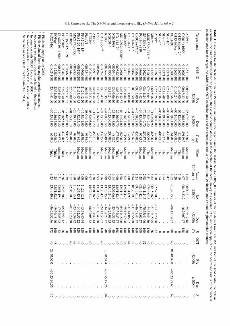
F. J. Carrera et al.: The XMM serendipitous survey. III., Online Material p 2
Table1.
Basic
datafor
the36
fields
inthe
AX
ISsurvey:
includingthe
targetnam
e,the
XM
M-N
ewton
OB
S_ID
number
ofthe
pndataset
used,the
RA
andD
ecof
thefi
eldcentre,
the“clean”
exposuretim
eand
thefi
lterused
forthe
pncam
era,theG
alacticcolum
ndensity
inthe
directionof
thefi
eld(D
ickey&
Lockm
an1990)
and,where
applicable,thecentre
andradius
ofthe
circularexclusion
areafor
thetarget,the
width
ofthe
OO
Texclusion
areaand
thecentre
andradius
ofan
additionalexclusionarea
aroundbright/extended
sources.
Targetname
OB
S_ID
RA
Dec
Texp
Filter
NH,G
alR
AD
ecR
OO
TR
AD
ecR′
(J2000)(J2000)
(s)(10
20cm−
2)(J2000)
(J2000)(”)
(”)(J2000)
(J2000)(”)
A2690
012531010100:00:30.30
−25:07:30.00
21586.7M
edium1.84
00:00:21.2−
25:08:12.1820
0-
-0
Cl0016
+1609
a0111000101
00:18:33.00+
16:26:18.0029149.3
Medium
4.0700:18:33.2
+16:26:07.97
1480
--
0G
133-69pos_2a
011265050101:04:00.00
−06:42:00.00
18080.0T
hin5.19
--
00
--
0G
133-69Pos_1
a0112650401
01:04:24.00−
06:24:00.0020000.0
Thin
5.20-
-0
0-
-0
PH
L1092
011089050101:39:56.00
+06:19:21.00
16180.0M
edium4.12
01:39:55.8+
06:19:19.6788
4001:40:09.0
+06:23:27.67
68S
DS
-1ba,d
011237100102:18:00.00
−05:00:00.00
43040.0T
hin2.47
--
00
--
0S
DS
-3a,d
011237150102:18:48.00
−04:39:00.00
14927.9T
hin2.54
--
00
--
0S
DS
-2a,d
011237030102:19:36.00
−05:00:00.00
40673.0T
hin2.54
--
00
--
0A
399a,c
011226020102:58:25.00
+13:18:00.00
14298.7T
hin11.10
02:57:50.2+
13:03:20.88272
0-
-0
Mkn3
a,c
011122020106:15:36.30
+71:02:04.90
44506.1M
edium8.82
06:15:36.6+
71:02:15.9576
32-
-0
MS
0737.9+
7441a,e
012310020107:44:04.50
+74:33:49.50
20209.3T
hin3.51
07:44:04.3+
74:33:54.56120
40-
-0
S5
0836+
71a
011262010108:41:24.00
+70:53:40.70
25057.3M
edium2.98
08:41:24.3+
70:53:41.06160
52-
-0
PG
0844+
3490103660201
08:47:42.30+
34:45:04.909783.5
Medium
3.2808:47:42.9
+34:45:03.27
20040
--
0C
l0939+
4713a
010646010109:43:00.10
+46:59:29.90
43690.0T
hin1.24
09:43:01.8+
46:59:44.37160
0-
-0
B21028
+31
a0102040301
10:30:59.10+
31:02:56.0023236.0
Thin
1.9410:30:59.3
+31:02:56.08
14072
--
0B
21128+
31a
010204020111:31:09.40
+31:14:07.00
13799.8T
hin2.00
11:31:09.6+
31:14:06.02140
44-
-0
Mkn205
a,e
012411010112:21:44.00
+75:18:37.00
17199.6M
edium3.02
12:21:43.8+
75:18:39.08140
36-
-0
MS
1229.2+
6430a,e
012490010112:31:32.32
+64:14:21.00
28700.0T
hin1.98
12:31:31.2+
64:14:18.06140
40-
-0
HD
111812b
000822020112:50:42.56
+27:26:07.70
37338.8T
hick0.90
12:51:42.6+
27:32:23.27168
40-
-0
NG
C4968
000294010113:07:06.10
−23:40:43.00
4898.7M
edium9.14
13:07:06.3−
23:40:33.2340
0-
-0
NG
C5044
003795010113:15:24.10
−16:23:06.00
20030.0M
edium5.03
13:15:24.2−
16:23:08.53340
0-
-0
IC883
009364040113:20:35.51
+34:08:20.50
15849.4M
edium0.99
13:20:35.4+
34:08:21.3748
013:20:54.4
+33:55:17.26
104H
D117555
a,b
010024020113:30:47.10
+24:13:58.00
33225.4M
edium1.16
13:30:47.8+
24:13:51.07160
40-
-0
F278
006194010113:31:52.37
+11:16:48.70
4648.3T
hin1.93
13:31:52.4+
11:16:43.8848
0-
-0
A1837
a0109910101
14:01:34.68−
11:07:37.2045361.3
Thin
4.3814:01:36.5
−11:07:43.14
4400
--
0U
ZL
iba
010024080115:32:23.00
−08:32:05.00
23391.2M
edium8.97
15:32:23.4−
08:32:05.32140
40-
-0
FieldV
I0067340601
16:07:13.50+
08:04:42.009634.0
Medium
4.00-
-0
0-
-0
PK
S2126-15
a0103060101
21:29:12.20−
15:38:41.0016150.0
Medium
5.0021:29:12.1
−15:38:40.44
12040
--
0P
KS
2135-14a,f
009285020121:37:45.45
−14:32:55.40
28484.3M
edium4.70
21:37:45.1−
14:32:55.22120
44-
-0
MS
2137.3-23530008830101
21:40:15.00−
23:39:41.009880.0
Thin
3.5021:40:15.1
−23:39:39.32
14048
--
0P
B5062
a0012440301
22:05:09.90−
01:55:18.1028340.9
Thin
6.1722:05:10.3
−01:55:20.38
14040
--
0L
BQ
S2212-1759
a0106660101
22:15:31.67−
17:44:05.0090892.5
Thin
2.39-
-0
0-
-0
PH
L5200
a0100440101
22:28:30.40−
05:18:55.0043278.5
Thick
5.2622:28:30.4
−05:18:53.12
160
--
0IR
AS
22491-1808a
008134090122:51:49.49
−17:52:23.20
19867.2M
edium2.71
22:51:49.4−
17:52:25.0232
0-
-0
EQ
Peg
a0112880301
23:31:50.00+
19:56:17.0012200.0
Thick
4.2523:31:52.7
+19:56:18.46
16048
--
0H
D223460
010024100123:49:41.00
+36:25:33.00
6699.0T
hick8.25
23:49:40.8+
36:25:32.56172
4023:50:02.0
+36:25:36.36
116
aF
ieldsbelonging
tothe
XM
S.
bF
ieldsexcluded
fromthe
angularcorrelation
studies.ceposcorr
astrometric
correctionfailed
inthese
fields.
dIn
comm
onw
ithS
XD
S(U
edaetal.2006).
eIn
comm
onw
ithH
EL
LA
S2X
MM
(Baldietal.2002).
fS
ame
areaas
oneC
haMP
field
(Kim
etal.2004).
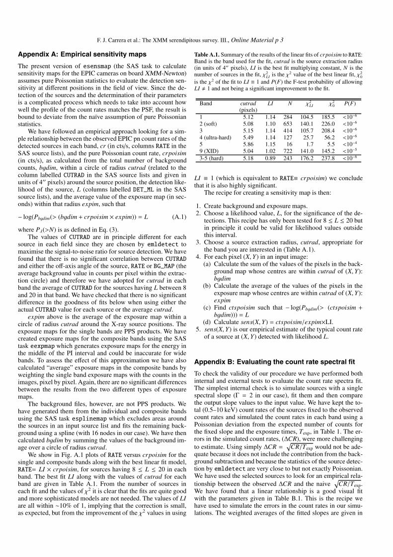
F. J. Carrera et al.: The XMM serendipitous survey. III., Online Material p 3
Appendix A: Empirical sensitivity maps
The present version of esensmap (the SAS task to calculatesensitivity maps for the EPIC cameras on board XMM-Newton)assumes pure Poissonian statistics to evaluate the detection sen-sitivity at different positions in the field of view. Since the de-tection of the sources and the determination of their parametersis a complicated process which needs to take into account howwell the profile of the count rates matches the PSF, the result isbound to deviate from the naïve assumption of pure Poissonianstatistics.
We have followed an empirical approach looking for a sim-ple relationship between the observed EPIC pn count rates of thedetected sources in each band, cr (in cts/s, columns RATE in theSAS source lists), and the pure Poissonian count rate, crpoisim(in cts/s), as calculated from the total number of backgroundcounts, bgdim, within a circle of radius cutrad (related to thecolumn labelled CUTRAD in the SAS source lists and given inunits of 4′′ pixels) around the source position, the detection like-lihood of the source, L (columns labelled DET_ML in the SASsource lists), and the average value of the exposure map (in sec-onds) within that radius expim, such that
− log(Pbgdim(> (bgdim + crpoisim × expim)) = L (A.1)
where Pλ(>N) is as defined in Eq. (3).The values of CUTRAD are in principle different for each
source in each field since they are chosen by emldetect tomaximise the signal-to-noise ratio for source detection. We havefound that there is no significant correlation between CUTRADand either the off-axis angle of the source, RATE or BG_MAP (theaverage background value in counts per pixel within the extrac-tion circle) and therefore we have adopted for cutrad in eachband the average of CUTRAD for the sources having L between 8and 20 in that band. We have checked that there is no significantdifference in the goodness of fits below when using either theactual CUTRAD value for each source or the average cutrad.
expim above is the average of the exposure map within acircle of radius cutrad around the X-ray source positions. Theexposure maps for the single bands are PPS products. We havecreated exposure maps for the composite bands using the SAStask eexpmap which generates exposure maps for the energy inthe middle of the PI interval and could be inaccurate for widebands. To assess the effect of this approximation we have alsocalculated “average” exposure maps in the composite bands byweighting the single band exposure maps with the counts in theimages, pixel by pixel. Again, there are no significant differencesbetween the results from the two different types of exposuremaps.
The background files, however, are not PPS products. Wehave generated them from the individual and composite bandsusing the SAS task esplinemap which excludes areas aroundthe sources in an input source list and fits the remaining back-ground using a spline (with 16 nodes in our case). We have thencalculated bgdim by summing the values of the background im-age over a circle of radius cutrad.
We show in Fig. A.1 plots of RATE versus crpoisim for thesingle and composite bands along with the best linear fit model,RATE= LI × crpoisim, for sources having 8 ≤ L ≤ 20 in eachband. The best fit LI along with the values of cutrad for eachband are given in Table A.1. From the number of sources ineach fit and the values of χ2 it is clear that the fits are quite goodand more sophisticated models are not needed. The values of LIare all within ∼10% of 1, implying that the correction is small,as expected, but from the improvement of the χ2 values in using
Table A.1. Summary of the results of the linear fits of crpoisim to RATE:Band is the band used for the fit, cutrad is the source extraction radius(in units of 4′′ pixels), LI is the best fit multiplying constant, N is thenumber of sources in the fit, χ2
LI is the χ2 value of the best linear fit, χ20
is the χ2 of the fit to LI ≡ 1 and P(F) the F-test probability of allowingLI 1 and not being a significant improvement to the fit.
Band cutrad LI N χ2LI χ2
0 P(F)(pixels)
1 5.12 1.14 284 104.5 185.5 <10−6
2 (soft) 5.08 1.10 653 140.1 226.0 <10−6
3 5.15 1.14 414 105.7 208.4 <10−6
4 (ultra-hard) 5.49 1.14 127 25.7 56.2 <10−6
5 5.86 1.15 16 1.7 5.5 <10−4
9 (XID) 5.04 1.02 722 141.0 145.2 <10−5
3-5 (hard) 5.18 0.89 243 176.2 237.8 <10−6
LI ≡ 1 (which is equivalent to RATE≡ crpoisim) we concludethat it is also highly significant.
The recipe for creating a sensitivity map is then:
1. Create background and exposure maps.2. Choose a likelihood value, L, for the significance of the de-
tections. This recipe has only been tested for 8 ≤ L ≤ 20 butin principle it could be valid for likelihood values outsidethis interval.
3. Choose a source extraction radius, cutrad, appropriate forthe band you are interested in (Table A.1).
4. For each pixel (X, Y) in an input image:(a) Calculate the sum of the values of the pixels in the back-
ground map whose centres are within cutrad of (X, Y):bgdim
(b) Calculate the average of the values of the pixels in theexposure map whose centres are within cutrad of (X, Y):expim
(c) Find ctspoisim such that − log(Pbgdim(> (ctspoisim +bgdim))) = L
(d) Calculate sens(X, Y) = ctspoisim/expim×LI.5. sens(X, Y) is our empirical estimate of the typical count rate
of a source at (X, Y) detected with likelihood L.
Appendix B: Evaluating the count rate spectral fit
To check the validity of our procedure we have performed bothinternal and external tests to evaluate the count rate spectra fit.The simplest internal check is to simulate sources with a singlespectral slope (Γ = 2 in our case), fit them and then comparethe output slope values to the input value. We have kept the to-tal (0.5–10 keV) count rates of the sources fixed to the observedcount rates and simulated the count rates in each band using aPoissonian deviation from the expected number of counts forthe fixed slope and the exposure times, Texp, in Table 1. The er-rors in the simulated count rates, (∆CR), were more challengingto estimate. Using simply ∆CR =
√CR/Texp would not be ade-
quate because it does not include the contribution from the back-ground subtraction and because the statistics of the source detec-tion by emldetect are very close to but not exactly Poissonian.We have used the selected sources to look for an empirical rela-tionship between the observed ∆CR and the naive
√CR/Texp.
We have found that a linear relationship is a good visual fitwith the parameters given in Table B.1. This is the recipe wehave used to simulate the errors in the count rates in our simu-lations. The weighted averages of the fitted slopes are given in

F. J. Carrera et al.: The XMM serendipitous survey. III., Online Material p 4
Fig. A.1. RATE vs. crpoisim for all bands. Also shown are the best linear fits.
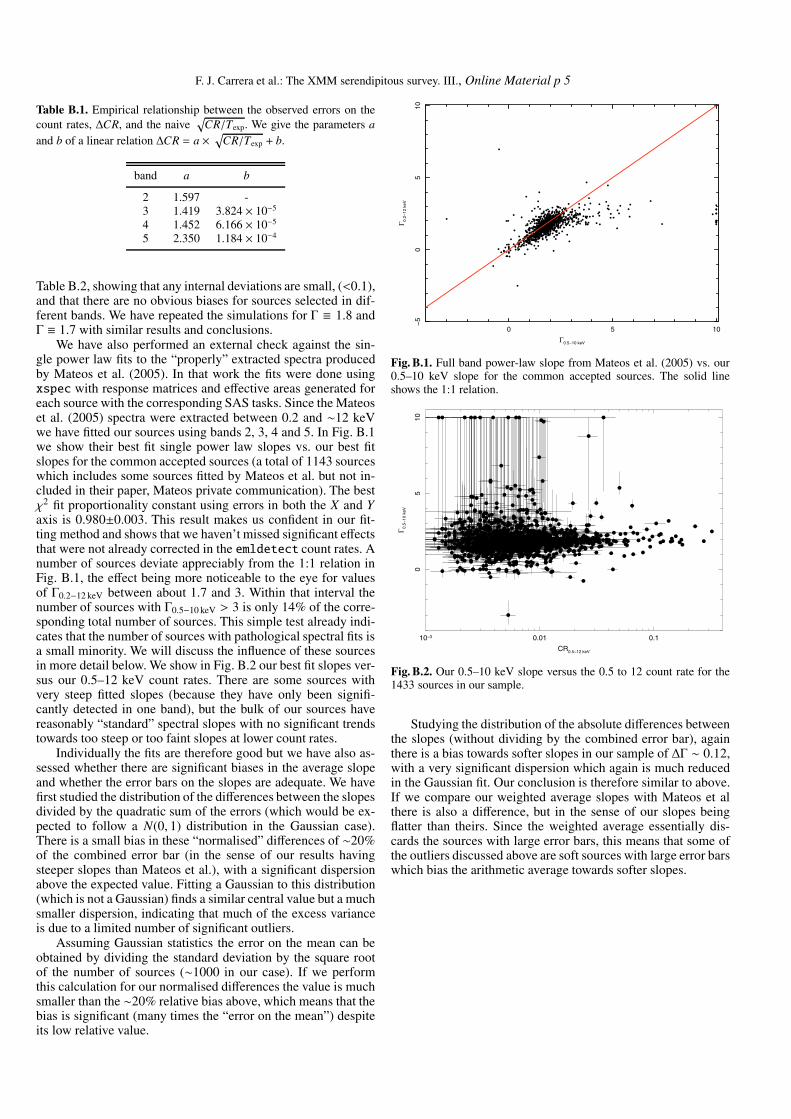
F. J. Carrera et al.: The XMM serendipitous survey. III., Online Material p 5
Table B.1. Empirical relationship between the observed errors on thecount rates, ∆CR, and the naive
√CR/Texp. We give the parameters a
and b of a linear relation ∆CR = a × √CR/Texp + b.
band a b
2 1.597 -3 1.419 3.824 × 10⁻⁵
4 1.452 6.166 × 10⁻⁵
5 2.350 1.184 × 10⁻⁴
Table B.2, showing that any internal deviations are small, (<0.1),and that there are no obvious biases for sources selected in dif-ferent bands. We have repeated the simulations for Γ ≡ 1.8 andΓ ≡ 1.7 with similar results and conclusions.
We have also performed an external check against the sin-gle power law fits to the “properly” extracted spectra producedby Mateos et al. (2005). In that work the fits were done usingxspec with response matrices and effective areas generated foreach source with the corresponding SAS tasks. Since the Mateoset al. (2005) spectra were extracted between 0.2 and ∼12 keVwe have fitted our sources using bands 2, 3, 4 and 5. In Fig. B.1we show their best fit single power law slopes vs. our best fitslopes for the common accepted sources (a total of 1143 sourceswhich includes some sources fitted by Mateos et al. but not in-cluded in their paper, Mateos private communication). The bestχ2 fit proportionality constant using errors in both the X and Yaxis is 0.980±0.003. This result makes us confident in our fit-ting method and shows that we haven’t missed significant effectsthat were not already corrected in the emldetect count rates. Anumber of sources deviate appreciably from the 1:1 relation inFig. B.1, the effect being more noticeable to the eye for valuesof Γ0.2−12 keV between about 1.7 and 3. Within that interval thenumber of sources with Γ0.5−10 keV > 3 is only 14% of the corre-sponding total number of sources. This simple test already indi-cates that the number of sources with pathological spectral fits isa small minority. We will discuss the influence of these sourcesin more detail below. We show in Fig. B.2 our best fit slopes ver-sus our 0.5–12 keV count rates. There are some sources withvery steep fitted slopes (because they have only been signifi-cantly detected in one band), but the bulk of our sources havereasonably “standard” spectral slopes with no significant trendstowards too steep or too faint slopes at lower count rates.
Individually the fits are therefore good but we have also as-sessed whether there are significant biases in the average slopeand whether the error bars on the slopes are adequate. We havefirst studied the distribution of the differences between the slopesdivided by the quadratic sum of the errors (which would be ex-pected to follow a N(0, 1) distribution in the Gaussian case).There is a small bias in these “normalised” differences of ∼20%of the combined error bar (in the sense of our results havingsteeper slopes than Mateos et al.), with a significant dispersionabove the expected value. Fitting a Gaussian to this distribution(which is not a Gaussian) finds a similar central value but a muchsmaller dispersion, indicating that much of the excess varianceis due to a limited number of significant outliers.
Assuming Gaussian statistics the error on the mean can beobtained by dividing the standard deviation by the square rootof the number of sources (∼1000 in our case). If we performthis calculation for our normalised differences the value is muchsmaller than the ∼20% relative bias above, which means that thebias is significant (many times the “error on the mean”) despiteits low relative value.
0 5 10
−5
05
10
Γ 0.2−
12 k
eV
Γ0.5−10 keV
Fig. B.1. Full band power-law slope from Mateos et al. (2005) vs. our0.5–10 keV slope for the common accepted sources. The solid lineshows the 1:1 relation.
10−3 0.01 0.1
05
10
Γ 0.5−
10 k
eV
CR0.5−12 keV
Fig. B.2. Our 0.5–10 keV slope versus the 0.5 to 12 count rate for the1433 sources in our sample.
Studying the distribution of the absolute differences betweenthe slopes (without dividing by the combined error bar), againthere is a bias towards softer slopes in our sample of ∆Γ ∼ 0.12,with a very significant dispersion which again is much reducedin the Gaussian fit. Our conclusion is therefore similar to above.If we compare our weighted average slopes with Mateos et althere is also a difference, but in the sense of our slopes beingflatter than theirs. Since the weighted average essentially dis-cards the sources with large error bars, this means that some ofthe outliers discussed above are soft sources with large error barswhich bias the arithmetic average towards softer slopes.
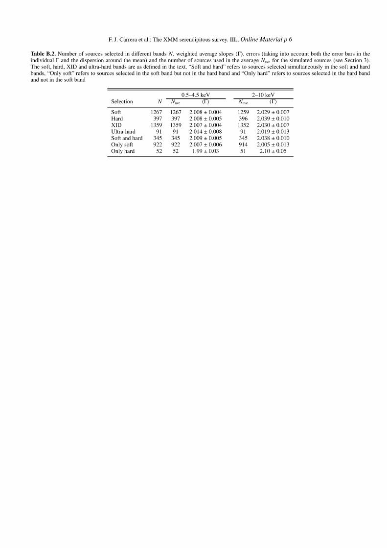
F. J. Carrera et al.: The XMM serendipitous survey. III., Online Material p 6
Table B.2. Number of sources selected in different bands N, weighted average slopes 〈Γ〉, errors (taking into account both the error bars in theindividual Γ and the dispersion around the mean) and the number of sources used in the average Nave for the simulated sources (see Section 3).The soft, hard, XID and ultra-hard bands are as defined in the text. “Soft and hard” refers to sources selected simultaneously in the soft and hardbands, “Only soft” refers to sources selected in the soft band but not in the hard band and “Only hard” refers to sources selected in the hard bandand not in the soft band
0.5–4.5 keV 2–10 keVSelection N Nave 〈Γ〉 Nave 〈Γ〉Soft 1267 1267 2.008 ± 0.004 1259 2.029 ± 0.007Hard 397 397 2.008 ± 0.005 396 2.039 ± 0.010XID 1359 1359 2.007 ± 0.004 1352 2.030 ± 0.007Ultra-hard 91 91 2.014 ± 0.008 91 2.019 ± 0.013Soft and hard 345 345 2.009 ± 0.005 345 2.038 ± 0.010Only soft 922 922 2.007 ± 0.006 914 2.005 ± 0.013Only hard 52 52 1.99 ± 0.03 51 2.10 ± 0.05