1

Thematic map accuracy assessment of Pool 8, Upper Mississippi River: A pilot study. Mara S. May1,2

1Department of Resource Analysis, St. Mary’s University of Minnesota, Winona, MN 55987 2U. S. Geological Survey, Upper Midwest Environmental Services Center, Onalaska, WI 54603 Keywords: Land cover maps, Pool 8, spatial accuracy, producer accuracy, thematic accuracy assessment, Upper Mississippi River, user accuracy Abstract Land cover/ land use maps provide valuable information to a variety of users. Accuracy assessments determine how useful these maps are to the user. A thematic accuracy assessment was designed and implemented for the vector-based 2001 land cover/ land use dataset for Pool 8 of the Upper Mississippi River. The dataset was created from 1:15,000-scale Color InfraRed (CIR) aerial photography flown in late summer 2001. A stratified random sampling design was implemented based on the dominant land cover classes. Coordinates were generated for sample points using a random point generator for each stratum or land cover class. Fieldwork on the river was completed between September 2001 and March 2002. The total number of sample points used for analysis was 514. The overall accuracy was calculated to be 83.8%. Producer and user accuracies varied according to the class and are reported with 90% confidence limits. The dataset was collapsed into a more generalized classification based on hydrology, and the overall accuracy was calculated to be 88.5%; and producer and user accuracies are reported with 90% confidence limits. Key issues with accuracy assessment are discussed, including assessor limitations and variability in photo-interpretation. Recommendations for future assessments are made based upon the results of this study. Introduction Thematic maps produced with the technology of geographical information systems (GIS) have enormous potential to provide detailed information to the users of the map. Key to the usefulness of a map for any user is the degree of quality, or accuracy, of the map (Congalton 1991; Stehman and Czaplewski 1998; Story and Congalton 1986). To quantify the accuracy of a map, thematic accuracy assessments can be completed to determine the probability of which classified map types do not conform to the ground truth or reference data (Congalton 1991; Story and Congalton 1986). Accuracy assessments have received a lot of attention in the literature during the last fifteen years, and they remain a

prominent topic because of the potential of satellite-derived image datasets and the widespread use of computer GIS (Moisen et al. 2000). Statistically sound designs for accuracy assessments have been addressed as well (Moisen et al. 2000; Stehman and Czaplewski 1998). Regardless of the scope or size of the project, however, the actual procedure of thematic accuracy assessments remains fundamentally unchanged.

Thematic maps may have data derived from ground plots or other ground data sources, interpreted aerial photographs, satellite images, or any combination of the above. Maps derived from photointerpreted land cover contain some areas that are classified with greater confidence (or certainty), such as structures or open water boundaries, and other areas that are

2

classified with more variability (or uncertainty). These areas are more variable because most vegetation does not have clearly demarked boundaries from one community or association to the next (Lowell and Edwards 1996). Before photo-interpretation begins, the photointerpreter will spend time ground-truthing -- examining photo signatures against field observations-- in order to reduce classification error and to increase consistency in interpreting the cover types correctly. However, the photointerpreter must still be guided from what can be seen on the aerial photograph. Inevitably, variation in interpretation, even among experienced photointerpreters, arises in areas of greater heterogeneity, in areas of coarser resolution, and in areas where vegetation signatures can be easily confused (Congalton 1991; Lowell and Edwards 1996). Thus, from the map producer perspective, a thematic accuracy assessment would provide invaluable information about the degree of correctness of a map’s classification.

A thematic accuracy assessment is geared primarily to static systems, to maps that are not anticipated to change from one year to the next. A principle assumption of accuracy assessments is that the reference data, usually collected by the assessor in the form of plot data, is the ‘truth’ when compared to the map classification. This assumption has been reported in the literature as a critical factor in accuracy assessments (Congalton 1991; Stehman and Czaplewski 1998). Since the late 1990s, staff from the National Park Service (NPS) mapping program at the Upper Midwest Environmental Sciences Center in La Crosse, Wisconsin (UMESC) has developed custom error justification lists with the vegetation maps they produce. These descriptions are essential in showing key limitations in the vegetation classification,

map production, and accuracy assessment processes.

Maps produced by UMESC for the Upper Mississippi River are designed for many uses. Management decision making for habitat restoration, designing protected areas for waterfowl nesting and staging, and examining trends in land cover over time are examples that all rely upon accurate information. The accuracy of the dataset is important to both the producer and the users of the data. In 2001, a study was initiated at UMESC to examine the process of thematic map accuracy assessment and its applicability to a river system. The assessment of maps for dynamic systems like rivers is just in the beginning stages. The assessment team for this study determined which components of an accuracy assessment are needed in order to examine the land cover /land use (LCU) maps in a timely manner.

This pilot study describes the method used for assessing the thematic accuracy of the 2001 LCU map produced by UMESC. Error matrices are reported and discussed for both a detailed and a more generalized map classification. Finally, a series of recommendations is provided to generate a cost-effective means of conducting regular accuracy assessments for LCU maps. Methods Data sources, sampling design, and sample point selection Two LCU vector coverages for Pool 8 of the Upper Mississippi River, years 2000 and 2001, were used for this study. These datasets were provided by UMESC. Both datasets were photo-interpreted at a scale of 1:15,000. Each coverage was classified (or mapped) by a different photointerpreter. Quality control was performed by the same person on both coverages to check the

3

linework and attributes. The minimum mapping unit was defined as half a hectare (approximately one acre), and vegetation was mapped to the genus level where possible.

Points were chosen as the most appropriate and practical sampling unit for examining the accuracy of a moderate-sized map (Environmental Systems Research Institute et al. 1994; Congalton 1991; Stehman and Czaplewski 1998). Each LCU class to be assessed was assigned a certain number of sampling points (Table 1).

Table 1. Guidelines used for number of points to sample for each LCU class.

This strategy was a modification of the recommendations for point-based sampling which originated with the NPS vegetation mapping projects (Environmental Systems Research Institute et al. 1994). The total number of potential sampling points was 561.

A stratified random sampling design was employed for this study. The 2000 LCU coverage was subsetted in UNIX-ArcInfo 8.0. Polygons in the 2000 coverage that were less than half a hectare (the size of the minimum map unit) were excluded from the assessment because of the likelihood of spatial error accessing these small areas. The coverage was assessed to the genus level, so the “UMR_ATT” attribute class in the Polygons Attribute Table (PAT) were used excluding all modifiers. To expedite the assessment, a query removed all LCU polygons that were designated “developed” or “urban”. These areas were removed

primarily because the accuracy of identifying developed areas is seldom an issue for producers or for users. The remaining LCU classes were aggregated based on the single dominant genus. Each polygon was re-assigned an attribute in an item labeled ‘GENUS’. For example, all polygons that were dominated by Nymphaea (Ny), such as Ny-Sagittaria, Ny-Nelumbo, and Ny-Submerged Vegetation, were assigned the GENUS label ‘Ny’. Marsh categories were an exception to this aggregation. In instances where particular emergent species generally grew at deeper depths monotypically than when mixed with other species, marsh classes were created. These marsh classes were created for Sagittaria, Sparganium, Typha, and Zizania. A total of 37 GENUS classes were identified (Appendix 1). Within each GENUS class, a subset was generated and the polygons were buffered inside and outside to 10 meters to offset the effects of Global Positioning System (GPS) errors and ecotones.

The sampling points were generated per GENUS class using a random-grid Arc Macro Language (AML) program produced by UMESC. The arc tool rndgrid rasterized a coverage and used a 25 meter cell size. This cell size was well below the minimum map unit to accommodate the potential for more points in smaller polygons. The arc tool is dependent on the item “STRATA” in the PAT to identify into which polygons to place points. Between one and three points per polygon was permitted per GENUS class depending upon the size and shape of the polygons.

Field data collection

Reference data were collected on day trips between September 2001 and March 2002. Aquatic sampling points, prioritized by the

Number of polygons per LCU class Number of points

to assign 30 or more 30

20 to 29 20 10 to 19 10 1 to 9 All

4

persistence of the vegetation being assessed, were accessed by outboard motorboat or by airboat. Wading to reach the correct coordinates was often necessary. Terrestrial sampling points were accessed either by land or by boat. Garmin 3+ recreational receivers, either depth sounder units or hand-held units, were used to locate each point. Coordinates were projected in datum NAD27 Universal Transverse Mercator (UTM) Zone 15 to match the projection used in the LCU maps. Sample point X-Y coordinates, the estimated error of position (EPE), and the Dilution of Precision (DOP) were recorded.

When the sample point was in deep water and drift occurred, the coordinates for the point were accepted within 5 to 20 meters of the point. When the sample point was in shallow water or on land, the coordinates were taken between 0 and 5 meters of the sample point’s designated coordinates. Depths were recorded to the nearest decimeter and were determined either by reading the Garmin depth sounder or by using measuring stakes.

The assessor had simple maps with only polygon boundaries on them to reference in which direction to describe the vegetation. The assessor visually plotted a 50 X 50 meter squared area and described the vegetation within the plot. The shape of the “plot” was meant to be contained wholly within the polygon to be sampled. The recorder (when a second staff was present) or the assessor took notes on the general characteristics of the plot and, on many occasions, other vegetation existing near the plot. The dominant GENUS class evident to the assessor was recorded (this is termed a “field call” or reference classification). Normally, some descriptive information and percent-cover estimates were also documented, but in some instances no additional information was recorded. Taking digital photographs of each plot was

added to the protocol beginning in November; these images were catalogued according to the code number assigned to each sampling point.

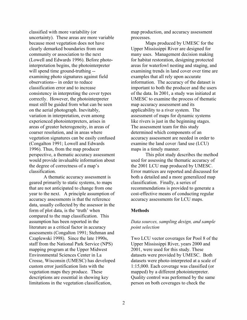
A total of 514 points (194 aquatic and 320 terrestrial points) were sampled, representing 39 GENUS classes in the 2001 dataset (Figure 1).

Nearly all sections of the pool were sampled for at least one GENUS class. The field component was completed in 38 field days and involved five staff and one intern during different times of sampling. One main investigator made 431 field calls (covering 37 GENUS classes); a second team made 88 other calls (covering 19 GENUS classes). The difference in the number of GENUS classes actually used (39) and the number that was stratified (37) was due to the use of additional map classes. One GENUS class, Echinochloa, was present in 2001 in mappable quantities but was not present in the 2000 land cover/ land use dataset. The second class was ‘DV’, or ‘developed’,

$

$

$$$$

$$$$

$$

$

$$$$ $

$$$

$

$$$

$$$$$

$$$

$$

$

$$$$

$$$$$$$$$

$

$$$$$$

$$$$$ $

$$

$

$

$$$ $

$$

$$

$

$$$$$ $$$$$$

$$$$

$$$

$$$$$ $

$

$

$

$$$

$$

$$$$

$$

$ $

$

$$$$$$$$

$$

$$$$$$

$$$

$$$$

$$$

$

$$ $ $$$$

$

$ $$$$

$$$$ $

$$ $

$$

$$$$$$$

$

$

$$$

$$

$$

$

$$$

$

$$

$$$$$

$

$

$

$

$$$$

$$

$$$ $$

$$

$ $$$

$$$

$$$$$

$$

$$$$

$$$$$$$

$$$$$$$$

$$$$$$

$$$$$$$$

$$

$$$$

$

$$

$$ $ $$$$

$

$

$

$$

$$$$

$

$

$$ $ $

$$

$$ $

$

$$

$$$

$$$$$

$$$

$

$

$$

$

$

$

$$

$

$$

$

$ $

$

$

$

$$$

$

$$

$

$$

$

$

$

$$$

$$

$

$

$

$

$

$$$

$$

$

$

$

$

$$$

$$$$ $

$$$$ $

$$

$$$$$

$$$$ $$$$$$$$$$

$$

$

$$

$

$$$$$$$$$$

$$

$

$

$$$

$

$$

$

$

$

$

$

$

$$

$

$$

$$

$$$$

$$

$$$$$$$

$

$

$

$$$ $ $

$

$

$

$

$$

$

$

$$$

$$$

$

$$$

$$$$$

$$$$$

$

$$

$

$$

$

$$

$$$$

$$

$$

$$

$

$

$$

$

$

$$

$$

$

$$$

$$$$$$

$

Pool 8LandWater

Developed areas$ Sample points

LEGEND

3 0 3 6 Kilometers

Genoa, WI

Onalaska, WI

La Crescent, MN

Figure 1. Pool 8 of the Upper Mississippi River with all points sampled from the 2001 accuracy assessment.

5

which an assessor used to describe the area at a sample point even though the accuracy assessment was meant to exclude developed and urban land cover classes. Post field data assessment: defining sources of error The field assessment data were transcribed to a Microsoft Access database and were checked for transcription errors. The file was then imported into ArcView 3.2, where the point coordinates and identifying code were joined spatially to polygon attributes from the 2001 LCU map. The spatial join was a one-to-one relationship, meaning that one, and only one GENUS class from the reference data (each sample point) could be matched with one and only one GENUS class from the map classification. This new dataset was exported directly to Microsoft Excel. There, the data were separated into an ‘initial match’ or ‘initial mismatch’ category. ‘Initial matches’ were any sample points that had the same dominant GENUS type as the map classification. ‘Initial mismatches’ were any sample points that did not have the same dominant GENUS type as the map classification. Mismatches occur in an accuracy assessment for many reasons. The classification system, the automation process, and the reference data may all contribute error to the assessment. Because maps generalize reality, it is tremendously difficult to create an all-encompassing, mutually exclusive classification system for all land types without splitting every type into an unusable number of categories (Lowell and Edwards 1996). Thus, classifications are created that have some very specific land cover classes and other more heterogeneous classes. Distinctive signatures must be identified for each land cover class. If a land cover type is heterogeneous in nature, signatures may be

less distinct and more prone to variable photo-interpretation. Areas with substantial heterogeneity in the vegetation may be classified similarly because of the signature (Owens and Hop 1995). However, the perspective from the assessor on the ground may be quite different, and grasping the heterogeneity correctly using a standard sample point is difficult. Thus, a mismatch may arise between the classification data and the reference data, but the mismatch may be due to heterogeneity of the site, and not to a mis-classification or an incorrect field call. The photointerpretation and automation procedures may also introduce error into a map and thus into the assessment. Photointerpreters may be limited in delineation, due to photography and to signature limitations (Lowell and Edwards 1996). Thus, a mismatch may occur in areas where the photointerpreter has no real way of determining what exists at a particular location. The transfer from mylar to digital data may introduce some spatial error. Shifts in the tens of meters can result in sample points not being located within the polygon which was assessed, and this may result in mismatches even though the true classification data and the references data are the same. Errors in the assessment procedure include mis-identification of land cover types and errors in location (GPS errors) among others. For example, if an assessor records GPS coordinates that are inaccurate, then the reference data point and the classification for that area will not overlay correctly, and a mismatch will occur. These three areas may result in mismatches that are not truly in error if further investigations are made. If the mismatches remain without examination, a lower overall accuracy may result, incorrectly reducing the confidence in the map’s quality.

6

k =

The assessor’s reference data produced 272 initial matches and 243 initial mismatches on the 2001 classified LCU dataset. Mismatches were the primary order of concern for the assessment team, and they were examined first.

Categories of explanations were developed to help the group differentiate between the different types of error. ArcView 3.2 was used to display the sample points. The imagery used included 1:12,000 –scale digital orthophoto quarter quadrangles (DOQQ) of Pool 8 (based upon early 1990’s aerial photography), and available georeferenced photo-mosaics of the pool (flown in July and August 2001). The data sheets, digital photographs taken in the field, and original aerial photographs were also used for reference. During this review, data provided in the assessor’s field sheet and on the 2001 photo-mosaics were used to examine the discrepancies. Occasionally, the original aerial photograph was examined to affirm or to refute a field or a photointerpreter’s classification. If a reasonable and valid explanation could be made to match the sample point and the map classification, then the assessment for that point was considered correct and the GENUS class was updated as necessary. Parameters were set by the assessment team to distinguish between these ‘false’ errors and true errors, errors for which no agreement could be reached. When a mismatched point was examined and no valid reason existed for matching the map classification and the reference sample point, the point was assigned as a final mismatch. Most of the sample points (171) that initially matched (272 sample points) were overlaid on 2001 partial photo-mosaics of Pool 8 in ArcView. Screen captures were taken of each sample point and the available 2001 photo-mosaic. This process helped to determine if the same types of errors that

were identified in the mismatches also existed for sample points that were initially matches. Questionable areas were brought to the group for final assessment. No sample points examined contained errors that would result in reference or classified data being changed. The final ‘match’ and ‘mismatch’ datasets were combined for analysis. Data analysis A confusion matrix (also called an error matrix or a contingency table) was generated to calculate the overall thematic accuracy and the producer and user accuracies for the 2001 LCU map (Congalton 1991, Stehman and Czaplewski 1998, Story and Congalton 1986). A confusion matrix “represents a contingency table in which the diagonal entries represent correct classification or agreement between the map and reference data, and the off-diagonal entries represent misclassifications, or lack of agreement between the map and the reference data” (Stehman and Czaplewski 1998). The unadjusted accuracy was calculated by summing the diagonal entries and dividing the sum by the total number of points sampled.

Overall accuracy was adjusted to eliminate the possibility of chance agreement by using a kappa index (Environmental Systems Research Institute et al. 1994; Congalton 1991). The computational formula is as follows:

Pcorrect - Pchance

1 - Pchance Pcorrect “the proportion of correctly classified entries” Pchance “the proportion of samples expected to be classified correctly by chance”, where Pchance = Σ Prow(i) – Pcolumn(j) P row(i) is the proportion of total entries in row i Pcolumn(j) is the proportion of total entries in column j

7

To build the confusion matrix, selected fields were queried using a crosstab query in Access on the assessor’s adjusted reference data and the adjusted map classification. The query was exported as a Dbase V file into Excel for further analysis and for data formatting. The results were reported verbally for clarity rather than in the traditional contingency table.

Producer accuracy was measured to describe the accuracy of the map from the perspective of the people producing the map. Producer accuracy was calculated by taking the number of matches for a particular GENUS class and dividing it by the total number of reference samples identified for that class. Confidence limits at 90% were also calculated to estimate the limits of confidence for each individual producer accuracy value (Environmental Systems Research Institute et al. 1994).

User accuracy responds to the question of “how well the map represents what is really on the ground” (Story and Congalton 1986). User accuracy was calculated by taking the number of matches for a particular GENUS class and dividing that value by the total number of sample points classified by the photointerpreter. Confidence limits were set at 90% for each value.

After this analysis was completed, the reference dataset was collapsed to a more generalized category of classes using the UMR_GEN or 31-classification attribute (Appendix 1). This classification system is used frequently by researchers for analysis. Two classes in this classification, Deep Marsh Perennial (DMP) and Shallow Marsh Perennial (SMP), were aggregated to produce a Variable Marsh Perennial (VMP) class. This aggregation was created because species in the DMP could also exist in the SMP class depending upon the habitat in which it is growing. A confusion matrix was generated, and the overall accuracy

(using kappa) and the producer and user accuracies were calculated.

Results Two calculations were made for overall accuracy of the 2001 LCU map and both produced an acceptable result for thematic map accuracy (ESRI 1994). For the GENUS level of assessment, the sum of the diagonal of correctly classified polygons was 436, and the total number of sampling points was 514. Overall accuracy at the GENUS class level was 84.8%. A kappa index produced an overall accuracy of 83.8%. For the modified- 31 system, the sum of the diagonal was 461, and the total number of sampling points was 514. Overall unadjusted accuracy for this more generalized classification was calculated to be 89.7% (4.9 percentage points higher than the GENUS-level). The kappa index produced an overall accuracy of 88.5% (4.7 percentage points higher than the GENUS-level).

In Appendix 2, for each GENUS class, the producer accuracy is described in the column titled ‘Comments’. Seven GENUS classes were correctly classified 100% of the time. These included levees (four sample points), Phragmites (10 sample points), Populus community (12 sample points), Sandbars (4 sample points), Sand (3 sample points), Typha-Scirpus (4 sample points), Zizania (5 sample points) and Zizania marsh (7 sample points). Appendix 3 describes the confusion matrix for the modified 31-system classification. Five classes identified in the groups of Deep Marsh Annual (DMA), Levee, Populus Community (PoC), Sandbars (SB), and Sand (SD) were mapped correctly by the photointerpreter 100% of the time (producer accuracy).

Values for user accuracy for each class are described in the column titled

8

‘Comments’ in Appendix 3. Six classes labeled by the photointerpreter as Echinochloa, Lowland Forest, Levee, Open Water, Phragmites, and as Sand Prairie, were 100% correct as identified by the assessor. Four generalized classes labeled by the photointerpreter as Grasses and Forbs, Lowland Forest, Levee, and Shallow Marsh Annual (SMA), were 100% correct as identified by the assessor.

Fourteen categories of error justification were developed to explain the

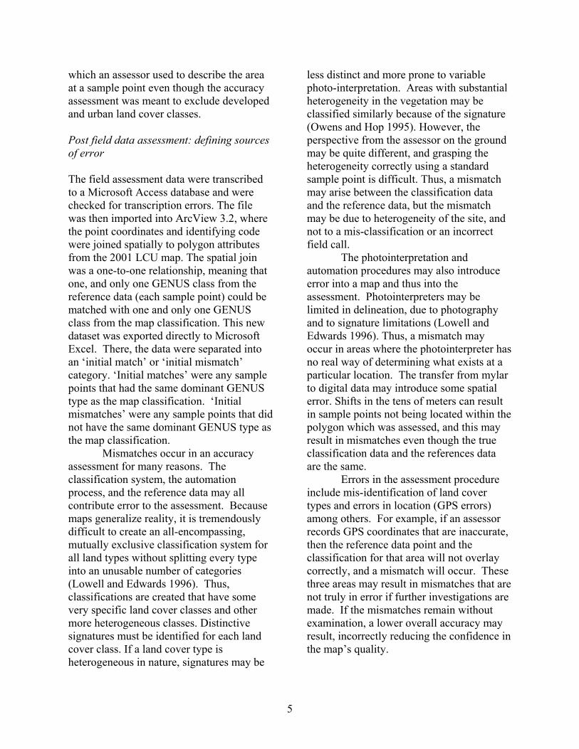
occurrence of the 243 initial mismatches (Table 2). Sometimes two or more factors explained the reason for a mismatch. In these instances, the principle error justification is used to display the data. The largest category resulting in initial mismatches is the ‘inclusion’ category (22% of the initial mismatches). This category explains a difference in scale between what the assessor sees and what the photointerpreter considers large enough to draw. Figure 2 illustrates an example of

Table 2. Error types developed after examining initially mismatched sample points.

JUSTIFICATION DESCRIPTION ERROR TYPE NUMBER POINTS

Both calls wrong The field call and map classification are both incorrect mismatch 4

Changed field call based on datasheet assessment

Sufficient information on datasheet exists to alter field call

mismatch justified correct

4 46

Classification Assessor is unfamiliar with landcover classification and lacks key

mismatch justified correct

3 1

Density issue Difference on ground and from air of the density or cover of a species

mismatch justified correct

4 1

GPS error GPS receiver put assessor in the wrong location

mismatch justified correct

3 8

Height Tree height appears different to assessor and photo-interpreter mismatch 1

Inclusion The assessor's call is below Minimum Mapping Unit (MMU) justified correct 54

PI call The photo-interpreter mis-classified a vegetation type mismatch 28

Point versus polygon Assessor's field call does not reflect the heterogeneity of the entire region mismatch 3

Signature limitations Nature of the photographs limits photo-interpreters ability to see certain signatures

mismatch 4

Spatial error in automation Differences > 20m between the vector coverage and the DOQ

mismatch justified correct

2 45

Time factor Assessment made at different time from photointerpretation of the area

mismatch justified correct

14 2

Transition zone Assessment made in an area near boundary of polygon; ecotone

mismatch justified correct 8

1 Too little information insufficient information to keep the point DROP 5

TOTAL NUMBER OF POINTS INITIALLY IDENTIFIED AS MISMATCHED 243

9

Figure 2. Sparganium inclusion. The scale is approximately 1:2,300.

example of a sample point that the assessor identified as Sparganium- dominant. The True Color aerial photograph was taken in July 2001. The assessment group examined the area and noted the dark, almost black patch of Sparganium (Sp) that is present in two different polygons. Although the assessment team could see the patch the assessor was seeing, the photointerpreter did not consider the Sparganium patch as large enough to delineate on its own. Since the field identification was accepted as valid, with ‘inclusion’ as the error type, the reference data (the assessor’s dataset) for this point was updated with the classification for the polygon in which it existed.

The next largest source of error is when a field call is ‘changed’ by the assessment team to match the data provided on the field datasheet. This source of mismatching accounted for 20.6% of the total mismatches. For example, sample point 388 was identified by the assessor as Sparganium-dominant. The map classification in 2001 for that area is Mixed Emergent. The general vegetation characteristics described on the assessor’s datasheet are “… Could also be Sparganium

Marsh; there is a mix of Sp and Ty (Typha) and Leersia, with some Ph, pretty well mixed; also with a Sc patch or two. It is hard to differentiate which is dominant”. The documentation of more than one type of vegetation potentially dominant, a mixture of emergent species, and a digital photograph taken at the sample point helped the assessment group to change the reference data at the sample point to Mixed Emergents.

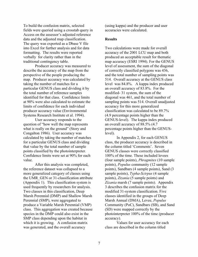
Another substantial source of mismatches was spatial error due to digital automation of the classified dataset (19.3% of the total initial mismatches). Across the entire coverage, evidence showed that spatial variation existed between the vector coverage and the DOQQ (Figure 3). The assessor made a correct reference call of Submerged Vegetation based upon the datasheet information and the water depth readings taken. However, the overlay analysis located a Submerged Vegetation sample point on a Floodplain Forest polygon. Using the measuring tool in ArcView, the assessment team learned that

$

ZiM

Ny-Zi

Sp

approx. 50 m

$

$

$

$

$

SV

Sg

FF

'SV'

Figure 3. Spatial shift in automation. The scale is approximately 1:2,000.

10

spatial shift in this region of the map ranged from ten to thirty meters. A visual correction was made to the location of the classified polygons, which moved the sample point over the region of the Submerged Vegetation. The reference data sample point was adjusted as correct. Mismatches that were identified as mistakes in classification were varied in their types (11.5% of the initial mismatches). These included differences in perspective regarding the classification of agriculture areas, the density of vegetation in certain areas, and the height of vegetation. The majority of these mismatches remained errors after analysis because the producer and assessor’s scales of reference are vastly different.

Misidentification of a signature, decisions of where to put a boundary line, and signature limitations on the photographs accounted for about 13% of the initial mismatches. Figure 2 also illustrates this variability due to photointerpretation. Since the dark signature of Sparganium was not classified as its own polygon, the photointerpreter could draw the boundary of the polygon outside the dark patch and add it to the area classified as a Zizania marsh. However, the Sparganium patch was divided between two polygons, and the other half was classified as Ny-Zi.

GPS error accounted for about three percent of the initial mismatches. GPS errors were due to assessing the vegetation at a distance from the actual sample point coordinates, mis-reading the GPS unit, or transcribing the coordinates incorrectly. In one example, a point had to be taken on a levee twenty meters south of the actual vegetation to be sampled because no boat access was available. The overlay analysis assigned a map classification of ‘Levee’ at this sample point against the reference data of Nelumbo, producing an initial mismatch. However, the reference data call, Nelumbo,

was correct when checked by the assessment group because the correct polygon was assessed.

Time factors contribute to 6.5% of the initial mismatches. The 2001 aerial photographs were flown in August 2001, and the assessments did not commence until the end of September. In more than one instance, areas that were classified as Mudflats in August had grown sufficient annual vegetation in the fall to be assessed as ‘Echinochloa’. On several occasions, senescing plants and rising water levels in October produced regions that were assessed as Open Water or as Submerged Vegetation where previously emergent vegetation had grown.

Transition zones accounted for three percent of the initial mismatches. Transition zones are areas where sample points fall within five meters of two polygons. At times, when the vegetation was assessed, it would include both polygon classes. Insufficient information was recorded on the field data sheet to determine into which polygon the assessor was focusing.

Other justification types each account for less than three percent of the initial mismatches. These types include the reference data and the classification being incorrect, issues of density cover for certain species, the height of trees, the scale of perception (point versus polygon), signature limitations, and too little information.

Fourteen points of the 171 initial matches that were overlaid on a photo-mosaic appeared to fall close to a boundary line. The visible spatial error (due to automation) with the mismatched sample points did not affect any of these matched points. This confirmation was determined by adjusting the boundary lines temporarily to match the mosaic or the DOQQ and observe where the point existed. All 272 points remained as matches for the final dataset.

11

At the end of this examination, 160 of the initially mismatched points were adjusted as correct and were added to the 272 initially matched points, 77 points remained as errors, and five points were dropped for a total of 514 points. The most substantial sources for error in the remaining mismatched points were: photo-interpretation call (36%), time factor (18%), and transition zones (10%). Discussion The values calculated for overall accuracy, 83% for the GENUS level classification and 88% for the modified 31-classification system, are acceptable according to the standard of 80% set by the National Park Service (Environmental Systems Research Institute et al. 1994). The assessors anticipated that overall accuracy, as well as producer and user accuracies, would increase as the classes became more generalized. This prediction was confirmed for overall accuracy by an increase of five percentage points. The proportion of values for producer accuracy below the 80% standard decreased from the GENUS level 13/37 = 0.35) to the modified 31-classification level (4/18 = 0.22). The proportion of values for user accuracy below the 80% standard decreased from the GENUS class level (11/31 = 0.35) to the modified 31-classification level (1/17 = 0.06).

The overall accuracy represents the degree of accuracy across all classes on the map, but it does not explain where discrepancies exist (Story and Congalton, 1991). The error matrix allows both the map producer and the user to know more about where errors exist in the map. Examining an error matrix can be confusing at first. Several key concepts need to be kept in mind when interpreting this type of table. One important concept to remember

is that two different values, producer and user accuracies, are derived from the same table. Producer accuracy describes the errors of omission, that is, the errors made by the map producer in classifying some areas as other than what the assessor found in the field. User accuracy describes errors of commission on the part of the producer, because all areas that are misclassified have been put into another class.

An example of errors of omission and commission can be found by looking at the producer and user accuracies for the GENUS class Lythrum. Three areas that the assessor observed to be dominated by Lythrum were correctly classified by the map producer as Lythrum. However, the assessor found two additional areas also dominated by Lythrum that the producer ‘omitted’ by classifying these areas as Wet Meadow Shrubs. Examining user accuracy shows four total areas classified as Lythrum. In this case, the assessor observed that three of these areas were Lythrum-dominant, however, a fourth area was dominated by Mixed Emergents. The error of commission occurs because the producer classified an area as Lythrum dominant when the area was assessed to be otherwise. These errors of omission and commission are anticipated to some extent, since Lythrum is a tall, shrub-like perennial herb and might be ‘confused’ with a photo signature for wet meadow shrubs, or, in higher water areas, for mixed emergent vegetation, either of which Lythrum could be a constituent. In this example, the difference in producer and user accuracies is significant. From the perspective of the map producer, the final producer accuracy of 60% means that the photointerpreter is only mapping this GENUS class three-fifths of the time correctly, but it also shows that the misclassification into another GENUS class, wet meadow shrub, is a reasonable error. From the user perspective, a visit to a site

12

labeled on the map as Lythrum would mean the person would be in a Lythrum-dominant site 75% of the time. But 25% of the time, the user would be somewhere else (likely in a bed of mixed emergent vegetation that might include Lythrum). These errors of omission and commission are crucial for the reader of a map to understand if the types of errors are logical and can be accommodated.

One additional note about the tables is important to remember. The map producer and the user need to know that the larger the sample size for each class, the smaller the confidence limit and the greater the ‘confidence’ that the true value for the population exists between the two confidence limits. The inverse is true for small sample sizes. Since the number of sample points for each GENUS class was determined by the number of classified polygons for each GENUS class, the results for rare classes like Lythrum appear to display greater discrepancies than do larger classes.

Several important conclusions can be drawn from examining the error matrices. At the GENUS level, four classes were correctly classified 100% of the time. Phragmites and Populus communities are perennial and are mostly static vegetation types, but Zizania and Zizania marsh are comprised of annual species that are neither common nor static. The high accuracy attributed to all four GENUS classes is due to unique signatures, which even in low densities and with infrequent presence from one year to the next, can be detected by the photointerpreter.

GENUS classes dominated by woody vegetation often had the highest producer accuracies (floodplain forests at 98%, Salix and Populus communities at 98% and 100%, respectively). These areas are the most static of all areas of the river and are not likely to be altered by anything but severe flooding or by human activities (e.g.,

logging). Because of the highly generalized nature of the categories and the simple distinctions between different forest types, field assessment is much easier to confirm on the aerial photographs. In these examples, the error of omission is low, i.e, few areas identified as floodplain forests were something other than floodplain forests. A notable exception to the high forest producer accuracy is the lowland forest class, in which three of the areas identified by the assessor as lowland forest were mapped as floodplain forest. The constituents of these areas contain tree types (Pinus sp., Quercus sp.) that are considered to be less flood-tolerant and were visible to the assessment team during the data assessment in the field.

Conversely, for the shrub-scrub category, which is an upland vegetation category of mixed shrubby and herbaceous vegetation, the producer accuracy was 0% for both assessments. The producer accuracy shows that 75% of the sample points identified as shrub-scrub on the ground were incorrectly classed by the photointerpreter as wet-meadow shrubs. The remaining 25% of the shrub-scrub sampling points were mis-classified as Salix communities. The error of omission for this class is 100%, because the areas that should have been classified as shrub-scrub were omitted from that category.

Aquatic vegetation classes were often mismatched into a variety of other classes. For example, sampling points identified on the ground as Nymphaea-dominated were variously classified by the photointerpreter as Nymphaea (70%), Nelumbo-dominated (10%), a mix of rooted-floating aquatics (5%), a sandbar (5%), Sparganium-dominated(5%), or as an area dominated by submerged vegetation (5%) (Appendix 2). In nearly every case, the assessment team could find Nymphaea signatures in the area of the sampling point, but they gave

13

explanations at each location for why Nymphaea was not the dominant species for that particular area. The final producer accuracy was 71%; but it was clear that except for the sandbar category all of the other types were reasonable community types in which Nymphaea might exist or be ‘confused’. Errors of commission are illustrated in user accuracy for Phalaris (90% accuracy; Appendix 2). Areas labeled as Phalaris-dominated by the photointerpreter had a 90% probability of actually being Phalaris-dominated when a person visited the site, but a 10% probability of being something else. The types of ‘confusion’ in that 10% margin include: an agriculture area (2%), an area mixed with grasses and forbs (2%), a Leersia bed (2%), a bed of mixed emergents (3%), or an area dominated by sedges (2%). The user may decide that these areas are not sufficiently different in terms of habitat to be of much consequence. On the other hand, someone using the map to document the spread of Phalaris would need to be aware that 10% of the sites that they visit may be dominated by species other than Phalaris.

The producer and the user accuracies for the modified 31- classification display similar results, but there are some important differences (Appendix 3). Three of the classes (Populus Community, Sand Bars, and Sand) do not change from the GENUS-level classes in terms of being classified correctly 100% of the time. Deep Marsh Annuals (DMA) contain the Zizania and Zizania marsh classes. Collapsing these categories did not change the producer accuracy, but the increased sample size of 12 decreased the width of the confidence limits by three to six percentage points, increasing the confidence of the actual value of the producer accuracy. A generalized class group that ‘benefits’ from the collapsing of GENUS-

classes is Rooted-Floating Aquatics (RFA; Appendix 3). Individually, two of the three constituents had producer accuracy falling below the 80% level standard (Appendix 2). The Nymphaea-dominated GENUS class has a producer accuracy of 71% (20 samples), Rooted-Floating Aquatics are 60% (5 samples), and Nelumbo-dominated areas are 92% (36 samples). After collapsing these three categories, the producer accuracy is 92% (60 samples), and the confidence limits are narrowed to increase the confidence in the value (a decrease of two to twenty-five percentage points). In terms of user accuracies, some interesting trends are displayed (Appendix 3). The Deep Marsh Annuals (DMA) class is reported to have a user accuracy of 86%, with confusion into Variable Marsh Perennials (14%). What this likely means is that areas labeled as DMA have perennial emergent species dominating in at least 14% of the areas assessed. Rooted-Floating Aquatics (RFA) have a 93% user accuracy, meaning that a person standing in an area labeled as RFA by the photointerpreter is likely standing in Nymphaea, Nelumbo, or some mixture of the two with other species. The errors of commission total 8% and include the possibility that the observer is actually standing in an area dominated by variable marsh perennials rather than in rooted floating aquatics (three percent). Since marshes may have rooted floating aquatic species as primary components of the vegetation, this ‘confusion’ is reasonable. In addition, the assessor observed open water two percent of the time and identified the area as dominated by submerged vegetation three percent of the time. Errors for initial and final mismatched points can be divided into two groups: errors which are correctable and errors which cannot be corrected. Many of the errors made by the assessor in the field

14

portion of the study are correctable. At the same time, these errors demonstrate the danger in assuming that the ground data or reference data are true without a thorough examination of all data available. In many assessments, reference data are considered as ‘truth’. Some of the errors due to time of year and photointerpreter’s calls can be corrected as well. However, these types of errors demonstrate, along with errors of transition and perspective, some of the variation inherent in all maps and in the assessment process.

The inclusions error type may have been reduced if the appropriate plot size had been used. Although the minimum mapping unit was approximately one-half hectare (approximately 70 X 70 meters) the visualized field plots were smaller due to a mistake in determining the plot size. Thus, the assessor only considered an area that was three-quarters the size of the minimum mapping unit. This may have affected the reference dataset, particularly in areas where the vegetation was considerably taller than the observer.

The assessor was unfamiliar with the LCU classification system and lacked a descriptive key to the GENUS classes. Because sufficient detail was recorded in the datasheets, the accuracy assessment team was able to change the field call to match the information that was provided on the datasheet. This adjustment usually resulted in an agreement with the photo-interpreted map call. However, since recording of the percent-cover was not required, even the adjusted information was based primarily upon judgment rather than just on the exclusive quantitative examination of the datasheet information. This error justification was applied to observations of both the individual assessor and the team of assessors.

Another issue that is more difficult to correct after map production is the spatial

error. Offsets across the entire study area ranged from 0 meters to almost 50 meters in some cases. The GIS staff narrowed the spatial error source to a scanning problem and has taken steps to eliminate this type of error in the future. Some of the overlays scanned had insufficient leaders which resulted in some data being stretched before the scanner had time to initialize (Larry Robinson, 2002, personal communication). This resulted in the ‘stretched’ areas having higher than expected spatial error. National Map Accuracy Standards state that for 1:12,000 DOQQs, the base maps used to create the LCU, 90% of all well-defined points will be ten meters or less from their ‘true’ location on the earth’s surface. Spatial offsets of 20-30 meters indicated a problem somewhere in the LCU production process. Once the large format scanner was identified as the problem, all subsequent scans used an 11 X 17 flatbed and the 9 X 9 interpreted transparent aerial photograph. During the data assessment, the team found that the majority of points that fell into an area of considerable spatial shift could be adjusted correct once the polygons were shifted to align with the DOQQs. This shifting resulted in many mismatched points now overlaying the correct polygon. This adjustment is a time-consuming process and one that will be greatly reduced if spatial error is identified before the final digital map is completed.

On several occasions, the photointerpreter mis-classified the dominant vegetation type existing in a particular area; the assessment at this point successfully identified areas in which the photointerpreter could work on signature identification. Some of these types of errors may be correctable through increased familiarity with signatures of specific classes. Some of these variations, however, are inherent in the photo-interpretive process (Congalton 1991; Lowell and Edwards

15

1996), and any user of a map needs to anticipate this and not assume that these variations are an automatic indication of poor map quality.

Another type of potential error inherent in LCU maps is the photointerpreter’s choice of where to draw the line. Figure 2 illustrates where the photointerpreter drew a line through the Sparganium. Most of the Sparganium exists as an inclusion in a bed of Nymphaea. The sample point was justified correct after examination, primarily because the vegetation itself was slightly smaller than MMU. However, the assessment team also thought that if the line had been extended farther around the Sparganium, it could have been better placed within the larger Zizania marsh polygon. Again, the user needs to understand that photo-interpretation, which can be quite subjective at times, requires the map producer to make a decision where to put a line even though no corresponding demarcation may exist on the ground.

GPS error appears to be nearly impossible to avoid in thematic accuracy assessments. If GPS error is large enough, the error will need to be corrected either by using better euipment or by averaging many points at each sample site. GPS error in this study is identified as readings that display a point into a polygon other than the one that was intended for assessment, and the boundary between polygons is typically within five meters of the point. Less than 5% of all initial mismatches are attributed to GPS error. Many of the coordinates in early fall were collected over water and in non-forested herbaceous areas. Nearly all of the terrestrial points were sampled after leaf fall (late October). These sampling times may have helped to reduce the multi-path error associated with collecting points in heavily forested areas prior to leaf off.

Another type of error that may be unavoidable occurs when the time of year

the photographs are taken differs from when the assessment is performed (Congalton 1991. Two significant disturbances occurred in Pool 8 between 2000 and 2001, and the vegetation in some areas varied dramatically from one year to the next. A prolonged flood from April to June 2001 (the third highest on record) followed by a planned drawdown of the pool, changed hydrology and habitat for an entire growing season. Some of the changes observed in vegetation types are entirely due to these ecological perturbations. An example of this change is illustrated by the substantial increase of Zizania, which requires inundation early in its growth cycle, between 2000 and 2001.

If at all possible, vegetation types subject to early senescence need to be assessed close to their peak biomass. Due to the timing of the study, this was not possible. During this assessment, the rooted floating aquatics, including Nelumbo and Nymphaea, and some of the emergents, especially Sagittaria, begin to senesce, which affected sampling. Other species, particularly more persistent plants including Typha, Phalaris, and the terrestrial woody species, were not impacted at all. Differences in perspective between what the photointerpreter can see on the photo and what the assessor can see on the ground are an inevitable part of an accuracy assessment. The photointerpreter can ‘see’ large patterns of vegetation in less detail while the assessor can see less distance in greater detail. The error matrices help describe some of these errors in perspective, and in most cases, the user will be able to understand these differences if the classification system is logical. From this study, the assessment team has concluded that the 2001 LCU map for Pool 8 of the Mississippi River has an acceptable overall accuracy and that the errors in producer and user accuracies are reasonable. The team also has a blueprint

16

for future accuracy assessments, which are outlined in Appendix 4. With a thorough review of the initial mismatched points, the assessment team has a better understanding of overall accuracy of the 2001 map. Developing an error source table and applying it to the sample points revealed numerous false errors that could be adjusted. Since many initial mismatches were generated by the reference data, the assumption that reference data are ‘truth’ was violated. The post-field assessment rectified the errors; however, cost in time and resources increased. A practical cost-benefit analysis is essential before an accuracy assessment is implemented; depending upon the needs of the user, an entire map does not always need to be assessed for thematic accuracy. Different areas might be given higher priority, especially if resources and time are limited (Stehman and Czaplewski 1998). If the accuracy assessment can find ‘true’ errors that improve map production and which are understandable to the user, then future assessments of the same area may not necessarily have to cover as broad a scope. Acknowledgements I thank Sara Lubinski, Jennifer Dieck, and Larry Robinson for coordinating the project and for being members of my committee. I thank Linda Leake and UMESC for funding this project; and I thank Jennifer Sauer, Pete Boma, Erin Hoy, and Jeff Yanke who participated in field data collection. For mentoring and perspectives on accuracy assessment, I thank Kevin Hop (USGS). I thank also Dr. David McConville, Barry Drazkdowski, Tracy Trople, and Martha Roldan of St. Mary’s University for reviewing the paper. Finally, I thank my husband, Paul, for his assistance designing

macros and the crosstab query and for his love. Literature Cited Congalton, R.G. (1991). A review of

assessing the accuracy of classifications of remotely sensed data. Remote Sensing Environment 37:35-46.

Environmental Systems Research Institute, National Center for Geographic Analysis, and The Nature Conservancy (1994). Accuracy assessment procedures: NBS/NPS vegetation mapping program. Final draft. Prepared for: United States Department of the Interior- National Biological Survey and National Park Service. November 1994.

Lowell, K.E. and G. Edwards (1996). Modelling heterogeneity and change in natural forests. Geomatica 50(IV): 425-440.

Moissen, G. C., D.R. Cutler, and T.C. Edwards (2000). Generalized linear mixed models for analyzing error in a satellite-based vegetation map in Utah. In: Quantifying spatial uncertainty in natural resources: Theory and applications for GIS and remote sensing. Edited by T. Mower and R.G. Congalton; Ann Arbor Press, Chelsea, MI.

Owens, T. and K. Hop (1995). LTRMP Standard Operating Procedures: Photointerpretation. Program Report 95-P008-1; July 1995.

Stehman, S.V. and R.L. Czaplewski (1998). Design and analysis for thematic map accuracy assessment: fundamental principles. Remote Sensing Environment 64:331-344.

Story, M. and R. G. Congalton (1986). Accuracy assessment: a user perspective. Photogrammetric Engineering and Remote Sensing 52 (III): 397-399.

17

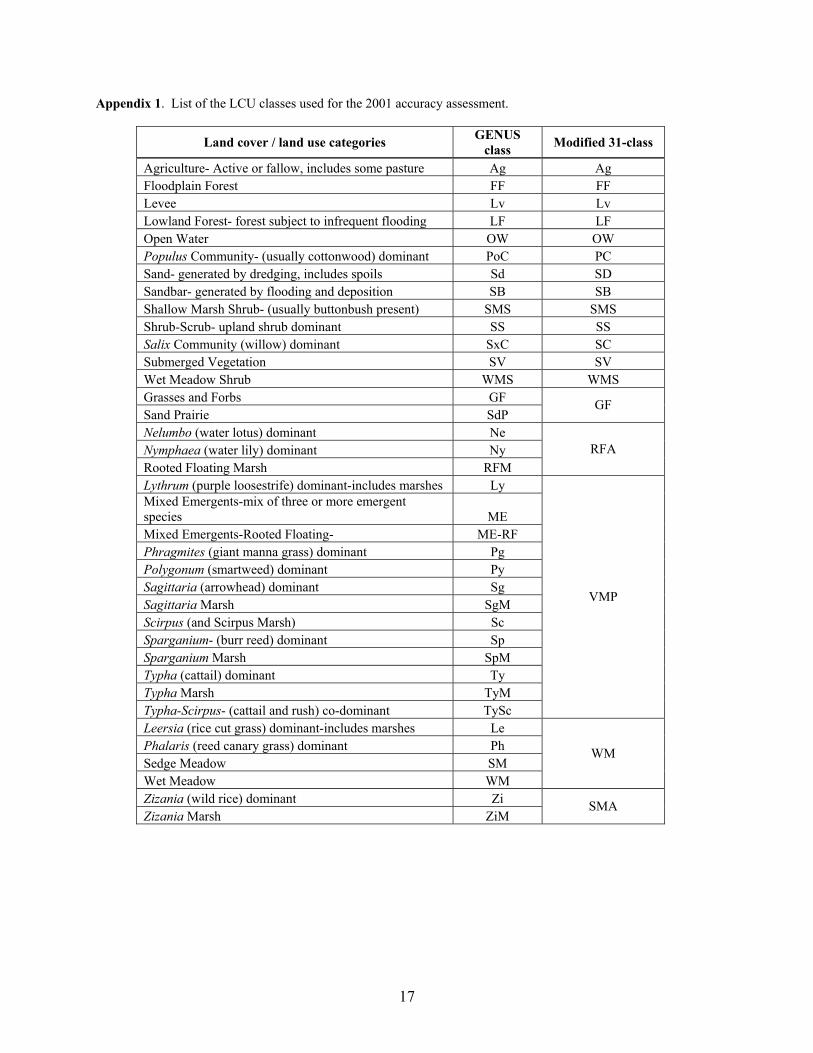
Appendix 1. List of the LCU classes used for the 2001 accuracy assessment.

Land cover / land use categories GENUS class Modified 31-class

Agriculture- Active or fallow, includes some pasture Ag Ag Floodplain Forest FF FF Levee Lv Lv Lowland Forest- forest subject to infrequent flooding LF LF Open Water OW OW Populus Community- (usually cottonwood) dominant PoC PC Sand- generated by dredging, includes spoils Sd SD Sandbar- generated by flooding and deposition SB SB Shallow Marsh Shrub- (usually buttonbush present) SMS SMS Shrub-Scrub- upland shrub dominant SS SS Salix Community (willow) dominant SxC SC Submerged Vegetation SV SV Wet Meadow Shrub WMS WMS Grasses and Forbs GF Sand Prairie SdP

GF

Nelumbo (water lotus) dominant Ne Nymphaea (water lily) dominant Ny Rooted Floating Marsh RFM

RFA

Lythrum (purple loosestrife) dominant-includes marshes Ly Mixed Emergents-mix of three or more emergent species ME Mixed Emergents-Rooted Floating- ME-RF Phragmites (giant manna grass) dominant Pg Polygonum (smartweed) dominant Py Sagittaria (arrowhead) dominant Sg Sagittaria Marsh SgM Scirpus (and Scirpus Marsh) Sc Sparganium- (burr reed) dominant Sp Sparganium Marsh SpM Typha (cattail) dominant Ty Typha Marsh TyM Typha-Scirpus- (cattail and rush) co-dominant TySc

VMP

Leersia (rice cut grass) dominant-includes marshes Le Phalaris (reed canary grass) dominant Ph Sedge Meadow SM Wet Meadow WM

WM

Zizania (wild rice) dominant Zi Zizania Marsh ZiM

SMA

18

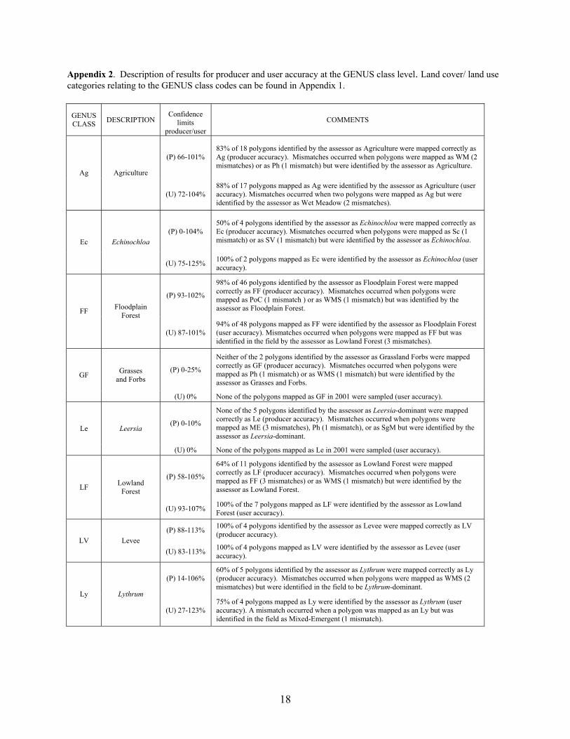
Appendix 2. Description of results for producer and user accuracy at the GENUS class level. Land cover/ land use categories relating to the GENUS class codes can be found in Appendix 1.

GENUS CLASS DESCRIPTION

Confidence limits

producer/user COMMENTS

(P) 66-101% 83% of 18 polygons identified by the assessor as Agriculture were mapped correctly as Ag (producer accuracy). Mismatches occurred when polygons were mapped as WM (2 mismatches) or as Ph (1 mismatch) but were identified by the assessor as Agriculture.

Ag Agriculture

(U) 72-104% 88% of 17 polygons mapped as Ag were identified by the assessor as Agriculture (user accuracy). Mismatches occurred when two polygons were mapped as Ag but were identified by the assessor as Wet Meadow (2 mismatches).

(P) 0-104% 50% of 4 polygons identified by the assessor as Echinochloa were mapped correctly as Ec (producer accuracy). Mismatches occurred when polygons were mapped as Sc (1 mismatch) or as SV (1 mismatch) but were identified by the assessor as Echinochloa. Ec Echinochloa

(U) 75-125% 100% of 2 polygons mapped as Ec were identified by the assessor as Echinochloa (user accuracy).

(P) 93-102%

98% of 46 polygons identified by the assessor as Floodplain Forest were mapped correctly as FF (producer accuracy). Mismatches occurred when polygons were mapped as PoC (1 mismatch ) or as WMS (1 mismatch) but was identified by the assessor as Floodplain Forest. FF Floodplain

Forest

(U) 87-101% 94% of 48 polygons mapped as FF were identified by the assessor as Floodplain Forest (user accuracy). Mismatches occurred when polygons were mapped as FF but was identified in the field by the assessor as Lowland Forest (3 mismatches).

(P) 0-25%

Neither of the 2 polygons identified by the assessor as Grassland Forbs were mapped correctly as GF (producer accuracy). Mismatches occurred when polygons were mapped as Ph (1 mismatch) or as WMS (1 mismatch) but were identified by the assessor as Grasses and Forbs.

GF Grasses and Forbs

(U) 0% None of the polygons mapped as GF in 2001 were sampled (user accuracy).

(P) 0-10%

None of the 5 polygons identified by the assessor as Leersia-dominant were mapped correctly as Le (producer accuracy). Mismatches occurred when polygons were mapped as ME (3 mismatches), Ph (1 mismatch), or as SgM but were identified by the assessor as Leersia-dominant.

Le Leersia

(U) 0% None of the polygons mapped as Le in 2001 were sampled (user accuracy).

(P) 58-105%

64% of 11 polygons identified by the assessor as Lowland Forest were mapped correctly as LF (producer accuracy). Mismatches occurred when polygons were mapped as FF (3 mismatches) or as WMS (1 mismatch) but were identified by the assessor as Lowland Forest. LF Lowland

Forest

(U) 93-107% 100% of the 7 polygons mapped as LF were identified by the assessor as Lowland Forest (user accuracy).

(P) 88-113% 100% of 4 polygons identified by the assessor as Levee were mapped correctly as LV (producer accuracy).

LV Levee (U) 83-113% 100% of 4 polygons mapped as LV were identified by the assessor as Levee (user

accuracy).

(P) 14-106% 60% of 5 polygons identified by the assessor as Lythrum were mapped correctly as Ly (producer accuracy). Mismatches occurred when polygons were mapped as WMS (2 mismatches) but were identified in the field to be Lythrum-dominant.

Ly Lythrum

(U) 27-123% 75% of 4 polygons mapped as Ly were identified by the assessor as Lythrum (user accuracy). A mismatch occurred when a polygon was mapped as an Ly but was identified in the field as Mixed-Emergent (1 mismatch).

19

Appendix 2 (cont’d). Description of results for producer and user accuracy at the GENUS class level.

GENUS CLASS DESCRIPTION

Confidence limits

producer/user COMMENTS

(P) 35-92% 64% of 11 polygons identified by the assessor as Mixed Emergents were mapped correctly as ME (producer accuracy). Mismatches occurred when polygons were mapped as Ly (1 mismatch), Ph (2 mismatches), or as Sp (1 mismatch) but were identified by the assessor as Mixed Emergent. ME Mixed

Emergents

(U) 41-99% 70% of 10 polygons mapped as ME were identified by the assessor as Mixed Emergents (user accuracy). Mismatches occurred when polygons were mapped as ME but were identified in the field as Leersia-dominant (3 mismatches).

(P) 0-50%

The single polygon identified by the assessor as Mixed Emergent-Rooted Floating was not mapped correctly as ME-RF (producer accuracy). The mismatch occurred when a polygon was mapped as SpM but was identified in the field as Mixed Emergent-Rooted Floating (1 mismatch) .

ME-RF

Mixed Emergent-

Rooted Floating Aquatics (U) 0% None of the polygons mapped as ME-RF in 2001 were sampled (user accuracy).

(P) 83-101% 92% of 36 polygons identified by the assessor as Nelumbo-dominant were mapped correctly as Ne (producer accuracy). Mismatches occurred when polygons were mapped as Sg but were identified in the field as Nelumbo-dominant (3 mismatches).

Ne Nelumbo

(U) 77-97%

87% of 38 polygons mapped as Ne were identified by the assessor as Nelumbo (user accuracy). Mismatches occurred when polygons were mapped as Ne but were identified in the field as Open Water (1 mismatch), Nymphaea-dominant ( 2 mismatches), Rooted Floating (1 mismatch), or Sagittaria-dominant (1 mismatch).

(P) 53-90%

71% of 21 polygons identified by the assessor as Nymphaea were mapped correctly as Ny (producer accuracy). Mismatches occurred when polygons were mapped as Ne (2 mismatches), RF (1 mismatch), Ne (1 mismatch), Sb (1 mismatch), Sp (1 mismatch), or as SV (1 mismatch) but were identified in the field as Nymphaea-dominant.

Ny Nymphaea

(U) 72-104%

88% of 17 polygons mapped as Ny were identified by the assessor to be Nymphaea (user accuracy). Mismatches occurred when polygons were mapped as Ny but were identified in the field as Sagittaria (1 mismatch) and Submerged Vegetation (1 mismatch).

(P) 74-97%

85% of 34 polygons identified by the assessor as Open Water were mapped correctly as OW (producer accuracy). Mismatches occurred when polygons were mapped as Ne (1 mismatch), Sg (1 mismatch), and SV (3 mismatches) but were identified in the field as Open Water. OW Open water

(U) 98-102% 100% of 29 polygons mapped as OW were identified by the assessor to be Open Water (user accuracy).

(P) 95-105% 100% of 10 polygons identified by the assessor as Phragmites were mapped correctly as Pg (producer accuracy).

Pg Phragmites (U) 95-105% 100% of 10 polygons mapped as Pg were identfied by the assessor to be Phragmites

(user accuracy).

(P) 81-96%

88% of 60 polygons identified by the assessor as Phalaris-dominant were mapped correctly as Ph (producer accuracy). Mismatches occurred when polygons were mapped as Sg (4 mismatches), WMS (2 mismatches) or as Sc (1 mismatch) but were identified in the field as Phalaris.

Ph Phalaris

(U) 84-98%

91% of 58 polygons mapped as Ph were identified by the assessor to be Phalaris-dominant (user accuracy). Mismatches occurred when polygons were mapped as Ph but were identified in the field as Agriculture (1 mismatch), Grassland Forbs (1 mismatch), Leersia (1 mismatch), or as Mixed Emergent (2 mismatches).

20

Appendix 2 (cont’d). Description of results for producer and user accuracy at the GENUS class level.

GENUS CLASS DESCRIPTION

Confidence limits

producer/user COMMENTS

(P) 96-104% 100% of 12 polygons identified by the assessor as Populus-dominated communities were mapped correctly as PoC (producer accuracy).

PoC Populus community

(U) 76-108% 92% of 13 polygons mapped as PoC were identified by the assessor to be Populus-dominated communities (user accuracy). A mismatch occurred when a polygon was mapped as PoC but was identified in the field as Floodplain Forest (1 mismatch).

(P) 0-25% Neither of the 2 polygons identified by the assessor as Polygonum-dominated were mapped correctly as Py (producer accuracy). Mismatches occurred when polygons were mapped as Sc but were identified in the field as Polygonum (2 mismatches).

Py Polygonum

(U) 0% The single polygon mapped as Py was not identified by the assessor to be Polygonum-dominant (user accuracy). The mismatch occurred when an area was mapped as Py but was identified in the field to be Sagittaria-dominant (1 mismatch).

(P) 14-106% 60% of 5 polygons identified by the assessor as Rooted Floating were mapped correctly as RF (producer accuracy). Mismatches occurred when polygons were mapped as Ne (1 mismatch) and SV (1 mismatch) but were identified in the field as Rooted Floating.

RF Rooted Floating (aquatics)

(U) 27-123% 75% of 4 polygons mapped as RF were identified by the assessor as Rooted Floating (user accuracy). A mismatch occurred when a polygon was mapped as RF but was identified in the field as Nymphaea-dominant (1 mismatch).

(P) 88-113% 100% of 4 polygons identified by the assessor in the field as Sandbars were mapped correctly as SB (producer accuracy).

SB Sandbar (U) 41-119%

80% of 5 polygons mapped as SB were identified by the assessor in the field as Sandbar (user accuracy). A mismatch occurred when a polygon was mapped as SB but was identified in the field as Nymphaea-dominant (1 mismatch).

(P) 86-102%

94% of 35 polygons identified by the assessor in the field as Scirpus-dominated were mapped correctly as Sc (producer accuracy). Mismatches occurred when polygons were mapped as Sg (1 mismatch) or as Zi ( 1 mismatch) but were identified in the field as Scirpus-dominant.

Sc Scirpus

(U) 67-90% 79% of 35 polygons mapped as Sc were identified in the field by the assessor as Scirpus-dominant (user accuracy). Mismatches occurred when polygons were mapped as Sc but were identified in the field as Echinochloa (1 mismatch), Phalaris (1 mismatch), Polygonum (2 mismatches), Sparganium (2 mismatches), Salix Community (1 mismatch), and Wet Meadow (2 mismatches).

(P) 83-117% 100 % of 3 polygons identified by the assessor in the field as Sand were mapped correctly as SD (producer accuracy).

SD Sand (U) 27-123%

75% of 4 polygons mapped as SD were identified in the field by the assessor as Sand (user accuracy). A mismatch occurred when a polygon was mapped as SD but was identified in the field to be a Sand Prairie (1 mismatch).

(P) 57-115% 86% of 7 polygons identified by the assessor as Sand Prairie were mapped correctly as SdP (producer accuracy). A mismatch occurred when a polygon was mapped as SD (1 mismatch) but was identified in the field as Sand Prairie. SdP Sand Prairie

(U) 92-108% 100% of 6 polgyons mapped as SdP were identified by the assessor in the field as Sand Prairie (user accuracy).

21

Appendix 2 (cont’d). Description of results for producer and user accuracy at the GENUS class level.

GENUS CLASS DESCRIPTION

Confidence limits

producer/user COMMENTS

(P) 69-101%

85% of 20 polygons identified by the assessor in the field as Sagittaria were mapped correctly as Sg (producer accuracy). Mismatches occurred when polygons were mapped as Ne (1 mismatch), Ny (1 mismatch), or Py (1 mismatch) but were identified in the field to be Sagittaria-dominant.

Sg Sagittaria

(U) 42-75%

59% of 29 polygons mapped as Sg were identified by the assessor in the field as Sagittaria-dominated (user accuracy). Mismatches occurred when areas were mapped as Sg but were identified in the field as Nelumbo (3 mismatches), Open Water (1 mismatch), Phalaris (4 mismatches), Scirpus (1 mismatch), Sagittaria Marsh (2 mismatches), or Wet Meadow (1 mismatch).

(P) 0-104%

50% of 4 polygons identified by the assessor in the field as Sagittaria marsh were mapped correctly as SgM (producer accuracy). Mismatches occurred when polygons were mapped as Sg (2 mismatches) but were identified in the field to be Sagittaria Marsh. SgM Sagittaria

Marsh

(U) 5-128% 67% of 3 polygons mapped as SgM were identified by the assessor in the field as Sagittaria Marsh (user accuracy). A mismatch occurred when a polygon was mapped as SgM but was identified in the field as Leersia-dominant (1 mismatch).

(P) 73-101%

87% of 23 polygons identified by the assessor in the field as Sparganium- dominated were mapped correctly as Sp (producer accuracy). Mismatches occurred when polygons were mapped as Sc (2 mismatches) and ZiM (1 mismatch) but were identified in the field to be Sparganium-dominant.

Sp Sparganium

(U) 73-101%

87% of 23 polygons mapped as Sp were identified by the assessor in the field as Sparganium-dominated (user accuracy). Mismatches occurred when polygons were mapped as Sp but were identified in the field as Mixed Emergents (1 mismatch), Nymphaea (1 mismatch), and Sparganium Marsh (1 mismatch).

(P) 27-123%

75% of 4 polygons identified by the assessor in the field as Sparganium Marsh were mapped correctly as SpM (producer accuracy). A mismatch occurred when a polygon was mapped as SpM (1 mismatch) but was identified by the assessor as Sparganium-dominant.

SpM Sparganium Marsh

(U) 27-123% 75% of 4 polygons mapped as SpM were identified by the assessor in the field to be Sparganium Marsh (user accuracy). A mismatch occurred when a polygon was mapped as SpM but was identified by the assessor as Mixed Emergent-Rooted Floating.

(P) 0% None of the 4 polygons identified by the assessor in the field as Shrub-Scrub were mapped correctly as SS (producer accuracy). Mismatches occurred when polygons were mapped as SxC (1 mismatch) and WMS ( 3 mismatches). SS Shrub-scrub

(U) 0% No polygons mapped as SS in 2001 were sampled.

(P) 90-103% 97% of 32 polygons identified by the assessor in the field as Submerged Vegetation were mapped correctly as SV (producer accuracy). Mismatches occurred when polygons were mapped as SV but were identified in the field as Ny (2 mismatches).

SV Submerged Vegetation

(U) 70-93%

82% of 38 polygons mapped as SV were identified by the assessor in the field to be Submerged Vegetation (user accuracy). Mismatches occurred when a polygon was mapped as SV but were identified in the field as Open Water (3 mismatches), Echinochloa (1 mismatch), Nymphaea (1 mismatch), Rooted Floating (1 mismatch), or as Sedge Meadow (1 mismatch).

22

Appendix 2 (cont’d). Description of results for producer and user accuracy at the GENUS class level.

GENUS CLASS DESCRIPTION Confidence

producer/user COMMENTS

(P) 94-102% 98% of 50 polygons identified by the assessor in the field as Salix community were mapped correctly as SxC (producer accuracy). A mismatch occurred when a polygon was mapped as Sc but was identified in the field as Salix community (1 mismatch).

SxC Salix community

(U) 88-101%

94% of 52 polygons mapped as SxC were identified by the assessor as Salix Community (user accuracy). Mismatches occurred when polgyons were mapped as SxC but were field identified as Shrub-scrub (1 mismatch), Wet Meadow, or as Wet Meadow Shrub (1 mismatch).

(P) 27-123% 75% of 4 polygons identified by the assessor in the field as Typha-dominant were mapped correctly as Ty (producer accuracy). A mismatch occurred when a polygon was mapped as Ty-Sc but was identified in the field as Typha-dominant (1 mismatch).

Ty Typha

(U) 27-123% 75% of 4 polygons mapped as Ty were identified by the assessor in the field as Typha (user accuracy). A mismatch occurred when a polygon was mapped as Ty but was identified in the field as Typha Marsh (1 mismatch).

(P) 0% Neither of the 2 polygons identified by the assessor in the field as Typha Marsh were mapped correctly as TyM (producer accuracy). Mismatches occurred when a polygon was mapped as Ty-Sc (1 mismatch) or as Ty. TyM Typha Marsh

(U) 0% No polygons mapped as TyM in 2001 were sampled.

(P) 88-113% 100% of 4 polygons identified by the assessor as Typha-Scirpus were mapped correctly as Ty-Sc (producer accuracy).

Ty-Sc Typha- Scirpus (U) 27-107%

67% of 6 polygons mapped as Ty-Sc were identified by the assessor as Typha-Scirpus (user accuracy). Mismatches occurred when a polygon was mapped as Ty-Sc but was identified as Typha-dominant or as Typha-Marsh (1 mismatch each).

(P) 10-70%

40% of 10 polygons identified by the assessor as Wet Meadow were mapped correctly as WM (producer accuracy). Mismatches occurred when polygons were mapped as Ag (2 mismatches ) or as Sc (2 mismatches) but were identified in the field as Wet Meadow (2 mismatches), Sg (1 mismatch), or as SxC (1 mismatch). WM Wet Meadow

(U) 27-107% 67% of 6 polygons mapped as WM were identified by the assessor as Wet Meadow (user accuracy). Mismatches occurred when polygons were mapped as WM but were identified in the field as Agriculture (2 mismatches).

(P) 62-113% 88% of 8 polygons identified by the assessor as Wet Meadow Shrub were mapped correctly as WMS (producer accuracy). A mismatch occurred when a polygon was mapped as SxC but was identified in the field as Wet Meadow Shrub (1 mismatch).

WMS Wet Meadow Shrub

(U) 20-67%

44% of 16 polygons mapped as WMS were identified by the assessor as Wet Meadow Shrub (user accuracy). Mismatches occurred when polygons were mapped as WMS but were field identified as Shrub-scrub (3 mismatches), Phalaris (2 mismatches), Lythrum (2 mismatches), Grasses and Forbs (1 mismatch), or Lowland Forest (1 mismatch).

(P) 90-110% 100% of 5 polygons identified by the assessor as Zizania-dominant were mapped correctly as Zi (producer accuracy).

Zi Zizania (U) 50-117%

83% of 6 polygons mapped as Zi were identified by the assessor as Zizania-dominant (user accuracy). A mismatch occurred when a polygon was mapped as Zi but was identified in the field to be Scirpus (one mismatch).

(P) 93-107% 100% of 7 polygons identified by the assessor as Zizania Marsh were mapped correctly as Zi (producer accuracy).

ZiM Zizania Marsh

(U) 62-113% 88% of 8 polygons mapped as Zi were identified by the assessor as Zizania Marsh (user accuracy). A mismatch occurred when a polygon was mapped as ZiM but was identified in the field as Sparganium-dominant (1 mismatch).

23

Appendix 3. Description of producer and user accuracy for the modified 31-classification system. Land cover /land use categories relating to the class codes are found in Appendix 1.

31-CLASS CODE

DESCRIPTION confidence limits producer/user COMMENTS

(P) 66-101%

83% of 18 polygons identified by the assessor as Agriculture were mapped correctly as Ag (producer accuracy). Mismatches occurred when polygons were mapped as WM (2 mismatches) or as Ph (1 mismatch) but were identified by the assessor as Agriculture. AG Agriculture

(U) 72-104% 88% of 17 polygons mapped as Ag were identified by the assessor as Agriculture (user accuracy). Mismatches occurred when polygons were mapped as Ag but were identified by the assessor as Wet Meadow (2 mismatches).

(P) 96-104% 100% of 12 polygons identified by the assessor to exist in Deep Marsh Annuals were mapped correctly as DMA (producer accuracy).

DMA Deep Marsh Annuals

(U) 67-105%

86% of 14 polygons mapped as DMA were identified by the assessor to exist in the Deep Marsh Annuals class (user accuracy). Mismatches occurred when areas were mapped as DMA but were identified by the assessor with species that fall into the Variable Marsh Perennials class (2 mismatches).

(P) 93-102%

98% of 46 polygons identified by the assessor as Floodplain Forest were mapped correctly as FF (producer accuracy). Mismatches occurred when polygons were mapped as PoC ( 1 mismatch ) or as WMS (1 mismatch )but was identified in the field by the assessor as Floodplain Forest.

FF Floodplain Forest

(U) 87-101% 94% of 48 polygons mapped as FF were identified by the assessor as Floodplain Forest (user accuracy). Mismatches occurred when polygons were mapped as FF but was identified in the field by the assessor as Lowland Forest (3 mismatches).

(P) 35-98%

67% of 9 polygons identified by the assessor to fall into the Grasses and Forbs class were mapped correctly as GF (producer accuracy). Mismatches occurred when polygons were mapped as Sd (1 mismatch), Wet Meadow (1 mismatch), or as WMS (1 mismatch) but were identified in the field as Grasses and Forbs. GF Grasses

and Forbs

(U) 92-108% 100% of 6 polygons mapped as GF were identified in the field by the assessor to fall into the Grasses and Forbs general class (user accuracy).

(P) 35-92%

64% of 11 polygons identified by the assessor as Lowland Forest were mapped correctly as LF (producer accuracy). Mismatches occurred when polygons were mapped as FF (3 mismatches) or as WMS (1 mismatch) but were identified in the field as Lowland Forest. LF Lowland

Forest

(U) 93-107% 100% of 7 polygons mapped as LF were identified by the assessor as Lowland Forest (user accuracy).

(P) 88-113% 100% of 4 polygons identified by the assessor as Levee were mapped correctly as LV (producer accuracy).

LV Levee (U) 83-113% 100% of 4 polygons mapped as LV were identified by the assessor as Levee (user

accuracy).

(P) 74-97%

85% of 34 polygons identified by the assessor as Open Water were mapped correctly as OW (producer accuracy). Mismatches occurred when polygons were mapped as Ne (1 mismatch), Sg (1 mismatch), and SV (3 mismatches) but were identified in the field as Open Water. OW Open

water

(U) 98-102% 100% of 29 polygons mapped as OW were identified by the assessor to be Open Water (user accuracy).

(P) 96-104% 100% of 12 polygons identified by the assessor as Populus-dominated communities were mapped correctly as PC (producer accuracy).

PC Populus community

(U) 76-108%

92% of 13 polygons mapped as PC were identified by the assessor to be Populus-dominated communities (user accuracy). A mismatch occurred when a polygon was mapped as PC but was identified in the field as Floodplain Forest (1 mismatch).

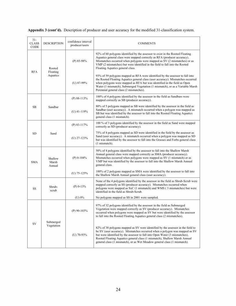
24

Appendix 3 (cont’d). Description of producer and user accuracy for the modified 31-classification system.

31-CLASS CODE

DESCRIPTION confidence interval producer/users COMMENTS

(P) 85-98%

92% of 60 polygons identified by the assessor to exist in the Rooted Floating Aquatics general class were mapped correctly as RFA (producer accuracy). Mismatches occurred when polygons were mapped as SV (2 mismatches) or as VMP (2 mismatches) but were identified in the field to fall into the Rooted Floating Aquatics general class.

RFA Rooted Floating Aquatics

(U) 87-99%

93% of 59 polygons mapped as RFA were identified by the assessor to fall into the Rooted Floating Aquatics general class (user accuracy). Mismatches occurred when polygons were mapped as RFA but was identified in the field as Open Water (1 mismatch), Submerged Vegetation (1 mismatch), or as a Variable Marsh Perennial general class (2 mismatches).

(P) 88-113% 100% of 4 polygons identified by the assessor in the field as Sandbars were mapped correctly as SB (producer accuracy).

SB Sandbar (U) 41-119%

80% of 5 polygons mapped as SB were identified by the assessor in the field as Sandbar (user accuracy). A mismatch occurred when a polygon was mapped as SB but was identified by the assessor to fall into the Rooted Floating Aquatics general class (1 mismatch).

(P) 83-117% 100 % of 3 polygons identified by the assessor in the field as Sand were mapped correctly as SD (producer accuracy).

SD Sand (U) 27-123%

75% of 4 polygons mapped as SD were identified in the field by the assessor as Sand (user accuracy). A mismatch occurred when a polygon was mapped as SD but was identified by the assessor to fall into the Grasses and Forbs general class (1 mismatch).

(P) 0-104%

50% of 4 polygons identified by the assessor to fall into the Shallow Marsh Annual general class were mapped correctly as SMA (producer accuracy). Mismatches occurred when polygons were mapped as SV (1 mismatch) or as VMP but was identified by the assessor to fall into the Shallow Marsh Annual general class.

SMA Shallow Marsh Annual

(U) 75-125% 100% of 2 polygons mapped as SMA were identified by the assessor to fall into the Shallow Marsh Annual general class (user accuracy).

(P) 0-13%

None of the 4 polygons identified by the assessor in the field as Shrub-Scrub were mapped correctly as SS (producer accuracy). Mismatches occurred when polygons were mapped as SxC (1 mismatch) and WMS ( 3 mismatches) but were identified in the field as Shrub-Scrub.

SS Shrub- scrub

(U) 0% No polygons mapped as SS in 2001 were sampled.

(P) 90-103%

97% of 32 polygons identified by the assessor in the field as Submerged Vegetation were mapped correctly as SV (producer accuracy). Mismatches occurred when polygons were mapped as SV but were identified by the assessor to fall into the Rooted Floating Aquatics general class (2 mismatches).

SV Submerged Vegetation

(U) 70-93%

82% of 38 polygons mapped as SV were identified by the assessor in the field to be SV (user accuracy). Mismatches occurred when a polygon was mapped as SV but were identified by the assessor to fall into Open Water (3 mismatches), Rooted Floating Aquatics general class (1 mismatch), Shallow Marsh Annual general class (1 mismatch), or as Wet Meadow general class (1 mismatch).

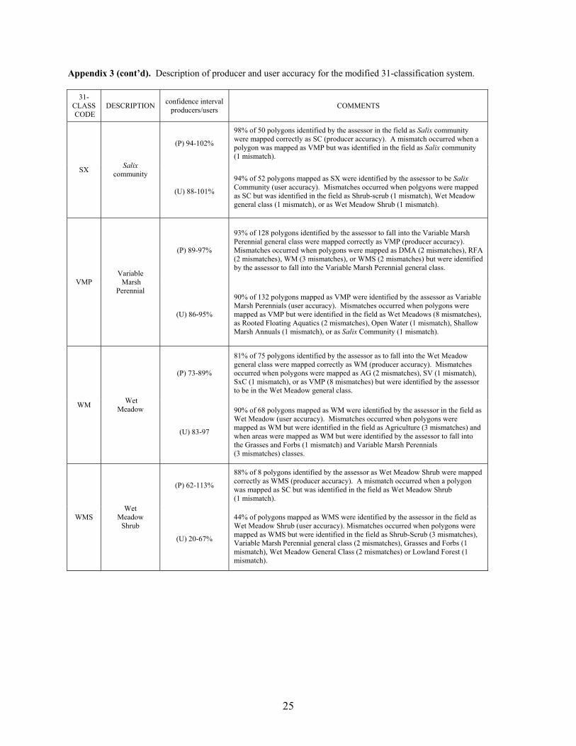
25

Appendix 3 (cont’d). Description of producer and user accuracy for the modified 31-classification system.

31-CLASS CODE

DESCRIPTION confidence interval producers/users COMMENTS

(P) 94-102%

98% of 50 polygons identified by the assessor in the field as Salix community were mapped correctly as SC (producer accuracy). A mismatch occurred when a polygon was mapped as VMP but was identified in the field as Salix community (1 mismatch).

SX Salix community

(U) 88-101%

94% of 52 polygons mapped as SX were identified by the assessor to be Salix Community (user accuracy). Mismatches occurred when polgyons were mapped as SC but was identified in the field as Shrub-scrub (1 mismatch), Wet Meadow general class (1 mismatch), or as Wet Meadow Shrub (1 mismatch).

(P) 89-97%

93% of 128 polygons identified by the assessor to fall into the Variable Marsh Perennial general class were mapped correctly as VMP (producer accuracy). Mismatches occurred when polygons were mapped as DMA (2 mismatches), RFA (2 mismatches), WM (3 mismatches), or WMS (2 mismatches) but were identified by the assessor to fall into the Variable Marsh Perennial general class.

VMP Variable Marsh

Perennial

(U) 86-95%

90% of 132 polygons mapped as VMP were identified by the assessor as Variable Marsh Perennials (user accuracy). Mismatches occurred when polygons were mapped as VMP but were identified in the field as Wet Meadows (8 mismatches), as Rooted Floating Aquatics (2 mismatches), Open Water (1 mismatch), Shallow Marsh Annuals (1 mismatch), or as Salix Community (1 mismatch).

(P) 73-89%

81% of 75 polygons identified by the assessor as to fall into the Wet Meadow general class were mapped correctly as WM (producer accuracy). Mismatches occurred when polygons were mapped as AG (2 mismatches), SV (1 mismatch), SxC (1 mismatch), or as VMP (8 mismatches) but were identified by the assessor to be in the Wet Meadow general class.

WM Wet Meadow

(U) 83-97

90% of 68 polygons mapped as WM were identified by the assessor in the field as Wet Meadow (user accuracy). Mismatches occurred when polygons were mapped as WM but were identified in the field as Agriculture (3 mismatches) and when areas were mapped as WM but were identified by the assessor to fall into the Grasses and Forbs (1 mismatch) and Variable Marsh Perennials (3 mismatches) classes.

(P) 62-113%

88% of 8 polygons identified by the assessor as Wet Meadow Shrub were mapped correctly as WMS (producer accuracy). A mismatch occurred when a polygon was mapped as SC but was identified in the field as Wet Meadow Shrub (1 mismatch).

WMS Wet

Meadow Shrub

(U) 20-67%

44% of polygons mapped as WMS were identified by the assessor in the field as Wet Meadow Shrub (user accuracy). Mismatches occurred when polygons were mapped as WMS but were identified in the field as Shrub-Scrub (3 mismatches), Variable Marsh Perennial general class (2 mismatches), Grasses and Forbs (1 mismatch), Wet Meadow General Class (2 mismatches) or Lowland Forest (1 mismatch).

26

Appendix 4. Recommendations for future accuracy assessments for Land cover/ land use maps produced by UMESC. During photo-interpretation

1. Use a convention of checking with previous data, ground and field notes before making classification decisions.

2. If some important vegetation types need to be mapped at a different MMU, then report the revised MMU for those vegetation/land cover types. The 2001 photos were interpreted with 5700 polygons, 2000 were mapped below 0.75 acres (35%). The 2000 coverage was interpreted with 3700 polygons, 874 were below 0.75 acres (23%). This consistency in mapping over 20% of the map below MMU warrants re-examination of the MMU for some key groups.

3. Another option for MMU may be to rename it as Approximate Minimum Mapping Unit (or AMMU). This allows the photo-interpreter to interpret well below the standard in areas where vegetation may be rapidly changing or disappearing.

Prior to assessment: Selecting sampling points

1. Consider a post-stratification method- where the sample points would be ‘stratified’ based upon the proximity to the boundary of the polygon (actual, not mapped). This process may address a key issue with accuracy assessments, because point proximity to boundary likely increases the variability in the assessment call. Some measure of the point’s minimum acceptable

distance from a polygon boundary would be evaluated for future assessment projects.

2. Consider stratifying the points based upon hydrology rather than on vegetation class per say. Then, depending upon the year that the bathymetry data are taken, the vegetation can be assessed per water level of a particular site.

3. Buffering polygons is an effective means of offsetting spatial error in the map and GPS error for large polygons. Small polygons or narrow linear polygons may be lost during buffering, however. In addition, dynamic systems such as rivers where changes in vegetation over small periods of time are anticipated would likely not benefit from buffering but from highly accurate GPS coordinate records and accurate spatial maps.

4. Points need to be overselected for each class and then decisions of which points to sample are needed if a high concentration of points falls into one area (this reduces oversampling of an area and vegetation type).

5. Consider collecting adhoc accuracy assessment data during the vegetation classification process, perhaps during ground truthing. Collecting additional points would be especially valuable in areas of high vegetation heterogeneity to help troubleshoot for mismatches anticipated as the result of variable vegetation.

6. For river sampling, the largest ‘open water’ polygons or portions of polygons may be excluded from the study unless a particular priority has been placed upon them.

27

7. For river sampling, consider excluding the forested vegetation classes since these classes received the highest producer and user accuracies in this pilot study.

During assessment: Field process and datasheet information

1. Vegetation needs to be sampled at appropriate times. Aquatic vegetation types should be sampled before mid-October and preferably between August and September. Emergent vegetation may be sampled at any time before March and most easily accessed in wintertime. However, as winter approaches and passes, the appearance of a pattern of species distribution may disappear. Terrestrial vegetation is most easily sampled in mid-winter (during leaf off to reduce multi-path error and when access to remote areas is facilitated by frozen ground).

2. A useable key for the LCU types needs to be developed and an understanding of coverage and densities needs to be gained prior to sending an assessor into the field.

3. The assessor needs to establish plots at the minimum mapping unit for each LCU class.

4. Airboats are necessary to access some points in the field.

5. Some ‘terrestrial’ sites are inaccessible by airboat and are not accessible by foot except during the winter when the ice is sufficiently thick to cross. Vegetation types in these areas include: Scirpus, Sparganium, Polygonum, sedge meadows, and some wet meadows and wet meadow shrub types.

6. Garmin 3+ GPS was an effective DGPS for the majority of field sites in the pilot study. Two areas that affected GPS readings were: the bluffs on the Minnesota side in the afternoon, south of the interchange with Highway 26, and b) being position close to Salix communities or densely-canopied forests.

7. Allow for a secondary ‘field call’ and an explanation for why the second choice may be necessary.

8. Require recording relative percent cover for all prominent species, and establish a gradient or code for breaks between significant and non-significant components of a particular vegetation type. The same density modifiers used by the photo-interpreter may be used in the field.

9. Submerged Vegetation can be sampled in some areas well into early December. Trawling with a rake for a certain distance might assess the vegetation more accurately.

10. Use digital photography at every point and either a) photograph in the four cardinal directions or b) photograph directly into the polygon and then directly away from the polygon. Document each photograph in order to avoid confusion during downloading.

11. Obtain permission to access field sites on private property prior to field assessment.

12. To reduce the potential of transcription error from the field sheets to the final database, use field-ready computers with GPS-hookups if such equipment are available. Transcription errors are still likely for GPS coordinates; therefore, maintain a separate sheet with the

28

original map coordinates to help check the data.

Post assessment: Reporting the results

1. Decide whether or not to include genus types that either the map call or the field call did not capture.

2. Decide early whether or not to normalize the data before calculating producer and user accuracy (Stehman and Czaplewski, 1998).

3. Consider using surfaces to generate an idea about spatial error across the map (see reference). A geostatistical package is available for ArcGIS that uses interpolation techniques to generate a spatial error surface on the map (because error is not spread homogeneously across a map).

4. Consider the user needs prior to final publication of the map. Determine whether or not a training workshop is necessary to acquaint the principle users with the 1) land cover classification types and rationale, 2) the way accuracy assessments are run, and 3) the meaning of producer and user accuracies. If the principle users understand how the data work, then they will be able to understand the usefulness of the data.