Theme V – Models and Techniques for

Analyzing Seismicity

Seismicity Rate Changes

David Marsan1 • Max Wyss2

1. Institut des Sciences de la Terre, CNRS, Universite de Savoie 2. World Agency of Planetary Monitoring and Earthquake Risk Reduction

How to cite this article:

Marsan, D., and M. Wyss (2011), Seismicity rate changes, Community Online

Resource for Statistical Seismicity Analysis, doi:10.5078/corssa-25837590. Available

at http://www.corssa.org.

Document Information:

Issue date: 30 January 2011 Version: 1.0

2 www.corssa.org

Contents

1 Why compute seismicity rate changes? . . . . . . . . . . . . . . . . . . . . . . . . . . . . . . . . . . . . . . 3

2 Prerequisite . . . . . . . . . . . . . . . . . . . . . . . . . . . . . . . . . . . . . . . . . . . . . . . . . . . . . 4

3 An introductory case study . . . . . . . . . . . . . . . . . . . . . . . . . . . . . . . . . . . . . . . . . . . . 44 Measuring the significance of a seismicity rate change . . . . . . . . . . . . . . . . . . . . . . . . . . . . . 8

5 Accounting for nonstationary trends in earthquake activity . . . . . . . . . . . . . . . . . . . . . . . . . . 11

6 Searching for a significant change in the earthquake-generating process . . . . . . . . . . . . . . . . . . . . 13

Seismicity rate changes 3

Abstract Earthquake time series can be characterized by the rate of occurrence,which gives the number of earthquakes per unit time. Occurrence rates generallyevolve through time; they strongly increase immediately after a large shock, forexample. Understanding and modeling this time evolution is a fundamental issue inseismology, and more particularly for prediction purposes.

Seismicity rate changes can be subtle, with a slow time evolution, or with agradual onset long after the cause. Therefore, it has proved problematic in manyinstances to assess whether a change in rate is real, i.e., whether it is statisticallysignificant, or not. We here review and describe existing methods developed formeasuring seismicity rate changes, and for testing the significance of these changes.Null hypotheses of ’no change’ are formulated, that depend on the context. Statisticsare then defined to quantify the departure from this null hypothesis. We illustratethese methods with several examples.

1 Why compute seismicity rate changes?

Earthquakes, especially of small to moderate sizes, are generally abundant in activefault zones. Although they do not matter in terms of seismic hazard, their occur-rences are a signature of the state of the crust at seismogenic depths, that cannototherwise be probed or subject to direct measurements. As such, they provide anunique source of information regarding to the mechanical state of potentially dan-gerous seismic asperities.

Changes in seismicity patterns are therefore likely to be correlated to changes instress, as evidenced by aftershock sequences, or by more subtle seismicity dynamicscaused by nucleation processes of large earthquakes. A key issue is then to quantifychanges in the rate of earthquake occurrences, in particular by checking whethersuch changes are actually statistically significant or not. In many applications thechange in rate is obvious, and does not really require any specific analysis; this isclearly the case when considering the whole rupture area of a given mainshock, forwhich the increase in rate is always extremely significant. However, more demandinganalyses are needed when inspecting areas that only experience a weak or mildaftershock triggering, as is the case far off the main fault, or for small areas closeto the fault that are thought of as undergoing stress unloading (eg, stress shadows).Quantitative measures of a change in seismicity are more particularly required whentrying to detect specific patterns (eg, relative quiescence) prior to large shocks, asan attempt to identify precursory phenomena that could be used for earthquakeprediction strategies.

4 www.corssa.org

2 Prerequisite

The reader should be familiar with Poisson processes (Theme III) and seismicitymodels (Theme V), at least for the nonstationary treatment of section 5, beforereading this article.

We will assume throughout this chapter that the earthquake data have beenquality-controlled, in particular that a magnitude of completeness mc has been es-timated, that only earthquakes with magnitudes greater than this mc are kept, andthat the magnitudes are all computed in a consistent way. We refer the reader toHabermann (1987) for a review on how spurious seismicity rate changes can arisefrom artificial effects. Such effects can be detected by considering separate ratechanges for various magnitude bands. We will here only investigate rate changes forthe whole magnitude interval m ≥ mc.

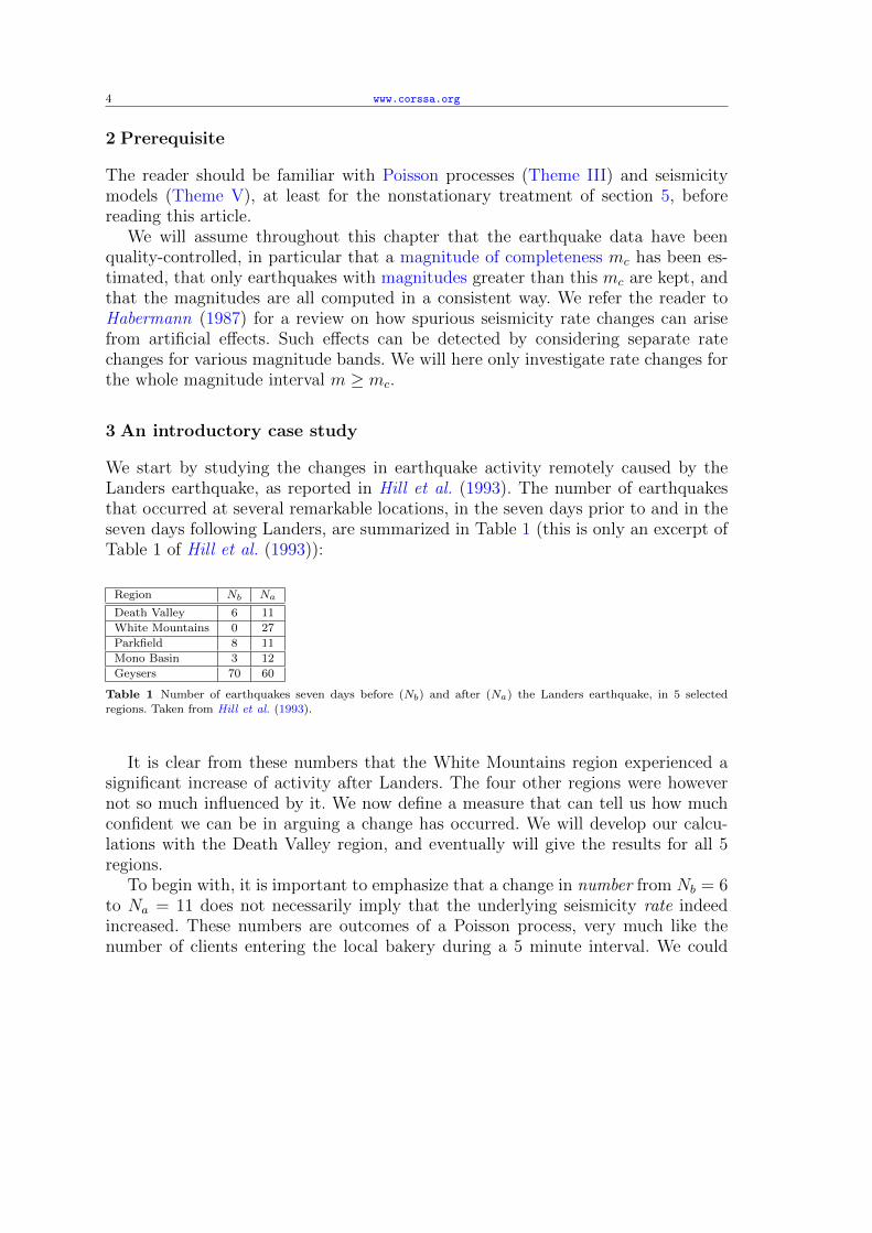
3 An introductory case study

We start by studying the changes in earthquake activity remotely caused by theLanders earthquake, as reported in Hill et al. (1993). The number of earthquakesthat occurred at several remarkable locations, in the seven days prior to and in theseven days following Landers, are summarized in Table 1 (this is only an excerpt ofTable 1 of Hill et al. (1993)):

Region Nb Na

Death Valley 6 11

White Mountains 0 27

Parkfield 8 11

Mono Basin 3 12

Geysers 70 60

Table 1 Number of earthquakes seven days before (Nb) and after (Na) the Landers earthquake, in 5 selected

regions. Taken from Hill et al. (1993).

It is clear from these numbers that the White Mountains region experienced asignificant increase of activity after Landers. The four other regions were howevernot so much influenced by it. We now define a measure that can tell us how muchconfident we can be in arguing a change has occurred. We will develop our calcu-lations with the Death Valley region, and eventually will give the results for all 5regions.

To begin with, it is important to emphasize that a change in number from Nb = 6to Na = 11 does not necessarily imply that the underlying seismicity rate indeedincreased. These numbers are outcomes of a Poisson process, very much like thenumber of clients entering the local bakery during a 5 minute interval. We could

Seismicity rate changes 5

0 0.5 1 1.5 2 2.5 3 3.5 40

0.2

0.4

0.6

0.8

1

1.2

λ

pdf f

(λ)

beforeafter

Fig. 1 Probability density function of the earthquake rate (in 1/day) observed at Death Valley, 7 days before and

7 days after the 1992 Landers earthquake

very well observe that 6 clients came between 11:20 and 11:25, while 11 came between11:25 and 11:30, without necessarily conclude that the second interval is on ensembleaverage nearly twice as busy as the first. Actually, the chance is that the two intervalsare in general equivalent, but today, by pure luck, it happened that Nb = 6 andNa = 11. A null hypothesis could be formulated: the numbers Na and Nb are drawnfrom two independent, identically distributed Poisson laws, i.e., the two intervals areequally busy, and the rate of clients per minute is 6+11

10= 1.7. Then the chance of

observing Nb = 6 and Na = 11 is P (Nb = 6, Na = 11) = e−17 × 8.56

6!× 8.511

11!= 0.91%.

This combination of outcomes will therefore occur 0.43 times per day on average,counting 8 business hours per day, so that our observing it is quite plausible.

We further develop this argument. For any given region, we denote by λb andλa the earthquake rates before and after Landers. As explained in the previousparagraph, these rates are unknown: for example, one could intuitively argue thatthe 6 earthquakes observed at Death Valley in the week prior to Landers couldreasonably be due to a daily rate λb in the [1

7, 3] day−1 range, at the time scale of 1

week. Indeed, the probability to have 6 occurrences in 7 days if λb = 17

day−1 amounts

to P (Nb = 6|λb = 17) = e−1 16

6!= 5.1 × 10−4; equivalently, P (Nb = 6|λb = 3) =

e−21 216

6!= 9×10−5, while it becomes at max P (Nb = 6|λb = 6

7) = e−6 66

6!= 0.161. The

probability density function associated with the rate λ for N earthquakes occurringin a time interval ∆t is

f(λ) = ∆t e−λ∆t(λ∆t)N

N !(1)

6 www.corssa.org

We show in Figure 1 the two pdf (before and after Landers) for Death Valley.The maximum likelihood is given by λ = N

∆t. Using these pdf, we can compute the

probability that the earthquake rate increased by more than a given ratio r, i.e.,

P

(λaλb

> r

)=

∞∫0

dλb fb(λb)

∞∫rλb

dλa fa(λa) (2)

This yields

P

(λaλb

> r

)= 1 − 1

Na! Nb!

∞∫0

dx e−x xNb Γ (Na + 1, rx) (3)

where Γ (n, x) =x∫0dt e−t tn−1 is the incomplete Gamma function. This can be

further generalized to the case where the two time intervals ’before’ and ’after’ donot have the same durations: the last term of Equation 3 must then be changed to

Γ(Na + 1, rx∆ta

∆tb

).

This expression can only be solved numerically. A Matlab program that does thisis given by:

function P=probability_increase(r,Nb,Na,Dtb,Dta)

% estimate the probability that the rate of earthquakes

% ’after’ is at least r times greater than the rate of

% earthquakes ’before’. Nb earthquakes are observed in a time

% duration Dtb before, and Na in Dta after.

if(Nb<25) Nm=max([10 10*Nb]); x=0:Nm*10^(-3):Nm;

else x=Nb-5*sqrt(Nb):sqrt(Nb)*10^(-2):Nb+5*sqrt(Nb); end

tmp=Nb*log(x); if(Nb==0 & x(1)==0) tmp(1)=0; end

tmp=tmp-x-gammaln(Nb+1)+log(gammainc(r*Dta/Dtb*x,Na+1))+log((x(2)-x(1)));

P=1-sum(exp(tmp));

Applying this to the Death Valley case, we find that the probability for an increase

of seismicity (r = 1) is P(λaλb> 1

)= 0.881. The probability for a two-fold increase

(r = 2) is P(λaλb> 2

)= 0.391. The decay of this probability with r is shown in

Figure 2.From these curves, it is easy to determine the 90% confidence interval for r, that

is, the interval r1 < r < r2 so that P (r1) = 5% and P (r2) = 95%. We here find0.80 < r < 4.02. Similarly, the 99% confidence interval is 0.52 < r < 6.79. In bothcases, r values less than 1 are a possibility, as could have been guessed by direct

Seismicity rate changes 7

10−2

100

102

10−10

10−8

10−6

10−4

10−2

100

rate change r

P(>

r)

0 2 4 60

0.2

0.4

0.6

0.8

1

rate change r

P(>

r)

0.881

Fig. 2 Probability of a change in seismicity rate greater than ratio r, for the Death Valley region, in linear andlog-log scales.

inspection of Figure 2. We therefore cannot be confident that the Death Valley regionreally experienced an increase in seismicity rate after the Landers earthquake, atleast at the time scale of one week.

Equivalently, it is interesting to compute the number of earthquakes that should

have occurred in the week following Landers and that would have resulted in P(λaλb> 1

)being greater than a threshold value p. For p = 0.90, we would have needed at least12 earthquakes (only one more than the 11 actually observed), while for p = 0.99this number goes up to 18.

We summarize in Table 2 the results for the five regions. Only the White Moun-tains and the Mono Basin regions can be considered with good confidence (greaterthan 98% in both cases) as having undergone an increase in seismicity rate.

region r = 1 r = 2 r = 5

Death Valley 0.88 0.39 0.02

White Mountains 1.00 1.00 0.93

Parkfield 0.75 0.19 0.0028

Mono Basin 0.989 0.83 0.27

Geysers 0.19 7× 10−7 2× 10−10

Table 2 Probability P(λaλb

> r)

for three values of r, for the 5 regions as in Table 1.

8 www.corssa.org

4 Measuring the significance of a seismicity rate change

We now introduce several statistics that have been or could be proposed to measurethe significance of seismicity rate changes. We keep the same notations as above:before time T of interest (eg, time of occurrence of the Landers mainshock), Nb

earthquakes were observed to occur in a time interval of duration ∆tb, while afterT , we observe Na earthquakes in a time ∆ta. The question is still the same: howsignificant is the rate change that occurred at T , if any? The corresponding nullhypothesis is that there was no change, i.e., before and after are characterized bythe same Poisson process with the same mean rate λ.

4.1 Statistics P and γ (Marsan and Nalbant 2005)

The probability P = P(λaλb> 1

)that λa > λb, is a good and simple measure of how

the two processes characterizing before and after differ of each other. We first discussthe case when ∆ta = ∆tb, for simplicity. It is easy to show in this case that P = 0.5when Na = Nb: there is as much chance that activation (r > 1) or inhibition (r < 1)took place if we observe the same numbers of earthquakes before and after T . Thisvalue P = 0.5 corresponds to the maximum overlap between the two pdf of λa andλb. Departure from λa = λb will therefore result in P departing from 0.5, and goingtowards either 0 if there is a shutdown of activity, or 1 if there is activation.

Remarkably, in the null hypothesis λa = λb, the statistic P follows a uniformrandom law between 0 and 1, as shown in Figure 3. Therefore, one can easily testwhether the computed value P for the specific case under investigation can beexplained by the null hypothesis of ’no change’ or not. For example, if we obtainP = 0.994, then the probability that this value or a greater one could be obtainedby chance if there was no change (null hypothesis) is 1− 0.994 = 0.6%.

Marsan and Nalbant (2005) thus proposed to define the statistic γ as the log (inbase 10) of the departure of P from 0.5:

γ = log10P (4)

if P < 0.5, hence a decrease of activity, or

γ = − log10(1− P) (5)

if P > 0.5, hence an increase of activity. For example, if P = 10−3, then thereis only a 10−3 chance that this apparent decrease or an even stronger one could bedue to pure luck (null hypothesis of no change), and thus γ = −3. On the contrary,if P = 0.999 = 1 − 10−3, then the chance of observing this value or a greater oneby chance is 10−3 also, and γ = +3. The statistic γ therefore provides an easy way

Seismicity rate changes 9

0 0.2 0.4 0.6 0.8 10

0.1

0.2

0.3

0.4

0.5

0.6

0.7

0.8

0.9

1

P

cum

ulat

ive

prob

abili

ty

λ=10

λ=100

λ=1000

Fig. 3 Distribution of the probability P of an increase in seismicity rate, in the hypothesis of no change in rate.

The two intervals before and after are characterized by the same rate λ, which takes three values as indicated onthe graph. A unit time interval is considered for the two periods (∆ta = ∆tb = 1). The distribution was obtained

by running 104 independent simulations.

of telling whether we are close or far from respecting the no-change null hypothesis,and moreover gives the sign of the change. The value of γ can easily be interpretedin terms of a confidence level. For example, a confidence level of 95% correspondsto P < 0.025 or P > 0.975, hence a threshold value of |γ| = 1.6. Similarly, thisthreshold becomes |γ| = 2.3 for a confidence level of 99%.

This statistic is easy to implement:(1) run P=probability_increase(1,Nb,Na,Dtb,Dta); cf above;(2) compute γ as gamma=-sign(P-0.5)*log(min([P 1-P]))/log(10);

When ∆ta and ∆tb are different, the probability P departs from the uniform lawfor the null hypothesis of no change, as shown in Figure 4. However, this departureremains limited, the more so as the two durations are not too different, so thatthe statistic γ can still be used to a good approximation. Alternatively, γ can becomputed by changing P into −0.22P2 + 1.22P if ∆ta

∆tb� 1, or into 0.22P2 + 0.78P

if ∆ta∆tb� 1, cf. Figure 4.

As an example, if we consider the case of the Death Valley region, then P = 0.88,cf. Table 2, and thus γ = +0.92, hence an increase which is not significant. On thecontrary, for the Mono Basin region, P = 0.989, thus γ = +1.96, which can beaccepted as a significant rate change.

10 www.corssa.org

0 0.2 0.4 0.6 0.8 10

0.1

0.2

0.3

0.4

0.5

0.6

0.7

0.8

0.9

1

P

cum

ulat

ive

prob

abili

ty

ta=1

ta=10

ta=100

Fig. 4 Same as in Figure 3, but with ∆tb = 1 and a varying ∆ta as indicated on the graph. For ∆ta 6= ∆tb, the

probability P slightly departs from a uniform law: a good fit of the cumulative probability is given by Pr(P < x) =−0.22x2 + 1.22x, for both ∆ta = 10 and ∆ta = 100.

4.2 Statistic β of Matthews and Reasenberg (1988)

Instead of considering the full probability densities as for example shown in Figure 1,one can compute the difference between the observed number Na and the expectednumber Nb × ∆ta

∆tb, and rescale it by the typical dispersion (i.e., standard deviation)√

Nb × ∆ta∆tb

. This gives the statistic

β =Na − Λ√

Λ(6)

with Λ = Nb ×∆ta∆tb

(7)

Note that a symmetric measure could be proposed as Λ−Nb√Λ

and Λ = Na × ∆tb∆ta

,

which is equal to β when ∆ta = ∆tb. For the Death Valley region, we obtain β =+2.04, while for the Mono Basin region β = +5.19. As can be seen with this example,large β values, sometimes greater (in absolute value) than 5, are needed to makesure the rate change is effectively significant. Such a large critical value is necessaryhere because the numbers Nb are small.

The translation of β into a probability can be done in the limit of large numbersof earthquake occurrences, for which the Poisson distribution tends to a Gaussianlaw. In the null hypothesis of no change, β is distributed like a Gaussian with zero

Seismicity rate changes 11

mean and unit standard deviation. Thus, for a positive β, the probability to obtaina greater value is 1

2− 1

2erf(β/

√2) where erf is the error function, while for a negative

β the probability to obtain a smaller value is 12

+ 12erf(β/

√2).

It can be argued that, while being very simple to compute, the β-statistic isperhaps not the best choice: a symmetric version (as is the case of Z, cf. below) wouldbe more appropriate, and the significance level of the rate change is not directlygiven by the value of β. Moreover, the underlying assumption of large numbers ofearthquakes limits its use.

4.3 Statistic Z of Habermann (1981)

A measure was proposed by Habermann (1981) as

Z =Na ∆tb − Nb ∆ta√Na ∆t2b + Nb ∆t2a

(8)

This is very similar to the β statistic, or, more exactly, is a symmetrical versionof it, i.e., the denominator depending equally on both time intervals. As with the βstatistic, in the limit of large numbers Na and Nb, Z is distributed like a Gaussianlaw with zero mean and unit standard deviation, in the null hypothesis of no change.A derivation of this result can be found in Marsan and Nalbant (2005). Note thatthe original Z statistic as proposed by Habermann (1983) has the sign reversed fromthe one defined in Equation 8. We changed this sign to be coherent with the otherstatistical measures.

We compute Z for the Death Valley region: Z = +1.21, and for the Mono Basinregion: Z = +2.32. The change can be considered as significant if |Z| > 2.

5 Accounting for nonstationary trends in earthquake activity

So far we have compared the observed Na earthquakes after the time of interestT to the Nb occurrences before. The rationale of this comparison is that, if therewere indeed no change, then we would expect Na to be a random draw of the samePoisson process that generated Nb. However, this expectation must be reexamined ifwe know the earthquake activity is following a nonstationary trend at time T . Thecase of mainshock doublets or even multiplets is here particularly important: if wewant to map the changes in seismicity (and thus of stress) brought by the secondmainshock M2, we first need to understand how the seismicity was evolving prior toit. Since the first mainshock M1 initiated an aftershock sequence, this activity waslikely to be decaying at the time of M2. A model is therefore required to ’propagate’

12 www.corssa.org

the ’normal’ aftershock activity of M1 past the occurrence of M2, so to comparebetween the observed earthquake rate and this predicted rate.

There are typically two ways to address the issue of nonstationarity. The moretraditional method is to first decluster the dataset, which in principle should resultin a stationary dataset for which the quantities described in Section 4 can then beapplied. However, removing aftershocks from the earthquake catalog is in most casesnot desirable. For example, testing whether a change in Coulomb stress caused bya mainshock implied a change in seismicity rate obviously requires to consider theaftershocks of this mainshock.

The other solution is to model the earthquake-generating process and its timeevolution, knowing the history of the process up to time T , and then use this modelto guess how λa should be distributed if there were no other change (apart fromthe ’normal’ trend) at time T . This approach was developed in Marsan (2003). Themain issue is to propose a good model that can well explain the evolution of thetime series up to time T , and to extrapolate this time series between T and T + ta.

As an example, Figure 5 extracted from Daniel et al. (2008) shows the case ofthe June 2000, Iceland, doublet, in which two very similar Ms6.6 vertical, strike-slipearthquakes occurred within 3.5 days and ∼15 km of each other. In this Figure, theseismicity rate at the Hengill triple junction (about 30 to 50 km away from the twoearthquakes) is shown, after correction for completeness issues (white bars). Time0 is 00:00, 17th of June, hence only a few hours before the occurrence of the firstmainshock. This mainshock initiated an aftershock sequence in this zone, althoughwe are far from the rupture zone itself. This sequence is modeled with an Omori-Utsu law; the fit is done from the time of the first mainshock to the time T of thesecond, and then extrapolated to t > T . A clear departure in seismicity rate fromthis trend just after the 2nd mainshock is observed, lasting for about 5 hours only.This increase in rate from the expected rate can then be tested using the variousstatistic described in Section 4.

The method for estimating rate changes in the context of nonstationary trendsis then:

1. knowing earthquake activity up to time T , fit a model λ̂(t) to the seismicity rate;

2. extrapolate λ̂(t) to the time interval of duration ∆ta of interest;3. deduce from this extrapolation a pdf f(λ) for the expected λ for this interval.

The simplest pdf is a Dirac f(λ) = δ(λ − λ̂) with its atom on the extrapolatedvalue, but accounting for estimate uncertainties during the parameterization ofthe model λ̂(t), or even for the simple fact that in general the rate extrapolatedover the whole interval ∆ta is not constant, would result in a more complex pdf;

4. use the statistic P and associated γ, with f(λ) replacing fb(λb):

Seismicity rate changes 13

Fig. 5 Black bars: seismicity rates observed at Hengill Triple Junction frm 00:00 on June 17, 2000. The occurrencetimes of the two Ms6.6 mainshocks are indicated by the first bar and by the vertical dotted line, respectively.

White bars: same as with the black bars, but after correcting for completeness issues. The rate is then for m ≥ 0

earthquakes. Gray curve: best Omori-Utsu law fitted using the time interval between the two mainshock, thatmodels the aftershock sequence in this zone caused by the first mainshock. It is further extrapolated after the

second mainshock. Extracted from Daniel et al. (2008).

P = 1 − 1

Na!

∞∫0

dx f(x

∆ta

)Γ (Na + 1, x) (9)

6 Searching for a significant change in the earthquake-generating process

In many applications, the rate change is estimated at a particular time T of interest,typically the occurrence of a mainshock. However, one can also be interested inchecking whether there exists a significant change within a given interval, without apriori knowing the exact time T at which this change occurs. Then T is considered asan unknown parameter in this problem. Sophisticated methods have been proposedto address this problem (Ogata 1988, 1989, 1992, 1999, 2001), with a particular

14 www.corssa.org

emphasis on searching for anomalous seismicity rate decreases precursory to largeshocks.

With this approach, one is interested in detecting the time at which the earthquake-generating process is significantly modified. To summarize, a model of seismicity isfitted to the data up to time T , and then extrapolated to later times t > T . Depar-ture of the data at t > T from this extrapolation is then sought for. An optimizationis performed to maximize this departure, by changing the change-point T . Finally,for the optimized T , the significance of the departure between the data and theextrapolation is computed.

To illustrate this, and further detail the method, we discuss the case of theseismicity in the Aleutian arc from 1965 to 1989, taken from Ogata (1992), cf.Figure 6. In this analysis, a temporal ETAS model was fit to the data, separatelyfor two distinct time intervals. The second time interval extends from some timein the year 1965 to 1975 (vertical dashed line in Figure 6). This model gives the

expected earthquake rate λ̂(t) at any time t. Integrating this rate over time since a

starting time T gives Λ̂(T, t) =t∫Tds λ̂(s), the expected number of earthquakes that

should have occurred, according to the model, between T and t.If the model is good, then the actual number of earthquakes N(T, t) between

T and t should result from a Poisson process with mean rate 1 when consideringthe transformed time τ = Λ̂(T, t) instead of the real time t. A plot of N(T, t) vs.τ should thus show a curve close to a straight line of slope 1. Departure of N(T, t)from this line therefore indicates that the model does not correctly explain the data.A measure can be proposed to test how significant this departure is (Ogata 1992):

ξ =N(T, t)− Λ̂(T, t)√Λ̂(T, t) + Λ̂(T, t)2/N0

(10)

where N0 is the number of earthquakes that occurred in the fitting interval. Theterm related to N0 in the denominator of Equation 10 is effectively a correction termthat accounts for parameter uncertainties when fitting the model; such uncertaintiesare reduced when N0 increases. Apart from this correction, ξ is very similar to theβ statistic. Moreover, ξ is distributed like a Gaussian law with zero mean and unitstandard deviation when the model well approximates the data. Optimization thenamounts to find the best date for the changing-point T , so that the departure is themost significant.

A simpler approach to finding the best change-point date T is proposed in Wyssand Habermann (1988). It consists in computing the Z statistic for a varying time T ,considering as before the earthquakes occurring between an initial time t0 and T , andas after the earthquakes between T and an ending time t1. The latter is typically the

Seismicity rate changes 15

Fig. 6 Cumulative number of mb ≥ 5.1 earthquakes in the Aleutian arc (40o < latitude < 80o and 170oE <

longitude < 160oW) from 1965 to 1989, vs. time (left) and vs. transformed time (right). The seismicity is modeled

using a temporal ETAS model, with two set of parameters fitted over two distinct time intervals as shown with thevertical dashed lines (the first interval is all contained in 1965, year of the Mw8.7 great Rat Island earthquake). The

model is then extrapolated past the second dashed line (year 1975) for constructing the transformed-time graph.

On this graph, departure of the data from the central dotted curve past the lower-most dotted curve indicatesa significant shutdown of activity, compared to what would have been predicted had the earthquake-generating

process remained statistically the same after 1975. This relative quiescence lasts several year, up to the time of the

1986 Ms7.7 Andoreanof Islands earthquake (shown by the upward pointing arrow). Taken from Ogata (1992).

date of a large shock of interest, when searching for precursory quiescence patterns.The most significant Z is then selected. This first requires to decluster the data, asalready mentioned when introducing the Z statistic.

Acknowledgements Many thanks to Katerina Orfanogiannaki and an anonymousreviewer for their constructive comments. D. M. benefited from financial support byANR project ASEISMIC.

References

Daniel, G., D. Marsan, and M. Bouchon (2008), Earthquake triggering in southern iceland following the june 2000

ms 6.6 doublet, J. Geophys. Res., 113 (B05310). 12, 13

Habermann, R. E. (1981), Precursory seismicity patterns: Stalking the mature seismic gap, in Earthquake prediction- An international review, edited by D. W. Simpson and P. G. Richards, pp. 29–42, American Geophysical Union.

11Habermann, R. E. (1983), Teleseismic detection in the aleutian island arc, J. Geophys. Res., 88, 5056–5064. 11Habermann, R. E. (1987), Man-made seismicity rate changes, Bull. Seismol. S([0 3.5],A1*exp(alpha1*[0 3.5]),’k’)

oc. Am., 77, 141–159. 4

16 www.corssa.org

Hill, D. P., P. A. Reasenberg, A. Michael, W. J. Arabaz, G. Beroza, D. Brumbaugh, J. N. Brune, R. Castro,S. Davis, D. dePolo, W. L. Ellsworth, J. Gomberg, S. Harmsen, L. House, S. M. Jackson, M. J. S. Johnston,

L. Jones, R. Keller, S. Malone, L. Munguia, S. Nava, J. C. Pechmann, A. Sanford, R. W. Simpson, R. B. Smith,M. Stark, M. Stickney, A. Vidal, S. Walter, V. Wong, and J. Zollweg (1993), Seismicity remotely triggered by

the magnitude 7.3 Landers, California, earthquake, Science, 260 (5114), 1617–1623. 4

Marsan, D. (2003), Triggering of seismicity at short time scales following californian earthquakes, J. Geophys. Res.,108, 2266. 12

Marsan, D., and S. S. Nalbant (2005), Methods for measuring seismicity rate changes: A review and a study of

how the m-w 7.3 landers earthquake affected the aftershock sequence of the m-w 6.1 joshua tree earthquake,Pageoph, 162 (6-7), 1151–1185. 8, 11

Matthews, M. V., and P. A. Reasenberg (1988), Statistical methods for investigating quiescence and other temporal

seismicity patterns, Pageoph, 126, 357–372. 10Ogata, Y. (1988), Statistical models for earthquake occurrences and residual analysis for point processes, J. Am.

Stat. Assoc., 83 (401), 9–27. 13

Ogata, Y. (1989), Statistical model for standard seismicity and detection of anomalies by residual analysis, Tectono-phys., 169, 159–174. 13

Ogata, Y. (1992), Detection of precursory relative quiescence before great earthquakes trhough a statistical model,

J. Geophys. Res., 97 (B13), 19,845–19,871. 13, 14, 15Ogata, Y. (1999), Seismicity analysis through point-process modeling: A review, Pure Appl. Geophys., 155, 471–507.

13Ogata, Y. (2001), Increased probability of large earthquakes near aftershock regions with relative quiescence, J.

Geophys. Res., 106 (B5), 8729–8744. 13

Wyss, M., and R. E. Habermann (1988), Precursory quiescence before the august 1982 stone canyon, san andreasfault, earthquakes, Pure Appl. Geophys., 126 (2-4), 334–356. 14