This is a repository copy of Theoretical and empirical estimates of mean-variance portfolio sensitivity.

White Rose Research Online URL for this paper:http://eprints.whiterose.ac.uk/79158/

Version: Accepted Version

Article:

Palczewski, A and Palczewski, J (2014) Theoretical and empirical estimates of mean-variance portfolio sensitivity. European Journal of Operational Research, 234 (2). 402 - 410. ISSN 0377-2217

https://doi.org/10.1016/j.ejor.2013.04.018

eprints@whiterose.ac.ukhttps://eprints.whiterose.ac.uk/

Reuse

Unless indicated otherwise, fulltext items are protected by copyright with all rights reserved. The copyright exception in section 29 of the Copyright, Designs and Patents Act 1988 allows the making of a single copy solely for the purpose of non-commercial research or private study within the limits of fair dealing. The publisher or other rights-holder may allow further reproduction and re-use of this version - refer to the White Rose Research Online record for this item. Where records identify the publisher as the copyright holder, users can verify any specific terms of use on the publisher’s website.

Takedown

If you consider content in White Rose Research Online to be in breach of UK law, please notify us by emailing eprints@whiterose.ac.uk including the URL of the record and the reason for the withdrawal request.

Theoretical and empirical estimates of mean-variance

portfolio sensitivity

Andrzej Palczewski

Faculty of Mathematics, University of Warsaw, Poland

Jan Palczewski∗

School of Mathematics, University of Leeds, Leeds LS2 9JT, UK

Abstract

This paper studies properties of an estimator of mean-variance portfolio weights

in a market model with multiple risky assets and a riskless asset. Theoretical for-

mulas for the mean square error are derived in the case when asset excess returns

are multivariate normally distributed and serially independent. The sensitivity of

the portfolio estimator to errors arising from the estimation of the covariance ma-

trix and the mean vector is quantified. It turns out that the relative contribution

of the covariance matrix error depends mainly on the Sharpe ratio of the market

portfolio and the sampling frequency of historical data. Theoretical studies are

complemented by an investigation of the distribution of portfolio estimator for

empirical datasets. An appropriately crafted bootstrapping method is employed

to compute the empirical mean square error. Empirical and theoretical estimates

are in good agreement, with the empirical values being, in general, higher. (JEL:

C13, C52, G11)

Keywords: Investment analysis, asset allocation, mean-variance portfolio,

estimation error, bootstrap

The mean-variance framework, introduced by Markowitz (1952), opened a

new era in asset management. The selection of optimal portfolio was formulated

as seeking a balance between the risk, measured by the variance of the portfolio

return, and the gain, measured by the expectation of the return. A mean-variance

∗Corresponding author, tel. +44 113 34 35180, fax. +44 113 34 35090

Email addresses: A.Palczewski@mimuw.edu.pl (Andrzej Palczewski),

J.Palczewski@leeds.ac.uk (Jan Palczewski)

Preprint submitted to Elsevier December 24, 2012

investor maximizes the objective function (utility)

B(w) = µT w − γ2

wTΣw, (1)

where w denotes portfolio holdings specified in terms of fractions of the wealth,

and the constant γ > 0 is the investor’s risk aversion parameter. It is assumed im-

plicitly that future excess returns of risky assets have a known multidimensional

distribution with the vector of means denoted by µ and the covariance matrix de-

noted by Σ. This assumption is not satisfied in practice. Estimation of parameters

of future asset returns is an essential step in the application of the mean-variance

paradigm in practical finance. The impact of estimation errors on the Markowitz

optimization procedure has been intensively studied for over 30 years. The litera-

ture can be split into two areas. The first one is concerned with the performance

of the estimated portfolio, e.g., the loss of utility, i.e., the difference between the

value of the objective function for the true optimal portfolio and its estimate (see

Frost and Savarino (1986), Kan and Zhou (2007)). The second area studies statis-

tical properties of portfolio estimators.

Our paper belongs to the strand of literature which directly addresses the dis-

tribution of the optimal portfolio estimator. The first result in this direction is

due to Dickinson (1974), who finds approximate confidence intervals for portfo-

lio weights in a two-asset framework. These results are extended by Jobson and

Korkie (1980), who derive approximate asymptotic distributions of the Sharpe ef-

ficient portfolio (the tangency portfolio). Monte Carlo verification of these results

shows that the expectations of the computed asymptotic distributions are close to

the finite sample quantities whereas the variances and covariances are burdened

with a significant error. Statistical tests based on finite-sample distributions, in

the model without a riskless asset, are collected in Jobson and Korkie (1989), and

Britten-Jones (1999).

A view from a different angle on the stability of portfolio weights is promoted

2

by Best and Grauer (1991a, 1991b). Their analytical formulas estimate the change

of optimal portfolio weights caused by a deterministic perturbation of the mean of

asset returns. They show that the sensitivity of portfolio weights to the changes in

asset means depends not only on the smallest eigenvalue of the covariance matrix

but also on the ratio of the largest to the smallest eigenvalue. We extend these

results by studying the effect of the estimation errors of the mean and covariance

matrix given by their exact sample distributions, instead of fixed perturbations.

This paper approaches the estimation of portfolio weights with three main

questions in mind: How to measure errors of a portfolio estimator so that the

performance of various estimators can be easily compared? What are the main

sources of estimation errors? And finally, what is the influence of the estimator of

the covariance matrix on the stability of the portfolio estimator?

We take a view of an investor who rebalances his portfolio regularly following

recommendations given by a solution to the mean-variance optimization problem

with the mean of excess returns and their covariance matrix estimated from market

data. Such an investor either follows the recommendations blindly or employs sta-

tistical tests to detect times when the rebalancing of portfolio is necessary due to

a change of the asset return distribution. Portfolio estimation errors cause unnec-

essarily large and frequent trading and blow up confidence intervals for portfolio

weights lowering the power of statistical tests of portfolio optimality. The stabil-

ity of the optimal portfolio estimator is, therefore, of paramount importance. We

design a measure that combines errors of separate portfolio weights into a single

number: we take the expected squared distance of the estimated portfolio from

the optimal one. Despite its simplicity, this measure provides a good proxy for the

variability of separate weights. Empirical tests for a number of practical datasets

show that this measure is proportional to the average size of confidence intervals

for single weights. It is also closely related to the turnover which is proportional

3

to the transaction costs levied on an investor rebalancing the portfolio on a regular

basis.1

This paper makes three contributions. The first contribution is the derivation of

closed-form formulas that relate the stability of portfolio estimator to the mean and

the covariance matrix of asset returns (analogous formulas in the model without a

riskless asset can be derived from results in Mori (2004) and Okhrin and Schmid

(2006)). Our results rely on finite sample distributions of the mean and covariance

estimators. Using exact distribution of portfolio weights, we are able to extend the

findings of Best and Grauer (1991a, 1991b). Their sensitivity analysis revealed

important culprits of the portfolio weight instability: the smallest eigenvalue of

the covariance matrix and the ratio of the largest to the smallest eigenvalue. We

show that this relation is more intricate and depends on the whole spectrum of the

covariance matrix as well as on the vector of the means.

Our second contribution is the quantification of the impact of estimation errors

of the means on the portfolio weights. It is a common wisdom that the means

play the main role in the destabilization of the portfolio weights (see Best and

Grauer (1991a, 1991b, 1992)). Chopra and Ziemba (1993) claim that ”errors

in means are 11 times as damaging as errors in variances and over 21 times as

damaging as errors in covariances”. This view is further supported by DeMiguel,

Garlappi and Uppal (2009). In our extensive study of eight datasets2 ranging from

domestic to international bond and stock markets with as few as 5 assets to as

many as 17 assets, estimation errors of the covariance matrix account typically for

14% of the variability of portfolio weights with weekly sampling and 28% with

monthly sampling of historical prices (and these quantities are independent of

1We use the framework for portfolio rebalancing and the definition of turnover presented in

DeMiguel, Garlappi and Uppal (2009).2Six datasets of stock prices come from Kenneth French’s data library. Two datasets comprise

bond market data, the courtesy of Merrill Lynch & Co.

4

the number of samples).3 This implies that the improvement of the sample mean

estimator, for example, by shrinkage or Bayesian techniques (see Jorion (1991),

Kan and Zhou (2007)), must still leave a great deal of instability in the Markowitz

optimization procedure (empirical results supporting this view can be found in

DeMiguel, Garlappi and Uppal (2009)).

A by-product of our analysis is the observation that the relative impact of

estimation errors of the covariance matrix on the variability of portfolio weights

is market specific. The main driving forces are the Sharpe ratio of the market

portfolio and the frequency of asset price sampling. The fraction of the variability

of portfolio weights caused by the covariance matrix estimation errors is well

approximated by a parameter (CCF) which is a function of the market portfolio’s

Sharpe ratio, the sampling frequency and the sample size.

Our third contribution is the assessment of the impact of assumptions about

asset returns distribution on properties of portfolio weights estimator. Our the-

oretical results require that asset returns are serially independent and multivari-

ate normally distributed. These assumptions are common in statistical literature

on portfolio estimators, but they have been heavily criticized for decades (espe-

cially for higher sampling frequencies of returns, see, e.g., Fama (1965), Pagan

(1996), McNeil et al.(2005)). Using the block bootstrap methodology (Hardle

et al.(2003)), we explore the empirical distribution of the portfolio estimator. This

method preserves not only the marginal distribution but also the serial correla-

tion in the time series of asset returns. Surprisingly, the unrealistic distributional

assumptions have very limited effect on the results on portfolio weight stability:

empirical and theoretical computations are generally in good agreement.

3These values were obtained under the assumption that the Sharpe ratio of the market portfolio

equals 1. If this Sharpe ratio is lowered to 0.5, estimation errors of the covariance matrix account

for around 7% (weekly sampling) and 15% (monthly sampling) of portfolio weights variability.

5

The rest of the paper is organized as follows. In Section 1, we present the

mean-variance optimization framework and estimators of the mean and covari-

ance matrix of asset returns. In Section 2, we introduce a measure of stability of

portfolio weights and derive exact analytical formulas quantifying this stability.

These results and their conclusions are verified by empirical studies in Section 3.

In the Electronic Supplement, Section A quotes less known statistical results re-

quired for the proof of the main theorem in Section B. Section C provides details

about the data used in empirical studies.

1. Mean-variance portfolio selection

The market comprises p risky assets and a riskless asset. Future excess returns

of the risky assets, i.e., the returns over the return of the riskless asset, are modeled

by a normally distributed vector R = (R1, . . . ,Rp)T with the expectation µ and the

non-singular covariance matrix Σ = [σi j]. An investor describes his portfolio by

a vector w = (w1, . . . ,wp)T ∈ Rp of fractions of the total capital invested in risky

assets. The proportion 1 − wT 11, where 11 is the vector of ones, is invested in

the riskless asset. The expected excess return of the portfolio equals µT w and its

variance is wTΣw. According to Markowitz mean-variance framework, an investor

looks for a portfolio that balances the return with the risk, see (1). In the present

setting this leads to the maximization of the objective function B(w) = µT w −γ

2wTΣw over portfolio weights w ∈ R

p. This problem has a unique solution:

w∗ =1

γΣ−1µ. (2)

In practice, true moments of the distribution of future excess return R are un-

known to investors and are estimated from the market data. The data from time

0 to T is used for the estimation and the time from T to T + 1 is the investment

period, i.e., the time is measured in units equal to the length of the investment

period. Let n + 1 be the number of equidistant sampling times: 0,∆, 2∆, . . . , n∆,

6

where ∆ = T/n. Denote by ri the logarithmic return over period [(i − 1)∆, i∆],

i = 1, . . . , n. Assume that returns are multivariate normally distributed N(∆µ,∆Σ)

and independent. The mean and the covariance matrix of R (per unit time) are

approximated via maximum-likelihood estimators:

µ∆ =1

n∆

n∑

t=1

rt, (3)

Σ∆ =1

n∆

n∑

t=1

(rt − µ∆)(rt − µ∆)T . (4)

Theorem 3.2.2 in Anderson (2003) implies that the estimator µ∆ is normally dis-

tributed N(µ,Σ/(n∆)) = N(µ,Σ/T ) and independent from Σ∆ which has a Wishart

distribution 1nWp(Σ, n − 1).

The sample mean (3) and the sample covariance matrix (4) are the building

blocks of estimators of optimal portfolio weights discussed in the next section.

2. Properties of portfolio weights estimator

In this section we present theoretical results on statistical properties of esti-

mated portfolio weights. Unlike the papers by Mori (2004) or Okhrin and Schmid

(2006), we do not provide the full covariance matrix of the portfolio weight esti-

mator (although it can be computed using similar methods). Instead, we study a

simpler quantity (the MSE introduced below) which is a single number allowing

for straightforward comparison between estimation methods and, as we show in

Section 3, offers a good proxy for the variability of portfolio weights.

2.1. Mean square error

Mean square error is a well-established method of measuring the statistical

error (see, e.g., Hocking (2003) and, in the context of mean-variance portfolio

theory, Broadie (1993)). In the framework of portfolio optimization the mean

square error is given by the formula

MS E(w) = E‖w − w∗‖2,

7

where w∗ is the optimal portfolio (see (2)), w is the estimated portfolio and ‖w‖ =

(∑p

i=1w2

i )1/2 denotes the Euclidean norm. The average (expectation) is taken over

the distribution of the data sample used for the estimation of the mean and the

covariance matrix. The MS E measures the sensitivity of the optimization proce-

dure to the estimation errors: a high value corresponds to a low precision of the

portfolio weights estimates.

The mean square error can be decomposed into a sum of two terms:

MS E(w) = E‖w − Ew‖2 + ‖Ew − w∗‖2.

The first term is the sum of variances of the portfolio weights estimator w, i.e., the

trace of the covariance matrix of w (Mori (2004) and Okhrin and Schmid (2006)

derive formulas for this covariance matrix in the case without a riskless asset).

The second term of the above formula is the squared norm of the bias Ew − w∗.

We will restrict our attention to unbiased estimators, hence this term will vanish.

There are many methods (e.g., APT or the Black-Litterman approach) that de-

liver estimators of the mean of future returns which are much more stable than the

maximum-likelihood estimator µ. An insight into improvements these methods

can offer for the stability of portfolio weights is gained by studying the portfolio

optimization problem of an investor who knows the true future expected returns

vector µ and uses past returns to estimate the covariance matrix only.

An unbiased estimator of the optimal portfolio weights, provided the true

mean is known and the covariance matrix is approximated via maximum-likelihood

estimator, is given by the formula (see Theorem B.1 in the Electronic Supplement)

wµ =1

γ

n − p − 2

n(Σ∆)

−1µ.

The factorn−p−2

nremoves the bias from the estimator Σ−1

∆of the inverse of the

sample covariance matrix. Theorem B.1, in the Electronic Supplement, implies

8

the following formula for the mean square error of the above estimator:

MS E(wµ) =n − p

(n − p − 1)(n − p − 4)‖w∗‖2

+1

γ2

n − p − 2

(n − p − 1)(n − p − 4)tr(Σ−1)µTΣ−1µ.

(5)

This error decreases to zero as the number of samples n grows to infinity, but it is

independent of the sampling time interval ∆. By decreasing ∆ and increasing n,

one can make MS E(wµ) arbitrarily close to zero. Unfortunately, for high sampling

frequencies (small ∆) the serial correlation of empirical returns increases and their

distribution diverges from the normal distribution (see, e.g., Fama (1965) and Mc-

Neil et al.(2005) [Chapters 3 and 4]), which invalidates not only the above formula

but also the estimation procedure of parameters of future returns.

If the mean-variance optimal portfolio is computed with the mean and the co-

variance matrix estimated from market data, an unbiased estimator of the optimal

portfolio weights is given by the formula

w =1

γ

n − p − 2

n(Σ∆)

−1µ∆. (6)

The mean square error for this estimator is provided by the following expression

(see Theorem B.1 in the Electronic Supplement):

MS E(w) =n − p

(n − p − 1)(n − p − 4)‖w∗‖2

+1

γ2

n − p − 2

(n − p − 1)(n − p − 4)tr(Σ−1)µTΣ−1µ

+(n − p − 2)2

γ2n∆(n − p − 1)(n − p − 4)tr(Σ−1)

(

1 +p

n − p − 2

)

.

(7)

The sum of the first two terms of the above formula is equal to the mean square

error for a portfolio estimator using the true mean. The third term combines er-

rors due to the use of the estimated mean. Notice that this term sees hardly any

improvement when the frequency of sampling is increased (∆ is decreased and n

9

is increased) since, approximately (for large n), it equals

1

γ2n∆tr(Σ−1) =

1

γ2Ttr(Σ−1).

2.2. Relation to properties of market portfolio

To compute the mean square error, formulas (5) and (7), one has to know the

true parameters of future returns as well as the true optimal portfolio. These are

liable to large estimation errors and, in effect, result in imprecise estimates of the

mean square error. In this subsection we show that the mean µ of the future returns

and the true optimal portfolio w∗ can be replaced by appropriate statistics for the

market portfolio (which are much easier to compute from market data).

In an ideal situation, when all investors assume the same parameters of the

future returns distribution and use the mean-variance criterion for choosing their

portfolios (possibly with different risk-aversion coefficients), the mutual fund the-

orem implies that they divide their wealth between the market portfolio wm (also

called the tangency portfolio) and the riskless asset. Denote by γm > 0 the mar-

ket risk aversion (the risk aversion for which wm is the optimal portfolio, i.e., the

investment in the riskless asset is nil). It is then easy to verify that the following

identities hold:

µ = γmΣwm, w∗ =γm

γwm, and µTΣ−1µ = γ2

mwTmΣwm.

Inserting these values into (5) gives

MS E(wµ) =γ2

m

γ2

(

n − p

(n − p − 1)(n − p − 4)‖wm‖2

+n − p − 2

(n − p − 1)(n − p − 4)tr(Σ−1)wT

mΣwm

)

. (8)

The mean square error is proportional to the squared ratio of the market risk aver-

sion and the investor’s risk aversion. The first term depends on the number of

risky assets, the number of samples and the norm of the market portfolio. In

10

practical applications the market portfolio has non-negative weights (see Litter-

man (2003)[Chapter 8]), which implies ‖wm‖ ≤ 1. The second term depends on

the variance of the market portfolio wTmΣwm and the trace of the inverse of the

covariance matrix (the sum of inverses of eigenvalues of Σ).

The mean square error (7), when both parameters of future returns are esti-

mated from the data, can be written in the following way:

MS E(w) = MS E(wµ) +(n − p − 2)2

γ2n∆(n − p − 1)(n − p − 4)tr(Σ−1)

(

1 +p

n − p − 2

)

. (9)

The additional term depends only on the trace of the inverse of Σ, being indepen-

dent of the properties of the market portfolio.

2.3. Impact of the structure of covariance matrix

Assume first that assets are independent and, without loss of generality, or-

dered from the most to the least risky. The covariance matrix has its eigenvalues,

from the largest λ1 to the smallest λp, on the diagonal and zeros off diagonal. The

first term of the formula (8) depends on the market portfolio composition and the

sample size. The covariance matrix affects only the second term which can be

rewritten in the following way:

γ2m

γ2

n − p − 2

(n − p − 1)(n − p − 4)tr(Σ−1)wT

mΣwm

=γ2

m

γ2

n − p − 2

(n − p − 1)(n − p − 4)

(

p∑

i=1

1

λi

)(

p∑

i=1

w2m,iλi

)

. (10)

First two factors do not depend on the covariance matrix. The third factor is mostly

determined by the inverses of smallest eigenvalues. The last factor is a sum of the

eigenvalues multiplied by the squares of portfolio weights. The main contribution

to this value comes from the products of large eigenvalues and portfolio weights.

A wide range of eigenvalues should therefore lead to a high mean-square error.

Indeed, one has(∑p

i=11λi

)(∑p

i=1w2

m,iλi

)

≥ w2m,1λ1/λp. This shows that the ratio of

11

the largest to the smallest eigenvalue is one of the driving factors of the mean-

square error MS E(wµ).4

The above analysis can be extended to a model with dependent assets. To this

end, we rewrite the expression tr(Σ−1)wTmΣwm in the eigenbasis of Σ:

tr(Σ−1)wTmΣwm = tr(Σ−1

D )wTDΣDwD,

where ΣD is a diagonal matrix of eigenvalues of Σ and wD = Vwm is the market

portfolio in the eigenbasis of Σ with V denoting a matrix composed of the eigen-

vectors of Σ. Therefore, a lower bound for tr(Σ−1)wTmΣwm has the form w2

D,1λ1/λp.

This formula is similar to the one derived for the model with independent assets.

The difference is only in that the square of the first coordinate of the market port-

folio w2m,1

is replaced by the first coordinate of the market portfolio expressed in

the eigenbasis of the covariance matrix w2D,1

.

It is quite common in practical applications to encounter covariance matri-

ces with eigenvalues differing by a few orders of magnitude. This property, not

the absolute size of the eigenvalues, destabilizes the estimation procedure of the

portfolio weights with the known mean. Examples of such unstable models com-

prise bonds (low volatility and highly correlated assets) and medium to large-size

portfolios of stocks (high volatility and low correlation of assets).

3. Empirical validation

In this section we investigate properties of the optimal portfolio estimator for a

number of empirical datasets. In particular, we compare theoretical results derived

4The value w2m,1λ1/λp is of the same order of magnitude as (

∑p

i=11λi

)(∑p

i=1w2

m,iλi) if |wm,1| is

not significantly smaller than the absolute value of weights of other assets in market portfo-

lio. Otherwise, one finds such an asset j for which w2m, jλ j assumes the largest value. Then

the quantity w2m, jλ j/λp provides a good approximation (and a lower bound) for the product

(∑p

i=11λi

)(∑p

i=1w2

m,iλi).

12

Table 1: Datasets considered in the empirical part of the paper. Datasets 1-6 are from

Kenneth French data library. Datasets 7-8 combine data obtained from Merrill Lynch &

Co., Bank of England and British Bankers Association. For details, see Section C in the

Electronic Supplement.

# Dataset No of assets Abbreviation

1 Five industry portfolios 5 N5

2 Ten industry portfolios 10 N10

3 Twelve industry portfolios 12 N12

4 Seventeen industry portfolios 17 N17

5 Six size- and book-to-market portfolios 6 S6

6 Ten deciles of size portfolios 10 C10

7 Six US Treasury bond indices 6 B6

8 Twelve currency hedged 14 B12

international bond indices

under assumptions of normality and serial independence of asset returns with the

ones obtained for empirical distributions.

3.1. Datasets

Datasets considered in this section (see Table 1) can be divided into three

groups:

• US equity market – industry indices (datasets 1-4);

• US equity market – stock portfolios (datasets 5-6);

• bonds indices: US market (dataset 7) and international market (dataset 8).

These datasets cover major areas of practical portfolio optimization ranging from

equities (high riskiness) to bonds (low riskiness). All datasets contain weekly ex-

cess returns of corresponding assets. Equity datasets (1-6) are computed using

the data from Kenneth French’s data library. Last two datasets, (7-8), hold bond

returns. Dataset B6 contains excess returns for US bonds divided into six maturity

13

Table 2: Standard deviations of market portfolios (for the period April 2003 – June 2007).

Dataset N5 N10 N12 N17 S6 C10 B6 B12

Standard deviation 0.118 0.118 0.118 0.118 0.117 0.117 0.037 0.023

sectors. Dataset B12 comprises currency hedged excess returns of bonds in three

markets – USD, EUR, GBP (four maturity sectors in each currency) – with USD

being the domestic currency. The hedging of the currency risk is crucial to keep

the riskiness of the domestic and foreign bond investments on a similar level (the

foreign exchange market is more volatile than the bond market). Apart from the

currency hedged bonds, dataset B12 contains excess returns of holding foreign

currency (cash invested short-term on the LIBOR market). The reader interested

in the details of investment in international markets is referred to Black (1990)

and Litterman (2003)[Chapter 6]. More information concerning sources and pro-

cessing of the data are provided in Appendix C in the Electronic Supplement.

The datasets span the period between January 1999 and June 2007. The choice

of this time interval has been motivated by two facts. First, we wanted to exclude

the distortion of the data by the crisis of 2008–2009 (signals of which were visible

on the market since August 2007). Second, we wanted to include a new currency

for the European Union, the euro, in the international bond portfolio – it was

introduced in January 1999.

Our detailed empirical studies are performed on the data from the period April

2003 – June 2007. The whole dataset is used to verify the robustness of results in

Subsection 3.5.

To promote coherency between results for different datasets, we assume that

the investor’s risk aversion γ is equal to the market risk aversion γm. We determine

γm using the approach due to Bevan and Winkelmann (1998) (see also Litterman

14

(2003)). They advocate that the market risk aversion be such that the market port-

folio’s Sharpe ratio is between 0.5 and 1 – we fix it at 1 for all datasets. This

corresponds to the risk aversion equal to the inverse of the standard deviation of

the market portfolio excess return. Table 2 lists estimates of the standard devia-

tions of market portfolios. Equity markets enjoy the stability of this statistic – the

risk aversion corresponding to the unit Sharpe ratio is around 9. The estimated

standard deviations for bond markets are significantly lower than for the equities.

Appropriate risk aversions are 27 for B6 and 43 for B12. Unlike the equities, these

two values do not agree. Unsurprisingly, as B6 represents a one-currency market

(as all equity datasets), whereas assets in B12 are spread between three countries.5

Computations of the mean square error (MSE) can be carried out if one knows

the covariance matrix of the future asset returns, the market portfolio and the

market risk aversion (see (8) and (9)). However, the exploration of other properties

of the optimal portfolio estimator requires the knowledge of the mean µ of the

future returns. Direct estimation of this quantity from the market data is subject

to a substantial error. We, therefore, go for a ”lesser evil” and assume that the

estimated market risk aversion and the estimated covariance matrix Σ (per annum)

are the true values. The mean excess return µ is then uniquely determined as

µeq = γmΣwm,

where wm is the market portfolio. We will refer to this µeq as the vector of equilib-

rium returns (see, e.g., Litterman (2003)). Notice that formulas (5) and (7), with

µ = µeq, are identical to formulas (8) and (9).

5We do not study international stock markets because weekly returns are not provided in

(widely accessible) Kenneth French’s library. Results for international stock markets, using

monthly returns, are on a par with our findings in Subsection 3.5.

15

3.2. Empirical verification

Theoretical results of Section 2 require that time series of excess returns be

serially independent and multivariate normally distributed. Empirical time se-

ries of asset returns do not satisfy these assumptions (see Fama (1965), McNeil

et al.(2005)). We will evaluate the impact of these simplifications by comparing

theoretical mean square errors with empirical results. The latter are computed

with a bootstrapping technique.

Bootstrapping is a statistical procedure used to estimate the distribution of an

estimator (see Gentle et al.(2004)). A standard bootstrapping technique, which

samples single returns, breaks the dependence between consecutive samples. We

employ a moving block bootstrap method, which samples blocks of data preserv-

ing the dependence structure. Proof of asymptotic consistency of the resulting

estimators together with detailed statement of assumptions can be found in Hall

et al.(1995) (see also the review paper by Hardle et al.(2003) and the book by

Gentle et al.(2004)).

The implementation of the block bootstrap method in our framework is as

follows. Data consists of 216 weekly returns r1, . . . , r216. We construct 205 blocks

of 12 consecutive returns (12 weeks): Bk = (rk, rk+1, . . . , rk+11) for 1 ≤ k ≤ 205.

We draw 18 blocks independently with replacement from the set of all blocks.

These blocks are concatenated in the same order as they were drawn forming a

time series of 216 returns. Estimates of the mean vector and covariance matrix are

calculated. Inserted into (6), they provide an approximation for optimal portfolio

weights.

Portfolios obtained by independent repetitions of the above algorithm can be

treated as samples from the distribution of the portfolio weights estimator with

returns time series drawn from the true (market) distribution (see Hall et al.(1995)

for the justification of this statement). The MSE is, therefore, estimated by the

16

trace of the empirical covariance matrix of the portfolio weights estimator.

Convergence results for bootstrap methods are asymptotic, i.e., for the size

of the sample growing to infinity. We supplement the empirical bootstrap results

with Monte Carlo simulations, in which returns are simulated from the normal

distribution with the mean µeq and the covariance matrix Σ (see Subsection 3.1).

This allows us to observe the error of the bootstrap method due to the finite size

of the empirical sample. Specifically, we simulate 216 weekly returns by sam-

pling independently from the distribution N(µeq/52, Σ/52) and compute the mean

square error via the moving block bootstrap. This is repeated 100 times to remove

the bias due to a particular realization of the returns series. The average of the

square roots of the computed MSEs is reported in Table 3 (the column ”MC boot-

strap”). These values are generally larger than the true quantities (in the column

”Theoretical”) due to a known finite-sample bias6 in the bootstrap estimation of

the covariance matrix (see Efron and Stein (1981)). We can, therefore, expect that

the values computed for the empirical datasets are slightly upward biased.

Theoretical values of the mean square error reported in Table 3 are in close

agreement with the empirical bootstrap results; when taking into account the up-

ward bias of the block bootstrap method (i.e., comparing the results of the empir-

ical bootstrap procedure with the Monte Carlo bootstrap simulations), the relative

error does not exceed 10% for all datasets but B6.7 This confirms that, although

obtained with unrealistic assumptions in place (serial independence and normal

distribution of returns), our theoretical results offer a good proxy for the assess-

ment of the estimation errors of portfolio weights. The robustness of the above

claim is verified in Subsection 3.5.

6This bias is of order 1/(sample size) and it vanishes as the sample size grows to infinity.7Empirical estimate of the mean square error for the dataset B6 is significantly larger than the

theoretical and MC bootstrap values (the increase is by 30%). This seems to be an isolated case.

We do not observe such discrepancies for other estimation windows, see, e.g., Subsection 3.5.

17

Table 3: Comparison of square roots of mean square errors computed using three meth-

ods. The header ”Theoretical” stands for the values computed using formula (9) from

Section 2. ”MC bootstrap” shows the average of the square roots of MS E(w) computed

via block bootstrap applied to data generated from the normal distribution – the Monte

Carlo simulations (these data satisfies the assumptions of the theoretical model). Last

column, ”Empirical b’p”, displays the square root of MS E(w) computed via the block

bootstrap applied to the empirical datasets. The data range is April 2003 – June 2007

(216 weeks of data). Block size is 12 weeks. Number of bootstrap repetitions is 6000.

Number of generated datasets, for the MC bootstrap column, is 100.

Portfolio Theoretical MC bootstrap Empirical b’p

N5 1.9895 2.0262 1.9177

N10 2.6606 2.8113 3.0639

N12 2.9730 3.1500 3.4423

N17 3.3079 3.5696 3.4449

S6 4.1449 4.1994 4.6664

C10 7.2195 7.5416 7.4589

B6 17.1566 17.2266 23.3833

B12 26.2201 28.1042 29.2435

3.3. Confidence intervals for portfolio weights

To confirm the relevance of the mean square error as a measure of portfolio

sensitivity to estimation errors, we compute 95% confidence intervals for portfo-

lio weights and compare their sizes with the mean square error. The estimation

of the confidence interval requires many independent realizations of the portfolio

weight estimator (to have enough values around the 2.5% and 97.5% quantiles).

This can be achieved by a Monte Carlo simulation. In each run we simulate 216

weekly returns by sampling independently from the distribution N(µeq/52, Σ/52)

and compute portfolio weights for the two cases: with the known mean vector

(equal to µeq) and the mean estimated from the data. The widths of confidence

intervals are averaged over assets in the dataset and reported in columns two and

four in Table 4. These values are compared with the square root of the average

18

Table 4: MSE versus the average width of 95% confidence intervals for weights for the

time series consisting of 216 weekly returns (around 4 years of weekly data). Second

and fourth columns display the width of the 95% confidence interval for portfolio weights

computed via Monte Carlo simulations (independent runs) averaged over the assets in the

dataset. Columns three and five show the ratio of these values and the square root of the

theoretical MSE divided by p, the number of assets. Values displayed in this table are

obtained via a Monte Carlo simulation with 10000 runs.

Known µ Unknown µ

Portfolio mean width mean width/√

MS E/p mean width mean width/√

MS E/p

N5 0.4773 3.8102 5.2636 3.8496

N10 0.4660 3.9733 5.1229 3.9587

N12 0.4863 4.0646 5.3645 4.0625

N17 0.4645 4.1466 5.1098 4.1363

B6 3.8772 3.9274 30.6986 3.9452

B12 3.4327 3.5087 26.7097 3.5268

S6 0.9512 4.0624 10.5682 4.0627

C10 1.2941 4.1066 14.3206 4.0778

mean square error per asset, i.e., with√

MS E/p, where p is the number of assets.

Columns three and five display the ratio of the average width of confidence inter-

vals to√

MS E/p. These quantities remain, to a great extent, constant, although

the average size of the confidence interval changes from dataset to dataset. This

confirms that the square root of the mean square error is a good approximation for

the portfolio weights estimation error. 8

3.4. Sources of estimation errors

It is widely believed that the contribution of the estimation error of the mean

to the estimation error of portfolio weights is at least of an order of magnitude

larger than that of the estimation errors of the covariance matrix (see, e.g., Chopra

and Ziemba (1993)). This subsection offers insights into the validity of this claim

8Similar agreement has been obtained for other lengths of the estimation period.

19

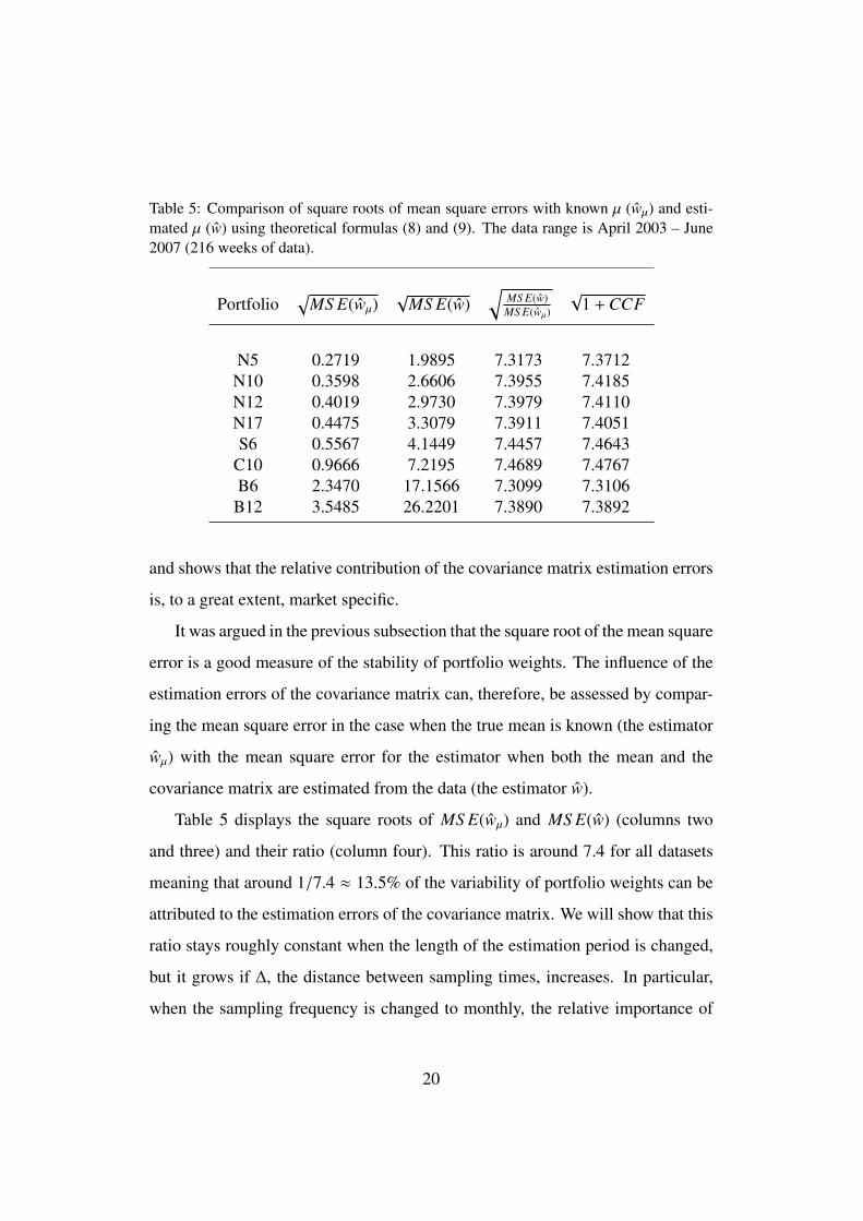
Table 5: Comparison of square roots of mean square errors with known µ (wµ) and esti-

mated µ (w) using theoretical formulas (8) and (9). The data range is April 2003 – June

2007 (216 weeks of data).

Portfolio√

MS E(wµ)√

MS E(w)√

MS E(w)

MS E(wµ)

√1 +CCF

N5 0.2719 1.9895 7.3173 7.3712

N10 0.3598 2.6606 7.3955 7.4185

N12 0.4019 2.9730 7.3979 7.4110

N17 0.4475 3.3079 7.3911 7.4051

S6 0.5567 4.1449 7.4457 7.4643

C10 0.9666 7.2195 7.4689 7.4767

B6 2.3470 17.1566 7.3099 7.3106

B12 3.5485 26.2201 7.3890 7.3892

and shows that the relative contribution of the covariance matrix estimation errors

is, to a great extent, market specific.

It was argued in the previous subsection that the square root of the mean square

error is a good measure of the stability of portfolio weights. The influence of the

estimation errors of the covariance matrix can, therefore, be assessed by compar-

ing the mean square error in the case when the true mean is known (the estimator

wµ) with the mean square error for the estimator when both the mean and the

covariance matrix are estimated from the data (the estimator w).

Table 5 displays the square roots of MS E(wµ) and MS E(w) (columns two

and three) and their ratio (column four). This ratio is around 7.4 for all datasets

meaning that around 1/7.4 ≈ 13.5% of the variability of portfolio weights can be

attributed to the estimation errors of the covariance matrix. We will show that this

ratio stays roughly constant when the length of the estimation period is changed,

but it grows if ∆, the distance between sampling times, increases. In particular,

when the sampling frequency is changed to monthly, the relative importance of

20

covariance estimation errors becomes substantial: the ratio of MSEs lowers to

around 3.5, i.e., 28% of the portfolio weights estimation error is due to the covari-

ance matrix (see Subsection 3.5).

To gain better understanding of the market characteristics determining the de-

gree of the influence of the covariance matrix estimation errors on the stability

of estimated portfolio weights let us return to formulas (5) and (7). Define the

covariance contribution factor as the ratio of the third to the second term of (7):

CCF =( n∆

n − 2µTΣ−1µ

)−1

.

If one assumes that the first term of (5) and (7) is small in comparison to the

other terms (this is very likely as this term is approximately equal to the ratio be-

tween the norm of the market portfolio – bounded by 1 due to the lack of negative

positions – and the number of samples) then

MS E(w) ≈ MS E(wµ)(1 +CCF).

This relation is market-specific. Indeed, the covariance contribution factor can be

written as

CCF =( n∆

n − 2γ2

mwTmΣwm

)−1

=( n∆

n − 2(S Rm)2

)−1

,

where S Rm is the Sharpe ratio of the market portfolio. The relative benefit of

knowing the mean is shared by all mean-variance investors irrespective of their

risk aversion. The driving force in the covariance contribution factor is the Sharpe

ratio of the market portfolio multiplied by ∆, the length of the time interval be-

tween subsequent samples.9 The factor n/(n−2) is close to 1 for practically viable

number of samples n. This implies that varying n results in negligible change in

the balance between the influence of the estimation errors of the mean and the

covariance matrix on the stability of portfolio weights estimator.

9This explains almost identical values in column 5, Table 5, as in our experiment we assumed

Sharpe ratio of market portfolio approximately 1 for all datasets.

21

In general, without the assumption that the first term of (5) and (7) is negligi-

ble, the benefit of knowing the true mean in the optimization process can only be

bounded by the covariance contribution factor CCF:

√MS E(w)√

MS E(wµ)=

√

A + 1 +CCF

A + 1≤√

1 +CCF, (11)

where A > 0 equals the ratio of the first to the second term of (5). The quantity

1/√

1 +CCF underestimates the influence of the covariance matrix estimation

errors on the stability of portfolio weights.

We argued before that the first term of (5) is usually small relative to the other

terms. Hence, the value A in (11) is small and the right-hand side of the inequality

provides a good approximation for the ratio of mean square errors. Indeed, the

last column of Table 5 lists√

1 +CCF for all datasets. These values are in very

good agreement with the exact quantities displayed in column four. This shows

that CCF, which can be easily derived from the properties of the market portfolio,

is a good gauge for the impact of the estimation errors of the covariance matrix on

the stability of estimated portfolio weights.

Portfolio estimation errors diminish its performance. The loss of utility is

examined by Kan and Zhou (2007). Following DeMiguel, Garlappi and Uppal

(2009) we study the turnover. We compute the portfolio turnover by averag-

ing over 100 rolling horizon simulations with weekly rebalancing of portfolio.

There are 200 rebalancing times in which the portfolio is estimated using 216 past

weekly returns. A simulation study spanning a number of datasets and risk aver-

sion coefficients shows that the ratio of square roots of mean square errors has

99% correlation with the ratio of expected turnover implied by strategies com-

puted with the known mean and with the mean estimated from the market data.

22

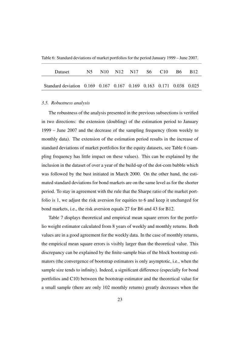
Table 6: Standard deviations of market portfolios for the period January 1999 – June 2007.

Dataset N5 N10 N12 N17 S6 C10 B6 B12

Standard deviation 0.169 0.167 0.167 0.169 0.163 0.171 0.038 0.025

3.5. Robustness analysis

The robustness of the analysis presented in the previous subsections is verified

in two directions: the extension (doubling) of the estimation period to January

1999 – June 2007 and the decrease of the sampling frequency (from weekly to

monthly data). The extension of the estimation period results in the increase of

standard deviations of market portfolios for the equity datasets, see Table 6 (sam-

pling frequency has little impact on these values). This can be explained by the

inclusion in the dataset of over a year of the build-up of the dot-com bubble which

was followed by the bust initiated in March 2000. On the other hand, the esti-

mated standard deviations for bond markets are on the same level as for the shorter

period. To stay in agreement with the rule that the Sharpe ratio of the market port-

folio is 1, we adjust the risk aversion for equities to 6 and keep it unchanged for

bond markets, i.e., the risk aversion equals 27 for B6 and 43 for B12.

Table 7 displays theoretical and empirical mean square errors for the portfo-

lio weight estimator calculated from 8 years of weekly and monthly returns. Both

values are in a good agreement for the weekly data. In the case of monthly returns,

the empirical mean square errors is visibly larger than the theoretical value. This

discrepancy can be explained by the finite-sample bias of the block bootstrap esti-

mators (the convergence of bootstrap estimators is only asymptotic, i.e., when the

sample size tends to infinity). Indeed, a significant difference (especially for bond

portfolios and C10) between the bootstrap estimator and the theoretical value for

a small sample (there are only 102 monthly returns) greatly decreases when the

23

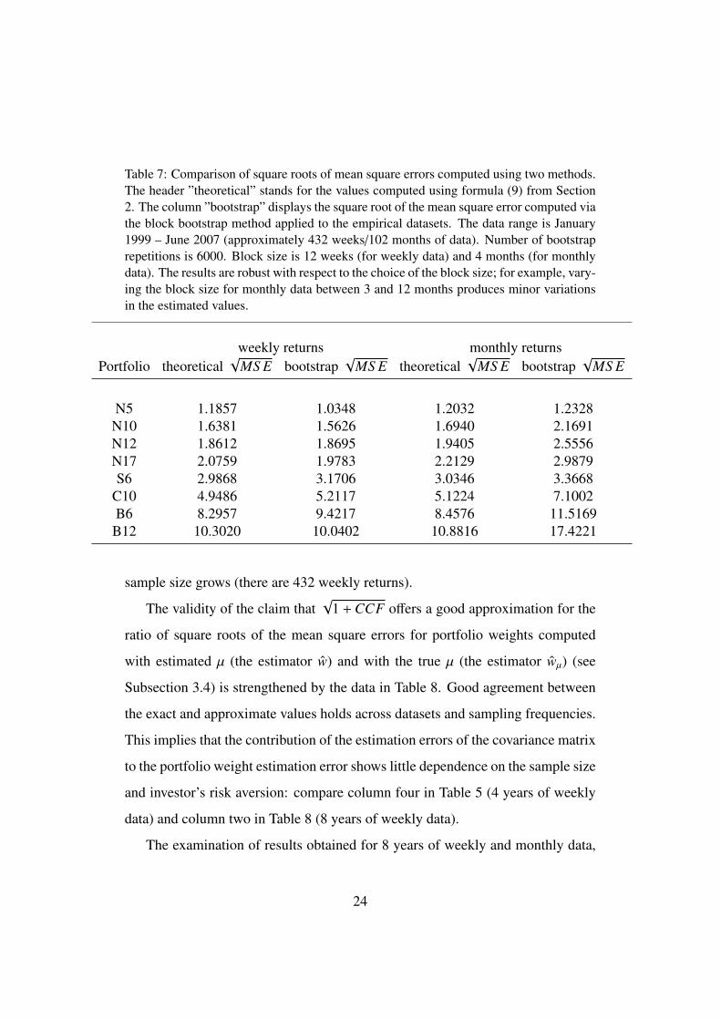
Table 7: Comparison of square roots of mean square errors computed using two methods.

The header ”theoretical” stands for the values computed using formula (9) from Section

2. The column ”bootstrap” displays the square root of the mean square error computed via

the block bootstrap method applied to the empirical datasets. The data range is January

1999 – June 2007 (approximately 432 weeks/102 months of data). Number of bootstrap

repetitions is 6000. Block size is 12 weeks (for weekly data) and 4 months (for monthly

data). The results are robust with respect to the choice of the block size; for example, vary-

ing the block size for monthly data between 3 and 12 months produces minor variations

in the estimated values.

weekly returns monthly returns

Portfolio theoretical√

MS E bootstrap√

MS E theoretical√

MS E bootstrap√

MS E

N5 1.1857 1.0348 1.2032 1.2328

N10 1.6381 1.5626 1.6940 2.1691

N12 1.8612 1.8695 1.9405 2.5556

N17 2.0759 1.9783 2.2129 2.9879

S6 2.9868 3.1706 3.0346 3.3668

C10 4.9486 5.2117 5.1224 7.1002

B6 8.2957 9.4217 8.4576 11.5169

B12 10.3020 10.0402 10.8816 17.4221

sample size grows (there are 432 weekly returns).

The validity of the claim that√

1 +CCF offers a good approximation for the

ratio of square roots of the mean square errors for portfolio weights computed

with estimated µ (the estimator w) and with the true µ (the estimator wµ) (see

Subsection 3.4) is strengthened by the data in Table 8. Good agreement between

the exact and approximate values holds across datasets and sampling frequencies.

This implies that the contribution of the estimation errors of the covariance matrix

to the portfolio weight estimation error shows little dependence on the sample size

and investor’s risk aversion: compare column four in Table 5 (4 years of weekly

data) and column two in Table 8 (8 years of weekly data).

The examination of results obtained for 8 years of weekly and monthly data,

24

Table 8: Comparison of square roots of mean square errors with known µ (wµ) and esti-

mated µ (w) using theoretical formulas (8) and (9). The data range is January 1999 – June

2007 (approximately 432 weeks/102 months of data).

weekly returns monthly returns

Portfolio√

MS E(w)

MS E(wµ)

√1 +CCF

√

MS E(w)

MS E(wµ)

√1 +CCF

N5 7.1140 7.1821 3.5050 3.5370

N10 7.2101 7.2372 3.5497 3.5624

N12 7.2191 7.2340 3.5540 3.5609

N17 7.1490 7.1642 3.5215 3.5287

S6 7.4285 7.4458 3.6508 3.6589

C10 7.0959 7.1027 3.4971 3.5003

B6 7.0208 7.0221 3.4625 3.4631

B12 6.7331 6.7336 3.3299 3.3301

Table 8, reveals that the values for weekly data are approximately twice as large as

the values for monthly data. This fits our theoretical finding that the value of CCF

is inversely proportional to the length of the sampling interval (sampling interval

for monthly data is approximately 4 times larger than for weekly data, hence the

impact of the error coming from the estimation of the covariance matrix is twice

as large as for weekly data). The relative contribution of the estimation errors

of the covariance matrix to the portfolio weight estimation error, i.e., the ratio√

MS E(wµ)/MS E(w), is, therefore, around 28% for monthly data and around

14% for weekly data.

4. Conclusions and further research

We provide analytical formulas linking parameters of the return distribution

with the stability of portfolio weight estimators. Our results are exact, i.e., they

are based on the true, not asymptotic, distributions of the estimators of the mean

and covariance matrix of asset returns. The variability of portfolio weights is

25

measured by the mean square error which combines estimation errors of separate

portfolio weights into a single number. This facilitates the comparison of various

estimation methods and allows for the identification of factors influencing the es-

timation procedure. We show that the relative contribution of estimation errors

of covariance matrix to estimation errors of portfolio weights is market specific

and determined mostly by the Sharpe ratio of the market portfolio and the fre-

quency of asset price sampling. This gives solid grounding for the verification of

the long-standing belief that the covariance matrix related errors are of one order

of magnitude lower than those coming from the estimation of the mean. Our em-

pirical study shows that this is approximately true if the data is sampled weekly

(around 14% of the error is due to the covariance matrix), but is clearly false for

the monthly data (the contribution of covariance related errors grows to 28%).

Our theoretical results are complemented by a thorough study of eight datasets

of equities and bonds with varying sizes. We demonstrate that our theoretically

computed mean square error of the portfolio estimator is in good agreement with

the mean square error estimated from the empirical distribution of the real market

data. The latter was obtained via an appropriate adaptation of the block bootstrap

methodology, which preserves not only the distribution of returns but also their

serial correlation. We believe that this methodology should gain wider popularity

as a tool for assessing properties of portfolio estimators.

Further research could attempt to provide an analysis of portfolio weights esti-

mation error for other settings: Bayesian and shrinkage estimators and the Black-

Litterman model. The extention of our theoretical results to the market model

without riskless asset is straightforward. The mean square error can be derived

from the results of Mori (2004) or Okhrin and Schmid (2006), but the simplifica-

tion of these formulas so that the factors influencing the behavior of the optimal

portfolio estimator can be detected is rather complicated. Our preliminary compu-

26

tations show that the removal of the riskless asset does not provide a remarkable

change of the error. Another line of research could seek to quantify the effect of

growing number of available assets (see Leung, Ng and Wong (2012) and refer-

ences therein) and transaction costs.

Acknowledgments

Financial support from Polish Ministry of Science and Higher Education,

grants [NN-201-547838] and [NN-201-371836], is gratefully acknowledged. We

would also like to thank the anonymous referees for valuable comments.

References

Anderson, T.W. (2003). An Introduction to Multivariate Statistical Analysis, Third

Edition. New York: John Wiley & Sons.

Best, M.J., and R.R. Grauer. (1991a). On the sensitivity of mean-variance-

efficient portfolios to changes in asset means: Some analytical and computational

results. Review of Financial Studies 4: 315–342.

Best, M.J., and R.R. Grauer. (1991b). Sensitivity analysis for mean-variance

portfolio problem. Management Science 37: 980–989.

Best, M.J., and R.R. Grauer. (1992). Positively weighted minimum-variance port-

folios and the structure of asset expected returns. Journal of Financial and Quan-

titative Analysis 27: 513–537.

Bevan, A., and K. Winkelmann. (1998). Using Black-Litterman global asset allo-

cation model: three years of practical experience. Goldman Sachs, Fixed Income

Research, June 1998.

Black, F. (1990). Equilibrium exchange rate hedging. Journal of Finance 45:

899–907.

27

Broadie, M. (1993). Computing efficient frontiers using estimated parameters.

Annals of Operations Research 45: 21–58.

Britten-Jones, M. (1999). The sampling error in estimates of mean-variance effi-

cient portfolio weights. Journal of Finance 54: 655–671.

Chopra, V.K., and W.T. Ziemba. (1993). The effects of errors in the means,

variances, and covariances. Journal of Portfolio Management 19: 6–11.

DeMiguel, V., L. Garlappi, and R. Uppal. (2009). Optimal versus naive diversifi-

cation: How inefficient is the 1/N portfolio strategy? Review of Financial Studies

22: 1915–1953.

Dickinson, J.P. (1974). The reliability of estimation procedures in portfolio anal-

ysis. Journal of Financial and Quantitative Analysis 9: 447–462.

Efron,B., and C. Stein. (1981). The jackknife estimate of variance. Annals of

Statistics 9: 586–596.

Fama, E. (1965). The behavior of stock market prices. Journal of Business 38:

34–105.

Frost, P.A., and J.E. Savarino. (1986). An empirical Bayes approach to efficient

portfolio selection. Journal of Financial and Quantitative Analysis 21: 293–305.

Gentle, J. E., W. K. Hardle, and Y. Mori. (2004). Handbook of Computational

Statistics: Concepts and Methods. Berlin: Springer.

Haff, L.R. (1979). An identity for the Wishart distribution with applications. Jour-

nal of Multivariate Analysis 9: 531–544.

Hall, P., J. L. Horowitz, and B.-Y. Jing. (1995). On blocking rules for the bootstrap

with dependent data. Biometrika 82: 561–574.

Hardle, W., J. Horowitz, and J.-P. Kreiss. (2003). Bootstrap methods for time

series, International Statistical Review 71: 435–459.

28

Hocking, R.R. (2003). Methods and Applications of Linear Models, Second Edi-

tion. New York: John Wiley & Sons.

Jobson, J.D., and B. Korkie. (1980). Estimation of Markowitz efficient portfolios.

Journal of American Statistical Association 75: 544–554.

Jobson, J.D., and B. Korkie. (1989). A performance interpretation of multivariate

tests of asset set intersection, spanning, and mean-variance efficiency. Journal of

Financial and Quantitative Analysis 24: 185–204.

Jorion, P. (1991). Bayesian and CAPM estimators of the means: Implications for

portfolio selection. Journal of Banking and Finance 15: 717–727.

Kan, R., and G. Zhou. (2007). Optimal portfolio choice with parameter uncer-

tainty. Journal of Financial and Quantitative Analysis 42: 621–656.

Leung, P.L., H.Y. Ng, W.K. Wong. (2012). An improved estimation to make

Markowitzs portfolio optimization theory users friendly and estimation accurate

with application on the US stock market investment. European Journal of Opera-

tional Research 222: 85–95.

Litterman, R. (2003). Modern Investment Management: An Equilibrium Ap-

proach. New York: John Wiley & Sons.

McNeil, A.J., R. Frey, and P. Embrechts. (2005). Quantitative Risk Management:

Concepts, Techniques and Tools. Princeton and Oxford: Princeton University

Press.

Markowitz, H. M. (1952). Portfolio selection. Journal of Finance 7: 77–91.

Mori, H. (2004). Finite sample properties of estimators for the optimal portfolio

weight. Journal of Japan Statistical Society 34: 27–46.

Okhrin, Y., and W. Schmid. (2006). Distributional properties of portfolio weights.

Journal of Econometrics 134: 235–256.

29

Pagan, A. (1996). The econometrics of financial markets. Journal of Empirical

Finance 3: 15–102.

30

Electronic supplement

A. Auxiliary statistical theorems

The following statistical results are required in the derivation of closed-form

formulas for the mean-square error (see Theorem B.1).

Theorem A.1. (Haff (1979)[Theorem 3.2]) Assume S follows Wishart distribution

Wp(Σ,N), where p is the dimension of the random square matrix S .

1. ES −1 =1

N − p − 1Σ−1

2. If C is a positive semidefinite p × p matrix

E

S −1CS −1 =1

(N − p)(N − p − 1)(N − p − 3)tr(Σ−1C)Σ−1

+1

(N − p)(N − p − 3)Σ−1CΣ−1.

Lemma A.2. Let X be normally distributed N(m,Ω) and C be a positive semidef-

inite matrix of same dimension as Ω. Then E[XTCX] = mTC m + tr(CΩ).

Proof. Denote by B any square matrix such that C = BT B. Let Y = BX. The

random variable Y has the distribution N(Bm, BΩBT ) and E[XTCX] = E‖Y‖2. The

matrix BΩBT is positive semidefinite. There exists an orthogonal matrix V and a

diagonal matrix Λ, consisting of eigenvalues of BΩBT , such that BΩBT = VTΛV .

Let Z = VY . Then Z has the distribution N(VB m,Λ) and E‖Z‖2 = E‖Y‖2. The

independence of coordinates of Z implies

tr(Λ) = E

(Z − VB m)T (Z − VB m)

.

Trace of a matrix is invariant with respect to the change of basis: tr(BΩBT ) =

tr(Λ). Hence

tr(BΩBT ) = trΛ = EZT Z − 2 E[ZT ]VB m + mT BT VT VB m

= EZT Z − mTC m = E[XTCX] − mTC m.

To complete the proof notice that tr(BΩBT ) = tr(BT BΩ) = tr(CΩ).

1

B. Main theorem

The optimal portfolio weights, i.e., the solution to (1), are given by the follow-

ing formula:

w∗ =1

γΣ−1µ.

An estimator of optimal portfolio weights is constructed using the above formula

with the true µ and Σ replaced by their estimators:

wµ =A

γΣ−1µ, w =

A

γΣ−1µ,

where A is a scaling factor. We assume that µ ∼ N(µ,Σ/(n∆)) and Σ = 1nWp(Σ, n−

1) are independent; n is the size of the sample, ∆ is the distance between sampling

times, and p is the number of risky assets (the dimension of µ), see Section 1.

Theorem B.1. Under the above assumptions, we have

Ewµ =An

n − p − 2w∗, (B.1)

E

‖wµ − w∗‖2

=A2n2

γ2(n − p − 1)(n − p − 2)(n − p − 4)tr(Σ−1)µTΣ−1µ (B.2)

+(

1 +A2n2

(n − p − 1)(n − p − 4)− 2An

n − p − 2

)

‖w∗‖2,

and

Ew = An

n − p − 2w∗, (B.3)

E

‖w − w∗‖2

= E

‖wµ − w∗‖2

(B.4)

+A2n

γ2∆(n − p − 1)(n − p − 4)tr(Σ−1)

(

1 +p

n − p − 2

)

.

Proof. We only prove the second part as the first is simpler and can be done in an

analogous way.

Due to the independence of Σ and µ, we have

Ew = A

γEΣ−1Eµ = A

γ

n

n − p − 2Σ−1µ,

2

where the last equality follows from Theorem A.1. This proves (B.3).

Expand the norm

E

‖w − w∗‖2

= EwT w − 2EwT w∗ + ‖w∗‖2. (B.5)

The first term reads

EwT w = A2

γ2EµT Σ−2µ.

Random variables µ and Σ are independent. Hence,

EµT Σ−2µ = EEµT Σ−2µ|µ = EµTEΣ−2µ.

Theorem A.1 implies

µTEΣ−2µ = n2

(n − p − 1)(n − p − 2)(n − p − 4)tr(Σ−1)µTΣ−1µ

+n2

(n − p − 1)(n − p − 4)µTΣ−2µ.

The expectation of µTΣ−1µ equals EYT Y for Y = Σ−1/2µ with the distribution

N(Σ−1/2µ, 1/(n∆)). By Lemma A.2, EYT Y = µTΣ−1µ + p/(n∆). Similarly,

EµTΣ−2µ = ‖Σ−1µ‖2 + tr(Σ−1)/(n∆) = γ2‖w∗‖2 + tr(Σ−1)/(n∆).

Using (B.3), the second term of (B.5) equals

EwT w∗ = An

n − p − 2‖w∗‖2.

Combing above results gives

E

‖w − w∗‖2

=

=A2

γ2

n2

(n − p − 1)(n − p − 2)(n − p − 4)tr(Σ−1)

(

µTΣ−1µ + p/(n∆))

+A2

γ2

n2

(n − p − 1)(n − p − 4)

(

γ2‖w∗‖2 + tr(Σ−1)/(n∆))

− 2An

n − p − 2‖w∗‖2 + ‖w∗‖2.

3

C. Datasets

N5: Kenneth French’s 5 US Industry Portfolios.

N10: Kenneth French’s 10 US Industry Portfolios.

N12: Kenneth French’s 12 US Industry Portfolios.

N17: Kenneth French’s 17 US Industry Portfolios.

S6: Kenneth French’s 2 × 3 Portfolios Formed on Size and Book-to-Market

(with dividends).

C10: Kenneth French’s 10 Deciles of Portfolios Formed on Size.

The above datasets contain daily total returns for the period from 1 January

1999 until 30 June 2007. Daily excess returns are constructed by subtracting

daily risk-free rate which is also available from Kenneth French’s database.

B6: US government bonds divided into 6 maturity sectors: 1-3 years, 3-5

years, 5-7 years, 7-10 years, 10-15 years and over 15 years (these data are by

courtesy of Merrill Lynch & Co., Inc.). Daily returns for the period from 1 January

1999 until 30 June 2007. Excess returns are constructed from these data using

daily risk free rate calculated from 1M LIBOR (these data are the courtesy of

British Bankers’ Association).

B12: Government bonds of USA, UK and Germany divided into 4 maturity

sectors: 1-3 years, 3-5 years, 5-7 years and 7-10 years (12 instruments: 4 maturity

sectors in 3 currencies) – these data are courtesy of Merrill Lynch & Co., Inc.

Daily returns for the period from 1 January 1999 until 30 June 2007. Fully hedged

excess returns in USD are calculated using historical daily exchange rates taken

from the Bank of England (http://www.bankofengland.co.uk) and risk-free rate in

the corresponding markets obtained from 1M LIBOR (these data are by courtesy

of British Bankers’ Association).

The daily data of excess returns for all above mentioned datasets are cumulated

to weekly excess returns (by compounding returns from Monday to Friday).

4