theoretical calculation of wall - university of north texas
TRANSCRIPT

~th
I N
/Chemistry DivisionChemistry DivisionChemistry DivisionChemistry DivisionChemistry DivisionChemistry Division
7 ANL-87-34
Measuring the AbsoluteDisintegration Rate of aRadioactive Gas with a
Moveable Endplate DischargeCounter (MEP) and
Theoretical Calculation ofWall Effect
William
S0
by Arthur H. Jaffey, James Gray,C. Bentley, and Jerome L. Lerner
Argonne National Laboratory, Argonne, Illinois 60439operated by The University of Chicago
for the United States Department of Energy under Contract W-31-109-Eng-38
Chemistry DivisionChemistry DivisionChemistrv DI)M'i
DISTRIBUTION OF THIS DOCUMENT IS UNLIMITED
Argonne National Laboratory, with facilities in the states of Illinois and Idaho, isowned by the United States government, and operated by The University of Chicagounder the provisions of a contract with the Department of Energy.
DISCLAIMER
This report was prepared as an account of work sponsored by anagency of the United States Government. Neither the UnitedStates Government nor any agency thereof, nor any of theiremployees, makes any warranty, express or implied, or assumesany legal liability or responsibility for the accuracy, com-pleteness, or usefulness of any information, apparatus, product,or process disclosed, or represents that its use would not infringeprivately owned rights. Reference herein to any specific com-mercial product, process, or service by trade name, trademark,manufacturer, or otherwise, does not necessarily constitute orimply its endorsement, recommendation, or favoring by theUnited States Government or any agency thereof. The views andopinions of authors expressed herein do not necessarily state orreflect those of the United States Government or any agencythereof.
Printed in the United States of AmericaAvailable from
National Technical Information ServiceU. S. Department of Commerce5285 Port Royal RoadSpringfield, VA 22161
NTIS price codesPrinted copy: A04Microfiche copy: A01
Distribution Category:Chemistry (UC-4)
ANL-87-34
ARGONNE NATIONAL LABORATORY9700 South Cass Avenue
Argonne, Illinois 60439
ANL--87-34
DE88 001956
MEASURING THE ABSOLUTE DISINTEGRATION RATE OF A RADIOACTIVE GASWITH A MOVEABLE ENDPLATE DISCHARGE COUNTER (MEP)
AND THEORETICAL CALCULATION OF WALL EFFECT
by
William C.Arthur H. Jaf fey, James Gray,Bentley, and Jerome L. Lerner (deceased)
Chemistry Division
Work completed: June 1986
Date Published: September 1987

A major purpose of the Techni-cal Information Center is to providethe broadest dissemination possi-ble of information contained inDOE's Research and DevelopmentReports to business, industry, theacademic community, and federal,state and local governments.
Although a small portion of thisreport is not reproducible, it isbeing made available to expeditethe availability of information on theresearch discussed herein.

I
TABLE OF CONTENTS
1.0 INTRODUCTION AND HISTORY 1
2.0 DESCRIPTION OF MEP 6
2.1 Structure 6
2.2 Mode of Operation 9
2.3 Circuitry 11
2.4 Two Counting Systems 14
3.0 PRECISION FILLING OF MEP 16
3.1 Vacuum Line for Filling 16
3.2 Calibrated Bulbs 17
3,3 Filling Gases. Quench Gas. 17
3.4 Filling Gases. ?krypton Gas 17
3.5 Filling Procedure 19
4.0 OPERATION OF MEP 20
4.1 Placement 20
4.2 Setting Operating Parameters 20
4.3 Some Operating Problems 21
5.0 MEASUREMENTS 22
5.1 Method 22
5.2 Calculation Method. Weighted Least Squares 24
5.3 Alternative Calculation Method. Minimum Chi-Square 24
5.4 Background and "Dead" Krypton 26
5.5 The Gas Fills 27
5.6 Measurement Results 27
5.7 Comparison of Uncorrected (for Wall Effect) Measurement
with the KrI Two-Counter Calibration 31
6.0 ACKNOWLEDGEMENTS 33
REFERENCES 34

ii
APPENDIX A. CALCULATION OF "WALL-EFFECT" IN GM TUBES A-1
1.0 INTRODUCTION A-1
2.0 CALCULATION OF P(B) A-4
2.1 Geometry of the Calculation A-4
2.2 Outline of the Calculation A-4
2.3 Statistical Considerations A-S
2.4 Calculation A-10
2.5 Computer Computation A-14
3.0 DETERMINATION OF P(C) A-17
4.0 COMPUTATION RESULTS A-21
5.0 DISCUSSION A-21
APPENDIX B ON THE 85Kr HALF-LIFE B-1
APPENDIX C ON APPLYING MINIMUM CHI-SQUARE ESTIMATION TO
SPECIFIC ACTIVITY DATA DERIVED FROM POISSON-
DISTRIBUTED MEASUREMENTS C-1
1.0 Gaussian, Poisson, and Chi-Square Distributions C-1
1.1 Gaussian C-1
1.2 Standardized Gaussian C-1
1.3 Chi-Square C-1
1.4 Functions of Gaussian Variables C-2
1.5 Poisson C-3
1.6 Chi-Square with Poisson-based Data C-3
2.0 MINIMUM CHI-SQUARE FOR ESTIMATION C-4
3.0 APPLICATION OF MINIMUM CHI-SQUARE TO EVALUATION OF SPECIFIC
ACTIVITY FROM MEP MEASUREMENTS C-4

iii
LIST OF FIGURES
Page
Fig. 1. Modeling the counter as a large central section withuniform counting rate per cm, with two small end sectionshaving smaller counting rates per cm . . . . . . . . . . .
Fig. 2. Diagram of MEP (Movable Endplate Counter) . . . . . . .
Fig. 3. Measurements with MEP . . . . . . . . . . . . . . . . .
Fig. A-1. Integration volume . . . . . . . . . . . . . . . . . . . .
Fig. A-2A. Beta particle emitted from point Q along path L, which isparallel to the wire . . . . . . . . . . . . . . . . . . .
Fig. A-2B. Beta particle emitted from point Q along path L indirection perpendicular to that in Fig. A-2A . . . . . . .
Fig. A-3. Geometry of calculation . . . . . . . . . . . . . . . . .
Fig. A-4. Emission into d0 interval . . . . . . . . . . . . . . . .
Fig. A-5. Normalized beta spectrum of 85Kr, I(E) vs. E . . . . . .
Fig. A-6. Primary ionization cross section (cm ) as a function of Efor Krypton and Ethyl Ether . . . . . . . . . . . . . . .
Fig. A-7. Relative value of the integrand quantity I(E)/H(E) as afunction of E........ ... . .0.. . . . ....... ..
. 4
7
24
. A-5
A-6
A-6
A-7
. A-ll
A-16
A-18
A-19
iv
LIST OF TABLES
Table 1. MEASURED BULB VOLUMES (ml) 18
Table 2. CHEMICAL COMPOSITION OF 8 5Kr GAS SAMPLE (KrII)
AND "DEAD" KRYPTON (KrIII) 18
Table 3. MEP COUNTING DATA FOR FILL NO. 1 25
Table 4. MEASUREMENTS OF SLOPE BACKGROUND 28
Table 5. PROPERTIES OF VARIOUS GAS FILLS 29
Table 6. SPECIFIC ACTIVITY RESULTS FOR KrII (Uncorrected for Wall Effect) 30
Table 7. SPECIFIC ACTIVITY RESULTS FOR KrII (Corrected for Wall Effect) 32
Table A-1. COMPUTED WALL-EFFECT RESULTS A-2 2

1
MEASURING THE ABSOLUTE DISINTEGRATION RATE OF A RADIOACTIVE GAS
WITH A MOVEABLE END PLATE DISCHARGE COUNTER (ME?)
AND THEORETICAL CALCULATION OF WALL-EFFECT
by
Arthur H. Jaffey, James Gray,
William C. Bentley and Jerome L. Lerner (deceased)
ABSTRACT
A precision built movable endplate Geiger-Muller counter was
used to measure the absolute disintegration rate of a beta-
emitting radioactive gas. A Geiger-Muller counter used for
measuring gaseous radioactivity has <100% counting efficiency
owing to two factors: (1) "end effect", due to decreased and
distorted fields at the ends where wire-insulator joints are
placed, and (2) "wall effect", due to non-ionization by beta-
particles emitted near to and heading into the wall. The end
effect was evaluated by making one end of the counter movable and
measuring counting rates at a number of endplate positions. Much
of the wall effect was calculated theoretically, based on known
data for primary ionization of electrons as a function of energy
and gas composition. Corrections were then made for the
"shakeoff" effect in beta decay and for backscattering of
electrons from the counter wall. Measurements and calculations
were made for a sample of 8 5 Kr (beta energy, 0.67 MeV). The wall
effect calculation is readily extendable to other beta energies.
1.0 INTRODUCTION AND HISTORY
The disintegration rate of a gaseous radioactive substance is
conveniently measured with a gas counter, the radioactivity being mixed with
an appropriate counting gas. This method has a number of advantages, provided
that the chemical nature of the radioactive substance is compatible with the

proper operation of the gas counter. In the majority of cases of interest,
the radioactivity involves the emission of electrons in each decay process,
and the work described here is focused on this type of radioactive species.
The counter often employed in such measurement is a discharge counter in the
form of a cylinder with an axial wire, which is operated either as a
proportional counter or a Geiger-Muller (GM) counter. The use of an internal
counter avoids the problems of solid angle evaluation and correction for
absorption in the counter wall or sample container which arise when the radio-
active sample is measured by placing it external to a counter. If every decay
yields an electron, and if every electron is counted, the disintegration rate
may be derived directly from the counting rate. Most of the emitted electrons
are indeed counted in such an internal counter, so it is a good choice for
disintegration rate determination. We report here on a measurement of the
disintegration rate cf a krypton gas sample containing the radioactive species
85Kr.
In making such a measurement, it has long been known that it is essential
to correct for certain losses that occur in these gas counters which cause the
rate at which discharges occur to be less than the disintegration rate. These
losses are generally described as arising from the end-effect and the wall-
effect. The end-effect causes the more important loss, and results from the
fact that the electric field distribution which creates the countable
discharges is not the same throughout the counter. The radial distribution of
field is longitudinally uniform through a large central region of the counter,
but changes radically near the ends due to the fact that the counter is there
terminated by insulators which support the wire. The discharges created by
ionizing particles near the ends tend to be smaller than those created near
the tube center, and are not counted.
The losses that occur at the tube ends depend considerably on the design
of the insulating region. In the period when gas counters were the
predominant form of radioactivity detector in use, considerable research was
carried out aimed at improving the field distribution at the counter ends.
The gas counter is still quite convenient for measuring gaseous radioactive
samples, and it is only when the actual disintegration rate is to be evaluated
with some accuracy (< 5% error) that end effect losses are carefully
considered.

The wall effect arises because of the stochastic process involved when an
electron loses energy in passing through an absorber, in this case the counter
gas. If the absorber is thin enough, there is some probability that a beta-
particle emitted near the wall will not create any ionization at all before it
hits the wall. As described in the Appendix, the probability of zero ions
formed through ionization by a beta particle of energy E (provided it is not
backscattered) is:
-N i LP(O) = e a p 11]
where
Na = number of gas molecules per cm3
J, = cross section for primary ionization (emission of an electron from a
gas molecule due to collision with a beta particle.)
L = distance (cm) from the point of beta decay ti the tube wall,
measured along the beta particle trajectory.
In order to evaluate the effect accurately, it is necessary to include all the
variations of: (i) beta particle energy E, i.e., beta-particle intensity as a
function of E and sp as a function of E; (ii) position of emission; (iii)
direction of emission; and (iv) distance to wall. The wall effect is
generally of the order of 1% or less in magnitude, and a major part of it can
be calculated from the known physical quantities in the variables (i-iv). An
analysis of the calculation procedure is presented in Appendix A as well as
the results of a particular set of calculations for the radioactive species
and the gas filling discussed in this paper.
The magnitude of the end effect is larger and is not readily
calculable. Correction for the effect, therefore, has generally been carried
out empirically. The basic concept for the experimental evaluation has been
to use two or more cylindrical counters with widely different lengths L1, L2,
L3 ... , but with identical (and uniform) internal diameters, identical wires,
and identical end structures. For example, we consider a case with two
counters (1,2), which are alike in all respects except length.
The first counter (of length L1) may be treated as a large central region
with counting rate per unit length kc with two smaller end regions (of lengths
AA and A.B) with unit counting rates kA and kB (Fig. 1). On the assumption
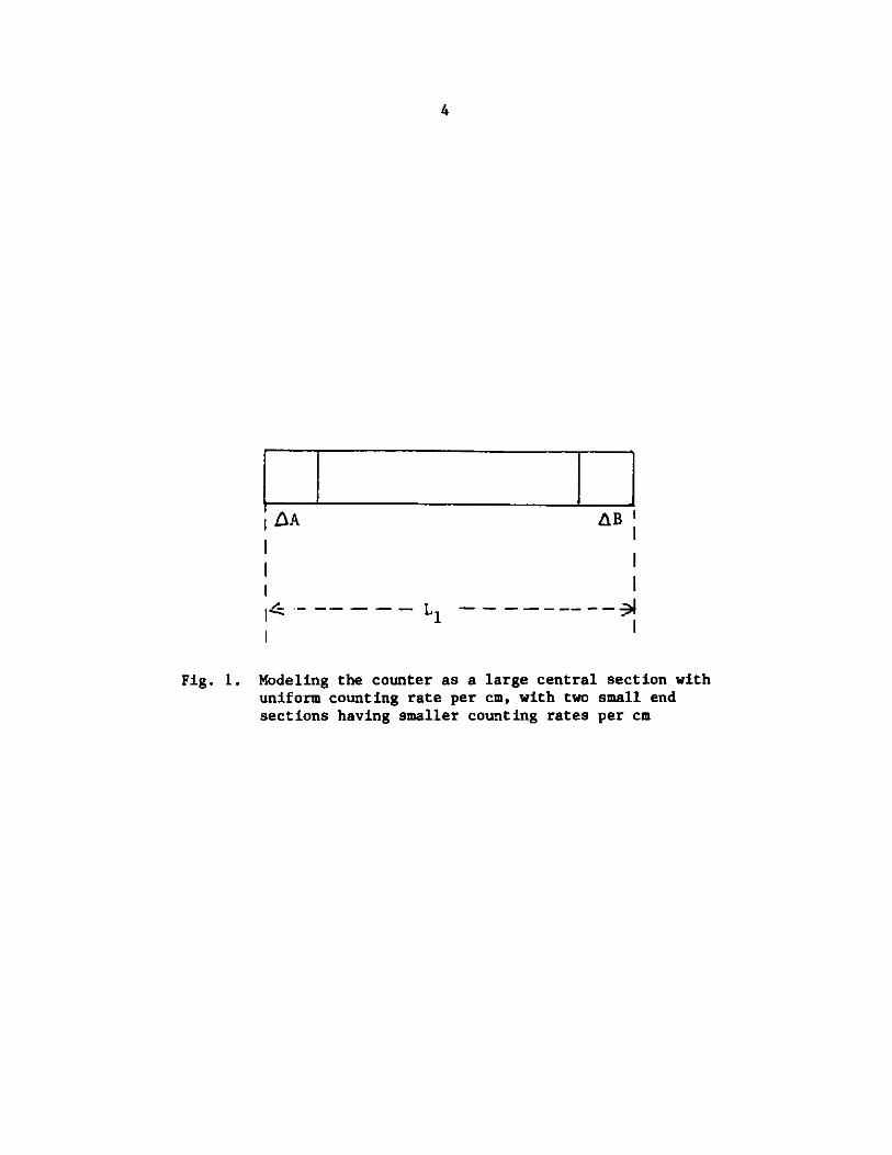
4
AB'1 A
Fig. 1. Modeling the counter as a large central section withuniform counting rate per cm, with two small endsections having smaller counting rates per cm
1 1 1

5
that the counts from the central and end sections may be treated indepen-
dently, the counting rate from this counter is:
C1 - kAAA + kC(L1 -AA - AB) + kB AB [2A]
If the same concentration of radioactive gas is measured in the second counter
(length L2) and if operating conditions (gas pressure and composition,
operating voltage and electronics arrangement) are the same, then
C2 kAAA + kc(L 2 - AA - AB) + kBAB [2B]
Since the counts from the ends are the same in both counters, the difference
in counting rates is:
C-C2 -C-kC(L2 - L1) [2C]
In effect, one has measured the gas in a shorter tube with no end effects.
This method has been used by a number of investigators who wished to
measure the disintegration rate of a radioactive gas. If the concentration of
the radioactive isotope in the total gas is also measured, the technique then
allows the determination of the specific activity (hence, the half-life) of a
long-lived radioactive species such as 14 C. (Typical examples of the two
counter approach are given in Refs. 1-6).
In the 1950's there was considerable work done by French T. ("Pete")
Hagemann at the Argonne National Laboratory (ANL) to develop this technique.
After extensive experiments in which a number of attempts were made to make
identical end structures for the long and short counters, he succeeded in
making some tubes which had end structures which were reasonably closely
alike. Using two sizes of stainless steel counters (3" i.d. x 12" long and 3"
i.d. x 24" long), he measured the absolute disintegration rates of several
kinds of radioactive gas, including a sample of 8 5Kr gas (here denoted as
KrI).
The latter sample was of particular interest to us since some samples of
85Kr have been kept at ANL as long-lived reference gases for calibrating the
counting efficiencies of gas counters. The original two-counter calibration

6
was done in 1954 on KrI, which was later compared to a more active 85Kr gas
sample after KrI had considerably decayed. Comparisons were made by counting
both KrI and its replacement gas in the same GM counters, with no attempt at
absolute disintegration measurement. Hence, only a ratio of disintegration
rates was determined. The original calibration was then periodically
preserved in new 8 5Kr gas samples as they replaced the older ones whenever
these had decayed too much. The current reference gas (KrII), whose absolute
disintegration rate could then be related to that of KrI, was measured in the
present experiment.
After completing this work with the two-counter method, Hagemann was not
satisfied that the counter ends were satisfactorily replicated to the accuracy
he desired, so he attempted an alternative approach involving a single
counter. With the assistance of one of the authors (J.G.) and the machinist
Thomas Fallon, he tied a number of designs of moveable piston counters. In
such a counter, the wire was fastened to a feedthrough insulator in a fixed
position at one end and was strung through the center of a moveable insulating
piston at the other end. A necessary feature of the design was that the
counter should produce measurable pulses only on one side of this piston. The
effective length of the counter could then be varied, and since the end
structures (insulator feedthrough and piston) remained the same at each
length, measurements corresponded to those in counters of different lengths
with identical end effects.
A satisfactory design was developed by 1957; it was called the MEP
(Moveable End-Plate) counter. Shortly after a few preliminary measurements
were made, Hagemann became ill, and further work with MEP ceased. It was set
aside in storage and it was not until recently that it was decided to carry
out some definitive measurements with MEP to demonstrate that it could,
indeed, be used for accurate measurement of disintegration rates. Measurement
of the current reference 85Kr gas (KrII) would allow comparison of MEP results
with the previous two-counter measurement of KrI.
Other work using moveable end counters has been described in Refs. 8-10.
2.0 DESCRIPTION OF MEP
2.1 Structure. Diagrammatic drawings of the essential elements of MEP
are shown in Fig. 2. The body of the counter is a heavy wall (~5 mm

Fixed Vernier
MoveableScale
BellowsShaft
Filling PortGold Gaskets
Scale Valve
f--Gold Plated SS Wire
Moveable QuartzEnd Plate End Plates Teflon
(Identical) Insulator
ViP Take up reel
Bellows Shaft
Pinion Gear''-'
Quartz
ContactingGoldFeedt hrough
Fig. 2. Diagram of MEP (Movable Endplate Counter)
16 v -W mw - w v 0 mw w or

8
thickness) tube of OFHC copper ~48 cm long and with an outside diameter of
~6 cm. Flanges for use of gold "0-rings" are attached to the ends. The
mating flange at one end holds the stationary end of the counter and the
emergent counter wire; at the other end, the mating flange holds the moveable
piston and the precision scale. The interior of the tube was bored and reamed
to complete circularity and straightness, and honed to a shiny surface.
Measurement down the bore showed the tube to be accurately circular and the
diameter to be very uniform, most of the values varying between 1.9944" to
1.9945" (opening up to 1.9946" near the ends). The diameter is taken to be
1.9945" (- 5.066 cm).
The endplates (Fig. 2) at both ends are identical. Each endplate is
essentially a quartz disk held at its outer edge in a brass cylinder which
provides support and serves as the moveable element at one end. A small gold
bushing is set at the center of the disk with a highly polished hole at its
center which is just large enough to allow the wire to slip through. As the
wire passes through the hole, it is slightly offset to insure rubbing contact
with the bushing. This serves to terminate the active wire length at the
position of the disk; some such provision is necessary because the counting
gas is actually present on both sides of each disk.
Back of the moveable quartz disk is a spring loaded rewind mechanism
which coils the wire up as the piston is moved and keeps the wire in the
counting chamber under tension. A quartz cup (not shown in the figure) which
is platinized in its interior surrounds the take-up reel (Fig. 2). The metal
structure of the take-up reel is connected to the platinized surface with a
phosphor bronze spring. Hence, the coiled section of wire is surrounded by
conducting surfaces which are at the same potential. as the wire, thus
preventing the occurrence of counter discharges in regions outside of the
designated counting volume.
The piston is attached to a square rod which has a precision scale on one
face and a fine-tooth rack on the opposite face. The vacuum-tight super-
structure contains a fixed vernier scale, a quartz viewing window, a rotary
bellows vacuum seal with a pinion gear to drive the rack, and a long thin tube
to accommodate the rod with its scale. The accuracy of the etched lines on
the scale was shop-measured with a traveling microscope and found to be at
least as good as 0.01 mm, which is better than the reading achievable with the

9
installed vernier. A magnifying glass and focused light external to the
viewing window allows ready examination of scale and vernier.
Assembly of MEP had to be carried out very carefully. After any
necessary repairs or changes were made, fresh gold gaskets were inserted if
necessary, and all the components (including the wire) and the interior were
washed with fresh, very high purity methyl alcohol. The most difficult part
of the assembly involved mounting the wire. This involved threading it
through the piston and connecting it to the take-up reel, and then passing the
other end through the stationary insulator and soldering it. Final assembly
was followed by pumpout and leak checking.
Relative positions of the moveable endplate could be accurately measured
by observing the position of the rule; displacement of the endplate could be
measured as accurately as the rule could be read. For some purposes, it was
desirable to know the actual length L of the tube portion between the two
endplates. A measurement of L was carefully made with the unit disassembled
and appropriately supported, and the rule position was then set. However, the
actual value of L at a particular rule position setting depended upon the
positions of the two end flanges, and these positions were slightly dependent
upon how much the two gold gaskets were crushed. Since the counter was
disassembled and reassembled many times, the absolute value of L was known
with less accuracy than were the relative displacements of the moveable
endplate.
2.2 Mode of Operation. MEP was found to be usable both as a
proportional counter and as a GM counter, although the wire diameter wa
smaller for the former. For the present measurement, it was decided to use
the GM mode, and the counter was fitted with a 0.003" (0.075 mm) soft temper
stainless steel wire; the alloy was one which allowed the coil to be tightly
coiled up many times without becoming distorted. Using the GM 'mode offered
the advantage that when an ionization event occurs within the cylindrical
electric field, the output pulse size is not dependent (at least in the
central region) on the amount of initial ionization, hence is not a function
of electron energy.
A problem arising with the GM mode is that with some gas fills it was
evident that spurious pulses occasionally formed which occurred shortly after
true ionization events. When the spurious pulses occurred, they were detected
10
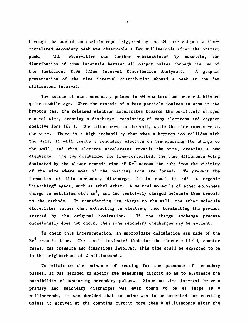
through the use of an oscilloscope triggered by the GM tube output; a time-
correlated secondary peak was observable a few milliseconds after the primary
peak. This observation was further substantiated by measuring the
distribution of time intervals between all output pulses through the use of
the instrument TIDA (Time Interval Distribution Analyzer). A graphic
presentation of the time interval distribution showed a peak at the few
millisecond interval.
The source of such secondary pulses in GM counters had been established
quite a while ago. When the transit of a beta particle ionizes an atom in the
krypton gas, the released electron accelerates towards the positively charged
central wire, creating a discharge, consisting of many electrons and krypton
positive ions (Kr+). The latter move to the wall, while the electrons move to
the wire. There is a high probability that when a krypton ion collides with
the wall, it will create a secondary electron on transferring its charge to
the wall, and this electron accelerates towards the wire, creating a new
discharge. The two discharges are time-correlated, the time difference being
dominated by the slower transit time of Kr+ across the tube from the vicinity
of the wire where most of the positive ions are formed. To prevent the
formation of this secondary discharge, it is usual to add an organic
"quenching" agent, such as ethyl ether. A neutral molecule of ether exchanges
charge on collision with Kr+, and the positively charged molecule then travels
to the cathode. On transferring its charge to the wall, the ether molecule
dissociates rather than extracting an electron, thus terminating the process
started by the original ionization. If the charge exchange process
occasionally does not occur, then some secondary discharges may be evident.
To check this interpretation, an approximate calculation was made of the
Kr+ transit time. The result indicated that for the electric field, counter
gases, gas pressure and dimensions involved, this time would be expected to be
in the neighborhood of 2 milliseconds.
To eliminate the nuisance of testing for the presence of secondary
pulses, it was decided to modify the measuring circuit so as to eliminate the
possibility of measuring secondary pulses. Since no time interval between
primary and secondary discharges was ever found to be as large as 4
milliseconds, it was decided that no pulse was to be accepted for counting
unless it arrived at the counting circuit more than 4 milliseconds after the

11
previous discharge. This requirement also served the purpose of preventing
the counting of a spurious discharge which was generated secondarily from a
secondary discharge, since this could occur more than 4 milliseconds after the
last count. Thus, the effective deadtime was not a fixed one, but was
extended by 4 milliseconds whenever a discharge occurred less than 4
milliseconds after the last discharge. Since the deadtime could then be
variable, depending upon the rate of spurious discharges, it was necessary to
use a standard livetimer. This measured the total time during which the
counter was available to produce a countable discharge after the last count.
2.3 Circuitry. MEP was operated with the wall at ground potential and
with positive high voltage applied to the center wire through a two megohm
resistor. Pecause of limited space in the shielding tomb, the only circuitry
used there was a line driver (capacitatively coupled to the center wire),
which provided a low impedance signal for the external circuitry. Similarly,
the outputs of the anticoincidence scintillator bank photomultipliers were
delivered by line drivers to the external circuitry.
The scintillator signal was amplified and passed through a pulse height
discriminator to eliminate pulses which were too small to have come from
muons. The surviving pulses triggered a monostable multivibrator (MMV1),
which delivered a 100 us square wave output for use in implementing the
anticoincidence operation discussed below. MMV1 pulses were also accumulated
in the ACB (anticoincidence bank) scaler.
The MEP driver was connected to two independent circuit trains to allow
use of the extending deadtime operation as referred to above as well as a
conventional fixed deadtime. Thus, for fixed deadtime, the driver output
passed through a discriminator, and surviving pulses triggered the
multivibrator MMV2 , with output pulse width 4 ms. This MMV was not retrig-
gerable until the end of the 4 ms period. Immediately after MMV2 fired,
another multivibrator (MMV3) also fired, with a 50 us pulse-width output. The
relative pulse timing was arranged so that the scintillator MMV1 output and
the MEP MMV 3 output overlapped adequately if the initiating events were time-
coincident. The MMV3 output sent enabling signals to two different
multivibrators, MMV4 and MMV5. MMV4 was the BC (before coincidence) unit and
always fired when activated by MMV2. It served to drive the BC scaler,
totaling all acceptable discharges from MEP. MMV5, the AC (after coincidence)

12
unit was also connected to the MMV1 output, and fired only if a scintillation
output pulse was not time-coincident with a MEP MMV3 output pulse. MMV5 drove
the AC scaler, totaling all acceptable MEP discharges which were not time-
coincident with muon scintillations. Then (BC - AC), the difference between
the two scaler outputs was equal to the number of coincidence events between
MEP counts and muon events.
For the extending deadtime system, the circuit train was identical,
except that the discriminator fired a 4 ms MMV which could be retriggered
before the termination of the 4 ms period, and then remained triggered for
only another 4 ms, unless retriggered again. The other components, equivalent
to MMV3 , MMV4 , and MMV5 , and the BC and AC scalers, were identical to those in
the other system. The AC MMV unit for the extending deadtime train was also
used to provide pulses whose time interval distribution was measured with
TIDA.
Each of the two deadtime systems had two timers. One was an elapsed
timer, which was basically a scaler which accumulated a train of 100
pulses/min derived from the 60 cycle power line.* The other was a livetimer,
which also accumulated signals from a train of 100 pulses/min derived from the
60 cycle line. However, this pulse train was interrupted by an anticoincident
system during the time periods that MMV1 or MMV2 (or its extending deadtime
equivalent) were active. Thus, these time periods were not sampled, because
no activation of MMV5 (AC output) could occur while these circuits were
operating. Since the livetimer sampled only "open" time periods, calculation
of the counting rate did not require knowledge of the magnitude of the actual
deadtime.
TIDA, the Time Interval Distribution Analyzer, was a circuit designed to
measure the distribution of time interval lengths between adjacent output
pulses from a radiation detector. Aside from deadtime effects, a normally
operating detector should deliver a train of pulses following a Poisson
process. The distribution of interval lengths from such a process is
exponential.
*Measurements against time standards had shown this time source to be quite
accurate, at least over periods which are a good part of a day, as in thepresent experiment.

13
TIDA was a multichannel time analyzer with time channel boundaries
adjusted on a logarithmic scale. With such an adjustment a Poisson process
should yield (on the average) a uniform distribution over the various
channels. Such uniformity could be perturbed by: (1) the usual fluctuations
expected in any random process, (2) the fact that since TIDA is based on a
digital countdown system, the logarithmic relation could only be approximated
by the sequence of digital numbers chosen for the several channels, and (3)
the deviation of the setting chosen for the countdown rate from that suitable
for the actual mean counting process rate.
In the particular realization of the TIDA design used, an integer
sequence was selected for the various channels, corresponding (with the
necessary digital approximations) to 1% probability from the exponential
distribution in each of the first 8 channels, and 4% probability in each of
the last 23 channels, the final channel having a terminal boundary
corresponding to "infinite" time. In operation, the occurrence of a count
from the counting process train activated a sequence of events: The first
channel integer was entered into a countdown scaler, which was counted down
using an oscillator-driven pulse train of rate F. When the scaler reached
zero, the second channel integer was entered, etc. When the next count from
the counting process train occurred, this advancing process stopped, and a
count was accumulated in the appropriate channel of a standard multichannel
analyzer (MCA). Simultaneously, the first integer was again entered into the
countdown channel, and the sequence advanced until the next counting process
count terminated the countdown. The output consisted of the accumulated
events in the MCA, which represented the distribution of the time-interval
lengths in the counting process.
The frequency F of the oscillator was adjusted so that its rate
corresponded to the mean rate M of the counting process, which had been
evaluated with a short preliminary measurement. The desired ratio of F to M
(i.e., scale factor) was fixed by the particular set of integers stored for
use in the countdown process. If the desired ratio of F to M differed from
the actual one, this would correspond to the various time channels actually
used not being the a priori defined probability (1% and 4% bins). However,
this deviation was correctable in subsequent computer analysis, in a program
which made the necessary adjustments for deviations of the frequency used from

14
the desired value and for the integer approximations to the defined
probability boundaries. Chi-square analysis and graphical presentation served
to give summary results.
2.4 Two Counting Systems. Although the counting rates used were low
enough so that the deadtime corrections were always modest in size, it was
desirable to check the method used by independent procedures. The basic
hardware elements have been described in the Section 2.3 Circuitry.
System 1.. Input with fixed deadtime (initial MMV not
retriggerable), a BC scaler with total output N8 1, an AC scaler
with total output NAL, an elapsed timer with total output TiE and
a livetimer with total output TLL. The measured counting rate
could be calculated in two ways, first by using the livetime value
TLL, or by using the elapsed time TiE and correcting for the
effect of a fixed deadtime with the standard formula for a Type I
counter. A GM tube with an intrinsic deadtime* smaller than the
"clamping" external electronic deadtime is known to be well-fitted
with the Type I relation if the counting rate is not high.
For the first method, the measured counting rate was
C NM[3A]1 T1L
For the second method, the counting rate corrected for deadtime
was:
CAC- = AC (3B]1C 1-T71 CBC 2 CMu
where
CAC - and CBC - [3C]T1E BC T1E
*Intrinsic deadtime as opposed to an externally-applied deadtime created by
electronic circuitry, e.g., a monostable multivibrator. Intrinsic deadtimeis a period following the onset of a discharge during which a new ionizationevent cannot create a new discharge because the traveling positive ionsdistort the counter's electric field.

15
CAC was the observed net counting rate to be corrected for dead-
time losses, but CBC was the rate at which MEP causes deadtimes to
occur. CMu was the muon counting rate (in the scintillator bank)
of those muons which independently caused deadtime periods because
they were not coincident with MEP counts. T1 was the 4 ms
deadtime created by MEP's MMV2 and T2 was the 100 is deadtime
created by the scintillation bank's MMV1. Cu was calculated from
NACB1 (the muon total count in the anticoincidence scintillator
bank) after subtracting the number of events in which muon counts
and MEP counts were coincident. Then
C -NACB1 (NBC NAC[3D]Mu T1E
Since the livetimer was inactivated whenever either the anti-
coincidence bank or MEP delivered an outVut, then
T La TE E-TNB T 2 [NACB1 - (NB1 - NA1) [3E]
Since C1 may be written as
NAL /T1EC 1 - TN /T - T [N - (N -N )]/T1 Bi 1E 2[ACB - BC AC 1E
NAl
TIE TNB1 T2 [NACB1 (NBC NAC [3
it is evident (from Eq. [3E]) that Eq. [3F] is identical to Eq.
[3A]. Hence, calculating the counting rate with either method is
algebraically the same, provided that the livetimer has performed
correctly, and that MEP, at the counting rates used, behaved like
a Type I counter. If secondary spurious events occurred, then
they were counted, and neither C1 nor C applied, since NAL was
inflated by the "false" counts.
System 2. Input with extending deadtime. This system had
the fixed deadtime T 1 of System 1 if none of the dead periods were
extended during the initial 4 ms, s, that either calculation
method could be used for this system, yielding rate C2 and C2 from

16
relations equivalent to Eq. [3A] and Eq. [3B]. However, if an
appreciable number of extended deadtime periods occur, then only
the equivalent of Eq. [3A] was appropriate, and was correct even
when spurious secondary ionization events occurred, since these
were suppressed.
Measuring with the two procedures provided a check for the possible
occurrence of counts from secondary pulses. Although the values actually used
in the experiment were those derived from System 2 and calculated as C2
(extending deadtime with livetimer), the results C1, Cj, C2, and C were all
very close in value. Another check was made by comparing the value of T2L
calculated from Eq. [3E] with the electronically measured value. If the
deadtimes were appreciably extended, then the values calculated from Eq. [3E]
should not agree with the measured livetime, nor should the two livetimer
results TLL and T2L agree. When discrepancies were observed in either the
livetime or counting rate results, the measurements were investigated as
described in Section 4.3 Some Operating Problems.
3.0 PRECISION FILLING OF MEP
It had been established in preliminary measurements that ethyl ether was
a good quenching agent for MEP. The amount of 8 5Kr activity (KrII) to use was
selected as a compromise between the opposing criteria of: (a) adequate
counting rate for achieving the desired total rumber of counts at the extreme
piston position of closest approach, and (b) avoiding too much deadtime at the
other extreme (wide open) piston position. In an attempt to evaluate the wall
effect experimentally, measurements were made at various krypton pressures.
The same amount of KrII was used in each fill, and the krypton pressure was
varied by changing the amount of added "dead" krypton gas which had a small,
though non-zero, disintegration rate.
3.1 Vacuum Line for Filling. To minimize potential gas contamination by
adsorbed gases, the filling was carried out in a vacuum line constructed
entirely of stainless steel tubing and valves except for the calibrated
volumes, which were pyrex bulbs. A gas pressure, p, could be measured with a
precision quartz-bourdon gauge accurate to the relative error 0.06% at p - 100
Torr, smaller relative errors at p > 100 Torr, and an absolute error of 0.05
Torr for p < 100 Torr (Ruska Digital Pressure Gauge, DDR-6000).

17
3.2 Calibrated Bulbs. Attached to the manifold with shut-off metal
valves were a number of glass bulbs of various volumes which were used to
prepare defined gas mixtures for MEP. The volume of each bulb was calibrated
by first evacuating it and then filling it with pure xenon gas (<0.05%
impurity) to a measured pressure (approximately 1 atm) and finally freezing
the gas quantitatively into a preweighed and evacuated small, strong stainless
steel vessel cooled to liquid nitrogen temperature. After warming, the steel
vessel was weighed again with a semimicro balance, the gain in weight
corresponding to the xenon previously contained in the bulb. A water bath
surrounding the bulb was used to control the xenon gas temperature, which was
measured to better than 0.2*C (0.07% accuracy). The weight gain, xenon
temperature, and pressure sufficed to give the bulb volume, using the value of
xenon density as 5.2527 g/1 at 740 Torr, 25 C. This method of measuring the
standard volumes is described in Ref. 7.
Each bulb was calibrated several times; the average values are shown in
Table 1 (error indicated is standard error of the mean). The results in the
table indicate that our goal of <0.1% error was satisfied. Each of the flasks
#1 and #2 was designed to be a mixing chamber to homogenize the mixtures
prepared. Each had a long freeze-down finger at the bottom which could be
cooled with liquid or solid nitrogen to allow condensation of gases from the
other flasks on the manifold.
3.3 Filling Gases. wench Gas. The ethyl ether was ibaken from a fresh
unopened container of "absolute ether". The purification process was designed
to remove traces of water and oxygen. The water was removed by mixing the
ether with Linde molecular sieve #4 which had been activated by heating under
vacuum. After three days of drying, the ether-sieve mix was cooled with
liquid nitrogen and pumped. It was then warmed up and the ether transferred
to the storage bulb by distillation and cryogenic cooling. Final traces of
oxygen were removed by about eight stages of freezing the ether with liquid
nitrogen and pumping it. The process was complete when the vacuum gauge
showed no pressure over the frozen ether.
3.4 Filling Gases. Krypton Gas. KrII, the krypton gas supply
containing 85Kr, and the "dead" krypton supply (KrIII) were analyzed mass
spectrometrically and found to have the compositions given in Table 2. The
nominally "dead" KrIII was used for diluting the specific activity of KrII.

18
Volume
MEASURED
Flask
Table 1
BULB VOLUMES (ml)
Volume Flask Volume
#1 1057.44 t 0.10 A 151.45 t 0.11 C 219.99 t 0.08
#2 1075.88 0.03 B 215.96 f 0.01 D 229.47 t 0.03
Table 2
CHEMICAL COMPOSITION OF 8 5 Kr GAS SAMPLE (KrII)
AND "DEAD" KRYPTON (KrIII)
Percent
Species
Kr
H2
He
H20N2
CO
02
Ar
C02
Other
KrII
> 99.89
< .05
.02
< .04
< .003
.002
N.D.*
KrIII
>99.8
< .07
< ,01
.02
< .03
< .003
.06
< .006
N.D.*
*N.D. - Not detected.
Flask

19
It actually had a slight amount of activity which had to be accounted for in
calculating the results. This was measured in ordinary cylindrical GM
counters whose counting efficiencies were calibrated with KrII. KrIII
specific activity was measured as 0.0131 dpm/ml (at adopted conditions, 760
Torr, 25 C), as of June 1, 1983.
3.5 Filling Procedure. The amount of KrII to be used in the counting
gas mixture was fixed by the counting rate desired. This was chosen to be
about 1000 cpm when the piston was pulled all the way out, a compromise
between a rate which would yield too much deadtime and a rate which would
yield an adequate number of counts in a reasonable time.
The gas mixture was prepared by introducing pre-calculated pressures of
the three component; ethyl ether, KrII and KrIII into separate calibrated
bulbs, and then transferring two of the components into the third bulb (either
Flask #1 or Flask #2), where all three components were mixed. Since the
mixture could not be transferred quantitatively from the mixing bulb into MEP,
it was necessary to prepare more mixture than needed for MEP, allowing for the
gas necessarily to be left in the manifold and the mixing bulb. Thus the
ratio*
R Vol. (mixing bulb) + Vol. (manifold) + vol. (MEP)vol Vol. (MEP)
was measured by entering some gas into MEP at a measured pressure Pi, closing
the valve to MEP, pumping out the manifold and mixing bulb, opening the MEP
valve, and measuring the final pressure P2. Since Rvol = P1 /2, the pressure
of gas in the mixing bulb needed to fill MEP to a desired pressure Pd was
readily determined. When Flask #2 was used as the mixing bulb, Rvol = 2.365,
so that the mixing bulb was filled to an initial pressure (2. 3 6 5 )Pd'
Two of the smaller flasks and a "one liter" flask were attached to the
manifold and thermostated in the water bath. Then the desired amount of ether
was transferred to one of the small flasks and the pressure precisely
measured; this was chosen so that the ether pressure constituted a specified
percentage (often 10%) of the total fill pressure. After clearing the
*The MEP volume included the active counting volume as well as the "dead"
volumes on the outside of both insulator discs, including the extensionvolume containing the precision rule.

20
manifold, a defined pressure of KrII was entered into the other small flask
and measured in the same way, KrIII was placed into the one liter flask, say
Flask #2. After the manifold was pumped out, the pressure gauge was shut off,
all three flasks opened to the manifold and liquid nitrogen placed around the
freezedown finger of Flask #2. Solidifying the nitrogen by pumping on it
condenses the ether and all krypton into the cold finger. After pressure
measurement with the gauge indicated the residual pressure to be <0.01 mm,
Flask #2 was isolated from the manifold.
Mixing the gases was carried out by setting up convection currents
through heating the freezedown finger and cooling the top of Flask #2. After
thermal equilibrium was reestablished, the gas was expanded into the evacuated
and air-thermostated MEP. The gas pressure was measured and the MEP body
temperature was measured at three points with platinum thermometers; readings
agreed to <0.2*C.
4.OOPERATION OF MEP
4.1 Placement. MEP was mounted within a tomb shield with 8 inches of
steel wall and inside an anticoincidence counter made of slabs of 2 inch thick
solid plastic scintillator surrounding the counter space. The tomb, when
closed, acted as an effective air thermostat; the temperature at various
points of MEP, as measured with several Pt thermometers, was uniform to
<0.2C.
The scintillator anticoincidence shield served to decrease background
from very penetrating particles muonss). A muon passing through MEP would
also pass through the plastic shield, resulting in an ionization discharge
within MEP and a light pulse in the scintillator. Photomultipliers placed
around the edges of the scintillator 'labs picked up the light pulse, and a
triggered anticoincidence circuit suppressed the counting of the MEP discharge
which was time-coincident with this pulse. The total counting rate (KrII +
muon) determined the total deadtime of the counting system, the muon rate
being about 20% of that of KrII.
4.2 SettingjOperating Parameters. Rather than measuring plateau
characteristics, a tedious procedure, a suitable high voltage was determined
by measuring the pulse height distribution from MEP. As the high voltage was
increased, attainment of the Geiger region was indicated by the fact that the
21
pulse heights became essentially uniform. The operating point was then
selected to be 25 to 50 volts higher. The actual voltage used depended upon
the ethyl ether and krypton pressures, going up when either was increased.
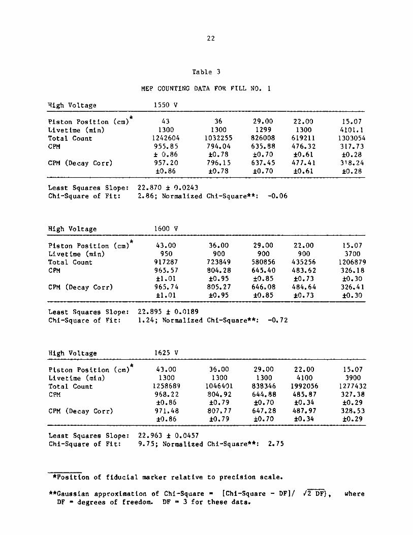
Typical values are shown in Table 3. At a constant high voltage value,
measurements were made at five positions of the piston, at precision scale
readings 43, 36, 29, 22, and 15 cm.
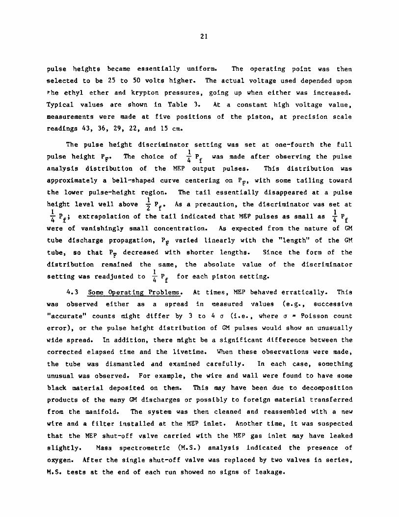
The pulse height discriminator setting was set at one-fourth the full1
pulse height PF. The choice of 4 P was made after observing the pulse
analysis distribution of the MEP output pulses. This distribution was
approximately a bell-shaped curve centering on PF, with some tailing toward
the lower pulse-height region. The tail essentially disappeared at a pulse1
height level well above 7 Pf . As a precaution, the discriminator was set at1 14 Pf; extrapolation of the tail indicated that MEP pulses as small as - P
were of vanishingly small concentration. As expected from the nature of GM
tube discharge propagation, PF varied linearly with the "length" of the GM
tube, so that PF decreased with shorter lengths. Since the form of the
distribution remained the same, the absolute value of the discriminator1
setting was readjusted to - P for each piston setting.
4.3 Some Operating Problems. At times, MEP behaved erratically. This
was observed either as a spread in measured values (e.g., successive
"accurate" counts might differ by 3 to 4 a (i.e., where a - Poisson count
error), or the pulse height distribution of GM pulses would show an unusually
wide spread. In addition, there might be a significant difference between the
corrected elapsed time and the livetime. When these observations were made,
the tube was dismantled and examined carefully. In each case, something
unusual was observed. For example, the wire and wall were found to have some
black material deposited on them. This may have been due to decomposition
products of the many GM discharges or possibly to foreign material transferred
from the manifold. The system was then cleaned and reassembled with a new
wire and a filter installed at the MEP inlet. Another time, it was suspected
that the MEP shut-off valve carried with the MEP gas inlet may have leaked
slightly. Mass spectrometric (M.S.) analysis indicated the presence of
oxygen. After the single shut-off valve was replaced by two valves in series,
M.S. tests at the end of each run showed no signs of leakage.
22
Table 3
MEP COUNTING DATA FOR FILL NO. 1
High Voltage 1550 V
Piston Position (cm)* 43 36 29.00 22.00 15.07Livetime (min) 1300 1300 1299 1300 4101.1Total Count 1242604 1032255 826008 619211 1303054CPM 955.85 794.04 635.88 476.32 317.73
0.86 0.78 0.70 0.61 0.28CPM (Decay Corr) 957.20 796.15 637.45 477.41 31.8.24
0.86 0.78 0.70 0.61 0.28
Least Squares Slope: 22.870 0.0243Chi-Square of Fit: 2.86; Normalized Chi-Square**: -0.06
High Voltage 1600 V
Piston Position (cm)* 43.00 36.00 29.00 22.00 15.07Livetime (min) 950 900 900 900 3700Total Count 917287 723849 580856 435256 1206879CPM 965.57 804.28 645.40 483.62 326.18
1.01 0.95 0.85 0.73 0.30CPM (Decay Corr) 965.74 805.27 646.08 484.64 326.41
1.01 0.95 0.85 0.73 0.30
Least Squares Slope: 22.895 0.0189Chi-Square of Fit: 1.24; Normalized Chi-Square**: -0.72
High Voltage 1625 V
Piston Position (cm)* 43.00 36.00 29.00 22.00 15.07Livetime (min) 1300 1300 1300 4100 3900Total Count 1258689 1046401 838346 1992056 1277432CPM 968.22 804.92 644.88 485.87 327.38
0.86 0.79 0.70 0.34 0.29CPM (Decay Corr) 971.48 807.77 647.28 487.97 328.53
0.86 0.79 0.70 0.34 0.29
Least Squares Slope:Chi-Square of Fit:
22.963 0.04579.75; Normalized Chi-Square**: 2.75
*Position of fiducial marker relative to precision scale.
**Gaussian approximation of Chi-Square - [Chi-Square - DFI/DF - degrees of freedom. DF - 3 for these data.
/2 DF}, where

23
At another disassembly, small bends were found on the center wire. It
was hypothesized that this might have been due to crossover of the wire on the
take-up reel. After a small spiral groove was machined on the reel surface as
a guide for the wire, this problem did not recur.
5.0 MEASUREMENTS
5.1 Method. Since plateau plots (count rate vs. high voltage) had
slopes of the order of ~1% per 100 V, it was not appropriate to use a single
voltage operating point. Instead, measurement was made of counting rate vs.
piston position at several high voltage values for which the output pulse
distribution was single peaked. At any particular voltage setting, a plot of
these data yielded a straight line, as expected, and the slope value was
calculated by weighted least squares. The slope represented an estimate of
the disintegration rate of a gas volume at the center of MEP consisting of a
cylindrical slab 1 cm high and with the MEP radius. The same procedure was
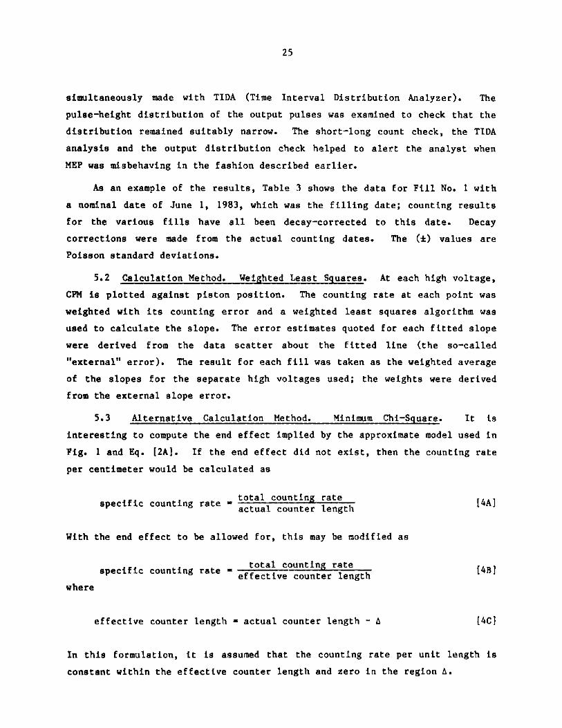
used for several high voltage values, and the slopes were averaged. Fig. 3
illustrates the experimental results for one particular gas mixture. Although
the counting rate at a particular piston position increased a little with the
high voltage value, the slope was the same at the several voltages.
The standard reference conditions used were: pressure, 760 Torr;
temperature, 25*C; date, June 1, 1983. Since measurements were made over a
period of a year, the 8 5 Kr decay was corrected to the reference date, using
the value T1/2 - 10.75 yr (see Appendix B).
After a particular mixture was placed in MEP and the operating voltage
selected, counting was carried on at this voltage at five piston positions,
mostly separated by 7 cm, i.e., at rule readings 43, 36, 29, 22, and 15.46 or
15.55 cm. The last interval was constrained by the limits of available
movement. For some measurements, calculation was carried out by slightly
extrapolating the "15 cm" measurement to 15.00. In other measurements, the
actual position was used in the calculation. MEP was counted at each piston
position for one day; 300 minutes during the working day and 1000 minutes
overnight. Because its counting rate was least, the "15 cm" position was left
for Friday, so that it gave a 300 minute count and an approximately 3800
minute count over the weekend. The short and long counts were checked for
consistency and then averaged. Time interval distribution measurements were

24
41...... 'i' J ' 11: .. .i'' .:V:. :V
COUNT RATE . . - . . . . ..... ...... .. , . . . ... . . . . . .. . . . .. . .. .. .. . . . . . .... .... " .'..:: . .... .e :.::R . .. 4. ". " . .1.I ... . ee Tit! :1 ee e e l :t: . t g. . .. ::.: . :. e .. .. .. . ee.. 1;
...... .... :. . . . . . . . ... .... m ~~ eeee.e 4e,... me-..s .-. e -.... :...... .:. ... ..: . .. .":: .b.ar .. 6 w . " :. "". .. . " ":: e e e me e e e ... ."" .1 . ": . .. .. . "r." ."... t"
7 7777~
.....
...
i 1 &vh t it...
900
800
700
600
500
400
300214
CM I
30 314 40 42 44
..K ... . . ...
Fig. 3. Measurements with MEP
Lines fitted to data of counting rate vs. relative pistonposition for Gas Fill No. 1. (Data in Table 3.)
SLOPES: SA = 22.87 Ct. Rate per Cm
SB = 22.90
SC = 22.99
GAS FILL No. 1: Partial Pressure (standard conditions)KrII = 20.18 mi, Ether = 7.51%Total Pressure = 201.8 mm
HIGH VOLTAGE: A 1550 V
B 1600 V
C 1625 V
16 20
. :,"
-. "----
i
i
.H.
25
simultaneously made with TIDA (Time Interval Distribution Analyzer). The
pulse-height distribution of the output pulses was examined to check that the
distribution remained suitably narrow. The short-long count check, the TIDA
analysis and the output distribution check helped to alert the analyst when
MEP was misbehaving in the fashion described earlier.
As an example of the results, Table 3 shows the data for Fill No. 1 with
a nominal date of June 1, 1983, which was the filling date; counting results
for the various fills have all been decay-corrected to this date. Decay
corrections were made from the actual counting dates. The (t) values are
Poisson standard deviations.
5.2 Calculation Method. Weighted Least Squares. At each high voltage,
CPM is plotted against piston position. The counting rate at each point was
weighted with its counting error and a weighted least squares algorithm was
used to calculate the slope. The error estimates quoted for each fitted slope
were derived from the data scatter about the fitted line (the so-called
"external" error). The result for each fill was taken as the weighted average
of the slopes for the separate high voltages used; the weights were derived
from the external slope error.
5.3 Alternative Calculation Method. Minimum Chi-Square. It is
interesting to compute the end effect implied by the approximate model used in
Fig. 1 and Eq. [2A]. If the end effect did not exist, then the counting rate
per centimeter would be calculated as
specficcoutin rae -total counting ratespecificounting rate = actual counter length [4A]
With the end effect to be allowed for, this may be modified as
specific counting rate total countngLratLe4 B]effective counter lengthwhere
effective counter length - actual counter length - A [4C]
In this formulation, it is assumed that the counting rate per unit length is
constant within the effective counter length and zero in the region A.

26
The evaluation of A is not possible with only one value of actual counter
length, but the joint results of counting with several lengths can yield an
estimate of A, provided we assume that A is the same for all counter
lengths -- the basic assumption of our measurement. It is shown in Appendix C
how this may be most efficiently carried out with the nonlinear estimation
process of minimum chi-square.
Details of the calculation results are omitted, since the resulting
values of counting rate per unit length (from Eqn. [4B]) are identical to
those derived from the weighted least squares estimates given in Table 6. An
interesting sidelight derived from the calculations indicates that A decreases
with increasing high voltage. If the specific counting rate is to be
independent of high voltage, such a variation is necessary, since in a GM tube
voltage plateau, the total counting rate does increase slowly with the high
voltage value (see Eqn. [4B]). One may interpret this increased rate to be
due to the more effective penetration of the electric field into the end
region (at higher voltage), which increases the likelihood of forming
countable pulses. In the approximate model, this shortens the length of the
"dead" region A.
5.4 Background and "Dead" Krypton. Contributing to the counting rate of
KrII in MEP were the counts arising from the background and from the added
diluent "dead" krypton (KrIII). The counting rate of each varied with the
piston position.
As mentioned above, ordinary GM tubes with counting efficiency calibrated
with KrII were used to measure the specific activity of KrIII as 0.0131 (t8%)
dpm/ml (at 760 Torr, 25 C) as of June 1, 1983. Since the slope was
essentially the disintegration rate of an MEP cylindrical section 1 cm high
and of MEP radius, the contribution to a measured slope arising from the KrIII
portion of a fill mixture was calculable from the specific activity, pressure,
and temperature of the added KrIII.
To evaluate the effect of background on the slope measurement, some fills
were made with KrEII and ether and with argon and ether. For the former, the
background was taken as the residual after subtracting the expected low
specific activity effect. Since argon contains no activity, its measured
slope could be taken as the background effect. The two methods gave
essentially the same result, which checks the apriori assumption that the

27
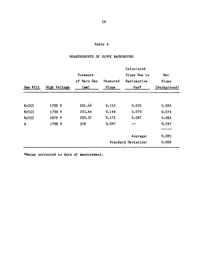
background slope was not affected by the nature of the gas filling. Table 4
gives data for some measurements of the background.
5.5 The Gas Fills. The various gas mixtures (fills) are listed in Table
5. Since the MEP radius is 5.066/2 cm, the counter volume for 1 cm length is
20.1567 cm3. The krypton volume (760 Torr, 250C) contained in this length is
V(Kr) = 20 67 p(Kr) = 0.02652 p(Kr)
where p(Kr) is the krypton pressure (Torr) referred to 25*C.
5.6 Measurement Results. The data and final values for each fill are
given in Table 6. The unweighted average specific activity (as of June 1,
1983) was measured to be
Uncorrected S.A. - 42.152 0.093 dpm/ml
where the error indicated is the standard error of the mean. Then
(error ) x 100 = 0.22%average
This value has not been corrected for the small wall effect, whose magnitude
is calculated in Appendix A.
As shown in this appendix, the wall effect magnitude is proportional to
1/p, where p is the gas pressure. It was originally intended that the wall
effect would be determined empirically through measurements made at several
values of p. A plot of "apparent specific activity" vs 1/p would then yield
an intercept (at p = c) which would yield the wall effect. However, the
behavior of MEP as a GM tube deteriorated with increasing p, so this approach
was abandoned, apparently requiring considerable further study to develop
stable operating conditions.
This kind of empirical approach had also been tried by several other
investigators (Ref. 4,5,6,8,9) either by using the varied-p approach or by
varying counter diameters at -onstant length. The radioactivities measured
had low energy betas: 3H, Emax = 18.6 kev; 35S, Emax = 167 kev; 14C, Emax =
156 key. Results from several experiments showed that for these isotopes, the
wall effect was not observable, within their experimental errors. From the
28
Table 4
MEASUREMENTS OF SLOPE BACKGROUND
Gas Fill High Voltage
Pressure
of Rare Gas
(mm)
Measured
Slope
Calculated
Slope Due to
Radioactive
Gas*
201.44
201.44
250.37
258
0.153
0.146
0.172
0.097
Average:
Standard Deviation:
*Decay corrected to date of measurement.
Net
Slope
(Background)
KrIII
KrIII
KrIII
A
1700 V
1750 V
1875 V
1700 V
0.070
0.070
0.087
0.083
0.076
0.085
0.097
0.085
0.009

Table 5
PROPERTIES OF VARIOUS GAS FILLS
V2ml/cm(b,c)
0.5352
0.5389
0.5450
0.5352
0.5424
0.5487
0.5418
0.5400
0.5302
0.5318
V3ml/cm(b,d)
4.416
4.413
4.497
6.269
4.340
7.457
7.238
7.218
4.241
4.831
Species)Act.KrIIIdpm/ml
0.0131
0.0129
0.0128
0.0128
0.0125
0.0124
0.0124
0.0124
0.0122
0.0122
dpm of Gas Fill dueto 1 cm of 1rIIIAs of At Count6/1/83 Time
0.058
0.058
0.059
0.082
0.057
0.098
0.095
0.095
0.056
0.063
(a) Percent by
(b) Volume (atradius.
pressure.
standard conditions) contained in slyt of MEP: Cylindrical section 1 cm high and with MEP
V2 = Vol (KrII).
V3 = Vol (KrlII).
At standard conditions, 760 n, 25*C.
FillNo. Date
TotalGasPress.(25 C)
201.84
201.84
205.48
277.40
204.51
335.41
325.93
324.99
199.90
224.70
1
2
3
4
5
6
7
8
9
10
PercentKrI I
(a)
10.00%
10.07
10.00
7.223
10.00
6.169
6.267
6.264
10.00
8.923
6/1/83
9/12/83
10/10/83
10/26/83
3/1/84
3/19/84
4/6/84
4/26/84
6/20/84
7/6/84
Press.of KrII(mm)(25 C)
20.18
20. 32
20.55
20.18
20.45
20.69
20.43
20.36
19.99
20.05
PercentKrIII
(a)
82.49%
82.43
82.51
85.21
80.004
83.829
83.734
83.738
80.00
81.068
Press.of KrIII(mm)(25*C)
166.50
166.38
169.54
236.38
163.62
281.17
272.91
272.14
159.92
182.16
0.058
0.057
0.058
0.080
0.054
0.093
0.090
0.089
0.052
0.059
(c)
(d)
(e)
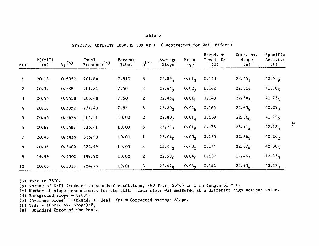
Table 6
SPECIFIC ACTIVITY RESULTS FOR KrII (Uncorrected for Wall Effect)
TotalV2 (b) Pressure(a)
0.5352
0.5389
0.5450
0.5352
0.5424
0.5487
0.5418
0.5400
0.5302
0.5318
201.84
201.84
205.48
277.40
204. 51
335.41
325.93
324.99
199.90
224.70
PercentEther
7.51%
7.50
7.50
7.51
10.00
10.00
10.00
10.00
10.00
10.01
Bkgnd.Average Error "Dead"
n(c) Slope (g) (d)
3
2
2
3
2
3
1
2
2
3
22.894
22.649
22.888
22.803
22.807
23.292
23.04o
23.052
22.596
22.678
0.013
0.023
0.011
0.026
0.018
0.018
0.052
0.030
0.040
0.042
0.143
0.142
0. 143
0. 165
0.139
0. 178
0.175
0.174
0.137
0.144
Torr at 25*C.Volume of KrII (reduced to standard conditions, 760 Torr, 250C) in 1 cm length of MEP.
Number of slope measurements for the fill. Each slope was measured at a different high voltage value.
Background slope = 0.085.(Average Slope) - (Bkgnd. + "dead" Kr) = Corrected Average Slope.S.A. = (Corr. Av. Slope)/V 2
Standard Error of the Mean.
FillP(Kr II)
(a)
+
KrCorr. Av.
Slope
(e)
SpecificActivity
(f)
1
2
3
4
5
6
7
8
9
10
20.18
20.32
20.55
20.18
20.45
20.69
20.43
20.36
19.99
20.05
22.751
22.507
22.745
22.638
22.668
23. 114
22.865
22.878
22.462
22.534
42. 509
41.765
41.734
42.298
41.792
42.125
42.202
42.366
42.359
42.373
LA.
(a)(b)(c)(d)(e)(f)(g)

31
discussion in Appendix A, such a low result would be expected, since, as is
evident from Equation [1], the probability for no ionization in a path length
L is very small if ap is large, which is the case for low energy electrons.
The wall-effect calculations in Appendix A gave values which indicated
that efficiency factors varied from 0.9967 to 0.9942 depending upon the fill
pressure. The specific activity results of Table 6 are corrected for these
wall effect values in Table 7. The corrected specific activity (as of June 1,
1983) is then
Corrected S.A. - 42.347 0.098
This is an unweighted average and the indicated error is the standard error of
the mean.
5.7 Comparison of Uncorrected (for Wall Effect) Measurement with the KrI
Two-Counter Calibration. As discussed earlier, the two-counter value used for
the KrII specific activity was ultimately based upon the KrI two-counter 1954
calibration, through several intermediate ratio comparisons. At each compari-
son, the specific activity of the current standard was decay-corrected with
the then accepted best value for the 85Kr half-life. The value used was
10.70 yr between January 1, 1954 and January 1, 1969 and then 10.76 yr to the
fiducial date June 1, 1983. The decay corrections have been recalculated for
these periods using the currently preferred value of 10.75 yr (Appendix B).
This correction resulted in only a modest change in the presumed value of KrII
at June 1, 1983, namely, approximately 0.73%. The corrected result was 42.04,
slightly larger than the hitherto presumed value of 41.88 dpm/ml. This
quantity was also uncorrected for the wall effect. The original measurement
data for the 2-counter calibration was no longer available, so that no error
could be assigned to the data scatter contribution to the error in the 42.04
value. However, from Appendix B, it is evident that the assigned error in the
8 5Kr half-life value results in another contribution to the error in the 42.04
value since a 8 5Kr decay correction was made from January 1, 1954 to June 1,
1983; the one sigma error contribution is 0.35%.
The MEP and two-counter results are considerably closer than might have
been expected. Thus
42.15Uncorrected MEP Value 2 - 1.002
2-Counter Value 42.04 1 7

32
Table 7
SPECIFIC ACTIVITY RESULTS FOR KrII (Corrected for Wall Effect)
Total
Pressure(a)
201.84
201.84
205.48
277.40
204.51
335.41
325.93
324.99
199.90
224.70
Percent
Ether
7.51%
7.50
7.50
7.51
10.00
10.00
10.00
10.00
10.00
10.01
Uncorrected
Specific
Activity
42.509
41.765
41.734
42.298
41.792
42.125
42.202
42.366
42.359
42.373
Corrected(c)
Specific
Activity
0.0058
0.0058
0.0057
0.0042
0.0054
0.0033
0.0034
0.0034
0.0056
0.0050
42.757
42.009
41.973
42.477
41.930
42.264
42.346
42.510
42.598
42.586
Torr at 25*CProbability of no ionization from 8 5KrA).[Uncorrected Specific Activity]/[1-P0].
beta-particles (Table A, Appendix
Fill
1
2
3
4
5
6
7
8
9
10
(a)(b)
(c)
p (b)

33
For the wall-effect corrected result,42.34
Corrected MEP Value 5= 1.00732-Counter Value 42.04
6.0 ACKNOWLEDGEMENTS
We wish to thank a number of our colleagues for invaluable aid; they are:
THOMAS FALLON, a machinist who had worked with Pete Hagemann in developing MEPand who ably carried out the difficult operation of disassembly,rewiring, and reassembly of MEP,
STANLEY RYMAS, who designed the stainless steel vacuum line used for fillingMEP, and aided in the filling process,
JOHN HUGHES, who constructed the calibration bulbs and the calibration portionof the filling line, and purified the ethyl ether used as quench gas,
MITIO INOKUTI, of the Radiological and Environmental Research Division (ANL),who provided us with the information on cross sections for primaryionization used in Appendix A,
ANTHONY TURKEVICH, (Professor Chemistry, University of Chicago), who providedus with valuable advice,
MELVIN FREEDMAN, (ANL) who provided us with thg5 basic information on theshakeoff effect, and on the beta spectrum of Kr.

34
REFERENCES
1. A. G. Engelkemeir and W. F. Libby, "End and Wall Corrections for Absolute
Beta Counting in Gas Counters", Rev. Sci. Instr. 21, 550-554 (1950).
2. W. B. Mann, T. H. Seliger, W. F. Marlow and R. W. Medlock, "Recalibration
of the NBS Carbon-14 Standard by Geiger-Muller and Proportional Gas
Counting", Rev. Sci. Instr. 31, 690-696 (1960).
3. S. B. Garfinkel, W. B. Mann, F. J. Schima and M. P. Unterweger, "Present
Status in the Field of Internal Gas Counting", Nucl. Instrum. Meth. 112,
59-67 (1973).
4. W. F. Merritt and R. C. Hawkings, "The Absolute Assay of Sulfur-35 by
Internal Gas Counting", Anal. Chem. 32, 308-310 (1960).
5. D. E. Watt, D. Ramsden and H. W. Wilson, "The Half-life of Carbon-14",
Int. J. Appl. Rad Isotopes 11, 68-74 (1961).
6. A. Spernol and B. Denecke, "Prazise Absolutmessung Der AktivitAt von
Tritium. III", J. Appl. Rad. Isotopes 15, 241-254 (1964).
6a. James Gray, Unpublished
7. W. M. Rutherford, "Volumetric Calibration of Experimental Apparatus by
Xenon Gas Transfer", Rev. Sci. Instrum. 49, 1415-1417 (1978).
8. D. Modes and M. Leistner, "Extrapolationszahlrohr zur Absolutbestimmung
von 1'C", Atomkernenergie 6, 363-365 (1961).
9. I. U. Olsson, I. Karlen, A. H. Turnbull and N. J. D. Prosser, "A
Determination of the Half-life of C14 with a Proportional Counter", Ark.
f. Fysik 22, 237-255 (1962).
10. F. Bella, M. Alessio and P. Fratelli, "A Determination of the Half-life
of 14 C", I Nuovo Cimento 588, 233-246 (1968).
11. M. S. Freedman, Private communication.
12. F. F. Rieke and W. Prepejchal, "Ionization of Gaseous Atoms and Molecules
for High-Energy Electrons and Positrons", Phys. Rev. A 6, 1507-1519
(1972). (Written and calculated by M. Inokuti).
13. M. Inokuti, "Inelastic Collisions of Fast Charged Particles with Atoms
and Molecules - The Bethe Theory Revisited", Rev. Mod. Phys. 43, 297-347
(1971). [Fig. 18].
14. H. J. Grosse and H. K. Bothe, "Die Ionisierungs-querschnitte von
Kohlenwasserstoffen und deren Sauerstoffderivaten", Z. Naturforsch 23A
1583-90 (1968).

35
15. Ellis P. Steinberg, "Counting Methods for the Assay of Radioactive
Samples", Chap. 5 of Nuclear Instruments and Their Uses, Ed. Arthur H.
Snell (Wiley, NY, 1962).
16. L. Yaffe and K. M. Justus, "Back-scattering of Electrons into Geiger-
Muller Counters", J. Chem. Soc. S72, 341-351 (Supplement, 1949).
17. H. H. Seliger, "The Backscattering of Positrons and Electrons", Phys.
Rev. 88, 408-412 (1952).
18. Kevin Flynn, (Private communication).
19. M. Inokuti, (Private communication).
20. M. S. Freedman, "Atomic Structure Effects in Nuclear Events", Ann. Rev.
Nucl. Sci. 24, 209-247 (1974).
21. T. A. Carlson, C. W. Nestor, Jr. , Thomas C. Tucker and F. B. Malik,
"Calculation of Electron Shake-off for Elements from Z = 2 to 92 with the
Use of Self-Consistent-Field Wave Functions", Phys. Rev. 169, 27-36
(1968).
22. J. Lerner, "Half-life of 8 5 Kr", J. Inorg. Nucl. Chem. 25, 749-57 (1963).
23. S. C. Anspach, L. M. Cavallo, S. B. Garfinkel, J. M. R. Hutchinson, and
C. N. Smith, private communication to Nuclear Data Group (Jan. 1968);
Nucl. Data Sheets, 5 (2), 131 (1971).
24. James W. Johnston, "Statistical Analysis of a Determination of the Half-
life of Krypton-85", Batelle Northwest Report, BNWL-B-369, (July, 1974).
25. Maurice G. Kendall and Alan Stuart, The Advanced Theory of Statistics,
Vols. 1 and 2. (Griffin, London, 1958 and 1961).

36
A-1
APPENDIX A
CALCULATION OF "WALL-EFFECT" IN GM TUBES
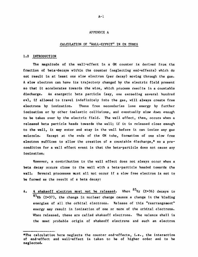
1.0 INTRODUCTION
The magnitude of the wall-effect in a GM counter is derived from the
fraction of beta-decays within the counter (neglecting end-effects) which do
not result in at least one slow electron (per decay) moving through the gas.
A slow electron can have its trajectory changed by the electric field present
so that it accelerates towards the wire, which process results in a countable
discharge. An energetic beta particle (say, one exceeding several hundred
ev), if allowed to travel indefinitely into the gas, will always create free
electrons by ionization. These free secondaries lose energy by further
ionization or by other inelastic collisions, and eventually slow down enough
to be taken over by the electric field. The wall effect, then, occurs when a
released beta particle heads towards the wall; if it is released close enough
to the wall, it may enter and stay in the wall before it can ionize any gas
molecule. Except at the ends of the GM tube, formation of one slow free
electron suffices to allow the creation of a countable discharge,* so a pre-
condition for a wall effect event is that the beta-particle does not cause any
ionization.
However, a contribution to the wall effect does not always occur when a
beta decay occurs close to the wall with a beta-particle headed towards the
wall. Several processes must all not occur if a slow free electron is not to
be formed as the result of a beta decay:
A. A shakeoff electron mst not be released. When 85Kr (Z=36) decays to8 5Rb (Z-37), the change in nuclear charge causes a change in the binding
energies of all the orbital electrons. Release of this "rearrangement"
energy may result in ionization of one or more of the orbital electrons.
When released, these are called shakeoff electrons. The valence shell is
the most probable origin of shakeoff electrons and such an electron
*The calculation here neglects the counter end-effects, i.e., the interaction
of end-effect and wall-effect is taken to be of higher order and to beneglected.

A- 2
generally has a very low energy, of the order of a few ev, hence will
almost certainly result in a counter discharge. Even shakeoff electrons
from inner shells have energies (<20 kev) much lower than the average
beta-particle energy, hence have very high cross sections for ionization,
and will almost certainly cause a discharge. The probability of creating
shakeoff electrons is the same for every decay event and does not depend
upon the beta-particle energy, since the transition energy is the same
for each decay.
B. The decay electron must not create any ionization. Since the maximum
energy of a secondary ionization electron is about one-half the beta-
particle energy, and the energy distribution of the secondaries rises at
least as steeply as 1/Esecat the low energy end,19 a secondary electron,
if formed, is most probably of low energy and almost certainly creates a
discharge. As discussed below, it will be evident that only quite
energetic beta-particles have a low probability of creating an ionization
in the path lengths of significance.
C. The decay electron must penetrate into the wall and must not back-
scatter. If it does backscatter, its trajectory will have a long path-
length in the gas and it will almost certainly create ionization.
A quantitative examination of these processes offers an approach to
estimation of the non-counting probability Po. Thus,
P= =A PI [A-1A]
where PA is the probability of a decay without shakeoff and P is the
probability that a beta-particle will not ionize on the way to the wall and
will not backscatter (processes (B) and (C)).
The calculation of P(B), the probability of process (B), can be carried
out in a straightforward manner, since the function involved have been
measured (or calculated) and are available in published material. In
analyzing this process, one takes into account the random distribution of the
source point in the gas volume, the random distribution of 0 the angle of
emission, the random distribution of E, the energy of the beta-particle
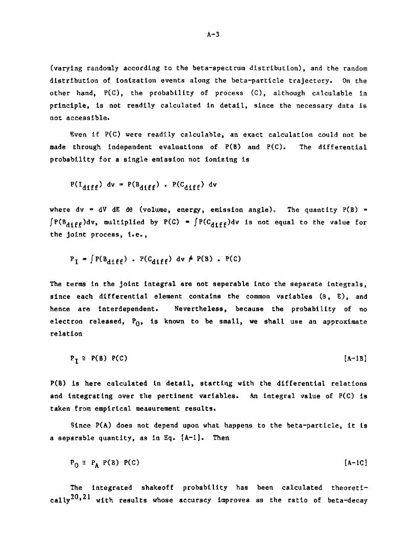
A-3
(varying randomly according to the beta-spectrum distribution), and the random
distribution of ionization events along the beta-particle trajectory. On the
other hand, P(C), the probability of process (C), although calculable in
principle, is not readily calculated in detail, since the necessary data is
not accessible.
Even if P(C) were readily calculable, an exact calculation could not be
made through independent evaluations of P(B) and P(C). The differential
probability for a single emission not ionizing is
P(Idiff) dv = P(Bdiff) * P(Cdiff) dv
where dv a dV dE dO (volume, energy, emission angle). The quantity P(B) =
fP(Bdiff)dv, multiplied by P(C) = fP(Cdiff)dv is not equal to the value for
the joint process, i.e.,
P - JP(Bdiff) P(Cdiff) dv ' P(B) . P(C)
The terms in the joint integral are not seperable into the separate integrals,
since each differential element contains the common variables (0, E), and
hence are interdependent. Nevertheless, because the probability of no
electron released, PO, is known to be small, we shall use an approximate
relation
PI1 = P(B) P(C) [A-1B]
P(B) is here calculated in detail, starting with the differential relations
and integrating over the pertinent variables. An integral value of P(C) is
taken from empirical measurement results.
Since P(A) does not depend upon what happens to the beta-particle, it is
a separable quantity, as in Eq. [A-1]. Then
PO = A P(B) P(C) [A-1C]
The integrated shakeoff probability has been calculated theoreti-
cally2 0'2 1 with results whose accuracy improves as the ratio of beta-decay
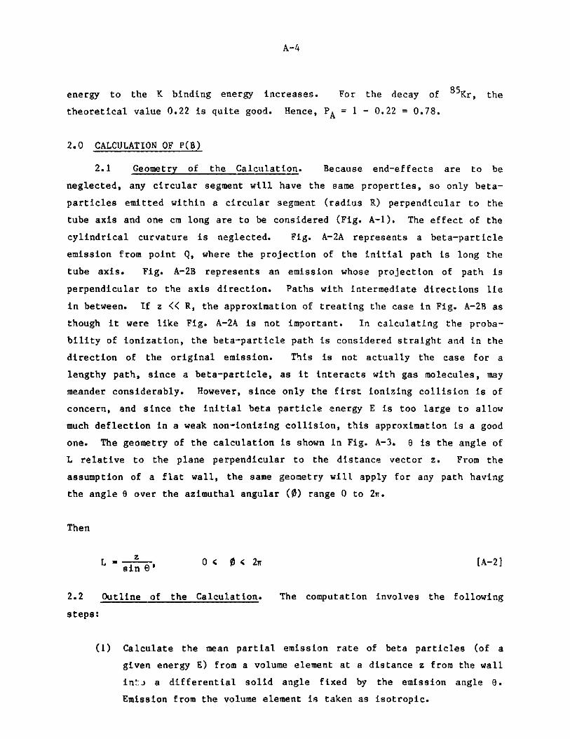
A-4
energy to the K binding energy increases. For the decay of 85Kr, the
theoretical value 0.22 is quite good. Hence, PA = 1 - 0.22 = 0.78.
2.0 CALCULATION OF P(B)
2.1 Geometry of the Calculation. Because end-effects are to be
neglected, any circular segment will have the same properties, so only beta-
particles emitted within a circular segment (radius R) perpendicular to the
tube axis and one cm long are to be considered (Fig. A-1). The effect of the
cylindrical curvature is neglected. Fig. A-2A represents a beta-particle
emission from point Q, where the projection of the initial path is long the
tube axis. Fig. A-2B represents an emission whose projection of path is
perpendicular to the axis direction. Paths with intermediate directions lie
in between. If z << R, the approximation of treating the case in Fig. A-2B as
though it were like Fig. A-2A is not important. In calculating the proba-
bility of ionization, the beta-particle path is considered straight and in the
direction of the original emission. This is not actually the case for a
lengthy path, since a beta-particle, as it interacts with gas molecules, may
meander considerably. However, since only the first ionizing collision is of
concern, and since the initial beta particle energy E is too large to allow
much deflection in a weak non-ionizing collision, this approximation is a good
one. The geometry of the calculation is shown in Fig. A-3. 6 is the angle of
L relative to the plane perpendicular to the distance vector z. From the
assumption of a flat wall, the same geometry will apply for any path having
the angle 0 over the azimuthal angular (0) range 0 to 2 .
Then
L Z '0 < < 2t [A-2]
2.2 Outline of the Calculation. The computation involves the following
steps:
(1) Calculate the mean partial emission rate of beta particles (of a
given energy E) from a volume element at a distance z from the wall
inti a differential solid angle fixed by the emission angle 0.
Emission from the volume element is taken as isotropic.

A- 5
Fig. A-1. Integration Volume. Cylindrical box made ofcircular segmet perpendicular to the countertube axis (radius = tube radius) and straightportion one cm along tube wall.
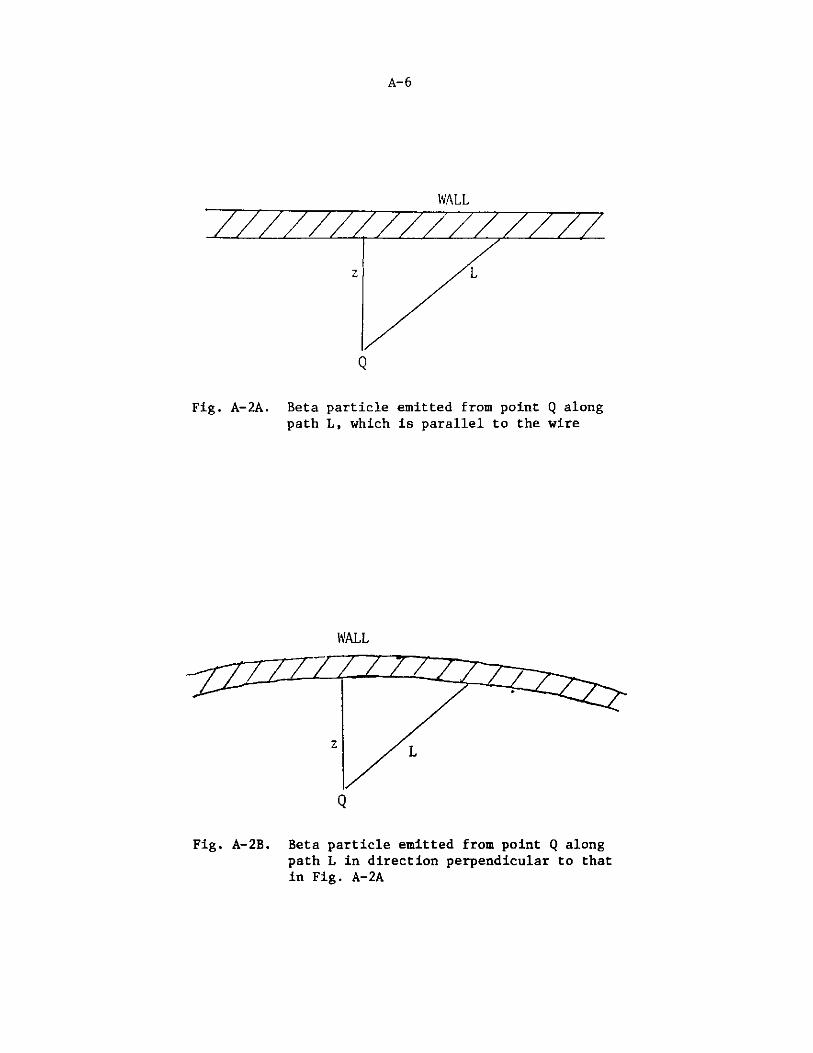
A- 6
WALL
zi L
Q
Fig. A-2A. Beta particle emitted from point Q alongpath L, which is parallel to the wire
WALL
z
Fig. A-2B. Beta particle emitted from point Q alongpath L in direction perpendicular to thatin Fig. A-2A
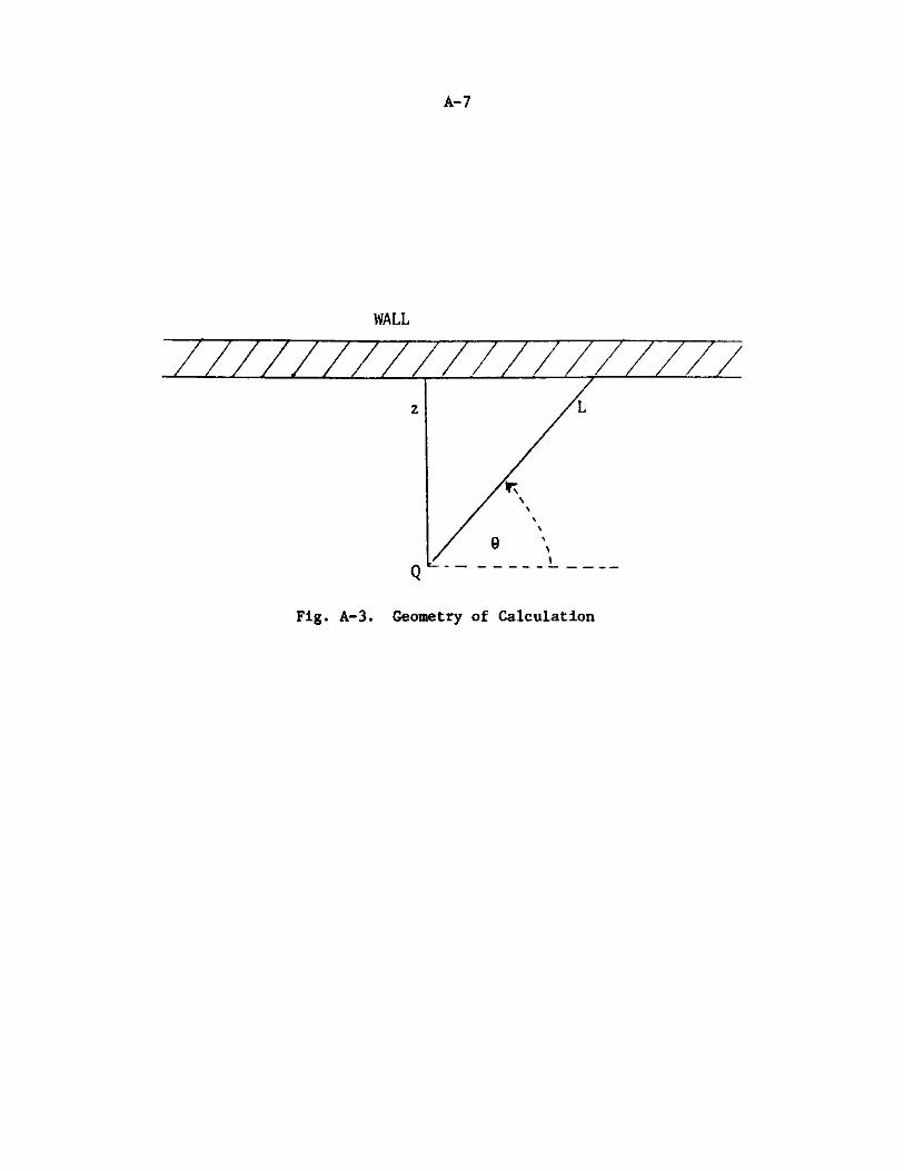
A- 7
WALL
z L
9
Fig. A-3. Geometry of Calculation
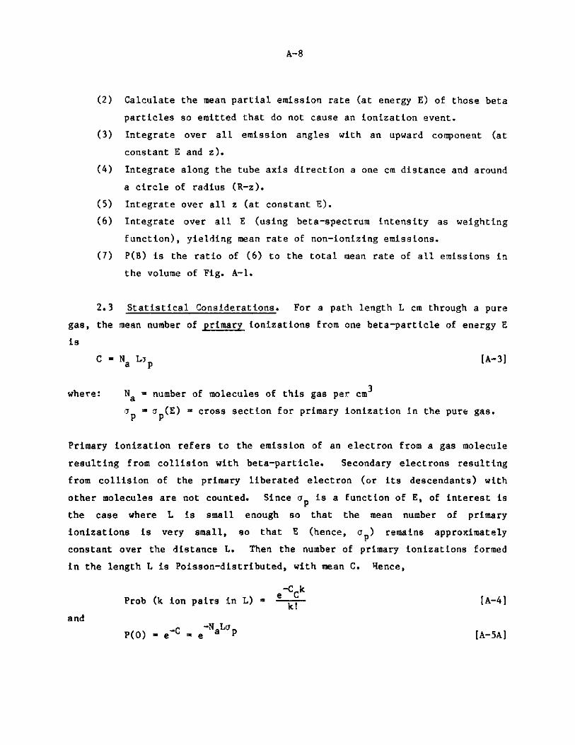
A-8
(2) Calculate the mean partial emission rate (at energy E) of those beta
particles so emitted that do not cause an ionization event.
(3) Integrate over all emission angles with an upward component (at
constant E and z).
(4) Integrate along the tube axis direction a one cm distance and around
a circle of radius (R-z).
(5) Integrate over all z (at constant E).
(6) Integrate over all E (using beta-spectrum intensity as weighting
function), yielding mean rate of non-ionizing emissions.
(7) P(B) is the ratio of (6) to the total mean rate of all emissions in
the volume of Fig. A-1.
2.3 Statistical Considerations. For a path length L cm through a pure
gas, the mean number of primary ionizations from one beta-particle of energy E
is
C - Na L1 p[A-3]
where: Na = number of molecules of this gas per cm3
7p = ap(E) = cross section for primary ionization in the pure gas.
Primary ionization refers to the emission of an electron from a gas molecule
resulting from collision with beta-particle. Secondary electrons resulting
from collision of the primary liberated electron (or its descendants) with
other molecules are not counted. Since ap is a function of E, of interest is
the case where L is small enough so that the mean number of primary
ionizations is very small, so that E (hence, ap) remains approximately
constant over the distance L. Then the number of primary ionizations formed
in the length L is Poisson-distributed, with mean C. Hence,
-C kProb (k ion pairs in L) - ek [A-4]
and-N La
P(O) - e-C = e a p [A-5A]I

A-9
which was earlier written in Eq. [1].*
If several gases are mixed, the results are combined as follows:
With: Na = no. of molecules of Species I per cm3
Na - no. of molecules of Species II per cm3
a' = a'(E) - ionization cross section of Species I
a'=- a"(E) - ionization cross section of Species II
then the probabilities of no primary ionization in molecules of either gas
species are
-N'a'L -N"a"L
P1(0) = e a p and P2 ()e ap [A-5B]
Since these probabilities are independent, the probability of no ionization in
molecules of either species is:
-[(N'a') + N"a")]LP(O) - P1 (0) P2(O) e a p a p -r (A-5C]
with r = N'a' + N"a" [A-5D]a p a p
In the following calculations, certain considerations concerning a class
of radioactive emissions are implicit:
(1) The disintegration rate is Poisson distributed with mean rate S
(2) If a subclass a is considered with probability of occurrence P,
then the number of disintegrations of the a-type is Poisson
distributed with mean rate Spa and the probability of k events (in
unit time) is Poisson with mean Spa.
(3) If a class s is considered with probability P, then k is also
Poisson with mean Spa.
(4) If classes a and a are independent, then if kas - ka + k= - number
of both a and s events, kas is Poisson with mean Spa + Spa- S(pa +
P$).
*P(0) can have a significant value only if C is small (e.g., if C = 7, e~7 -
0.0009). Hence, since the initial beta particle energy is measured in manykilovolts, and since energetic electrons released in primary ionization arerare, the approximation ap = constant is a good one.
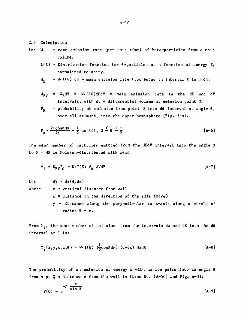
A-10
2.4 Calculation
Let W = mean emission rate (per unit time) of beta-particles from a unit
volume.
I(E) = Distribution function for f-particles as a function of energy E;
normalized to unity.
WE = W. I(E) dE = mean emission rate from betas in interval E to E+dE.
WEV = WEdV = W.I(E)dEdV = mean emission rate in the dE and dV
intervals, with dV = differential volume at emission point Q.
P0 = probability of emission from point Q into d6 interval at angle 0,
over all azimuth, into the upper hemisphere (Fig. A-4).
2TT cos d 1 < (< A-6Po 4nsd cos9d0, 0- 0 2[A-61
The mean number of particles emitted from the dEdV interval into the angle 0
to 0 + d6 is Poisson-distributed with mean
M1 = 1 EVP0 = W".I(E) PO dVdE [A-7]
Let dV dz(dydx)
where z vertical distance from wall
x = distance in the direction of the axis (wire)
y - distance along the perpendicular to x-axis along a circle of
radius R - z.
From M1, the mean number of emissions from the intervals dz and dE into the d
interval at 6 is:
M2 (E,y,x,z,Q) = W I(E) ( cos9d) (dydx) dzdE [A-8]
The probability of an emission of energy E with no ion pairs into an angle 0
from a pt Q a distance z from the wall is (from Eq. [A-5C] and Fig. A-3):
-r zsin 0
P(0) = e [A-9]

A-li
WALL
7d79
Fig. A-4. Emission into d0 interval

A-12
Hence, the mean number of emissions with no primary ionizations is at given
(0,z,E,y,x)
-rM3 (E,y,x, z,0) - WI(E) (CosO) dO e sin 9 (dydx) dzdE [A-10]
Since the event of emitting into one d interval is independent of emitting
into another, summing over all 9 gives the total mean number at constant
(z,E,x,y):
M4(E,x,y,z) =- W.I(E) (dydx) dzdE A(z,E) [A-10a]
with (since r - r(E) )1
A(z,E) f e-(r z/sino )cosO dO [A-10B]0
It may be noted that if rz is very small,
A(z,E) = 1 (for rz = 0) [A-i A]
If rz is very large,
A(z,E) = 0 (for rz >> 1) [A-11B]
A(z,E) is very small except when z is quite close to the wall.
Several of the variables may be analytically integrated. Thus, x is
integrated from 0 to 1 (i.e., for a 1 cm cylindrical section) and y is
integrated around the circle (R - z) in diameter, so
f circledx dy - 2nr(R - z) 27rR [A-iLC]
since* R >> z.
Then, at constant (z,E), the mean number of emissions with no primary
ionizations is:
M5(z,E) -2W-I(E) (2nrR) dz - A(z,E) dE [A-12]
*The entire integrand is very small except for small z (from Eq. [A-iiB].

A-13
Integrating over z (which cannot exceed R, the mean number of emissions with
no primary ionizations (at constant E) is:
RM6(E) a wrRW - I(E) dE f A(z,E) dz
0
To a good approximation (since A(z,E) is very small except for small z),
Rf A(z,E) dz f A(z,E) dz0 0
Then -
M6(E) - R W * I(E) dE f dz f e -(?z/sin a)cos 0 d0 0
I
- =rR W.I(E) dE f cos e [ f erz/sin dz ] d0 0
Let: w- sin dw - sinO dz, dz = sin 9 dw; then, with wi 0at z = 0 and
w - c at z -=o,
1
M6 (E) - R W - I(E) 1 dcossinOd8 )(f e-w dw)dE0 0
The first integral - and the second one - 1.
Then
M6 (E) - it R W " I(E) dE [A-13]
Finally, integrating over E, the mean number of emissions with no primary
ionizations is:
M7 1 ER W max dE [A-14]
Since the total number of emissions (T.E.) of all types from the volume in
Fig. A-1 is W multiplied by the volume, T.E. - W (irR2), and the probability of
emissions with no primary ionization is
M EP(0) - T7. i Jmax (E) dE [A-15]T.E. 2R 0 r(E)

A-14
Na, the number of molecules per cm3 , can also be written as (since the
reference temperature used in this report is 250C):
N = NL 2 3.1 = 3.2393 x 1016 = Cpa L 760 298.15 p =FP
[A-16]
where NL = Loschmidt's number
1 cm 3 of an ideal gas at 00C,
mixture of two gases,
with
= 2.6872 x 10¹⁹ per cm3 = number of molecules in
760 Torr and p is measured in Torr. Then, for a
r = N' a' + N" a" = CFp [f'a' + f"a"]a p a p p p
[A-17A]
N'f = N' + N" =
a a Pand
N"f" aLN' + N" p
a a
where p' and p" are the partial pressures of the respective gases, and p = p'
+ p" is the total pressure. Then Eq. [A-1S] may be stated as
with
P(0) = C >max I(E)
(2CFR) p 0 H(E)[A-18A]
[A-18B]H(E) = f'a'(E) + f"a"(E)p p
For a given gas sample, all the quantities in the question are constants, so
P(O) a:1[A-18C]p
2.5 Computer Computation
Computer computation of Eq. [A-18A] is carried out through the
approximation
Efmax0
I(E )I(F) dE = F AE [A-19]
Fi is a factor for the i-th energy interval; it is discussed below. AE-
values are chosen so that the integrand is almost '.onstant within each AE-
[A-17B]
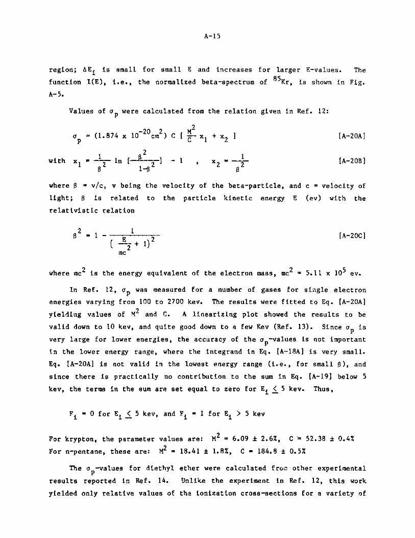
A-15
region; AE1 is small for small E and increases for larger E-values. The
function I(E), i.e., the normalized beta-spectrum of 85Kr, is shown in Fig.
A-5.
Values of ap were calculated from the relation given in Ref. 12:
a = (1.874 x 10⁻²⁰ cm2) C [ C x1 + x2 ] [A-20A]
with x - 2 In [ - 2x 2 2 [A-20B]( 1-S
where 8 S v/c, v being the velocity of the beta-particle, and c = velocity of
light; S is related to the particle kinetic energy E (ev) with the
relativistic relation
2 - 1 2 [A-20C]
2 + 1)
inc
where inc2 is the energy equivalent of the electron mass, mc2 = 5.11 x 10⁵ ev.
In Ref. 12, ap was measured for a number of gases for single electron
energies varying from 100 to 2700 key. The results were fitted to Eq. [A-20A]
yielding values of M2 and C. A linearizing plot showed the results to be
valid down to 10 key, and quite good down to a few Kev (Ref. 13). Since ap is
very large for lower energies, the accuracy of the ap-values is not important
in the lower energy range, where the integrand in Eq. [A-18A] is very small.
Eq. [A-20A] is not valid in the lowest energy range (i.e., for small 8), and
since there is practically no contribution to the sum in Eq. [A-19] below 5
key, the terms in the sum are set equal to zero for Ei < 5 key. Thus,
Fi -0 for Ei <5 key, and Fi -1 for Ei > 5 key
For krypton, the parameter values are: M2 = 6.09 t 2.6%, C- 52.38 * 0.4%
For n-pentane, these are: M2 = 18.41 1.8%, C - 184.8 0.5%
The ap-values for diethyl ether were calculated froin other experimental
results reported in Ref. 14. Unlike the experiment in Ref. 12, this work
yielded only relative values of the ionization cross-sections for a variety of
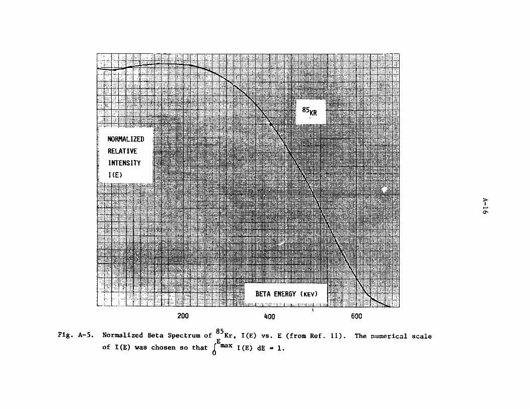
0'-
BETA ENERGY (KEV)
200 400 600
85Normalized Beta Spectrum of Kr, I(E) vs. E (from Ref. 11). The numerical scaleE
of I(E) was chosen so that max I(E) dE = 1.
Fig. A-5.

A-17
gases (using the beta-particles of 85Kr). The relative values were found to
be closely the same over the energy range 75 ev to 500 key. Then
a (diethyl ether)- 0. 930
a pn-pentane)p
For each Ei-value, Eq. [A-20C] gives the ai-value for use in Eq. [A-20B];
hence, the ap(Ei) values for pentane and krypton are derived from Eq.
[A-20A]. The ratio from Ref. 14 then provides ap(Ei) for diethyl ether. From
these ap(E1)-values and the pressures of the gases, H(E1) is evaluated
(Eq. [A-18B]) and the sum calculated as in Eq. [A-19].
Fig. A-6 presents a log-log plot of ap vs E for krypton and for ethyl
ether. The effective ap for each mixture is calculated at each E-value with
Eq. [A-18B].
Fig. A-7 gives a corresponding log-log plot of relative values of the
integrand I(E)/H(E), from Eq. [A-18A] or Eq. [A-19], as a function of E. This
graph illustrates the influence of the various beta-particle energies on the
wall effect calculation. Below the energy at the peak (at ~400 kev), the
integrand increases rapidly with increasing E, because I(E) is almost constant
or slowly changing in this energy range, and a (E) is a rapidly decreasing
function of E. Above the peak, a (E) decreases slowly with increasing E,
while I(E) becomes a rapidly decreasing function of E. It is evident that
most of the contribution to the integral arises from beta particles in the
approximate energy range 150 to 550 key.
P(B) was evaluated for all ten fills with Eq. [A-18A], using the approxi-
mation in Eq. [A-19] for the integral. Results are shown in Section 3.0 (see
Table A). P(B) is the value of PO calculated with neglect of the back-
scattering and shakeoff effects.
3.0 DETERMINATION OF P(C)
Ideally, information on the back scattering effect would be most useful
if its magnitude were available as a function of 0 and E. In the absence of
such information, we use empirical values measured for other purposes which
give backscattering values integrated over 0 and E.
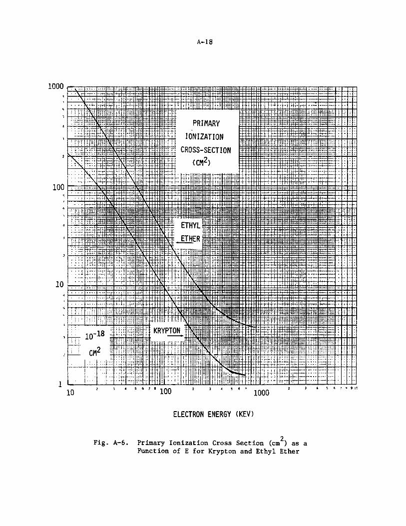
A--18
r .:.. k.: 1 11.Hlt
k-4-4- 4 t4fi
1
- . -- 1-- - - - i -t-'zz7 1'
- -+" f-" --
H--+tH H [I4H llP IIH t[II1HffHHI
PRIMARY
t -. IONIZATION
CROSS-SECTION
(Q 2)
1000
F,
1
2
100
I-I UIN . s4M - -
tILt
i"-1 t
10*
- CM2
2
. - ---4-" ----t--.--1 :_
4-- - f 1
S44
KRYPTON [m
-44ftt1r 4 -L114i : II-
- Ix1-- -I I -- - I-- .r.i ---- E .-'- :.- :1: -:--.- -- =--- I
:jkjpjj . 1.. 1ILW..-fl- i
I .h 4 5 6')'d 100
LFtH1.2 3 4 6 '
FV I~ 4 .. .. .........
1000
liii2 3l 4 S56 'q 9 1
ELECTRON ENERGY (KEV)
Primary Ionization Cross Section (cm2) as aFunction of E for Krypton and Ethyl Ether
rZtN-~4~rF -TYI
E IIT1 HER
10
*
110
Fig. A-6.
4 " 1 !'1 'Hl ! I ll ',11!11:1 1 l l l l 111 ! 1 1 ' l l l 1111
..1 .1 i. .1 .. ...i . .-.... i......1 2 ,
_ -
"
-- - "
" r
," r "
.. " . "
"
T
f"
=H-1-t ki I
Z: Tz
TrF
r
-L LxIilIIIitL
_ .... _.. . . _ t:: -: ..
. . .
';"'i
'uili ~ ~ ~ ~ ~ ~ ~ . . . .... 4. tiril t l :' "Tt'+I 1",1"" . 1.-.1
i -. i .y iJ 1 { I J i:J J f - -+ i -. J.- L. _-+ p4 w" "..
R i. N."
1 [ 1 1 ' 1 1
EtI I I
f.I
I
rs
1 1 1 1
" ... ,_'-. + J w r
. . "r" .i Leh }+". -"
I
1}rI r. If t#
1 t 1 1" 11 1 .
t1.
'I
=r-171.
-
rri
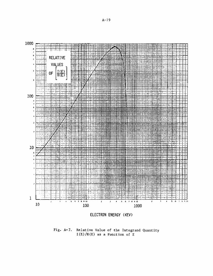
A- 19
- . -
ELATIVE
VALUES
F [1(E)[1(E) I1
F411
_i _
I'lN f F- - Y
1000d
6
3
2
100
6
c
3
2
10a
1
mtrl
: 1:_r .1IF] I Kbk'i~ t t1 fri tfrft 4 tft+
" 1 I I 1 r I 1 1 r " I r
F
I
. .. . . 1 1 i ~ I f 1 f r _ _ I 1 1 t'-4- 'r r ." " }} 1t"" . wry ""."
. . . " .. . ... 1 "1 i 4 1" ' ' 1 I t 1 T t, " I I "1 '-rtt f tr+.} /-"1 "-F t.- .- +" ..
41 . . .. . ". " f } " r 1 f _ I .. }_I " r - 1 L 1 '+ i "t ".If t""-t' 1 I ?" Y+' r Tr f . "*".
I I I i I I r I 1
2 3 4 5 6 7 8 910
10002 3 4 5 6 7 R 0
ELECTRON ENERGY (KEV)
Fig. A-7. Relative Value of the Integrand QuantityI(E)/H(E) as a Function of E
-R
-~E~E
- - -
10. 1 4t 5 6 7 8A9 10
100
. ter. . " " " :w.14 91-1 1
-' I r ,-'i' r "t
-n~ -3-i-t
t: f . .
-
- * -
.. ..-.... , rL
-. "_ - . - .er - .
-t 1t
f f-
y
y
-t -H r-.-. ... '.r, .....
. . . .... ..
FI2HIttl f1
-. rt t -ft- i
r t . . .- _..

A-20
These measurements were made in experiments Aesigned to determine the
counting efficiency of a GM tube or proportional counter for measuring the
emission rates from thin solid beta-emitting radioactive samples mounted on
metal plates. In one configuration (a), a sample plate with deposited
radioactivity was placed immediately outside and parallel to the very thin
window of an "end-window" GM tube. The radioactivity was very close to the
active discharge region, the average solid angle (relative to 4 ) subtended at
the sample being ~25%. It was found that the counting efficiency exceeded the
value calculable from the solid angle because some of the beta-particles
emitted into the plate were backscattered through the window and were
counted. Calibration of the backscattering magnitude was made by comparing
the measured counting rate of activity mounted on a metal plate with that of
the same amount of activity mounted on a very thin plastic film, too thin to
cause backscattering. Another variation to this approach involved placing
metal plates immediately below the activity deposited on a thin plastic film.
In another configuration (s), the sample plates were placed inside a flow
proportional counter, in which the samples rested on or near one wall, and the
relative solid angle subtended was ~50%. The saturation counting rates were
measured for backings of various atomic numbers Z and for several maximum beta
energies and compared to the known disintegration rates.
The general results of these measurements were:
(1) For a given atomic number (Z) substrate, the fraction of beta-
particles emitted into the substrate that are backscattered (Frb)
increases (with increasing substrate thickness) to a saturation
value that depends mildly on the beta-particle maximum energy and
more sharply upon Z. [For our application, the MEP wall thickness
(of copper) is larger than the saturation value.]
(2) Saturation Frb increases with the atomic number of the substrate.
(3) The value of Frb at the saturation substrate thickness (at a given
Z) is about the same at various values of the maximum beta-energy.
(4) The back-scattered beta-particles are degraded in energy.
(5) For a source outside of the counter, the angular distribution of the
backscattered beta-particles is anisotropic, tending to favor the
direction perpendicular to the substrate. This implies that the
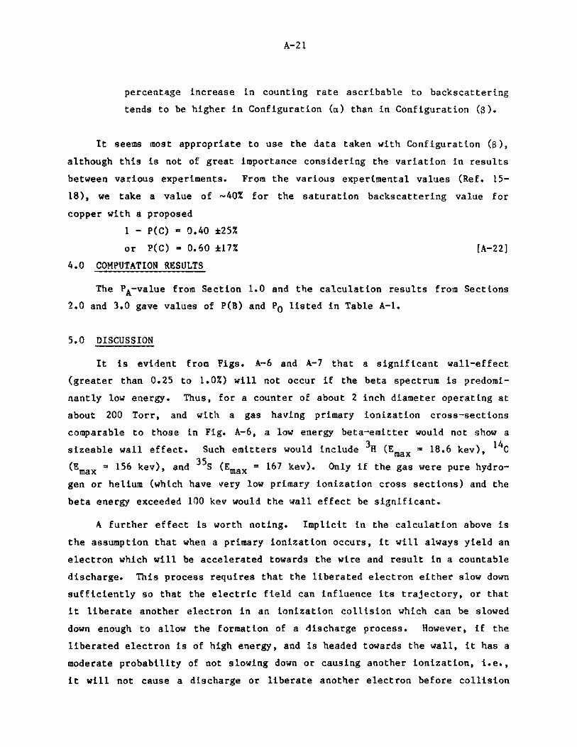
A-21
percentage increase in counting rate ascribable to backscattering
tends to be higher in Configuration (a) than in Configuration (s).
It seems most appropriate to use the data taken with Configuration (),although this is not of great importance considering the variation in results
between various experiments. From the various experimental values (Ref. 15-
18), we take a value of ~40% for the saturation backscattering value for
copper with a proposed
1 - P(C) = 0.40 *25%
or P(C) = 0.60 17% [A-22]
4.0 COMPUTATION RESULTS
The PA-value from Section 1.0 and the calculation results from Sections
2.0 and 3.0 gave values of P(B) and PO listed in Table A-1.
5.0 DISCUSSION
It is evident from Figs. A-6 and A-7 that a significant wall-effect
(greater than 0.25 to 1.0%) will not occur if the beta spectrum is predomi-
nantly low energy. Thus, for a counter of about 2 inch diameter operating at
about 200 Torr, and with a gas having primary ionization cross-sections
comparable to those in Fig. A-6, a low energy beta-emitter would not show a
sizeable wall effect. Such emitters would include 3H (Emax = 18.6 kev), 14C
(Emax = 156 kev), and 35S (Emax = 167 kev). Only if the gas were pure hydro-
gen or helium (which have very low primary ionization cross sections) and the
beta energy exceeded 100 key would the wall effect be significant.
A further effect is worth noting. Implicit in the calculation above is
the assumption that when a primary ionization occurs, it will always yield an
electron which will be accelerated towards the wire and result in a countable
discharge. This process requires that the liberated electron either slow down
sufficiently so that the electric field can influence its trajectory, or that
it liberate another electron in an ionization collision which can be slowed
down enough to allow the formation of a discharge process. However, if the
liberated electron is of high energy, and is headed towards the wall, it has a
moderate probability of not slowing down or causing another ionization, i.e.,
it will not cause a discharge or liberate another electron before collision

A-22
with the wall. If this effect is significant, then the above calculation
underestimates the wall-effect.
Except for the lowest energy liberated electrons, there is indeed a high
correlation between the directions of the beta-particle and liberated electron
trajectories. However, losing a discharge from an ionization electron can
occur with significant probability only if the liberated electron energy ELe
is itself high enough. This situation can occur only with very low proba-
bility, because the liberated electron energy distribution only goes out to a
maximum electron energy of one-half the beta-particle energy and the distribu-
tion has an intensity variation proportional to 1/EL2 with a cutoff at very
low energy.1 9 Thus, most of the electrons liberated in primary ionization,
even from the highest energy beta-particles, have low energy, and, as is
evident from Fig. A-6, these will almost certainly ionize the gas.
Table A-1
COMPUTED WALL-EFFECT RESULTS
Total GasPressure Percent
Fill No. (Torr) Ethyl Ether P(B) P0 (a)
1 201.84 7.51% 0.00965 0.0045
2 201.84 7.50 0.00965 0.0045
3 205.48 7.50 0.00948 0.0044
4 277.40 7.51 0.00702 0.0033
5 204.51 10.00 0.00908 0.0042
6 335.41 10.00 0.00553 0.0026
7 325.93 10.00 0.00569 0.0027
8 324.99 10.00 0.00571 0.0027
9 199.90 10.00 0.00928 0.0044
10 224.70 10.01 0.00826 0.0039
(a) PO given in Eq. [A-1C], with PA = 0.78, P(C) 0.6, from Eq. [A-22].
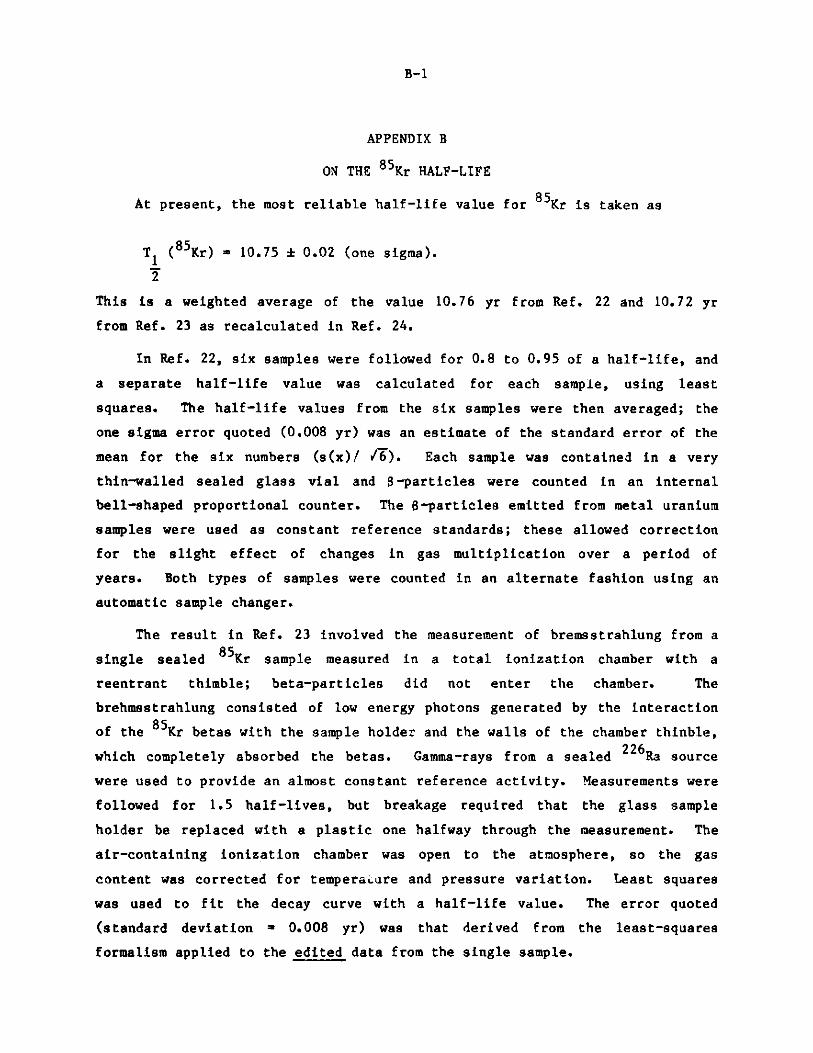
B-1
APPENDIX B
ON THE 8 5Kr HALF-LIFE
At present, the most reliable half-life value for 85Kr is taken as
T (85Kr) - 10.75 * 0.02 (one sigma).
2
This is a weighted average of the value 10.76 yr from Ref. 22 and 10.72 yr
from Ref. 23 as recalculated in Ref. 24.
In Ref. 22, six samples were followed for 0.8 to 0.95 of a half-life, and
a separate half-life value was calculated for each sample, using least
squares. The half-life values from the six samples were then averaged; the
one sigma error quoted (0.008 yr) was an estimate of the standard error of the
mean for the six numbers (s(x)/ /6). Each sample was contained in a very
thin-walled sealed glass vial and S-particles were counted in an internal
bell-shaped proportional counter. The 8-particles emitted from metal uranium
samples were used as constant reference standards; these allowed correction
for the slight effect of changes in gas multiplication over a period of
years. Both types of samples were counted in an alternate fashion using an
automatic sample changer.
The result in Ref. 23 involved the measurement of bremsstrahlung from a
single sealed 85Kr sample measured in a total ionization chamber with a
reentrant thimble; beta-particles did not enter the chamber. The
brehmsstrahlung consisted of low energy photons generated by the interaction
of the 8 5Kr betas with the sample holder and the walls of the chamber thimble,
which completely absorbed the betas. Gamma-rays from a sealed 2 26Ra source
were used to provide an almost constant reference activity. Measurements were
followed for 1.5 half-lives, but breakage required that the glass sample
holder be replaced with a plastic one halfway through the measurement. The
air-containing ionization chamber was open to the atmosphere, so the gas
content was corrected for temperature and pressure variation. Least squares
was used to fit the decay curve with a half-life value. The error quoted
(standard deviation - 0.008 yr) was that derived from the least-squares
formalism applied to the edited data from the single sample.

B-2
The results of both experiments have been combined here to give the value
10.75 yr, greater weight being given to Ref. 22, because of the redundancy of
samples and the greater reliability of counting -particles in an internal
counter as compared to measuring ionization from the relatively low energy
bremsstrahlung photons with an external chamber. The errors calculated from
each experiment (0.008 yr) were much smaller than the difference in half-life
values (~ 0.04 yr); the estimated error has therefore been arbitrarily enlarged
to 0.02 yr. Other measured half-life values of 8 5 Kr have not been included in
the averaging, because the results had much larger errors.
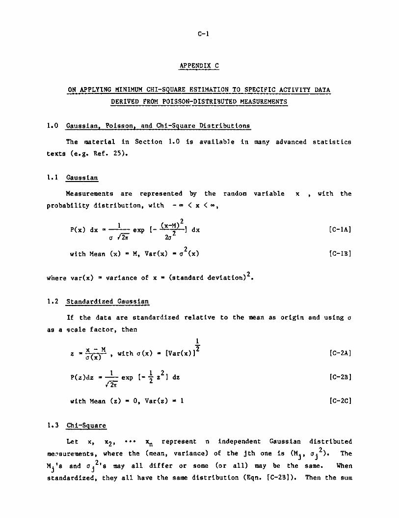
C-1
APPENDIX C
ON APPLYING MINIMUM CHI-SQUARE ESTIMATION TO SPECIFIC ACTIVITY DATA
DERIVED FROM POISSON-DISTRIBUTED MEASUREMENTS
1.0 Gaussian, Poisson, and Chi-Square Distributions
The material in Section 1.0 is available in many advanced statistics
texts (e.g. Ref. 25).
1.1 Gaussian
Measurements are represented by the random variable x , with the
probability distribution, with - c < x < c,
P(x) dx = exp [- - -] dx [C-1A]
a /2n 2a
with Mean (x) = M, Var(x) - a2 x) [C-1B]
where var(x) - variance of x = (standard deviation)2 .
1.2 Standardized Gaussian
If the data are standardized relative to the mean as origin and using a
as a scale factor, then
1
z = x - M , with a(x) _ [Var(x)] 2 [C-2A]a Cx)
P(z)dz -1exp [- 2z ] dz [C-2B]
with Mean (z) - 0, Var(z) - 1 [C-2C]
1.3 Chi-Square
Let x, x2, *.. xn represent n independent Gaussian distributed
measurements, where the (mean, variance) of the jth one is (M, a2). The
M 's and a 2's may all differ or some (or all) may be the same. When
standardized, they all have the same distribution (Eqn. [C-2B]). Then the sum
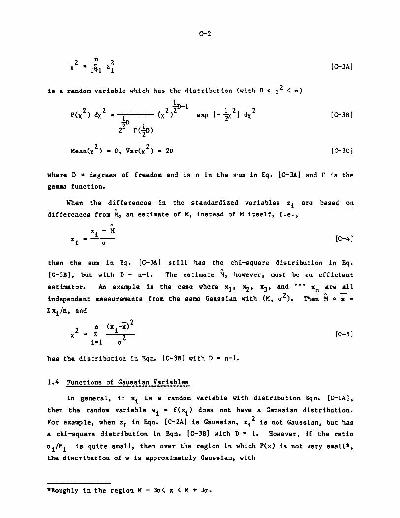
C-2
X2 E z [C-3A]
is a random variable which has the distribution (with 0 <X2<)
2 2 ___-2 1 2 2P(X ) dX - 1 (X ) exp [--X ] dX [C-3B]
-D22 r(D)
222
Mean(X2) - D, Var(X2) = 2D [C-3C]
where D - degrees of freedom and is n in the sum in Eq. [C-3A] and r is the
gamma function.
When the differences in the standardized variables zi are based on
differences from M, an estimate of M, instead of M itself, i.e.,
x - M
zt [C-4J
then the sum in Eq. [C-3A] still has the chi-square distribution in Eq.
[C-3B], but with D - n-1. The estimate M, however, must be an efficient
estimator. An example is the case where x1, x2, x 3 , and **Xn are all
independent measurements from the same Gaussian with (M, a2). Then M - x -
E xi/n, and
2 n (xi-x)2x - E 2 [C-5]
i-1 a
has the distribution in Eqn. [C-3B] with D a n-1.
1.4 Functions of Gaussian Variables
In general, if xi is a random variable with distribution Eqn. [C-1A],
then the random variable wi - f(xi) does not have a Gaussian distribution.
For example, when zi in Eqn. [C-2A] is Gaussian, zit is not Gaussian, but has
a chi-square distribution in Eqn. [C-3B] with D - 1. However, if the ratio
ai/Mi is quite small, then over the region in which P(x) is not very small*,
the distribution of w is approximately Gaussian, with
*Roughly in the region M - 3a< x < M + 3a.

C-3
Mean(w) w f(M) and Var(w) = [( d) 2 Var(x) [C-6]
where the derivative is evaluated at x - M.
1.5 Poisson
In radioactive decay processes, if k - the number of disintegrations in a
fixed time interval T, then k has a Poisson distribution
-M -kP(k) - e kMean (k) - M, [C-7]
where k is an integer and Var(k) - M. If M is large enough, say >100, the
Poisson distribution may be approximated by the Gaussian in Eqn. [C-1AJ, with
Mean(k) - Var(k) - M and standard deviation - / and k is treated
approximately as a continuous random variable. If U - g(k), then, if
/M/M - 1//H is small, then U may be treated as approximately Gaussian with
Mean (U) = g(M) and [C-8A]
Var(U) k()2 Var(k). (1) 2 M [C-8B]
1.6 Chi-Square with Poisson-based Data
If the M-values are large enough, then standardized variables based on
Poisson-distributed quantities may be combined into the chi-square form.
There is one modification, however, resulting from the fact that for Poisson
data, Var(x) = Mean(x) - M. Thus, if the xi's in Eqn. [C-5] are Poisson
variables, then X 2 may be written in the form
2 n (xi-) 2 [X *ii _[C-91
x
since (for the Poisson), a2 - M, hence x is shown as an estimate of Var(x) as
well as of M. X2 in Eqn. [C-9] can be shown to have the approximate chi-
square distribution with (n-1) degrees of freedom.

C-4
2.0 MINIMUM CHI-SQUARE FOR ESTIMATION
Consider n random variables xi where each xi is a random variable which
is a function of a Poisson random variable ki. Then, approximately, the xi's
are Gaussian and the sum of the squared standardized quantities is chi-square
distributed. Suppose each xi is a function of the same unknown quantity, V,
and we wish to estimate the V-value from some combination of the n values of
xi. There are various efficient schemes for such estimation, among which are
maximum likelihood and minimum chi-square. Under the latter, the best
estimate is that value of V which minimizes the sum representing chi-square.
3.0 APPLICATION OF MINIMUM CHI-SQUARE TO EVALUATION OF SPECIFIC ACTIVITY FROM
MEP MEASUREMENTS
To formulate the appropriate form of chi-square = Q, the following
definitions apply to one gas fill at a given high voltage value
S disintegration rate of that portion of the gas fill contained in the
squat cylindrical box one cm along the tube axis and with MEP radius
(see Fig. A-1).
n = number of different measurements made with different tube lengths.
Li = length of tube as indicated by position of precision scale. This was
calibrated at the initial disassembly of the counter.
Si = estimate of S, calculated from measurement at i-th position.
Al = plus (or minus) deviation of each Li from the actual piston-to-piston
length due to nonreproducibility arising from gasket thickness
variation in reassembly. A1 is unknown for the various reassemblies,
but is small because the gold gasket itself was <1 mm diameter.
Although its value is not known, A1 is the same for all sequential
fills in which reassembly did not occur.
A2 = end effect decrement in length for a particular fill. It is a function
of high voltage, but not of tube length.
A = A2 t A 1 , depending on sign of A1l
EL1 - Li - A - effective length of tube at the ith piston position.
N1 = total counts measured at ith position.
T = livetime of ith counting period.
c = N1/Ti - measured counting rate at ith position
t= elapsed time of ith count since reference date.

c-5
Di - exti - decay correction to reference date
Ci - Dici - decay corrected counting rate.
C D c D NS. E - i) aiNi , [C-10]i ELi ELi ELTi
D
with a - Di Then,i i
2 2 2a (S ) a (S ) a (N ) mean (N )
2 2 * 2 [C-iA][mean (Si)] Si [mean (Ni)] [mean (Ni) ] i
or 2
2(Si) - I[C-11B)
Then the statistical weight for Si is
Nw -- 1 i [C-11C]
2(Si) S2
The weighted average as an estimate of S is
- 1 n n
S=- J w1Si, where W E w [C-121
Then Q, which is chi-square distributed with DF = n-1, is
n [S - estimate(mean(S )]2
estimate [a (S )]
Hence,
n (Si-S)2 n -2Q=- E1 2 a i 1w (Si-S) [C-13]
s= 2/Ni
It is evident that, since the value of each Si depends upon the A-value,
then Q is a function of A. The best estimate A is the A-value which minimizes
Q. This may be found by choosing a starting value for A, computing Q and then
using a converging step procedure to iterate to a minimum value. Given the A-
estimate, as the A-value used in the final Q calculation, the corresponding

C-6
S-value is the estimate of S. As noted in the body of the report, this value
is the same as that derived by using weighted least squares to calculate the
slope of the line representing the counting rate as a function of Li.

a
Distribution for ANL-87-34
Internal:
W. C. Bentley (5) S. J. Rymas (2)F. A. Cafasso E. P. SteinbergM. S. Freedman H. P. Yule (5)J. Gray (5) ANL Patent DepartmentJ. P. Hughes ANL Contract FileM. Inokuti ANL LibrariesA. H. Jaffey (55) TIS Files (5)
External:
DOE-TIC, for distribution per UC-4 (105)Manager, Chicago Operations Office, DOEChemistry Division Review Committee:
A. C. Albrecht, Cornell U.E. R. Davidson, Indiana U.E. C. Hoffman, Lawrence Berkeley Lab.T. J. Meyer, U. North CarolinaE. S. Pierce, Kensington, MDA. M. El-Sayed, U. California, Los AngelesW. W. Schulz, Rockwell Hanford
A. Boni, Savannah River Lab.G. A. Cowan, Los Alamos National Lab.T. V. Crawford, Savannah River Lab.L. Currie, National Bu. Standards, GaithersburgR. Davis, U. PennsylvaniaC. Gatrousis, Lawrence Livermore National Lab.S. Katcoff, Brookhaven National Lab.J. B. Knox, Lawrence Livermore National Lab.L. Machta, NOAA, Silver SpringW. B. Mann, National Bu. Standards, GaithersburgA. Mason, Los Alamos National Lab.W. L. Nicholson, Pacific Northwest Lab.A. Spernol, EURATOM, Geel, BelgiumF. H. Tingey, U. IdahoA. Turkevich, U. Chicago