theoretical computer science course presentation
TRANSCRIPT
1
Theoretical Computer Science
Course Presentation

2
Objectives and motivations
Why Theoretical Computer Science in an Engineering Curriculum?
Theory is stimulated by practice,
practice is helped by theory:
generality, rigor, “control”
• Engineer is a person who:
– Applies theory to practice
– Extracts theory from practice
3
• Deeply and critically understand the principles of
Computer Science (careful re-view of basic CS
notions)
• Build solid ground to understand and master
innovation (e.g.: multimedia, modeling of concurrent
and wireless computation)
• Theory as an antidote to overspecialization and as a
support to interdisciplinary studies
4
• Throw a bridge between basic, applicative courses and
more advanced ones (SW engineering, Hardware and
computer architecture, distributed systems…)
• Direct application of some notions of TCS to practical
cases: in follow-up courses such as Formal Languages
and Compilers, Formal Methods, and thesis work

5
The program (1/2)
• Modeling in Computer Science
(How to describe a problem and its solution):
Do not go deep into specific models, rather
provide ability to understand models and invent new
ones
• Theory of Computation:
what can I do by means of a computer
(which problems can I solve)?
6
The program (2/2)
• Complexity theory:
how much does it cost to solve a problem through a
computer?
• Only the basics: further developments in follow-up
courses
7
Organization (1/3)
• Requirements :
– Basics of Computer science (CS 1)
– Elements of discrete mathematics ([Algebra and Logic])
• Lesson and practice classes (all rather classical
style…)
– Student-teacher interaction is quite appreciated:
• In classroom
• In my office
• By Email (administrative matters and to fix face-to-face meetings)
8
Organization (2/3)
• Exam tests ability to apply, not to repeat:
mainly written
can consult textbooks and notes
not repetitive, challenging (hopefully)
• Standard written (+ possibly oral) exams on the whole
program
– No midterm exams, forbidden by faculty rules
– Details will be notified in due time…
9
Organization (3/3)
• Teaching material:
– Official text :
• Ghezzi/Mandrioli: Theoretical Foundations of Computer Science [Wiley]
– Not re-printed by the publisher: you can photocopy it, possibly in a legal way
(ask the teacher how)
• In Italian: Carlo Ghezzi, Dino Mandrioli, Informatica Teorica, UTET.
– Dino Mandrioli, Paola Spoletini, MATHEMATICAL LOGIC FOR
COMPUTER SCIENCE: an Introduction, Esculapio Società Editrice, 2010.
– English translation of the Italian Practice book: Mandrioli, Lavazza, Morzenti,
San Pietro, Spoletini, Esercizi di informatica teorica, 3rd edition, Esculapio)
– Previous exam texts with solutions, some in Italian (sorry…) MOST in English
– Lesson slides (NOT to use as a substitute of the text book!), exercise book, notices
and various material on the course available for download at the web page:
http://home.dei.polimi.it/morzenti/tcs.html

10
Models in Computer Science
• Not only discrete vs. continuous(bits & bytes vs. real numbers and continuous functions)
• Operational models(abstract machines, dynamic systems, …)based on the concept of a state and of means (operations) torepresent its evolution (w.r.t. “time”)
• Descriptive modelsaimed at expressing properties (desired of feared) of the modeled system, rather than its functioning as an evolutionthrough states
11
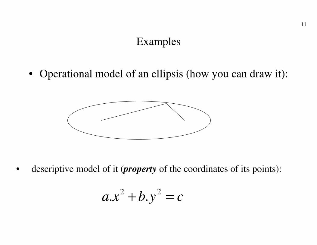
Examples
• Operational model of an ellipsis (how you can draw it):
• descriptive model of it (property of the coordinates of its points):
cybxa =+ 22 ..
12
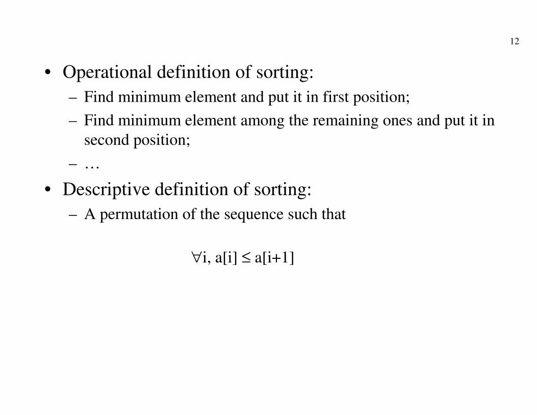
• Operational definition of sorting:
– Find minimum element and put it in first position;
– Find minimum element among the remaining ones and put it in
second position;
– …
• Descriptive definition of sorting:
– A permutation of the sequence such that
∀i, a[i] ≤ a[i+1]
13
• In fact, differences between operational and descriptive
models are not so sharp
• It is however a very useful classification of models
– Corresponds closely to different “attitudes” that people adopt
when reasoning on systems

14
A first, fundamental, “meta”model:
the language
• Italian, French, English, …
• C, Pascal, Ada, …
but also:
• Graphics
• Music
• Multimedia, ...

15
Elements of a language
• Alphabet or vocabulary
(from a mathematical viewpoint these are synonyms):
Finite set of basic symbols
{a,b,c, …z}
{0,1}
{Do, Re, Mi, …}
ASCII char set
...
16
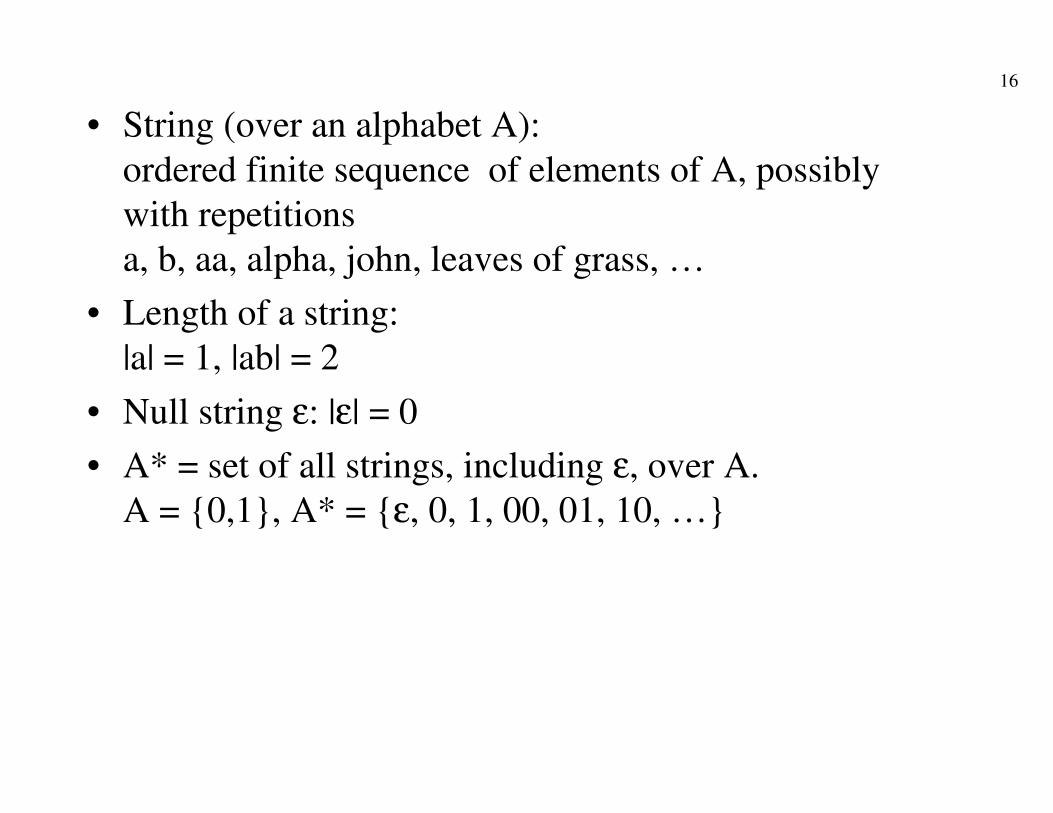
• String (over an alphabet A):
ordered finite sequence of elements of A, possibly
with repetitions
a, b, aa, alpha, john, leaves of grass, …
• Length of a string:
|a| = 1, |ab| = 2
• Null string ε: |ε| = 0
• A* = set of all strings, including ε, over A.
A = {0,1}, A* = {ε, 0, 1, 00, 01, 10, …}
17
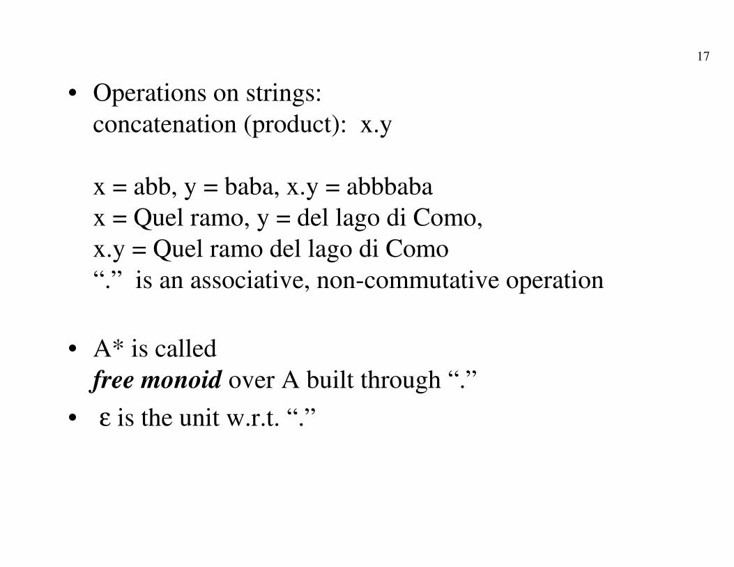
• Operations on strings:
concatenation (product): x.y
x = abb, y = baba, x.y = abbbaba
x = Quel ramo, y = del lago di Como,
x.y = Quel ramo del lago di Como
“.” is an associative, non-commutative operation
• A* is called
free monoid over A built through “.”
• ε is the unit w.r.t. “.”
18
Language
• L subset of A*: (L⊆ A*)
Italian, C, Pascal, … but also:
sequences of 0 and 1 with an even number of 1
the set of musical scores in F minor
symmetric square matrices
…
• It is a very broad notion, somehow universal

19
Operations on languages
• Set theoretic operations:
∪, ∩, L1 -L2, ¬L = A* - L, )( LL ¬=
• Concatenation (of languages):
L1 .L2 = {x.y| x ∈ L1, y ∈ L2}
L1 = {0,1}*, L2 = {a,b}* ;
L1 .L2 = {ε, 0,1, 0a, 11b, abb, 10ba, ….} NB: ab1 not included!
20
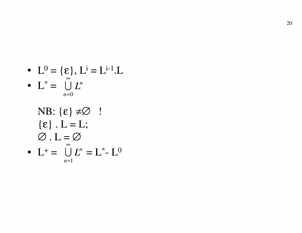
• L0 = {ε}, Li = Li-1.L
• L* =
NB: {ε} ≠∅ !
{ε} . L = L;
∅ . L = ∅
• L+ = = L*- L0
n
n
L∞
=0
U
n
n
L∞
=1
U
21
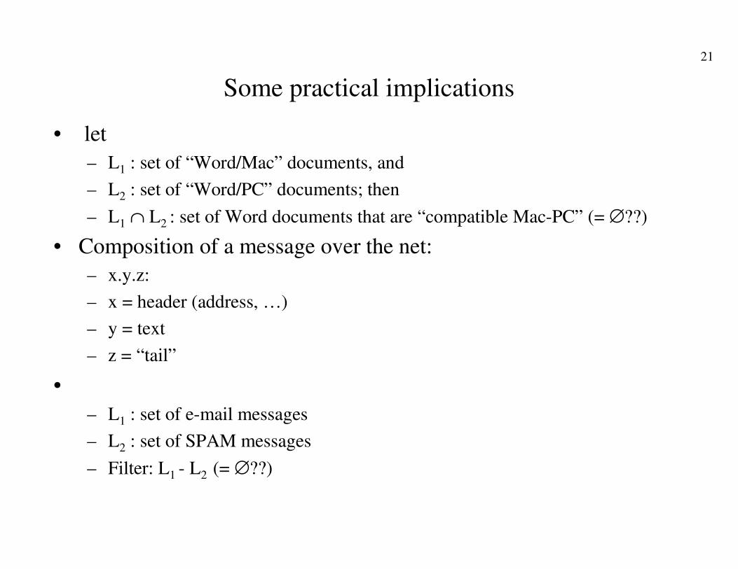
Some practical implications
• let
– L1 : set of “Word/Mac” documents, and
– L2 : set of “Word/PC” documents; then
– L1 ∩ L2 : set of Word documents that are “compatible Mac-PC” (= ∅??)
• Composition of a message over the net:
– x.y.z:
– x = header (address, …)
– y = text
– z = “tail”
•
– L1 : set of e-mail messages
– L2 : set of SPAM messages
– Filter: L1 - L2 (= ∅??)
22
• A language is a means of expression …
• Of a problem
• x ∈ L?
– Is a message correct?
– Is a program correct?
– y = x2 ?
– z = Det(A)? (is z the determinant of matrix A)
– Is the soundtrack of a movie well synchronized with the
video?

23
• y = τ(x)
τ : translation is a function from L1 to L2
– τ 1 : double the “1” (1 --> 11):
τ 1(0010110) = 0011011110, …
– τ 2 : change a with b and viceversa (a <---> b):
τ 2(abbbaa) = baaabb, …
– Other examples:
• File compression
• Self-correcting protocols
• Computer language compilation
• translation Italian ---> English
Translation
24
Conclusion
• The notion of language and the basic associated operations
provide a very general and expressive means to describe any
type of systems, their properties and related problems:
– Compute the determinant of a matrix;
– Determine if a bridge will collapse under a certain load;
– ….
• Notice that, after all, in a computer any information is a string of
bits (hence a string of some language…)
25
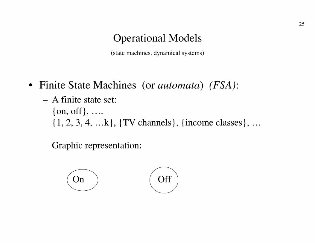
Operational Models
(state machines, dynamical systems)
• Finite State Machines (or automata) (FSA):
– A finite state set:
{on, off}, ….
{1, 2, 3, 4, …k}, {TV channels}, {income classes}, …
Graphic representation:
On Off

26
Commands (input) and state transitions
• Two very simple flip-flops:
On OffT
T
On Off
R
S
SR
Turning a light on and off, ...
27
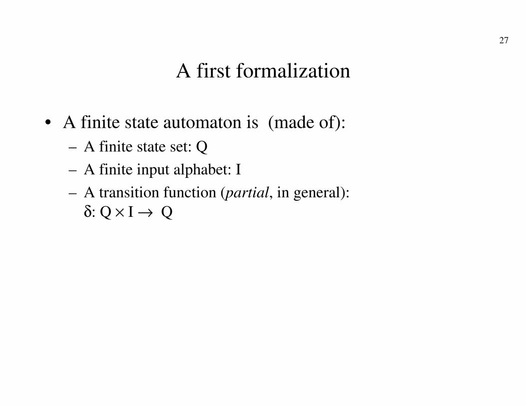
A first formalization
• A finite state automaton is (made of):
– A finite state set: Q
– A finite input alphabet: I
– A transition function (partial, in general):
δ: Q × I → Q

28
Automata as language recognizers (or acceptors)
(x ∈ L?)
• A move sequence starts from an initial state and it is
accepting if it reaches a final (or accepting) state.
q0 q1
10 0
1
L = {strings with an even number of “1” any number of “0”}

29
Formalization of the notion of acceptance of language L
• Move sequence:
– δ∗: Q × I∗ → Q
δ∗ defined inductively from δ, by induction on the string length
δ∗ (q,ε) = q
δ∗ (q,y.i) = δ(δ∗ (q,y), i)
• Initial state: q0 ∈ Q
• Set of final, or accepting states: F ⊆ Q
• Acceptance: x ∈ L ↔ δ∗ (q0,x) ∈ F
30
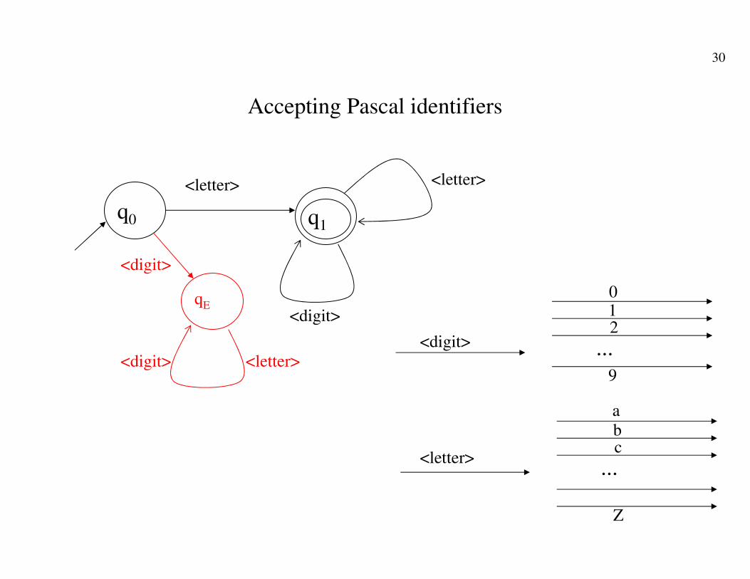
Accepting Pascal identifiers
q0 q1
<letter> <letter>
<digit>
<letter>
abc
Z
...
qE
<digit>
<digit> <letter><digit>
012
9
...
31
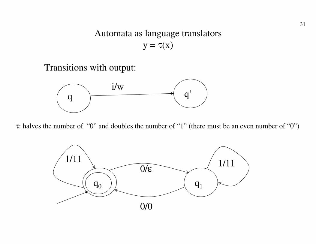
Automata as language translators
y = τ(x)
Transitions with output:
q q’i/w
τ: halves the number of “0” and doubles the number of “1” (there must be an even number of “0”)
q0 q1
0/ε1/11 1/11
0/0
32
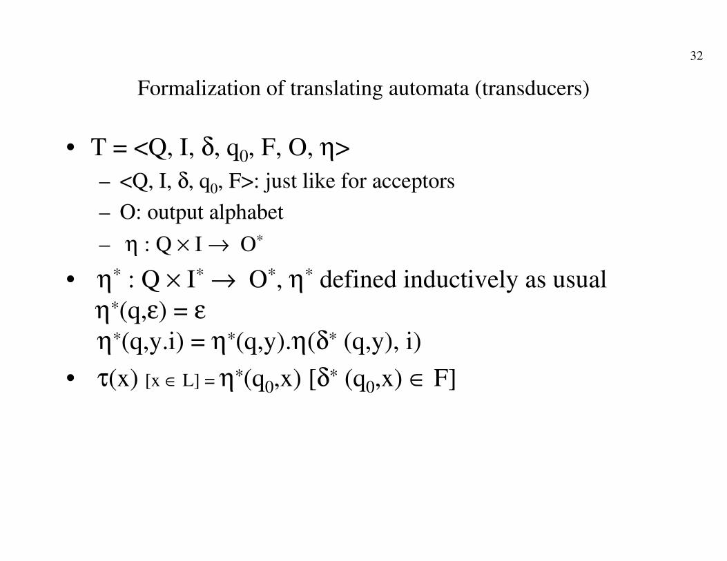
Formalization of translating automata (transducers)
• T = <Q, I, δ, q0, F, O, η>
– <Q, I, δ, q0, F>: just like for acceptors
– O: output alphabet
– η : Q × I → O*
• η* : Q × I* → O*, η* defined inductively as usual
η∗(q,ε) = εη∗(q,y.i) = η∗(q,y).η(δ∗ (q,y), i)
• τ(x) [x ∈ L] = η∗(q0,x) [δ∗ (q0,x) ∈ F]
33
Analysis of the finite state model
(for the synthesis refer to other courses - e.g. on digital circuits)
• Very simple, intuitive model, applied in various sectors, also
outside computer science
• Is there a price for this simplicity?
• …
• A first, fundamental property: the cyclic behavior of finite
automata

34
a
a
b
a
a
b
b
b
b
b
a
q1 q2
q3
q0
q4q5
q6 q7
q9
q8
There is a cycle q1 ----aabab---> q1
If one goes through the cycle once, then one can also go through
it 2, 3, …, n, … 0 times =========>

35
Formally:
• If x ∈ L and |x| > |Q| there exists a q ∈ Q and a w ∈ I+ such that:
• x = ywz
• δ∗ (q,w) = q
Then ywnz ∈ L, ∀ n ≥ 0 :
• This is known as the Pumping Lemma
36
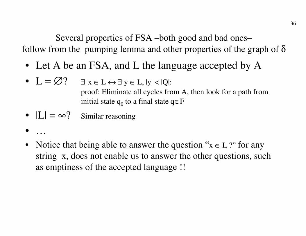
Several properties of FSA –both good and bad ones–
follow from the pumping lemma and other properties of the graph of δ
• Let A be an FSA, and L the language accepted by A
• L = ∅? ∃ x ∈ L ↔ ∃ y ∈ L, |y| < |Q|:
proof: Eliminate all cycles from A, then look for a path from
initial state q0 to a final state q∈F
• |L| = ∞? Similar reasoning
• …
• Notice that being able to answer the question “x ∈ L ?” for any
string x, does not enable us to answer the other questions, such
as emptiness of the accepted language !!

37
A “negative” consequence of the Pumping Lemma (PL)
• Is the language L = {anbn|n > 0} recognized by any FSA?
– Put it another way: can we count using a FSA?
• Let us assume so (by contradiction):
• Consider x = ambm, with m > |Q| and apply the PL: then x = ywz and xwny∈L ∀n
• There are 3 possible cases:
– x = ywz, w = ak , k > 0 ====> am+r.kbm ∈ L, ∀r : this cannot be (it contradicts the assumption)
– x = ywz, w = bk , k > 0 ====> idem
– x = ywz, w = ak bs , k,s > 0 ====> am-kakbs akbsbm-s ∈ L: this cannot be (it contradicts the assumption)
38
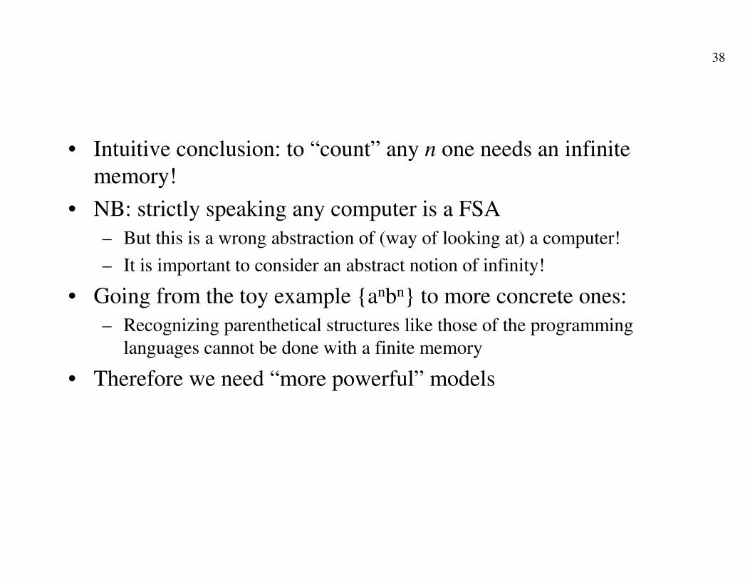
• Intuitive conclusion: to “count” any n one needs an infinite
memory!
• NB: strictly speaking any computer is a FSA
– But this is a wrong abstraction of (way of looking at) a computer!
– It is important to consider an abstract notion of infinity!
• Going from the toy example {anbn} to more concrete ones:
– Recognizing parenthetical structures like those of the programming
languages cannot be done with a finite memory
• Therefore we need “more powerful” models

39
Closure properties of FSA
• The mathematical notion of closure:
– Natural numbers are closed w.r.t. the sum operation
– But not w.r.t. subtraction
– Integer numbers are closed w.r.t. sum, subtraction,
multiplication, but not …
– Rational numbers …
– Real numbers …
– Closure (w.r.t. operations and relations) is a very important
notion

40
In the case of Languages:
• L = {Li}: a family of languages
• L is closed w.r.t. OP if and only if (iff)
for every L1 , L2 ∈ L , L1 OP L2 ∈ L .
• R : regular languages, those accepted by an FSA
• R is closed w.r.t. set theoretic operations,
concatenation, “*”, … and virtually “all” others.
41
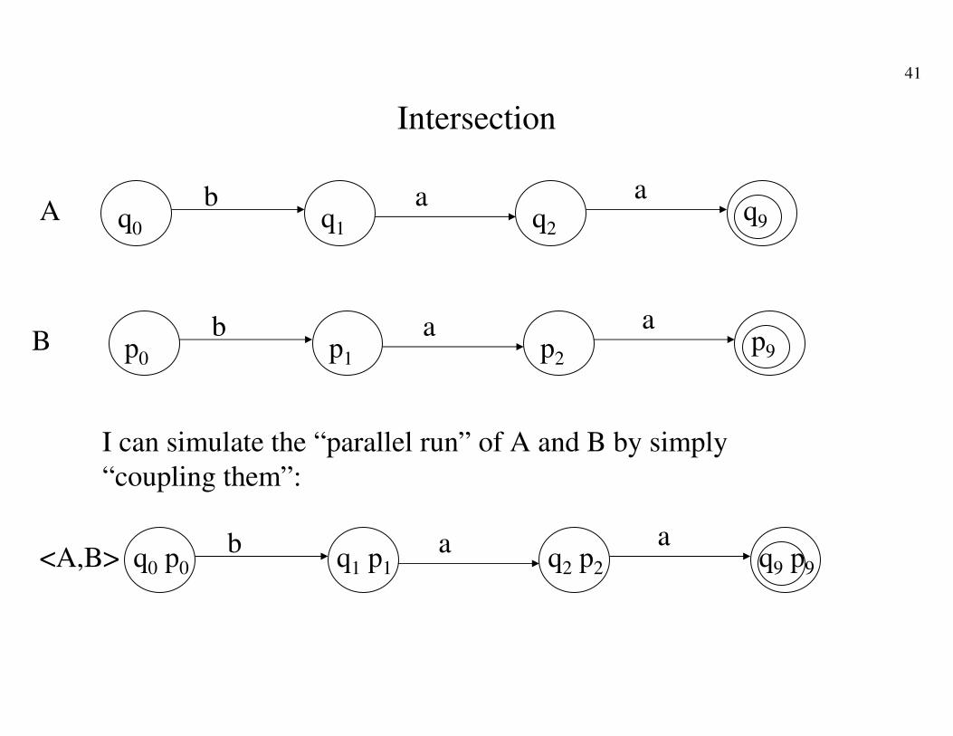
Intersection
a abq1 q2q0
q9
a abp1 p2
p0
p9
A
B
I can simulate the “parallel run” of A and B by simply
“coupling them”:
a abq0<A,B> p1q1 p2q2 p9q9
p0
42
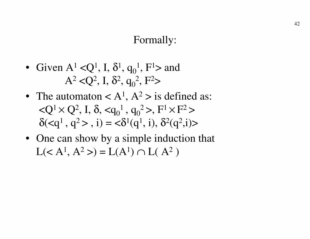
Formally:
• Given A1 <Q1, I, δ1, q01, F1> and
A2 <Q2, I, δ2, q02, F2>
• The automaton < A1, A2 > is defined as:
<Q1 × Q2, I, δ, <q01 , q0
2 >, F1 × F2 >
δ(<q1 , q2 > , i) = <δ1(q1, i), δ2(q2,i)>
• One can show by a simple induction that
L(< A1, A2 >) = L(A1) ∩ L( A2 )

43
Union
• A similar construction …
otherwise ... exploit identity A ∪ B = ¬(¬A ∩ ¬B)
⇒ need a FSA for the complement language
Complement:
q0 q1
10 0
1
An idea: F^ = Q - F:
Yes, it works for the automaton above, but ….
44
q0 q1
10 0
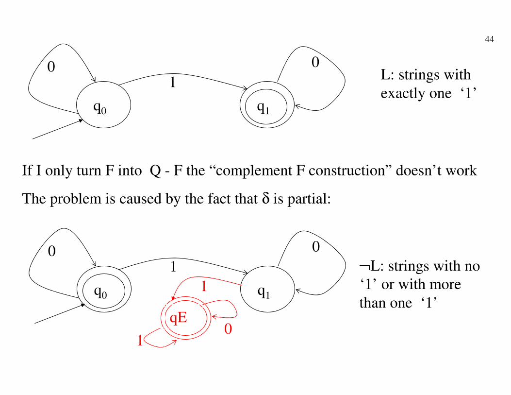
If I only turn F into Q - F the “complement F construction” doesn’t work
The problem is caused by the fact that δ is partial:
q0 q1
10 0
qE0
1
1
L: strings with
exactly one ‘1’
¬L: strings with no ‘1’ or with more
than one ‘1’
45
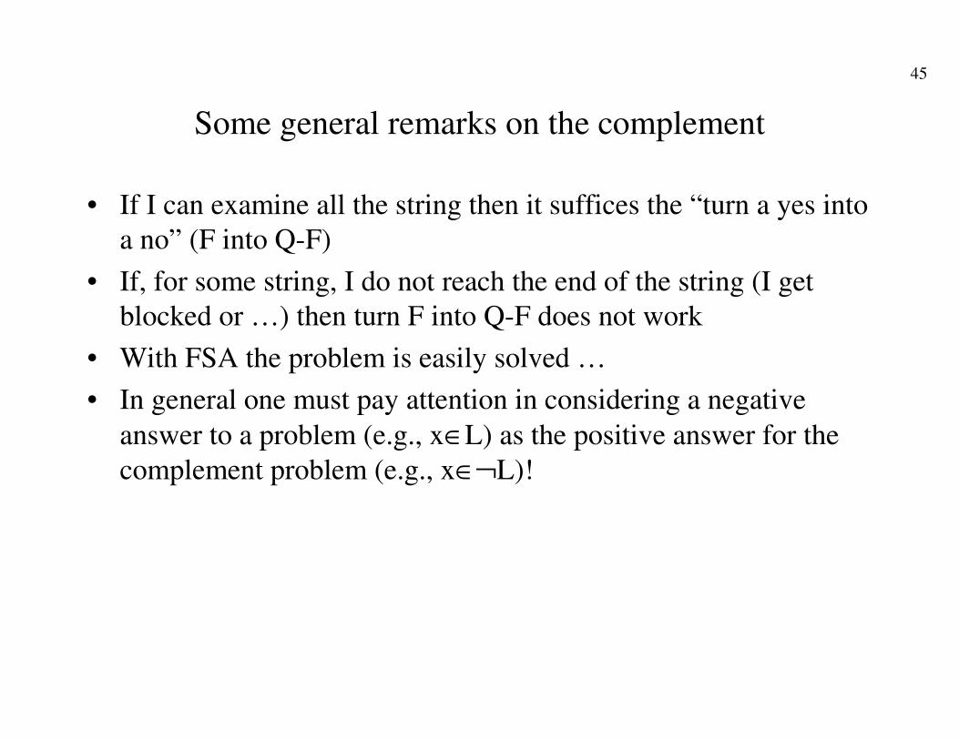
Some general remarks on the complement
• If I can examine all the string then it suffices the “turn a yes into
a no” (F into Q-F)
• If, for some string, I do not reach the end of the string (I get
blocked or …) then turn F into Q-F does not work
• With FSA the problem is easily solved …
• In general one must pay attention in considering a negative
answer to a problem (e.g., x∈L) as the positive answer for the
complement problem (e.g., x∈¬L)!

46
Let us increase the power of the FSA
by increasing its memory
• A more “mechanical” view of the FSA:
Input tape
Output tape
Control device
(finite state)

47
• Now let us “enrich it” :
Input tape
Output tape
Control device
(finite state)
x
a
A
pq
B
Z0
“stack” memory

48
The move of the stack automaton:
• Depending on :
– the symbol read on the input tape (but it could also not read anything …)
– the symbol read on top of the stack
– the state of the control device:
• the stack automaton
– changes its state
– moves ahead the scanning head
– changes the symbol A read on top of the stack with a string α of
symbols (possibly empty: this amounts to a pop of A)
– (if translator) it writes a string (possibly empty) on the output tape
(moving the writing head consequently)

49
• The input string x is recognized (accepted) if
– The automaton scans it completely (the scanning head
reaches the end of x)
– Upon reaching the end of x it is in an acceptance state (just
like for the FSA)
• If the automaton is also a translator, then
τ(x) is the string on the output tape after x has been
completely scanned (if x is accepted, otherwise τ(x) is
undefined: τ(x) = ⊥
(⊥ is the “undefined” symbol)

50
A first example: accepting {anbn | n > 0}
q0 q3
a,A/AA
a,Z0/ Z0 B
b,A/ε
b,A/ε
b,B /ε
q2q1
a,B/BA
Z0
B
A
A } n - 1 A’s
b,B /ε
the B in the stack marks
the first symbol of x, to
match the last symbol
51
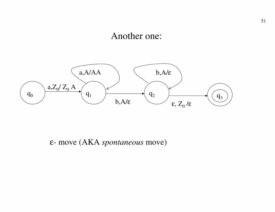
Another one:
q0 q3
a,A/AA
a,Z0/ Z0 A
b,A/ε
b,A/ε
ε, Z0 /ε
q2q1
ε- move (AKA spontaneous move)
52
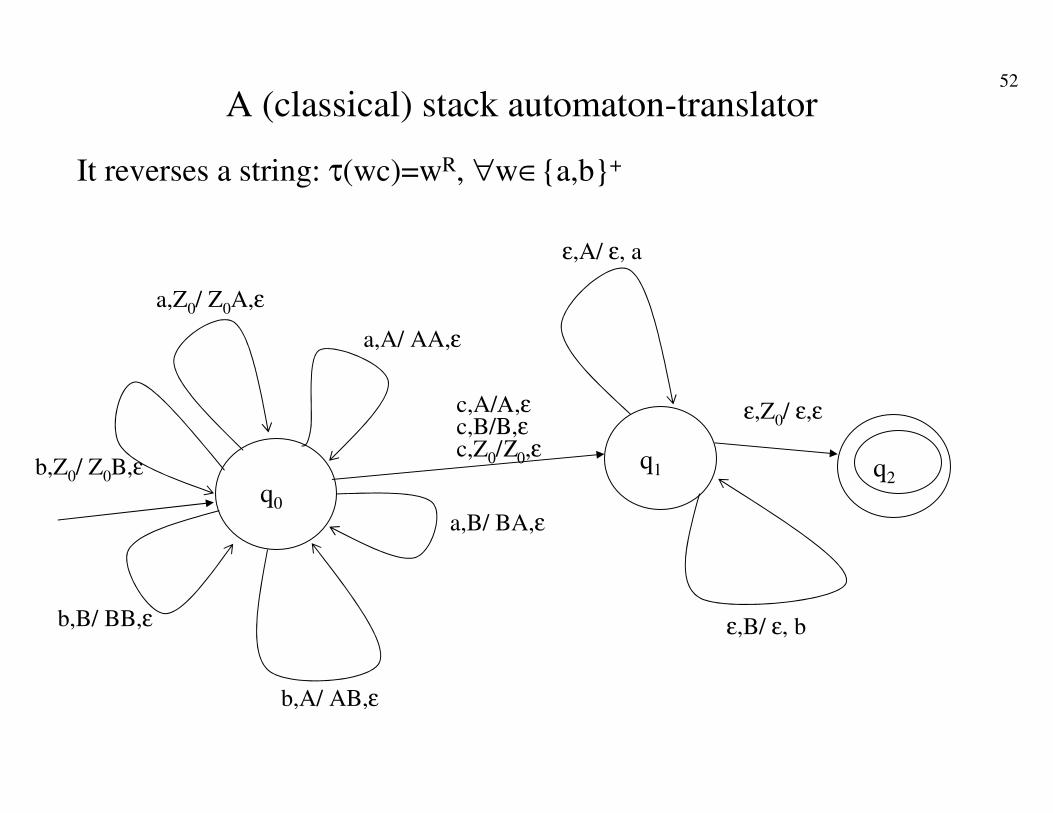
A (classical) stack automaton-translator
a,Z0/ Z0A,ε
a,A/ AA,ε
a,B/ BA,ε
b,Z0/ Z0B,ε
b,A/ AB,ε
b,B/ BB,ε
ε,A/ ε, a
ε,B/ ε, b
ε,Z0/ ε,ε
q0
q1 q2
It reverses a string: τ(wc)=wR, ∀w∈{a,b}+
c,A/Α,εc,B/Β,εc,Z0/Ζ0,ε

53
Now we formalize ...
• Stack automaton [transducer]: <Q,I,Γ,δ, q0, Z0 , F [, O, η]>
• Q, I, q0, F [O] just like FSA [FST]
• Γ stack alphabet (disjoint from other ones for ease of definition)
• Z0 : initial stack symbol (not essential, useful to simplify definitions)
• δ: Q × (I ∪ {ε}) × Γ → Q × Γ* δ : partial!
• η: Q × (I ∪ {ε}) × Γ → O* ( η defined where δ is)
Graphical notation:
i,A/α,w
q p
<p,α> = δ(q,i, A)
w = η(q,i, A)

54
• Configuration (a generalization of the notion of state):
c = <q, x, γ, [z]>:
– q: state of the control device
– x: unread portion of the input string (the head is positioned
on the first symbol of x)
– γ : string of symbols in the stack(convention: <high-right, low-left>)
– z: string written (up to now) on the output tape
55
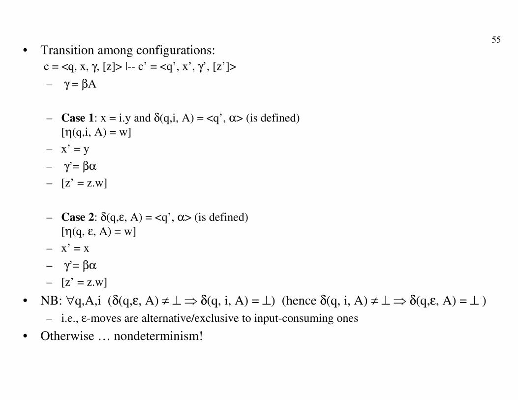
• Transition among configurations:
c = <q, x, γ, [z]> |-- c’ = <q’, x’, γ’, [z’]>
– γ = βA
– Case 1: x = i.y and δ(q,i, A) = <q’, α> (is defined)
[η(q,i, A) = w]
– x’ = y
– γ’= βα
– [z’ = z.w]
– Case 2: δ(q,ε, A) = <q’, α> (is defined)
[η(q, ε, A) = w]
– x’ = x
– γ’= βα
– [z’ = z.w]
• NB: ∀q,A,i (δ(q,ε, A) ≠ ⊥ ⇒ δ(q, i, A) = ⊥) (hence δ(q, i, A) ≠ ⊥ ⇒ δ(q,ε, A) = ⊥ )
– i.e., ε-moves are alternative/exclusive to input-consuming ones
• Otherwise … nondeterminism!
56
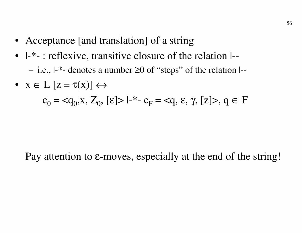
• Acceptance [and translation] of a string
• |-*- : reflexive, transitive closure of the relation |--
– i.e., |-*- denotes a number ≥0 of “steps” of the relation |--
• x ∈ L [z = τ(x)] ↔
c0 = <q0,x, Z0, [ε]> |-*- cF = <q, ε, γ, [z]>, q ∈ F
Pay attention to ε-moves, especially at the end of the string!

57
Stack automata in practice
• They are the heart of compilers
• Stack memory (LIFO) suitable to analyze nested
syntactic structures (arithmetical expressions,
compound instructions, …)
• Abstract run-time machine for programming languages
with recursion
• ….
Will occur very frequently in the course of Languages
and translators

58Properties of stack automata
(especially as acceptors)
• {anbn | n > 0} is accepted by a stack automaton (not by a FSA)
– However {anbncn | n > 0} ….
– NOT: after counting –using the stack- n a’s and “de-counting” n b’s howcan we remember n to count the c’s?The stact is a destructive memory: to read it, one must destroy it!This limitation of the stack automaton can be proved formally through a generalization of the pumping lemma.
• {anbn | n > 0} accepted by a stack automaton;{anb2n | n > 0} accepted by a stack automaton
• However {anbn | n > 0} ∪ {anb2n | n > 0} …
– Reasoning -intuitively- similar to the previous one:
– If I empty all the stack with n b’s then I forget if there are other b’s
– If I empty only half the stack and I do not find any more b I cannot knowif I am halfway in the stack
– The formalization of this reasoning is however not trivial ….

59
Some consequences
• LP = class languages accepted by stack automata
• LP is not closed under union nor intersection
• Why?
– [consider the languages {anbncn | n > 0} and {anbn | n > 0} ∪ {anb2n | n > 0} ]
• Considering the complement …
The same principle as with FSA: change the accepting states
into non accepting states.
There are however new difficulties
60
• Function δ must be completed (as with FSA) with an error state.
Pay attention to the nondeterminism caused by ε-moves!
• The ε-moves can cause cycles ---> never reach the end of the string ----> the string is not accepted, but it is not accepted either
by the automaton with F^ = Q-F.
• There exists however a construction that associates to every
automaton an equivalent loop-free automaton
• Not finished yet: what if there is a sequence of ε-moves at the end of the scanning with some states in F and other ones not in
F?

61
• <q1, ε, γ1> |-- <q2, ε, γ2> |-- <q3, ε, γ3> |-- …
q1∈ F, q2 ∉ F, …. ?
• Then we must “force” the automaton to accept only at the end of a
(necessarily finite) sequence of ε-moves.
• This is also possible through a suitable construction.
Once more, rather than the technicalities of the construction/proof we are
interested in the general mechanism to accept the complement of a language:
sometimes the same machine that solves the “positive instance” of the
problem can be adapted to solve the “negative instance”: this can be trivial or
difficult: we must be sure to be able to complete the construction
62
Stack automata [as acceptors (SA) or translators (ST)] are more
powerful than finite state ones (a FSA is a trivial special case of a SA;
more, SA have an unlimited counting ability that FSA lack)
However also SA/ST have their limitations …
… a new and “last” (for us) automaton:
the Turing Machine (TM)
Historical model of “computer”, simple and conceptually important
under many aspects.
We consider it as an automaton; then we will derive from it some
important, universal properties of automatic computation.
For now we consider the “K-tape” version, slightly different than the
(even simpler) original model. This choice will be explained later.
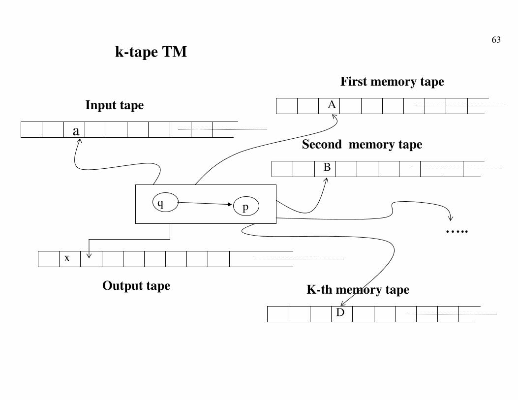
63
Input tape
Output tape
x
a
pq
k-tape TM
First memory tape
A
Second memory tape
B
K-th memory tape
D
…..

64
Informal Description and Partial Formalization of the TM
• States and alphabets as with other automata (input, output, control device, memory
alphabet)
• For historical reasons and due to some “mathematical technicalities” the tapes are
represented as infinite cell sequences [0,1,2, …] rather than finite strings. There
exists however a special symbol “blank” (“ ”, or “barred b” or “_”) and it is
assumed that every tape contains only a finite number of non-blank cells.
– The equivalence of the two ways of representing the tape content is obvious.
• Scanning and output heads are also as in previous models

65
• The move of the TM:
• Reading:– one symbol on the input tape
– k symbols on the k memory tapes
– state of the control device
• Action:– State change: q ----> q’
– Write a symbol in place of the one read on each of the k memory tapes: Ai ----> Ai’, 1 <= i <= k
– [Write a symbol on the output tape]
– Move of the k + 2 heads:• memory and scanning heads can move one position right (R) or left (L) or
stand still (S)
• The output head can move one position right (R) or stand still (S) (if it has written it moves; if it moves without writing it leaves a blank on the tape cell)
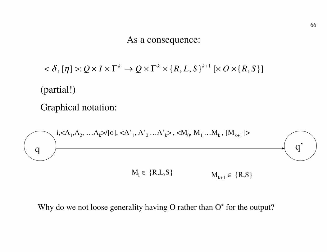
66
As a consequence:
}],{[},,{:][, 1SROSLRQIQ
kkk ×××Γ×→Γ××>< +ηδ
(partial!)
Graphical notation:
q q’
i,<A1,A2, …Ak>/[o], <A’1, A’2 …A’k> , <M0, M1 …Mk , [Mk+1 ]>
Mi ∈ {R,L,S}
Why do we not loose generality having O rather than O* for the output?
Mk+1 ∈ {R,S}

67
• Initial configuration:
•Z0 followed by all blanks in the memory tapes
•[output tape all blank]
•Heads in the 0-th position on every tape
•Initial state of the control device q0
•Input string x starting from the 0-th cell of the input tape,
followed by all blanks
68
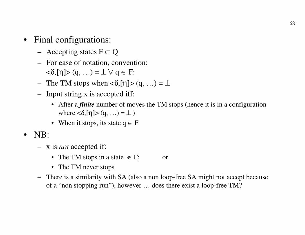
• Final configurations:
– Accepting states F ⊆ Q
– For ease of notation, convention:
<δ,[η]> (q, …) = ⊥ ∀ q ∈ F:
– The TM stops when <δ,[η]> (q, …) = ⊥
– Input string x is accepted iff:
• After a finite number of moves the TM stops (hence it is in a configuration
where <δ,[η]> (q, …) = ⊥ )
• When it stops, its state q ∈ F
• NB:
– x is not accepted if:
• The TM stops in a state ∉ F; or
• The TM never stops
– There is a similarity with SA (also a non loop-free SA might not accept because
of a “non stopping run”), however … does there exist a loop-free TM?

69
Some examples
• A TM accepting {anbncn | n > 0}
Input tape
aMemory tape
M
aa b bb c cc
MMZ0
CD

70
a, Z0/Z0, <S, R>
q0 q1
a, _ / M, <R, R>
q2
b, _ / _, <S, L>
b, M / M, <R, L>
q3
c, Z0/Z0, <S, R>
c, M / M, <R, R>
qF
_, _ / _, <S, S>

71
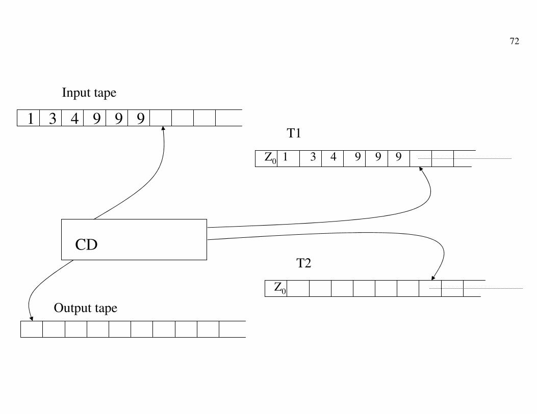
Computing the successor of a number n coded with decimal digits
two memory tapes T1 and T2
• M copies all digits of n on T1, to the right of Z0, while it moves head T2 by the same number of positions.
• M scans the digits of T1 from right to left. It writes on T2 fromright to left changing the digits as needed (9’s become 0’s, first digit≠9 becomes the successive digit, then all other ones are unchanged, …)
• M copies T2 on the output tape.
• Notation: � : any decimal digit
• _ : blank
• # : any digit ≠ 9
• ^ : successor of a digit denoted as # (in the same transition)
72
Input tape
3T1
41 9 99
41Z0
CDT2
Z0
3 9 9 9
Output tape

73
q0 q1 q2
q3 q4
q5
q6 q7
�,Z0,Z0/_,<Z0,Z0>,<S,R,R,S>
�,_,_/_,< �,_>,<R,R,R,S>
_,_,_/_,< _,_>,<S,L,L,S>
_,9,_/_,< 9,0>,
<S,L,L,S>
_,#,_/_,< #,^>,<S,L,L,S>_, �,_/_,< �, � >,<S,L,L,S>
_,Z0,Z0/_,<Z0,Z0>,<S,R,R,S>
_, �, � / �,< �, � >,<S,R,R,R>_,_,_/_,< _,_>,<S,S,S,S>
_,Z0,Z0/1,<Z0,Z0>,<S,R,R,R>
_, �, 0 / 0,< �, 0 >,<S,R,R,R>
_,_,_/_,< _,_>,<S,S,S,S>
left end reached (all
9’s): add an initial 1
then all others are 0
copy input on T1 Change rightmost 9’s into 0’s
copy all T2 on outputcopy rest of T1 on T2
74
Closure properties of TM
• ∩ : OK (a TM can easily simulate two other ones, both “in series” and “in parallel”)
• ∪ : OK (idem)• Idem for other operations (concatenation, *, ….)
• What about the complement?
Negative answer! (Proof later on)If there existed loop-free TM’s, it would be easy: it would suffice to define the set of halting states (it is easy to make it disjoint from the set of non-halting states) and partition it into accepting and non-accepting states.
==========>It is therefore apparent that the problem arises from nonterminating computations

75
Equivalent TM models
• Single tape TM (NB: ≠ TM with 1 –memory! – tape)
A single tape (usually unlimited in both directions):
serves as input, memory, and output
CD
x
76
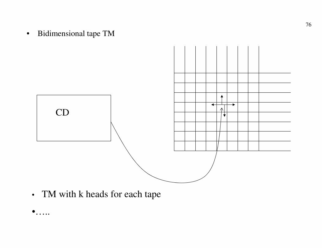
• Bidimensional tape TM
CD
• TM with k heads for each tape
•…..
77
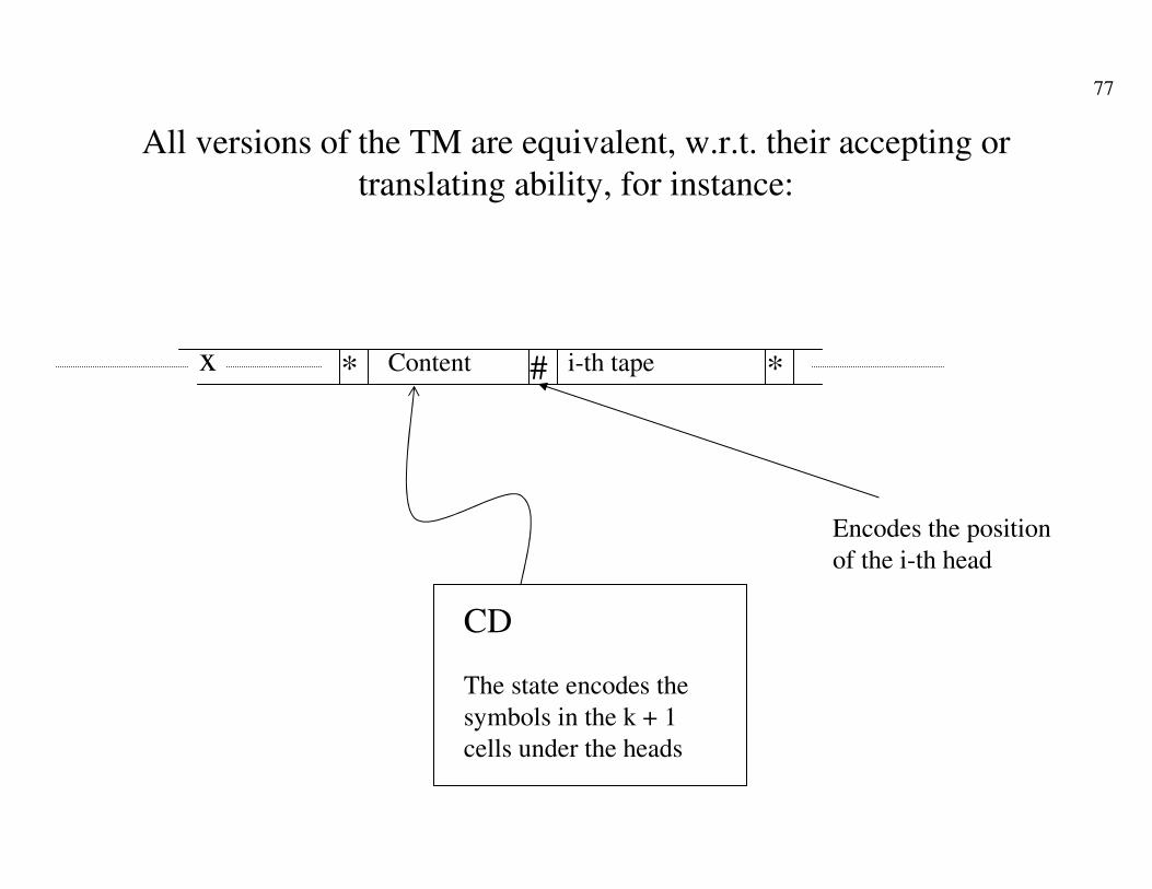
All versions of the TM are equivalent, w.r.t. their accepting or
translating ability, for instance:
CD
x * Content i-th tape *#
Encodes the position
of the i-th head
The state encodes the
symbols in the k + 1
cells under the heads

78
What relations exist among the various automata (TM in
particular) and more traditional/realistic computing models?
•The TM can simulate a Von Neumann machine (which is also “abstract”)
•The main difference is in the way the memory is accessed: sequential rather than
“random” (direct)
•This does not influence the machine for what concerns computational power (i.e., the
class of problem it can solve)
•There can be a (profound) impact for what concerns the complexity of the
computations
• We will consider the implications in both cases
79
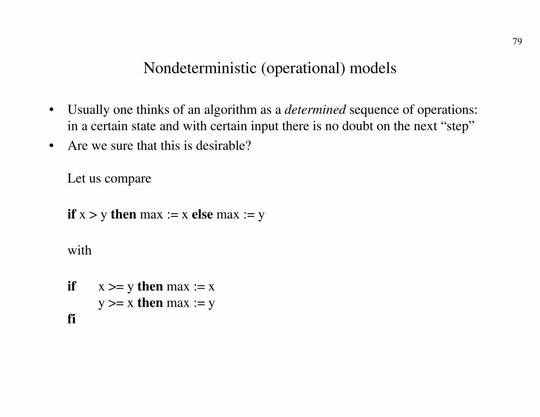
Nondeterministic (operational) models
• Usually one thinks of an algorithm as a determined sequence of operations:
in a certain state and with certain input there is no doubt on the next “step”
• Are we sure that this is desirable?
Let us compare
if x > y then max := x else max := y
with
if x >= y then max := x
y >= x then max := y
fi

80
• Is it only a matter of elegance?
• Let us consider the case construct of Pascal & others:
why not having something like the following?
case
– x = y then S1
– z > y +3 then S2
– …. then …
endcase

81
Another form of nondeterminism which is usually “hidden”:
blind search
?

82
• In fact, the search algorithms are a “simulation” of “basically
nondeterministic” algorithms:
• Is the searched element in the root of the tree?
• If yes, OK. Otherwise
– Search the left subtree
or
– Search the right subtree
• Choice of priority among various paths is often arbitrary
• If we were able to assign to tasks in parallel to two distinct machines ---->
• Nondeterminism as a model of computation or at least a model of design of
parallel computing
(For instance Ada and other concurrent languages exploit the
nondeterminism)
83
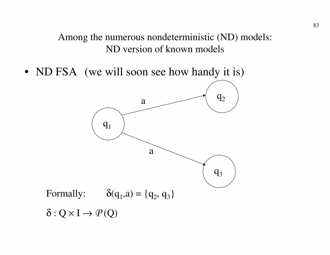
Among the numerous nondeterministic (ND) models:
ND version of known models
• ND FSA (we will soon see how handy it is)
q1
q2
q3
a
a
Formally: δ(q1,a) = {q2, q3}
δ : Q × I → P (Q)
84
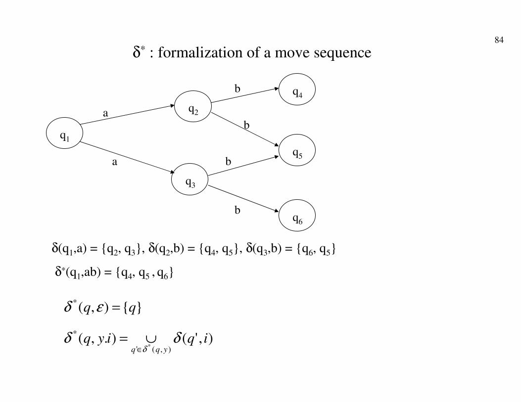
δ* : formalization of a move sequence
q1
q2
q3
a
a
q4
q5
q6
b
b
b
b
δ(q1,a) = {q2, q3}, δ(q2,b) = {q4, q5}, δ(q3,b) = {q6, q5}
δ∗(q1,ab) = {q4, q5 , q6}
),'().,(
}{),(
),('
*
*
*iqiyq
yqqδδ
εδ
δ∈∪=
=
85
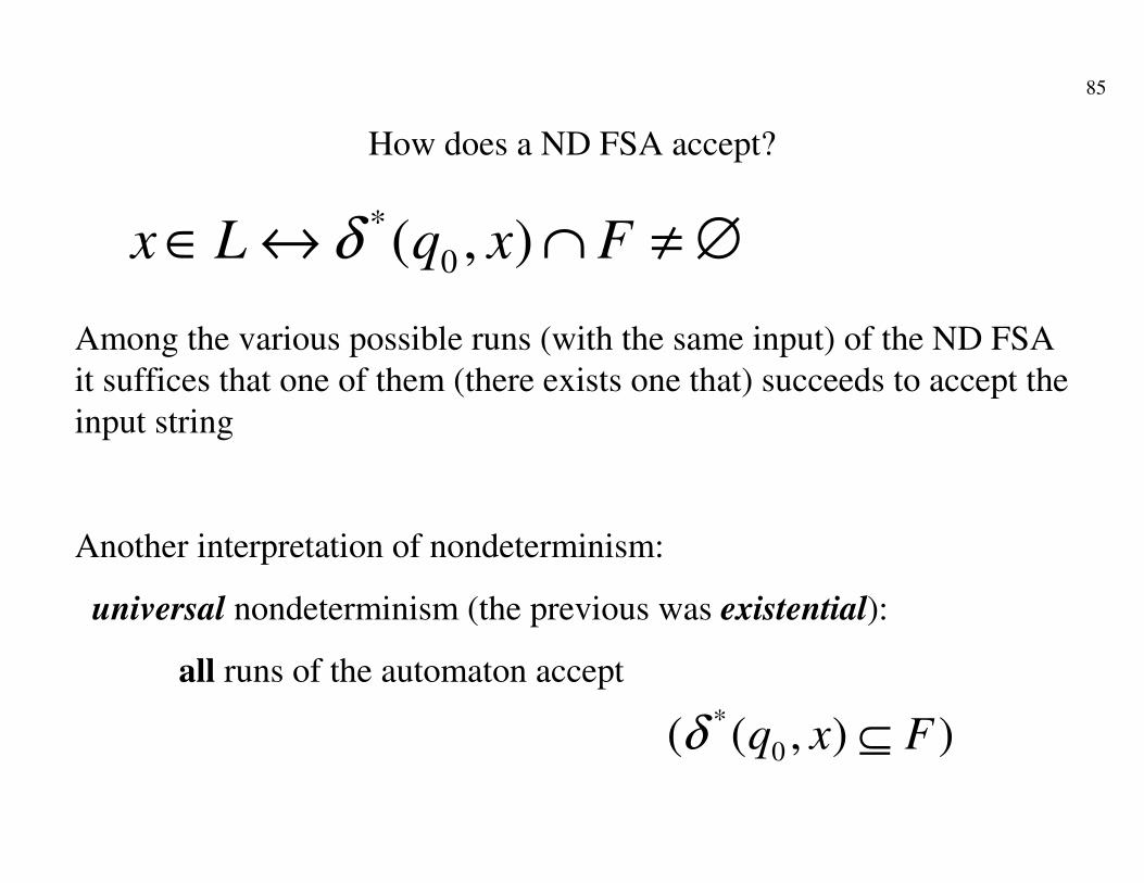
How does a ND FSA accept?
∅≠∩↔∈ FxqLx ),( 0
*δ
Among the various possible runs (with the same input) of the ND FSA
it suffices that one of them (there exists one that) succeeds to accept the
input string
Another interpretation of nondeterminism:
universal nondeterminism (the previous was existential):
all runs of the automaton accept
)),(( 0
*Fxq ⊆δ
86
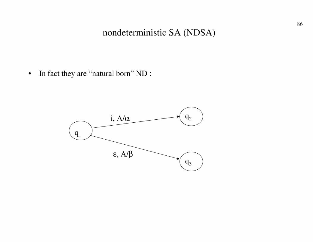
nondeterministic SA (NDSA)
• In fact they are “natural born” ND :
q1
q2
q3
i, A/α
ε, A/β

87
• Why index F? (finite subset)
• As usual, the NDSA accepts x if there exists a sequence
• c0 |-*- <q, ε, γ>, q ∈ F
• |-- is not unique (i.e., functional) any more!
)(}){(: *Γ×℘→Γ×∪× QIQ Fεδ
• We might as well remove the deterministic constraint and generalize:
q1
q2
q3
i, A/α
i, A/β

88
A “trivial” example: accepting {anbn | n>0} ∪{anb2n | n>0}
q0’ q3’
a,A/AA
a,Z0/ Z0 A
b,A/ε
b,A/ε
ε, Z0 /εq2’q1’
q0” q4
a,A/AA
a,Z0/ Z0 A
b,A/Α
b,A/εε, Z0 /ε
q2q1
b,A/Α
q3
q0
ε,Z0/ Z0
ε,Z0/ Z0
89
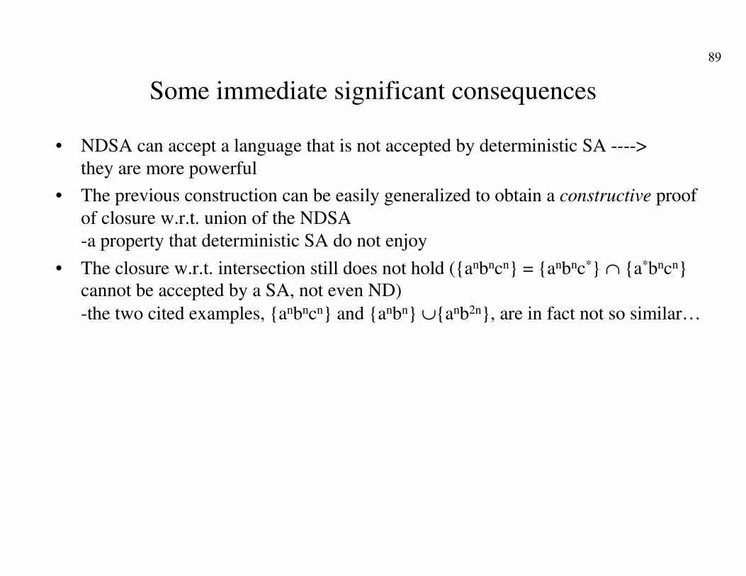
Some immediate significant consequences
• NDSA can accept a language that is not accepted by deterministic SA ---->
they are more powerful
• The previous construction can be easily generalized to obtain a constructive proof
of closure w.r.t. union of the NDSA
-a property that deterministic SA do not enjoy
• The closure w.r.t. intersection still does not hold ({anbncn} = {anbnc*} ∩ {a*bncn} cannot be accepted by a SA, not even ND)
-the two cited examples, {anbncn} and {anbn} ∪{anb2n}, are in fact not so similar…
90
• If a language family is closed w.r.t. union and not w.r.t. intersection
it cannot be closed w.r.t. complement (why?)
• Hence languages NDSA are not closed w.r.t. complement
• This highlights a deep change caused by nondeterminism concerning the
complement of a problem -in general-:
if the way of operating of a machine is deterministic and its computation
finishes it suffices to change the positive answer into a negative one to obtain
the solution of the “complement problem” (for instance, presence rather than
absence of errors in a program)

91
• In the case of NDSA, though it is possible, like for DSA, to make a
computation always finish, there can be two computations
– co |-*- <q1, ε, γ1>
– co |-*- <q2, ε, γ2>
– q1 ∈ F, q2 ∉ F
• In this case x is accepted
• However, if F turned into Q-F, x is still accepted:
with nondeterminism changing a yes into a no does not work!
• And other kinds of automata?
92
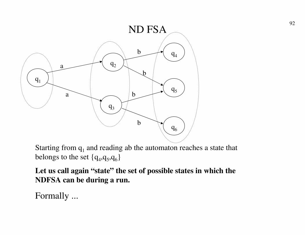
ND FSA
q1
q2
q3
a
a
q4
q5
q6
b
b
b
b
Starting from q1 and reading ab the automaton reaches a state that
belongs to the set {q4,q5,q6}
Let us call again “state” the set of possible states in which the
NDFSA can be during a run.
Formally ...
93
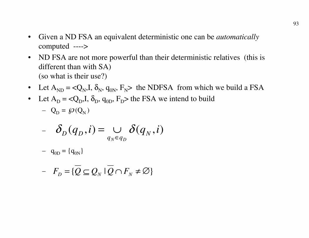
• Given a ND FSA an equivalent deterministic one can be automatically
computed ---->
• ND FSA are not more powerful than their deterministic relatives (this is
different than with SA)
(so what is their use?)
• Let AND = <QN,I, δN, q0N, FN> the NDFSA from which we build a FSA
• Let AD = <QD,I, δD, q0D, FD> the FSA we intend to build
– QD = ℘(QN )
–
– q0D = {q0N}
–
),(),( iqiq Nqq
DDDN
δδ∈∪=
}|{ ∅≠∩⊆= NND FQQQF

94
• Though it is true that for all NDFSA one can find (and build) an equivalent
deterministic one
• This does not mean that using NDFSA is useless:
– It can be easier to “design” a NDFSA and then obtain from it automatically an
equivalent deterministic one, just to skip the (painful) job of build it ourselves
deterministic from the beginning (we will soon see an application of this idea)
– For instance, from a NDFSA with 5 states one can obtain, in the worst case, one
with 25 states!
• Consider NFA and DFA for languages L1=(a,b)*a(a,b) (i.e., strings over
{a,b} with ‘a’ as the symbol before the last one) and L2=(a,b)*a(a,b)4 (i.e., ‘a’
as the fourth symbol before the last...)
• We still have to consider the TM ...

95
Nondeterministic TM
}]),{[},,{(:][, 1 SROSLRQIQ kkk ×××Γ×℘→Γ××>< +ηδ
•Is the index F necessary?
•Configurations, transitions, transition sequences and acceptance
are defined as usual
•Does nondeterminism increment the power of TM’s?

96
Computation tree
c32
c0
c22c21
c13c12c11
c26c25c23 c24
c31 ckjcim
C accepting
C halt but not
accepting
Unfinished
computations

97
• x is accepted by a ND TM iff there exists a computation that terminates in an
accepting state
• Can a deterministic TM establish whether a “sister” ND TM accepts x, that is,
accept x if and only if the ND TM accepts?
• This amounts to “visit” the computation tree of the NDTM to establish
whether it contains a path that finishes in an accepting state
• This is a (almost) trivial, well known problem of tree visit, for which there are
classical algorithms
• The problem is therefore reduced to implementing an algorithm for visiting
trees through TM’s: a boring, but certainly feasible exercise … but beware the
above “almost” ...

98
• Everything is easy if the computation tree is finite
• But it could be that some paths of the tree are infinite (they describe
nonterminating computations)
• In this case a depth-first visit algorithm (for instance leftmost preorder) might
“get stuck in an infinite path” without ever discover that another branch is
finite and leads to the acceptance.
• The problem can however be easily overcome by adopting, for instance, a
breadth-first visit algorithm (it uses a queue data structure rather than a stack
to manage the nodes still to be visited).
• Hence nondeterminism does not increase the power of the TM
99
Conclusions
• Nondeterminism: a useful abstraction to describe search problems and algorithms; situations
where there are no elements of choice or they are equivalent, or parallel computations
• In general it does not increase the computing power, at least in the case of TM’s (which are the
most powerful automaton seen so far) but it can provide more compact descriptions
• It increases the power of stack automata
• It can be applied to various computational models (to every one, in practice); in some cases
“intrinsically nondeterministic” models were invented to describe nondeterministic phenomena
• For simplicity we focused only on (D and ND) acceptors but the notion applies also to
translator automata.
• NB: the notion of ND must not be confused with that of stochastic (there exist stochastic
models -e.g. Markov chains- that are completely different from the nondeterministic ones)
100
Grammars
• Automata are a model suitable to recognize/accept, translate, compute
(languages): they “receive” an input string and process it in various ways
• Let us now consider a generative model:
a grammar produces, or generates, strings (of a language)
• General notion of a grammar or syntax (mathematically, alphabet and
vocabulary, and grammar and syntax are synonymous):
set of rules to build phrases of a language (strings): it applies to any notion of
a language in the widest possible sense.
• In a way similar to normal linguistic mechanisms a formal grammar
generates strings of a language through a process of rewriting:

101
• “A phrase is made of a subject followed by a predicate”
“A subject can be a noun or a pronoun, or …”
“A predicate can be a verb followed by a complement…”
• A program consists of a declarative part and an executable part
The declarative part …
The executable part consists of an statement sequence
A statement can be simple or compound
….
102
• An email message consists of a header and a bodyThe header contains an address, ….
• …
• In general this kind of linguistic rules describes a “main object” (a book, a program, a message, a protocol, ….) as a sequence of “composing objects”(subject, header, declarative part, …). Each of these is then “refined” by replacing it with more detailed objects and so on, until a sequence of base elements is obtained (bits, characters, …)The various rewriting operations can be alternative: a subject can be a noun or a pronoun or something else; a statement can be an assignment, or I/O, ...
103
Formal definition of a grammar
• G = <VN, VT, P, S>
– VN : nonterminal alphabet or vocabulary
– VT : terminal alphabet or vocabulary
– V = VN ∪ VT
– S ∈ VN : a particular element of VN called axiom or initial
symbol
– : set of rewriting rules, or productions.*VVP N ×⊆ +
}{ ritenotation w of easefor },{ βαβα →=><= PP
104
Example
• VN = {S, A, B, C, D}
• VT = {a,b,c}
• S
• P = {S → AB, BA → cCD, CBS → ab, A → ε}

105
Immediate derivation Relation
><
∈→∧==
↔
∈∈⇒+
3122
22321321
*
, ofcontext in the asrewritten is
,
,,
ααβα
βααβαβααα
βαβα
Pa
VV
With reference to the previous grammar:
aaBAS ⇒ aacCDS
As usual, define the reflexive and transitive closure of ⇒:
⇒*

106
Language generated by a grammar
}|{)(*
* xSVxxGL T ⇒∧∈=
Consists of all strings, containing only terminal symbols, that can be
derived (in any number of steps) from S
NB: not all derivations lead to a string of terminal symbols
some may “get stuck”

107
A first example
0.},{)(
:tiongeneralizaeasy an Through
0
0
0
0
sderivation Some
}0,,,,{
,},0,,{},,,{
*
1
1
bbaaGL
aabbaabbSaabBaaSaAS
bbbbSbBS
aaaaSaAS
S
SbSBbBSaSAaASP
SPbaBASG
=
⇒⇒⇒⇒⇒
⇒⇒⇒
⇒⇒⇒
⇒
→→→→→=
>=<

108
Second example
}0|{)(
obtain we with production ngsubstitutiBy
}1|{)(
:tiongeneralizaeasy an Through
sderivation Some
),for on abbreviati(}|{
,},,{},{
2
2
2
≥=
→→
≥=
⇒⇒⇒
⇒⇒
⇒
→→→=
>=<
nbaGL
SabS
nbaGL
aaabbbaaSbbaSbS
aabbaSbS
abS
abSaSbSabaSbSP
SPbaSG
nn
nn
ε
109
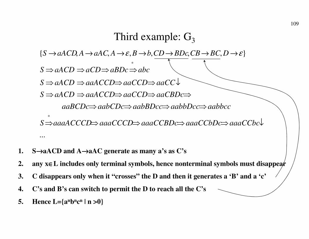
Third example: G3
...
},,,,,,{
*
*
↓⇒⇒⇒⇒⇒
⇒⇒⇒⇒
⇒⇒⇒⇒⇒
↓⇒⇒⇒⇒
⇒⇒⇒⇒
→→→→→→→
aaaCCbcaaaCCbDcaaaCCBDcaaaCCCDaaaACCCDS
aabbccaabbDccaabBDccaabCDcaaBCDc
aaCBDcaaCCDaaACCDaACDS
aaCCaaCCDaaACCDaACDS
abcaBDcaCDaACDS
DBCCBBDcCDbBAaACAaACDS εε
1. S→→→→aACD and A→→→→aAC generate as many a’s as C’s
2. any x∈∈∈∈L includes only terminal symbols, hence nonterminal symbols must disappear
3. C disappears only when it “crosses” the D and then it generates a ‘B’ and a ‘c’
4. C’s and B’s can switch to permit the D to reach all the C’s
5. Hence L={anbncn | n >0}

110
Some “natural” questions
• What is the practical use of grammars (beyond funny
“tricks” like {anbn}?)
• What languages can be obtained through grammars?
• What relations exist among grammars and automata
(better: among languages generated by grammars and
languages accepted by automata?

111
Some answers
• Definition of the syntax of the programming languages
• Applications are “dual” w.r.t. automata
• Simplest example: language compilation: the grammar
defines the language, the automaton accepts and
translates it.
• More systematically:

112
Classes of grammars
• Context-free grammars:
– ∀ α → β ∈ P, |α| = 1, i.e., α is an element of VN.
– Context free because the rewriting of α does not depend on its context (part of the string surrounding it).
– These are in fact the same as the BNF used for defining the
syntax of programming languages (so they are well fit to
define typical features of programming and natural
languages, … but not all)
– G1 e G2 above are context-free not so for G3.
113
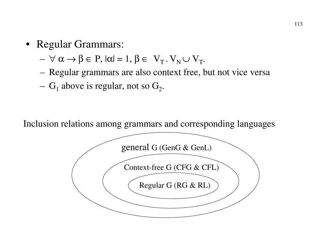
• Regular Grammars:
– ∀ α → β ∈ P, |α| = 1, β ∈ VT . VN ∪ VT.
– Regular grammars are also context free, but not vice versa
– G1 above is regular, not so G2.
Inclusion relations among grammars and corresponding languages
general G (GenG & GenL)
Context-free G (CFG & CFL)
Regular G (RG & RL)
114
It immediately follows that :
RL ⊆ CFL ⊆ GenL
But, are inclusions strict?
The answer comes from the comparison with automata
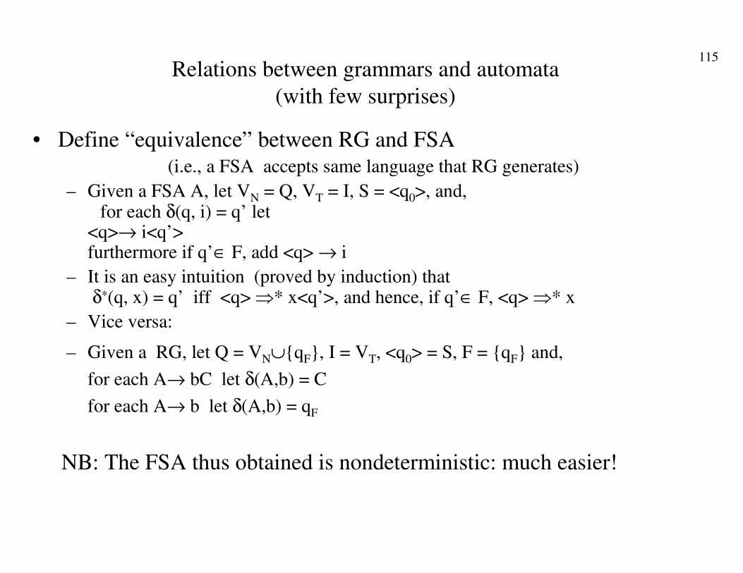
115Relations between grammars and automata
(with few surprises)
• Define “equivalence” between RG and FSA (i.e., a FSA accepts same language that RG generates)
– Given a FSA A, let VN = Q, VT = I, S = <q0>, and, for each δ(q, i) = q’ let
<q>→ i<q’>furthermore if q’∈ F, add <q> → i
– It is an easy intuition (proved by induction) thatδ∗(q, x) = q’ iff <q> ⇒* x<q’>, and hence, if q’∈ F, <q> ⇒* x
– Vice versa:
– Given a RG, let Q = VN∪{qF}, I = VT, <q0> = S, F = {qF} and,
for each A→ bC let δ(A,b) = C
for each A→ b let δ(A,b) = qF
NB: The FSA thus obtained is nondeterministic: much easier!

116
• CFG equivalent to SA (ND!)
intuitive justification (no proof:
the proof is the “hart” of compiler construction)
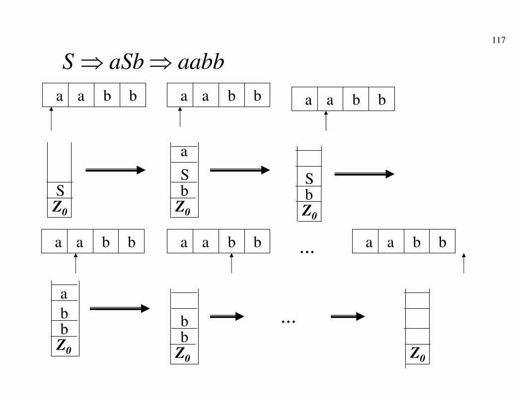
117
aabbaSbS ⇒⇒
a a b b
S
a a b b
bS
a
a a b b
bS
a a b b
bb
a
a a b b
bb
a a b b
Z0 Z0 Z0
Z0 Z0 Z0
…
…

118
genG equivalent to TM
• Given G let us construct (in broad lines) a ND TM, M,
accepting L(G):
– M has one memory tape
– The input string x is on the input tape
– The memory tape is initialized with S (better: Z0S)
– The memory tape (which, in general, will contain a string α,
α ∈ V*) is scanned searching the left part of some production of P
– When one is found -not necessarily the first one, M operates
a ND choice- it is substituted by the corresponding right part
(if there are many right parts again M operates
nondeterministically)
119
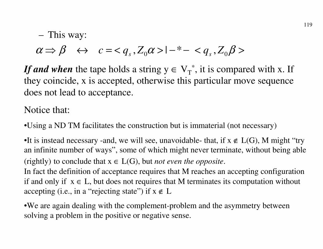
– This way:
><−−><=↔⇒ βαβα 00 ,*|, ZqZqc ss
If and when the tape holds a string y ∈ VT*, it is compared with x. If
they coincide, x is accepted, otherwise this particular move sequence
does not lead to acceptance.
Notice that:
•Using a ND TM facilitates the construction but is immaterial (not necessary)
•It is instead necessary -and, we will see, unavoidable- that, if x ∉ L(G), M might “try an infinite number of ways”, some of which might never terminate, without being able
(rightly) to conclude that x ∈ L(G), but not even the opposite.
In fact the definition of acceptance requires that M reaches an accepting configuration
if and only if x ∈ L, but does not requires that M terminates its computation without
accepting (i.e., in a “rejecting state”) if x ∉ L
•We are again dealing with the complement-problem and the asymmetry between
solving a problem in the positive or negative sense.

120
• Given M (single tape, for ease of reasoning and without loss
of generality) let us build (in broad lines) a G, that generates
L(M):
– First, G generates all strings of the type
x$X, x ∈ VT*, X being a “copy of x” composed of nonterminal
symbols (e.g., for x = aba, x$X = aba$ABA)
– G simulates the successive configurations of M using the string on
the right of $
– G is defined in a way such that it has a derivation x$X ⇒* x if and only if x is accepted by M.
– The base idea is to simulate each move of M by an immediate
derivation of G:

121
– We represent the configuration
q
α A βCB
• through the string (special cases are left as an exercise): $αBqACβ
• G has therefore derivations of the kind x$X⇒x$qoX (initial configuration of M)
• If, for M it is defined :
– δ(q,A) = <q’, A’, R> G includes the production qA → A’q’
– δ(q,A) = <q’, A’, S> G includes the production qA → q’ A’
– δ(q,A) = <q’, A’, L> G includes the production BqA → q’ BA’
∀ B in the alphabet of M (recall that M is single tape, hence it has a unique alphabet for input, memory, and output)
122
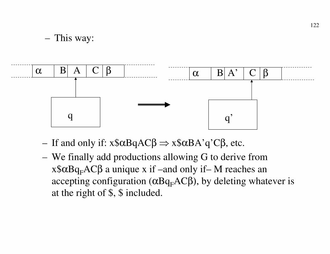
– This way:
q
α A βCB
q’
α A’ βCB
– If and only if: x$αBqACβ ⇒ x$αBA’q’Cβ, etc.
– We finally add productions allowing G to derive from
x$αBqFACβ a unique x if –and only if– M reaches an
accepting configuration (αBqFACβ), by deleting whatever is at the right of $, $ included.