Earth-Science Reviews 150 (2015) 201–218

Contents lists available at ScienceDirect

Earth-Science Reviews

j ourna l homepage: www.e lsev ie r .com/ locate /earsc i rev

Theoretical foundation of cyclostationary EOF analysis for geophysicaland climatic variables: Concepts and examples

Kwang-Yul Kim a,⁎, Benjamin Hamlington b, Hanna Na c

a School of Earth and Environmental Sciences, Seoul National University, Seoul, Republic of Koreab Department of Ocean, Earth and Atmospheric Research, Old Dominion University, Norfolk, USAc Faculty of Science, Hokkaido University, Japan

⁎ Corresponding author at: School of Earth and EnvironUniversity, Seoul 151-742, Republic of Korea.

E-mail address: kwang56@snu.ac.kr (K.-Y. Kim).

http://dx.doi.org/10.1016/j.earscirev.2015.06.0030012-8252/© 2015 The Authors. Published by Elsevier B.V

a b s t r a c t

a r t i c l e i n f o

Article history:Received 14 January 2015Received in revised form 11 May 2015Accepted 9 June 2015Available online 29 July 2015

Keywords:Space-time eigen analysisData analysisPhysical and dynamical modes

Natural variability is an essential component of observations of all geophysical and climate variables. In principalcomponent analysis (PCA), also called empirical orthogonal function (EOF) analysis, a set of orthogonaleigenfunctions is found from a spatial covariance function. These empirical basis functions often lend useful in-sights into physical processes in the data and serve as a useful tool for developing statistical methods. The under-lying assumption in PCA is the stationarity of the data analyzed; that is, the covariance function does not dependon the origin of time. The stationarity assumption is often not justifiable for geophysical and climate variableseven after removing such cyclic components as the diurnal cycle or the annual cycle. As a result, physical and sta-tistical inferences based on EOFs can be misleading.Some geophysical and climatic variables exhibit periodically time-dependent covariance statistics. Such a datasetis said to be periodically correlated or cyclostationary. A proper recognition of the time-dependent response char-acteristics is vital in accurately extracting physically meaningful modes and their space–time evolutions fromdata. This also has important implications in finding physically consistent evolutions and teleconnection patternsand in spectral analysis of variability—important goals inmany climate and geophysical studies. In this study, theconceptual foundation of cyclostationary EOF (CSEOF) analysis is examined as an alternative to regular EOF anal-ysis or other eigenanalysis techniques based on the stationarity assumption. Comparative examples and illustra-tions are given to elucidate the conceptual difference between the CSEOF technique and other techniques and theentailing ramification in physical and statistical inferences based on computational eigenfunctions.

© 2015 The Authors. Published by Elsevier B.V. This is an open access article under the CC BY-NC-ND license(http://creativecommons.org/licenses/by-nc-nd/4.0/).

Contents

1. Introduction . . . . . . . . . . . . . . . . . . . . . . . . . . . . . . . . . . . . . . . . . . . . . . . . . . . . . . . . . . . . . 2012. Cyclostationary EOF analysis . . . . . . . . . . . . . . . . . . . . . . . . . . . . . . . . . . . . . . . . . . . . . . . . . . . . . . 2033. Nested periodicity . . . . . . . . . . . . . . . . . . . . . . . . . . . . . . . . . . . . . . . . . . . . . . . . . . . . . . . . . . . 2044. A simple example of CSEOF analysis . . . . . . . . . . . . . . . . . . . . . . . . . . . . . . . . . . . . . . . . . . . . . . . . . . . 2055. Implications on physical inferences . . . . . . . . . . . . . . . . . . . . . . . . . . . . . . . . . . . . . . . . . . . . . . . . . . . 2066. Implications on spectral inferences . . . . . . . . . . . . . . . . . . . . . . . . . . . . . . . . . . . . . . . . . . . . . . . . . . . 2117. Utility of CSEOF analysis . . . . . . . . . . . . . . . . . . . . . . . . . . . . . . . . . . . . . . . . . . . . . . . . . . . . . . . . 2128. Concluding remarks . . . . . . . . . . . . . . . . . . . . . . . . . . . . . . . . . . . . . . . . . . . . . . . . . . . . . . . . . . 216Acknowledgments . . . . . . . . . . . . . . . . . . . . . . . . . . . . . . . . . . . . . . . . . . . . . . . . . . . . . . . . . . . . . 217Appendix 1. A comparison between CSEOF analysis and extended EOF analysis . . . . . . . . . . . . . . . . . . . . . . . . . . . . . . . . 217References . . . . . . . . . . . . . . . . . . . . . . . . . . . . . . . . . . . . . . . . . . . . . . . . . . . . . . . . . . . . . . . . . 217

mental Sciences, Seoul National

. This is an open access article under

1. Introduction

Measurements of physical and climate variables show the presenceof seemingly random fluctuations in addition to such deterministiccomponents as the diurnal cycle and the annual cycle. This random

the CC BY-NC-ND license (http://creativecommons.org/licenses/by-nc-nd/4.0/).

Fig. 1. Monthly variance of the NINO3 time series after removing the monthly meanvalues.

202 K.-Y. Kim et al. / Earth-Science Reviews 150 (2015) 201–218

component of variability is often referred to as natural variability asopposed to “forced variation” in the presence of external forcing to aphysical system. Natural variability has been the focus of numerousstudies not only because it is an essential concept in addressing climateand environmental changes due to such external forcing agents asgreenhouse gasses (Jones et al., 1994; Andreae et al., 2005) or volcanicaerosols (Rampino and Self, 1992; Zielinski et al., 1996; Jones et al.,2005) but also because natural variability is important on its own accord(Luterbacher et al., 2004; Bengtsson et al., 2006; Swanson et al., 2009).Much national and international effort focuses on the study of naturalvariability in understanding the current and future climate changes(NAC, 1995; IPCC, 2007, 2013).

The stochastic component of variability is often treated as a randomvariable. This does not mean that the source of random fluctuation istruly and solely the random nature of our physical and climate systems;this rather reflects our incomplete comprehension of how the systemworks in its full detail. Such a notion is often reflected in our attemptsto assign physical meaning to seemingly stochastic undulations ofsome physical and climate variables. It may be fair to say that thestudy of natural variability in many applications is best approached bytreating it as a random variable. Thus, data analysis often deals withmultivariate random variables in space and time.

A random variable cannot be described in a deterministic manner. Itcan only be described in terms of probability, p(X), of a random variableX having values in an event space A, i.e., X∈ A. The event space is a sub-set of sample space, Ω, which represents a collection of all possiblevalues of X. A probability density function (pdf) is often awkward touse and is also difficult to estimate accurately from limited observation-al datasets. Thus, themoment statistics of randomvariables are comput-ed instead in a simplified approach. The nth moment is defined as

E Xn� � ¼Z

Ωxnp xð Þdx ¼ Xn� �

; ð1Þ

where x is a particular realization of the random variable X, E(•) is the ex-pectation, and ⟨•⟩ represents ensemble averaging. Having all of themoment statistics of a random variable is equivalent to knowing its pdf.The attractiveness of the moment statistics over the pdf lies in the alter-native way of computing the former as suggested in Eq. (1)—namely,ensemble averaging without invoking a true pdf.

Typically, it is assumed that a random variable, T(x), is reasonablydescribed in terms of its first twomoment statistics, i.e., themean func-tion and the covariance function:

μ xð Þ ¼Z

ΩT xð Þp T xð Þð ÞdT ¼ T xð Þh i; ð2Þ

C x; x′� � ¼

ZΩT ′ xð Þp T ′ xð Þ

� �T ′ x′� �

p T ′ x′� �� �

dT ′ ¼ T ′ xð ÞT ′ x′� �D E

; ð3Þ

where T′(x) = T(x)− μ(x) and independent variable x represents time,space, or both. According to the independent variable, the covariancefunction, C(x, x′), may be called a temporal, spatial or spatio-temporalcovariance function. Thus, the computation and analysis of the firsttwo moment statistics of a given dataset constitute an essential step ofanalyzing random variables.

Computation of the two moment statistics in Eqs. (2) and (3) maylook simple, but it actually is difficult because we do not know the pdfnor do we usually have enough realizations for ensemble averaging. Ingeophysical studies, we typically have only one realization (one obser-vational record) for a physical variable of interest because we cancarry out only one experiment (one Earth). Modeling studies, of course,can provide us with as many realizations as we want. The veracity ofmodel statistics, on the other hand, should be tested against the statis-tics of observational data. Thus, it is necessary to introduce a simplifyingassumption to find the first two moment statistics of observed data.

An assumption we often introduce in analyzing a random variable isstationarity. The essence of this assumption is that themoment statisticsof a random variable are independent of time. When this assumptionapplies to the first two moment statistics, such a random variable iscalled “weakly” stationary. What is implicit in Eqs. (2) and (3) is thatT(x) and T(x′) are different random variables since their statistics, ingeneral, are different. Under the stationarity assumption, however, thetwo random variables at two different times x and x′ have the samestatistics and, henceforth, are regarded the same. Thus, T(x) and T(x′)may be viewed as two different realizations of the random variable T.As a result, the ensemble average in Eqs. (2) and (3) can be replacedby averaging in the time direction:

μ ¼ T tð Þh i ¼ limN→∞

1N

XN

t¼1T tð Þ; ð4Þ

C t; t ′� � ¼ T ′ tð ÞT ′ t ′

� �D E¼ lim

N→∞

1N

XN

t¼1T ′ tð ÞT ′ t þ τð Þ ¼ R τð Þ; ð5Þ

where τ = t − t′ corresponds to lag and N is the number of samples.Here, the independent variable, time t, has been introduced explicitly.Note that C(t, t′) is no longer a function of time because of the station-arity assumption but depends only on lag τ. The function R(τ) is calledthe autocovariance function, meaning the covariance function of thesame variable (self). In a similar manner, a spatial covariance functioncan be constructed as

C x; x′� � ¼ T x; tð ÞT x′; t

� �� � ¼ limN→∞

1N

XN

t¼1T x; tð ÞT x′; t

� �; ð6Þ

where T(x, t) hereafter denotes a zero-mean random variable and x is aspatial independent variable. One can, of course, extend the definitionfurther to define a space–time covariance function:

C x; t; x′; t ′� � ¼ T x; tð ÞT x′; t ′

� �� � ¼ limN→∞

1N

XN

t¼1T x; tð ÞT x′; t þ τ

� �: ð7Þ

Mainly because of the difficulty involved in the computation of Eq. (7),rarely seen in geophysical research is the analysis of a spatio-temporalcovariance function.

While the stationarity assumption allows us to carry out the seem-ingly impossible calculations in Eqs. (2) and (3) from a limited dataset,statistics ofmany geophysical variables unfortunately do not exhibit thestationary behavior. Instead, many geophysical variables have statisticsthat are time dependent and periodic (see Section 6 in Gardner et al.(2006) and references therein). For example, the monthly variance ofthe NINO3 time series is strongly time dependent as shown in Fig. 1;NINO3 is a region in the equatorial Pacific defined by [150°–90°W,5°S–5°N]. While there is no significant time-dependent component inthe insolation statistics after removing the annual cycle, Fig. 1 showsthat the variability of the equatorial climate system is stronger inwinter

203K.-Y. Kim et al. / Earth-Science Reviews 150 (2015) 201–218

than in summer. This time dependence of statistics is a prevalent prop-erty of many geophysical variables. This raises two important concerns:(1) many statistical tools based on the stationarity assumption will notbe accurate thereby leading to inaccurate statistical inferences; and(2) statistical tools should be developed that explicitly account for thistime dependence. The second concern is difficult to address in that thedevelopment of general data analysis techniques for nonstationaryspace–time data would be nearly impossible.

In addition to the time dependence, statistics of many geophysicalvariables exhibit periodicity in time. Such a process is said to becyclostationary or periodically correlated. The periodicity of statisticsmay primarily come from the periodic nature of external forcing andboundary conditions associated with our climate and geophysical sys-tems although they may not necessarily be an exclusive source of peri-odicity in the statistics. With this added assumption of periodicity, thesecond concern raised above can be dealt with efficiently as will beshown later. It is this special class of data forwhich amore accurate con-cept of data analysis will be discussed.

It should be stressed that the periodic nature of our physical systemmanifests itself not only in the mean field, such as the annual cycle andthe diurnal cycle, but also in higher-moment statistics. The periodicmean component of data does not pose any problem since it can beidentified and removed prior to analysis. The periodic components inhigher-moment statistics, however, are difficult to deal with. For sim-plicity, let us confine our discussion to the second-moment statistics.

The time dependence of variance statistics such as shown in Fig. 1can be eliminated by using the so-called variance normalization or sta-bilization procedure. This procedure is summarized as

Tnorm tð Þ ¼ T tð Þσ tð Þ ; ð8Þ

where raw data, T(t), are divided by the respective standard deviation,σ(t), at each time step t. Then, the variance of the resulting time serieswill be uniform in time. This procedure, however, does not alter thecorrelation structure between two different times. As shown in Fig. 2,lagged correlation function of the NINO3 time series remains to betime dependent even after the variance normalization procedure is ap-plied. There is also an interesting asymmetry between positive and neg-ative lags in the correlation structure. This asymmetry also varies intime. Thus, time dependence of covariance statistics should be dealtwith explicitly; there is no circumventing this fundamental structureof the second-moment statistics.

The second-moment statistics are often recast in different forms in-cluding the spectral density function and EOFs. An EOF analysis repre-sents decomposition of the second-moment statistics in space (spatial

Fig. 2. Lagged correlation, C(t, τ) = ⟨T(t)T(t + τ)⟩, of the NINO3 time series, where theordinate denotes t and the abscissa τ (month). A positive lag refers to a future time withrespect to the reference time t. The NINO3 time series has been variance normalized bydividing eachmonthly value by the respective month's standard deviation after removingthe monthly mean values.

covariance function) into computational orthogonal functions, whichwill be discussed below in detail. The spectral density function is aFourier transformation of the autocovariance function, and is conceptual-ly equivalent to an EOF analysis in the time domain. This pointwill also beaddressed in more detail in Section 6. The lack of stationarity in the tem-poral statistics of many geophysical variables means that statistical infer-ences made through the two very popular techniques—spectral analysisand EOF analysis—are subject to potentially serious faults. The discussionbelow elaborates on this point and, as an alternate method, CSEOF analy-sis is introduced. The conceptual foundation of the technique is explainedwith illustrations and examples in comparison with the EOF techniqueand also with the extended EOF and complex EOF techniques as needed.Computational algorithms for the CSEOF technique have been publishedelsewhere (Kim et al., 1996; Kim and North, 1997b) and will not bediscussed in this paper.

2. Cyclostationary EOF analysis

Themodal decomposition in terms of a set of basis functions is oftenuseful in understanding the complicated response in a physical system.The complicated response is decomposed into less complicated basicpatterns, which, in general, may be easier to understand and shedmore insight into the nature of variability in a given physical system.Many theoretical basis functions have been studied extensively in thecontext of the Sturm–Liouville problem (Richtmyer, 1978; Arfken andWeber, 1995). Unfortunately, exact theoretical basis functions are verydifficult to find, since our physical and climate systems are extremelycomplicated. Therefore, empirical basis functions (EOFs) are soughtinstead (Jolliffe, 2002; Hannachi et al., 2007). Finding computationalbasis functions are further complicated if the stationarity assumptionis abandoned.

Let us consider a simple temporally discrete physical systemdefinedby

T x; tð Þ ¼ B x; tð ÞS tð Þ; ð9Þ

where B(x, t) is a physical processmodulated by a stochastic time seriesS(t). Then, it can be shown that

μ x; tð Þ ¼ T x; tð Þh i¼ B x; tð Þ S tð Þh i ¼ B x; tð ÞμS;

ð10Þ

C x; t; x′; t ′� � ¼ T x; tð ÞT x′; t ′

� �� �¼ B x; tð ÞB x′; t ′

� �S tð ÞS t ′

� �� � ¼ B x; tð ÞB x′; t ′� �

RS τð Þ; ð11Þ

where μS and RS(τ) are themean and the autocovariance function of thepurely stochastic component, S(t), respectively. Thus, the first two mo-ment statistics are shown to be time dependent in the presence of atime-dependent physical process, B(x, t). Further, the time dependenceof the statistics comes, in theory, only from the physical component notfrom the stochastic component of data in Eq. (9).

There are ample examples from geophysical observations suggest-ing that physical processes, and, henceforth, corresponding statistics,are time dependent. This can be seen, for example, in the covariancefunction, C(t, t′), of the NINO3 time series (Fig. 3). As shown, there is aprominent time dependence in the covariance statistics. Such a time-dependent structure cannot come from stationary random fluctuations.This should be contrasted with the stationarity assumption, underwhich

C t; t ′� � ¼ R t−t ′

� � ¼ R τð Þ: ð12Þ

In other words, covariance statistics of a stationary time series do notdepend on time; they depend only on lag, τ. Note specifically in EOFanalysis that physical response characteristics of a physical process areassumed to be stationary and not dependent on time in EOF analysis.

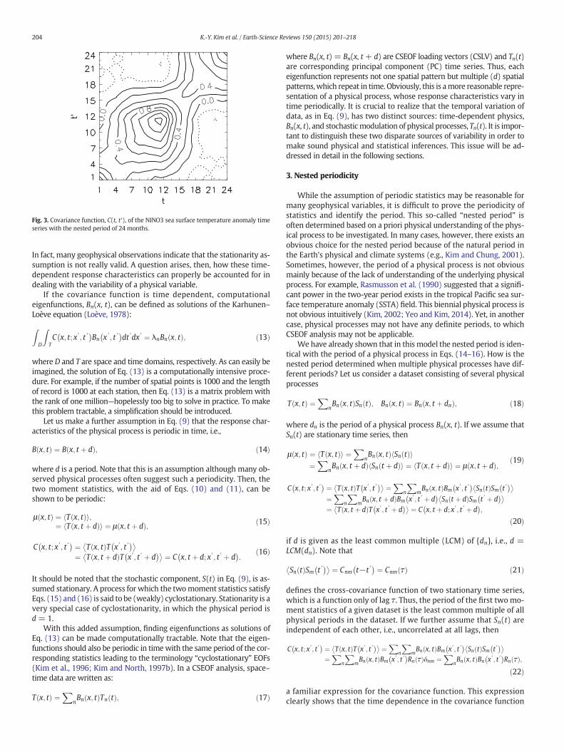
Fig. 3. Covariance function, C(t, t′), of the NINO3 sea surface temperature anomaly timeseries with the nested period of 24 months.

204 K.-Y. Kim et al. / Earth-Science Reviews 150 (2015) 201–218

In fact, many geophysical observations indicate that the stationarity as-sumption is not really valid. A question arises, then, how these time-dependent response characteristics can properly be accounted for indealing with the variability of a physical variable.

If the covariance function is time dependent, computationaleigenfunctions, Bn(x, t), can be defined as solutions of the Karhunen–Loève equation (Loève, 1978):

ZD

ZTC x; t; x′; t ′� �

Bn x ′; t ′� �

dt ′dx′ ¼ λnBn x; tð Þ; ð13Þ

where D and T are space and time domains, respectively. As can easily beimagined, the solution of Eq. (13) is a computationally intensive proce-dure. For example, if the number of spatial points is 1000 and the lengthof record is 1000 at each station, then Eq. (13) is a matrix problem withthe rank of one million—hopelessly too big to solve in practice. To makethis problem tractable, a simplification should be introduced.

Let us make a further assumption in Eq. (9) that the response char-acteristics of the physical process is periodic in time, i.e.,

B x; tð Þ ¼ B x; t þ dð Þ; ð14Þ

where d is a period. Note that this is an assumption although many ob-served physical processes often suggest such a periodicity. Then, thetwo moment statistics, with the aid of Eqs. (10) and (11), can beshown to be periodic:

μ x; tð Þ ¼ T x; tð Þh i;¼ T x; t þ dð Þh i ¼ μ x; t þ dð Þ; ð15Þ

C x; t; x′; t ′� � ¼ T x; tð ÞT x′; t ′

� �� �¼ T x; t þ dð ÞT x′; t ′ þ d

� �� � ¼ C x; t þ d; x′; t ′ þ d� �

:ð16Þ

It should be noted that the stochastic component, S(t) in Eq. (9), is as-sumed stationary. A process for which the twomoment statistics satisfyEqs. (15) and (16) is said to be (weakly) cyclostationary. Stationarity is avery special case of cyclostationarity, in which the physical period isd = 1.

With this added assumption, finding eigenfunctions as solutions ofEq. (13) can be made computationally tractable. Note that the eigen-functions should also be periodic in timewith the same period of the cor-responding statistics leading to the terminology “cyclostationary” EOFs(Kim et al., 1996; Kim and North, 1997b). In a CSEOF analysis, space–time data are written as:

T x; tð Þ ¼X

nBn x; tð ÞTn tð Þ; ð17Þ

where Bn(x, t) = Bn(x, t+ d) are CSEOF loading vectors (CSLV) and Tn(t)are corresponding principal component (PC) time series. Thus, eacheigenfunction represents not one spatial pattern but multiple (d) spatialpatterns,which repeat in time. Obviously, this is amore reasonable repre-sentation of a physical process, whose response characteristics vary intime periodically. It is crucial to realize that the temporal variation ofdata, as in Eq. (9), has two distinct sources: time-dependent physics,Bn(x, t), and stochasticmodulation of physical processes, Tn(t). It is impor-tant to distinguish these two disparate sources of variability in order tomake sound physical and statistical inferences. This issue will be ad-dressed in detail in the following sections.

3. Nested periodicity

While the assumption of periodic statistics may be reasonable formany geophysical variables, it is difficult to prove the periodicity ofstatistics and identify the period. This so-called “nested period” isoften determined based on a priori physical understanding of the phys-ical process to be investigated. In many cases, however, there exists anobvious choice for the nested period because of the natural period inthe Earth's physical and climate systems (e.g., Kim and Chung, 2001).Sometimes, however, the period of a physical process is not obviousmainly because of the lack of understanding of the underlying physicalprocess. For example, Rasmusson et al. (1990) suggested that a signifi-cant power in the two-year period exists in the tropical Pacific sea sur-face temperature anomaly (SSTA) field. This biennial physical process isnot obvious intuitively (Kim, 2002; Yeo and Kim, 2014). Yet, in anothercase, physical processes may not have any definite periods, to whichCSEOF analysis may not be applicable.

We have already shown that in this model the nested period is iden-tical with the period of a physical process in Eqs. (14–16). How is thenested period determined when multiple physical processes have dif-ferent periods? Let us consider a dataset consisting of several physicalprocesses

T x; tð Þ ¼X

nBn x; tð ÞSn tð Þ; Bn x; tð Þ ¼ Bn x; t þ dnð Þ; ð18Þ

where dn is the period of a physical process Bn(x, t). If we assume thatSn(t) are stationary time series, then

μ x; tð Þ ¼ T x; tð Þh i ¼X

nBn x; tð Þ Sn tð Þh i

¼X

nBn x; t þ dð Þ Sn t þ dð Þh i ¼ T x; t þ dð Þh i ¼ μ x; t þ dð Þ; ð19Þ

C x; t; x′; t ′� � ¼ T x; tð ÞT x′; t ′

� �� � ¼ Xn

XmBn x; tð ÞBm x′; t ′

� �Sn tð ÞSm t ′

� �� �¼

Xn

XmBn x; t þ dð ÞBm x′; t ′ þ d

� �Sn t þ dð ÞSm t ′ þ d

� �� �¼ T x; t þ dð ÞT x′; t ′ þ d

� �� � ¼ C x; t þ d; x′; t ′ þ d� �

;

ð20Þ

if d is given as the least common multiple (LCM) of {dn}, i.e., d =LCM(dn). Note that

Sn tð ÞSm t ′� �� � ¼ Cnm t−t ′

� � ¼ Cnm τð Þ ð21Þ

defines the cross-covariance function of two stationary time series,which is a function only of lag τ. Thus, the period of the first two mo-ment statistics of a given dataset is the least common multiple of allphysical periods in the dataset. If we further assume that Sn(t) areindependent of each other, i.e., uncorrelated at all lags, then

C x; t; x′; t ′� � ¼ T x; tð ÞT x′; t ′

� �� � ¼ Xn

XmBn x; tð ÞBm x′; t ′

� �Sn tð ÞSm t ′

� �� �¼

Xn

XmBn x; tð ÞBm x′; t ′

� �Rn τð Þδnm ¼

XnBn x; tð ÞBn x′; t ′

� �Rn τð Þ;ð22Þ

a familiar expression for the covariance function. This expressionclearly shows that the time dependence in the covariance function

205K.-Y. Kim et al. / Earth-Science Reviews 150 (2015) 201–218

comes only from the physical evolutions constituting the datasetand signifies the motivation of the CSEOF technique—physical de-composition of variability. Note that Rn(τ) in Eq. (22) does not con-tribute to the temporal covariance structure but only affects themagnitude of the covariance function.

The consequence of d being the LCM of all physical periods is thatphysical processes with a period less than d are shown to repeat incyclostationary loading vectors, Bn(r, t). For example, a physical processwith a period of 6 monthswill repeat twice in the corresponding CSEOFloading vectors if d is set to 12 months. Although the nested period canbe set to be an integral multiple of the LCM of all physical periods, theminimum period should be used; this is to minimize the contaminationof covariance statistics by sampling errors. Typically, one has to workwith a relatively short record so that the stationarity of the stochasticcomponents in Eqs. (19) and (20) is difficult to establish. This contami-nates the estimation of covariance statistics, which, in turn, distortsphysical structures in CSEOF loading vectors.

4. A simple example of CSEOF analysis

Fig. 4 shows the first CSEOF with the nested period of 12 months ofthe tropical Pacific sea surface temperatures (SST). The PC time seriesindicates that the first CSEOF presents the annual cycle; the amplitudeis always positive indicating that the loading patterns appear everyyear without any sign change. Unlike a conventional analysis such ascomposite analysis or harmonic analysis, the amplitude of the annual

Fig. 4. The first CSEOF of the monthly sea surface temperatures in the tropical

cycle is not a constant; it fluctuates interannually. The spatial loadingpatterns depict the evolution of the tropical Pacific sea surface temper-ature in the annual cycle. As addressed above, the loading patternsdescribe the evolution of a physical process called the annual cyclewhereas the PC time series describes the “stochastic” amplitude varia-tion of the annual cycle.

Fig. 5 shows the first two EOFs of the tropical Pacific SST. The firstEOF resembles the March and September patterns and the second EOFthe June and December patterns of the first CSEOF. Undoubtedly, thefirst two EOFs capture the characteristic features of the annual cycle.The corresponding time series are highly correlated (correlation =0.75) at 3-month lag with the second PC time series leading the firstPC time series. This is consistent with the interpretation of the spatialpatterns in the context of the annual cycle.

Fig. 6 shows the loading vector of the second CSEOF mode of thetropical Pacific SST and represents El Niño; the loading patterns looksimilar to the second EOF pattern. Indeed, the two PC time series arehighly correlated (correlation = 0.60), and the 1982/1983 and 1997/1998 El Niño events are captured in both the time series. This is clearlya serious problem, since the second EOFmode reflects both the seasonalcycle and the El Niño. An identical evolution pattern in two or more dis-tinct physical processes is captured as a single EOFmode, and this leadsto an ambiguous physical and statistical inference.

Fig. 7 shows the evolution of equatorial SST in the first CSEOF andthat in the first two extended EOFs (EEOFs; see Appendix 1 for thedefinition of EEOFs) in comparison with the monthly composite (see

Pacific (upper panel) and the corresponding PC time series (lower panel).

Fig. 5. The first two EOF modes of the monthly tropical Pacific sea surface temperatures (upper panels) and the corresponding PC time series (middle and lower panels).

206 K.-Y. Kim et al. / Earth-Science Reviews 150 (2015) 201–218

Appendix 1). The first CSEOF and the composite essentially describe thesame evolution of equatorial SST whereas the first two extended EOFsdescribe different evolutions. This discrepancy in the extended EOF rep-resentation is due to the use of temporal lag instead of specific time ref-erence in extended EOF analysis (see Appendix 1). The second extendedEOF is 90° out of phasewith the first one. In the absence of specific timereference, the second extended EOF describes exactly the same evolu-tion of the equatorial SST of the first extended EOF. This redundancy isclearly visible in the corresponding lagged correlogram in Fig. 8. Moreexamples of comparisons between CSEOF analysis and extended EOFanalysis are presented by Kim andWu (1999) and Seo and Kim (2003).

Fig. 9 shows the evolution of equatorial Pacific SST based on the firsttwo EOFs and the first two extended EOFs assuming that the evolutionof the seasonal cycle is captured by the first two modes. The evolutionof the seasonal cycle is reasonably described in terms of the first twomodes. While EOF and extended EOF analyses appropriately capturethe spatial patterns associated with the annual cycle in this simple ex-ample, it is obvious that two spatial patterns are rarely sufficient to de-pict complicated physical evolution and possibly mislead physicalinterpretation of the spatially propagating signals (e.g., Kim et al., 2010).

5. Implications on physical inferences

Once physically interesting modes are identified, one may be inter-ested in identifying spatial patterns of other physical variables, whichevolve in a consistent way with the identified modes. This is an impor-tant question for many reasons. For one thing, one may want to know

how twoormore physical variables interact in associationwith a certainphysical process. For example, how is the surface wind change relatedto the sea surface temperature change in the tropical Pacific duringEl Niños (e.g., Kim, 2002)? How does the sea level height change(e.g., Kim and Kim, 2002)? What happens to the thermocline depthwhen sea level height changes (Kim and Kim, 2004)? For another, wemaywant to know how a certain physical process affects other physicalprocesses at remote areas. For example, how is the mid-latitude jet af-fected by El Niño-Southern Oscillation (ENSO) events or vice versa(Kim et al., 2003)? Answers to such questions may be explored by find-ing physically consistent evolution patterns among different physical orderived variables.

Patterns of two physical variables may be called “consistent” whenthey have a “common” evolution history (see Fig. 10). When a physicalsystem (or a process) undergoes a stochastic variation for some reason,two physical variables describing the system may evolve in the samefashion. This may not be quite true if the relationship between twophysical variables is a nonlinear one. Also, if the response of a physicalsystem as manifested in the variation of physical variables to imposedexternal forcing is nonlinear, this argument may not truly hold. On theother hand, it can be argued that the response of a physical system is es-sentially linear when a forcing has amuch longer time scale than that ofthe physical system. If a physical system is strongly nonlinear, it doesnot make much sense to decompose data into physical modes in thefirst place. Therefore, let us take a very simple-minded view and assertthat our initial assumption is reasonable; that is, two spatial patternshaving the same evolution history are consistent patterns.

Fig. 6. The second CSEOF mode of the monthly tropical Pacific SST (upper panel) and the corresponding PC time series (lower panel).

207K.-Y. Kim et al. / Earth-Science Reviews 150 (2015) 201–218

One way to find a consistent pattern is to simply project the data,P(x, t), on the target time series, say, T(t):

Pproj xð Þ ¼X

tP x; tð Þ � T tð Þ; ð23Þ

where T(t) is the amplitude time series of target spatial pattern, ϕ(x).This procedure is essentially the inner product in time and results inthe component of P(x, t), which is parallel to (consistent with) thetime series T(t). Thus, the target pattern, ϕ(x), and the consistent pat-tern, Pproj(x), have the same evolution history:

ϕ xð Þ⇒T tð Þ⇐Pproj xð Þ: ð24Þ

This procedure can also be written as a regression problem in EOFspace. Let

P x; tð Þ ¼X

nPn tð Þφn xð Þ; ð25Þ

where φn(x) and Pn(t) are the EOFs and the corresponding PC time se-ries of P(x, t). Then, a regression relationship is sought between the tar-get time series and a number of “predictor” PC time series:

T tð Þ ¼XN

n¼1βnPn tð Þ þ ε tð Þ: ð26Þ

That is, we want to express the target time series, T(t), as a linearcombination of predictor time series, Pn(t). Regression coefficients, βn,are determined such that the residual error variance, E(ε2), is mini-mized. Once regression coefficients are found, a consistent pattern isgiven by

P xð Þ ¼XN

n¼1βnφn xð Þ: ð27Þ

The number of predictor time series,N, used in the regression should besmall in order to avoid over fitting. Typically a number between 10 and20 is a good choice.

Note that the procedure described in Eqs. (26) and (27) is the sameas the projection method (Eq. (23)), which can be proved as follows.Eq. (23) can be rewritten as

P xð Þ ¼X

t

XnPn tð Þφn xð Þ � T tð Þ ¼

Xnαnφn xð Þ; ð28Þ

whereαn is the correlation between the two normalized time series T(t)and Pn(t). Note from Eq. (26) that

αn ¼X

tT tð Þ � Pn tð Þ ¼

Xmβm

XtPm tð Þ � Pn tð Þ ¼ βn; ð29Þ

a b

c d

Fig. 7. Longitude–timeplots of equatorial sea surface temperature evolutions (°C) in (a) themonthly composite, (b) thefirst CSEOF, (c) thefirst extendedEOF, and (d) the second extendedEOF of tropical Pacific sea surface temperatures.

208 K.-Y. Kim et al. / Earth-Science Reviews 150 (2015) 201–218

from the uncorrelatedness of the PC time series, Pn(t). Thus, regressioncoefficients are identified as correlation coefficients, and Eqs. (23) and(27) are essentially identical approaches. One advantage in using the re-gression method is that certain unwanted portions of data, say noise,can be excluded by choosing a proper EOF truncation level. This may re-sult in a physically more meaningful spatial pattern without noise,which is easier to understand and interpret.

The two approaches of finding consistent physical patterns asdiscussed above will fail when a physical system (process) producestwo different evolution histories for two physical variables. One impor-tant reasonwhy this may happen is that “physical response characteris-tics” of two variables are generally different (see Fig. 11). For example,evolution of sea surface temperature may not be the same as that ofsurface wind at the same location even for a very simplified physicalsystem with only one physical process. In fact, their evolution is deter-mined by a physical relationship between the two variables asidefrom the stochastic undulation of the physical system. As depicted inFig. 11, response characteristics of two physical variables may not nec-essarily coincide, and this results in different evolution for distinct var-iables even though they represent the same physical process. We canonly stipulate that the stochastic component of variation is identical inthe evolutions of two variables pertaining to the same physical process.

Fig. 8. Lagged correlogram of the first two PC time series of the extended EOFs of thetropical Pacific sea surface temperatures.

Therefore, a proper distinction from stochastic undulation and ex-planation of time-dependent physical response is vital in accuratelydetermining physically consistent evolutions or teleconnection re-sponses in different variables.

Fig. 12 depicts the difference in the representation of variability be-tweenCSEOF analysis and EOF analysis. In the former technique, tempo-ral dependence due to physics is resolved in CSLVs and is separatedfrom the stochastic fluctuation in the PC time series. By contrast, the lat-ter technique assumes stationary (uniform) response characteristics forall physical variables. Thus, in the context of CSEOF analysis, the viewthat two consistent patterns have the same “stochastic” evolution histo-ry still holds:

B x; tð Þ⇒T tð Þ⇐C x; tð Þ: ð30Þ

Therefore, the regression method, Eqs. (26) and (27) with EOFsbeing replaced by CSLVs, can be used in finding physically consistentpatterns in CSEOF space. Let T(x, t) be a “target” variable, say wind,which is decomposed into:

T x; tð Þ ¼X

nBn x; tð ÞTn tð Þ: ð31Þ

Let P(x, t) be a “predictor” variable, say geopotential height, which isdecomposed into:

P x; tð Þ ¼X

nAn x; tð ÞPn tð Þ: ð32Þ

Then, the evolution of the predictor variable, which is physically consis-tent with Bn(x, t) is obtained as follows. Regression coefficients areobtained from

Tn tð Þ ¼X

mβ nð Þm Pm tð Þ þ εn tð Þ; ð33Þ

where the superscript (n) denotes that the regression coefficients arefor the nth mode of the target variable. Then the evolution of the

a b

Fig. 9. Longitude–time plot of the evolution of sea surface temperatures at the equator (a) based on the first two EOFs and (b) based on the first two extended EOFs.

209K.-Y. Kim et al. / Earth-Science Reviews 150 (2015) 201–218

predictor variable, Cn(x, t), which is physically consistent with the evo-lution, Bn(x, t), is obtained via

Cn x; tð Þ ¼X

mβ nð Þm Am x; tð Þ; ð34Þ

where Am(x, t) are the CSLVs of the predictor variable. In this way, evo-lution of any variables can be derived to be physically consistent withthat of the target variable.

It should be mentioned that regressed patterns, Cn(x, t) in Eq. (34),are, in theory, orthogonal to each other. From Eq. (33), it can beshown, within the limit of small regression errors, that

1T

XT

t¼1Tn tð ÞTm tð Þ ¼ 1

T

XT

t¼1

Xkβ nð Þk Pk tð Þ þ εn tð Þ

� ��

Xlβ mð Þl Pl tð Þ þ εm tð Þ

� �

¼X

k

Xlβ nð Þk β mð Þ

l1T

XT

t¼1Pk tð Þ � Pl tð Þ

¼X

k

Xlβ nð Þk β mð Þ

l δkl ¼X

kβ nð Þk β mð Þ

k ¼ δnm:

ð35Þ

Eq. (35) derives from the uncorrelatedness of PC time series and showsthat the regression coefficients of the nth target time series and those ofthemth target time series are orthogonal to each other. Thus, for n≠m,

1Nd

Xd

t¼1

XxCn x; tð Þ � Cm x; tð Þ

¼ 1Nd

Xd

t¼1

Xx

Xkβ nð Þk Ak x; tð Þ

� ��

Xlβ mð Þl Al x; tð Þ

� �

¼X

k

Xlβ nð Þk β mð Þ

l1Nd

Xd

t¼1

XxAk x; tð ÞAl x; tð Þ

¼X

k

Xlβ nð Þk β mð Þ

l δkl ¼X

kβ nð Þk β mð Þ

k ¼ δnm:

ð36Þ

Fig. 10. Schematic diagram explaining the concept of physically consistent spatial patternsof two variables. The two consistent spatial patterns pertaining to the same physical pro-cess,which is driven by a stochastic external forcing,may have the same evolution history.Reproduced from Kim et al. (2003).

Thus, regressed patterns for two different modes should also be orthog-onal to each other within the limit of small regression errors. It, then,can be shown that

P x; tð Þ ¼�X

nCn x; tð ÞTn tð Þ: ð37Þ

In order to prove Eq. (37), let us rewrite Eq. (37)with the aid of Eqs. (33)and (34) as

P x; tð Þ ¼�X

n

Xkβ nð Þk Ak x; tð Þ

Xlβ nð Þl Pl tð Þ

¼X

k

XlAk x; tð ÞPl tð Þ

Xnβ nð Þk β nð Þ

l

¼X

k

XlAk x; tð ÞPl tð Þδkl ¼

XkAk x; tð ÞPk tð Þ ¼ P x; tð Þ;

ð38Þ

where the small regression error has been ignored.The consistent patterns of two physical variables, Bn(x, t) and Cn(x, t),

respectively in Eqs. (31) and (37), may not generally have the samephysical response characteristics. In fact, the physical relationship be-tween physically consistent patterns of two or more physical variables(e.g., relationship between Bn(x, t) and Cn(x, t)) should be dictated bya governing equation describing the particular physical process theyrepresent. It is the “stochastic” component of undulation that shouldbe identical in the evolution of two physical variables originating fromthe same physical process. On the other hand, space–time evolution(CSLVs) of two consistent patterns should be compatible with respectto their governing physics. In this sense, CSEOF analysis followed by re-gression analysis may be viewed as

Data x; tð Þ ¼X

nTn x; tð Þ;Hn x; tð Þ;Un x; tð Þ;Vn x; tð Þ;…f gTn tð Þ; ð39Þ

where the entire data collection (physical variables) is decomposed intoa series of physical modes. Specifically, {Tn(x, t), Hn(x, t), Un(x, t),Vn(x, t),…} represents the evolution of the nthmode as reflected in var-ious physical variables; evolution of each variable should be physicallyconsistent with those of the other variables. For this reason, CSEOFdecompositionmay be regarded as “physical” decomposition with indi-vidual modes describing short time-scale physical processes and corre-sponding PC time series denoting long-term amplitude undulation ofthe physical processes.

As an example, Fig. 13 shows physically consistent evolutionsof geopotential height and wind as discussed in conjunction withEq. (30). As a comparison between different panels shows, the evolutionof geopotential height anomalies (predictor) is not identicalwith that ofthewind anomalies (target) whereas the physical relationship betweenthe two appears to be reasonable in the context of the geostrophic bal-ance. The evolution of the geopotential height anomalies is very consis-tent with that of the wind anomalies for the entire 90-day period of theCSLV (figure not shown). Further, a reasonable physical relationship isalso seen at other pressure levels as well. In fact, a reasonable physicalrelationship is seen not only for the first mode but also for all the firstten modes as can be seen in terms of the R2 values of regression inTables 1 and 2.

Fig. 11. Physical response characteristics of two variables pertaining to a physical process. When an independent physical system (or a process) fluctuates due to an external forcing, theresponse of two physical variables may be different from each other because of different physical response characteristics of the two variables. The resulting evolution histories, then, willbe different between the two.Reproduced from Kim et al. (2003).

210 K.-Y. Kim et al. / Earth-Science Reviews 150 (2015) 201–218

As the second example, Fig. 14 shows the vertical section of thestratospheric seasonal cycle averaged in the 60°–80°N latitude band;the seasonal cycle was extracted from the 150-day (November 17–April 15) boreal winter data derived from the 1.5° × 1.5° ERA interimdata for the period of 1989–2008 (Dee et al., 2011). The first CSEOFmode of 10-hPa air temperature, which is the target variable, is shownin Fig. 14a. The regressed patterns of geopotential height and potentialvorticity are shown in Fig. 14b and e. As can be seen in the correspond-ing PC time series, the stratospheric seasonal cycle exhibits strong inter-annual variability; the PC time series derived from the ERA interimreanalysis data is very similar to that derived from the 1948–2008NCEP/NCAR reanalysis data (Kalnay et al., 1996).

All physical variables exhibit seemingly downward propagations ofanomalies; as can be seen, significant time lags exist between anomaliesat 10- and 200-hPa levels. Not only so, this lag appears to vary from onevariable to another. It is obvious that a conventional analysis based onco-evolving spatial patterns cannot capture such distinct temporalevolutions of physical variables as one physical mode. Not being ableto render physical evolution in its entirety results in at most partial or

Fig. 12. Schematic diagram explaining the conceptual difference between stationary EOF analysistime while in cyclostationary EOF analysis physical response characteristic is periodically time deReproduced from Kim et al. (2003).

incomplete pictures of the true nature of the physical mechanism. Forexample, Fig. 14f shows the zonally average tropopause pressure incomparison with the zonally-averaged 200-hPa potential vorticity; theevolutions of these two variables are highly correlated as can be seen.Also, the zonally averaged 10 hPa potential vorticity is negatively corre-lated with the tropopause pressure. It is not entirely obvious fromFig. 14f why there is a strong negative correlation in the evolution ofthe upper and lower stratospheric potential vorticity fields. It is throughthe detailed vertical evolution pattern in Fig. 14e that the negative cor-relation of the upper and lower stratospheric potential vorticity fieldsmakes sense.

The accuracy of regression analysis in CSEOF space in derivingphysically consistent evolutions from different variables makesthis “statistical” technique uniquely adapted for detailed physicalinferences. For example, Fig. 14c represents the evolution patternof potential vorticity derived from the potential temperature basedon the physical relationship between them (see figure caption).Likewise, Fig. 14d represents temperature derived from geopotentialheight based on their physical relationship (essentially hydrostatic

and cyclostationary EOF analysis. In EOF analysis, physical response is uniform (stationary) inpendent with a given nested period.

Fig. 13. Spatial patterns of 300 hPa geopotential height anomalies (predictor: colored contours) and the streamlines of winds (target: black contours) on four different days of the 90-daylong first CSEOF mode (upper panel) and the corresponding PC time series (lower panel).

211K.-Y. Kim et al. / Earth-Science Reviews 150 (2015) 201–218

equation; see figure caption). As can be seen, the physical relation-ship holds accurately between the regressed fields. This examplefirmly demonstrates one of the key benefits of the CSEOF analysistechnique: physically consistent evolutions can be extracted fromdifferent variables.

6. Implications on spectral inferences

Time series of physical variables are often analyzed spectrally toidentify any dominant periodicities in the fluctuation. Spectral analysisis based on Fourier decomposition. Sinusoids are proper basis functions(EOFs) of stationary time series as can be proved as follows:

ZTR t−t ′� �

exp 2πiωnt ′� �

dt ′ ¼ f ωnð Þ exp 2πiωntð Þ; ð40Þ

where f(ωn) is the spectral density function. Eq. (40) follows from theFourier relationship between the autocovariance function and the spec-tral density function (Newton, 1988). Under the stationarity assump-tion, the temporal covariance function is identified as autocovariancefunction, R(τ). Then, it can be shown that Fourier functions are theeigenfunctions of the Karhunen–Loève equation and the eigenvaluesare the spectral density function of the time series. Thus, a spectrum isnothing but a plot of eigenvalues.

When the stationarity assumption is not met as in the case ofcyclostationary processes, spectral analysis should be carried out witha strong caution since Fourier functions are not a proper basis set. Thismeans that Fourier expansion coefficients of time series are neither in-dependent of each other nor orthogonal to each other and, henceforth,the variability of the time series is not properly partitioned among inde-pendent modes. This, of course, is not a serious concern since spectralestimation based on only one realization is already prone to some

Table 1The R2 values of regression for the first ten CSEOFmodes of the 300-hPawind anomalies at the standard pressure levels. Regressionwas conducted using thefirst 20 PC time series of windanomalies at each standard pressure levels as predictors.

1 2 3 4 5 6 7 8 9 10

200 hPa 0.993 0.994 0.992 0.989 0.987 0.996 0.976 0.992 0.984 0.965250 hPa 0.999 0.998 0.998 0.998 0.998 0.998 0.995 0.998 0.995 0.993300 hPa 1.000 1.000 1.000 1.000 1.000 1.000 1.000 1.000 1.000 1.000400 hPa 0.997 0.997 0.998 0.997 0.997 0.997 0.997 0.997 0.994 0.992500 hPa 0.993 0.992 0.994 0.992 0.995 0.992 0.994 0.994 0.982 0.981600 hPa 0.990 0.988 0.989 0.988 0.992 0.986 0.989 0.991 0.968 0.971700 hPa 0.986 0.982 0.982 0.983 0.989 0.976 0.983 0.985 0.940 0.957850 hPa 0.981 0.971 0.960 0.972 0.978 0.972 0.963 0.972 0.911 0.928925 hPa 0.977 0.963 0.950 0.955 0.965 0.966 0.952 0.957 0.890 0.9121000 hPa 0.976 0.963 0.944 0.946 0.928 0.963 0.952 0.951 0.882 0.894

212 K.-Y. Kim et al. / Earth-Science Reviews 150 (2015) 201–218

sampling error. Amore serious concern is in the erroneous estimation ofthe positions and magnitudes of spectral peaks as hinted in Fig. 12.Whether the physical response characteristics of a variable are resolvedaccurately or not affects the outcome of spectral analysis significantly(Kim and Chung, 2001). This can be demonstrated as follows.

Let us suppose in Eq. (9) that

B tð Þ ¼ A cosω1t and S tð Þ ¼ C cosω2t; ð41Þ

where the physical time scale, ω1−1, is much shorter than the stochastic

time scale, ω2−1. Then, the raw time series can be written as

T tð Þ ¼ B tð ÞS tð Þ ¼ A cosω1t � C cosω2t ¼ AC2

cosω ′1t þ cosω ′

2t� �

; ð42Þ

where

ω ′1 ¼ ω1 þω2 and ω ′

2 ¼ ω1−ω2: ð43Þ

Thus, spectral analysiswould indicate peaks atω1′ andω2′ insteadofω2,which is the frequency of stochastic undulation. This is a critical issuesince the periods corresponding to spectral peaks are among the impor-tant statistical inferences about a random variable. In CSEOF analysis,the physical response function is separated from stochastic modulationof a physical process and the PC time series (stochastic modulation) isstationary in theory (Kim and North, 1997a). Therefore, spectral analy-sis on a CSEOF PC time series does not pose an intrinsic problem.

7. Utility of CSEOF analysis

A primary advantage of CSEOF analysis lies in the physical consisten-cy of loading vectors extracted from different physical variables, whichwe already discussed in conjunction with Figs. 13 and 14. The key ideaof physical consistency is expressed in Eq. (39) through regression anal-ysis in CSEOF space. The concept of physical consistency can be extend-ed to finding teleconnection responses. If the target domain in Eq. (31)

Table 2The R2 values of regression for the first ten CSEOF modes of the 300–hPa wind anomalies at thgeopotential height anomalies at each standard pressure level as predictors.

1 2 3 4 5

200 hPa 0.953 0.938 0.960 0.931 0.9250 hPa 0.967 0.949 0.976 0.958 0.9300 hPa 0.975 0.958 0.973 0.963 0.9400 hPa 0.975 0.951 0.967 0.962 0.9500 hPa 0.974 0.940 0.962 0.960 0.9600 hPa 0.973 0.936 0.953 0.950 0.9700 hPa 0.963 0.933 0.933 0.948 0.9850 hPa 0.956 0.940 0.909 0.952 0.9925 hPa 0.950 0.939 0.908 0.940 0.91000 hPa 0.946 0.937 0.900 0.923 0.9

and the predictor domain in Eq. (37) are different, then regression inCSEOF space, in essence, is used to find a remote response to a physicalprocess in the target domain. Figs. 15 and 16 illustrate the concept ofteleconnection. There are three sets of CSEOF patterns—one for theNorth Pacific domain (20°–60°N; red contours), another for the entiredomain (30°S–60°N; blue contours), and the other for the tropical Pacif-ic domain (30°S–30°N; black contours). The first two sets of spatial pat-terns are from the regressed loading vectors onto the first and secondCSEOF modes of the tropical Pacific SSTA aside from the seasonalcycle. As can be seen in the figures, the regressed patterns are fairly sim-ilar to the CSEOF patterns of the tropical Pacific SSTA and to each otheralthough SST variability differs from one domain to another significant-ly. The similitude of the seasonal evolution patterns is also remarkable.Fig. 17 indicates that the temporal evolutions of SSTA exhibited in theregression patterns are similar to each other and to that in the targetpatterns. It should be emphasized that the evolution of SSTA in the tar-get pattern is quite different from that in the regression pattern at a lo-cation apart from the target region as expected. The distinctiveness ofthe temporal evolution in the tropical region from that in the northernNorth Pacific makes it clear that it is important to link physical evolu-tions rather than two spatial patterns between two geographically un-connected regions (see Yeo et al., 2012 for more details). Examiningthe consistent physical evolutions has been applied to determine the at-mospheric forcing responsible for the ocean response in a remote region(Na et al., 2010, 2012a) and to investigate their lead–lag relationship(Na et al., 2012b). Not only distinct physical evolution but also temporallead and lag between two placesmake it difficult to apply a convention-al analysis technique to a teleconnection problem. An accurate methodof teleconnection should be able to account for distinct physical evolu-tion and lead/lag relationship between two remote regions.

Another important application of the CSEOF technique is the con-struction of synthetic data in a physically consistent manner. The ideacan be elucidated in terms of the following equation:

T̂ r; tð Þ ¼X

nBn r; tð ÞT̂n tð Þ; ð44Þ

e standard pressure levels. Regression was conducted using the first 20 PC time series of

6 7 8 9 10

25 0.903 0.838 0.878 0.878 0.73564 0.934 0.878 0.906 0.916 0.81675 0.930 0.898 0.914 0.920 0.83873 0.915 0.903 0.922 0.916 0.84172 0.905 0.898 0.926 0.908 0.83969 0.904 0.893 0.914 0.909 0.88063 0.904 0.888 0.906 0.905 0.89245 0.897 0.882 0.886 0.824 0.87832 0.893 0.859 0.818 0.749 0.85818 0.884 0.868 0.777 0.754 0.845

Fig. 14. The wintertime evolution of (a) temperature, (b) geopotential height, (c)− g(f+ ζ)(dθ/dp), (d)− (g/R)(dZ/d ln p), (e) potential vorticity, (f) tropopause pressure (black solid),200-hPa potential vorticity (blue dotted), and 10-hPa potential vorticity (red dashed), (g) and the PC time series (black: NCEP, red: ERA interim) for the first CSEOF mode (stratosphericseasonal cycle). All the panels represent 60°–80°N zonal averages.

213K.-Y. Kim et al. / Earth-Science Reviews 150 (2015) 201–218

where the hat sign denotes “estimate”. There are many different

contexts and approaches in obtaining the estimates T̂nðtÞ. In developinga weather generator, each PC time series can be fit to an ARMA(autoregressive–moving average) model:

Tn tð Þ þXp

j¼1α jTn t− jð Þ ¼ ε tð Þ þ

Xq

k¼1βkε t−kð Þ

� ARMA p; q; ~α; ~β;σ2� �

; ð45Þ

where p and q are respectively the AR and MA orders, ~α ¼ fαiji ¼ 1;…; pg and ~β ¼ fβ jj j ¼ 1;…; qg are the AR and MA coefficients, and σ2

is the variance of the white noise time series. Then, synthetic PCtime series can be generated based on Eq. (45) by using different

realizations of the white noise time series. In this way, as many syn-thetic amplitude time series as needed can be constructed in such away that they have identical statistical properties with the originalPC time series. Once synthetic time series are constructed, syntheticdatasets can be constructed from Eq. (44).

As demonstrated in J.W. Kim et al. (2013) and K.Y. Kim et al. (2013),synthetic datasets exhibit statistical properties that are very close tothose of the original data sets. One superior advantage of the CSEOF-based weather generator is that other variables can be generated in aphysically consistent way as the target variable. This can be accom-plished via regression analysis in CSEOF space. Note that entire datacan be written as in Eq. (39) and distinct physical evolutions as mani-fested in different variables are all governed by an identical PC time

Fig. 15. Thefirst CSEOFmode (aside from the seasonal cycle) of tropical (30°S–30°N) SSTA (black contours), the regressed SSTA patterns (red contours) over the North Pacific (30°–60°N),and the regressed SSTA patterns (blue contours) over the combined domain (30°S–60°N). The nested period is 24 months. Contour intervals are 0.1 °C.

214 K.-Y. Kim et al. / Earth-Science Reviews 150 (2015) 201–218

series for each mode n. Thus, the synthetic time series generated byusing Eq. (45) apply to the regressed loading vectors derived from dif-ferent physical variables. As a result, physical consistency is preservedamong synthetic datasets of different variables.

Fig. 16. The second CSEOF mode (aside from the seasonal cycle) of tropical (30°S–30°N) SSTA60°N), and the regressed SSTA patterns (blue contours) over the combined domain (30°S–60°

The concept delineated above can also be extended into a statisticalprediction study, which is another interesting application of the CSEOFtechnique. Eq. (45) can be fitted to detrended PC time series. Then,Eq. (45) can be used to generate longer PC time series together with

(black contours), the regressed SSTA patterns (red contours) over the North Pacific (20°–N). The nested period is 24 months. Contour intervals are 0.1 °C.

Fig. 17. Temporal evolution of SSTA for the second CSEOFmode (upper panels) and the third CSEOFmode (lower panels). The left panels denote SSTA variability averaged over the 10°S–10°Nband from the tropical Pacific SSTA (shadewith black contours) and that from the regressed patterns from the entire domain (30°S–60°N; red contours). The right panels denote SSTAvariability averaged over the 35°–45°N band derived from the entire domain (30°S–60°N; shade with black contours) and that from the North Pacific domain (20°–60°N; red contours).Contour intervals are 0.1 °C.

215K.-Y. Kim et al. / Earth-Science Reviews 150 (2015) 201–218

“projected” trends for future periods. Eq. (44) can be used in conjunc-tion with the extended PC time series to generate “future” syntheticdatasets by utilizing Bn(r, t) = Bn(r, t+ d). In this sense, Eq. (44) servesessentially as a statistical prediction model. Of course, an importantcaveat in such an exercise is that loading vectors (physical evolutions)do not change in any significantmanner under a climate change scenario.

In forecast studies, T̂nðtÞ should be calculated at a future time. In a

conventional prediction approach, T̂nðtÞ is obtained from

T̂n t þ hð Þ ¼XM

m¼0wmTn t−mð Þ; t∈D; t þ h∈ R; ð46Þ

where h is called the horizon, D implies the data domain and R impliesthe prediction domain (Kim and North, 1998; Kim, 2000). The optimalweight {wm} can be determined from the prediction normal equation(Newton, 1988). Eq. (46) can be modified as

T̂n t þ hð Þ ¼XM

m¼1w nð Þ

m P nð Þm ðt−τ nð Þ

m Þ; t∈D; t þ h∈ R; ð47Þ

where {Pm(n)(t)} are predictor time series and {τm(n)} are correspondinglags. We determine appropriate predictor time series and correspond-

ing lags tomake the variance of error in Eq. (47),VarðT̂nðtÞ−TnðtÞÞ, min-

imized over a training period. Once all the PC time series, T̂nðtÞ, are

estimated, the forecast field, T̂ðr; tÞ , can be obtained from Eq. (44).Some examples are presented in Kim and North (1999) and Eq. (46)was also used to forecast summer monsoon precipitations over EastAsia (Lim and Kim, 2006).

It should be pointed out that relatively short temporal scales associ-ated with individual physical processes shorten autocorrelation timescales thereby seriously limiting the predictability of geophysical phe-nomena. By separating short “physical” time scales from relatively long“stochastic” time scales, predictability can be improved significantly asdemonstrated in Lim and Kim (2006).

The CSEOF technique can also be used to develop a downscaling

method. In downscaling studies, T̂ðr; tÞ over a small and high-resolutiondomain can be estimated based on data over a wider and coarse-resolution domain. Let us consider an experiment, in which temperatureover a small domain is estimated based on a coarse model temperatureover amuchwider domain. Byfirstfinding the regression relationship be-tween the target PC time series and the predictor PC time series as inEq. (33), one can estimate the target PC time series based on the predictorPC time series. That is,

T̂n tð Þ ¼XM

m¼1β nð Þm Pm tð Þ þ ε nð Þ tð Þ; t∈ R ð48Þ

216 K.-Y. Kim et al. / Earth-Science Reviews 150 (2015) 201–218

where R is the prediction interval. Then, downscaling onto a high-

resolution domain, T̂ðx; tÞ, can be achieved by writing

T̂ x; tð Þ ¼X

nBn x; tð ÞT̂n tð Þ; ð49Þ

where Bn(x, t) are loading vectors of high-resolution data.This approach was used for regional-scale forecasts of temperatures

and precipitations based on globalmodel forecasts (e.g., Lim et al., 2007,2010). Namely, the PC time series of high-resolution data can be esti-mated for future times by using the PC time series of global model fore-casts as in Eq. (48). Such statistical downscaling methods can also beuseful in developing modeling strategies, in which resolving smallscale climate features is essential.

Application of CSEOF analysis as a reconstruction tool is consideredof increasing importance these days. A reconstruction is a way to pro-duce complete data fields from sparse historical data. The idea is touse spatial information from a data-rich period to interpolate betweensparse measurements during data-poor periods. A full theory of recon-struction algorithm is beyond the scope of this study, but a brief sketchis given instead. Let data over the training period be given as

X r; tð Þ ¼X

nBn r; tð ÞTn tð Þ; t∈D; ð50Þ

where D denotes the training period. In the reconstruction period, wehave only a limited number observations (say, tide gauge observations),that is,

X r j; t� �

; j ¼ 1;…;N; t∈ R; ð51Þ

where N is the number of observations and R is the reconstruction peri-od. In order to generate data over the whole domain in the predictionperiod, we need to estimate Tn(t) based on N observations at eachtime step. That is,

T̂n tð Þ ¼Xδ

k¼−δ

XN

j¼1wjkBn r j; t þ k

� �X r j; t þ k� �

; ð52Þ

where {wjk} are optimal weights. Optimal weights are determined such

that the variance of T̂nðtÞ−TnðtÞ is minimized over the training period.The advantage of a CSEOF-based estimation algorithm is that data at

multiple (2δ+1) time steps can be used as shown in Eq. (52). It is pos-sible to use multi-level data, since CSEOF basis functions reflect bothspatial and temporal correlation structures. In other words, data atpast time steps provide useful information for estimating data at thepresent time step. Likewise, data at future time steps provide useful in-formation for estimating data at the present time step. An example ofCSEOF-based reconstruction is found in Hamlington et al. (2011a,2011b), inwhich global sea level height from1950 to 2010was estimat-ed based on a limited number of tide-gauge observations (see alsohttp://podaac.jpl.nasa.gov/dataset/RECON_SEA_LEVEL_OST_L4_V1). Inan additional recent study, CSEOF-based sea level reconstructionswere also found to be superior to more widely-used EOF-based sealevel reconstructions with regards to sensitivity to sparse historicalobservations and the ability to capture natural climate variability. Byevery tested metric, the CSEOF-based reconstruction outperformedthe EOF-based reconstruction (Strassburg et al., 2014).

An additional advantage of the CSEOF-based estimation techniquelies in the fact that it allows related physical variables to be utilized inreconstructing a specific variable. This has important implications asreconstructions extend further into the past when historical measure-ments become sparser and have poorer coverage of the global ocean.For example, sea surface temperatures were used together with tidegauge data to estimate sea level height from 1900 to 2010 (Hamlingtonet al., 2012). The resulting dataset is the longest global reconstruction ofsea level height and serves as an important tool for investigating long-term variability in sea level height. Such an estimation algorithm can be

used to reconstruct global patterns of variables based on a few satelliteobservations; at any given time, there are only a few satellite observa-tions, which can optimally be averaged to produce data with globalcoverage.

8. Concluding remarks

In this study, the conceptual foundation of CSEOF analysis has beenaddressed in comparison with EOF analysis, which is based on the sta-tionarity assumption. The assumption of stationarity is often not justifi-able and cyclostationarity may be a better assumption for a wide rangeof geophysical processes. CSEOF analysis finds computational modes ofa cyclostationary process, for which the first two moment statistics areperiodically time dependent. The computational modes, eigenfunctionsof the covariance function, then, are also time dependent and periodicwith the sameperiod of thefirst twomoment statistics. The timedepen-dence of covariance statistics, and henceforth the time dependence ofeigenfunctions (CSLVs), comes primarily from time-dependent physicalevolutions and should be distinguished from stochastic components ofvariability, which are described in corresponding PC time series. Thetime dependence of physical processes aside from stochastic undula-tions is clearly realized in the time dependence of corresponding covari-ance statistics.

Accounting for the time-dependent characteristics of physical pro-cesses is important in wide areas of climate research. Specifically,CSLVs may provide clearer pictures of physical processes extractedfrom complex observational and model datasets. The importance ofextracting accurate physical evolution cannot be emphasized toomuch. More importantly, it is extremely beneficial to extract physicalevolutions frommultiple variables in such away that they are physicallyconsistent with each other. Such physical consistency is ensured in a re-gression analysis in CSEOF space. Physically consistent evolutions in twoor more variables can be derived, since physical evolutions are not as-sumed to be identical between the two or more variables. In fact, suchan assumption is not physically valid, for the evolution of variables ina specific physical process is determined according to the equationgoverning the physical process.

Being able to extract independent and accurate physical evolutionsfrom a given dataset is a pivotal characteristic of the CSEOF technique.Not only does this lead to more accurate physical and statistical infer-ences on physical processes but also allows the development of moreaccurate statistical algorithms. The distinction between physical andstochastic components of variability is extremely crucial in addressingthe teleconnection between two geographically unconnected regions,since two regions should, in general, exhibit disparate physical evolu-tions. Unless such non-identical physical evolutions between two placescan be dealt with appropriately, addressing a teleconnection betweentwo places is bound to be difficult and erroneous.

If the physical processes captured by a variable can be assumed to beperiodic, then the PC time series of CSEOF loading vectors are stationary;therefore, spectral analysis on themmakes sense. As can easily be veri-fied, the stationarity assumption is often a poor characterization of geo-physical and climatic data. Thus, EOF PC time series,which are supposedto represent stochastic components of variability, are contaminated byphysical evolutions. As a result, conventional spectral analysis maylead to incorrect statistical inferences. On the other hand, CSEOF PCtime series are stationary and represent the stochastic amplitudefluctu-ations of time-dependent physical processes. Thus, spectral analysis onCSEOF PC time series does not pose any problem.

A more accurate representation of space–time covariance statisticsprovides additional benefits in statistical estimation studies. Separateaccounts for temporal and spatial covariance statistics should notsuffice; they should be dealtwith in a physically consistentmanner. Dis-tinction of physical evolutions of a deterministic nature from stochasticcomponents of variability in CSEOF analysis provides a superior advan-tage in developing more accurate statistical algorithms in estimation,

217K.-Y. Kim et al. / Earth-Science Reviews 150 (2015) 201–218

prediction, detection and reconstruction. Examples addressed in Section 7are but a few possible applications of the CSEOF technique.

Aswith any other analysis technique, the CSEOF analysis has obviouslimitations. Themost important caveat is the periodicity of the statistics.Thus, CSEOF analysismay not be suitable for analyzing physical processeswithout well-defined periodicity. The technique, nevertheless, is asignificant improvement over existing eigen-techniques based on thestationarity assumption. Specifically, the CSEOF technique is a three-dimensional extension of the EOF technique. By relating multiple vari-ables in a physically consistentway, the CSEOF technique further expandsthe analysis dimensions into four—space, time, and variables.

Acknowledgments

This research was supported by the SNU-Yonsei Research Coopera-tion Program through Seoul National University (SNU) in 2014.

Appendix 1. A comparison between CSEOF analysis and extendedEOF analysis

The motivation of CSEOF analysis may look similar to extended EOFanalysis (Weare and Nasstrom, 1982; Plaut and Vautard, 1994),i.e., extract temporal evolution of physical processes from a givendataset. There are, however, some essential differences. In a generalform of extended EOF analysis, eigenfunctions are found by diagonaliz-ing the matrix

C ¼C 0ð Þ C 1ð Þ ⋯ C dð ÞC 1ð Þ C 0ð Þ ⋯ C d−1ð Þ⋮ ⋮ ⋱ ⋮

C dð Þ C d−1ð Þ ⋯ C 0ð Þ

0BB@

1CCA; ðA1Þ

where lag-d spatial covariance matrix is given by

C dð Þ ¼ T x; tð ÞT x′; t þ d� �� �

: ðA2Þ

One significant difference between the two techniques is that the co-variance matrix of the extended EOF technique in Eq. (A1) does nothave any specific time reference. Note that Eq. (A1) is very differentfrom Eq. (16) although Eq. (16) may collapse to Eq. (A1) under the sta-tionarity assumption. Note in CSEOF analysis that

C x; t ¼ 1; x′; t ′ ¼ 1� �

≠C x; t ¼ 2; x′; t ′ ¼ 2� �

; ðA3Þ

both of which represent zero-lag spatial covariance function, C(0), inEq. (A1). Likewise,

C x; t ¼ 1; x′; t ′ ¼ 3� �

≠ C x; t ¼ 6; x′; t ′ ¼ 8� �

; ðA4Þ

although, they may be termed C(2) in extended EOF analysis. Further,

C x; t ¼ 3; x′; t ′ ¼ 5� �

≠ C x; t ¼ 3; x′; t ′ ¼ 1� � ðA5Þ

may also be termed C(2). Bear in mind that the covariance functionshould be explicitly time dependent in light of Fig. 2.

Note similarly in Eq. (16) that the covariancematrix is symmetric, i.e.,

C x; t; x′; t ′� � ¼ C x′; t ′; x; t

� �: ðA6Þ

On the other hand,

C x; t; x′; t ′� � ¼ K x; t; x′; τ

� �≠K x; t; x′; τ þ d

� � ¼ C x; t; x′; t ′ þ d� �

; ðA7Þ

where τ= t′− t and K(x, t; x′, τ) is the covariance function as a functionof time and lag. The first and the last terms in Eq. (A7) are generally dif-ferent because of different lags. This asymmetry of covariance statistics

implies that there is a preferred direction of physical processes in spaceand time.

The cyclostationary covariance function, on the other hand, is notlimited in its representation and is well defined for all combination ofpoints t and t′. This is possible because the cyclostationary covariancefunction is conceptually infinite in length. A key to the implementationof the rigorous concept of cyclostationarity as described in Eqs. (15) and(16) lies in the Fourier representation of the cyclic covariance function(Kim et al., 1996). Although the covariance function repeats itself indef-initely, it can be decomposed into a finite number of Fourier expansioncoefficients, the number of which is determined by the periodicity d.

References

Andreae, M.O., Jones, C.D., Cox, P.M., 2005. Strong present-day aerosol cooling implies ahot future. Nature 435, 1187–1190.

Arfken, G.B., Weber, H.J., 1995. Mathematical Methods for Physicists. 4th ed. AcademicPress (1029 pp.).

Bengtsson, L., Hodges, K.I., Roeckner, E., Brokopf, R., 2006. On the natural variability of thepre-industrial European climate. Clim. Dyn. 27, 734–760.

Dee, D.P., et al., 2011. The ERA-interim reanalysis: configuration and performance of thedata assimilation system. Q. J. R. Meteorol. Soc. 137, 553–597.

Gardner, W.A., Napolitano, A., Paura, L., 2006. Cyclostationarity: half a century of research.Signal Process. 86, 639–697.

Hamlington, B.D., Leben, R.R., Nerem, R.S., Kim, K.-Y., 2011a. The effect of signal-to-noiseratio on the study of sea level trends. J. Clim. 24, 1396–1408.

Hamlington, B.D., Leben, R.R., Nerem, R.S., Han, W., Kim, K.-Y., 2011b. Reconstruction sealevel using cyclostationary empirical orthogonal functions. J. Geophys. Res. 116,C12015. http://dx.doi.org/10.1029/2011JC007529.

Hamlington, B.D., Leben, R.R., Kim, K.-Y., 2012. Improving sea level reconstructions usingnon-sea level measurements. J. Geophys. Res. Oceans 117, C10025. http://dx.doi.org/10.1029/2012JC008277.

Hannachi, A., Jolliffe, I.T., Stephenson, D.B., 2007. Empirical orthogonal functions and relat-ed techniques in atmospheric science: a review. Int. J. Climatol. 27, 1119–1152.

Intergovernmental Panel on Climate Change (IPCC), 2007. In: Solomon, S., et al. (Eds.),Climate Change 2007: The Physical Science Basis. Cambridge University Press (996 pp.).

Intergovernmental Panel on Climate Change (IPCC), 2013. In: Stocker, T.F., et al. (Eds.),Climate Change2013: ThePhysical ScienceBasis. CambridgeUniversity Press (1552 pp.).

Jolliffe, I.T., 2002. Principal Component Analysis. 2nd ed. Springer (488 pp.).Jones, A., Roberts, D.L., Slingo, A., 1994. A climate model study of indirect radiative forcing

by anthropogenic sulfate aerosols. Nature 370, 450–453.Jones, G.S., Gregory, J.M., Stott, P.A., Tett, S.F.B., Thrope, R.B., 2005. An AOGCM simulation

of the climate response to a volcanic super-eruption. Clim. Dyn. 25, 725–738.Kalnay, E., et al., 1996. The NCEP/NCAR 40-year reanalysis project. Bull. Am. Meteorol. Soc.

77, 437–471.Kim, K.-Y., 2000. Statistical prediction of cyclostationary processes. J. Clim. 13, 1098–1115.Kim, K.-Y., 2002. Investigation of ENSO variability using cyclostationary EOFs of observa-

tional data. Meteorol. Atmos. Phys. 81, 149–168. http://dx.doi.org/10.1007/s00703-002-0549-7.

Kim, K.-Y., Chung, C., 2001. On the evolution of the annual cycle in the tropical Pacific.J. Clim. 14, 991–994.

Kim, K.-Y., Kim, Y.Y., 2002. Mechanism of Kelvin and Rossby waves during ENSO events.Meteorol. Atmos. Phys. 81, 169–189.

Kim, K.-Y., Kim, Y.Y., 2004. Investigation of tropical Pacific upper-ocean variability usingcyclostationary EOFs of assimilated data. Ocean Dyn. 54, 489–505.

Kim, K.-Y., North, G.R., 1997a. Statistical interpolation using cyclostationary EOFs. J. Clim.10, 2931–2942.

Kim, K.-Y., North, G.R., 1997b. EOFs of harmonizable cyclostationary processes. J. Atmos.Sci. 54, 2416–2427.

Kim, K.-Y., North, G.R., 1998. EOF-based linear prediction algorithm: theory. J. Clim. 11,3046–3056.

Kim, K.-Y., North, G.R., 1999. EOF-based linear prediction algorithm: examples. J. Clim. 12,2077–2092.

Kim, K.-Y., Wu, Q., 1999. A comparison of study of EOF techniques: analysis of nonstation-ary data with periodic statistics. J. Clim. 12, 185–199.

Kim, K.-Y., North, G.R., Huang, J., 1996. EOFs of one-dimensional cyclostationary time se-ries: computations, examples and stochastic modeling. J. Atmos. Sci. 53, 1007–1017.

Kim, K.-Y., O'Brien, J.J., Barcilon, A.I., 2003. The principal modes of variability over the tropicalPacific. Earth Interact. 7, 1–31. http://dx.doi.org/10.1175/1087-3562(2003)007b0001:TPPMOVN2.0.CO;2.

Kim, K.-Y., Park, R.J., Kim, K.-R., Na, H., 2010. Weekend effect: anthropogenic or natural?Geophys. Res. Lett. 37, L09808. http://dx.doi.org/10.1029/2010GL043233.

Kim, J.W., Kim, K.-Y., Kim, M.-K., Cho, C.-H., Lee, Y., Lee, J., 2013a. Statistical multisite sim-ulations of summertime precipitation over South Korea and its future change basedon observational data. Asia-Pac. J. Atmos. Sci. 49 (5), 687–702.

Kim, K.-Y., Kim, J.W., Kim, M.-K., Cho, C.-H., 2013b. Future trend of extreme value distribu-tions of wintertime surface air temperatures over Korea and the associated physicalchanges. Asia-Pac. J. Atmos. Sci. 49 (5), 675–685.

Lim, Y.-K., Kim, K.-Y., 2006. A new perspective on the climate prediction of Asian summermonsoon precipitation. J. Clim. 19, 4840–4853.

Lim, Y.-K., Shin, D.W., Cocke, S., LaRow, T.E., Schoof, J.T., O'Brien, J.J., Chassignet, E.P., 2007.Dynamically and statistically downscaled seasonal simulations of maximum surface

218 K.-Y. Kim et al. / Earth-Science Reviews 150 (2015) 201–218

air temperature over the southeastern United States. J. Geophys. Res. 112, D24102.http://dx.doi.org/10.1029/2007JD008764.

Lim, Y.-K., Cocke, S., Shin, D.W., Schoof, J.T., LaRow, T.E., O'Brien, J.J., 2010. Downscalinglarge-scale NCEP CFS to resolve fine-scale seasonal precipitation and extremesfor the crop growing seasons over the southeastern United States. Clim. Dyn. 35,449–471.

Loève, M., 1978. Probability Theory. vol. II. Springer-Verlag (413 pp.).Luterbacher, J., Dietrich, D., Xoplaki, E., Grojean, M., Wanner, H., 2004. European seasonal

and annual temperature variability, trends and extremes since 1500. Science 303,1499–1503.

Na, H., Kim, K.-Y., Chang, K.-I., Kim, K., Yun, J.-Y., Minobe, S., 2010. Interannual variabilityof the Korea Strait Bottom ColdWater and its relationship with the upper water tem-peratures and atmospheric forcing in the Sea of Japan (East Sea). J. Geophys. Res. 115,C09031. http://dx.doi.org/10.1029/2010JC006347.

Na, H., Kim, K.-Y., Chang, K.-I., Park, J.J., Kim, K., Minobe, S., 2012a. Decadal variability ofthe upper-ocean heat content in the East/Japan Sea and its relationship to Northwest-ern Pacific variability. J. Geophys. Res. 117, C02017. http://dx.doi.org/10.1029/2011JC007369.

Na, H., Park, J.-H., Watts, D.R., Donohue, K.A., Lee, H.J., 2012b. Near 13-day barotropicocean response to the atmospheric forcing in the North Pacific. J. Geophys. Res.117, C12. http://dx.doi.org/10.1029/2012JC008211.

NAC, 1995. In: Martinson, D.G., et al. (Eds.), Natural Climate Variability on Decade-to-Century Time Scales. National Academy Press, Washington D.C. (630 pp.).

Newton, H.J., 1988. TIMESLAB: A Time Series Analysis Laboratory. Wadsworth andBrooks/Cole (63 pp.).

Plaut, G., Vautard, R., 1994. Spells of low-frequency oscillations and weather regimes overthe Northern Hemisphere. J. Atmos. Sci. 51, 210–236.

Rampino, M.R., Self, S., 1992. Volcanic winter and accelerated glaciation following theToba super-eruption. Nature 359, 50–52.

Rasmusson, E.M., Wang, X., Roplelewski, C.F., 1990. The biennial component of ENSOvariability. J. Mar. Syst. 1, 71–96.

Richtmyer, R.D., 1978. Principles of Advanced Mathematical Physics vol. 1. Springer-Verlag.Seo, K.-H., Kim, K.-Y., 2003. Propagation and initiation mechanisms of the Madden–Julian

oscillation. J. Geophys. Res. 108 (4384), D13. http://dx.doi.org/10.1029/2002JD002876.Strassburg, M.W., Hamlington, B.D., Leben, R.R., Kim, K.-Y., 2014. A comparative study of

sea level reconstruction techniques using 20 years of satellite altimetry data.J. Geophys. Res. http://dx.doi.org/10.1002/2014JC009893.

Swanson, K.L., Sugihara, G., Tsonis, A.A., 2009. Long-term natural variability and 20th cen-tury climate change. Proc. Natl. Acad. Sci. 106 (38), 16120–16123.

Weare, B.C., Nasstrom, J.N., 1982. Examples of extended empirical orthogonal functionanalyses. Mon. Weather Rev. 110, 481–485.

Yeo, S.-R., Kim, K.-Y., 2014. Global warming, low-frequency variability, and biennial oscil-lation: an attempt to understand physical mechanism of the major ENSO events.Clim. Dyn. 43 (3), 768–771. http://dx.doi.org/10.1007/s00382-013-1862-1.

Yeo, S.-R., Kim, K.-Y., Yeh, S.-W., Kim, W., 2012. Decadal changes in the relationship be-tween the tropical Pacific and the North Pacific. J. Geophys. Res. 117, D15102.http://dx.doi.org/10.1029/2012JD017775.

Zielinski, G.A., Mayewski, P.A., Meeker, L.D., Whitlow, S., Twickler, M.S., Taylor, K., 1996.Potential atmospheric impact of the Toba Mega-Eruption ∼71,000 years ago.Geophys. Res. Lett. 23, 837–840.