theoretical, permutation and empirical null...

Chapter 6

Theoretical, Permutation andEmpirical Null Distributions

In classical significance testing, the null distribution plays the role of devil’s advocate:a standard that the observed data must exceed in order to convince the scientific worldthat something interesting has occurred. We observe say z = 2, and note that in ahypothetical “long run” of observations from a N (0, 1) distribution less than 2.5% ofthe draws would exceed 2, thereby discrediting the uninteresting null distribution as anexplanation.

Considerable effort has been expended trying to maintain the classical model inlarge-scale testing situations, as seen in Chapter 3, but there are important differencesthat affect the role of the null distribution when the number of cases N is large:

• With N = 10, 000 for example, the statistician has his or her own “long run”in hand. This diminishes the importance of theoretical null calculations basedon mathematical models. In particular, it may become clear that the classicalnull distribution appropriate for a single-test application is in fact wrong for thecurrent situation.

• Scientific applications of single-test theory most often suppose, or hope for, re-jection of the null hypothesis, perhaps with power = 0.80. Large-scale studiesare usually carried out with the expectation that most of the N cases will acceptthe null hypothesis, leaving only a small number of interesting prospects for moreintensive investigation.

• Sharp null hypotheses, such as H0 : µ = 0 for z ∼ N (µ, 1), are less importantin large-scale studies. It may become clear that most of the N cases have small,uninteresting but non-zero values of µ, leaving just a few genuinely interestingcases to identify. As we will discuss, this results in a broadening of classical nullhypotheses.

• Large-scale studies allow empirical Bayes analyses, where the null distribution isput into a probabilistic context with its non-null competitors (as seen in Chapters4 and 5).

81

82 CHAPTER 6. NULL DISTRIBUTIONS

• The line between estimation and testing is blurred in large-scale studies. Large Nisn’t infinity and empirical Bayes isn’t Bayes, so estimation efficiency of the sortillustrated in Figure 5.3 plays a major role in large-scale testing.

The theoretical null distribution provides a reasonably good fit for the prostate andDTI examples of Figure 5.1a and Figure 5.1b. This is a less-than-usual occurrencein my experience. A set of four large-scale studies are presented next in which thetheoretical null has obvious troubles.1 We will use them as trial cases for the moreflexible methodology discussed in this chapter.

6.1 Four Examples

Figure 6.1 displays z-values for four large-scale testing studies, in each of which thetheoretical null distribution is incompatible with the observed data. (A fifth, artificial,example ends the section.) Each panel displays the following information:

• the number of cases N and the histogram of the N z-values;

• the estimate π̂00 of the null proportion π0 (2.7) obtained as in (4.46), (4.48) withα0 = 0.5, using the theoretical null density f0(z) ∼ N (0, 1);

• estimates (δ̂0, σ̂0, π̂0) for π0 and the empirical null density f̂0(z) ∼ N (δ̂0, π̂0)obtained by the MLE method of Section 6.3, providing a normal curve fit to thecentral histogram;

• a heavy solid curve showing the empirical null density, scaled to have area π̂0 timesthat of the histogram (i.e., Ndπ̂0 · f̂0(z), where d is the bin width);

• a light dotted curve proportional to π̂00 · ϕ(z) (ϕ(z) = exp{−12z

2}/√

2π);

• small triangles on the x-axis indicating values at which the local false discoveryrate f̂dr(z) = π̂0f̂0(z)/f̂(z) based on the empirical null equals 0.2 (with f̂(z) asdescribed in Section 5.2 using a natural spline basis with J = 7 degrees of freedom);

• small hash marks below the x-axis indicating z-values with f̂dr(zi) ≤ 0.2;

• the number of cases for which f̂dr(zi) ≤ 0.2.

What follows are descriptions of the four studies.

A. Leukemia study

High density oligonucleotide microarrays provided expression levels on N = 7128 genesfor n = 72 patients, n1 = 45 with ALL (acute lymphoblastic leukemia) and n2 = 27 withAML (acute myeloid leukemia); the latter has the worse prognosis. The raw expression

1Questions about the proper choice of a null distribution are not restricted to large-scale studies.They arise prominently in analysis of variance applications, for instance, in whether to use the interactionor residual sums of squares for testing main effects in a two-way replicated layout.

6.1. FOUR EXAMPLES 83

−5 0 5

050

100

150

200

250

300

350

Figure6.1A: Leukemia Data, N=7128(del0,sig0,pi0)=(.0945,1.68,.937), pi00=.654

173 genes with fdr<.2z values

.937*N(.09,1.68^2)

.654*N(0,1)

Figure 6.1a: z-value histogram for leukemia study. Solid curve is empirical null, dotted curvetheoretical N (0, 1) null. Hash marks indicate z-values having f̂dr ≤ 0.2. The theoretical nullgreatly underestimates the width of the central histogram.

levels on each microarray, Xij for gene i on array j, were transformed to a normal scoresvalue

xij = Φ−1

(rank(Xij)− 0.5

N

), (6.1)

rank(Xij) being the rank of Xij among the N raw scores on array j, and Φ the stan-dard normal cdf. This was necessary to eliminate response disparities among the nmicroarrays as well as some wild outlying values.2 Z-values zi were then obtained fromtwo-sample t-tests comparing AML with ALL patients as in (2.1)–(2.5), now with 70degrees of freedom.

We see that the z-value histogram is highly overdispersed compared to a N (0, 1)theoretical null. The empirical null is N (0.09, 1.682) with π̂0 = 0.937; 173 of the 7128genes had f̂dr(z) ≤ 0.20. If we insist on using the theoretical null, π̂00 is estimated to beonly 0.654, while 1548 of the genes now have f̂dr(zi) ≤ 0.20. Perhaps it is possible that2464 (= (1− π̂00) ·N) of the genes display AML/ALL genetic differences, but it seemsmore likely that there is something inappropriate about the theoretical null. Just whatmight go wrong is the subject of Section 6.4.

B. Chi-square data

This experiment studied the binding of certain chemical tags at sites within N = 16882genes. The number K of sites per gene ranged from 3 up to several hundred, medianK = 12. At each site within each gene the number of bound tags was counted. Thecount was performed under two different experimental conditions with the goal of thestudy being to identify genes where the proportion of tags differed between the two

2Some form of standardization is almost always necessary in microarray studies.


−6 −4 −2 0 2 4 6

020

040

060

080

010

00

Figure6.1B: Chisquare data, N=16882,(del0,sig0,pi0)=(.316,1.249,.997), pi00=.882

10 tables with fdr<.2z values

.997*N(.32,1.25^2)

.882* N(0,1)

Figure 6.1b: z-value histogram for chi-square study as in Figure 6.1a. Here the theoreticalnull is mis-centered as well as too narrow.

conditions. Table 6.1 shows the K×2 table of counts for the first of the genes, in whichK = 8.

Table 6.1: First of N = 16882 K × 2 tables for the chi-square data; shown are the number oftags counted at each site under two different experimental conditions.

Site: 1 2 3 4 5 6 7 8

# condition 1: 8 8 4 2 1 5 27 9# condition 2: 5 7 1 0 11 4 4 10

A z-value zi was calculated for tablei as follows:

(i) One count was added to each entry of tablei.

(ii) Si the usual chi-square test statistic for independence was computed for the aug-mented table.

(iii) An approximate p-value was calculated,

pi = 1− FK−1(Si) (6.2)

where FK−1 was the cdf of a standard chi-square distribution having K−1 degreesof freedom.

(iv) The assigned z-value for tablei was

zi = Φ−1(1− pi) (6.3)


−6 −4 −2 0 2 4 6

050

100

150

Figure6.1C: Police Data,, N=2749;(del0,sig0,pi0)=(.103,1.40,.989), pi00=.756

9 policemen with fdr<.2z values

.989* N(.10,1.40^2).756* N(0,1)

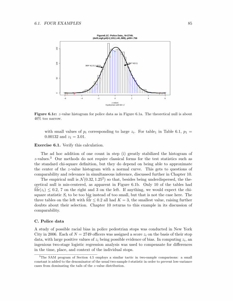
Figure 6.1c: z-value histogram for police data as in Figure 6.1a. The theoretical null is about40% too narrow.

with small values of pi corresponding to large zi. For table1 in Table 6.1, p1 =0.00132 and z1 = 3.01.

Exercise 6.1. Verify this calculation.

The ad hoc addition of one count in step (i) greatly stabilized the histogram ofz-values.3 Our methods do not require classical forms for the test statistics such asthe standard chi-square definition, but they do depend on being able to approximatethe center of the z-value histogram with a normal curve. This gets to questions ofcomparability and relevance in simultaneous inference, discussed further in Chapter 10.

The empirical null is N (0.32, 1.252) so that, besides being underdispersed, the the-oretical null is mis-centered, as apparent in Figure 6.1b. Only 10 of the tables hadf̂dr(zi) ≤ 0.2, 7 on the right and 3 on the left. If anything, we would expect the chi-square statistic Si to be too big instead of too small, but that is not the case here. Thethree tables on the left with f̂dr ≤ 0.2 all had K = 3, the smallest value, raising furtherdoubts about their selection. Chapter 10 returns to this example in its discussion ofcomparability.

C. Police data

A study of possible racial bias in police pedestrian stops was conducted in New YorkCity in 2006. Each of N = 2749 officers was assigned a score zi on the basis of their stopdata, with large positive values of zi being possible evidence of bias. In computing zi, aningenious two-stage logistic regression analysis was used to compensate for differencesin the time, place, and context of the individual stops.

3The SAM program of Section 4.5 employs a similar tactic in two-sample comparisons: a smallconstant is added to the denominator of the usual two-sample t-statistic in order to prevent low-variancecases from dominating the tails of the z-value distribution.


−4 −2 0 2 4

010

020

030

040

0

Figure6.1D: HIV data, N=7680,(del0,sig0,pi0)=(.116,.774,.949), pi00=1.20

128 genes with fdr<.2z values

.949*N(.116,.774^2)

N(0,1)

Figure 6.1d: z-value histogram for HIV data as in Figure 6.1a. Notice reduced scale on x-axis.In this case the theoretical null is too wide.

Let xij represent the vector of covariates for officer i, stop j. A greatly oversimplifiedversion of the logistic regression model actually used is

logit {Pr(yij = 1)} = βi + γ ′xij (6.4)

where yij indicates whether or not the stopped person was a member of a defined minor-ity group, βi is the “officer effect”, and γ is the vector of logistic regression coefficientfor the covariates. The z-score for officer i was

zi = β̂i

/se(β̂i

)(6.5)

where β̂i and se(β̂i) are the usual estimate and approximate standard error for βi.A standard analysis would rely on the theoretical null hypothesis zi ∼̇ N (0, 1).

However, the histogram of all N = 2749 zi values is much wider, the empirical null beingf̂0 ∼ N (0.10, 1.402). This resulted in 9 officers having f̂dr(zi) ≤ 0.20, only 4 of whomwere on the right (i.e., “racially biased”) side. The estimated non-null proportion wasπ̂1 = 0.011, only about 1/5 of which applied to the right side according to the smoothednon-null counts (5.41).

There is a lot at stake here. Relying on the theoretical N (0, 1) null gives π̂1 = 0.24,more than 20 times greater and yielding 122 officers having positive z-scores withf̂dr(zi) ≤ 0.20. The argument for empirical null analysis says we should judge theextreme z-scores by comparison with central variability of the histogram and not ac-cording to a theoretical standard. Section 6.4 provides practical arguments for doubtingthe theoretical standard.

D. HIV data

This was a small study in which n2 = 4 HIV-positive subjects were compared withn1 = 4 healthy controls using cDNA microarrays that measured expression levels for


mu and z −>

g(m

u) a

nd f(

z) −

>

−2 −1 0 1 2 3 4

050

100

150

200

250

^ ^1.5

f(z)

g(mu)

−2 0 2 4

0.0

0.2

0.4

0.6

0.8

1.0

z −>

Pro

b{N

ull |

z} a

nd fd

r(z)

*****

****

****

***************************

****

**************

*******************************************

Bayes

Emp null

Theo null

Figure 6.1e: Left panel : histogram shows N = 3000 draws from prior density g(µ) (6.6); curvef(z) is corresponding density of observations z ∼ N (µ, 1). Right panel : heavy curve is Bayesposterior probability Pr{µ ≤ 1.5|z}; it is well approximated by the empirical null estimate f̂dr(z)(6.9), light curve; fdr(z) based on the theoretical null f0 ∼ N (0, 1) is a poor match to the Bayescurve.

N = 7680 genes. Two-sample t-tests (on the logged expressions) yielded z-values zi asin (2.2)–(2.5) except now with 6 rather than 100 degrees of freedom.

Unlike all of our previous examples (including the prostate and DTI studies), herethe central histogram is less dispersed than a theoretical N (0, 1) null, with f̂0(z) ∼N (0.12, 0.772) and π̂0 = 0.949. (Underdispersion makes the theoretical null estimateequal the impossible value π̂00 = 1.20.) Using the theoretical null rather than theempirical null reduces the number of genes having f̂dr ≤ 0.2 from 128 to 20.

Figure 6.1e concerns an artificial example involving an overdispersed null distribu-tion, similar to the leukemia, chi-square, and police situations. Pairs (µi, zi) have beenindependently generated according to the Bayesian hierarchical model (2.47), µ ∼ g(·)and z|µ ∼ N (µ, 1); the prior density g(µ), represented as a histogram in the left panel,is bimodal,

g(µ) = 0.9 · ϕ0,0.5(µ) + 0.1 · ϕ2.5,0.5(µ) (6.6)

where ϕa,b represents the density of a N (a, b2) distribution. However, the mixturedensity f(z) =

∫g(µ)ϕ(z − µ)dµ is unimodal, reflecting the secondary mode of g(µ)

only by a heavy right tail.A large majority of the true effects µ generated from (6.6) will have small uninter-

esting values centered at, but not exactly equaling, zero. The interesting cases, thosewith large µ, will be centered around 2.5. Having observed z, we would like to pre-dict whether the unobserved µ is interesting or uninteresting. There is no sharp nullhypothesis here, but the shape of g(µ) suggests defining

Uninteresting : µ ≤ 1.5 and Interesting : µ > 1.5. (6.7)


The heavy curve in the right panel is the Bayes prediction rule for “uninteresting”,

Pr{µ ≤ 1.5|z}. (6.8)

This assumes that prior density g(µ) is known to the statistician. But what if it isn’t?The curve marked “Emp null” is the estimated local false discovery rate

f̂dr(z) = π̂0f̂0(z)/f̂(z) (6.9)

obtained using the central matching method of Section 6.2 which gave empirical nullestimates

π̂0 = 0.93 and f̂0(z) ∼ N (0.02, 1.142) (6.10)

based on N = 3000 observations zi. We see that it nicely matches the Bayes predictionrule, even though it did not require knowledge of g(µ) or of the cutoff point 1.5 in (6.7).

The point here is that empirical null false discovery rate methods can deal with“blurry” null hypotheses, in which the uninteresting cases are allowed to deviate some-what from a sharp theoretical null formulation. (Section 6.4 lists several reasons this canhappen.) The empirical null calculation absorbs the blur into the definition of “null”.Theoretical or permutation nulls fail in such situations, as shown by the beaded curvein the right panel.

6.2 Empirical Null Estimation

A null distribution is not something one estimates in classic hypothesis testing theory4:theoretical calculations provide the null, which the statistician must use for better orworse. Large-scale studies such as the four examples in Section 6.1 can cast severe doubton the adequacy of the theoretical null. Empirical nulls, illustrated in the figures, useeach study’s own data to estimate an appropriate null distribution. This sounds circularbut isn’t. We will see that a key assumption for empirically estimating the null is thatπ0, the proportion of null cases in (2.7), is large, say

π0 ≥ 0.90 (6.11)

as in (2.8), allowing the null distribution opportunity to show itself.The appropriate choice of null distribution is not a matter of local fdr versus tail area

Fdr: both are equally affected by an incorrect choice. Nor is it a matter of parametricversus nonparametric procedures. Replacing t-statistics with Wilcoxon test statistics(each scaled to have mean 0 and variance 1 under the usual null assumptions) givesempirical null f̂0(z) ∼̇ N (0.12, 1.722) for the leukemia data, almost the same as inFigure 6.1a.

The two-groups model (2.7) is unidentifiable: a portion of f1(z) can be redefined asbelonging to f0(z) with a corresponding increase in π0. The zero assumption (4.44),that the non-null density f1(z) is zero near z = 0, restores identifiability and allowsestimation of f0(z) and π0 from the central histogram counts.

4An exception arising in permutation test calculations is discussed in Section 6.5.

6.2. EMPIRICAL NULL ESTIMATION 89

Exercise 6.2. Suppose π0 = 0.95, f0 ∼ N (0, 1), and f1 is an equal mixture of N (2.5, 1)and N (−2.5, 1). If we redefine the situation to make (4.44) true in A0 = [−1, 1], whatare the new values of π0 and f0(z)?

Define

fπ0(z) = π0f0(z) (6.12)

so that

fdr(z) = fπ0(z)/f(z), (6.13)

(5.2). We assume that f0(z) is normal but not necessarily N (0, 1), say

f0(z) ∼ N(δ0, σ

20

). (6.14)

This yields

log (fπ0(z)) =[log(π0)− 1

2

{δ2

0

σ20

+ log(2πσ2

0

)}]+δ0

σ20

z − 12σ2

0

z2, (6.15)

a quadratic function of z.Central matching estimates f0(z) and π0 by assuming that log(f(z)) is quadratic

near z = 0 (and equal to fπ0(z)),

log (f(z)) .= β0 + β1z + β2z2, (6.16)

estimating (β0, β1, β2) from the histogram counts yk (5.12) around z = 0 and matchingcoefficients between (6.15) and (6.16): yielding σ2

0 = −1/(2β2) for instance. Note thata different picture of matching appears in Chapter 11.

Exercise 6.3. What are the expressions for δ0 and π0?

Figure 6.2 shows central matching applied to the HIV data of Section 6.1. Thequadratic approximation log f̂π0(z) = β̂0 + β̂1z+ β̂2z

2 was computed as the least squarefit to log f̂(z) over the central 50% of the z-values (with the calculation discretized asin Section 5.2) yielding (

δ̂0, σ̂0, π̂0

)= (0.12, 0.75, 0.93). (6.17)

These differ slightly from the values reported in Section 6.1 because those were calculatedusing the MLE method of Section 6.3.

The zero assumption (4.44) is unlikely to be literally true in actual applications.Nevertheless, central matching tends to produce nearly unbiased estimates of f0(z), atleast under conditions (2.47), (2.49):

µ ∼ g(·) and z|µ ∼ N (µ, 1),g(µ) = π0I0(µ) + π1g1(µ).

(6.18)


−3 −2 −1 0 1 2 3

23

45

6

Hiv data: central matching estimates: del0=.12, sig0=.75, pi0=.93

z value

log(

fhat

(z)

●

log fhat(z)

quadraticapproximation

Figure 6.2: Central matching estimation of f0(z) and π0 for the HIV data of Section 6.1,(6.15)–(6.16): (δ̂0, σ̂0, π̂0) = (0.12, 0.75, 0.93). Chapter 11 gives a different geometrical pictureof the matching process.

Here f0(z) = ϕ(z), the N (0, 1) density, but we are not assuming that the non-nulldensity

f1(z) =∫ ∞−∞

g1(µ)ϕ(z − µ) dµ (6.19)

satisfies the zero assumption. This introduces some bias into the central matchingassessment of δ0 and σ0 but, as it turns out, not very much as long as π1 = 1 − π0 issmall.

With π0 fixed, let (δg, σg) indicate the value of (δ0, σ0) obtained under model (6.18)by an idealized version of central matching based on f(z) =

∫∞−∞ g(µ)ϕ(z − µ)dµ,

δg = arg max {f(z)} and σg =[− d2

dz2log f(z)

]−12

δg

. (6.20)

Exercise 6.4. What values of β0, β1, β2 are implied by (6.20)? In what sense is (6.20)an idealized version of central matching?

We can ask how far (δg, σg) deviates from the actual parameters (δ0, σ0) = (0, 1) forg(µ) in (6.18). For a given choice of π0, let

δmax = max{|δg|} and σmax = max{σg}, (6.21)

the maxima being over the choice of g1 in (6.18). Table 6.2 shows the answers. Inparticular, for π0 ≥ 0.90 we always have

|δg| ≤ 0.07 and σg ≤ 1.04 (6.22)

so no matter how the non-null cases are distributed, the idealized central matchingestimates won’t be badly biased.

6.2. EMPIRICAL NULL ESTIMATION 91

Table 6.2: Worst case values δmax and σmax (6.21) as a function of π1 = 1− π0.

π1 = 1− π0 : .05 .10 .20 .30

σmax : 1.02 1.04 1.11 1.22δmax : .03 .07 .15 .27

0.0 0.1 0.2 0.3 0.4

0.0

0.5

1.0

1.5

pi1=1−pi0

Symm Normal

Symmetric

General

SIGmax

DELmax General

0.1

Figure 6.3: δmax and σmax (6.21) as a function of π1 = 1 − π0; symmetric restricts g1(µ) in(6.18) to be symmetric around µ = 0 and similarly symm normal.

Exercise 6.5. Show that σg ≥ 1 under model (6.18).

Figure 6.3 graphs δmax and σmax as a function of π1 = 1 − π0. In addition to thegeneral model (6.18), which provided the numbers in Table 6.2, σmax is also graphed forthe restricted version of (6.18) in which g1(µ) is required to be symmetric about µ = 0,and also the more restrictive version in which g1 is both symmetric and normal. Theworst-case values in Table 6.2 have g1(µ) supported on a single point. For example,σmax = 1.04 is achieved with g1(µ) supported at µ1 = 1.47.

The default option in locfdr is the MLE method, discussed in the next section, notcentral matching. Slight irregularities in the central histogram, as seen in Figure 6.1a,can derail central matching. The MLE method is more stable, but pays the price ofpossibly increased bias.

Here is a derivation of σmax for the symmetric case in Figure 6.3, the derivations forthe other cases being similar. For convenience we consider discrete distributions g(µ)in (6.18), putting probability π0 on µ = 0 and πj on pairs (−µj , µj), j = 1, 2, . . . , J , so


the mixture density equals

f(z) = π0ϕ(z) +J∑j=1

πj [ϕ(z − µj) + ϕ(z + µj)]/

2. (6.23)

Then we can take δj = 0 in (6.20) by symmetry (0 being the actual maximum if π0

exceeds 0.50). We consider π0 fixed in what follows.Defining c0 = π0/(1− π0), rj = πj/π0, and r+ =

∑J1 rj , we can express σg in (6.20)

as

σg = (1−Q)−12 where Q =

∑J1 rjµ

2je−µ2

j/2

c0r+ +∑J

1 rje−µ2

j/2. (6.24)

Actually, r+ = 1/c0 and c0r+ = 1, but the form in (6.24) allows unconstrained maxi-mization of Q (and of σg) as a function of r = (r1, r2, . . . , rJ), subject only to rj ≥ 0for j = 1, 2, . . . , J .

Exercise 6.6. Verify (6.24).

Differentiation gives

∂Q

∂rj=

1den

[µ2je−µ2

j/2 −Q ·(c0 + e−µ

2j/2)]

(6.25)

with den the denominator of Q in (6.24). At a maximizing point r we must have

∂Q(r)∂rj

≤ 0 with equality if rj > 0. (6.26)

Defining Rj = µ2j/(1 + c0e

µ2j/2), (6.25)–(6.26) give

Q(r) ≥ Rj with equality if rj > 0. (6.27)

At the point where Q(r) is maximized, rj and πj can only be nonzero if j maximizesRj .

All of this shows that we need only consider J = 1 in (6.23). (In case of ties in(6.27) we can arbitrarily choose one of the maximizing j values.) The maximized valueof σg is then σmax = (1−Rmax)−1/2 from (6.24) and (6.27), where

Rmax = maxµ1

{µ2

1

/(1 + c0e

µ21/2)}

. (6.28)

The maximizing argument µ1 ranges from 1.43 for π0 = 0.95 to 1.51 for π0 = 0.70. Thisis considerably less than choices such as µ1 = 2.5, necessary to give small false discoveryrates, at which the values in Figure 6.3 will be conservative upper bounds.

6.3. THE MLE METHOD FOR EMPIRICAL NULL ESTIMATION 93

6.3 The MLE Method for Empirical Null Estimation

The MLE method takes a more straightforward approach to empirical null estimation:starting with the zero assumption (4.44), we obtain normal theory maximum likelihoodestimators (δ̂0, σ̂0, π̂0) based on the zi values in A0. These tend to be less variable thancentral matching estimates, though more prone to bias.

Given the full set of z-values z = (z1, z2, . . . , zN ), let N0 be the number of zi in A0

and I0 their indices,I0 = {i : zi ∈ A0} and N0 = #I0 (6.29)

and define z0 as the corresponding collection of z-values,

z0 = {zi, i ∈ I0} . (6.30)

Also, let ϕδ0,σ0(z) be the N (δ0, σ20) density function

ϕδ0,σ0(z) =1√

2πσ20

exp

{−1

2

(z − δ0

σ0

)2}

(6.31)

andH0(δ0, σ0) ≡

∫A0

ϕδ0,σ0(z) dz, (6.32)

this being the probability that a N (δ0, σ20) variate falls in A0.

We suppose that the N zi values independently follow the two-groups model (2.7)with f0 ∼ N (δ0, σ

20) and f1(z) = 0 for z ∈ A0. (In terms of Figure 2.3, A0 = Z, N0 =

N0(A0), and N1(A0) = 0.) Then z0 has density and likelihood function

fδ0,σ0,π0(z0) =[(

N

N0

)θN0(1− θ)N−N0

]∏I0

ϕδ0,σ0(zi)H0(δ0, σ0)

(6.33)

whenθ = π0H0(δ0, σ0) = Pr {zi ∈ A0} . (6.34)

Notice that z0 provides N0 = #z0, distributed as Bi(N, θ), while N is a known constant.

Exercise 6.7. Verify (6.33).

Exponential family calculations, described at the end of the section, provide theMLE estimates (δ̂0, σ̂0, π̂0). These are usually not overly sensitive to the choice of A0,which can be made large in order to minimize estimation error. Program locfdr centersA0 at the median of z1, z2, . . . , zN , with half-width about 2 times a preliminary estimateof σ0 based on interquartile range. (The multiple is less than 2 if N is very large.)

Table 6.3 reports on the results of a small Monte Carlo experiment: measurementszi were obtained from model (2.7) with π0 = 0.95, f0 ∼ N (0, 1), f1 ∼ N (2.5, 1) andN = 3000. The zi values were not independent, having root mean square correlationα = 0.10; see Chapter 8. One hundred simulations gave means and standard deviationsfor (δ̂0, σ̂0, π̂0) obtained by central matching and by the MLE method.


Table 6.3: MLE and central matching estimates (δ̂0, σ̂0, π̂0) from 100 simulations with π0 =0.95, f0 ∼ N (0, 1), f1 ∼ N (2.5, 1), N = 3000, and root mean square correlation 0.10 betweenthe z-values. Also shown is correlation between MLE and CM estimates.

δ̂0 σ̂0 π̂0

MLE CM MLE CM MLE CM

mean : −.093 −.129 1.004 .984 .975 .963stdev : .016 .051 .067 .098 .008 .039

corr : .76 .89 .68

The MLE method yielded smaller standard deviations for all three estimates. It wassomewhat more biased, especially for π0. Note that each 3000-vector z had its meansubtracted before the application of locfdr so the true null mean δ0 was −0.125 not 0.

Besides being computationally more stable than central matching of Figure 6.2, theMLE method benefits from using more of the data for estimation, about 94% of thecentral z-values in our simulation, compared to 50% for central matching. The lattercannot be much increased without some danger of eccentric results. The upward biasof the MLE π̂0 estimate has little effect on f̂dr(z) or F̂dr(z) but it can produce overlyconservative estimates of power (Section 5.4). Taking a chance on more parametricmethods (see Notes) may be necessary here.

Straightforward computations produce maximum likelihood estimates (δ̂0, σ̂0, π̂0) in(6.33); fδ0,σ0,π0(z0) is the product of two exponential families5 which can be solvedseparately (the two bracketed terms). The binomial term gives

θ̂ = N0/N (6.35)

while δ̂0 and σ̂0 are the MLEs from a truncated normal family, obtained by familiariterative calculations, finally yielding

π̂0 = θ̂/H0

(δ̂0, σ̂0

)(6.36)

from (6.34). The log of (6.33) is concave in (δ0, σ0, π0) guaranteeing that the MLEsolutions are unique.

Exercise 6.8. Show that (6.33) represents a three-parameter exponential family. Thatis,

log fδ0,σ0,π0(z0) = η1Y1 + η2Y2 + η3Y3 − ψ(η1, η2, η3) + c(z0) (6.37)

where (η1, η2, η3) are functions of (δ0, σ0, π0) and (Y1, Y2, Y3) are functions of z0. Whatare (η1, η2, η3) and (Y1, Y2, Y3)?

5Appendix A gives a brief review of exponential families.

6.4. WHY THE THEORETICAL NULL MAY FAIL 95

6.4 Why the Theoretical Null May Fail

The four examples in Figure 6.1 strongly suggest failure of the theoretical null distri-bution f0(z) ∼ N (0, 1). This is somewhat shocking! Theoretical null derivations likethat for Student’s t-distribution are gems of the statistical literature, as well as pillarsof applied practice. Once alerted however, it isn’t difficult to imagine causes of failurefor the theoretical null. The difference in large-scale testing is only that we can detectand correct such failures.

Making use of either central matching or the MLE method, false discovery rateestimates (5.5) and (5.6) now become

f̂dr(z) = π̂0f̂0(z)/f̂(z) and F̂dr(z) = π̂0F̂0(z)

/F̂ (z) (6.38)

with F̂0(z) the left or right cdf of f̂0(z) as desired. (6.38) is not a universal improve-ment over (5.5)–(5.6); estimating the null distribution f0(z) substantially adds to thevariability of false discovery rate estimates, as documented in Chapter 7. But using thetheoretical null when it is wrong is a recipe for false inference. What follows is a list ofpractical reasons why the theoretical null might go astray.

I. Failed mathematical assumptions Textbook null hypothesis derivations usually be-gin from an idealized mathematical framework, e.g., independent and identically dis-tributed (i.i.d.) normal components for a two-sample t-statistic. Deviations from theideal can be easy to spot in large-scale data sets. For example, the logged expressionlevels xij for the HIV data have longer-than-normal tails. (Although, by itself, that isnot enough to induce the underdispersion seen in the z-value histogram of Figure 6.1d:repeating the HIV computation for a 7680×8 matrix whose components were randomlyselected from the actual matrix gave an almost perfectly N (0, 1) z-value histogram.)

II. Correlation across sampling units Student’s theoretical null distribution for a two-sample t-statistic (2.2) assumes independence across the n sampling units: for instance,across the 72 patient scores for any one gene in the leukemia study. Chapter 8 shows howsuch independence assumptions can fail in practice. In large-scale studies, even minorexperimental defects can manifest themselves as correlation across sampling units. Theexpression levels xij for the prostate study of Section 2.1 will be seen to have driftedslightly as the experiment went on (i.e., as j increased), some genes drifting up andothers down, inducing minor correlations across microarrays. Other data sets will showmore significant correlations, big enough to seriously distort the z-value histogram.

III. Correlation across cases It was argued in Section 4.4 that independence amongthe z-values is not required for valid false discovery rate inference. The hitch is thatthis is only true if we are using the correct null distribution f0(z). Section 8.3 discussesthe following disconcerting fact: even if the theoretical null distribution zi ∼ N (0, 1) isvalid for all null cases, correlation among the zi can make N (0, 1) a misleading choicein likely realizations of z = (z1, z2, . . . , zN ).

Figure 6.4 provides an example. A simulation study was run with N = 6000 z-values; 5700 were null cases having zi ∼ N (0, 1), with root mean square correlation0.1 among the 5700 · 5699/2 pairs. The 300 non-null cases followed an exact N (2.5, 1)


●

●

●

●

●

●

●●

●●●

●

●

●

●

●

●

●

●

●

●

●

●

●

●

●

●

●

●

●

●

●

●

●

●

●

●

●

●

●

●

●

●

●

●

●

● ●

●

●

●

●●

●

●

●

●

●

●

●

●

●

●

● ●

●

●

●

●

●

●

●

●

●

●

●

●

●

●

●

●

●

●

●

●

●

●

●

●

●

●

●●

●

●●

●

●

●

●

0.05 0.10 0.15 0.20 0.25 0.30 0.35

0.1

0.2

0.3

0.4

0.5

0.6

Fdp

Fdr

hat

●●

●●●

●

●●●

●

●●

●

●●

●

●

●

●

●

●

●

●

●

●

●

●●

●

●● ●●

●

●

●●

●

●●

●

●

●

●

●

●● ● ●

●

●

●

●

●

●

●

●

●

●

●

●●

● ●

●

●

●

●●

●

●

●

●●

●

●

●●

●

●

●

●

●

●●

●

●●

●●

●

●●

●

●●

●

●

●

●

circles=Fdrhatnull

Figure 6.4: Simulation experiment comparing empirical null and theoretical null estimates ofFdr(2.5), plotted against actual False discovery proportion Fdp(2.5), as described in text. Thetheoretical null estimates (open circles) decrease as Fdp increases.

distribution, that is,

zi = 2.5 + Φ−1

(i− 0.5

300

)for i = 1, 2, . . . , 300. (6.39)

Three quantities were calculated for each of 100 simulations,

Fdp(2.5) =#{null zi ≥ 2.5}

#{zi ≥ 2.5}, (6.40)

the actual false discovery proportion (2.28) for Z = [2.5,∞), and both F̂drtheo(2.5) andF̂dremp(2.5), the theoretical and empirical null Fdr estimates (5.6) and (6.38).

The two Fdr estimates are plotted versus Fdp in Figure 6.4. Correlation betweenthe null cases makes Fdp(2.5) highly variable. F̂dremp(2.5) follows Fdp(2.5), somewhatnoisily, but F̂drtheo(2.5) moves in the wrong direction, slowly decreasing as Fdp in-creases. F̂dremp is much more variable than F̂drtheo but nevertheless more accurate asan estimate of Fdp, with mean |F̂dremp(2.5) − Fdp(2.5)| = 0.065 compared to mean|F̂drtheo(2.5)− Fdp(2.5)| = 0.098. Even though the theoretical N (0, 1) null is uncondi-tionally correct here, it is unsatisfactory conditionally.

Exercise 6.9. Explain why F̂drtheo(2.5) is a decreasing function of Fdp(2.5).

IV. Unobserved covariates Except for the chi-square data, all of our examples areobservational studies. The 72 leukemia patients were observed, not assigned, to be inthe AML or ALL class. Unobserved covariates such as age, gender, concomitant health

6.4. WHY THE THEORETICAL NULL MAY FAIL 97

conditions, processing variables6, etc., may affect the AML/ALL comparison. If thecovariates were available we could use linear model techniques to account for them, butif not they tend to broaden the effective null distribution f0, as discussed next.

Suppose we have a microarray experiment comparing n/2 Class A subjects with n/2Class B subjects, for N genes. The null genes are assumed to have expression levels

xij = uij +Ij2βi

{uij ∼ N (0, 1)βi ∼ N (0, σ2

β)(6.41)

with ui1, ui2, . . . , uin, βi mutually independent, and

Ij =

{−1 j = 1, 2, . . . , n/21 j = n/2 + 1, . . . , n.

(6.42)

Here the βi values are small disturbances caused by unequal effects of unobserved co-variates on the two classes. (The βi may be correlated across genes.)

It is easy to show that the two-sample t-statistic ti (2.2) comparing Class A withClass B follows a dilated t-distribution with n− 2 degrees of freedom,

ti ∼(

1 +n

4σ2β

)12 · tn−2 (6.43)

for the null cases. In other words, the null density is (1+nσ2β/4)1/2 times more dispersed

than the usual theoretical null.

Exercise 6.10. (a) Verify (6.43). (b) Suppose that all the genes are null and thatσβ = 2/

√n. Show that for large N the local fdr, with π0 = 1, will be about

fdr(ti).=√

2fn−2(ti)/fn−2

(ti

/√2)

(6.44)

when f0 is taken to be the usual theoretical null fn−2(t), a Student t-density with n− 2degrees of freedom. (c) For n = 20, what is the probability that fdr(ti) ≤ 0.20 under(6.44)?

The empirical null fdr estimate π̂0f̂0(z)/f̂(z) scales “correctly” using either centralmatching or the MLE method: if each zi is multiplied by the same positive constant c,the value of f̂dr stays the same for all cases. Another way to say this is that our interestin an outlying zi is judged relative to the width of the histogram’s center, rather thanrelative to the theoretical N (0, 1) width.

Unobserved covariates are ubiquitous in large-scale studies and are perhaps the mostcommon source of trouble for the theoretical null, a likely culprit for the kind of grossoverdispersion seen in Figure 6.1a. Reason III above, correlation across cases, producessmaller effects, but is capable of causing the underdispersion seen in Figure 6.1d as wellas overdispersion (Chapter 7). Microarray studies are particularly prone to correlation

6For example, different areas on a microarray chip are read separately, by devices that may becalibrated differently.


effects, as the examples of Chapter 8 will show. Reason II, correlation across the sup-posedly independent sampling units, is surprisingly prevalent as a possible source ofoverdispersion (Chapter 8). Failed mathematical assumptions, Reason I, is the only oneof the four failure causes that is easily cured by permutation calculations, as discussedin the next section.

Our list of causes is by no means complete. Filtration, the data-based preselectionof a subset of promising-looking cases for final analysis, can distort both the null andnon-null distributions. In a microarray context the investigator might first select onlythose genes having above-average standard deviations, on the grounds that this hints atdifferential response across the various experimental conditions. Filtration is a danger-ous tactic. Among other dangers, it reduces, in a biased manner, information availablefor evaluating the appropriate null distribution.

6.5 Permutation Null Distributions

Permutation techniques for assessing a null distribution lie somewhere between thetheoretical and empirical methods, but closer to the former than the latter. They areeasiest to describe in two-sample situations like the prostate, leukemia, and HIV studies.We have an N × n data matrix X with the first n1 columns representing Treatment 1and the last n2 columns Treatment 2. These have produced an N -vector z of z-values,perhaps as in (2.2)–(2.5).

In order to compute the permutation null distribution, we randomly permute thecolumns of X as in (3.39) and recalculate the vector of z-values. Repeating the processB times gives vectors z∗1, z∗2, . . . ,z∗B, with

Z∗ =(z∗1, z∗2, . . . ,z∗B

)(6.45)

representing the full N × B matrix of permuted values. The usual permutation null isthen

f̂perm0 = the empirical distribution of all N ·B values z∗bi . (6.46)

(Less commonly, we might calculate a separate permutation null for each case i fromthe B values in the ith row of Z∗. This requires B to be very large in order to assessthe extreme tail probabilities necessary in large-scale testing, whereas B = 10 or 20 isoften sufficient for (6.46).)

Figure 6.5 shows QQ plots7 of f̂perm0 for the leukemia and HIV studies (z-values as

in (2.2)–(2.5)), in both cases based on B = 20 permutations. The leukemia plot showsf̂perm

0 nearly N (0, 1) while f̂perm0 (z) for the HIV data is roughly N (0, 0.962) near z = 0,

but with heavier-than-normal tails.Permutation methods offer a simple and attractive way to deal with mathematically

complicated hypothesis testing situations. They are not however a remedy for thetheoretical null failures seen in Figure 6.1. There are several points to consider:

7A QQ plot of observations x1, x2, . . . , xm plots the ith ordered value x(i) versus the correspondingnormal quantile Φ−1[(i − 0.5)/m]. If the x values come from a N (a, b2) distribution, the plot willapproximate a straight line with intercept a and slope b.

6.5. PERMUTATION NULL DISTRIBUTIONS 99

−4 −2 0 2 4

−4

−2

02

4

Leukemia data

inter= −0.001 slope= 1.015

−4 −2 0 2 4

−4

−2

02

46

HIV data

inter= −0.008 slope= 0.956

Figure 6.5: QQ plots of permutation null distributions for the leukemia and HIV studies,B = 20 permutations each. Dotted lines are least squares fits to central 80% of the plot, withintercepts and slopes as indicated; f̂perm

0 ∼̇ N (0, 1) for leukemia study but has heavier tails forHIV study.

• Of the four potential causes of failure raised in Section 6.4, permutation meth-ods deal most effectively with Reason I, failed mathematical assumptions. Thepermutation process enforces an i.i.d. structure, so that f̂perm

0 is relevant only inthat context. (The second i, “identical”, may not be realistic, but this usuallydoesn’t seem to cause major problems.) Non-standard statistical definitions —for example, adding a constant to the usual t-statistic denominator, as in SAM —are automatically incorporated into the permutation calculations.

• Permutation methods are no help with Reason II, correlation across samplingunits, since the sampling process effectively enforces independence.8

• They are also of no help with Reason IV, unobserved covariates. The data vector(xi1, xi2, . . . , xin) in (6.41) has βi/2 subtracted from the first n/2 observationsand added to the last n/2. But as far as permutation samples are concerned,the ±βi/2 disturbances are randomly distributed across the n observations. Thepermutation distribution of the two-sample t-statistic is nearly tn−2 under model(6.41) no matter how large βi may be, rather than equaling the dilated distribution(6.43).

• A virtue of permutation methods is that they preserve correlation between cases,e.g., between genes (since the columns ofX are permuted intact). We can estimatethe correlation between any pair of z-values from the correlation between the rowsof Z∗ (6.45), as was done in Section 3.4 and will be seen again in Chapter 8.

Nevertheless, permutation methods are of no direct assistance with Reason III, theeffects of between-case correlations on the proper choice of f0. For any given row

8It actually enforces a small negative correlation: if x∗1 and x∗2 are any two draws in a permutationsample, then their correlation is −1/(n− 1) with respect to the permutation process, regardless of thecorrelations in the original sample x1, x2, . . . , xn.


i of Z∗, the values z∗bi do not depend on between-case correlations, and neitherdoes f̂perm

0 . Both the leukemia and HIV examples display considerable case-wisecorrelation (see Chapter 8) but still have f̂perm

0 close to the theoretical null andfar from the empirical null.

• In fact, f̂perm0 will usually approximate a N (0, 1) distribution for (2.5), the z-

score version of the t-statistic. Fisher’s introduction of permutation argumentswas intended to justify Student’s distribution in just this way. A considerablebody of theory in the 1950s showed f̂perm

0 converging quickly to N (0, 1) as n grewlarge. The results in Figure 6.5 are typical, showing almost perfect convergencein the leukemia example, n = 72.

• Permutation and empirical methods can be combined by letting the permutationnull replace N (0, 1) in the empirical algorithm. That is, we perform the empiricalnull calculations on Φ−1(Fperm(zi)) rather than on the original z-values, withFperm the permutation cdf. Doing so made no difference to the leukemia data butconsiderably increased f̂dr for the HIV data, reducing the number of cases withf̂dr ≤ 0.20 from 128 to 42, now all on the left side.

• Permutation methods are not restricted to two-sample problems. They depend onsymmetries of the null hypothesis situation, which may or may not exist. Theywould be difficult to find, perhaps impossible, for the chi-square and police ex-amples of Figure 6.1. Bootstrap methods are more flexible but have their ownproblems in large-scale situations; see Section 7.5.

Notes

The leukemia data was the motivating example in Golub et al. (1999), an early ex-ploration of advanced statistical approaches to microarray experiments. Ridgeway andMacDonald (2009) discuss the police data, providing a much more extensive analysisthan the one here. Van’t Wout et al. (2003) originated the HIV data, which was usedas a main example in Gottardo et al. (2006) as well as Efron (2007b). The chi-squaredata is part of an ongoing unpublished experiment.

Empirical null methods were introduced in Efron (2004), along with the centralmatching algorithm. Efron (2007b) suggested the MLE method. Why the theoreticalnull might fail is discussed in Efron (2008a). Jin and Cai (2007, 2009) present a char-acteristic function approach to estimating the empirical null, while a more parametricnormal mixture method is analyzed in Muralidharan (2009a).

The 1935 edition of Fisher’s The Design of Experiments introduced permutationmethods as a justification of Student’s t-test. A great deal of subsequent analysis bymany authors, including Pitman (1937) and Hoeffding (1952), supported Fisher’s con-tention that permutation methods usually agree closely with Student’s distribution.

theoretical, permutation and empirical null...

Documents