theoretical physics ii - github pagesa operator kung fu 117 b bibliography 121. introduction the...
TRANSCRIPT

A U S T E N L A M A C R A F T
T H E O R E T I C A L P H Y S I C S I I
T O P I C S I N Q U A N T U M T H E O R Y


Contents
1 Quantum Dynamics 7
2 Introduction to path integrals 23
3 Scattering theory 35
4 Density matrices 57
5 Second quantization 69
6 Introduction to Lie groups 91
7 Relativistic quantum mechanics 107
A Operator Kung Fu 117
B Bibliography 121


Introduction
The development of quantum theory during the 20th century led to the in-troduction of completely new concepts to physics. At the same time, physi-cists were forced – sometimes unwillingly – to adopt myriad new techniquesand mathematical ideas. In this course, we’ll survey some of these moreadvanced topics.
This course is recommended only for students who have achieved astrong performance in Mathematics as well as Physics in Part IB, or anequivalent qualification.
Outline of lectures
Topics in italics are non-examinable.
1. Quantum Dynamics [3 lectures]
Schrödinger, Heisenberg, interaction picture. The evolution operator andtime ordering. Driven oscillator. Coherent states. A spin- 1
2 in a field. Theadiabatic approximation. Landau-Zehner transitions. Berry’s phase.
2. Introduction to path integrals [1 lecture]
The propagator and the Green’s function: free particle and harmonicoscillator. The method of stationary phase and the semiclassical limit.
3. Scattering Theory [3 lectures]
Scattering in one dimension. Scattering amplitude and cross section.Optical theorem. Lippmann-Schwinger equation. Born series. Partialwave analysis. Bound states.
4. Density Matrices [2 lectures]
Density matrix and its properties. Applications in statistical mechanics.Density operator for subsystems and entanglement. Quantum damping.
5. Identical Particles in Quantum Mechanics [4 lectures]
Second quantisation for bosons and fermions. Single-particle densitymatrix and density-density correlation function. Bose-Hubbard model.Bogoliubov transformation. Interference of condensates.
6. Lie Groups [2 lectures]
Symmetries are groups. Lie algebra of generators. Rotations as Lie group.Representations of SO(3), SU(2), Lorentz group SO(1, 3) and SL(2, C).
7. Relativistic Quantum Physics [1 lecture]
Klein-Gordon equation. Antiparticles. Spinors and the Dirac equation.Relativistic covariance.

6 austen lamacraft
Books
A few good books at about the right level:
• JJ Sakurai, Modern Quantum Mechanics, 2nd edition, Addison-Wesley, 1994.
• F Schwabl, Quantum Mechanics, 4th edition, Springer 2007, and F Schwabl,Advanced Quantum Mechanics, 4th edition, Springer 2008.
• R Shankar Principles of Quantum Mechanics, 2nd edition, Springer 1994.
• G Baym, Lectures on Quantum Mechanics, W. A. Benjamin, 1969.
For more problems that you can shake a stick at, see the recently pub-lished Exploring Quantum Mechanics (CUP, 2013) by Galitski et al.. Rememberthat doing problems is the only way to cement your understanding of newconcepts!
For mathematical background I’d heartily recommend Mike Stone andPaul Goldbart’s Mathematics for Physicists: A guided tour for graduate students(CUP, 2009). This contains a lot of advanced material as well as much ofwhat you covered in 1B Mathematics.
A great resource for just about anything you may need to know about anyof the functions we meet is the NIST Digital Library of Mathematical Functionsat http://dlmf.nist.gov.
Structure of these lectures
You will find problems embedded in the text. Most of these are relativelyshort, and often involve checking expressions, or working through omittedsteps. They are therefore a vital part of the development. It’s probably bestto work through these immediately after (or during!) the lectures, and makea note of any points you don’t understand for the examples classes.
TANGENT Occasionally, you will see boxes of indented text like this. They in-
dicate background material that is not on the syllabus, but which you may find
interesting. You definitely don’t need to know anything that appears in one of
these comments (except this one). Some of these contain problems. Again, they are
just for added interest. The same applies to the Appendices to Chapter 3.
You are strongly encouraged, however, to immediately work through theproblems in Appendix A to improve your facility with the manipulation ofoperators. If you find this process excruciatingly painful, this may not be thecourse for you!
This course naturally builds on the Advanced Quantum Physics coursefrom Michaelmas, so I’ll sometimes refer back to these lectures with theabbreviation AQP.

1Quantum Dynamics
In this first chapter we’re going to introduce some general ideas of quantumdynamics, using the two simplest quantum systems: the harmonic oscillatorand a single spin-1/2.
1.1 The Quantum Harmonic Oscillator
There’s an old crack from the late quantum field theorist Sidney Coleman tothe effect that
The career of a young theoretical physicist consists of treating the harmonicoscillator in ever-increasing levels of abstraction.
There’s a large kernel of truth in this, for the simple reason that many sys-tems in physics vibrate, from bridges to quantum fields, and within a certainapproximation that vibration can be treated as harmonic. In this section weare going to remind ourselves about some features of quantum dynamics us-ing this model as our basic example, as it allows most results to be expressedanalytically. Along the way I’ll try and point out which features generalise tomore complicated systems (and which don’t!).
Time independent case
The Hamiltonian is
H =p2
2m+
12
mω2x2, (1.1)
where the position and momentum operators satisfy
[x, p] = ih.
The state of the oscillator |ψ〉 evolves in time according to the (time depen-dent) Schrödinger equation
ih∂
∂t|ψ〉 = H |ψ〉 . (1.2)
This is a first order differential equation, and so the evolution is fixed oncethe initial state |ψ(0)〉 is specified. We can write the solution as
|ψ(t)〉 = exp (−iHt/h) |ψ(0)〉 ≡ U(t) |ψ(0)〉 . (1.3)
The operator U(t) = e−iHt/h is called the evolution operator, as it evolves thestate |ψ(0)〉 forward in time.

8 austen lamacraft
Functions of operators can be thought of as defined by their power seriesexpansions, in this case
U(t) = 1− iHth− 1
2
(Hth
)2+ · · · . (1.4)
Alternatively, if an operator has a complete orthonormal eigenbasis |n〉 (asquantum observables do, being Hermitian operators), we can write anysuch function in terms of this basis and the corresponding function of theeigenvalues En
U(t) = ∑n
e−iEnt/h |n〉 〈n| . (1.5)
This latter point of view then focuses attention on the eigenstates |n〉. Tofind these there are at least two approaches
1. (Brute force) Take the position representation p = −ih ddx and study the
time independent Schrödinger equation in this representation
− h2
2md2ψn
dx2 +12
mω2x2ψn = Enψn (1.6)
where 〈x|n〉 = ψn(x). The result is that the eigenfunctions have the form
ψn(x) =1√2nn!
(mω
πh
)1/4e−mωx2/2h Hn
(√mω
hx)
(1.7)
with eigenvalues En = hω(n + 1/2), where Hn(z) are the Hermite polyno-mials
2. (More sophisticated) Define the hermitian conjugate pair
a =
√mω
2h
(x + i
pmω
)a† =
√mω
2h
(x− i
pmω
),
(1.8)
which satisfy[a, a†] = 1. (1.9)
The Hamiltonian is expressed as
H =hω
2
[a†a + aa†
]= hω(N + 1/2) (1.10)
where N ≡ a†a. The commutation relation Eq. (1.9) implies
[N, a] = −a [N, a†] = +a†, (1.11)
which in turn tells us that acting with a† (a) on an eigenstate |n〉of Nwith eigenvalue n gives another eigenstate with eigenvalue increased(decreased) by 1.
Alternatively, we can try and find U(t) indirectly, from the effect it hason operators. Recall that in the Heisenberg picture operators acquire a timedependence
O(t) = U†(t)OU(t), (1.12)
equivalent to the Heisenberg equation of motion
dO(t)dt
=ih[H,O(t)]. (1.13)

theoretical physics ii 9
Let’s see what this means for the Harmonic oscillator. Evidently H =
U†(t)HU(t), so
H = U†(t)HU(t) =p(t)2
2m+
12
mω2x(t)2. (1.14)
We have
dx(t)dt
=ih[H, x(t)] =
p(t)m
dp(t)dt
=ih[H, p(t)] = −mω2x(t)
(1.15)
You may recognize these equations as identical to Hamilton’s equations for theSHO
dxdt
=∂H∂p
=pm
dpdt
= −∂H∂x
= −mω2x(1.16)
Problem 1.1
Convince yourself that the same correspondence holds for the moregeneral Hamiltonian
H = T(p) + V(x) (1.17)
The general solution is
x(t) = cos(ωt)x(0) + sin(ωt)p(0)mω
p(t) = cos(ωt)p(0)−mω sin(ωt)x(0),(1.18)
and corresponds to a point tracing out an ellipical trajectory centred at theorigin in the x− p plane (phase space). From this point of view the operatorsa, a† in Eq. (1.8) can be seen as complex amplitudes whose phase changeslinearly in time
a(t) = e−iωta(0), a†(t) = e+iωta†(0). (1.19)
Problem 1.2
Verify that Eq. (1.19) follows directly from Eq. (1.1) and the commuta-tion relation Eq. (1.9).
Time dependent force
Mostly we don’t leave quantum systems to get on with their own time evo-lution, but disturb them in some way. For example, an atom may experiencean external radiation field. The prototype for this situation is the SHO sub-ject to a time dependent force Recall that in the Heisenberg picture
the Hamiltonian remained time in-dependent. Now it has intrinsic timedependenceH(t) =
p2
2m+
12
mω2x2 − F(t)x. (1.20)

10 austen lamacraft
How does such a system evolve? The important thing to realize is that thesolution of the Schrödinger equation
ih∂
∂t|ψ〉 = H(t) |ψ〉 . (1.21)
is notU(t) 6= exp (−iH(t)t/h) . (1.22)
Let’s consider the situation described by
F(t) =
F1 0 ≤ t < t1
F2 t1 ≤ t < t2. (1.23)
The evolution operator is
U(t) =
U1(t) 0 ≤ t < t1
U2(t− t1)U1(t1) t1 ≤ t < t2(1.24)
where Ui(t) = e−iHit/h and Hi =p2
2m + 12 mω2x2− Fix. It’s important to realize
that H1 and H2 don’t commute with each other
[H1, H2] = −ihpm(F1 − F2), (1.25)
thus U1 and U2 don’t commute and the product of U1 and U2 in Eq. (1.24) isnot easily written in terms of a single exponential.
The evolution operator corresponding to a general force F(t) can be un-derstood by splitting the evolution up into many small stages
U(t) = lim∆t→0
e−iH(t−∆t)∆t/he−iH(t−2∆t)∆t/h · · · e−iH(∆t)∆t/he−iH(0)∆t/h.
= lim∆t→0
(1− iH(t− ∆t)∆t
h
)(1− iH(t− 2∆t)∆t
h
)· · ·(
1− iH(0)∆th
)= 1− i
h
∫ t
0dt1 H(t1)−
1h2
∫ t
0dt2
∫ t2
0dt1 H(t2)H(t1) + . . . .
(1.26)
Note that the time arguments of H(t) are increasing from right to left. Thefinal expression for U(t) can be written in a dangerously compact fashion byusing the notation
T [H(t1)H(t2)] =
H(t1)H(t2) t1 ≥ t2
H(t2)H(t1) t2 > t1, (1.27)
and so on. The operation denoted by T is usually called time ordering. Wehave
U(t) = 1− ih
∫ t
0dt1 H(t1)−
12h2
∫ t
0dt2
∫ t
0dt1 T [H(t1)H(t2)] + . . . . (1.28)
Allowing the integrals to range over 0 < ti < t instead of ordering themnecessitates the introduction of a factor 1
n! at the nth order. This allows us towrite
U(t) = T exp(− i
h
∫ t
0dt′ H(t′)
)(1.29)

theoretical physics ii 11
This expression should be handled with extreme care! It evidently reduces toe−iHt/h in the case of a time-independent Hamiltonian. In the general case, itis only really useful in the form of the expansion Eq. (1.28).
To make progress in the case of the driven oscillator, it’s useful to onceagain consider the Heisenberg equations of motion
dx(t)dt
=ih[H, x(t)] =
p(t)m
dp(t)dt
=ih[H, p(t)] = −mω2x(t) + F(t).
(1.30)
In terms of a and a†
H(t) =hω
2
(a†a + aa†
)− F(t)
√h
2mω(a + a†), (1.31)
and we have
dadt
= −iωa + iF(t)
√1
2mhω. (1.32)
If we define a(t) = eiωta(t), we get
dadt
= +iF(t)eiωt√
2mhω, (1.33)
with general solution
a(t) = a(0) +i√
2mhω
∫ t
0F(t′)eiωt′dt′, (1.34)
and similarly
a†(t) = a†(0)− i√2mhω
∫ t
0F(t′)e−iωt′dt′. (1.35)
Problem 1.3
Satisfy yourself that this corresponds to the classical solution of a forcedoscillator.
What can we do with this solution? Suppose we start from the ground state,which satisfies
a |0〉 = 0. (1.36)
Since a(t) = U†(t)aU(t) we have aU(t) = U(t)a(t) and thus
aU(t) |0〉 = i√2mhω
∫ t
0F(t′)eiω(t′−t)dt′U(t) |0〉 , (1.37)
we have that U(t) |0〉 is an eigenstate of a(0) = a with eigenvalue
i√2mhω
∫ t
0F(t′)eiω(t′−t)dt′, (1.38)
in other words, it is a coherent state. Recall from AQP that a coherent state |α〉is defined as an eigenstate of a with eigenvalue α (generally complex, as a isnot Hermitian)
a |α〉 = α |α〉 . (1.39)
The explicit form of a normalized coherent state is
|α〉 = e−|α|2/2eαa† |0〉 , (1.40)
where both the property Eq. (1.39) and the normalization follow from thefundamental commutator [a, a†] = 1.

12 austen lamacraft
Problem 1.4
Prove this.
Note that the ground state |0〉 is a coherent state with α = 0.
Problem 1.5
Show that if we start in a coherent state |α〉, then after time t we are inthe state
U(t) |α〉 = eiφ(t) |α′〉 (1.41)
where
α′ = α +i√
2mhω
∫ t
0F(t′)eiωt′dt′. (1.42)
Find the form of the phase φ(t).
Problem 1.6
Verify that the result Eq. (1.38) is consistent with first order time de-pendent perturbation theory for the amplitude to transition to the firstexcited state.
1.2 A Spin in a Field
The simplest quantum system we can write down consists of just two states.Two state systems abound in physics.Or rather, many physical situations canbe approximated by considering onlytwo states. Some important examplesare the spin states of the electron, apair of atomic states coupled by exter-nal radiation, and the two equivalentpositions of the Nitrogen atom in thetrigonal pyramid structure of Ammo-nia (NH4). Quantum two state systemsare central to the field of quantumcomputing, where they replace theclassical bit of information and areoften known as qubits.
The Hilbert space is then two dimensional, and any operator can be thoughtof as a 2× 2 matrix. In this section, we’ll see that there is a lot to be learntfrom this seemingly elementary problem.
It’s convenient to describe such a system using the language of spin-1/2,even though the two states may have nothing to do with real spin. The mostgeneral time dependent Hamiltonian can then be written using the spin-1/2operators Si =
12 σi as
H(t) = H(t) · S, (1.43)
in terms of a time dependent ‘magnetic field’ H(t) (that again may havenothing to do with a real magnetic field). Using the Pauli matrices, we havethe explicit form
H(t) =12
(Hz(t) Hx(t)− iHy(t)
Hx(t) + iHy(t) −Hz(t)
). (1.44)
The Schrödinger equation corresponding to Eq. (1.43) is
ihd |Ψ〉
dt= H(t) |Ψ〉 (1.45)
where |Ψ〉 =(
ψ↑ψ↓
).
As before, the formal solution to Eq. (1.45) can be written as
|Ψ(t)〉 = U(t, t′) |Ψ(t′)〉 , (1.46)

theoretical physics ii 13
In the present case, U(t, t′) is a 2× 2 unitary matrix. It’s perhaps a bit sur-prising that, for this most basic of all possible problems of quantum dynam-ics, there is no simple relationship between H(t) and U(t, t′). If we think ofU(t, t′) as representing a kind of rotation in Hilbert space, H(t) correspondsto an instantaneous ‘angular velocity’ describing an infinitesimal rotation.Because these rotations do not commute at different times, the relationshipbetween the infinitesimal rotations and the finite rotation that results is com-plicated.
The same picture emerges if we look at the Heisenberg equation of mo-tion for S(t) = U†(t, t′)S(t′)U(t, t′), which take the form
dSdt
=ih[H(t), S]
= h−1H(t)× S,(1.47)
by virtue of the spin commutation relations[Si, Sj
]= iεijkSk. Thus S pre- The usual h is missing because we
defined S = 12 σcesses about H(t), which corresponds to the instantaneous angular velocity.
Differential equations involving operators may make you uncomfortable, butthis one is linear and first order, so the solution must be expressible in theform of a matrix connecting the initial and final operators I’ll try to stick to the convention of
denoting matrices by sans serif fontslike THIS.S(t) = R(t, t′)S(t′). (1.48)
R is a 3× 3 matrix describing the rotation of the spin from time t′ to time t.The formal expression for R(t, t′) is
R(t, t′) = T exp(∫ t
t′Ω(ti) dti
). (1.49)
where the matrix Ω(t) describing infinitesimal rotations has elementsΩjk(t) = −hHi(t)εijk i.e.
Ω(t) = h−1
0 −Hz(t) Hy(t)Hz(t) 0 −Hx(t)−Hy(t) Hx(t) 0
. (1.50)
U(t, t′) and R(t, t′) contain the same information, of course. We’ll return tothe relationship between these two in Chapter 6 on Lie Groups.
Problem 1.7
Find the explicit form of U(t, t′) and R(t, t′) when H = Hz, correspond-ing to uniform precession about the z-axis.
Rabi oscillations
One time dependent situation that we can describe exactly is the rotatingfield
H(t) =
HR cos(ωt)HR sin(ωt)
H0
, (1.51)
corresponding to the Hamiltonian
H(t) = H0Sz +HR
2
(S+e−iωt + S−eiωt
), (1.52)

14 austen lamacraft
where S± = Sx ± iSy. The key to solving the problem is to transform theSchrödinger equation Eq. (1.45) by multiplying by exp (iωtSz). Define
|ΨR(t)〉 ≡ exp (iωtSz) |Ψ(t)〉 . (1.53)
This transformed state satisfies
ihddt|ΨR〉 = iheiωtSz
ddt|Ψ〉 − hωSz |ΨR〉
= eiωtSz H(t) |Ψ〉 − hωSz |ΨR〉= eiωtSz H(t)e−iωtSz |ΨR〉 − hωSz |ΨR〉= HRabi |ΨR〉
(1.54)
In the last line we defined
HRabi ≡ eiωtSz H(t)e−iωtSz − hωSz = (H0 − hω) Sz + HRSx. (1.55)
To get the last equality you have to transform the Hamiltonian. You can useEq. (A.2), or, since everything is a 2× 2 matrix, you can multiply the matricesexplicitly.
Physically, this corresponds to viewing things in a frame rotating with thefield, so the Hamiltonian is now time independent. In this new frame thesystem precesses about a fixed axis (HR, 0, H0 − hω) at the Rabi frequency
ωR = h−1√(H0 − hω)2 + H2
R. (1.56)
The amplitude of the oscillations in Sz due to this precession is maximalwhen H0 = hω. In this case the rotation frequency of the field matches thefrequency of precession about the z-axis that would occur if HR = 0.
1.3 The adiabatic approximation
The idea of separation of scales, be they in length, time, or energy, is en-demic in science. If we are interested in studying processes on one scale(such as the weather, say) we hope that they don’t depend on the details ofprocesses at another (the motion of molecules). Rather, we hope that theselatter processes can be described in an average way, involving only a fewparameters and dynamical quantities (density, local velocity).The Born–Oppenheimer approxima-
tion (AQP) is another example. The adiabatic approximation is a special case of this idea. Let’s supposethat in our two level system, the field H(t) is changing very slowly (we’llmake this idea precise in a moment). If this motion is truly glacial, we’dexpect to be able to forget about it altogether, and just solve the problem byfinding the energy eigenstates and eigenvalues in the present epoch
H(t) |±t〉 = E±(t) |±t〉 . (1.57)
We put the t in a subscript on the states to emphasise that they dependon time as a parameter. We refer to the |±t〉 as the instantaneous energyeigenstates. Although we can always define these states for any H(t), wehave no reason in general to expect that this t-dependence has anythingto do with the other kind of t-dependence that arises by solving the timedependent Schrödinger equation.
The adiabatic theorem is roughly the statement that these two t depen-dences do in fact coincide, in the limit that H(t) changes very slowly. To

theoretical physics ii 15
make this more precise, let’s expand the state of the system, evolving in timeaccording to the Schrödinger equation, in the instantaneous eigenbasis
|Ψ(t)〉 = c+(t) |+t〉+ c−(t) |−t〉 . (1.58)
Thus, some of the t dependence is ‘carried’ by the |±t〉, and by substitutinginto the Schrödinger equation we are going to find the time dependence ofthe c±(t). This involves finding d |±t〉 /dt. It’s a bit like the interaction represen-
tation in time dependent perturbationtheory
Now the following idea you may find a bit odd. Since the time de-pendence of |±t〉 is parametric, we can view the problem of calculatingd |±t〉 /dt as an exercise in time independent perturbation theory. Going fromt to t + δt changes the Hamiltonian by an amount
δH(t) =dH(t)
dtδt. (1.59)
Treating this as a perturbation, the state |+t〉 changes by an amount
δ |+t〉 =〈−t|δH(t)|+t〉E+(t)− E−(t)
|−t〉 , (1.60)
so thatd |+t〉
dt=〈−t|H(t)|+t〉E+(t)− E−(t)
|−t〉 . (1.61)
Using Eq. (1.61) and the corresponding result for d |−t〉 /dt, we find thatthe Schrödinger equation gives the following pair of equations for the c±(t)
ihddt
(c+c−
)=
E+(t) ih 〈+t |H|−t〉E+−E−
ih 〈−t |H|+t〉E−−E+
E−(t)
(c+(t)c−(t)
). (1.62)
If H(t) is changing slowly enough, the off-diagonal terms can be neglectedand the solution is Note the resemblance to the WKB
wavefunction, with energy and timetaking the roles of momentum andposition. WKB is a kind of adiabaticapproximation in space.
c±(t) = exp(− i
h
∫ t
0E±(t′) dt′
)c±(0). (1.63)
Thus the amplitudes evolve independently, and there are no transitionsbetween the instantaneous eigenstates. The phase factor is a generalizationof the familiar e−iE±t/h for stationary states, which accounts for the slowingvarying instantaneous eigenenergy.
When is this approximation valid? The off-diagonal matrix element inEq. (1.62) must be small compared to E1(t)− E2(t), which corresponds to thecondition
h| 〈−t|H|+t〉 | [E+(t)− E−(t)]2 . (1.64)
• Degeneracy must be avoided, because the eigenbasis becomes undefinedwithin the degenerate subspace. You can’t remain in an eigenstate if youdon’t know what it is.
• The approximation is a semiclassical one, meaning that it improves atsmaller h.
TANGENT
Adiabatic is a peculiar term that appears in two related contexts in physics, bothreferring to slow changes to a system. In thermodynamics, it describes changes

16 austen lamacraft
without a change in entropy. For reversible changes, this corresponds to no flow ofheat, which is the origin of the name (from the Greek for ‘impassable’).
Later, the idea entered mechanics when it was realized that a mechanical systemwith one degree of freedom undergoing periodic motion, and subject to slowchanges, has an adiabatic invariant. This turns out to be the action
S =∮
p dx
(∮
indicates that we integrate for one period of the motion) Largely due to thework of Paul Ehrenfest (1880-1933), the invariant played a major role in the ‘old’quantum theory that predated Schrödinger, Heisenberg, et al.. If the motion ofa system is quantized, slow changes to the system’s parameters presumably donot lead to sudden jumps. Thus the quantity that comes in quanta must be anadiabatic invariant – and conveniently Planck’s constant has the right units. Thisline of reasoning eventually gave rise to the Bohr–Sommerfeld quantizationcondition ∮
p dx = nh, n integer.
Figure 1.1: The action of a periodictrajectory is equal to the area enclosedin the phase plane. For a simpleharmonic oscillator the curve is anellipse and the action is the productof the energy and the period. If theperiod of the oscillator is alteredslowly (by changing the length of apendulum, say) the ellipse will distortbut the area will remain fixed.
Landau–Zener tunnelling
The picture of adiabatic evolution described above is extremely simple, andit’s natural to ask how it breaks down when the condition Eq. (1.64) is notsatisfied. Let’s consider time evolution with the Hamiltonian
H(t) =
(βt ∆∆ −βt
). (1.65)
The instantaneous eigenvalues are
E±(t) = ±√(βt)2 + ∆2. (1.66)
We denote the corresponding eigenvalues |±t〉. As a function of t, the eigen-values show an avoided crossing. The adiabatic theorem tells us that if westart in the state corresponding to the lower energy E−(t), and β is suffi-ciently small, the state at time t is
exp(− i
h
∫ t
0E−(t)dt′
)|−t〉 , (1.67)
where |−t〉 is the corresponding eigenstate. We’re integrating from t = 0because the integral diverges at −∞ as the phase whizzes faster and faster.
Figure 1.2: Instantaneous eigenvaluesof the Landau–Zener problem. Thedotted line schematically illustrateswhat happens when we pass over thebranch point.
How small should β be? We use the condition Eq. (1.64), and the fact thatthe minimum splitting of the energy levels is 2∆ to arrive at the requirement
hβ
∆2 1. (1.68)
We are interested in the situation where this is not the case.
Problem 1.8
When hβ
∆2 1, we expect a system that starts out at in the lower stateat large negative times to end up in the upper state, with only a smallprobability of remaining in the lower state. This limit can be treatedusing time-dependent perturbation theory in the splitting ∆. Since theunperturbed levels pass through each other, staying in the lower statecorresponds to making a transition between the unperturbed states.
theoretical physics ii 17
Show that the corresponding probability is
P(|−t=−∞〉 → |−t=∞〉) =π∆2
hβ(1.69)
TANGENT
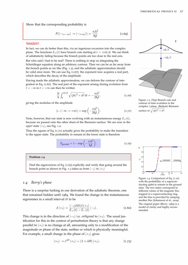
In fact, we can do better than this, via an ingenious excursion into the complexplane. The functions E±(t) have branch cuts starting at t = ±i∆/β. We can thinkof adiabaticity failing because the branch points are too close to the real axis.
But who said t had to be real? There is nothing to stop us integrating theSchrödinger equation along an arbitrary contour. Then we can be as far away fromthe branch points as we like (Fig. 1.3), and the adiabatic approximation shouldbe valid once more. We can use Eq. (1.67): the exponent now acquires a real part,which describes the decay of the amplitude.
Figure 1.3: (Top) Branch cuts andcontour of time evolution in thecomplex t plane. (Bottom) Riemann
surface of√(βt)2 + ∆2
Having made the adiabatic approximation, we can deform the contour of inte-gration in Eq. (1.67). The real part of the exponent arising during evolution fromt = −∞ to t = +∞ can then be written
2ih
∫ i∆/β
0
√(βt)2 + ∆2 dt = −π∆2
2hβ, (1.70)
giving the modulus of the amplitude
|c−(−∞→ +∞)| = exp(−π∆2
2hβ
). (1.71)
Note, however, that our state is now evolving with an instantaneous energy E+(t),because we passed onto the other sheet of the Riemann surface. We are now in theupper state |+t〉, see Fig. 1.2.
Thus the square of Eq. (1.71) actually gives the probability to make the transitionto the upper state. The probability to remain in the lower state is therefore
Pground = 1− exp(−π∆2
hβ
). (1.72)
Problem 1.9
Find the eigenvectors of Eq. (1.65) explicitly and verify that going around thebranch point as shown in Fig. 1.3 takes us from |−t〉 to |+t〉
4
−0.765 −0.76 −0.755 −0.75 −0.745 −0.74 −0.735 −0.73
10−2
10−1
100
Φxcjj (Φ0)
Δ (m
K)
(a)
10−4 10−2 100 102 1040
0.2
0.4
0.6
0.8
1
Δ (mK)
P g
(b)
T
Incoherent Coherent
FIG. 4: (a) Plot of ! vs. flux bias "cjjx applied to the com-
pound junction. The lower curve is ! measured with MRTand the upper curve is ! measured with LZ. (b) Experi-mental (dots) and theoretical (line) ground state probabilityPg = 1 ! PLZ, for fixed ! = 0.05"0/µs as a function of !.The dashed line indicates the crossover between the incoher-ent and coherent regime, defined by W " !.
graph, the theoretical prediction of Eq. (10), using !p andW extracted from the MRT in Fig. 2a, and found verygood agreement with the experiment with no extra fit-ting parameters. At larger biases, |!x,f | > 2.5 m!0, theexperimental " deviates from the theoretical curve dueto tunneling to the first excited state in the target well.
The measurements of the transition rates and the LZprobability allow us to extract " as a function !cjj
x for alarge range of " [18]. Exponential dependence on !cjj
x isevident in Fig. 4a. Figure 4b plots the LZ probability, fora fixed value of #, as a function of " for a quite wide rangeof " (from 27 µK to 1.25 K) together with the theoreticalprediction [19]. In the figure we have identified a line " =W which separates coherent tunneling from incoherenttunneling regime. Excellent agreement with theory isobserved.
We have reported on an experimental probe of thepractically interesting regime for adiabatic quantumcomputation, where the energy gap " is much smallerthan both the decoherence induced energy level broad-ening W and temperature T . The method used iso-
lates a single qubit in a larger-scale adiabatic quan-tum computer, tunes its tunneling amplitude " into the" ! W, T limit, and forces it to undergo a LZ tran-sition. We find that the transition probability for thequbit quantitatively agrees with the theoretical predic-tions. In particular, we demonstrate that in this largedecoherence limit, the quantum mechanical behavior ofthis qubit is the same (except for possible renormaliza-tion of ") as that of a noise-free qubit, as long as the en-ergy bias sweep covers the entire region of broadening W .The close agreement between theory and experiment fora single qubit undergoing a LZ transition in the presenceof noise supports the accuracy of our dynamical models,including both the noise model and the model of a sin-gle superconducting qubit that has been isolated from itssurrounding qubits in an adiabatic quantum computer.Future experiments will test the behavior of multiple cou-pled qubits undergoing a LZ transition in the presence ofnoise.
The authors are grateful to D.V. Averin for fruitfuldiscussions. Samples were fabricated by the Microelec-tronics Laboratory of the Jet Propulsion Laboratory, op-erated by the California Institute of Technology under acontract with NASA.
! Electronic address: [email protected][1] E. Farhi, J. Goldstone, S. Gutmann, J. Lapan, A. Lund-
gren, and D. Preda, Science 292, 472 (2001).[2] D. Aharonov, W. van Dam, J. Kempe, Z. Landau, and
S. Lloyd, SIAM J. Comput. 37, 166 (2007).[3] L.D. Landau, Phys. Z. Sowjetunion 2, 46 (1932).[4] C. Zener, Proc. R. Soc. A 137, 696 (1932).[5] M. Neilson and I. Chuang, Quantum Computation
and Quantum Information, Cambridge University Press(2000).
[6] A.M. Childs, E. Farhi, and J. Preskill, Phys. Rev. A 65,012322 (2001).
[7] M.H.S. Amin, P.J. Love, and C.J.S. Truncik, Phys. Rev.Lett. 100, 060503 (2008).
[8] M.H.S. Amin and D.V. Averin, arXiv:0708.0384.[9] M.H.S. Amin, C.J.S. Truncik, and D.V. Averin,
arXiv:0803.1196.[10] A. Izmalkov, M. Grajcar, E. Il’ichev, N. Oukhanski,
Th. Wagner, H.-G. Meyer, W. Krech, M.H.S. Amin, A.Maassen van den Brink, A.M. Zagoskin, Europhys. Lett.65, 844 (2004).
[11] W.D. Oliver, Y. Yu, J.C. Lee, K.K. Berggren, L.S. Levi-tov, T.P. Orlando, Science 310, 1653 (2005).
[12] M. Sillanpaa, T. Lehtinen, A. Paila, Yu. Makhlin, and P.Hakonen, Phys. Rev. Lett. 96, 187002 (2006).
[13] A.J. Leggett et al., Rev. Mod. Phys. 59, 1 (1987).[14] U. Weiss, “Quantum Dissipative Systems”, World Scien-
tific, Singapore, 2nd edition (1999).[15] P. Ao and J. Rammer, Phys. Rev. B 43, 5397 (1991).[16] M.H.S. Amin and D.V. Averin, Phys. Rev. Lett. 100,
197001 (2008).[17] R. Harris, M.W. Johnson, S. Han, A.J. Berkley, J.
Figure 1.4: Comparison of Eq. (1.72)with the probability of a supercon-ducting qubit to remain in the groundstate. The two states correspond todifferent values of the magnetic fluxtrapped in a superconducting ring,and the bias is provided by rampinganother flux (Johansson et al., 2009).
1.4 Berry’s phase
There is a surprise lurking in our derivation of the adiabatic theorem, onethat remained hidden until 1984. We found the change in the instantaneouseigenstates in a small interval δt to be
The original paper (Berry, 1984) is amodel of clarity and highly recom-mended.
δ |+t〉 =〈−t|δH(t)|+t〉E+(t)− E−(t)
|−t〉 . (1.60)
This change is in the direction of |−t〉 i.e. orthgonal to |+t〉. The usual jus-tification for this in the context of perturbation theory is that any changeparallel to |+t〉 is no change at all, amounting only to a modification of themagnitude or phase of the state, neither or which is physically meaningful.For example, a small change in the phase of |+t〉 gives
|+t〉 → eiδθ |+t〉 ∼ (1 + iδθ) |+t〉 . (1.73)

18 austen lamacraft
Suppose now that H(t) is subject to some adiabatic cyclic change aroundsome closed path γ in the space of matrices. If after time T we have H(T) =H(0), then after evolving |+t〉 according to Eq. (1.60) it would be natural toexpect that it will return to its original value. That is,
|+T〉 ?= |+0〉 . (1.74)
Berry’s remarkable discovery was that this does not happen. Rather,
|+T〉 = eiθB[γ] |+0〉 , (1.75)
where the phase θB[γ] that now bears his name is a functional of the path γ.To get a better grip on this slippery concept, recall that the Hamiltonian of
our two state system (Eq. (1.43)) is parametrized in terms of the field H(t).Suppose we fix the states |H,±〉 for each value of the field at the outset. Thatis, there is no ambiguity in the phase as in Eq. (1.75). We can then use thesestates to write the state of the system in the instantaneous eigenbasis (c.f.Eq. (1.58))
|Ψ(t)〉 = c+(t) |H(t),+〉+ c−(t) |H(t),−〉 . (1.76)
If |H,+〉 changes smoothly as H changes, we will see that Eq. (1.60) cannotbe obeyed: there is always some contribution in the direction of |H,+〉 corre-sponding to a change of phase. This defines a vector field in the space of Hby
A+(H) ≡ −i 〈H,+| (∇H |H,+〉) , (1.77)
and likewise for |H,−〉.
Problem 1.10
Show that using normalized states guarantees that A+(H) is real.
Things become a lot clearer with a concrete example. Let’s write H =
H0n, with n a unit vector. Introducing spherical polar coordinates in theusual way
n =
sin θ cos φ
sin θ sin φ
cos θ
, (1.78)
The Hamiltonian H = H · S takes the form
H =H0
2
(cos θ sin θ e−iφ
sin θ eiφ − cos θ.
)(1.79)
You can then easily check that the eigenstate |H,+〉 is
|H,+〉 =(
cos (θ/2) e−iφ/2
sin (θ/2) eiφ/2
). (1.80)
Computing A+(H) defined by Eq. (1.77) givesThe gradient operator in spherical
polars is ∇ = r ∂r +θr ∂θ +
φr sin θ ∂φ.
We’ll often use the notation ∂x = ∂∂x ,
∂2x = ∂2
∂x2 , etc. in these notes.A+(H) = −φ
cot θ
2r. (1.81)

theoretical physics ii 19
Problem 1.11
By finding |H,−〉, convince yourself that
A−(H) = +φcot θ
2r. (1.82)
We now use Eq. (1.76) in the derivation of the adiabatic theorem as before.Instead of Eq. (1.60) we get
δ |H,+〉 = 〈H,−|δH|H,+〉H0
|H,−〉+ iA+(H) · δH |H,+〉 , (1.83)
where we have used E+ − E− = H0. After making the adiabatic assumptionwe get
ihddt
(c+c−
)=
(E+(t) + hA+(H) · H 0
0 E−(t) + hA−(H) · H
)(c+(t)c−(t)
),
(1.84)and the solution is now
c±(t) = exp(− i
h
∫ t
0
[E±(t′) + hA±(H) · H
]dt′)
c±(0). (1.85)
Moving around a closed loop, we see that the states acquires an additionalphase
θB,±[γ] = −∮
γA±(H) · dH, (1.86)
which depends only on the path, and not on the way it is traversed (i.e. theparametrization H(t)).
Figure 1.5: Sir Michael Berry may bebest known to the general public asthe winner of the 2000 IgNobel prizefor physics, for his work on levitatingfrogs. He shared the prize with AndreGeim, who went on to be the firstperson to win both the IgNobel andNobel prizes (the latter in 20010 for thediscovery of Graphene). Many predictthat Berry will be the next.
Clearly, A± depends on how we chose our states |H,±〉 in the first place.So you could be forgiven for thinking that θB,± does too. However, any otherchoice can be obtained by multiplying |H,±〉 by some H dependent phasefactor. Then
|H,±〉 → exp (iΛ±(H)) |H,±〉A±(H)→ A± +∇HΛ±(H),
(1.87)
and the line integral in Eq. (1.86) is unchanged. Thus θB,α is a property of thepath γ in the H space, not of how the phases of the eigenstates are chosen.
You should recognize Eq. (1.87) as a gauge transformation, with A±(H)
playing the role of the vector potential (sometimes called the Berry poten-tial). We have just shown that θB,± is a gauge invariant quantity.
To get to the geometric meaning of θB,±, we compute the ‘magnetic field’associated with A±
B±(H) ≡ ∇H ×A±(H) = ± r2r2 . (1.88)
which corresponds to a magnetic monopole of charge ± 12 at the origin. This
field is a gauge invariant quantity, which provides another way of seeing thegauge invariance of θB,±. Using Stokes’ theorem to convert the loop integralin Eq. (1.86) into a surface integral over a surface Σ bounded by γ gives While there is an ambiguity of Ω ↔
4π − Ω in the solid angle enclosedby a curve, this is harmless because(accounting for the change in the senseof the curve) it amounts to a change ofthe phase by 2π.
θB,±[γ] = −∫
ΣB± · dS = ∓Ω
2, (1.89)

20 austen lamacraft
where Ω is the solid angle enclosed by Σ.Note that the singularities appearing the gauge field in Eq. (1.81) at the
north and south poles have no physical meaning. It is better to focus on thefield B± which is well behaved there.
TANGENT A beautiful classical analogue of Berry’s phase can be demonstratedusing a gyroscope. Imagine holding one end of its axle, and moving it around sothat a unit vector parallel to the axle traces out a closed curve on the unit sphere.When you return the axle to its original orientation, you will find – provided thebearings are nice and smooth – that the wheel has rotated! Remarkably, the angleof rotation turns out to be the solid angle enclosed within the curve traced out onthe unit sphere.Other discussions of this effect can
be found in (Montgomery, 1991) and(Levi, 1994).
It sounds like this must be connected to Berry’s phase, and indeed it is. Thoughthe physics of this situation is very different, the mathematics is almost identical.To deal with the physics first: the key point is that, by holding the gyroscope bythe axle, we never apply any torque parallel to the axle. Thus the angular momen-tum in this direction is fixed (to zero, say). However, this direction is changing intime.
Let’s denote by θ the angular orientation of the wheel on the axle. Imagine mark-ing out the angle in degree increments on the axle, and measuring θ using somemark on the wheel. It’s natural to write the condition of vanishing angular mo-mentum as
Laxle?= Iθ = 0. (1.90)
Actually, this won’t quite do, because the whole point is that the axle itself is goingto move. Imagine twisting the axle back and forth, keeping it pointing in the samedirection. The wheel will not move, though the angle θ will be going up and downbecause the axle is moving.
To include this effect, imagine defining an orthonormal triad of vectors (a, b, n),where n is parallel to the axle, and a × b = n. The motion we just describedcorresponds to a rotation in the a− b plane. Rotating the axle by φ corresponds to
a→ cos φa + sin φb
b→ cos φb− sin φa.(1.91)
Now notice thatdφ = −a · db = b · da (1.92)
Thus Eq. (1.90) should really be
θ + φ = θ +12[b · a− a · b
]= 0. (1.93)
To make the connection to Berry’s phase, we introduce the complex vector ψ =
(a + ib) /√
2. Then Eq. (1.93) can be written
θ + iψ† dψ
dt= 0. (1.94)
Now for each direction n, fix a and b. We have some freedom here, as we can al-ways choose them differently by rotating in the plane normal to n as in Eq. (1.91).This is entirely analogous to the freedom to choose a gauge that we had in thequantum problem. Once we have done this, we can find the angle of rotation by
∆θ =∫
θ dt =∫−iψ† dψ
dtdt =
∫An · dn, (1.95)
where we defined An = −iψ†∇nψ. Just as with Berry’s phase, this angle isindependent of the arbitrary choice we just made.
Now we just have to compute it. We first fix an explicit form for the triad
a = (cos θ cos φ, cos θ sin φ,− sin θ)
b = (− sin φ, cos φ, 0)
n = (sin θ cos φ, sin θ sin φ, cos θ),
(1.96)

theoretical physics ii 21
and then computeAn = − cos θ∇nφ. (1.97)
We get
∆θ =∮
An · dn =∫
(∇n ×An) · dS =∫
sin θ dθ dφ = Ω, (1.98)
which is the result stated above.
∇n × An can be found in a slicker way without introducing an explicitparametrization of the triad. To evaluate the antisymmetric tensor
∂ia · ∂jb− ∂ja · ∂ib, (1.99)
we first notice that ∂ia must lie in the b− n plane (to preserve normalization) andlikewise ∂jb must lie in the a− n plane. Thus Eq. (1.99) can be written
∂ia · ∂jb− ∂ja · ∂ib = (n · ∂ia)(
n · ∂jb)−(
n · ∂ja)(n · ∂ib) . (1.100)
Now using the property n · ∂ia = −a · ∂in, which follows from preserving theorthogonality of the triad under differentiation, we have
(n · ∂ia)(
n · ∂jb)−(
n · ∂ja)(n · ∂ib) = (a · ∂in)
(b · ∂jn
)−(
a · ∂jn)(b · ∂in)
= (a× b) ·(
∂in× ∂jn)
= n ·(
∂in× ∂jn)
.
(1.101)
In polar coordinates
n ·(
∂in× ∂jn)= sin θ ∂iθ ∂jφ, (1.102)
which is just what we found before.


2Introduction to path integrals
My machines came from too far away.Richard Feynman
2.1 The languages of quantum theory
From the outset, quantum mechanics was written in two apparently differentlanguages. Schrödinger’s equation, published in 1926, describes the timeevolution of the wave function Ψ(r, t) of the system
ih∂Ψ∂t
=
[− h2∇2
2m+ V(r)
]Ψ(r, t). (2.1)
It is historically the second formulation of modern quantum theory, the firsthaving been given a year earlier by Heisenberg. In Heisenberg’s version it Dirac’s book The Pinciples of Quantum
Mechanics (Dirac, 1982), published in1930, is worth opening to marvel athow little the formalism has changedfrom that day to this. To get some ideaof the speed with which these ratherabstract notions had entered physics,bear in mind that Heisenberg’s mentorMax Born had to point out to him thatthe novel rule Heisenberg had foundfor composing matrix elements wasnothing but matrix multiplication, littleused by physicists of the day!
is the matrix elements of observables that evolve in time: hence this way ofdoing things is sometimes known as matrix mechanics. Schrödinger quicklyproved the equivalence of the two approaches, and in Dirac’s formulation ofoperators acting in Hilbert space, this equivalence is rather evident. The evo-lution of a state can be written using the unitary operator of time evolutionU(t) ≡ e−iHt/h, where H is the Hamiltonian, as
|Ψ(t)〉 = U(t) |Ψ(0)〉 . (2.2)
For any operator O and pair of states |Φ〉, |Ψ〉, we then have
〈Ψ(t)|O|Φ(t)〉 = 〈Ψ(0)|O(t)|Φ(0)〉 (2.3)
where O(t) ≡ eiHt/hOe−iHt/h defines the time evolution of O. To put itanother way, O(t) obeys the Heisenberg equation of motion
dOdt
=ih[H,O] . (2.4)
In contrast to the Schrödinger equation, which allowed physicists trained tosolve the partial differential equations of classical physics to go to work onthe problems of the atom, Heisenberg’s formulation is practically useless. Ittook the genius of Wolfgang Pauli to solve the Hydrogen atom using matrixmechanics, a calculation we will discuss in Chapter 6 The original reference is (Feynman,
1948). Coincidentally, around the sametime a fourth formulation of quantumtheory was given by Groenewold andMoyal. This phase space formulationmakes contact with classical mechanicsthrough the Hamiltonian, rather thanLagrangian, viewpoint. We’ll meet itbriefly in Chapter 4.
Eq. (2.1) and Eq. (2.4) embody a radical departure from classical ideas. Inparticular, the notion of a trajectory r(t) of a particle in time is nowhere to beseen. It is surprising, then, that there is a way to describe quantum mechan-ics in terms of trajectories, and more surprising still that it did not emergeuntil more than 20 years after the above formulations. This is Feynman’spath integral.

24 austen lamacraft
2.2 The propagator
The path integral is a tool for calculating the propagator. Since this is anidea of wider utility, we’ll take a moment to get acquainted. In fact, we al-ready have, for the propagator is just a representation of the time evolutionoperatorThe weird notation K(r, t|r′, t) is to
emphasize that r′ and t′ are to betreated as parameters. In particular,when we apply the Hamiltonian, itwill operate on the r variable only.
K(r, t|r′, t′) ≡ θ(t− t′) 〈r|U(t− t′)|r′〉 , (2.5)
where |r〉 denotes a position eigenstate. θ(t) is the step function
θ(t) ≡
1 t ≥ 0
0 t < 0. (2.6)
As the name implies, K(r, t|r′, t′) is used to propagate the state of a systemforward in time. Thus Eq. (2.2) may be written, for t > t′
Ψ(r, t) = 〈r|Ψ(t)〉 = 〈r|U(t− t′)|Ψ(t′)〉
=∫
dr′ 〈r|U(t− t′)|r′〉 〈r′|Ψ(t′)〉
=∫
dr′ K(r, t|r′, t′)Ψ(r′, t′),
(2.7)
where in the second line we inserted a complete set of states. Equivalently,K(r, t|r′, t′) is the fundamental solution of the time dependent Schrödingerequation, which means that it satisfies[
ih∂
∂t− H
]K(r, t|r′, t′) = ihδ(r− r′)δ(t− t′) and
K(r, t|r′, t′) = 0 for t < t′(2.8)
Problem 2.1
Explain why these two definitions are equivalent. Hint: integrateEq. (2.8) through a small interval t′ − ε < t < t′ + ε to findK(r, t′ + ε|r′, t′).
The idea of representing the solution of a partial differential equation (PDE)should be familiar to you from your study of Green’s functions. Indeed,‘Green’s function’ and ‘propagator’ are often used interchangeably.
The fact that the wavefunction at later times can be expressed in terms ofΨ(r, 0) is a consequence of the Schrödinger equation being first order in time(and linearity naturally implies the relationship is a linear one). To see thegenerality of the idea, let us first discuss how it works for the heat equation,another PDE first order in time. The fundamental solution satisfies[
∂
∂t− D∇2
r
]Kheat(r, t|r′, t′) = δ(r− r′)δ(t− t′)
Kheat(r, t|r′, t′) = 0 for t < t′(2.9)

theoretical physics ii 25
Problem 2.2
Show (i.e. verify – if you have the answer already that’s perfectly ac-ceptable!) that the fundamental solution of the heat equation is
Kheat(r, t|r′, t′) =θ(t− t′)
(4πD(t− t′))3/2 exp[− (r− r′)2
4D(t− t′)
](2.10)
Thus if Θ(r, 0) describes the initial temperature distribution within a uni-form medium with thermal diffusivity D, then at some later time we have
Θ(r, t) =∫
dr′ Kheat(r, t|r′, 0)Θ(r′, 0). (2.11)
Eq. (2.10) and Eq. (2.11) have the following meaning. We can represent theinitial continuous temperature distribution as an array of hot spots of vary-ing temperatures. The evolution of a hot spot is found by solving Eq. (2.10),with the right hand side representing a unit amount of heat injected intothe system at point r′ and time t′. As time progresses, each hot spot diffusesoutwards with a Gaussian profile of width
√D(t− t′), independently of the
others by virtue of the linearity of the equation.
Figure 2.1: Spreading of a hot spot.
Problem 2.3
What can be accomplished in one time step can equally well be done intwo. The propagator must have the property
K(r, t|r′, t′) =∫
dr′′ K(r, t|r′′, t′′)K(r′′, t′′|r′, t′). (2.12)
Verify that this holds for Kheat(r, t|r′, t′).
With this in hand, it’s a small leap to find the propagator for the freeparticle Schrödinger equation. The Hamiltonian is H = − h2∇2
2m , so by takingD → h
2m and t→ it, we get In d dimensions the 3/2 power in theprefactor becomes d/2.
Kfree(r, t|r′, t′) = θ(t− t′)(
m2iπh(t− t′)
)3/2exp
[−m(r− r′)2
2ih(t− t′)
](2.13)
The propagator in momentum space
We originally defined the propagator in Eq. (2.5) as a real space repre-sentation of the time evolution operator. We could just as well choose totake matrix elements in another basis. Since the free particle HamiltonianH = − h2∇2
2m is diagonal in momentum space, it makes sense to look at Don’t forget that with the normal-ization used here, |r〉 has units of[Length]−d/2, while |p〉 has units[Momentum]−d/2. A δ-function δ(x) ind-dimensions has units of [x]−d.
Kfree(p, t|p′, t′) = θ(t− t′) 〈p|U(t− t′)|p′〉
= θ(t− t′) exp(−i
p2
2mt− t′
h
)δ(p− p′)
(2.14)

26 austen lamacraft
Problem 2.4
Confirm that Eq. (2.13) and Eq. (2.14) are related by a change of basis(Fourier transform) using
〈r|p〉 = exp(ip · r/h)
(2πh)3/2 .
Notice that the reproducing property (Problem 2.3) is trivial in thisbasis.
This idea generalises to any time independent Hamiltonian with a com-plete set of energy eigenfunctions ϕα(r) and eigenvalues Eα
K(r, t|r′, t′) = θ(t− t′)∑α
ϕα(r)ϕ∗α(r′)e−iEα(t−t′)/h. (2.15)
For a time dependent Hamiltonian, we have the complication that the timeevolution operator must be thought of as a function of two variables – theinitial and final times, say – rather than just the duration of evolution.In terms of the Hamiltonian H(t),
U(t, t′) has the deceptively simpleform
U(t, t′) = T exp[− i
h
∫ t
t′dti H(ti)
],
where T denotes the time orderingoperator. The time ordering is essentialbecause the commutator of the Hamil-tonian evaluated at two different timesis in general nonzero.
|Ψ(t)〉 = U(t, t′) |Ψ(t′)〉 . (2.16)
Nevertheless, the propagator K(r, t|r′, t′) = θ(t− t′) 〈r|U(t, t′)|r′〉 obeys thesame basic equation Eq. (2.8).
2.3 The path integral
By using the reproducing property of the kernel (Problem 2.3) we can sub-divide the evolution from time ti to tf into N smaller intervals of length∆t = (tf − ti) /N, each characterized by its own propagator
r
tf
ri
rf
ti
Figure 2.2: Slicing the propagationtime into many small intervals.
K(rf, tf|ri, ti) =∫
dr1 · · · drN−1 K(rf, tf|rN−1, tN−1) · · ·K(r1, t1|ri, ti). (2.17)
This is not totally perverse: as we will see shortly the apparent increase incomplexity is countered by the simplification of the propagator for smallpropagation intervals. The idea is that in the limit1 the integration over the1 These three words are terribly glib.
Spare a thought for the mathemati-cians who had to try and make some-thing respectable out of this!
variables ri becomes an integral over paths r(t), with a continuous index –time – rather than a discrete one. This is the path integral.
So what is the integrand? A clue is provided by the observation that inthe presence of a constant potential V(r) = V0, the propagator is a simplemodification of Eq. (2.13)
Kfree(r, t|r′, t′) = θ(t− t′)(
m2iπh(t− t′)
)3/2exp
[−m(r− r′)2
2ih(t− t′)− i
V0(t− t′)h
],
(2.18)as may be verified by direct substitution into the Schrödinger equation. Nowas the propagation time t− t′ goes to zero, we know that the propagator isgoing to approach a δ-function. Therefore, Eq. (2.18) should still hold if wetake V0 to be the value of the potential at the midpoint r+r′
2 (say)2.2 The particular choice is unimportanthere, but the midpoint prescriptionturns out to be vital when a vectorpotential is included. See (Schulman,2005), Chapter 4.
Putting this into Eq. (2.17), for N → ∞, (ri+1 − ri)2/(ti+1 − ti)→ r2∆t,
K(rf, tf|ri, ti) =∫
r(tf)=rfr(ti)=ri
Dr(t) exp(
ih
∫ tf
ti
[mr2
2−V(r(t))
]dt)
. (2.19)

theoretical physics ii 27
The symbol Dr(t), which corresponds to a ‘volume element’ in the spaceof paths, is presumed to contain the appropriate normalization, including ahorribly divergent factor
( m2iπh∆t
)3N/2. The subscript on the∫Dr(t) integral
indicates that all paths must begin at ri and end at rf.One may wonder how Eq. (2.19), beset by such mathematical vagaries, can
be of any use at all. One thing we have going for us is that all of these diffi-culties have nothing to do with V(r), and are therefore unchanged in goingfrom the free particle case to something more interesting. We can thereforeuse the free particle result to provide the normalization, and calculate theeffect of introducing V(r) relative to this.
Enter the Lagrangian
It’s a historical oddity that the Hamiltonian is one of the last things you meetin classical mechanics and one of the first in quantum mechanics. Eq. (2.19)represents the first appearance in quantum mechanics of the Lagrangian
L(r, r) ≡ mr2
2−V(r), (2.20)
and its time integral, the action The square brackets are used toindicate that S is a functional of thepath. A functional is a machine thattakes a function and produces anumber.
S[r(t)] ≡∫ tf
ti
L(r(t), r(t)) dt (2.21)
As you know very well, variations of the path r(t) with fixed endpoints (i.er(ti) = ri, r(tf) = rf) leave the action unchanged to first order if (and only if)the Euler–Lagrange equations are satisfied
∂L∂r− d
dt
(∂L∂r
)= 0. (2.22)
As we’ll see shortly, the path integral provides a natural explanation of howthese equations and the action principle arise in the classical limit.
2.4 Path integral for the harmonic oscillator
To show that this all works we at least have to be able to solve the harmonicoscillator. Confining ourselves to one dimension, the Lagrangian is
LSHO(x, x) =12
mx2 − 12
mω2x2. (2.23)
The propagator is therefore expressed as the path integral
KSHO(xf, tf|xi, ti) =∫
x(tf)=xfx(ti)=xi
Dx(t) exp
(ih
SSHO[x(t)]︷ ︸︸ ︷∫ tf
ti
[mx2
2− mω2x2
2
]dt
). (2.24)
This form is reminiscent of a Gaussian integral. Before we can use this in-sight, we first have to deal with the feature that the paths x(t) satisfy theboundary conditions x(ti) = xi, x(tf) = xf. We can make things simplerby substituting x(t) = x0(t) + η(t), where x0(t) is some function satisfy-ing these same conditions. Then η(t), the new integration variable, satisfiesη(ti) = η(tf) = 0.
28 austen lamacraft
What should we take for x0(t)? Making the substitution in the actiongives A linear shift x(t) = x0(t) + η(t) does
not effect the integration element:Dx(t) = Dη(t)
SSHO[x0(t) + η(t)] = SSHO[x0(t)] + SSHO[η(t)]
+∫ tf
ti
[mx0(t)η(t)−mω2x0(t)η(t)
]dt. (2.25)
Integrating the last term by parts, and bearing in mind that η(t) vanishes atthe endpoints, puts it in the form
−∫ tf
ti
[mx0(t) + mω2x0(t)
]η(t) dt. (2.26)
We recognize the quantity in square brackets as the equation of motionof the simple harmonic oscillator. Thus if we choose x0(t) to satisfy thisequation, the cross term in Eq. (2.25) vanishes and the propagator takes theformChoosing x0(t) to be the classical
trajectory eliminates the linear term inη in general. This is after all exactlywhat the action principle tells usthat classical trajectories do (note thecondition of fixed endpoints, vital inthe derivation of the Euler–Lagrangeequations, arises naturally here). Theaction for η(t) will not be independentof x0(t) for more complicated – i.e.non-quadratic – Lagrangians, however.
KSHO(xf, tf|xi, ti) = exp(
ih
SSHO[x0(t)])×∫
η(tf)=η(ti)=0Dη(t) exp
(ih
∫ tf
ti
[mη2
2− mω2η2
2
]dt)
. (2.27)
Problem 2.5
Show that the classical action is
SSHO[x0(t)] =mω
2 sin [ω (tf − ti)]
[(x2
i + x2f
)cos [ω (tf − ti)]− 2xixf
](2.28)
Now we turn our attention to the η path integral in Eq. (2.27). Because theaction for η(t) is independent of time, and η(t) vanishes at the endpoints, itcries out to be expanded in a Fourier series
η(t) =∞
∑n=1
ηn sin[
πn (t− ti)
tf − ti
]. (2.29)
In terms of the Fourier coefficients ηn the action takes the form
SSHO[η(t)] =m (tf − ti)
4
∞
∑n=1
[π2n2
(tf − ti)2 −ω2]
η2n. (2.30)
The η integral now begins to look like a product of Gaussian integrals, pro-vided that we are free to interpret Dη(t) = ∏∞
i dηn (we are).The Gaussian integral we can do
∫ ∞
−∞dx e−bx2/2 =
√2π
b. (2.31)
So we take a wild guess and write
KSHO(xf, tf|xi, ti)?= exp
(ih
SSHO[x0(t)])×
∞
∏n=1
√4πih
m(tf − ti)
π2n2 −ω2(tf − ti)2 .
(2.32)

theoretical physics ii 29
Does it work? No. But then we didn’t expect it to, because of the difficultiesin defining the path integral in the first place. However, as we noted in theThe mathematically temperate will
recoil at using Eq. (2.31) with imag-inary b. The solution is to rotate thecontour of the time integral in theaction slightly counterclockwise inthe complex plane, so that the (tf − ti)factor at the front of Eq. (2.29) becomes(tf − ti + iε), for some infinitesimal ε.This is enough to guarantee conver-gence of the integral without changingthe result.
previous section, the fudge factor required is independent of the potential,so the overall normalization can be deduced from the free particle result thatmust apply when ω = 0. Adapting the result Eq. (2.13) to one dimension, wefind
KSHO(xf, tf|xi, ti) =
(m
2iπh(tf − ti)
)1/2exp
(ih
SSHO[x0(t)])
×∞
∏n=1
(1− ω2(tf − ti)
2
π2n2
)−1/2
. (2.33)
The infinite product was found by Leonhard Euler (1707-1783)
∞
∏n=1
(1− ω2(tf − ti)
2
π2n2
)=
sin ω(tf − ti)
ω(tf − ti). (2.34)
We arrive at the final result
KSHO(xf, tf|xi, ti) =
(mω
2iπh sin ω(tf − ti)
)1/2exp
(ih
SSHO[x0(t)])
.
(2.35)
Problem 2.6
Show that this is correct. Hint: You only need to show that this solvesthe appropriate Schrödinger equation, as the short time behaviour(when ω(tf − ti) 1) is the same as for the free particle.
What can you actually do with a path integral?
• Gaussian integrals (like the simple harmonic oscillator).
• Err...
• That’s it.
Bear in mind, however, that the number of problems that can be solvedexactly by the other formulations of quantum mechanics is also rather lim-ited. Apart from the harmonic oscillator, the other Hamiltonian you all knowhow to solve exactly is the Hydrogen atom. Can it be done with a path inte-gral? The answer is yes3. Furthermore, the special features of the Hydrogen 3 I.H. Duru and H. Kleinert. Physics
Letters B, 84(2):185–188, 1979atom that make it amenable to exact solution – we’ll discuss them in Chap-ter 6 – are precisely the same features that make it possible to calculate thepath integral. This illustrates the principle of conser-
vation of troubles, according to whicha problem is no easier or harder in adifferent language; the difficulties arejust moved around (and sometimes outof sight!).
The value of the path integral is firstly to provide a new language forquantum theory, one that has given rise to many new insights. New effectscan arise when the topology of paths is important, e.g. the Aharonov–Bohmeffect.
A new formulation can also suggest new approximate methods to solveproblems that have no exact solution. The most obvious approach is to ex-pand the integrand in the path integral in powers of the potential V(r). This

30 austen lamacraft
turns out to be equivalent to time-dependent perturbation theory, as you caneasily check.
A more useful line of attack is to try to evaluate the path integral numer-ically, using the same discretization of time that we used to derive it. ForEq. (2.19) this is in fact a terrible idea, as the integrand is complex, and os-cillates wildly, leading to very poor convergence. However, as we’ll see inChapter 4, it is possible to formulate the partition function of quantum sta-tistical mechanics as a path integral in imaginary time. We’ve already seenthe form of the propagator in imaginary time, when we discussed the heatequation (Eq. (2.10)). Notice that it is real and positive, so we can think of itas a probability distribution. Evaluating the partition function by samplingthe probability distribution of paths is the basis of the path integral MonteCarlo method.
2.5 The method of stationary phase
The other great insight provided by the path integral concerns the emer-gence of classical mechanics from quantum mechanics. The appearance ofthe Lagrangian and action in the integrand should already have us askingwhat role the condition of stationary action plays in quantum theory. A clueis provided by a method of approximating ordinary integrals that goes bythe names steepest descent, stationary phase, saddle point, or occasionallyLaplace’s method.
As a concrete example, recall that in developing the (J)WKB method, weneed to understand the solutions of Airy’s equationYou may need to look back at AQP
to refresh your memories here. Theidea is that the WKB form of thewavefunction breaks down near theturning points of the classical motion,so one instead approximates thepotential by a straight line, and usesthe exact solution of the Schrödingerequation in a linear potential in thisregion.
f ′′(x)− x f (x) = 0, (2.36)
The solution of this equation is a non-elementary function called the Airyfunction (in fact, there are two linearly independent solutions, as this is asecond order equation), and we are particularly interested in its behaviourat large |x|. As is often the case with special functions, there is an integralrepresentation of the Airy function, and we can use this to find the large |x|behaviour in a controlled way.
The first thing to note is that the Fourier transform of the equationUsing the convention f (x) =∫ ∞−∞ eikx f (k) dk
2π . Overall numericalfactors aren’t important here: it’s alinear equation.
i f ′(k) + k2 f (k) = 0 (2.37)
is first order, and may be solved easily
f (k) = A exp(
ik3/3)
, (2.38)
with A some constant. Thus all we have to do to find the solution f (x) iscompute the Fourier integral
f (x) =∫
eikx f (k) dk = A∫
exp(
ik3/3 + ikx)
dk. (2.39)
But wait! A linear second order equation has two independent solutions,and it looks like we have only found one. However, we didn’t yet specify thecontour of integration in Eq. (2.39), and our freedom to choose this allows usto generate more than one solution.

theoretical physics ii 31
Problem 2.7
Show that f (x) defined by Eq. (2.39) satisfies Airy’s equation as long asthe integrand vanishes at the endpoints. Hint: integrate by parts.
Figure 2.3: A possible contour in theplane of complex k, passing throughone of the stationary points of theintegrand.
Where does the integrand vanish? We have to go to large |k| in such away that the dominant term ik3/3 term in the exponent has a negative realpart. Writing k = |k|eiθ , we can see that this happens as |k| → ∞ in the threewedges
I: 0 < θ < π/3
II: 2π/3 < θ < π
III: 4π/3 < θ < 5π/3
(2.40)
Different choices for the starting and ending wedge give different solutions. Use Cauchy’s theorem to convinceyourself that only two are indepen-dent.
Now comes the key idea. Because the integrand is an exponential, itquickly becomes negligible as we move off into a wedge. The largest con-tribution should come from the largest value of the real part of the exponent.The stationary points satisfy k2 + x = 0 and lie at Why do we look at a stationary point
if we only want to maximize the realpart of the exponent? Think about theCauchy–Riemann equations.ksp =
±i√
x for x > 0
±√|x| for x < 0
, (2.41)
with the integrand taking the values
exp(
ik3sp/3 + ikspx
)=
exp(∓ 2
3 x3/2)
for x > 0
exp(∓i 2
3 |x|3/2)
for x < 0.(2.42)
As we go to large |x|, the decay of the integrand as we move away fromthese stationary points becomes more rapid. Fixing x > 0 and expanding theexponent around the saddle point value gives For an analytic function, all stationary
points are saddle points, which is whywe use the terms interchangeably here.
exp(
ik3/3 + ikx)∼ exp
(∓2
3x3/2
)exp
(∓√
x(k− ksp
)2)
(2.43)
where the ± signs correspond to the stationary points at ±i√
x. For i√
x,moving parallel to the real axis therefore corresponds to the direction ofsteepest descent, in which the integrand decays fastest. For −i
√x, the steepest
descent direction is parallel to the imaginary axis.Eq. (2.43) replaces the integrand by a Gaussian of width ∼ x−1/4, an
approximation that obviously improves very quickly as x becomes large. Forthe contour in Fig. 2.3 which passes through i
√x, the integral in Eq. (2.39) is
then approximately
f (x) ∼ Aπ1/2
x1/4 exp(−2
3x3/2
), as x → ∞. (2.44)
The Airy function Ai(x) is defined by this contour, with the (arbitrary)choice A = 1/ (2π). Thus we have The second solution that grows ex-
ponentially for x → ∞ is denoted byBi(x) and sometimes hilariously calledthe Bairy function.Ai(x) ∼ 1
2π1/2x1/4 exp(−2
3x3/2
), as x → ∞ (2.45)
The case of x < 0 is slightly trickier, as the two stationary points lie onthe real axis. In this case we pass through both stationary points, and in the

32 austen lamacraft
Gaussian approximation we can just sum the contribution from each. Nearthese points the integrand takes the form (c.f. Eq. (2.43))
exp(
ik3/3 + ikx)∼ exp
(∓i
23|x|3/2
)exp
(±i√|x|(k− ksp
)2)
. (2.46)
Figure 2.4: For x < 0 we pass throughboth stationary points of the integrand.
We see that the steepest descent directions are now at angle ±π/4 to thereal axis for the saddle point at ±
√|x|. Accounting for this rotation of the
contour when we do the Gaussian integral gives
Ai(x) ∼ 1π1/2|x|1/4 sin
(23|x|3/2 +
π
4
), as x → −∞. (2.47)
The π/4 phase shift is the ultimate origin of the ‘extra’ 1/2 in the Bohr–Sommerfeld quantization condition∮
p(x)dx = h(
n +12
), n integer, (2.48)
where p(x) =√
2m (E−V(x)) is the classical momentum at position x of aparticle with energy E moving in a potential V(x).
Problem 2.8
You are familiar with Stirling’s approximation in the form
ln N! ∼ N ln N − N. (2.49)
Sometimes, however, this approximation doesn’t cut it. Think of thenumber of ways of getting 50 heads with 100 coin tosses(
10050
)(12
)100=
100!
(50!)2
(12
)100. (2.50)
Eq. (2.49) would tell you that the answer is approximately one. To getsomething better, we write
N! =∫ ∞
0xNe−x dx (2.51)
(proof by integration by parts) and use the saddle point method, validat large N. Show that this yields
N! ∼ NNe−N√
2πN. (2.52)
A better estimate for the above probability is then 15√
2π∼ 0.080.
2.6 The classical limit
Now we understand the method of stationary phase, we proceed to discussthe path integral by analogy. The integrand in Eq. (2.19) is
exp(
ih
S[r(t)])
, (2.53)
where S[r(t)] is the action. Planck’s constant immediately presents itself as asmall parameter on which to base the stationary phase approximation. More

theoretical physics ii 33
precisely, if the ratio of typical variations of the action to Planck’s constant islarge, we are justified in approximating the path integral as Gaussian in thevicinity of the extremum of the action. But we know that the extremum cor- Such approximations are usually called
semiclassical. The WKB method isanother example.
responds to the classical trajectory rcl(t). This suggests that, schematically,the propagator can be written approximately as
K(r, t; r′, t′) ∼ (Gaussian integral)× exp(
ih
S[rcl(t)])
. (2.54)
The classical trajectory is the one satisfying rcl(t) = r, rcl(t′) = r′. That is, theendpoints fix the solution, rather than the initial position and velocity.
The result is a beautiful connection between the classical and quantumformalisms. The path integral tells us that the amplitude of a process is thesum of amplitudes for all possible trajectories between two points. But inthe classical limit – which corresponds to systems sufficiently large that thevariations of the action are much larger that Planck’s constant – almost all ofthese trajectories cancel out because of the wild fluctuations of the phase ofthe integrand. The dominant contributions are those close to the extremumof the integrand i.e. the classical trajectory.
TANGENT Unfortunately we don’t have time to make Eq. (2.54) precise. The resultof evaluating the Gaussian path integral is the van Vleck propagator4. In three 4 See (Van Vleck, 1928). As the date
indicates, you don’t need the pathintegral to derive this result!
dimensions, this is
KvV(r, t; r′, t′) = ∑classical paths
(1
2πih
)3/2det
(− ∂2S
∂r ∂r′
)−1/2
exp(
ih
S[rcl(t)])
.
(2.55)The classical action is a function (not a functional) of r, r′ because rcl(t) dependson the endpoints (c.f. Eq. (2.28)). In general there may be more than one classicaltrajectory connecting two points (if there is periodic motion, say), so we have tosum over all of them, just as when we evaluated the Airy function for x < 0. This doesn’t happen for the harmonic
oscillator because the period is con-stant.


3Scattering theory
Scattering experiments play a vital role in modern physics. In a typical scat-tering experiment, particles approach each other ‘from infinity’ – which is tosay from far outside the range of their interaction with each other – spenda short time in close proximity, and then go their separate ways. As theypropagate outwards from the collision region, their interaction ceases but itsimprint is left on the scattered waves, ready to be picked up by a detector.
This basic picture encompasses a wide variety of different situations. Welist just a few examples
• The scattering of neutrons from a crystal lattice to determine magneticstructure.
• The scattering of α-particles from the nuclei in a layer of gold leaf(Rutherford scattering1). 1
‘It was quite the most in-credible event that has everhappened to me in my life.It was almost as incredibleas if you fired a 15-inch shellat a piece of tissue paperand it came back and hityou.’
• The collision of protons in the LHC.
The usefulness of scattering as an experimental technique therefore hingeson solving the ‘inverse problem’ of inferring the interactions (i.e. the Hamil-tonian) from the scattered waves. Our purpose in this chapter, on the otherhand, is to describe the general mathematical structure of scattering.
3.1 Scattering in one dimension
A great many of the concepts of scattering theory can be introduced in onedimension, where certain complexities of our three dimensional world areabsent. As an additional simplification, we’ll study the scattering of particlesfrom a static potential: the ‘target’. The generalization to the scattering ofpairs of particles is not difficult – it involves viewing the collision in thecentre of mass frame, which as usual reduces to a single particle problem.
Figure 3.1: Schematic view of scatter-ing in one dimension.
The situation we aim to describe is illustrated in Fig. 3.1. A wavepacketapproaches the origin from −∞. Near the origin it interacts with a potentialV(x). As a result of this interaction, a modified wavepacket is transmittedand another is reflected, and these move to ±∞.
Let’s suppose that V(x) either vanishes outside some finite region thatincludes the origin, or is otherwise negligible (exponentially decaying, say).We’ll sometimes refer to this region as the interaction region. Long range po-tentials bring certain complications that need not concern us at the moment.As well as being relevant to a great many scattering experiments, interactionwith a localized potential brings the wonderful simplification that outside of

36 austen lamacraft
the range of the potential, the energy eigenstates of the system take the formof plane waves. This allows us to construct the incoming wavepacket fromthe eigenstates, just as we would construct one from plane waves. If we nowimagine the wavepacket becoming more extended in real space, then eventu-ally it becomes indistinguishable from an eigenstate. In a little while, a ‘relic’of the wavepacket picture will be required to make sense of some of our ex-pressions, but for the moment let us continue to discuss the eigenstates ofthe problem.
As we have already mentioned, outside of the interaction region an en-ergy eigenstate must have the form
Ψk(x) =
a+ exp (ikx) + a− exp (−ikx) x 0
b+ exp (ikx) + b− exp (−ikx) x 0,(3.1)
where the wavevector k is related to the energy of the state by Ek ≡ h2k2
2m .Now, the four complex coefficients in Eq. (3.1) are not independent of eachother. Rather, they are related by finding the form of the wavefunctionwithin the interaction region, as the following example shows.
Problem 3.1
For a δ-function potential V(x) = gδ(x), show that the relationshipbetween the coefficients in Eq. (3.1) may be written in terms of thescattering matrix S(k)
(a−b+
)=
S(k)︷ ︸︸ ︷(rLL tRL
tLR rRR
)(a+b−
), (3.2)
where the reflection and transmission coefficients have the form
rLL = rRR =g
ih2k/m− g, tRL = tLR =
ih2k/mih2k/m− g
. (3.3)
Hint: think about the boundary conditions obeyed by the wavefunctionat the origin.
What property of this problem is responsible for rLL = rRR, tRL =
tLR?
The scattering matrix expresses the outgoing waves (i.e. the wave at x < 0moving to the left and the wave at x > 0 moving to the right) in terms of theincoming waves. Probably you are familiar with the form
Ψk(x) =
exp (ikx) + rLL exp (−ikx) x 0
tLR exp (ikx) x 0, (3.4)
which describes a wave coming in from −∞ only, and corresponds to takinga+ = 1, b− = 0.
Another way to encode the same information is in terms of the transfermatrix T(k), which expresses the amplitudes on one side of the scatterer interms of those on the other(
b+b−
)= T(k)
(a+a−
)=
(tLR − rRRrLL/tRL rRR/tRL
−rLL/tRL 1/tRL
)(a+a−
)(3.5)

theoretical physics ii 37
The transfer matrix has the nice feature that it can be found for a number ofscatterers in series by multiplying together the transfer matrices for each.
The scattering matrix S(k) exists for any potential V(x), being defined bythe relation Eq. (3.2) between the coefficients of the plane wave componentsof an eigenstate outside of the interaction region. It reduces the number ofindependent components in Eq. (3.1) from four to two. The goal of scat- When V(x) = 0 these two independent
solutions can of course be taken to bethe left and right moving waves.
tering theory is to find S(k) given V(x), or at least to deduce its generalproperties. Let us discuss some of these properties now.
Flux conservation and unitarity of S(k)
The probability density P(x, t) = |Ψ(x, t)|2 obeys the continuity equation
∂tP(x, t) + ∂x j(x, t) = 0, (3.6)
where the probability current is
j(x, t) = − ih2m
[Ψ∗∂xΨ−Ψ∂xΨ∗] . (3.7)
When we consider an eigenstate (a.k.a. stationary state), the probability den-sity does not change in time, and we must have
∂x j(x) = 0. (3.8)
If we integrate over a region [−L, L] containing the interaction region, we get
j(−L) = j(L). (3.9)
At x = ±L, we can use the form of the wavefunction from Eq. (3.1), giving
hkm
[|a+|2 − |a−|2
]=
hkm
[|b+|2 − |b−|2
](3.10)
(happily the cross terms vanish). Eq. (3.10) has a straightforward physicalmeaning. ± hk
m is the velocity of a particle described by a plane wave e±ikx,and the contribution of a plane wave to the probability current is the productof the velocity and the (spatially constant) probability density.
Problem 3.2
Show that Eq. (3.10) implies that S(k) is a unitary matrix. Check thatEq. (3.2) is unitary. What is the corresponding condition satisfied byT(k)?
Channels and phase shifts
The scattering matrix, like any unitary matrix, can be diagonlized by a uni-tary transformation U. The eigenvalues are complex numbers of unit magni-tude, so we can write
USU† =
(exp (2iδ1) 0
0 exp (2iδ2)
), (3.11)

38 austen lamacraft
which defines the phase shifts δ1,2. This means that if we express the ampli-tudes in Eq. (3.1) as (
a+b−
)= U†
(cin
1cin
2
)(
a−b+
)= U†
(cout
1cout
2
),
(3.12)
then the new amplitudes cin,out1,2 are related by
cout1,2 = exp (2iδ1,2) cin
1,2. (3.13)
In this way an eigenstate is written as a linear combination of two scatteringchannels, each of which has particular simple scattering properties: there isno ‘mixing’ between channels.
In one dimension by far the most important example is provided by par-ity symmetric potentials V(x) = V(−x). We know that the energy eigen-states of such potentials can be chosen to have a definite parity. Referringto the general form Eq. (3.1), this means that a+ = ±b−, a− = ±b+, witha + sign for an even state and a − for an odd one. In this case we can writeEq. (3.12) asFor V(x) = 0, this corresponds to
working with cos(kx) and sin(kx)instead of e±ikx .
(a+b−
)=
1√2
(1 −11 1
)(cin
evencin
odd
)(
a−b+
)=
1√2
(1 −11 1
)(cout
evencout
odd
).
(3.14)
In this basis Eq. (3.1) takes the form
Ψk(|x| 0) = ceven cos (k|x|+ δeven) + sgn(x)codd cos (k|x|+ δodd) , (3.15)
where for convenience we have defined ceven,odd =
exp(iδeven,odd
)cin
even,odd/√
2
Problem 3.3
Find δeven and δodd for the δ-function potential of Problem 3.1, and theform of the corresponding wavefunctions.
Integral equation for scattering amplitudes
All this formalism is well and good, but how do we find S(k), δ1,2(k), and soon in general? We are looking for solutions of the Schrödinger equation
− h2
2m∂2
xΨ(x) + V(x)Ψ(x) = EkΨ(x), (3.16)
but we know that in general there are two independent solutions at each k,so we need to somehow ‘force’ the solution to be of the form Eq. (3.4) (say)corresponding to a wave coming from −∞. From the solution we can thenread off the scattering amplitudes.
The way to force the solution is to express the wavefunction as
Ψk(x) = exp (ikx) + Ψscattk (x). (3.17)

theoretical physics ii 39
This defines Ψscattk (x), the scattered wave, as the part of the solution that
owes its existence to V(x), and which therefore vanishes as V(x) vanishes.For Eq. (3.4), Ψscatt
k (x) has the explicit form
Ψscattk (x) =
rLL exp (−ikx) x 0
(tLR − 1) exp (ikx) x 0. (3.18)
With the definition Eq. (3.17), we can rewrite Eq. (3.16) as[Ek +
h2
2m∂2
x
]Ψscatt
k (x) = V(x)Ψk(x). (3.19)
Now let’s introduce the inverse of the operator on the left hand side. That is,a function satisfying [
Ek +h2
2m∂2
x
]Gk(x, x′) = δ(x− x′) (3.20)
(This is just the Green’s function of the operator of the free problem, hencethe notation). We’ll write down Gk(x, x′) in a moment, but for now let’s useit to rewrite Eq. (3.19) as
Ψscattk (x) =
∫dx′ Gk(x, x′)V(x′)Ψk(x′). (3.21)
In terms of Ψk(x) this is
Ψk(x) = exp (ikx) +∫
dx′ Gk(x, x′)V(x′)Ψk(x′). (3.22)
Thus we have passed from a differential equation to an integral equation,known as the Lippmann–Schwinger equation. What did we gain by doingthis? The point is that once Gk(x, x′) is given we have an explicit equationwith nothing further to be specified. In particular, there are no boundaryconditions that have to be imposed en route to a unique solution, as is thecase when we solve a differential equation. This is because the choice ofboundary conditions fixes the Green’s function uniquely, as we’ll see in amoment.
Indeed, the most simple-minded way to go about solving Eq. (3.22) is byiteration
Ψk(x) = exp (ikx) +∫
dx′ Gk(x, x′)V(x′) exp(ikx′
)+∫
dx′dx′′ Gk(x, x′)V(x′)Gk(x′, x′′)V(x′′) exp(ikx′′
)+ · · · , (3.23)
which generates the Born series.Now let’s discuss the Green’s function. From Eq. (3.20) we can see that
this satisfies the free particle Schrödinger equation with energy Ek whenx 6= x′. Therefore it has the form
Gk(x, x′) =
g<+ exp (ikx) + g<− exp (−ikx) x < x′
g>+ exp (ikx) + g>− exp (−ikx) x > x′.(3.24)
To fix the form uniquely we specify:
• Gk(x, x′) is continuous at x = x′

40 austen lamacraft
• At x = x′ the derivative jumps
∂xGk(x, x′)|x=x′+εx=x′−ε =
2mh2 . (3.25)
These two conditions follow from the defining Eq. (3.20).
• In order to generate a solution of the form Eq. (3.4), we must have
g<+ = g>− = 0, (3.26)
which corresponds to only ‘outgoing’ waves being generated by the scat-tering potential.If you are uncomfortable with the so-
lution of a time independent equationbeing described as coming or goinganywhere, don’t worry. We’ll return tothe time dependent view of scatteringlater.
Imposing these conditions gives
G+k (x, x′) = −i
mh2k
exp(ik|x− x′|
). (3.27)
We have added a + to indicate this is a particular Green’s function obeyingcertain boundary conditions – the reason for this notation will become clearlater. Because it enshrines the notion of ‘cause’ (the scatterer) preceeding‘effect’ (the outgoing wave), G+
k is called the retarded or causal Green’sfunction.We spoke earlier about imposing
boundary conditions on the Green’sfunction, but didn’t write any explic-itly. That’s because they look slightlyunusual:
lim|x−x′ |→∞
[∂|x−x′ | − ik
]G(x, x′) = 0.
However, this radiation condition hasthe same content as Eq. (3.26).
Problem 3.4
Solve the Lippmann–Schwinger equation for the case of the δ-functionpotential and show that the result of Problem 3.1 is reproduced.
to bend the trajectories of electrons traveling between twoQPCs, they achieved glimpses into the spatial details ofelectron flow in 2DEG nanostructures. Those early exper-iments set the scene for more recent high-resolution im-ages that revealed surprising and important details aboutelectron flow in 2DEGs.
At Harvard, we used scanning probe microscopy toimage the coherent flow of electron waves through a 2DEGwith no applied magnetic field.15,16 We focused on the pat-tern of electron flow through one of the most fundamentaland widely used nanostructures: a QPC,17 a narrow con-striction whose width is comparable to the electrons’ Fermiwavelength lF (see PHYSICS TODAY, July 1996, page 22). Asits width is increased, the conductance of a QPC increasesin steps of height 2e2/h because the electrons travelthrough individual transverse modes, each of which con-
tributes 2e2/h to the total conductance.Figure 4a illustrates our technique for imaging the
flow of electron waves in a GaAs–AlGaAs 2DEG. Gates onthe surface form a QPC whose width could be adjusted bychanging the gate voltage. A charged SPM tip capacitivelycouples to the electron gas below; for negative tip-to-gasvoltages, it can deplete a small, round divot in the 2DEGthat reflects electron waves arriving from the QPC. Thepattern of electron waves scattered by the divot under thetip is shown by theoretical simulations in the figure. Someof the electrons reflected by the divot return along their in-coming path and travel back through the QPC, measura-bly reducing its conductance. Electrons scattered at otherangles have little effect on the conductance because they
remain on the same side of the QPC.The change in conductance induced bythe tip is proportional to the flux ofelectrons hitting the divot under thetip. As the tip is scanned over the sam-ple, the QPC conductance images the
1 mm
Figure 4. Electron flow through a quan-tum point contact. (a) Scheme for imag-ing current flow through a QPC usingscanning probe microscopy. Two gateelectrodes (yellow) create a narrow con-striction in the underlying two-dimen-sional electron gas. A charged tip (green)depletes the electron gas below it, creat-ing a divot (red spot) that scatters incom-ing electron waves, as shown in the sim-ulations (blue). (b) The conductance ofthe QPC, measured at 1.7 K, increases inquantized steps as the gate voltage (andQPC width) is increased. The insetsbelow each step show simulations of thespatial pattern of electron flow for thetransverse modes that contribute to theconductance. (c–e) Experimental imagesof electron flow at 1.7 K (left and right)and theoretical simulations (center) forthe first three transverse modes of aQPC. The observed interference fringesspaced by half the Fermi wavelengthdemonstrate the coherence of electronflow. Because the additional flow, ap-pearing as the QPC becomes wider, isdue to the newly opened-up mode, theimage for each transverse mode could be
obtained by subtracting the raw images from the nextlower step. (Adapted from ref. 15.)
Figure 5. Electron flow through a two-dimensional electron gas from aquantum point contact on the first conductance step. The image showssurprisingly narrow branches that areproduced by small-angle scatteringfrom charged donor atoms in the donorlayer, as shown in figure 1. The inter-ference fringes, demonstrating quan-tum mechanical coherence, extendthroughout the image. The arrowpoints to a cusp produced by the focusing effect of a nearby impurityatom. (Adapted from ref. 16.)
50 December 2003 Physics Today http://www.physicstoday.org
a
b
c
d
e
6
4
2
0–1.2 –1.1 –1.0 –0.9
GATE VOLTAGE (mV)
CO
ND
UC
TAN
CE
(/
)e
h2
200 nm
200 nm
200 nm
Downloaded 27 Dec 2012 to 128.143.1.116. Redistribution subject to AIP license or copyright; see http://www.physicstoday.org/about_us/terms
Figure 3.2: (Top) Images (left andright) and simulation (centre) ofelectron flow in a quantum pointcontact, showing motion confinedto a single transverse mode. Theexperimental images are made usingscanning probe microscopy of atwo dimensional electron gas ina semiconductor heterostructure.(Bottom) Steps in the conductance asmore conduction channels open withchanging gate voltage. Images from(Topinka et al., 2003).
TANGENT One dimensional scattering theory is not just pedagogically useful:it also forms a cornerstone of the theory of electrical conduction in nanoscaledevices. The idea is that narrow quantum wires can act as waveguides for the flowof electrons, quantising the transverse motion and allowing a one dimensionaldescription of the motion along the wire. Scattering is then described by a 2N ×2N scattering matrix, where N is the number of occupied modes, which has theblock form
S =
(rLL tRLtLR rRR
)(3.28)
The N eigenvalues of the transmission matrix tRLt†RL are the transmission coeffi-
cients Tn (tLRt†LR has the same eigenvalues by unitarity).
By far the most important result here is the Landauer formula for the conduc-tance, which gives quantitative form to the idea that conductance is transmission
G = G0 ∑n
Tn, (3.29)
where G0 = 2e2/h ∼ 7.75× 10⁻⁵Ω−1 is the quantum of conductance. For muchmore, see (Nazarov and Blanter, 2009).
3.2 The scattering problem in three dimensions
We are now ready to begin our assault on three dimensions. We will see thatall2 of the concepts we introduced in studying the one dimensional problem
2 With the exception of the transfermatrix.
have natural counterparts in 3D.

theoretical physics ii 41
The scattering amplitude and cross section
We first seek an analog of Eq. (3.4), in which the wavefunction is written interms of an incoming plane wave and transmitted and reflected waves. LikeEq. (3.4), its form is fixed by the idea that outside of the interaction regionan eigenstate should coincide with a solution of the free particle Schrödingerequation, only deviating from such a solution inside.
exp(ikr cos θ))r
θ
Figure 3.3: Schematic of a scatteringexperiment. The azimuthal coordinateφ corresponds as usual to rotationabout the θ = 0 axis.
Let’s write down the three dimensional version first, and then spendsome time discussing it. Introducing spherical polar coordinates with θ = 0corresponding to the direction of the incoming wave, we have
Ψk(r) −→r→∞exp (ikz) +
f (θ, φ)
rexp (ikr) , (3.30)
where z = r cos θ. The first term represent the incoming plane wave, whilethe second term is an outgoing scattered wave, which is the reason we haveexp (ikr) and not exp (−ikr).
The main difference from Eq. (3.4) is that Eq. (3.30) is not actually a so-lution of the free particle Schrödinger equation. Rather, it is an asymptoticsolution, meaning that it comes closer to a solution as |r| → ∞. You might argue that Eq. (3.17) is
a closer analog of Eq. (3.30) thanEq. (3.4), because of it represents adivision into incoming and scatteredwaves, and we would not disagree.But Eq. (3.17) was defined everywhere,rather than just outside the interactionregion. We’ll introduce the corre-sponding expression in the 3D caseshortly.
Problem 3.5
Show this. How does the ‘correction’ required to make Eq. (3.30) asolution decay with r?
Eq. (3.30) amounts to a definition of f (θ, φ), which is called the scatteringamplitude. Note that it has the units of length.
The physical meaning of f (θ, φ) can be understood by once again con-sidering the probability current, which in three dimensions has the form
j(r) = − ih2m
[Ψ∗∇Ψ−Ψ∇Ψ∗] . (3.31)
Calculating the current using Eq. (3.30) gives
j(r) −→r→∞
hkm
[z +| f (θ, φ)|2
r2 r]+ (cross terms with exp (±ik[r− z]) factors) .
(3.32)There is also a contribution arising from the angular part of the gradientoperator acting on f (θ, φ). This contribution decays like 1/r3 and will notbe important at large distances (it also points perpendicular to r, so doesn’tcontribute to the outward flux). The gradient operator in spherical
polars is ∇ = r ∂r +θr ∂θ +
φr sin θ ∂φBut what about the cross terms? The presence of the rapidly oscillating
factors exp (±ik[r− z]) = exp (±ikr[1− cos θ]) means that the average ofthese terms over some angular range quickly decays to approaches zero.Any real detector has some finite angular resolution, and since the angularrange required to average out the cross terms scales like 1/ (kr), they mayneglected if the detector is far enough away.
Eq. (3.30) is not normalized. As discussed in AQP, in an infinite systemone can normalize states according to the flux they carry. This gives
j(r) −→r→∞
j[
z +| f (θ, φ)|2
r2 r]
. (3.33)

42 austen lamacraft
The result is a simple picture of the flow of the probability current dueto scattering. The probability per unit time for a scattered particle to passthrough a solid angle element dΩ at coordinates (θ, φ) isYou might very well ask how a detec-
tor would tell the difference betweena scattered and an unscattered parti-cle. This is one of the places that thedeficiency of our time independentthinking shows up. In the wavepacketviewpoint discussed earlier the in-coming wave has both a finite extentparallel and perpendicular to itswavevector. Then the probability ofthis wave hitting a detector at θ 6= 0and at a great distance is negligible.Without developing this picture fur-ther, Eq. (3.34) will have to remainheuristic.
probability / time = j| f (θ, φ)|2 dΩ. (3.34)
To define a quantity that depends only on the scatterer, we divide throughby the flux. The resulting quantity has the units of area and is called thedifferential cross section
dσ
dΩdΩ ≡ probability / time
flux= | f (θ, φ)|2 dΩ. (3.35)
dσdΩ is a function of θ and φ, though those arguments are normally omittedbecause dσ
dΩ (θ, φ) looks like a mess. The notation dσdΩ is standard, but regret-
table: the differential cross section is not the derivative of anything.You can think of the differential cross section as the area of a wavefront
that is ‘routed’ to the element dΩ. Integrating over all solid angles gives thetotal cross section
σtot =∫ dσ
dΩdΩ =
∫ 2π
0dφ∫ π
0sin θ dθ
dσ
dΩ(3.36)
The optical theorem
The above picture of the probability current is nice and simple. It is alsowrong.
To see that we have a problem, consider integrating the probability cur-rent Eq. (3.33) over a sphere centred on the origin. For a stationary state,we should expect to get zero net flux (c.f. Eq. (3.9)). The plane wave con-tribution, represented by the first term, gives zero, as anything passing inthrough one hemisphere leaves through the other. So Eq. (3.33) implies∫
| f (θ, φ)|2 dΩ = σtot = 0. (3.37)
Which doesn’t sound good. The problem is that we have been too cavalierwith the cross terms in Eq. (3.32). Though it is true that averaging over asmall angular range zeroes out these terms when θ 6= 0, θ = 0 has to betreated more carefully. The result will be a relation between σtot and f (θ =
0) known as the optical theorem.For a discussion of the history of thistheorem, see (Newton, 1976), which iswhere this proof comes from.
Figure 3.4: Finding the intensity of thewavefunction on a screen.
In Fig. 3.4 we consider again our scattering geometry, only now we erect acircular screen of radius R a distance z away from the scatterer with z/R 1, so that the solid angle occupied by the screen as seen from the scatterer isvery small.
Using Eq. (3.30), we find the square modulus of the wavefunction to be
|Ψk(r)|2 = 1 +2 Re[ f (θ, φ)eik(r−z)]
r+| f (θ, φ)|2
r2 .
When we are far from the scatterer we can evidently neglect the third termrelative to the first two. Furthermore
r =√
x2 + y2 + z2 ∼ z +x2 + y2
2z, z x, y
For x, y values on the screen i.e. with x2 + y2 R2, the condition z/R 1allows us to use this approximation, as well as to set f (θ, φ) equal to f (θ =

theoretical physics ii 43
0) (of course, at θ = 0 the φ variable is redundant). Thus on the screen wecan write
|Ψk(r)|2 ∼ 1 +2 Re[ f (θ = 0)eik(x2+y2)/2z]
zIntegrating over the screen gives
∫Screen
dA |Ψk(r)|2 =∫ R
0dr 2πr
[1 +
2Re[ f (θ = 0)eikr2/2z]
z
]
= πR2 − 4π
kIm f (θ = 0).
(3.38)
In the last line we have done the integral in the second term assumingkR2/z 1, which is not inconsistent with the condition z/R 1.
Finally we identify the second term, which reduces the value of the inte-grated probability density below the value πR2 that we would get if therewere no scattering, with the total cross section σtot. Then we have
σtot =4π
kIm f (θ = 0), (3.39)
which is the optical theorem. This final step may appear confusing: note We have considered only the case ofelastic potential scattering, meaningthat the incoming and outgoingenergies are identical, and the targetis unchanged. In general there willbe inelastic scattering as well. Forexample, if the scatterer is an atomit may be ionised in the course ofscattering. Then the optical theoremstill applies, but with σtot including allprocesses, both elastic and inelastic,and f (θ = 0) the purely elasticforward scattering amplitude.
that we are not calculating a property of the screen (the result comes out tobe independent of R) but of the scatterer.
Thus our original expression Eq. (3.33) is not too much in error. The miss-ing contribution that guarantees flux conservation is in the forward directiononly. If our detector is off axis, we have nothing to worry about.
The Lippmann–Schwinger equation
Next we turn to the 3D version of the Lippmann–Schwinger equation. Infact, this can be written down without hesitation directly from Eq. (3.22)
Ψk(r) = exp (ikz) +∫
dr′ G+k (r, r′)V(r′)Ψk(r
′). (3.40)
It remains only to find the correct form of the retarded Green’s function.Recall that this is the function satisfying Do you have trouble remembering
the form of the Laplacian in sphericalpolar coordinates? For the radial part,the following trick is helpful. It’s mucheasier to remember that the radial partof the gradient operator is r∂r . Forψ(r) and ϕ(r) functions of r only wethen have∫
dr ϕ(∇2ψ
)= −
∫dr (∇ϕ) (∇ψ)
= −∫
4πr2 ∂r ϕ ∂rψ dr
= 4π∫
ϕ ∂r
(r2∂rψ
)dr,
assuming boundary terms at infinityvanish in the integrations by parts.Then it’s clear that
∇2ψ =1r2 ∂r
(r2∂rψ
).
This generalises to any dimensionstraightforwardly.
[Ek +
h2
2m∇2
]G+
k (r, r′) = δ(r− r′), (3.41)
and containing only an outward moving wave. Let’s write down the answer,and then see why it is correct.
G+k (r, r′) = − m
2πh2exp (ik|r− r′|)|r− r′| . (3.42)
As in the 1D case, you can verify directly that Eq. (3.42) satisfies the freeparticle Schrödinger equation when r 6= r′. To understand the origin of theδ-function, notice that as r→ r′, the numerator can be neglected and
G+k → −
m2πh2
1|r− r′| . (3.43)
Now recall that the Green’s function for Laplace’s equation, satisfying
∇2GL(r, r′) = δ(r− r′) (3.44)

44 austen lamacraft
is just
GL(r, r′) = − 14π|r− r′| . (3.45)
The Ek term in Eq. (3.41) is not involved in producing the δ-function, andtherefore we have verified that Eq. (3.42) does the job.
If you found this a bit slick, a ‘constructive’ method using the Fouriertransform and contour integration is given in the appendix to this chapter.
Now, we would like to be able to check that the solution of the 3DLippmann–Schwinger equation Eq. (3.40) has the asymptotic behaviourgiven by Eq. (3.30). To do this, we’ll need to investigate the behaviour of theGreen’s function at large distances. First note that, if |r| |r′|
|r− r′| ∼ r− r · r′. (3.46)
In the Lippmann–Schwinger equation, the argument r′ is always within theinteraction region. This suggests that, as |r| → ∞, we can replace G+(r, r′)with
G+(r, r′)→ − m2πh2
exp (ikr)r
exp(−ikf · r′
), (3.47)
where kf = kr is the wavevector of an elastically scattered particle movingin the r direction. With this replacement, the Lippmann–Schwinger equationbecomes
Ψk(r) −→r→∞exp (ikz)− m
2πh2exp (ikr)
r
∫dr′ exp
(−ikf · r′
)V(r′)Ψk(r
′). (3.48)
Comparison with Eq. (3.30) allows us to identify
f (θ, φ) = − m2πh2
∫dr′ exp
(−ikf · r′
)V(r′)Ψk(r
′). (3.49)
By itself, this equation is not very informative, as we still need to knowthe wavefunction in the interaction region to find f (θ, φ), but it’s a usefulstarting point for approximations.
The Born approximation
As we already discussed in Section 3.1, one way to solve the Lippmann–Schwinger equation is by iteration, generating the Born series (c.f. Eq. (3.23)).The lowest order approximation amounts to replacing Ψk(r′) in Eq. (3.49)with the unscattered plane wave, yielding the (first) Born approximation tothe scattering amplitude
fBorn(θ, φ) = − m2πh2
∫dr′ exp
(−iq · r′
)V(r′), (3.50)
where q = kf − ki is the momentum transfer in the collision. The initialmomentum ki = kz. If you are wondering where the angles appear on theright hand side: they determine kf, which determines q. Eq. (3.50) gives thedifferential cross section
dσ
dΩ Born=
∣∣∣∣ m2πh2
∫dr′ exp
(−iq · r′
)V(r′)
∣∣∣∣2 (3.51)
The Born approximation provides a very appealing picture of the relationbetween the scattering amplitude and the interaction potential: the formeris proportional to the Fourier transform of the latter, evaluated at the trans-ferred momentum.

theoretical physics ii 45
Problem 3.6
Find the scattering amplitude within the lowest Born approximation forthe spherical potential
V(r) =
V0 |r| < a0 |r| > a
. (3.52)
The Born approximation relies on Ψk(r) being close to a plane wave withinthe interaction region. By examining the size of the correction in this region,one can obtain the condition For attractive potentials, this means
that the potential is much too weak toform a bound state.Vc
h2
mr2c
, (3.53)
at low energies, where Vc and rc are respectively a characteristic energyand length scale of the potential. Here, low energies means krc 1. In theopposite limit, the fast oscillations within the interaction region lead to anadditional factor of krc, and the condition becomes
Vc krch2
mr2c
, (3.54)
and the Born approximation is always satisfied at high enough energies.In AQP the Born approximation was derived using Fermi’s Golden Rule,
applied to the static potential V(r), to compute the rate of scattering betweenplane wave states exp (iki · r) and exp (ikf · r) as
Γi→f =2π
h| 〈kf|V|kf〉 |2δ(Eki − Ekf
). (3.55)
It is instructive to compare the two derivations.
3.3 Partial wave analysis
The picture of scattering in one dimension was greatly simplified for paritysymmetric potentials by working with states of definite parity. Instead ofhaving to find a 2 × 2 unitary scattering matrix we had only to considerphase shifts δeven,odd for the two channels. We showed that the wavefunctionhas the form
Ψk(|x| 0) = ceven cos (k|x| − δeven) + sgn(x)codd cos (k|x| − δodd) . (3.15)
An entirely analogous simplification occurs in three dimensions for spheri-cally symmetric potentials V(r) = V(r) (which are of course quite common!).In this case the relevant symmetry is much larger, corresponding to the con-tinuous group of rotations, rather than the discrete parity transformation.By working in a basis that transforms ‘nicely’3 under rotations, we can ob- 3 More properly, the basis forms a
group representation, but more aboutthis in Chapter 6.
tain scattering channels that decouple from each other. Of course, you arealready familiar with such a basis: it is provided by the spherical harmonicsYlm(θ, φ).
Time independent scattering states are solutions of the Schrödinger equa-tion
− h2
2m∇2Ψ(r) + V(r)Ψ(r) = EkΨ(r). (3.56)

46 austen lamacraft
We are going to seek a solution of the form
Ψ(r) =∞
∑l=0
l
∑m=−l
clmYlm(θ, φ)Rl(r). (3.57)
The terms in the expansion are the partial waves that give this technique itsname. Substitution in Eq. (3.56) yields an equation for Rl(r)The Laplacian can be written
∇2 =1r2 ∂r
(r2∂r
)− L2
h2r2
where L = r× p is the orbital angularmomentum. It’s a useful exercise tocheck this directly starting from
(r× p)2 = xj pkxj pk − xj pkxk pj
and then using the canonical commu-tation relations.
The spherical harmonics Ylm(θ, φ) areeigenfunctions of L2 with eigenvalueh2l(l + 1).
d2Rldr2 +
2r
dRldr
+
[k2 − l(l + 1)
r2
]Rl =
2mV(r)h2 Rl (3.58)
Just as in one dimension, the partial waves must satisfy the free particleSchrödinger equation outside of the interaction region. For the partial waves,the radial part satisfies Eq. (3.58) with zero on the right hand side. WritingRl(r) = rl(kr) gives the equation
ρ2 d2rldρ2 + 2ρ
drldρ
+[ρ2 − l(l + 1)
]rl = 0. (3.59)
The general solution of this equation is a superposition of two solutions jl(ρ)and nl(ρ) known as the spherical Bessel function and spherical Neumannfunction (of order l) respectively. You can think of these as roughly the 3DThere is some potential for confusion
here. Separating variables to findthe eigenvalues of the Laplacian incylindrical coordinates yields plainBessel functions Jα(ρ) (of order α)which satisfy Bessel’s equation
ρ2 J′′α + ρJ′α +(
ρ2 − α2)
Jα = 0.
The two are in fact related
jl(ρ) =√
π
2ρJl+1/2(ρ)
Interestingly, while the Bessel func-tions are in general not elementaryfunctions – meaning that they cannotbe built from combinations of expo-nentials, logs and roots – the sphericalBessel functions are, as Eq. (3.65)makes clear.
versions of the sin(kx) and cos(kx) solutions of the free particle Schrödingerequation in 1D. In fact, for l = 0, the equation
d2r0
dρ2 +2ρ
dr0
dρ+ r0 = 0 (3.60)
can be simplified by writing r0(ρ) = u(ρ)/ρ to give
u′′ + u = 0. (3.61)
Then we havej0(ρ) =
sin ρ
ρ, n0(ρ) = −
cos ρ
ρ. (3.62)
Note that j0(ρ) is finite as ρ→ 0, while n0(ρ)→ −ρ−1.Alternatively, we can work with the spherical Hankel functions
h(1)l (ρ) = jl(ρ) + inl(ρ)
h(2)l (ρ) =[
h(1)l (ρ)]∗ , (3.63)
which play the role of exp (±ikx). For example
h(1)0 (ρ) =exp (iρ)
iρ. (3.64)
Figure 3.5: The first two sphericalBessel and Neumann functions.
Ploughing through the properties of these functions can feel like a bit ofa mathematical death march. In fact, everything that we will need followsfairly painlessly from Rayleigh’s formulas
jl(ρ) = (−ρ)l(
1ρ
ddρ
)l sin ρ
ρ
nl(ρ) = − (−ρ)l(
1ρ
ddρ
)l cos ρ
ρ
(3.65)

theoretical physics ii 47
Problem 3.7
Show that these functions satisfy Eq. (3.59).
Let’s use these formulas to obtain the behaviour at small and large argu-ments.
Problem 3.8
Show that the asymptotic behaviour at small arguments is
jl(ρ)→ρl
(2l + 1)!!
nl(ρ)→ −(2l − 1)!!
ρl+1
. (3.66)
Hint: Write 1ρ
ddρ = 2 d
du with u = ρ2
A really minimal derivation of thisproperty uses the substitution rl(ρ) =ul(ρ)/ρ to write Eq. (3.59) as
u′′l +
[u− l(l + 1)
ρ2
]= 0.
The series solution then must startwith a term ρl+1 or ρ−l .
Problem 3.9
Show that for large arguments
jl(ρ)→1ρ
sin(
ρ− lπ2
)nl(ρ)→ −
1ρ
cos(
ρ− lπ2
)h(1)l (ρ)→ − i
ρexp
(i[
ρ− lπ2
]). (3.67)
Eq. (3.67) substantiate the analogy drawn above between these functions andsin(kx) and cos(kx) in one dimension.
Now, in considering the superposition of jl(ρ) and nl(ρ) (or h(1)l (ρ) and
h(1)l (ρ)) that form the partial wave outside of the interaction region, we aregoing to appeal to the intuition provided by Eq. (3.15). Recall the chain ofargument that lead us to this result:
• Conservation of probability flux led to a unitary scattering matrix.
• Finding the scattering channels gave components in which the incomingand outgoing wave are related by the phase shifts, because there is nomixing between channels.
Since we have the scattering channels in the 3D problem, it’s hopefullyplausible that flux conservation relates the incoming and outgoing wavesin these channels by a phase shift only, so that up to an overall factor thepartial wave takes the form It is not a problem that the wavefunc-
tion outside the interaction regioncontains some contribution from theNeumann function, which diverges atthe origin. Inside the interaction regionthe wavefunction has a different formbecause the potential V(r) is nonzero.
h(1)l (ρ) exp (iδl) + h(2)l (ρ) exp (−iδl) −→r→∞
2ρ
sin(
ρ− lπ2
+ δl
). (3.68)
This defines the phase shifts in the 3D case.

48 austen lamacraft
Problem 3.10
Of course that’s a bit fluffy. So let’s compute the flux through a largesphere of a wave with the general form
Ψ(r) =∞
∑l=0
l
∑m=−l
Ylm(θ, φ)[cout
lm h(1)l (kr) + cinlmh(2)l (kr)
](3.69)
Use the asymptotic form Eq. (3.67) and the orthogonality relation forthe spherical harmonics∫
dΩ Y∗lm(θ, φ)Yl′m′(θ, φ) = δll′δmm′ . (3.70)
You should find
Flux =h
mk
∞
∑l=0
l
∑m=−ł
[|cout
lm |2 − |cinlm|2
]. (3.71)
This calculation is the analogue of that giving Eq. (3.10) in the 1D case.
Expansion of a plane wave
While this is all very nice, real scattering experiments do not involve spher-ical waves, but a situation closer to that described by our earlier expression
Ψk(r) −→r→∞exp (ikz) +
f (θ, φ)
rexp (ikr) . (3.30)
We want to connect the two pictures, and ultimately find the relation be-tween the scattering amplitude f (θ, φ) and the phase shifts δl.
The first stage in that program is to find an expression for the plane wavein terms of partial waves. Once we have done that, all we need to do is mod-ify the outgoing partial waves by appropriate the phase shift.
We write a plane wave in the +z direction as an expansion
exp (ikr cos θ) =∞
∑l=0
al jl(kr)Pl(cos θ). (3.72)
This expansion contains no contribution from the Neumann functions nl(kr)because these are singular at the origin, and only the m = 0 spherical har-monics
Yl0(θ, φ) =
√2l + 1
4πPl(cos θ) (3.73)
by virtue of azimuthal symmetry. The functions Pl(cos θ) are lth order poly-The Legendre polynomials can begenerated from Rodrigues’ formula
Pn(x) =1
2nn!dn
dxn
(x2 − 1
)n,
from which we see that the coefficientof xn is 2n!
2n(n!)2 = (2n−1)!!n! . In a moment,
we’ll use another property: Pn(1) = 1,which you should also be able toderive from here.
nomials called the Legendre polynomials. Now it is straightforward to fixthe coefficients, because Pl(cos θ) contains only cosp θ for p ≤ l and jl(kr)contains (kr)q for q ≥ l (c.f. Eq. (3.66)). Thus the lth term of the expansion ofthe left hand side, containing (kr cos θ)l , arises only from the lth term of theright hand side,
al = il(2l + 1) (3.74)

theoretical physics ii 49
Adding the phase shifts
We write out this plane waves expansion once more, this time in terms of theHankel functions
exp (ikr cos θ) =12
∞
∑l=0
il (2l + 1) Pl(cos θ)[
h(1)l (kr) + h(2)l (kr)]
. (3.75)
How should this expansion be changed to allow for the scattered wave? Wealready know that the incoming and outgoing waves will be related by thephase shifts δl . Now we invoke causality to argue that it must be only theoutgoing wave that is modfied, and hence
Ψk(r) =12
∞
∑l=0
il (2l + 1) Pl(cos θ)[exp (2iδl) h(1)l (kr) + h(2)l (kr)
]. (3.76)
The scattered wave can then be found by subtracting off the plane wavecontribution. In the asymptotic region where Eq. (3.30) is valid, the yieldsthe desired relation between f (θ, φ) and the phase shifts
f (θ, φ) =1
2ik
∞
∑l=0
(2l + 1) [exp (2iδl)− 1] Pl(cos θ). (3.77)
The hard work is done, but there are a few relations still to work out. Thedifferential cross section is of course dσ
dΩ = | f (θ, φ)|2. We get the total crosssection by integrating over solid angles and using the orthogonality relationfor the Legendre polynomials. This is of course just the m = m′ = 0
case of Eq. (3.70).∫ 1
−1dx Pl(x)Pl′(x) =
22l + 1
δll′ , (3.78)
to give
σtot =4π
k2
∞
∑l=0
(2l + 1) sin2 δl . (3.79)
Because 0 ≤ sin2 δl ≤ 1, the contribution σl that each partial wave can maketo scattering is limited by
σl ≤4π
k2 (2l + 1) , (3.80)
which is known as the unitarity bound, and is saturated for δl =(
n + 12
)π,
for integer n, a situation known as resonant scattering.As a check on the correctness of these formulas, we calculate
Im f (θ = 0) =1k
∞
∑l=0
(2l + 1) sin2 δl =kσtot
4π, (3.81)
(We used the property Pl(1) = 1) which is the optical theorem. Compared toour earlier proof, this one is limited to the case of spherical symmetry, anddoesn’t give a clear sense of the underlying physics. On the other hand, it isshort.

50 austen lamacraft
Problem 3.11
Let’s consider the case of the hard sphere potential
V(r) =
∞ r < a0 r > a
, (3.82)
which is simple enough to allow explicit solution, at least for the l = 0partial wave.
1. Show that the phase shifts satisfy
jl(ka)nl(ka)
= tan δl . (3.83)
2. Find δ0 explicitly, and show that at small k
δl(k)→ −(ka)2l+1
(2l + 1) [(2l − 1)!!]2. (3.84)
3. Find the low k limit of σtot.
Problem 3.12
For the spherical potential of Eq. (3.52), show that
δ0(k) = arctan(
kak′a
tan k′a
)− ka (3.85)
where k′ =√
2m (E−V0)/h. Compare this with the Born approxima-tion result of Problem 3.6.
3.4 Low energy scattering, bound states and resonances
The results of Problem 3.11 illustrate an important feature of scattering atlow energies: it is dominated by the s-wave (l = 0) component. To see thismore generally, we imagine solving Eq. (3.58) for the radial function Rl(r)from the origin to some point r outside of the interaction region, where it canbe expressed in terms of jl(ρ) and nl(ρ).
Problem 3.13
By matching Rl(r) and R′l(r) to a linear combination of jl(ρ) and nl(ρ),show that the phase shift satisfies
tan δl =kj′l(kr)− γjl(kr)
kn′l(kr)− γnl(kr)(3.86)
where γ = R′l(r)/Rl(r). Deduce that δl → k2l+1 as k→ 0.
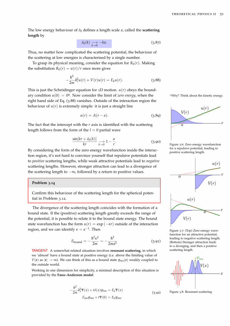
theoretical physics ii 51
The low energy behaviour of δ0 defines a length scale a, called the scatteringlength by
δ0(k) −→k→0−ka. (3.87)
Thus, no matter how complicated the scattering potential, the behaviour ofthe scattering at low energies is characterised by a single number.
To grasp its physical meaning, consider the equation for R0(r). Makingthe substitution R0(r) = u(r)/r once more gives
− h2
2m∂2
r u(r) + V(r)u(r) = Eku(r). (3.88)
This is just the Schrödinger equation for 1D motion. u(r) obeys the bound-ary condition u(0) = 04. Now consider the limit of zero energy, when the 4 Why? Think about the kinetic energy.
right hand side of Eq. (3.88) vanishes. Outside of the interaction region thebehaviour of u(r) is extremely simple: it is just a straight line
u(r) = A(r− a). (3.89)
The fact that the intercept with the r axis is identified with the scatteringlength follows from the form of the l = 0 partial wave
Figure 3.6: Zero energy wavefunctionfor a repulsive potential, leading topositive scattering length.
sin[kr + δ0(k)]kr
−→k→0
1− ar
. (3.90)
By considering the form of the zero energy wavefunction inside the interac-tion region, it’s not hard to convince yourself that repulsive potentials leadto positive scattering lengths, while weak attractive potentials lead to negativescattering lengths. However, stronger attraction can lead to a divergence ofthe scattering length to −∞, followed by a return to positive values.
Problem 3.14
Confirm this behaviour of the scattering length for the spherical poten-tial in Problem 3.12.
Figure 3.7: (Top) Zero energy wave-function for an attractive potential,leading to negative scattering length.(Bottom) Stronger attraction leadsto a diverging, and then a positivescattering length.
The divergence of the scattering length coincides with the formation of abound state. If the (positive) scattering length greatly exceeds the range ofthe potential, it is possible to relate it to the bound state energy. The boundstate wavefunction has the form u(r) = exp (−κr) outside of the interactionregion, and we can identify κ = a−1. Then
Ebound = − h2κ2
2m∼ − h2
2ma2 (3.91)
TANGENT A somewhat related situation involves resonant scattering, in whichwe ‘almost’ have a bound state at positive energy (i.e. above the limiting value ofV(r) as |r| → ∞). We can think of this as a bound state ψres(r) weakly coupled tothe outside world.
Working in one dimension for simplicity, a minimal description of this situation isprovided by the Fano–Anderson model
Figure 3.8: Resonant scattering− h2
2m∂2
xΨ(x) + tδ(x)ψres = EkΨ(x)
Eresψres + tΨ(0) = Ekψres.(3.92)

52 austen lamacraft
The odd solutions are unaffected by the resonant level, as they vanish at the origin.We write the even solutions as
Ψeven(x) = cos[k|x|+ δeven(k)] (3.93)
The first of Eq. (3.92) tells us that
sin δeven(k) =mth2 ψres. (3.94)
After solving the second for ψres we arrive at
tan δeven(k) =mh2
t2
Eres − Ek. (3.95)
The phase shift increases from 0 to π as we cross the resonance, taking the valueπ/2 when Ek = Eres.
Problem 3.15
Show that the reflection probability has the Breit–Wigner form
|r(k)|2 =γ2/4
(Ek − Eres)2 + γ2/4(3.96)
for some γ.
3.A Finding the Green’s function
We promised a more methodical derivation of the Green’s functionEq. (3.42). Starting from the defining equation Eq. (3.41)[
Ek +h2
2m∇2
]Gk(r, r′) = δ(r− r′), (3.41)
we find that the Fourier transform
Gk(r, r′) =∫ dq
(2π)3 Gk(q) exp(iq ·
[r− r′
])(3.97)
satisfies [k2 − q2
]Gk(q) =
2mh2 . (3.98)
The Green’s function is then given by the integral
Gk(r, r′) =2mh2
∫ dq(2π)3
exp (iq · [r− r′])k2 − q2
=m
π2h2|r− r′|
∫ ∞
0
sin q|r− r′|k2 − q2 q dq
=m
2π2ih2|r− r′|
∫ ∞
−∞
exp(iq|r− r′|)k2 − q2 q dq,
(3.99)
where in the second line we have done the angular integral, and in the thirdwe have extended the integral to whole of the real axis. This is done in orderto evaluate using the residue theorem. The integrand has poles at q = ±k,which lie on the integration contour. The residues at these poles areWe close the contour by adding a
semicircle ‘at infinity’ in the upper halfplane. Jordan’s lemma tells us that theintegral is unchanged. ∓1
2exp
(±ik|r− r′
)at q = ±k. (3.100)

theoretical physics ii 53
Notice that the residue at q = +k corresponds to an outgoing wave, whilethat at q = −k corresponds to an incoming wave. As in our treatment of theAiry function in Section 2.5, the physically relevant solution can be selectedby choosing the integration contour appropriately. In this case, the retardedGreen’s function is obtained by including only the pole at q = +k.
An alternative to deforming the contour is to add an infinitesimal quan-tity in the denominator
G+k (r, r′) =
m2πih2|r− r′|
∫ ∞
−∞
exp(iq|r− r′|)k2 − q2 + iε
q dq, (3.101)
which has the effect of pushing the pole at q = +k up a little bit, and that atq = −k down. Evaluating using the residue theorem gives Eq. (3.42).
Problem 3.16
Verify that Eq. (3.27), the Green’s function in 1D, is reproduced cor-rectly by this method.
Propagator and Green’s function
Now is a good opportunity to connect the Green’s function with the propa-gator of Chapter 2. Recall that the propagator is defined by[
ih∂
∂t− H
]K(r, t|r′, t′) = ihδ(r− r′)δ(t− t′) and
K(r, t|r′, t′) = 0 for t < t′.(2.8)
For a time independent Hamiltonian, we can represent the solution as aFourier integral over angular frequency as
K(r, t|r′, t′) =∫ ∞
−∞Kω(r|r′) exp
(−iω
[t− t′
]) dω
2π. (3.102)
The first part of Eq. (2.8) tells us that Kω(r|r′) satisfies
[hω− H]Kω(r|r′) = ihδ(r− r′). (3.103)
Comparison of Eq. (3.103) and Eq. (3.41) suggests that for H0 ≡ − h2
2m∇2
Kω(r|r′) ?= ihGk(r, r′) (3.104)
with h2k2
2m = hω. But what about the second part of Eq. (2.8)? For t < t′
we can, by Jordan’s lemma, close the contour of integration in Eq. (3.102) inthe upper half plane. If the integrand is analytic in this region, the integralvanishes, as required. From Eq. (3.101), we can see that the ‘+iε’ prescriptionthat we introduced to move the poles in the appropriate way also has theeffect of making G+
k (r, r′) analytic in the upper half plane of ω = hk2
2m , so thatthe Fourier integral over ω has the desired property. Thus we conclude
Kω(r|r′) = ihG+k (r, r′). (3.105)
This establishes the connection that we have been using all along betweenthe retarded nature of the propagator (in time) and the fact that G+
k (r, r′)contains only outgoing waves.

54 austen lamacraft
3.B Formal scattering theory
It is sometimes useful – if only to produce more compact expressions – towrite the Lippmann–Schwinger equation in a basis independent, operatorform:
|Ψk〉 = |ki〉+ G+k V |Ψk〉 , (3.106)
where |ki〉 is a plane wave state describing the incoming particle, and theoperator expression for the retarded Green’s function is
G+k = (Ek − H0 + iε)−1 . (3.107)
Here we have used the ‘+iε’ prescription discussed above. The nth orderterm in the Born series can then be written
〈kf|n times︷ ︸︸ ︷
G+k V · · ·G+
k V |ki〉 . (3.108)
Translating the formula Eq. (3.49) for the scattering amplitude givesUsing the normalization 〈r|k〉 =exp (ik · r) /(2π)3/2
f (kf, ki) = −√
2πmh2 〈kf|V|Ψk〉 . (3.109)
It’s convenient to define a transition operator T by
T |ki〉 = V |Ψk〉 . (3.110)
From Eq. (3.106), we see that T obeys the operator equation
T = V + VG+k T. (3.111)
The scattering amplitude is then given by the matrix elements of the transi-tion operator between initial and final plane wave states
f (kf, ki) = −4π2m
h2 〈kf|T|ki〉 . (3.112)
As an illustration of this formalism, consider the following computationNote that T is not Hermitian by virtueof the ‘+iε’ in the Green’s function.
〈Ψk|V|Ψk〉 = 〈Ψk|T|ki〉= 〈Ψk|V|ki〉+ 〈Ψk|VG+
k T|ki〉= 〈ki|T†|ki〉+ 〈ki|T†G+
k T|ki〉(3.113)
The left hand side is manifestly real.
Problem 3.17
By taking the imaginary part of the right hand side, show that thisyields (yet another) proof of the optical theorem. Hint: Use the formula
1x + iε
= P 1x− iπδ(x) (3.114)
where P denotes the principal value.

theoretical physics ii 55
3.C The quantum point contactThis discussion is based on (Glazmanet al., 1988).The quantum point contact (see Fig. 3.1) is a waveguide with width d(x)
varying with position x along the contact. Motion along the contact in thenth transverse mode can be described by the one dimensional Schrödingerequation.
Figure 3.9: Schematic view of a quan-tum point contact.
[− h2
2m∂2
x + En(x)
]Ψ(x) = EkΨ(x), (3.115)
where
En(x) =h2
2mπ2n2
d(x)2 (3.116)
is the transverse quantisation energy at x. Close to the centre of the contactwe can write
d(x) ∼ d0 +x2
R(3.117)
where R is the radius of curvature of the edge of the waveguide. In thisregion Eq. (3.115) takes the form[
−∂2x −
12
knx2]
Ψ(x) =
(k2 − π2n2
d20
)Ψ(x), (3.118)
where
kn =4π2n2
d30R
(3.119)
Eq. (3.118) is an inverted harmonic oscillator, and is soluble in terms ofparabolic cylinder functions. However, there is a way to understand what isgoing on without getting our hands too dirty. If the energy is large enough,we expect the WKB form of the wavefunction to be valid (see AQP)
ΨWKB(x) =A√p(x)
exp(
ih
∫ xp(x′)dx′
)+
B√p(x)
exp(− i
h
∫ xp(x′)dx′
).
(3.120)Now recall the trick we used to solve the Landau–Zener problem in Sec-tion 1.3. There we used a path in the plane of complex t, the time, on whichadiabaticity was not violated to solve a non-adiabatic problem. In exactlythe same way, we can use a path in complex x to solve a problem in whichthe WKB approximation breaks down for real x. In fact, it’s more or less thesame problem, as the functions ±p(x) that appear in the exponential areidentical to the E±(t) of Eq. (1.66).
The only difference is that the exponential factor analogous to Eq. (1.71)is now the ratio of the reflection to transmission coefficients, because oneoutgoing wave becomes the other as we pass around the branch point (c.f.Eq. (3.5))
RT
= exp
(−znπ2
√2Rd0
), zn =
kd0
π− n, (3.121)
where in the exponent we have made the simplification k2 − π2n2/d20 ∼
2πnd0
(k− πn/d0) for k ∼ πn/d0.

56 austen lamacraft
Problem 3.18
Verify this.
Using unitarity T + R = 1 we can therefore find the reflection coefficientexactly
R =1
1 + exp(
znπ2√
2Rd0
) . (3.122)
This shows that even for energies greater than the quantisation energy in themiddle of the waveguide there is overbarrier reflection, though the effectis small because of the numerical factors in the exponent. This explains thesharp conductance plateaux observed with relatively smooth constrictions(c.f. Fig. 3.1).

4Density matrices
There are known knowns; there are things we know that we know. There areknown unknowns; that is to say there are things that, we now know we don’tknow. But there are also unknown unknowns – there are things we do notknow we don’t know.
Donald Rumsfeld
The formalism of quantum mechanics that you have encountered up tonow is designed to deal with uncertainty. However, soon after the devel-opment of the modern form of the theory, it was realised that a tool wasneeded to describe a statistical distribution of quantum states. As we’ll see,such distributions arise in many situations, notably in quantum statisticalmechanics.
The appropriate concept, introduced independently in 1927 by von Neu-mann, Landau, and Bloch, is the density matrix (or operator). Before wedefine it, let’s see exactly why such a thing is necessary.
4.1 Two kinds of probability
Recall the Stern–Gerlach experiment of 1922 (AQP), in which a beam ofsilver atoms was split in two by a inhomogeneous magnetic field, on accountof the spin 1/2 of the outermost electron. Supposing that the atoms areindependent, how should we describe the beam?
Recall that the most general state of a spin 1/2 is
|n〉 =(
cos (θ/2) e−iφ/2
sin (θ/2) eiφ/2.
)(4.1)
This state has the property that it is an eigenstate of n · S with eigenvalue+h/2, where
n =
sin θ cos φ
sin θ sin φ
cos θ
. (4.2)
It’s clear that a single state of this form cannot describe the outermost elec-tron of each silver atom in the beam. If this were the case, orienting themagnetic field parallel to n would give a single, deflected beam, showingthat there was a preferred axis present.
We therefore need to describe the beam by an ensemble of quantum states,characterised by a probability distribution P(n). The expectation value ofany observable O can then be written as the integral over the unit sphere
〈O〉 =∫
dΩnP(n) 〈n|O|n〉 . (4.3)
58 austen lamacraft
The bar on the left hand side indicates we have taken an additional ensembleaverage, as well as the quantum average denoted by the angular brackets.We can rewrite this expression by introducing the operator
ρP ≡∫
dΩnP(n) |n〉 〈n| . (4.4)
Then we have〈O〉 = tr [ρPO] , (4.5)
where tr denotes the trace. The operator ρP is called the density matrix. Oneimmediate benefit of phrasing things in terms of ρP is that it makes it clearthat P(n) contains a great deal of redundancy. ρP is a 2× 2 Hermitian matrix
ρ†P = ρP, (4.6a)
and therefore depends on only 4 real parameters, rather than a continuousfunction. In fact, there is are two more conditions. By taking O = 1 inEq. (4.5)
tr ρP = 1. (4.6b)
Thus there are only three real parameters. Finally, it is clear from the defini-tion Eq. (4.4) and the positivity of the probability distribution that
〈Ψ|ρP|Ψ〉 ≥ 0 (4.6c)
for all |Ψ〉. We say that ρP is positive semi definite.At this point let’s dispense with P(n) altogether, and define a density
matrix to be any operator satisfying the three conditions Eqs. (4.6). Theexpectation value of any observable is given by Eq. (4.5)
Problem 4.1
Show that the most general form of a spin 1/2 density matrix is
ρ =121+
r2
n · σ (4.7)
for 0 ≤ r ≤ 1. Thus, the space of spin 1/2 density matrices is identifiedwith the unit ball (Bloch sphere).
The density matrix reflects our ignorance of the quantum state of the system.A system described by a general density matrix is said to be in a mixedstate.
Since ρ is Hermitian, it has a representation in terms of its eigenvaluesand (orthogonal) eigenstates
ρ = ∑α
Pα |ϕα〉 〈ϕα| . (4.8)
The conditions Eq. (4.6b) and Eq. (4.6c) imply
∑α
Pα = 1 and Pα ≥ 0. (4.9)
Thus, although the definition provided by Eqs. (4.6) looked abstract, wesee that it is equivalent to specifying a probability distribution Pα on anorthogonal basis of states |ϕα〉, which could be discrete or continuous. Theexpectation value Eq. (4.5) takes the form
〈O〉 = ∑α
Pα 〈ϕα|O|ϕα〉 (4.10)

theoretical physics ii 59
Problem 4.2
What is the density matrix appropriate for spins in the Stern–Gerlachexperiment?
A pure state corresponds to having one of the Pα = 1, in which caseρ = |ϕα〉 〈ϕα|, a projector on the corresponding state.
We’ll return to the Stern–Gerlach experiment shortly, after we have dis-cussed the density matrix in the position representation.
TANGENT Although we won’t pursue it further, the representation of the den-sity matrix given by Eq. (4.4) is often used in quantum optics and is called the Prepresentation. For modes of the light field |n〉 is replaced by a coherent state |α〉(see AQP), and integration over the plane of complex α replaces integration overthe unit sphere. In this context, the P representation is known as the Sudarshan–Glauber representation (for which Glauber was awarded the Nobel prize in 2005 –you may very well wonder what happened to Sudarshan).
Very roughly, the idea of this representation is to describe the quantum state interms of a distribution function of a classical quantity, such as an amplitude α
or spin direction n. However, this viewpoint is subject to various complications.One drawback of the P representation is that it is not positive. That is, a non-negative ρP can correspond to a P that is not everywhere positive. An alternativerepresentation is the Husimi or Q representation
Q(α) =1π〈α|ρ|α〉 , (4.11)
which is manifestly positive. For more on the applications of these ideas in quan-tum optics, see (Scully and Zubairy, 1997). The bible of coherent states is (Perelo-mov, 1986).
The position representation
The density matrix is simple enough for the two dimensional space of spin1/2, but in general we need to work with infinite dimensional spaces. Bar-ring any mathematical mishaps, the defining conditions Eqs. (4.6) carry overto the general case. We can then form the position representation of the den-sity matrix by taking matrix elements in the usual way
ρ(r, r′) = 〈r|ρ|r′〉 . (4.12)
In terms of the matrix elements of an observable O(r, r′) = 〈r|O|r′〉, theexpectation value may be written
〈O〉 = tr [ρO] =∫
dr dr′ ρ(r, r′)O(r′, r) (4.13)
Problem 4.3
Show that the expectation value of the momentum is
〈p〉 = ih∫
dr∇rρ(r, r′)∣∣∣r′=r
. (4.14)
In terms of the eigenvalues and eigenstates of the density matrix we have
ρ(r, r′) = ∑α
Pα ϕα(r)ϕ∗α(r′) (4.15)

60 austen lamacraft
where ϕα(r) = 〈r|ϕα〉. The diagonal element of the density matrix
ρ(r, r) = ∑α
Pα|ϕα(r)|2, (4.16)
gives the probability of finding the particle at position r. This is a generalfeature of the diagonal matrix elements in any orthogonal basis.
4.2 Time evolution of the density matrix
The equation of motion of the density matrix is easy to obtain from the timedependent Schrödinger equation describing the evolution of an arbitrarystate
ihddt|Ψ〉 = H |Ψ〉 . (4.17)
Applied to the spectral representation Eq. (4.8), this immediately gives thevon Neumann equationNote the sign difference between
the von Neumann equation andHeisenberg’s equation of motiondOdt = i
h [H,O]. In the present case westay within the Schrödinger picture i.e.the states are evolving, rather than theobervables.
dρ
dt= − i
h[H, ρ] . (4.18)
The formal solution of this equation is
ρ(t) = U(t, t′)ρ(t′)U†(t, t′), (4.19)
where U(t, t′) is the unitary operator of time evolution. This evolution pre-serves the eigenvalues Pα of the density matrix.
Problem 4.4
Describe the evolution of the spin 1/2 density matrix of Problem 4.1when H = H · S.
With the equation of motion in hand we can return to the Stern–Gerlachexperiment. The wavefunction of our spin 1/2 particles consists of a spincomponent and a spatial part (the internal structure of the atoms can beignored, in the spirit of the adiabatic approximation), so our density matrixhas the general form (
ρ↑↑(r, r′) ρ↑↓(r, r′)ρ↓↑(r, r′) ρ↓↓(r, r′).
)(4.20)
We suppose that the magnetic field varies only in a direction transverse tothe beam direction, so the longitudinal motion of the particles factors out ofthe problem. The Hamiltonian can then be taken to be
H = − h2
2m∂2
x − µB′xσz, (4.21)
where B′ is the magnetic field gradient and µ is the magnetic moment. LetΨ0(x, t) be the wavefunction of a particle in the absence of a field gradient.In this case the density matrix would evolve as
ρ(x, x′; t = 0) =
(1/2 0
0 1/2
)Ψ0(x, t)Ψ∗0(x′, t). (4.22)
The Hamiltonian Eq. (4.21) is diagonal in the spin, so we just need to findhow the wavepackets of an up spin and down spin particle evolve in the

theoretical physics ii 61
presence of the field gradient. Because the gradient is constant, this turnsout to be very simple
Ψ↑,↓(x, t) = exp(iθ↑,↓(x, t)/h
)Ψ0(x∓ µB′t2/2m, t), (4.23)
where the phase θ↑,↓(x, t) is
θ↑,↓(x, t) = ±µB′xt− (µB′)2t3
6m(4.24)
Problem 4.5
Prove this.
Notice that – apart from the phase factor – the effect of the gradient is toshift the wavepacket to the point ±µB′t2/2m, which corresponds to theclassical trajectory of a particle in a linear potential.
The evolution of the density matrix is then
ρ(x, x′; t) =12
(Ψ↑(x, t)Ψ∗↑(x′, t) 0
0 Ψ↓(x, t)Ψ∗↓(x′, t)
). (4.25)
The diagonal elements take on a particularly simple form
ρ↑↑(x, x; t) =12|Ψ0(x− µB′t2/2m, t)|2
ρ↓↓(x, x; t) =12|Ψ0(x + µB′t2/2m, t)|2.
(4.26)
Remembering that the diagonal elements of the density matrix give theprobability to be in a particular location with a particular spin component,we see that this describes the splitting of the beam into two.
Comparing Eq. (4.22) and Eq. (4.25), we see that in the first case the spinand position degrees of freedom of the particles are independent of eachother – the density matrix factorizes – while in the second case they areentangled1. 1 This term was introduced by
Schrödinger, who called it ‘the charac-teristic trait of quantum mechanics’.TANGENT The von Neumann equation is the quantum counterpart of Liouville’s
equation of classical mechanics
∂ρ
∂t= −ρ, HP , (4.27)
where ρ(q, p, t) is the phase space density and ·, · denotes the Poisson bracket
f , gP =∂ f∂q· ∂g
∂p− ∂ f
∂p· ∂g
∂q. (4.28)
Eq. (4.27) can be written as a continutity equation Note the appearance of a partialderivative on the left hand side ofLiouville’s equation compared to atotal derivative in von Neumann’sequation. This is just because ρ in aclassical mechanics is a function onphase space. We mention this becauseLiouville’s equation is sometimeswritten as dρ
dt = 0, which includes thevariation due to the time dependenceof (q(t), p(t)), evolving according toHamilton’s equations.
∂ρ
∂t+ ∂i (viρ) = 0, (4.29)
and describes a flow in phase space due to the Hamiltonian vector field
vi =
∂H∂pi
i = 1, . . . , N
− ∂H∂qi−N
i = N + 1, . . . , 2N,(4.30)
where the first N coordinates are the positions and the second N are the momenta.Note that in writing Eq. (4.29) we used the fact that the flow is incompressible(∂ivi = 0), which is the content of Liouville’s theorem.

62 austen lamacraft
The resemblance between Eq. (4.27) and Eq. (4.18) is an example of the moregeneral correspondence
A, B ←→ − ih[A, B] , (4.31)
between Poisson brackets in classical mechanics and commutators of operators inquantum theory.
Of course, this relationship is purely formal, as functions on phase space and oper-ators in Hilbert space are very different things. A closer link may be established byconsidering the Wigner function
$(q, p) =∫
dr ρ(q + r/2, q− r/2) exp(− i
hp · r
)(4.32)
obtained by Fourier transforming with respect to the difference of the arguments ofthe density matrix. $(q, p) is the quantum mechanical analog of the classical phasespace density, though in general it is not positive. The von Neumann equationimplies the equation of motion for $(q, p)
∂$
∂t= −$, HM , (4.33)
where ·, ·M denotes the Moyal bracket
f , gM =2h
f (q, p) sin(
h2
[←−∂q ·−→∂p −
←−∂p ·−→∂q
])g(q, p). (4.34)
If we retain only the leading order term in h, corresponding to the classical limit,we recover Liouville’s equation.
Problem 4.6
Use Eq. (4.33) to explain why the linear potential in Eq. (4.21) has such asimple effect on the evolution of the density matrix.
4.3 The density matrix in statistical mechanics
Perhaps the most important mixed state that we encounter is that describingthermal equilibrium. Just as our ignorance of the microstate of a systemis described in classical statistical mechanics by a probability distributionρ(q, p) in phase space, so our ignorance of the quantum microstate of asystem corresponds to a density matrix.
There are a number of variants, according to the ensemble we work with.
• In the microcanonical ensemble, corresponding to fixed energy E andnumber of particles, the density matrix takes the form
ρm =1
N(E, δE) ∑α∈A(E,δE)
|ϕα〉 〈ϕα| , (4.35)
where the set A(E, δE) includes all energy eigenstates in the range(E− δE, E + δE), and N(E, δE) is the number of such states, which isneeded to correctly normalize the density matrix. δE is a microscopicallylarge but macroscopically small energy interval, meaning that it contains alarge number of states but δE/E 1.
• In the canonical ensemble, with fixed temperature T and number ofparticles, we have
ρc =1Z
exp (−βH) , (4.36)

theoretical physics ii 63
where β = 1/(kBT), and kB is Boltzmann’s constant. The normalizationfactor that guarantees the trace of the density matrix is unity is called thepartition function
Z = tr [exp (−βH)] . (4.37)
Finally, in the grand canonical ensemble, with fixed temperature andchemical potential µ, we have
ρgc =1Z exp (−β [H − µN]) . (4.38)
The grand canonical partition function is defined just as in Eq. (4.37). Thedifference from the canonical case is that the Hilbert space is now takento be the Fock space of many particle states, and includes states withdiffering numbers of particles. More on this in Chapter 5.
Note that all of these density matrices, being functions of the Hamiltonian(and number of particles in the grand canonical case), are constant in time.
The partition function and density matrix appear in a great many thermo-dynamic relationships, of which we list expressions for the average energy,Helmholtz free energy F, and entropy S
E = 〈H〉 = − ∂
∂βln Z
F = −kBT ln Z
S = −k tr (ρ ln ρ) = −k ∑α
Pα ln Pα.
(4.39)
The above expression for the entropy is called the von Neumann entropy(the corresponding expression in classical statistical mechanics is called theGibbs entropy). The same expression appears in
information theory, where it quantifiesthe information content of a messageand is known as Shannon entropy,after Claude Shannon. It was vonNeumann who suggested the name toShannon, saying: ‘You should call itentropy, for two reasons. In the firstplace your uncertainty function hasbeen used in statistical mechanicsunder that name, so it already has aname. In the second place, and moreimportant, no one really knows whatentropy really is, so in a debate youwill always have the advantage.’.
Problem 4.7
Show that the von Neumann entropy follows from the first two expres-sions in Eq. (4.39) and the definition F = E − TS of the Helmholtz freeenergy.
Note that the von Neumann entropy does not coincide with the thermo-dynamic entropy of an isolated system out of equilibrium, because it doesnot change in time.
Problem 4.8
Prove this.
However, the von Neumann entropy is useful for other things. In particu-lar, it measures the departure from a pure state, where it vanishes.
The canonical density matrix
As you will be aware, most calculations in statistical mechanics are moreeasily done at fixed temperature than fixed energy, making the canonicalensemble preferred over the microcanonical ensemble.

64 austen lamacraft
In quantum statistical mechanics, there is another reason to favour thecanonical ensemble. ρc closely resembles the time evolution operator
U(t) = exp (−iHt/h) , (4.40)
except that we ‘evolve’ for an imaginary time t = −ihβ. The wonderfulthing about this observation is that all of the techniques that are available tocompute the time evolution of a quantum state can immediately be appliedto calculate the density matrix.
The evolution is of course not unitary, but this is more of a blessing thana curse as the usual result is to improve convergence in numerical work: thedensity matrix is real, indeed positive, rather than complex and oscillating.
From our calculation of the free particle propagator Eq. (2.13) , we canimmediately write down
〈r| exp (−βH) |r′〉 =(
m2πh2β
)3/2
exp
[−m(r− r′)2
2h2β
]. (4.41)
Calculating the normalization for a particle in a box of volume V gives thepartition function
Z =V
λ3dB
(4.42)
where λdB is the thermal de Broglie wavelength
λdB ≡
√2πβh2
m. (4.43)
Thus we obtain the density matrix
ρfree(r, r′) =1V
exp
(−π|r− r′|2
λ2dB
). (4.44)
which nicely captures the intuition that at finite temperature a particle has atypical wavelength λdB.
Quantum degeneracy corrections to the ideal gas law
To see the density matrix in action, let’s compute the partition function ofa gas of indistinguishable non interacting particles. To take into accountindistinguishability, we must work with totally symmetric or antisymmet-ric wavefunctions depending on whether we are dealing with bosons orfermions (see Chapter 5 of these notes). This means that we take matrixelements of the density matrix between the states
|r1, . . . , rN〉S/A =1√N!
∑P
ηS/A(P) |rP1, . . . , rPN〉 . (4.45)
The sum is over all N! permutations P of N objects. We have introducedηS/A in order to write the following expressions in a unified way for bosons(S) and fermions (A). Thus ηS(P) = 1 and ηA(P) = sgn(P), the signature ofthe permutation2.2 The signature of a permutation is
equal to +1 for permutations involv-ing an even number of exchanges, and−1 for an odd number.
In this way we find the expression for the N particle partition function
ZN =1
N!λ3NdB
∑P
∫dr1 · · · drN ηS/A(P) exp
(− π
λ2dB
N
∑j=1|rj − rPj|2
). (4.46)

theoretical physics ii 65
This is a rather fearsome looking expression, but it has a simple meaning:when taking the trace of exp (−βH) we have to account for the fact thatthe diagonal elements of the density matrix are those where the two sets ofparticle position labels differ by a permutation.
Of course, evaluating it is another matter! We can, however, makeprogress in the limit of high temperatures, where the de Broglie wavelengthis short. Then the non trivial permutations in Eq. (4.46) hardly contribute,because some of the Gaussian factors that appear will be small.
Retaining only the identity permutation, we get
ZN ∼1
N!
(V
λ3dB
)N
. (4.47)
Eq. (4.39) and p = − ∂F∂V
∣∣T for the pressure then give the ideal gas law pV =
NkBT.We can do a bit better than this without too much effort, by taking into
account those permutations that involve only a single transposition, as thesewill evidently be the next largest.
Problem 4.9
Show that this yields the correction to the ideal gas law
pV = NkBT
[1∓ λ3
dBn25/2 + · · ·
], (4.48)
with the minus sign for boson and the plus sign for fermions. n = NV is
the density.
Coming from high temperatures, where nλ3dB 1, this is the first indica-
tion of a difference in the thermodynamic behaviour of ideal Bose and Fermigases. Of course, you know that when nλ3
dB ∼ 1 this difference is very pro-nounced, with the possibility of Bose–Einstein condensation in the case ofbosons.
It’s interesting to ask how condensation appears in this framework. Anypermutation can decomposed into set of cycles. For example, the permuta-tion (1, 2, 3, 4) → (4, 2, 1, 3) can be written as the cycle 1 → 4 → 3 → 1and the trivial cycle 2 → 2. In deriving Eq. (4.48) we just took into account1-cycles and 2-cycles.
(Feynman, 1953) conjectured that condensation is associated with theappearance of a finite density of infinite cycles in the thermodynamic limit, anidea that was later established rigorously.
TANGENT Of course, for noninteracting particles, the above calculation is mosteasily handled within the grand canonical framework. The canonical picturereally comes into its own as a numerical tool called the path integral Monte Carlomethod. The idea is to represent the partition function of an interacting systemjust as in Eq. (4.46), but with the corresponding propagator taking the place ofthe free propagator. Because we are working in imaginary time, the integrand forbosons is a positive quantity that can be interpreted as a probability distributionon the space of paths and sampled accordingly. This method has been successfullyapplied to the study of superfluid Helium, Feynman’s original concern in the workmentioned above.
Figure 1. Cartoon of a path for 3 particles (A, B, C) with M = 4, ! = "/4. The kinetic terms are representedby zig-zag lines and potential by dotted lines. Note that dotted lines connect only beads of the polymers at thesame time
Figure 2. The trace of the close paths of six helium atoms at a temperature of 2K with M = 80. Straightlines (kinetic term) connect successive beads of the polymers. The filled circles are markers for the (arbitrary)beginning of the path. The paths have been replicated using the periodic conditions. The dashed lines representthe simulation cell.
2.3 Definition of the Action
The action is defined as minus the logarithm of the density matrix. For a given link m (seeEq. 13), one has:
Sm ! S(Rm!1, Rm; !) ! " ln["(Rm!1, Rm; !)]. (23)
55
Figure 4.1: Path integral Monte Carlotrajectories of six Helium atoms(periodic boundary conditions). From(Bernu and Ceperley, 2008).

66 austen lamacraft
Unfortunately, the minus sign in the case of fermions stymies the straightforwardapplication of this method, a situation generally known as the fermion sign prob-lem.
4.4 Density operator for subsystems and quantum entanglement
We introduced density matrices to describe a situation where the quantumstate of a system is not definite, but drawn from a probability distribution.We didn’t address the question of how such a situation arises in the firstplace. Of course, the density matrix could just represent the incompletenessof our knowledge of the quantum state. Here, we discuss another naturalway in which the density matrix appears when we consider a subsystem ofa larger quantum system, itself described by a pure state. We will encounteragain the notion of entanglement, which we met briefly in Section 4.2. In thissection we are going to explore this a little more deeply, using a pair of spinsas our main example.
Two spins 1/2 are described by a four dimensional Hilbert space, spannedby the following basis of statesThis mathematical term for making a
larger space out of two smaller spacesin this way is tensor product. It’s nothard to see that the dimension of theresulting space is the product of thedimensions of the constituent spaces.
|A〉 = |↑〉1 |↑〉2 , |B〉 = |↑〉1 |↓〉2|C〉 = |↓〉1 |↑〉2 , |D〉 = |↓〉1 |↓〉2 .
(4.49)
Here |↑〉 and |↓〉 are eigenstates of σz with eigenvalue ±1, and the labels 1and 2 are just to emphasize that we are dealing with the first or second spin(although the position also tells us which).
A pure state of the two spin system is described by the density matrix
ρ2 spin = |φ〉 〈φ| (4.50)
where |φ〉 is some linear combination of the states in Eq. (4.49).
|φ〉 = α |A〉+ β |B〉+ γ |C〉+ δ |D〉 (4.51)
Note that ρ2 spin is a 4× 4 matrix. Its explicit form in the above basis is
ρ2 spin =
|α|2 αβ∗ αγ∗ αδ∗
βα∗ |β|2 βγ∗ βδ∗
γα∗ γβ∗ |γ|2 γδ∗
δα∗ δβ∗ δγ∗ |δ|2.
(4.52)
As we know, any expectation value can be computed by multiplying thecorresponding operator by the density matrix and taking the trace
〈O〉 = tr[ρ2 spinO
]= 〈φ|O|φ〉 , (4.53)
which in this case is just the pure state expectation value. Now, suppose thatthe operator O lives in the Hilbert space of the first spin, e.g. O1 = σi,1. Theexpectation value is then
〈O1〉 =(|α|2 + |β|2
)〈↑ |O| ↑〉+
(|γ|2 + |δ|2
)〈↓ |O| ↓〉
(α∗γ + β∗δ) 〈↑ |O| ↓〉+ (αγ∗ + βδ∗) 〈↓ |O| ↑〉≡ tr[ρ1reducedO]
(4.54)

theoretical physics ii 67
where in the last line we have defined the reduced density matrix
ρ1 red =
(|α|2 + |β|2 αγ∗ + βδ∗
α∗γ + β∗δ |γ|2 + |δ|2,
)(4.55)
in the |↑, ↓〉1 basis of spin 1.In general ρ1 red describes a mixed state of spin 1. More generally, we can
writeρ1 red = tr
2[ρ2 spin] (4.56)
where tr2 [· · · ] denotes the trace over the space of spin 2. To get a feel forwhat this means, compare Eq. (4.52) and Eq. (4.55).
The reduced density matrix contains all the information we need aboutthe system if we only ask questions (= make measurements) on spin 1.
Problem 4.10
What about the converse problem? That is, for any density matrix of asingle spin, is is possible to view it as the reduced density matrix of apure state of two spins? If so, is the pure state unique? This process iscalled purification of a density matrix.
The reduced density matrix can be treated like any other density matrix.Its lack of purity is a reflection of the entanglement between the two systemsthat prevents us describing the subsystem by a pure quantum state. We sawthat the von Neumann entropy of a density matrix can be used to measurethe departure from a pure state. Therefore the quantity
Sent ≡ − tr [ρred log ρred] , (4.57)
measures the degree of entanglement between two subsystems, and isknown as the entanglement entropy.


5Second quantization
Each photon then interferes only with itself. Interference between two differentphotons never occurs.
Dirac, Principles of Quantum MechanicsDirac was wrong about this, as we’llsee in this chapter.A system of N particles is described by a wavefunction of N position
arguments Ψ(r1, r2, . . . , rN). For indistinguishable particles, you will havealready met the idea that the wavefunction should be taken to be totallysymmetric or totally antisymmetric under exchange of any pair of particles(see AQP). We’ll review this idea and its consequences in the next section.
The wavefunction language is not a convenient one, however, when wecome to discuss the quantum mechanics of a truly macroscopic numberof particles. Only in certain special cases can a compact expression for thewavefunction be obtained for an arbitrary number of particles (we’ll meetsuch an example shortly). Even then, evaluating observables typically in-volves integrals over every particle coordinate: an arduous task. Fortunately,there is a formalism that is well suited to the general case, in which indis-tinguishability is built in from the outset rather than imposed upon thewavefunction. This formalism is called second quantization. The name is very obscure, but will
become a bit clearer later.
5.1 Quantum indistinguishability: bosons and fermions
A pair of particles is described by a wavefunction Ψ(y, x). If the particlesare indistinguishable, the associated probability density must be unchangedupon exchange of the positions of any pair1 1 This is what we mean by indistin-
guishable.|Ψ(y, x)|2 = |Ψ(x, y)|2. (5.1)
More precisely, Ψ(x, y) and Ψ(y, x) must correspond to the same quantumstate, meaning that they can differ only by a (constant) phase
Ψ(y, x) = eiθΨ(x, y).
What can we say about θ? Take another two positions x′, and y′, then
Ψ(y′, x′) = eiθΨ(x′, y′),
but there’s nothing to stop us taking x = y′, and y = x′, in which case wecan combine these two expressions to give
Ψ(x, y) = e2iθΨ(x, y) (5.2)
that is eiθ = ±1 and the wavefunction for two particles is either symmetric orantisymmetric.

70 austen lamacraft
A more formal approach is to consider the exchange operator P12 thatexchanges the two arguments
P12Ψ(x, y) = Ψ(y, x)
which is evidently a linear operator that furthermore squares to give theidentity P2
12 = 1. The eigenvalues of P12 are therefore ±1, with the corre-sponding eigenstates being symmetric or antisymmetric respectively.
The exchange operator commutes with the Hamiltonian of a pair of iden-tical particles. As an example, consider the Hamiltonian for a pair of elec-trons
H = − h2
2me
[∇2
x +∇2y
]+
e2
|x− y| (5.3)
evidently it doesn’t matter whether we apply P12 before or after H. Thus[H, P12] = 0 and basic ideas of quantum mechanics tell us that
1. Eigenstates of the Hamiltonian have definite exchange symmetry2.2 In a real two-electron system overallantisymmetry is guaranteed by the ap-propriate choice of spin wavefunction. 2. The symmetry of the wavefunction is a constant of the motion.
From two to many
What changes when we consider systems of N identical particles? The wave-function is now a function of the N coordinates Ψ(r1, r2, . . . , rN), and we canconsider an exchange operator Pij that swaps the ith and jth arguments. Thesame physical reasoning as before singles out eigenstates of the Pij. Notethat [P12, P23] 6= 0, and thus one might worry whether it is mathematicallypossible to have a simultaneous eigenstate of all the Pij. We see straightawaythat a totally symmetric state with all eigenvalues equal to +1 is allowed.What about a totally antisymmetric state with all eigenvalues −1? This too ispossible for the following reason. Any given permutation may be writtenin many different ways as a product of exchanges (see the next problem foran example). For a given permutation, however, these different possibilitieseither involve only even numbers of exchanges, or only odd numbers, a factwe’ll prove below.
Problem 5.1
By showing that P12P23P12 = P13 = P23P12P23 prove that a simultaneouseigenstate of all the Pij must have all eigenvalues +1 or all −1, that is,be totally symmetric or totally antisymmetric.
All of this shows that any given species of quantum particle will fallinto one of two fundamental classes: symmetric bosons and antisymmetricfermions, named for Bose and Fermi respectively (the whimsical terminol-ogy is Dirac’s). The distinction works equally well for composite particles,provide we ignore the internal degrees of freedom and discuss only the cen-ter of mass coordinate. All matter in the universe is made up of fermions:Easy for us to say. Here’s Dirac again:
‘The solution with antisymmetricaleigenfunctions, though, is probablythe correct one for gas molecules, sinceit is known to be the correct one forelectrons in an atom, and one wouldexpect molecules to resemble electronsmore closely than light-quanta.’ (Dirac,1926)
electrons, quarks, etc., but you can easily convince yourself that an evennumber of fermions make a composite boson (e.g. a 4He atom with two elec-trons, two neutrons and two protons) and an odd number make a compositefermion (3He has one fewer neutron, which in turn is made up of 3 quarks).

theoretical physics ii 71
If we dealt with distinguishable particles, the wavefunction of a pair ofparticles in states ϕ1 and ϕ2 would be
Ψ(r1, r2) = ϕ1(r1)ϕ2(r2). (5.4)
Accounting for indistinguishability, we have either The 1/√
2 yields a normalized wave-function if ϕ1,2(r) are orthonormal.
Ψ(r1, r2) =1√2[ϕ1(r1)ϕ2(r2)± ϕ2(r1)ϕ1(r2)] (5.5)
with the upper sign for bosons and the lower for fermions. Note in particu-lar that when ϕ1 = ϕ2 the fermion wavefunction vanishes. This illustrates thePauli exclusion principle, that no two identical fermions can be in the samequantum state. There is no such restriction for bosons.
Problem 5.2
Classically, if you had a function P1(r1) describing the probability den-sity of finding particle 1 at position r1, and the corresponding quantityfor an independent particle 2, you would have no hesitation in conclud-ing that the joint distribution is
P12(r1, r2) = P1(r1)P2(r2). (5.6)
This also follows from taking the square modulus of Eq. (5.4). What isthe result implied by the wavefunction Eq. (5.5) for a pair of identicalbosons or fermions?
Most people find this result rather counterintuitive. It shows that, becauseprobabilities arise from the squares of amplitudes, identical particles inquantum mechanics are never truly independent.
Figure 5.1: Four possible outcomes af-ter the passage of two bosons througha beam splitter.
Problem 5.3
One dramatic illustration of this deviation from our classical intuition isprovided by the Hong–Ou–Mandel effect in quantum optics (Fig. 5.1).In simplified terms, we imagine wavepackets describing two bosonsapproaching a 50:50 beam splitter from either side. Because of the uni-tarity of scattering, the two bosons end up in orthogonal states. Forexample,
1√2(|Left〉 ± |Right〉) . (5.7)
Apply the result of the previous problem to deduce the probabilities ofthe four possible outcomes.

72 austen lamacraft
The Hamiltonian of a system of N identical noninteracting particles isa sum of N identical single particle Hamiltonians, that is, with each termacting on a different particle coordinate
H =N
∑i=1
[− h2
2m∇2
i + V(ri)
](5.8)
where m is the particle mass, and V(ri) is a potential experienced by theparticles. Let’s denote the eigenstates of the single particle Hamiltonian byϕα(r), and the corresponding eigenenergies by Eα, where α is a short-hand for whatever quantum numbers are used to label the states. A set of la-bels αi i = 1, 2, . . . N tells us the state of each of the particles. Thus we canwrite an eigenstate of N distinguishable particles with energy E = ∑N
i=1 Eαi as33 We will frequently switch betweenthe wavefunction (ϕ(x)) and bra-ketnotation (|ϕ〉). In the latter notation theproduct wavefunction in Eq. (5.4) iswritten |ϕ1〉 |ϕ2〉. |Ψα1α2···αN 〉 = ϕα1(r1)ϕα2(r1) · · · ϕαN (r1). (5.9)
A general state will be expressed as a superposition of such states, of course.As we’ve just discussed, however, we should really be dealing with a totallysymmetric or totally antisymmetric wavefunction, depending on whetherour identical particles are bosons or fermions. To write these down we intro-duce the operators of symmetrization and antisymmetrization
S =1
N! ∑P
P, A =1
N! ∑P
sgn(P)P. (5.10)
The sums are over all N! permutations of N objects, P denotes the corre-sponding permutation operator, and sgn(P) is the signature of the permuta-tion, equal to +1 for permutations involving an even number of exchanges,and −1 for an odd number. This allows us to write the totally symmetricand totally antisymmetric versions of Eq. (5.9) as
ΨSα1α2···αN
(r1, . . . , rN =
√N!
∏α Nα!S ϕα1(r1)ϕα2(r2) · · · ϕαN (rN)∣∣∣ΨA
α1α2···αN
⟩=√
N!A ϕα1(r1)ϕα2(r2) · · · ϕαN (rN) (5.11)
Such states are called product states. The normalization factor in the bosonThe normalization factors yield nor-malized wavefunctions if the singleparticle state |ϕα〉 are orthonormal (asthe eigenstates of the single particleHamiltonian are).
case involves the occupation numbers Nα giving the number of particlesin state α. In the fermion case each Nα is either 0 or 1 so the prefactor sim-plifies. Since the order of the α indices is irrelevant in the boson case, andamounts only to a sign in the fermion case, states based on a given set ofsingle particle states are more efficiently labeled by the occupation numbers.In terms of these numbers the total energy is
E =N
∑i=1
Eαi = ∑α
NαEα (5.12)

theoretical physics ii 73
Problem 5.4
Find
1. The totally antisymmetric state of three fermions in states ϕ1, ϕ2,and ϕ3
2. The totally symmetric state of three bosons, with two in state ϕ1 andone in state ϕ2.
Problem 5.5
Verify that the normalization factors in Eq. (5.11) are correct.
A more formal way of putting things is as follows. We first consider thespace spanned by states of the form Eq. (5.9). Then we introduce the oper-ators S and A, noting that S2 = S and A2 = A. In other words, there’sno point symmetrizing or antisymmetrizing more than once (we say thatthe operators are idempotent). Any eigenvalue of one of these operators istherefore either one or zero. The states with S = 1 are the symmetric states,and those with A = 1 are antisymmetric. You can easily convince yourselfthat if a state has one of S or A equal to one, the other is zero. This definessymmetric and antisymmetric subspaces, consisting of the admissible bosonand fermion wavefunctions.
Note that the fermion wavefunction takes the form of a determinant (usu-ally called a Slater determinant4) 4 Though it appears first in (Dirac,
1926).
∣∣∣ΨAα1α2···αN
⟩=
1√N!
∣∣∣∣∣∣∣∣∣ϕα1(r1) ϕα1(r2) · · · ϕα1(rN)
ϕα2(r1) · · · · · · · · ·· · · · · · · · · · · ·
ϕαN (r1) · · · · · · ϕαN (rN)
∣∣∣∣∣∣∣∣∣ . (5.13)
The vanishing of a determinant when two rows or two columns are identicalmeans that the wavefunction is zero if two particle coordinates coincide(ri = rj), or if two particles occupy the same state (αi = αj).
TANGENT We pause here to note that the above arguments – which appear inmost textbooks in one variant or another – suffer from a deficiency that remainedundiscovered until (Leinaas and Myrheim, 1977). The weak point is that nothingrequires that the wavefunction of a pair be single-valued, as we tacitly assumed inwriting Eq. (5.2). Compare this situation with our dis-
cussion of Berry’s phase in Section 1.4.In that case the phase accumulateddoes depend on the path, becausethe associated vector potential has anon-zero ‘magnetic field’. This has adynamical effect even for a classicalparticle. The present discussion ismore closely related to the Aharonov–Bohm, which you met briefly in AQP,where the particle moves in a region ofzero magnetic field.
Let’s examine the argument a little more closely. Imagine our pair of particlesremain always at the same distance from each other, and only relative motion isimportant. In terms of the unit vector n = (x− y) /|x− y|, an exchange then corre-sponds to n → −n i.e. tracing a path on the unit sphere that starts and finishes atantipodal points. A double exchange corresponds to a complete circumnavigation.We associate a phase factor e2iθ with this path. Assuming that this phase is inde-pendent of the path, we can now consider contracting this path to nothing, whichshows that our original conclusion that e2iθ = 1 is solid.
The situation changes drastically if we consider particles confined to two spatialdimensions. Then our double exchange corresponds to going once around a circle.Such a path cannot be deformed smoothly to nothing, and as a result e2iθ canin principle be anything at all. Particles whose statistics lie in this continuum ofpossibilities between bosons and fermions in two dimensions were dubbed anyonsby Frank Wilczek (Wilczek, 1982).

74 austen lamacraft
Of course, our world is three dimensional, which seems to make this possibility oflimited interest. Even if we happen to confine particles to two dimensions, the factthat they can really move in three means that the original argument applies. Thisreasoning does not hold, however, for collective excitations of a many body systemconfined to two dimensions. Remarkably, anyonic excitations do in fact occur inthe fractional quantum Hall effect, a phenomenon observed in two dimensionalelectron systems in high magnetic fields.
5.2 Example: particles on a ring
Let’s consider perhaps the simplest many particle system one can think of:non-interacting particles on a ring. If the ring has circumference L, the singleparticle eigenstates are
ϕn(x) =1√L
exp(
2πinxL
), n = 0,±1,±2, . . . (5.14)
with energies En = h2n2
2mL2 . Let’s find the N particle ground state. For bosonsevery particle is in the state ϕ0 with zero energy: N0 = N. Thus (ignoringnormalization)
ΨS(x1, x2, . . . xN) = 1.
That was easy! The fermion case is harder. Since the occupation of eachlevel is at most one, the lowest energy is obtained by filling each levelwith one particle, starting at the bottom. If we have an odd number ofparticles, this means filling the levels with n = −(N − 1)/2,−(N −3)/2, . . . ,−1, 0, 1 . . . (N − 1)/2 (for an even number of particles we haveto decide whether to put the last particle at n = ±N/2). Introducing thecomplex variables zi = exp(2πixi/L), the Slater determinant in Eq. (5.13)becomes ∣∣∣∣∣∣∣∣∣∣
z−(N−1)/21 z−(N−1)/2
2 · · · z−(N−1)/2N
z−(N−3)/21 · · · · · · · · ·· · · · · · · · · · · ·
z(N−1)/21 · · · · · · z(N−1)/2
N
∣∣∣∣∣∣∣∣∣∣. (5.15)
Let’s evaluate this complicated looking expression in a simple case. Withthree particles we have
x1
x2
x3
Figure 5.2: Nodal surfaces xi = xj forthree fermions. Because of the periodicboundary conditions, the three dimen-sional space of particle coordinates isdivided into two regions, correspond-ing to the even (123, 231, 312) and odd(132, 321, 213) permutations.
∣∣∣∣∣∣∣z−1
1 z−12 z−1
31 1 1z1 z2 z3
∣∣∣∣∣∣∣ =z1
z2− z2
z1+
z3
z1− z1
z3+
z2
z3− z3
z2(5.16)
=
(√z3
z1−√
z1
z3
)(√z1
z2−√
z2
z1
)(√z2
z3−√
z3
z2
)(5.17)
∝ sin(
π[x1 − x2]
L
)sin(
π[x3 − x1]
L
)sin(
π[x2 − x3]
L
).
(5.18)
The vanishing of the wavefunction when xi = xj (see Figure 5.2) is consistentwith the Pauli principle. You should check that additionally it is periodicand totally antisymmetric.

theoretical physics ii 75
Problem 5.6
Show that this generalizes for any (odd) N so that Eq. (5.15) is propor-tional to
N
∏i<j
sin(
π[xi − xj]
L
)(5.19)
You will need the Vandermonde determinant∣∣∣∣∣∣∣∣∣1 1 · · · 1z1 z2 · · · · · ·z2
1 z22 · · · · · ·
· · · zN−11 zN−1
2 · · · zN−1N
∣∣∣∣∣∣∣∣∣ =N
∏i<j
(zi − zj) (5.20)
which can be proved in a variety of ways. Proving directly thatEq. (5.19) is an eigenstate of the Hamiltonian is not easy, but can beaccomplished using the identity
cot(x− y) cot(y− z) + cot(y− z) cot(x− z) + cot(z− x) cot(x− y) = 1.(5.21)
Check carefully that Eq. (5.19) is periodic and totally antisymmet-ric. Note that explicitly finding a totally antisymmetric function of Nvariables is tantamount to proving the statement of Section 5.1 that agiven permutation can be written in terms of only even numbers ofexchanges, or only odd numbers, not both.
Let’s take the opportunity to introduce some terminology. The wavevectorof the last fermion added is called the Fermi wavevector and denoted kF. Inthis case kF = (N−1)π
L . The corresponding momentum pF = hkF is the Fermi
momentum; the corresponding energy EF =h2k2
F2m the Fermi energy, and so
on.
5.3 Creation and annihilation operators
We have already gleaned the essential idea of second quantization. Instead
of working with totally symmetric or antisymmetric states∣∣∣ΨS/A
α1α2···αN
⟩, we’d
rather label states purely by the occupation numbers that describe how par-ticles populate the single particle states. The second quantization formalismis based upon creation and annihilation operators that add and removeparticles from the one particles states, that is, change the occupation num-bers Nα
5. We generally want the number of particles to be conserved, so 5 It is often convenient, but by nomeans necessary, to chose the singleparticle states ϕα to be eigenstates ofthe single particle Hamiltonian, as wedid earlier.
observables of interest are typically products of equal number of creationand annihilation operators whose overall effect is to redistribute particlesamong the single particle states. The operators are defined by their effect onthe states in Eq. 5.9. A first guess at defining a creation operator that puts aparticle in state |ϕα〉 would be Formally, the space of distinguishable
N particle states is HN =
n times︷ ︸︸ ︷H1 ⊗ · · · H1.
The creation operator acts in the spaceC ⊕ H1 ⊕ H2 ⊕ · · · , or rather thesymmetric subspace of this space,which is called (bosonic) Fock space.
cα : |Ψα1α2···αN 〉?−→√
N + 1 |ϕα〉 |Ψα1α2···αN 〉 =√
N + 1 |Ψαα1α2···αN 〉 (5.22)
(the origin of the√
N + 1 will become clear shortly). This operator actson a state with N particles and produces one with N + 1 particles. Since

76 austen lamacraft
any state can be written as a linear combination of the states |Ψα1α2···αN 〉,the action of cα can be extended to any state by linearity. Eq. 5.22 has anobvious shortcoming, however, in that it does not preserve the symmetry ofthe wavefunction. This is easily remedied by applying the symmetrizationoperator that we introduced in Eq. 5.10 after adding a particle (we discussthe boson case first), so a better definition is
cα :∣∣∣ΨS
α1α2···αN
⟩→√
N + 1S |ϕα〉∣∣∣ΨS
α1α2···αN
⟩, for bosons. (5.23)
Problem 5.7
Bearing in mind the normalization factors in Eq. 5.11, show that thisimplies
cα :∣∣∣ΨS
α1α2···αN
⟩→√
Nα + 1∣∣∣ΨS
αα1α2···αN
⟩. (5.24)
If we label totally symmetric states by their occupation numbers, so that∣∣ΨSα1α2···αN
⟩= |N0, N1 . . .〉, this equation may be written
cα |N0, N1, . . . Nα, . . .〉 →√
Nα + 1 |N0, N1, . . . Nα + 1, . . .〉 . (5.25)
By considering matrix elements⟨
N0, N1, . . .∣∣ cα
∣∣N′0, N′1, . . .⟩
we can conclude
c†α |N0, N1, . . . Nα, . . .〉 →
√Nα |N0, N1, . . . Nα − 1, . . .〉 . (5.26)
In other words, the conjugate of the creation operator is a destruction opera-tor, that removes one particle from a given state. From Eq. 5.25 and Eq. 5.26
come the fundamental relationships[c†
α, cβ
]= δαβ[
cα, cβ
]=[c†
α, c†β
]= 0. (5.27)
For reasons that will become clear shortly we normally write things in termsof the annihilation operator aα ≡ c†
α, in which case the above takes the form[aα, a†
β
]= δαβ[
aα, aβ
]=[
a†α, a†
β
]= 0 (5.28)
The same relations describe the ladder operators of a set of independent har-monic oscillators, revealing a deep connection between these two systems.The combination Nα ≡ a†
αaα is called the number operator for state α forobvious reasons
Nα |N0, N1, . . . Nα, . . .〉 = Nα |N0, N1, . . . Nα, . . .〉 . (5.29)
From Eq. 5.28 it follows that [aα, Nα
]= aα[
a†α, Nα
]= −a†
α. (5.30)
You can think of the first of these as ‘count then destroy minus destroy thencount’, for example.

theoretical physics ii 77
It follows that a normalized state∣∣ΨS
α1α2 ...αN
⟩of the many boson system
may be written as
|N0, N1, . . .〉 =(a†
0)N0
√N0!
(a†
1)N1
√N1!· · · |0, 0, . . .〉 (5.31)
The state with no particles |0, 0, . . .〉 is known as the vacuum state. We willoften denote it by |VAC〉 for brevity. In terms of a wavefunction, you canthink of it as equal to 1, so that Eq. 5.23 works out. Alternatively, you cantake the relations in Eq. 5.28 as fundamental, in which case |VAC〉 has thedefining property |VAC〉 is not to be confused with |0〉,
which will denote the ground state ofour many body system with a fixednumber of particles.
aα |VAC〉 = 0, for all α
Now we move on the slightly trickier matter of fermions. Eq. 5.23 suggeststhat the creation operator should be defined by
cα :∣∣∣ΨA
α1α2···αN
⟩→√
N + 1A |ϕα〉∣∣∣ΨA
α1α2···αN
⟩, for fermions. (5.32)
For the fermion annihilation operators aα = c†α the result corresponding to
Eq. 5.28 is aα, a†
β
= δαβ
aα, aβ
=
a†α, a†
β
= 0 (5.33)
where A, B = AB + BA denotes the anticommutator.
Problem 5.8
Prove this.
Of course, you could calculate the commutator, but it proves to be compli-cated (and uninteresting). The number operators, together with Eq. 5.30
(with commutators!), work as in the boson case. Eq. 5.33 implies that(a†
α
)2= 0, so we can’t add two particles to the same single particle state,
consistent with the Pauli principle. Similarly, since Nα = 0 or 1,(aα
)2= 0,
meaning that we can’t remove two particles from the same state.The state ΨA
α1α2···αNhas the representation Note that this equation defines the
overall sign of the state |N0, N1, . . .〉.Two states ΨA
α1α2 ···αNand ΨA
α′1α′2 ···α′Nwith the same occupation numbers,that is, with α′n a permutation ofαn, may differ by a sign dependingupon the signature of the permutation.
|N0, N1, . . .〉 =(
a†0
)N0(
a†1
)N1 · · · |0, 0, . . .〉 , (5.34)
which is the same as Eq. 5.31, since Nα = 0 or 1 only are allowed.Suppose we want to move to a different basis of single particle states
|ϕα〉, corresponding to a unitary transformation
|ϕα〉 = ∑β
⟨ϕβ
∣∣ ϕα
⟩ ∣∣ϕβ
⟩. (5.35)
From Eq.s 5.25 and 5.32, the one particle states with the wavefunctionsϕα(r) are just
a†
α |VAC〉
. So we see that the above basis transformationgives a new set of creation operators
a†α ≡∑
β
⟨ϕβ
∣∣ ϕα
⟩a†
β. (5.36)
Often we will work in the basis of position eigenstates |r〉. In this case thematrix elements of the unitary transformation are
⟨ϕβ
∣∣ r⟩= ϕ∗β(r), just the

78 austen lamacraft
complex conjugate of the wavefunction. Denoting the corresponding creationoperator (sometimes called field operator) as ψ†(r), Eq. 5.36 becomes
ψ†(r) ≡∑β
ϕ∗β(r)a†β. (5.37)
Now we can see why we chose to work with the annihilation operator ratherthan the creation operator. The conjugate of Eq. 5.37 is
ψ(r) ≡∑β
ϕβ(r)aβ, (5.38)
and involves the wavefunctions ϕβ(r), rather than their conjugates. The re-lations satisfied by these operators are easily found from the correspondingrelations in Eq. (5.28) and Eq. (5.33), together with the completeness relation
∑α
ϕ∗α(r)ϕα(r′) = δ(r− r′). (5.39)
We find
ψ(r)ψ†(r′)∓ ψ†(r′)ψ(r) = δ(r− r′)
ψ(r)ψ(r′)∓ ψ(r′)ψ(r) = ψ†(r)ψ†(r′)∓ ψ†(r′)ψ†(r) = 0 (5.40)
with the upper sign for bosons, and the lower for fermions. Just as the po-A compact way of writing creationand annihilation operators withoutchoosing a basis at the outset is toassociate an a|α〉 and a†
|α〉 with anysingle particle state |α〉 and declare the(anti-)commutation relations
a|α〉a†|β〉 ∓ a†
|β〉a|α〉 = 〈α|β〉 .
For an orthonormal basis the RHS isδαβ.
sition representation is very one convenient one for quantum states, theposition basis creation and annihilation operators provide a convenient basisfor many of the many body operators we will encounter.
As an example, let our original basis be the eigenbasis of the free particle
Hamiltonian H = p2
2m with periodic boundary conditions
|k〉 = exp(ik · r)√V
, k = 2π
(nx
Lx,
ny
Ly,
nz
Lz
), nx,y,z integer, (5.41)
with V = LxLyLz. The matrix elements of the transformation between thisoriginal basis and the position basis |r〉 are 〈k | r〉 = exp(−ik · r)/
√V, so
we have
ψ†(r) ≡ 1√V
∑k
exp(−ik · r)a†k, (5.42)
and similarly
ψ(r) ≡ 1√V
∑k
exp(ik · r)ak. (5.43)
Taking a breath at this point, we can see that the cumbersome basis set∣∣∣ΨS/Aα1α2···αN
⟩has been hidden away behind a much more compact algebra
of operators that generates it. Once we figure out how to write physicalobservables in terms of these operators, we can – if we wish – purge ourformalism completely of wavefunctions with N arguments!

theoretical physics ii 79
Problem 5.9
(Bogoliubov transformation) Consider the Hamiltonian
H = ε(
a†a + b†b)+ ∆
(a†b† + ba
)This Hamiltonian is slightly unusual, as it doesn’t conserve the numberof particles.
1. Let’s first consider the case of bosons. Then all operators commuteexcept
[a, a†] = [b, b†] = 1.
Define new operators
α = a cosh κ − b† sinh κ
β = b cosh κ − a† sinh κ
for some κ to be determined. Show that α, α†, and β, β† satisfy thesame commutation relations.
2. Show that κ can be chosen so that, when written in terms of α andβ, there are no ‘anomalous’ terms in H (i.e. no terms αβ or α†β†). Inthis way find the eigenvalues of the Hamiltonian.
3. Now repeat the problem for fermions. The first thing you will needto figure out is what kind of transformation preserves the anticom-mutation relations.
4. It’s natural to expect that, since the algebraic relations are preservedby this transformation, it may be written as a unitary transformationon the operators
α = UaU†
β = UbU†, U† = U−1
Show that U = exp[κ(a†b† − ba
)]does the job for both fermions
and bosons.
5.4 Representation of operators
We now turn to the matter of representing operators of the many particlesystem in terms of creation and annihilation operators.
One particle operators
A one particle operator consists of a sum of terms, one for each particle,with each term acting solely on that particle’s coordinate6. In the termi- 6 More formally, each term acts on one
factor in the product H1 ⊗ · · · H1 ofsingle particle Hilbert spaces.
nology that we introduced in Section , a one-particle operator is a sum ofsingle particle operators, one for each particle. By assumption each termis the same, consistent with the indistinguishability of the particles. We’vealready met one important example, namely the Hamiltonian for identicalnoninteracting particles in Eq. 5.8. In general, the action of an operator Aon the single particle states may written in terms of the matrix elements

80 austen lamacraft
⟨ϕα
∣∣ A∣∣ ϕβ
⟩A∣∣ϕβ
⟩= ∑
α
|ϕα〉⟨
ϕα
∣∣ A∣∣ ϕβ
⟩. (5.44)
In words, the action of A is to take the particle from state∣∣ϕβ
⟩to a su-
perposition of states with amplitudes given by the matrix elementsAαβ ≡
⟨ϕα
∣∣ A∣∣ ϕβ
⟩. Now it’s not hard to see that this action can be repli-
cated on the one particle states a†α |VAC〉 with
A ≡∑α,β
Aαβa†αaβ (5.45)
(for the moment we’ll use hats for the second quantized operator, but laterwe’ll drop this distinction). To see this, first note that Eq. (5.30) can be gener-alized to [
aα, a†βaγ
]= δαβaγ[
a†α, a†
βaγ
]= −δαγa†
β. (5.46)
Using the second of these relations, together with the fact that A |VAC〉 = 0
A a†β |VAC〉 =
([A, a†
β
]+ a†
β A)|VAC〉
= ∑α
Aαβa†α |VAC〉 , (5.47)
which is precisely Eq. (5.44).
Problem 5.10
Show that on 2 particle states A acts in the following way
A∣∣∣ΨS/A
αβ
⟩= Nαβ ∑
γ
(AαγN−1
γβ
∣∣∣ΨS/Aγβ
⟩+AβγN−1
γα
∣∣∣ΨS/Aαγ
⟩) (5.48)
where
N−1αβ =
1 α 6= β√
2 α = β(5.49)
Notice that A looks formally like the expectation value of A in a single par-ticle state ∑α aα |ϕα〉. The difference, of course, is that the aα in A are opera-tors, so that the order is important, while those in the preceding expressionare amplitudes. The replacement of amplitudes, or wavefunctions, by oper-ators is the origin of the rather clumsy name ‘second quantization’, which istraditionally introduced with the caveat that what we are doing is not in anyway ‘more quantum’ than before.
To repeat the above prescription for emphasis: A one particle operator A hasa second quantized representation formally identical to the expectation value of itssingle particle counterpart A.
This probably all looks a bit abstract, so let’s turn to a one particle oper-ator that we have already met, namely the noninteracting Hamiltonian inEq. (5.8). According to the above prescription, this should have the secondquantized form
H ≡∑α,β
⟨ϕα
∣∣H∣∣ ϕβ
⟩a†
αaβ, (5.50)

theoretical physics ii 81
where H is the single particle Hamiltonian H = − h2
2m∇2i + V(ri). This
takes on a very simple form if the basis |ϕα〉 is just the eigenbasis of thisHamiltonian, in which case
⟨ϕα
∣∣H∣∣ ϕβ
⟩= Eαδαβ and
H ≡∑α
Eαa†αaα = ∑
α
EαNα. (5.51)
Evidently this is correct: the eigenstates of this operator are just the N parti-
cle basis states∣∣∣ΨS/A
α1α2···αN
⟩, and eigenvalues coincide with Eq. (5.12).
Alternatively, we can look at things in the position basis. By recalling howthe expectation value of the Hamiltonian looks in this basis, we come upwith
H =∫
dr
[− h2
2mψ†(r)∇2ψ(r) + V(r)ψ†(r)ψ(r)
]
=∫
dr
[h2
2m∇ψ†(r) · ∇ψ(r) + V(r)ψ†(r)ψ(r)
], (5.52)
where in the second line we have integrated by parts, assuming that bound-ary terms at infinity vanish. The equality of (5.52) and (5.51) may be seen byusing Eq. (5.38).
The Heisenberg equation of motion corresponding to Eq. (5.52) is
ih∂tψ(r, t) = −[
H, ψ(r, t)]
= − h2
2m∇2ψ(r, t) + V(r)ψ(r, t),
(5.53)
which is the time-dependent Schrödinger equation but for the field operator!As a second example, consider the particle density. This is not something
that one encounters very often in few particle quantum mechanics, but isobviously an observable of interest in an extended system of many particles.The single particle operator for the density at x is
ρ(x) ≡ δ(x− r). (5.54)
This may look like a rather strange definition, but its expectation value on asingle particle state ϕ(r) is just ρ(x) = |ϕ(x)|2, which is just the probabilityto find the particle at x. Following our prescription, the second quantizedform of the operator is then
ρ(x) ≡ ψ†(x)ψ(x). (5.55)
As a check, integrating over position should give the total number of parti-cles
N =∫
dx ψ†(x)ψ(x) = ∑α
a†αaa = ∑
α
Nα, (5.56)
as it does! Another useful thing to know is the expectation value of thedensity on a basis state |N0, N1 . . .〉
〈N0, N1 . . . | ρ(r) |N0, N1 . . .〉 = ∑α
Nα |ϕα(r)|2 (5.57)
which is most easily proved by substituting the representation (5.38). Thisseems like a very reasonable generalization of the single particle result: thedensity is given by sum of the probability densities in each of the constituent

82 austen lamacraft
single particle state, weighted by the occupancy of the state. Note that thesymmetry of the states played no role here.
As a final example of a one particle operator, the particle current has thesecond quantized form
j(r) = −ih
2m
[ψ†(r)
(∇ψ(r)
)−(∇ψ†(r)
)ψ(r)
]. (5.58)
Often we consider the Fourier components of the density or current
ρq ≡∫
dr ρ(r)e−iq·r = ∑k
a†k−q/2ak+q/2
jq ≡∫
dr j(r)e−iq·r = ∑k
km
a†k−q/2ak+q/2. (5.59)
The q = 0 modes are just the total particle number and 1m times the total
momentum, respectively.
Problem 5.11
The operator for the density of spin of a system of spin-1/2 fermions is
S(r) =12 ∑
s,s′ψ†
s (r)σss′ψ(r),
where σ =(σx, σy, σx
)are the Pauli matrices and ψ†(r), ψ(r) satisfy
ψs(r), ψ†s′(r′) = δss′δ(r− r′).
1. Find the commutation relations [Si(r), Sj(r′)].
2. For the Hamiltonian
H =h2
2m ∑s
∫d3r∇ψ†
s∇ψs
find the form of the Heisenberg equation of motion
∂tS(r, t) = i[H, S(r, t)]/h.
Interpret your result.
Single particle density matrix
We can also define a quantity, whose usefulness will become apparent as wego on, called the single particle density matrix
g(r, r′) ≡⟨
ψ†(r)ψ(r′)⟩
(5.60)
Notice that g(r, r) = 〈ρ(r)〉. It may not be immediately obvious what this hasto do with the density matrices of Chapter 4. However, in terms of the manybody wavefunction Ψ(r1, r2, . . . , rN) we have
g(r, r′) = N∫
dr2 · · · drN Ψ∗(r, r2, . . . , rN)Ψ(r′, r2, . . . , rN). (5.61)
In other words, g(r, r′) arises from the N particle pure state density matrixρN = |Ψ〉 〈Ψ| by ‘tracing out’ N − 1 particle coordinates.

theoretical physics ii 83
A slight generalization of the above calculation for the density gives forthe state |N0, N1 . . .〉
g(r, r′) = ∑α
Nα ϕ∗α(r)ϕα(r′). (5.62)
Let’s evaluate this for the ground state of noninteracting Fermi gas. Recallthat in this case Nk = 1 for |k| < kF, and 0 otherwise. Thus we have
g(r, r′) =1V ∑|k|<kF
eik·(r′−r) =∫|k|<kF
dk(2π)3 eik·(r′−r)
=k3
F2π2
[sin (kF|r′ − r|)(kF|r′ − r|)3 −
cos (kF|r′ − r|)(kF|r′ − r|)2
]. (5.63)
Note that g(r, r) =k3
F6π2 = n, as it should (see AQP for the relation between
density and Fermi wavevector). Also, g(r, r′)→ 0 as |r− r′| → ∞.
Figure 5.3: Single particle densitymatrix for the Fermi gas.
Correlation functions
The function g(r, r′) appears as an ingredient in many calculations. As anexample, let’s consider the density-density correlation function. This isdefined as We are now going to drop the hats
for second quantized operators: thedistinction is no longer important.
Cρ(r, r′) ≡⟨: ρ(r) ρ(r′) :
⟩. (5.64)
Sandwiching operators between colons denotes the operation of normalordering, meaning that we write the constituent creation and annihilationoperators so that all annihilation operators stand to the right of all creationoperators. In the case of fermions we include the signature of the permu-tation (the sign that tells us whether the permutation corresponding to ourrearrangement is even or odd). Thus
aαa†β = δαβ ± a†
βaα, while : aαa†β := ±a†
βaα,
with the upper sign for bosons, and the lower for fermions.In the present case you can easily convince yourself that⟨
ρ(r) ρ(r′)⟩=⟨: ρ(r) ρ(r′) :
⟩+ δ(r− r′) 〈ρ(r)〉 . (5.65)
Before ploughing on, let’s first motivate the above definition. Imagine divid-ing space into a fine lattice of cubic sites, such that the probability of findingtwo particles inside one cube can be neglected. This means that the cubeshould have linear dimension much smaller than the interparticle spacing.We denote by Ni the number of particles in cube i, centered at ri. Of course
Ni =∫
cube idr ρ(r). (5.66)
Since Ni is only 0 or 1 by assumption, the probability of cube i being occu-pied is
P(cube i occupied) = 〈Ni〉 ,
that is, the mean occupancy. Likewise the probability of having cubes i and joccupied is
P(i and j occupied) =⟨
Ni Nj⟩=∫
cube idr∫
cube jdr′⟨ρ(r) ρ(r′)
⟩.

84 austen lamacraft
This tells us that 〈ρ(r) ρ(r′)〉 is equal to the joint probability density of find-ing a pair of particles at r and r′, but this interpretation only works forr 6= r′, since for i = j ⟨
Ni Nj⟩=⟨
N2i
⟩= 〈Ni〉 ,
which shows that 〈ρ(r) ρ(r′)〉 always has an additional contribution δ(r−r′) 〈ρ(r)〉, determined by the mean density. Eq. (5.65) shows that normalordering automatically removes this piece. Why? Imagine removing particlesat r and r′ by applying the product of annihilation operator ψ(r)ψ(r′) to theoriginal state, call it |Ψ〉. This has the effect of projecting onto that part ofthe wavefunction where two particles are localized at these positions. Theprobability (density) of finding two particles at these locations is then thesquared modulus of the resulting state, that is
‖ψ(r)ψ(r′) |Ψ〉 ‖2 =⟨
ψ†(r′)ψ†(r)ψ(r)ψ(r′)⟩
, (5.67)
which is just the normal ordered form 〈: ρ(r) ρ(r′) :〉!
With the physical meaning of Cρ(r, r′) established, let’s proceed to thecalculation. As in the derivation of Eq. (5.57), we substitute the representa-tion (5.38) to give⟨
ρ(r) ρ(r′)⟩= ∑
α,β,γ,δϕ∗α(r)ϕβ(r)ϕ∗γ(r
′)ϕδ(r′)⟨
a†αaβa†
γaδ
⟩. (5.68)
If we are considering the expectation in a state of the form |N0, N1, . . .〉, wecan see that an annihilation operator for a given single particle state must beaccompanied by a creation operator for the same state. There are thereforetwo possibilities
α = β, γ = δ, or
α = δ, β = γ,
which give rise to two groups of terms. The first contains the average⟨a†
αaαa†γaγ
⟩= NαNγ, while the second involves⟨
a†αaγa†
γaα
⟩= Nα(1± Nγ).
Here we have used
a†αaα = Nα
aγa†γ = 1± a†
γaγ = 1±Nγ. (5.69)
Overall we have77 You might notice that this expressiondoes not handle the case α = β = γ =δ correctly in the case of bosons. In thelimit of a large system this does notmatter (consider the case of properlynormalized plane waves if you are notsure).
⟨ρ(r) ρ(r′)
⟩=∑
α,γϕ∗α(r)ϕα(r)ϕ∗γ(r
′)ϕγ(r′)NαNγ
+ ∑α,γ
ϕ∗α(r)ϕγ(r)ϕ∗γ(r′)ϕα(r
′)Nα(1± Nγ). (5.70)
This illustrates a general result – known as Wick’s theorem – that expecta-tion values in a state |N0, N1, . . .〉 can be computed by pairing the indices ofcreation and annihilation operators in all possible ways and using Eq. (5.69).
Using the completeness relation Eq. (5.39) the above result can be written⟨ρ(r) ρ(r′)
⟩= δ(r− r′) 〈ρ(r)〉+ 〈ρ(r)〉
⟨ρ(r′)
⟩± g(r, r′)g(r′, r). (5.71)

theoretical physics ii 85
orCρ(r, r′) = 〈ρ(r)〉
⟨ρ(r′)
⟩± g(r, r′)g(r′, r). (5.72)
For the fermion case, we see that the correlation function vanishes as theseparation |r − r′| → 0, because g(r, r) = 〈ρ(r)〉 (Figure 5.4). This is, ofcourse, another manifestation of the exclusion principle: it is not possible fortwo fermions to sit on top of each other. The scale of the ‘hole’ in the cor-relation function (anti-bunching) is of course set by the mean interparticleseparation, which is to say the Fermi wavelength.
Figure 5.4: Density correlation functionfor the Fermi gas.
For bosons the situation is very different. If g(r, r′) → 0 as |r− r′| → ∞,the value of the correlation function as |r − r′| → 0 is twice the value at|r− r′| → ∞. This characteristic behavior is often termed bunching: a pairof bosons is more likely to be found at two nearby points than at two distantpoints. Note when we have a Bose condensate
g(r, r′) tends to a finite value as |r−r′| → ∞.
Problem 5.12
Re-derive Eq. (5.71) by starting from the many-body wavefunctionof the ground state (that is the totally symmetric or antisymmetricfunction ΨS/A
α1α2···αN (r1, r2, . . . rN)). Remember that in the first quantizedrepresentation, the density operator is ρ(x) = ∑N
i δ(x− ri).
Two particle operators and interactions
A two particle operator consists of a sum of terms acting pairwise on theparticles. The most important example of such an operator is that describingthe potential energy of interaction between pairs of particles
Hint =N
∑i<j
U(ri − rj). (5.73)
Here U(r− r′) is the potential energy of a pair of particles at positions r andr′, and the sum ensures that we count each pair of particles once. Recallingthe form of the density operator in the first quantized representation: ρ(x) =∑N
i δ(x− ri), we see that
Hint?=
12
∫drdr′ ρ(r)U(r− r′)ρ(r′) (5.74)
almost replicates Eq. (5.73). This expression is familiar from electrostatics,where it represents the electric potential energy of a continuous charge dis-tribution, with U(r− r′) the Coulomb potential. The factor of 1
2 ensures thatwe only sum over each pair once. The problem with Eq. (5.74), however, isthat it includes the terms with i = j that are excluded from Eq. (5.73), thatis, it allows a particle to interact with itself! From Problem 5.12 you willrecall that it is precisely these terms that are responsible for generating the δ-function contribution to Eq. (5.71). Here, as before, the remedy is to normalorder the operators
Hint =12
∫dr dr′ : ρ(r)U(r− r′)ρ(r′) :=
12
∫drdr′ ψ†(r)ψ†(r′)U(r− r′)ψ(r′)ψ(r).
(5.75)After doing so, it is clear that at least two particles, rather than one, are re-quired for the interaction energy to be non-vanishing. The removal of these

86 austen lamacraft
‘self-interaction’ terms was of particular importance historically. The diver-gent ‘self-energy’ of the electron, due to the singular nature of the Coulombinteraction, was an entrenched difficulty of the classical theory. Jordan andKlein (Jordan and Klein, 1927), who pioneered the modern form of secondquantization for bosons8, saw the existence of the above simple prescrip-8 The formalism was subsequently
extended to fermions by Jordan andWigner (Jordan and Wigner, 1928).
tion in quantum mechanics as a particular benefit. We have taken the moreusual modern approach (in nonrelativistic physics) of assuming interactionsbetween pairs only at the outset.
Using Eq. (5.72) we can immediately write down the expectation value ofHint in a state |N0, N1, . . .〉
〈Hint〉 =12
∫dr dr′ 〈ρ(r)〉U(r− r′)〈ρ(r′)〉 ± 1
2
∫dr dr′U(r− r′)g(r, r′)g(r′, r)
(5.76)The two terms are known as the Hartree and Fock (or exchange) contribu-tions, respectively. This expression lies at the core of the variational Hartree–Fock method for many body systems, which approximates the ground stateby a product state.
We pause to present the final form of the second quantized Hamiltonian,including an external potential and pairwise interactions
H =∫
dr
[h2
2m∇ψ†(r) · ∇ψ(r) + V(r)ψ†(r)ψ(r)
]
+12
∫dr dr′ ψ†(r)ψ†(r′)U(r− r′)ψ(r′)ψ(r). (5.77)
Understanding the properties of this Hamiltonian, and its extensions thatinclude different spin states and particle species, is the central problem ofmany body physics.
5.5 Interference of Bose–Einstein condensates
Consider a gas of N noninteracting bosons occupying the lowest energy levelof some potential well: a Bose condensate. If the ground state wavefunctionis ϕ0(r), the N-body wavefunction for such a state is
Ψ(r1, r2, . . . , rN) =N
∏i
ϕ0(ri), (5.78)
which we can write in second quantized notation as
|Ψ〉 = 1√N!
(a†
0
)N|VAC〉 , (5.79)
where a†0 creates a particle in the state ϕ0(r). Imagine that we took another
well, also filled with N bosons, and placed it alongside the first. If we switchoff the potentials at some instant, the particles will fly out, with wavefunc-tions orginating in the two wells overlapping. Precisely this experiment wasreported in (Andrews et al., 1997). What do we expect to see?
Let us denote by ϕL(r) and ϕR(r) the ground states of two spatially sepa-rated potential wells. First, consider a state where each boson is in a super-position of ϕL(r) and ϕR(r). Such a situation could arise by starting from a

theoretical physics ii 87
single well and adiabatically splitting in two. We can write such a state as
|NL, NR〉θ ≡1√N!
[√NLN
e−iθ/2a†L +
√NRN
eiθ/2a†R
]N
|VAC〉 , (5.80)
where NL,R are the expectation values of particle number in each state N =
NL + NR. We allow the system to evolve for some time t, so that the two‘clouds’ begin to overlap (typically achieved by allowing free expansioni.e. turning off the confining potentials). Ignoring interactions between theparticles, the many-particle state is just Eq. (5.80) with the wavefunctionsϕL,R evolving freely. We compute the subsequent expectation value of thedensity using the second quantized representation
ρ(r) = ψ†(r)ψ(r), ψ(r) = ϕL(r)aL + ϕR(r)aR + · · ·
where the dots denote the other states in some complete orthogonal set thatincludes ϕL(r) and ϕR(r): we can ignore them because they are empty. Asimple calculation gives
〈ρ(r, t)〉θ = NL|ϕL(r, t)|2 + NR|ϕR(r, t)|2 +
≡ρint(r,t)︷ ︸︸ ︷2√
NLNRRe eiθ ϕ∗L(r, t)ϕR(r, t) .(5.81)
If the clouds begin to overlap, the last term in Eq. (5.81) comes into play.Its origin is in quantum interference between the two coherent subsystems,showing that the relative phase has a real physical effect.
As an illustration, consider the evolution of two Gaussian wavepacketswith width R0 at t = 0, separated by a distance d R0
ϕL,R(r, t) =1(
πR2t)3/4 exp
[− (r± d/2)2 (1 + iht/mR2
0))
2R2t
], (5.82)
with
R2t = R2
0 +
(ht
mR0
)2.
Eq. (5.82) illustrates a very important point about the expansion of a gas.After a long period of expansion, the final density distribution is a reflectionof the initial momentum distribution. This is simply because faster movingatoms fly further, so after time t an atom with velocity v will be at positionr = vt from the center of the trap, provided that this distance is large com-pared to R0, the initial radius of the gas. The t → ∞ limit of Eq. (5.82) gives
|ϕL,R(r, t→ ∞)|2 ∝ exp
[−(
mR0 [r± d/2]ht
)2]
, (5.83)
reflecting a Gaussian initial momentum distribution of width h/R0. Imagingthe density distribution after expansion is one of the most commonly usedexperimental techniques in ultracold physics, and yields information aboutthe momentum distribution n(p) ≡ a†
pap before expansion.The final term of Eq. (5.81) is then
ρint(r, t) = A(r, t) cos
[θ +
hr · dmR2
0R2t
t
]
A(r, t) =2√
NLNR
π3/2R3t
exp(− r2 + d2/4
R2t
)(5.84)

88 austen lamacraft
The interference term therefore consists of regularly spaced fringes, with aseparation at long times of 2πht/md.
Now we imagine doing the same thing with two condensates of fixed par-ticle number, which bear no phase relation to one another. The system isdescribed by the product stateThe F is for Fock, as product states are
sometimes known as Fock states.
|NL, NR〉F ≡1√
NL!NR!(a†
L)NL(a†
R)NR |VAC〉 .
Computing the density in the same way yields
〈ρ(r, t)〉F = NL|ϕL(r, t)|2 + NR|ϕR(r, t)|2, (5.85)
which differs from the previous result by the absence of the interferenceterm.
This is not the end of the story, however. When we look at an absorp-tion image of the gas, we are not looking at an expectation value of ρ(r) butrather the measured value of some observable(s) ρ(r). The expectation valuejust tells us the result we would expect to get if we repeated the same ex-periment many times and averaged the result. We get more information bythinking about the correlation function of the density at two different points.
Problem 5.13
Show that⟨: ρ(r)ρ(r′) :
⟩F = 〈ρ(r)〉F
⟨ρ(r′)
⟩F + NLNR ϕ∗L(r)ϕ∗R(r
′)ϕL(r′)ϕR(r)
+ NLNR ϕ∗R(r)ϕ∗L(r′)ϕR(r′)ϕL(r).
(5.86)
We see that the second line contains interference fringes, with the samespacing as before. The correlation function gives the relative probability offinding an atom at r′ if there is one at r. We conclude that in each measure-ment of the density, fringes are present but with a phase that varies betweenmeasurements, even if the samples are identically prepared.
probe light was only absorbed by a thin sliceof the cloud where the atoms were opticallypumped. Because high spatial resolutionwas required from only the fraction of atomsresiding in the slice, a good signal-to-noiseratio required condensates with millions ofatoms.
Interference between two Bose conden-sates. In general, the pattern of interferencefringes differs for continuous and pulsedsources. Two point-like monochromaticcontinuous sources would produce curved(hyperbolic) interference fringes. In con-trast, two point-like pulsed sources showstraight interference fringes; if d is the sep-aration between two point-like conden-sates, then their relative speed at any pointin space is d/t, where t is the delay betweenpulsing on the source (switching off thetrap) and observation. The fringe period isthe de Broglie wavelength l associated withthe relative motion of atoms with mass m,
l 5htmd
(1)
where h is Planck’s constant. The ampli-tude and contrast of the interference pat-tern depends on the overlap between thetwo condensates.
The interference pattern of two conden-sates after 40 ms time-of-flight is shown inFig. 2. A series of measurements with fringespacings of ;15 mm showed a contrastvarying between 20 and 40%. When theimaging system was calibrated with a stan-dard optical test pattern, we found ;40%contrast at the same spatial frequency.Hence, the contrast of the atomic interfer-ence was between 50 and 100%. Becausethe condensates are much larger than theobserved fringe spacing, they must have ahigh degree of spatial coherence.
We observed that the fringe period be-came smaller for larger powers of the argonion laser-light sheet (Fig. 3A). Larger powerincreased the distance between the twocondensates (Fig. 1A). From phase-contrastimages, we determined the distance d be-tween the density maxima of the two con-densates versus argon ion laser power. Thefringe period versus maxima separation (Fig.3B) is in reasonable agreement with theprediction of Eq. 1, although this equationstrictly applies only to two point sources.Wallis et al. (26) calculated the interfer-ence pattern for two extended condensatesin a harmonic potential with a Gaussianbarrier. They concluded that Eq. 1 remainsvalid for the central fringes if d is replacedby the geometric mean of the separation ofthe centers of mass and the distance be-tween the density maxima of the two con-densates. This prediction is also shown inFig. 3B. The agreement is satisfactory givenour experimental uncertainties in the deter-mination of the maxima separations (;3mm) and of the center-of-mass separations(;20%). We conclude that the numericalsimulations for extended interacting con-densates (26) are consistent with the ob-served fringe periods.
We performed a series of tests to supportour interpretation of matter-wave interfer-ence. To demonstrate that the fringe patternwas caused by two condensates, we com-pared it with the pattern from a single con-densate (this is equivalent to performing adouble-slit experiment and covering one ofthe slits). One condensate was illuminatedwith a focused beam of weak resonant light20 ms before release, causing it to disappearalmost completely as a result of opticalpumping to untrapped states and evapora-tion after heating by photon recoil (Fig. 1B).
The resulting time-of-flight image did notexhibit interference, and the profile of asingle expanded condensate matched oneside of the profile of a double condensate(Fig. 4). The profile of a single expandedcondensate showed some coarse structure,which most likely resulted from the nonpara-bolic shape of the confining potential. Wefound that the structure became more pro-nounced when the focus of the argon ionlaser had some weak secondary intensitymaxima. In addition, the interference be-tween two condensates disappeared whenthe argon ion laser-light sheet was left on for
Fig. 2. Interference pattern of twoexpanding condensates observedafter 40 ms time-of-flight, for twodifferent powers of the argon ionlaser-light sheet (raw-data images).The fringe periods were 20 and 15mm, the powers were 3 and 5 mW,and the maximum absorptionswere 90 and 50%, respectively, forthe left and right images. The fieldsof view are 1.1 mm horizontally by0.5 mm vertically. The horizontalwidths are compressed fourfold,which enhances the effect of fringecurvature. For the determination offringe spacing, the dark centralfringe on the left was excluded.
Fig. 3. (A) Fringe period versus power in the argonion laser-light sheet. (B) Fringe period versus ob-served spacing between the density maxima ofthe two condensates. The solid line is the depen-dence given by Eq. 1, and the dashed line is thetheoretical prediction of (26) incorporating a con-stant center-of-mass separation of 96 mm, ne-glecting the small variation (610%) with laserpower.
Fig. 4. Comparison between time-of-flight imagesfor a single and double condensate, showing ver-tical profiles through time-of-flight pictures similarto Fig. 2. The solid line is a profile of two interferingcondensates, and the dotted line is the profile of asingle condensate, both released from the samedouble-well potential (argon ion laser power, 14mW; fringe period, 13 mm; time of flight, 40 ms).The profiles were horizontally integrated over 450mm. The dashed profile was multiplied by a factorof 1.5 to account for fewer atoms in the singlecondensate, most likely the result of loss duringelimination of the second half.
RESEARCH ARTICLE
SCIENCE z VOL. 275 z 31 JANUARY 1997 639
on
Dec
embe
r 28,
201
2w
ww
.sci
ence
mag
.org
Dow
nloa
ded
from
Figure 5.5: Interference fringes ob-served between two Bose condensates(Andrews et al., 1997).
The rather surprising implication is that predictions for measured quanti-ties for a system in a Fock state are the same as in a relative phase state, butwith a subsequent averaging over the phase.
Problem 5.14
Prove this by showing that the density matrix
ρ =∫ 2π
0
dθ
2π|NL, NR〉θ 〈NR, NL|θ
coincides with that of a mixture of Fock states with binomial distribu-tion of atoms into states ϕL, ϕr. At large N this distribution becomessharply peaked at occupations NL, NR.
The interference of two independent condensates was observed in 1997
in (Andrews et al., 1997). The related question of whether two independentlight sources give rise to interference was discussed much earlier in (Magyarand Mandel, 1963)9.9 This article opens by recalling Dirac’s
comment that appears at the startof this chapter. Since Dirac inventedsecond quantization (though the termitself is Jordan’s) to describe manyphoton states we give him a pass.

theoretical physics ii 89
5.6 The Hanbury Brown and Twiss effect
As another example, let’s consider the problem of noise correlations intime-of-flight images of an expanded gas. As we saw above, the densitydistribution after expansion reflects the initial momentum distribution. Thisobservation applies not just to the average of the momentum distributionn(p) ≡ a†
pap, but also to its correlation functions. Thus even images froma single experiment that seem to show only small fluctuations in densitysuperimposed on a smooth background can reveal information when thecorrelation function is computed.
In (Fölling et al., 2005), atoms were initially prepared in an optical latticein a Mott state, meaning that each site in the lattice had a fixed number ofatoms. The wavefunction of such a state may then be written This experiment is a realization of the
Hanbury Brown and Twiss effect,which is the work of two people (notthree): Robert Hanbury Brown andRichard Q. Twiss. For the history andearly applications of this effect, see(Baym, 1998; Kleppner, 2008).
∏i
a†i |VAC〉 , (5.87)
where a†i creates a particle localized at site ri in the lattice, with (let’s say)
Gaussian wavefunction
ϕi(r) =1
(πR2)3/4 exp
[− (r− ri)
2
2R2
]
!
"!!
#$%&'!()*!$(&+!%,!*('-).!/+0+&1(&'!%&!)-+(2!*0#)(#$!*+0#2#)(%&!d3!)-+(2!*('&#$*!*-%4!5%22+$#)+1!
67#&)78!,$75)7#)(%&*3!#*!($$7*)2#)+1!(&!b.!b3!9-+&!)4%!#)%8*!(&()(#$$:!)2#00+1!#)!$#))(5+!*()+*!(!
#&1!;!<*+0#2#)+1!=:!)-+!$#))(5+!*0#5(&'!a$#)>!#2+!2+$+#*+1!#&1!1+)+5)+1!(&1+0+&1+&)$:!#)!?@!#&1!
?A3!)-+!)4%!(&1(*)(&'7(*-#=$+!67#&)78!8+5-#&(5#$!0#)-*3!($$7*)2#)+1!#*!*%$(1!#&1!1#*-+1!
$(&+*3!(&)+2,+2+!5%&*)275)(B+$:!,%2!=%*%&*!<%2!1+*)275)(B+$:!,%2!,+28(%&*>.!c3!C-+!2+*7$)(&'!
;%(&)!1+)+5)(%&!02%=#=($():!<5%22+$#)(%&!#80$()71+>!%,!*(87$)#&+%7*$:!,(&1(&'!#&!#)%8!#)!+#5-!
1+)+5)%2!(*!8%17$#)+1!*(&7*%(1#$$:!#*!#!,7&5)(%&!%,!d!<=$#5D!572B+>.!C-+!87$)(0$+!4#B+!
'+&+2#$(E#)(%&!)%!#!2+'7$#2!#22#:!%,!*(F!*%725+*!4()-!)-+!*#8+!*0#5(&'!(*!*-%4&!(&!'2++&.!#.7.3!
#2=()2#2:!7&()*.!
Figure 2!G(&'$+!*-%)!#=*%20)(%&!(8#'+!(&5$71(&'!67#&)78!,$75)7#)(%&*!#&1!)-+!#**%5(#)+1!
*0#)(#$!5%22+$#)(%&!,7&5)(%&.!a3!C4%H1(8+&*(%&#$!5%$78&!1+&*():!1(*)2(=7)(%&!%,!#!I%))!
(&*7$#)(&'!#)%8(5!5$%71!5%&)#(&(&'!J!@KL!#)%8*3!2+$+#*+1!,2%8!#!)-2++H1(8+&*(%&#$!%0)(5#$!
$#))(5+!0%)+&)(#$!4()-!#!$#))(5+!1+0)-!%,!LKE2.!C-+!4-()+!=#2*!(&1(5#)+!)-+!2+5(02%5#$!$#))(5+!
*5#$+!l!1+,(&+1!(&!+67#)(%&!<A>.!b3!M%2(E%&)#$!*+5)(%&!<=$#5D!$(&+>!)-2%7'-!)-+!5+&)2+!%,!)-+!
(8#'+!(&!a3!#&1!'#7**(#&!,()!<2+1!$(&+>!)%!)-+!#B+2#'+!%B+2!NO!(&1+0+&1+&)!(8#'+*3!+#5-!%&+!
*(8($#2!)%!a.!c3!G0#)(#$!&%(*+!5%22+$#)(%&!,7&5)(%&!%=)#(&+1!=:!#&#$:*(&'!)-+!*#8+!*+)!%,!
(8#'+*3!4-(5-!*-%4*!#!2+'7$#2!0#))+2&!2+B+#$(&'!)-+!$#))(5+!%21+2!%,!)-+!0#2)(5$+*!(&!)-+!)2#0.!
d3!M%2(E%&)#$!02%,($+!)-2%7'-!)-+!5+&)2+!%,!)-+!0#))+2&3!5%&)#(&(&'!)-+!0+#D*!*+0#2#)+1!=:!
(&)+'+2!87$)(0$+*!%,!l.!C-+!4(1)-!%,!)-+!(&1(B(17#$!0+#D*!(*!1+)+28(&+1!=:!)-+!%0)(5#$!
2+*%$7)(%&!%,!%72!(8#'(&'!*:*)+8.!
Figure 5.6: (a) raw image (b) density ofan atomic cloud following expansionfrom a Mott state. (c) and (d) noisecorrelation signal extracted from thesame image. From (Fölling et al., 2005).
Problem 5.15
Show that the correlation function of momentum state occupancies is⟨: n(p)n(p′) :
⟩= ∑
i,jϕ∗i (p)ϕi(p)ϕ∗j (p
′)ϕj(p′)± ϕ∗i (p)ϕj(p)ϕ∗j (p
′)ϕi(p′).
(5.88)where ϕi(p) is the Fourier transform of the spatial wavefunction. Evalu-ate the Fourier transform and explain the structure of the noise correla-tions in Fig. 5.6.


6Introduction to Lie groups
Good heavens! For more than forty years I have been speaking prose withoutknowing it.
M. Jourdain, Le Bourgeois Gentilhomme
Often without acknowledging it explicitly, we use symmetry repeatedlyin our analysis of physical problems. At a very basic level, we assume thatthe laws of physics are the same at all locations in space and all moments intime. In other words, that physics is invariant under translations in spaceand time.
Other problems are simplified by the use of rotational symmetry. Forinstance, the partial wave expansion of Chapter 3 was only really usefulwhen there was no scattering between the different partial waves, on accountof the assumed spherical symmetry of the potential.
As a final example, it’s sometimes useful to analyse motion in a referenceframe moving relative to our own, exploiting the principle of relativity,which comes in Galilean, special and general flavours.
What these three examples have in common is that they are each char-acterized by a continuum of possible symmetry transformations. That is,we can translate arbitrary distances, rotate through arbitrary angles aboutarbitrary axes, and pass to a frame moving with arbitrary velocity (up tothe speed of light, in the case of Einstein’s theory). This situation should becontrasted with discrete symmetry, where there are only a finite number, ora discrete infinity of such operations. Parity symmetry (just one non-trivialsymmetry operation) is an example of the former, whereas the discrete trans-lational invariance of a periodic structure such as a crystal illustrates thelatter case.
It would be quite reasonable if the above list of continuous symmetries –which are more or less obvious in the world around us1 – was exhaustive. 1 This isn’t really true for the principle
of relativity: it took Galileo to makethe point that an experiment belowdeck on a steadily moving ship couldnot detect its motion.
Symmetry would still be very useful concept, and well worth studying.Remarkably, however, there are new symmetries in the subatomic worldthat don’t have any analog beyond the scale of the nucleus. Perhaps mostimportantly, Quantum Chromodynamics, the theory of quarks and gluons,involves a symmetry between the three colours of quark called SU(3).
The mathematical structure corresponding to continuous symmetries, ofwhich SU(3) is an example, is called a Lie group, and is the subject of thischapter.

92 austen lamacraft
6.1 Symmetries in quantum physics
Symmetries are groups
The result of performing one symmetry transformation and then another isitself a symmetry transformation. This basic feature tells us that symmetrytransformations form a group.
In 1B Maths, you’ve already met the definition of a group, which is a setof elements g1, g2, . . . and an operation called the group law, which takestwo elements and gives us a third. We’ll normally refer to this operation asa product and write it accordingly i.e. g1g2, bearing in mind that in generalg1g2 6= g2g1. When g1g2 = g2g1 for all pairs of elements the group is calledabelian. In the case of symmetry transformations, the group law is obvious:perform one symmetry transformation and then the next.
By definition, the group product satisfies the conditions of
• Associativity g1(g2g3) = (g1g2)g3. Probably the only operation you willhave met so far where this property fails is the vector product (a× b)×c 6= a× (b× c).
• Identity A group must contain the ‘do nothing’ element, often denoted e,such that eg = ge = g for all g in the group.
• Inverse For every g in the group, there’s an element, denoted g−1, suchthat gg−1 = g−1g = e.
This definition includes a great many things with which you are familiar.For example, the integers form a group with the group law correspondingto addition. In fact, it is so general that it’s actually quite hard to think ofmathematical objects that physicists make regular use of that are not groups.For this reason, mathematicians narrow things down by specifying furtherproperties. One of the great triumphs of 20
th Century mathematics was theclassification of finite simple groups, which roughly corresponds to thosefinite groups that can’t be broken down into simpler constituents.
Symmetries and unitary transformations
In quantum physics a symmetry transformation leads to a transformationof every quantum state |Ψ〉 to a unique state |Ψ′〉. To qualify as a symmetry,the transformation must preserve probabilitiesIn discussing symmetry in physics,
one can always take an active or apassive view. In the active view, thesystem is really altered by the symme-try transformation (e.g. rotated). In thepassive view, the system is unchanged,but we imagine changing the way ourmeasurements are made (rotating ourcoordinate axes, for example). In bothcases, we have a symmetry if the rela-tions between the new measurementsare the same as the relations betweenthe old measurements.
∣∣〈Φ′|Ψ′〉∣∣2 = |〈Φ|Ψ〉|2 , (6.1)
for all pairs |Ψ〉 and |Φ〉. What kind of transformation has this property?Unitary transformations certainly fit the bill. These are linear transforma-tions with the property
U†U = 1. (6.2)
All of the symmetries that we will study are described by unitary transfor-mations.
TANGENT If the transformation is linear, then to satisfy Eq. (6.1) it must be uni-tary. But who said it had to be linear? An important theorem proved by EugeneWigner, one of the pioneers of the application of the group theory to quantumphysics, states that if Eq. (6.1) is satisfied the transformation must have the form
|Ψ′〉 = exp (iθ(Ψ))U |Ψ〉 . (6.3)

theoretical physics ii 93
Here U is either unitary or antiunitary, a property we’ll define in a moment, andθ(Ψ) is a phase function that depends on the state |Ψ〉. We won’t discuss the proofof this theorem: see (Simon et al., 2008).
The single most important example of an antiunitary operation is provided bycomplex conjugation K : Ψ(r)→ Ψ∗(r). This operation is antilinear
K(αΨ(r) + βΦ(r)) = α∗Ψ∗(r) + β∗Φ∗(r) = α∗KΨ(r) + β∗KΦ(r) (6.4)
The Hermitian conjugate of K† = K, and we have
K†K = 1. (6.5)
This is the same condition that defines a unitary linear operator unitary, but sinceK is antilinear, we call it antiunitary.
Antilinear operators are unpleasant to work with in the ‘bra-ket’ notation. Con-sider the obvious identity∫
dr (KΦ(r))∗KΨ(r) =∫
dr Ψ∗(r)Φ(r). (6.6)
It’s tempting to write this in Dirac notation as
〈Φ|K†K|Ψ〉 = (〈Φ|Ψ〉)∗ , (6.7)
but of course, this is inconsistent with Eq. (6.5). The problem is that we are usedto gamely allowing operators to act to the left or to the right. However, the righthand side of Eq. (6.7) is antilinear in |Ψ〉 while the left hand side is linear, if K† istaken to act to the right. It’s best to always let operators act on kets, and then takethe corresponding bra.
It would be nice to not have to bother with antiunitary operations at all, but unfor-tunately there is one important example: time reversal symmetry. A less snappy,but more accurate name is symmetry under reversal of motion, which was the termintroduced by Wigner in 1932. This symmetry is fairly evident in Newton’s law
r = −∇V(r), (6.8)
where r(−t) is a solution if r(t) is, on account of the double time derivative (that’swhy single time derivatives, describing friction or magnetic forces, break timereversal symmetry). In the Schrödinger equation
ih∂tΨ(r, t) =
[− h2
2m∇2 + V(r)
]Ψ(r, t). (6.9)
The corresponding transformation is Ψ(r, t) → Ψ∗(r,−t), i.e. just the operation Kwe introduced above.
Time reversal symmetry is particular interesting for systems with half integer spin(such as an odd number of electrons), where it gives rise to a two fold degeneracycalled Kramers degeneracy.
6.2 Rotations as a Lie group
We are going to take whirlwind tour of some of the properties of Lie groups,taking the rotations in three dimensions as our principal example. The neteffect will be a lot of new names for things you are already familiar with, butthe idea is to develop an appreciation that the ideas have a greater general-ity.
What is a rotation? It is a transformation that does not distort shape i.e.a rigid motion, which also has a point fixed (so that translations are not al-lowed). It’s not hard to see that a rotation is therefore a linear transformation
x→ Rx, (6.10)

94 austen lamacraft
subject toRTR = 1. (6.11)
That is, rotations are described by orthogonal matrices. The orthogonalitycondition is really 6 conditions (RTR is symmetric), and so reduces the num-ber of free parameters in a 3× 3 matrix from 9 to 3. This is consistent withcommon sense: specifying a rotation involves a choice of axis (2 parameters)and rotation angle.
The product of two orthogonal matrices is an orthogonal matrix: theyform a group. This group is denoted O(3): the group of 3 × 3 orthogo-nal matrices. Matrices satsifying Eq. (6.11) have (det R)2 = 1, so this in-cludes matrices satisfying det R = −1, which are called improper rota-tions. They are a combination of a rotation and a parity transformation(x, y, z) → (−x,−y,−z). We now restrict ourselves to proper rotations withdet R = 1, these form a subgroup of O(3) called SO(3), where the S is forspecial, a not-very-descriptive name designating unit determinant.
The order in which rotations are performed is important, as you can ver-ify by subjecting this handout to quarter turns about various axes. Thus therotation group is nonabelian.
Lie algebras
You are familiar with the angular velocity vector, in terms of which the ve-locity of a particle may be written
r = ω× r. (6.12)
This may be written as a matrix equation
r = Ωr, (6.13)
where
Ω =
0 −ωz ωy
ωz 0 −ωx
−ωy ωx 0
or Ωjk = −ωiεijk. (6.14)
Note that Ω parametrizes the most general real antisymmetric matrix. Ifwe regard Eq. (6.12) as a differential equation, the solution is (assuming Ω
constant)r(t) = exp (Ωt) r(0). (6.15)
Problem 6.1
Verify that exp (Ωt) is a rotation matrix i.e. it is orthogonal.
Introducing the matrices
A1 =
0 0 00 0 −10 1 0
, A2 =
0 0 10 0 0−1 0 0
, A3 =
0 −1 01 0 00 0 0
(6.16)
we can write Ω = ω · A. The rotation matrices can then be writtenIt is important that we have restrictedourselves to SO(3), the group ofproper rotations. The improper rota-tions cannot be written in this way, asthey are not connected to the identity.We say that O(3) has two connectedcomponents, and SO(3) is the identitycomponent of O(3).
R = exp (θ · A) (6.17)
where θ ≡ ωt is a vector whose direction gives the axis of rotation, andwhose magnitude is the rotation angle.

theoretical physics ii 95
Problem 6.2
Show that if θ = θn
Rr = r cos θ + n× r sin θ + n(n · r)(1− cos θ). (6.18)
The representation of Lie group elements by exponentials is very naturalfor the following reason. An element X of a general (matrix) Lie group thatis close to the identity has the form
X = 1+ εx + · · ·
for ε some small quantity. This seems restricted to group elements within anε of the identity, but now we can exploit the group property by raising theseelements to a high power. By the definition, the result is still in the group.Furthermore,
limN→∞
(1+
x
N
)N= exp(x) (6.19)
Thus, exponentiation of the matrices x describing infinitesimal transforma-tions gives us finite transformations.
The defining features of the Lie group imply some conditions on x. Forinstance, in the case of rotations we have
R = 1+ εr,
and
RTR = (1+ εrT + · · · )(1+ εr + · · · ) = 1+ ε(r + rT) + · · · = 1
Thus r = −rT . You have already verified that the finite transformationsR = exp(r) satisfies the group property.
The matrices x form a vector space called a Lie algebra. In order to gener-ate group elements upon exponentiation, they must ‘inherit’ some definingconditions from the Lie group. These conditions are always expressed aslinear equations – antisymmetry in the case of the rotations. By choosinga complete basis of matrices satisfying these conditions a general elementcan be written as a linear superposition, as we did when we wrote r = θ · Aabove.
The Ai matrices are known as the generators of the rotations. They do notcommute with each other [
Ai, Aj]= εijkAk, (6.20)
which gives rise to the nonabelian nature of the rotations, because
R(θ1)R(θ2) 6= R(θ1 + θ2). (6.21)
A natural question is therefore: what θ does result from this compositionof rotations? We can get some idea of what is going on by expanding theexponentials. Retaining only terms to second order gives[
1 + θ1 · A +12(θ1 · A)2 + · · ·
] [1 + θ2 · A +
12(θ2 · A)2 + · · ·
]=
1 + (θ1 + θ2) · A +12((θ1 + θ2) · A)2 +
12[θ1 · A, θ2 · A] · · · =
1 +(
θ1 + θ2 +12
θ1 × θ2
)· A +
12((θ1 + θ2) · A)2 + · · · .
(6.22)

96 austen lamacraft
This shows that to second order in the angles, the composition of two rota-tions is R(θ1 + θ2 +
12 θ1 × θ2). Note that to obtain this result, all we needed
was the commutation relations Eq. (6.20). It turns out that this is true gener-ally: if we want to reorder the product of the two series in Eq. (6.22) as asingle exponential series in some linear combination of the generators, wejust need the commutations relations. This result is known as the Baker–Campbell-Hausdorff formula. Just for fun we give the next term to illustratethe point
log [R(θ1)R(θ2)] = θ1 · A + θ2 · A +12[θ1 · A, θ2 · A]
+1
12[θ1 · A, [θ1 · A, θ2 · A]]−
112
[θ2 · A, [θ1 · A, θ2 · A]] + · · ·
=
(θ1 + θ2 +
12
θ1 × θ2 +13
[(θ1 · θ2)(θ1 + θ2)− θ2
1θ2 − θ22θ1
]+ · · ·
)· A
(6.23)For harmonic oscillator variables a
and a† Problem 6.3 gives
eza−z∗a†ez′a−z′∗a†
= e[z+z′]a−[z∗+z′∗]a†
× e− Im[zz′∗−z∗z′].
Note that the same group law arisesfrom multiplication of the matrices1 z 1
2 |z|2 + it0 1 z∗
0 0 1
This is the Heisenberg group.
Problem 6.3
Suppose that [A, B] = C commutes with both A and B. Show that
exp (A) exp (B) = exp (A + B) exp(
12[A, B]
). (6.24)
This shows that the commutation relations encode the same informationas the group composition law: they define a Lie algebra. The relationshipbetween the elements of the Lie algebra and the corresponding Lie groupis provided by the exponential map. The defining properties of the groupelements (orthogonal matrices, in the case of the rotations) correspond todefining properties of the elements of the algebra (antisymmetric matrices).An algebra is a structure which is
both a vector space – so one canadd elements and multiply them bynumbers – and has a bilinear product.A Lie algebra is then an algebra wherethe product, normally denoted [·, ·] isantisymmetric and satisfies the Jacobiidentity
[x, [y, z]] + [z, [x, y]] + [y, [z, x]] = 0
The commutator has both of theseproperties, though one can study theproperties of Lie algebras withoutexplicitly identifying [·, ·] with acommutator.
Problem 6.4
Show that the commutator of two antisymmetric matrices is antisym-metric.
By convention, the name of the Lie algebra is the name of the correspond-ing group in lower case: so(3) in this case.
Representations
We will consider symmetries that act as unitary transformations on theHilbert space of quantum states. We say that these transformations form aunitary representation of the symmetry transformations. For the rotations,this means that we associate with any rotation R a unitary transformationU(R) with the propertyOf course, taking U(R) = 1 would
do the trick, but that is hardly whatwe are after. Rather, we seek faithfulrepresentations, which means thatdistinct rotations are represented bydistinct transformations.
U(R1)U(R2) = U(R1R2). (6.25)
That is, the composition of unitary transformations reflects the group com-position law. If states transform as
R : |Ψ〉 → |Ψ′〉 = U(R) |Ψ〉 , (6.26)

theoretical physics ii 97
then the wavefunction Ψ(r) = 〈r|Ψ〉 transforms as
R : Ψ(r)→ Ψ′(r) = 〈R−1r|Ψ〉 = Ψ(R−1r) (6.27)
(in the last step we used unitarity). What can we deduce about the form of Ψ(R−1r) is a rotation of the wavefunc-tion by R for the same reason thatf (x− y) is the function f (x) shifted byy.
U(R)? We first define
Lk = −ihεklmxl∂
∂xm, (6.28)
and then observe that You may notice that the commutatorof the Lk (Eq. (6.31)) differs by a signfrom that implied by Eq. (6.29). Thisstems from the slightly awkward factthat the effect on the wavefunction ofthe rotation R1R2 is Ψ(R−1
2 R−11 r).
Lkx = −ihAkx. (6.29)
Problem 6.5
Show thatU(R) = exp (−iθ · L/h) (6.30)
L is of course the operator of orbital angular momentum. We have shownthat this is a representation of the generators of rotations (or it generatesthe representation of rotations, whichever you prefer). As you know, thecomponents of L satisfy
[Lk, Ll ] = ihεklmLm (6.31)
Is this a unitary representation? Yes, because it is clear that Eq. (6.27) pre-serves the inner product between states. Alternatively,
Problem 6.6
Show that the exponential of any anti-Hermitian operator is unitary.
Corresponding to Eq. (6.26), operators transform as
R : O → O′ = U†(R)OU(R). (6.32)
Quantities that are preserved under rotations therefore commute with thegenerators. If the Hamiltonian is such a quantity, L does not change in timeby the Heisenberg equations of motion: it is conserved.
The fact that[L2, L
]= 0 means that the representation is reducible: it
does not mix subspaces corresponding to different eigenvalues of L2. As you The matrices representing the rotationsare therefore block diagonal, withthe different blocks corresponding todifferent L2 values.
already know, the possible eigenvalues of L2 are h2l(l + 1) for l = 0, 1, . . .and each subspace has dimension 2l + 1. Conventionally, one takes a basiswithin each subspace consisting of the eigenstates of Lz with eigenvaluesm = l, l − 1, . . . ,−l. The corresponding wavefunctions have angular partsgiven by the spherical harmonics Ylm(θ, φ).
Within the subspace corresponding to each l value, the rotations arerepresented by (2l + 1) × (2l + 1) matrices. These representations are ir-reducible – they cannot be reduced further. If you picture U(R) as a bigmatrix acting in the space spanned by states of different l and m, it will beblock diagonal, with each square block on the diagonal corresponding toa given l value. If L (or more generally total angular momentum) is con-served these irreducible representations correspond to symmetry multiplets:degenerate subspaces spanned by states of the same energy.

98 austen lamacraft
The three dimensional l = 1 representation is the fundamental represen-tation – the smallest faithful representation. It corresponds to the originalrepresentation in terms of 3× 3 orthogonal matrices.
One way to make new representations out of old is to take the tensor prod-uct of representations.
First we have to understand what a tensor product of vectors is. Take onevector with components vi from one vector space V of dimension dV , andanother with components wj from space W of dimension dW , and form thedV × dW matrix (or second rank tensor) viwj. This is denoted v⊗ w, and iscalled the tensor product of v and w.
Now do this with all pairs of vectors forming bases in V and W. Theresulting set of matrices, numbering dV × dW , by definition span the tensorproduct space V ⊗W.
If we have a representation of a group on V and on W, then we get forfree a representation on V ⊗W. Taking the fundamental representation as anexample, this is because we know the transformation law for viwj from thetransformation law for v and w
vi → v′i = Rijvj, wi → w′i = Rijwj
viwj → v′iw′j = RikRjlvkwl .
(6.33)
Because vectors of the form viwj span the tensor product space, this meansthat for any second rank tensor
Tij → T′ij = RikRjlTkl , or T→ T′ = RTRT . (6.34)
However, this representation is not irreducible.
Problem 6.7
Show that this representation breaks into three:
1. Matrices proportional to the identity (1 component).
2. Antisymmetric matrices (3 components).
3. Symmetric traceless matrices (5 components).
The means that under the action Eq. (6.34), each of these three forms ispreserved. Explicitly, viwj is decomposed as
viwj =v ·w
3δij +
12(viwj − vjwi
)+
12
(viwj + vjwi −
2v ·w3
δij
)(6.35)
The relationship found in Problem 6.7 can be written in shorthand as
3⊗ 3 = 1⊕ 3⊕ 5, (6.36)
where the number denotes the dimension of the representation (this assumesthat there is not more than one inequivalent2 representation of each dimen-2 Equivalent representations are those
related by similarity transformation. sion, which is the case here)The three representations on the right hand side of Eq. (6.36) correspond
to the l = 0, 1 or 2 representations. You have seen this pattern before whenyou discussed the addition of angular momenta: adding two l = 1 can givel = 0, 1 or 2 (see AQP).

theoretical physics ii 99
The problem of addition of angular momenta is therefore equivalent todecomposing the tensor product of representations into irreducible represen-tations – a fine example of speaking in prose!
The fact that the irreducible unitary representations of the rotation groupare finite dimensional is not obvious. It is a consequence of the group beingcompact, an idea we’ll meet shortly.
SU(2)
As you know, spin angular momentum can be half odd integer, as well asinteger. Spin 1/2 is represented by the 2× 2 matrices S = h
2 σ, where σ =(σx, σy, σz
)are the Pauli matrices. Corresponding to Eq. (6.30), we expect the
effect of a rotation on spin 1/2 states to be
U(θ) = exp (−iθ · S/h) = exp (−iθ · σ/2) . (6.37)
This parametrizes the most general 2× 2 unitary matrix with determinantequal to 1. This is a group in its own right called SU(2): the group of special(unit determinant), unitary 2× 2 matrices.
Problem 6.8
What property of the generators corresponds to the determinant ofU(θ) being equal to 1? Notice that going from U(2) to SU(2) reducesthe dimension of the group, whereas going from O(3) to SO(3) doesnot.
Eq. (6.37) shows that there is a relationship between SO(3) and SU(2).
Problem 6.9
Show that if θ = θn
U(θ) = 1 cos (θ/2)− in · σ sin (θ/2) (6.38)
Comparing Eq. (6.38) with Eq. (6.18) we see that when θ = 2π, R = 1
whereas U = −1. More generally, θ and θ + 2π correspond to the samerotation (as should be obvious) but different SU(2) matrices.
To make the relationship between these two groups explicit, consider thetransformation
S→ S′ = U(θ)SU†(θ) (6.39)
Eq. (6.41) is a representation of a Liegroup on its own generators called theadjoint representation.Problem 6.10
Use the formula
exp (A) B exp (−A) = B + [A, B] +12!
[A, [A, B]] +13!
[A, [A, [A, B]]] + · · ·(6.40)
to showU(θ)SU†(θ) = R−1(θ)S (6.41)

100 austen lamacraft
Eq. (6.41) gives an explicit map from SU(2) matrices to SO(3) matriceswhich respects the group structure i.e. the rotation corresponding to U1U2
is R2R1. Such a map is called a group homomorphism. Since ±U give rise tothe same R, the map is two-to-one. Regarded as a representation of SU(2),A homomorophism that is one-to-one
is called an isomorphism. it is not faithful. Though the groups are different, they are identical in thevicinity of the identity, and thus the Lie algebras coincide: so(3) ' su(2).
Topological features
The elements of a Lie group are a continuum. Therefore it is appropriateto ask what kind of space – or manifold – they form. The dimension of thespace is just the number of parameters of the group. But what about theshape of this space? For SU(2) it is not hard to figure out. Eq. (6.38) can bewritten
U = a01+ a · σ (6.42)
subject to a20 + a2 = 1. Thus we can identify SU(2) with a 3-sphere. WhatThere is some potential for confusion
here. What a mathematician calls a 3-sphere – denoted S3 – a physicist maycall the surface of a four dimensionalsphere. We stick with the mathemati-cal name as it immediately conveys thedimension of the space.
about SO(3)? Eq. (6.41) shows that (a0, a) and (−a0,−a) correspond to thesame element of SO(3). Thus SO(3) is a 3-sphere with anitpodal points identi-fied. Just for the record, the proper mathematical name for this space is realprojective space, or RP3.
If you find this idea a bit strange, the following simpler example mayhelp. If we take a line and identify points that differ by integer multiples ofsome fixed amount (this is the same thing as imposing periodic boundaryconditions), the result is a circle. Doing the same in two dimensions (e.g.r ' r + px + qy for p, q integer) results in a torus. These identifications donot change the space locally, but affect the global topology.
To quantify how the identification of antipodal points alters the 3-sphere,we need to introduce one of the most basic notions of topology. We saythat a space is simply connected if any closed path in that space can becontinuously contracted to nothing. Evidently this is possible for paths onthe 2-sphere, and it probably won’t surprise you to learn that the same holdsfor the 3-sphere.
TANGENT The Poincaré conjecture stated that every simply connected, closed
three dimensional manifold is homeomorphic (roughly: equivalent if we allow
space to be smoothly deformed) to a 3-sphere. I say ‘stated’ because after roughly
a century of effort this conjecture was proven in 2002-2003 by the Russian math-
ematician Grigori Perelman. The Poincaré conjecture was of such fundamental
importance in topology, and so stubbornly resistant to proof3, that it was offered3 As is often the case, the higher andlower dimensional analogs turnedout to be easier. The four dimensionalcase was proven in 1982 by MichaelFreedman.
as one of the Millenium Prize Problems by the Clay Mathematics Institute, with a
prize of one million dollars. You might suppose, given the timing, that the money
played a decisive role, but in fact Perelman declined the prize when it was of-
fered in 2010, having already refused the Fields Medal (a.k.a. the Nobel Prize of

theoretical physics ii 101
mathematics) in 2006.
What about SO(3)? It’s not hard to see that there are closed paths thatcannot be contracting to nothing, namely those joining two antipodal pointson the 3-sphere: remember that these are the same point in SO(3).
What is the implication for the rotations? Consider a rotation unfoldingas a function of time (or some other parameter), with the rotation angleincreasing smoothly from 0 to 2π, whereupon a body would be returnedto its original position. This sequence of transformations – a closed pathin SO(3) – cannot be smoothly deformed to a trivial sequence where thebody remains unrotated. However, if the angle increases from 0 to 4π, theresulting path can be deformed to nothing.
This fact is sufficiently surprising that it demands a visual proof thatmakes no use of the machinery of matrices and groups. The following oneis due to Hermann Weyl. As a warm up, consider one coin rolling aroundthe circumference of another fixed coin of equal size. If you haven’t seen thisproblem before, you should convince yourself that in rolling once around thecircumference of the fixed coin, the rolling coin rotates twice. A somewhat similar example comes
from astronomy: the Earth rotates onits axis 366 1
4 times in one year.
Figure 6.1: Weyl’s demonstration.
Now imagine two cones in contact: one fixed in space and the other freeto roll on the first. Let the half angle of the cones increase from zero to π/2.When the angle is small, the situation is almost identical to the two coinproblem: the rolling cone rotates by (almost) 4π when it rolls once aroundthe fixed cone. As the half angle increases to π/2, the cones become almostflat surfaces, and the motion is reduced to a wobble, with vanishing rotation.This shows that a 4π rotation can be smoothly reduced to no rotation.
One possible source of confusion inall of this is linguistic. When we sayrotation, we may envisage a rotationunfolding in time i.e. a path in thegroup starting at the identity andfinishing at some final rotation, or wemay envisage only the final rotation.In the latter sense, there is of course nodifference between a 2π rotation andno rotation.
Two more notions of topology are useful, but a bit more technical, so thefollowing is only a rough discussion. We say that a space is connected ifany two points can be connected by a path. As an example of a space thatis not connected, consider the group O(3). This includes one component,the subgroup SO(3) of proper rotations, and another component consistingof the improper rotations (it’s not a subgroup, as it does not contain theidentity, and the composition of two improper rotations is proper). There isevidently no path starting in one component and ending in the other.
Finally, the notion of compactness roughly translates as finite. Thus SU(2)and SO(3) are compact groups, while the Lorentz group, which we’ll meetin the next chapter, is not.
6.3 How Pauli solved the Hydrogen atom
In 1926, Erwin Schrodinger published his equation and showed that it gavethe correct energy levels for the Hydrogen atom. Almost simultaneously,Wolfgang Pauli showed that the same result could be obtained using Heisen-berg’s matrix mechanics (see Section 2.1). You know how Schrödinger did it,but what about Pauli? It turns out that there is a higher symmetry hidingunder our noses that allows a complete solution of the problem.
Before we get started, let’s note the following fact, which seems to de-mand explanation. The energy levels of the Hydrogen Hamiltonian This is in Gaussian units, so you won’t
see any factors of 4πε0.
H =p2
2m− e2
|r| , (6.43)

102 austen lamacraft
are
Enlm = −me4
2h21n2 . (6.44)
We have labelled the eigenvalue by the principal (n), the azimuthal (l) andthe magnetic (m) quantum numbers, but you will notice that the energyonly depends on the first of these. An absence of dependence upon themagnetic quantum number is a natural consequence of rotational invariance,which one would expect to lead to a (2l + 1)-fold degeneracy. The absenceof any dependence on l is however surprising, and special to the case ofa Coulomb potential. Since l = 0, . . . , n − 1, the result is that the overalldegeneracy of each energy level is n2, with n = 1, 2, . . .. Since we know thatIn the Schrödinger picture, the solution
of the radial equation involves thegeneralized Laguerre polynomials oforder n− l − 1, so that n > l − 1.
degenerate multiplets can arise from symmetry, it’s natural to ask whetherthis unexpectedly large degeneracy is the result of some ‘hidden’ symmetry,or what is the same thing, some extra conserved quantity.
In fact, an extra conservation law for the classical Hamiltonian was alreadywell known to Pauli, and is called the Runge–Lenz vectorThe Hamiltonian Eq. (6.43) is also
known as the Kepler problem, forobvious reasons. In this context, theRunge–Lenz vector was discoveredrepeatedly over the years. For thesomewhat murky history, see (Gold-stein, 1975, 1976)
K =1
me2 L× p +r|r| , (6.45)
Problem 6.11
Use conservation of angular momentum and the equation of motionmv = −e2r/|r|3, to show that dK/dt = 0. Show also that
K · L = 0 and,
K2 =2HL2
me4 + 1(6.46)
TANGENT That’s all very well, but probably you find this a bit unsatisfactory.Where did K come from? What does it mean? The following picture, due toHamilton, sheds a lot of light on the matter. In plane polar coordinates, the an-gular momentum perpendicular to the plane of motion is
L = mr2 θ. (6.47)
We use this expression, and the equation of motion, to obtain the rate of change ofthe velocity with angle
dvdθ
=vθ= − e2
Lr|r| = −
e2
L(cos θ, sin θ) . (6.48)
This equation can be integrated to give
v(θ) = v0 −e2
L(sin θ,− cos θ) , (6.49)
where v0 is a constant of integration. The motion in velocity space is even simplerthan the motion in real space: the velocity vector moves on a circle of radius e2/Lcentered on v0. The three possible motions are then:
Figure 6.2: (Top) Elliptical orbit and(Bottom) hodograph indicating thedirection of v0
Elliptic The origin (zero velocity) lies inside the circle, and the velocity vectorperforms complete circuits (at the same angular velocity as the position vector).
Hyperbolic The origin lies outside the circle, and the velocity vector moves on anarc of the circle, tending to the endpoints of the arc as t → ±∞ and the particlemove to infinity.

theoretical physics ii 103
Parabolic The intermediate case. The origin lies on the circle, and the velocitytends to zero as the particle escapes to infinity.
To find the relationship between the trajectory in velocity space – called the hodo-graph – and the Runge–Lenz vector, we first note that v0 and the maximum andminimum velocities are all collinear. The maximum velocity is achieved at theminimum distance, and vice versa. At these points the velocity and position areperpendicular, so the two terms of Eq. (6.45) point along the major axis, and areperpendicular to v0.
Problem 6.12
Use energy conservation at the maximum and minimum distances to show
v0 = − Le2 z×K (6.50)
L, K and H subject to Eq. (6.46) represent five independent conserved quantities.Since phase space is six dimensional, fixing these five means motion is restricted toone dimension. In particular, all orbits are closed, a property that is special to the1/r and r2 potentials (this result is known as Bertrand’s theorem).
Now, what about quantum mechanics? We have a small problem in thatEq. (6.45) is not Hermitian, but Pauli rectified that with the guess Note that this isn’t an issue for L itself.
K =1
2me2 [L× p− p× L] +r|r| , (6.51)
which indeed commutes with the Hamiltonian. The next problem is to de-termine the algebra of these conserved quantities. We already know that
[Lk, Ll ] = ihεklmLm. (6.52a)
Furthermore, since L generates the rotations
[Lk, Kl ] = ihεklmKm, (6.52b)
as you can verify by direct calculation (generally, any vector operator willhave this commutation relation with L). Finally, and least trivially
[Kk, Kl ] = ihεklmLm
(−2Hme4
)(6.52c)
Note that since L commutes with the Hamiltonian, it doesn’t matter wherewe put H – we can think of it just as a number in these expressions.
Problem 6.13
[Hard] Prove Eq. (6.52c). Show further that the first of Eq. (6.46) contin-ues to hold, while the second becomes
K2 =2Hme4
[L2 + h2
]+ 1 (6.53)
Eqs. (6.52) can be put in a more symmetrical form by defining
L± =12
L±√
me4
−2EK
, (6.54)

104 austen lamacraft
(we assume that the energy – to be determined – is negative as we are inter-ested in bound states) which satisfy[
L+k , L+
l]= ihεklmL+
m[L−k , L−l
]= ihεklmL−m .[
L+k , L−l
]= 0.
(6.55)
We see that there are not one but two su(2) algebras, whose generators com-mute with the Hamiltonian. The degenerate multiplets will then be tensorproduct representations characterized by a pair (s+, s−) of spin quantumnumbers. Bearing in mind that s± can be integer or half integer, we insteaddefine n± = 2s± + 1. The degeneracy of a multiplet is then n+n−. But thenwe notice that the condition K · L = 0 implies(
L+ + L−)·(L+ − L−
)= 0, (6.56)
or (L+)2= (L−)2. Thus n+ = n− and we have proved the existence of
degenerate multiplets of size n2 with n = 1, 2, . . .. If we wish, these rep-resentations can be split up into irreducible representations of the angularmomentum L+ + L−, using the usual addition rules
n⊗ n = (2n− 1)⊕ (2n− 3)⊕ · · · 1 (6.57)
We are almost done: it remains only to find the eigenenergies.
Problem 6.14
Use Eq. (6.53) to find the energy levels Eq. (6.44).
SO(4)
It turns out that the sum of two su(2) algebras Eq. (6.55) is isomorphic toanother Lie algebra called so(4). The corresponding group, SO(4), is thegroup of rotations in four dimensions.Although we’ve seen su(2) ' so(3)
and now su(2) ⊕ su(2) ' so(4),don’t get the idea that this happensall the time. The list of isomorphismsbetween Lie algebras is actually rathershort.
To see this relationship, we consider rotations in 4D in analogy with ourtreatment of SO(3) in Section 6.2. The generators are the antisymmetric4 × 4 matrices, and any such matrix may be expressed in terms of the sixgenerators
Lx =
0 0 0 00 0 0 00 0 0 −10 0 1 0
, Ly =
0 0 0 00 0 0 10 0 0 00 −1 0 0
, Lz =
0 0 0 00 0 −1 00 1 0 00 0 0 0
Kx =
0 −1 0 01 0 0 00 0 0 00 0 0 0
, Ky =
0 0 −1 00 0 0 01 0 0 00 0 0 0
, Kz =
0 0 0 −10 0 0 00 0 0 01 0 0 0
.
(6.58)
The algebra of these generators isFor SO(3), Eq. (6.17) had an interpre-tation in terms of rotation axis, butthis is special to three dimensions.The matrices of Eq. (6.58) generaterotations in planes specified by pairsof coordinates. Only in 3D does sucha plane define a unique directionperpendicular to it.
[Lk, Ll ] = εklmLm
[Lk, Kl ] = εklmKm
[Kk, Kl ] = εklmLm.
(6.59)

theoretical physics ii 105
Eq. (6.52) coincides with this algebra after the redefinition
L −→ 1ih
L
K −→ 1ih
√me4
−2EK.
(6.60)
Eq. (6.53) becomes Note that Eq. (6.61) is not satisfied bythe matrices Eq. (6.59), but rather bytheir representations matrices, just asL2 = h2l(l + 1), with different l valuesfor different representations. Eq. (6.59)is the fundamental representation, andhas L2 +K2 = −3.
L2 + K2 = h2 +me4
2H, (6.61)
which plays the role of the conserved quantity L2 for SO(3). The groundstate is therefore an SO(4) singlet, where the right hand side vanishes.
The SO(4) symmetry turns out to have a remarkable geometrical signifi-cance. The motion in momentum space can be mapped to free motion onthe 3-sphere, and SO(4) is the symmetry group of this space. Furthermore,taking the energy to be positive has the effect of changing the signature ofthe metric from (+,+,+,+) to (−,+,+,+) (c.f. Eq. (6.60)), so the symmetrygroup becomes the Lorentz group of special relativity, which is the subject ofthe next chapter. These developments are described in (Bander and Itzykson,1966a,b).

7Relativistic quantum mechanics
Though relativity was still a young theory, it weighed heavily on the mindsof the early quantum mechanics. In Schrödinger’s notebooks from 1925,there appears the equation now known as the Klein–Gordon equation Oskar Klein and Walter Gordon
were two of the numerous people torediscover it the following year.
[1c2
∂2
∂t2 −∇2 +
m2c2
h2
]Ψ(r, t) = 0. (7.1)
It’s not hard to see the motivation for this equation. We can find plane wavesolutions
Ψ(r, t) = exp (i [p · r− Et] /h) , (7.2)
where the energy and momentum satisfy the familiar relativistic relationshipMore formally, one can show thatEq. (7.1) is invariant under Lorentztransformations.
E2 = p2c2 + m2c4. (7.3)
Eq. (7.1) therefore seems like a good candidate to replace the Schrödingerequation, which has free particle solutions satisfying E = p2/2m.
Schrödinger abandoned the Klein–Gordon equation after realising that itdoes not predict the fine structure of Hydrogen correctly – not least becausethe spin of the electron is not included. The success of Dirac’s theory of therelativistic electron of 1928 seemed to confirm that Eq. (7.1) was not part ofNature’s plan.
As we’ll see below, there are other conceptual difficulties with the interpre-tation of the Klein–Gordon equation, and other relativistic wave equations(including the Dirac equation), as equations for the wavefunctions of singleparticles. The first of these is that Eq. (7.3) has both positive and negativeenergy solutions. The same could be said of classical relativistic particles,of course, but if such a particle had positive energy at one time, there is noway for it to evolve into one with negative energy at a later time. When weadd external potentials to Eq. (7.1), however, it is possible for negative fre-quency components to be generated even if none are present initially, andthe physical significance of these is unclear.
As we will see, relativistic wave equations are more properly understoodas the equations of motion of quantum fields describing a system of manyparticles, just as in our discussion of second quantization in Chapter 5. Fur-thermore, this interpretation demands that each type of particle is associatedwith an antiparticle, a twin with the same mass but opposite charge. This is only in the relativistic case.
Antiparticles are not mandated bynonrelativistic case we discussed inChapter 5.
Properly reinterpreted, Eq. (7.1) is understood as the equation of motionof a spin-0 boson field. This means that it describes composite particles likethe pions. The only elementary particle that might be described by the Klein–Gordon equation is the Higgs boson.

108 austen lamacraft
7.1 AntiparticlesThis section overlaps with Sections 3.8and 4.7 of the TP1 lecture notes. Let’s compare the mathematical structure of the Klein–Gordon equation
and the Schrödinger equation. One is first order in time, and the other sec-ond. This is not a minor difference: the equivalence of the Schrödinger andHeisenberg pictures, and our whole understanding of time evolution inquantum mechanics, rests upon the unitary transformation
|Ψ(t)〉 = exp (−iHt/h) |Ψ(0)〉 . (7.4)
However, to propagate a second order equation forward in time requires thatwe know not just Ψ(r, t), but also ∂tΨ(r, t), just as we must know positionsand velocities to solve Newton’s equation.
From a purely mathematical standpoint, we can easily replace Eq. (7.1)with a system of first order equations by introducing a new field Π(r, t)This is after all the whole idea of
Hamiltonian mechanics.
∂tΨ(r, t) = Π(r, t)
∂tΠ(r, t) = −[m2 −∇2
]Ψ(r, t).
(7.5)
(Here and in the rest of this chapter, we are going to work in units whereh = c = e = 1). This is not particularly satisfactory, though: what is themeaning of Π(r, t)? Is |Ψ(r, t)|2 still the probability density for the particle?
The resolution of this difficulty is rather drastic. We are going to abandonthe interpretation of Eq. (7.1) as a wave equation for the wave function ofa single particle. Instead, we will interpret it as the Heisenberg equationof motion of a field operator describing a many particle system. We havemet this other interpretation already in Chapter 5 (c.f. Eq. (5.53)). There,because we dealt with non-relativistic physics, both interpretations – singleparticle and many particle – were possible. In the relativistic case the latterinterpretation is the only one that makes sense. Bear in mind, then, thatwhat follows is not a derivation, starting from the one particle picture, butrather a heuristic explanation of new physical laws.
How can we obtain Eq. (7.5) as a Heisenberg equation of motion? Evi-dently, the commutation relations that we found in Chapter 5[
ψ(r), ψ†(r′)]= δ(r− r′) (7.6)
will not do the trick. Instead, we need something that resembles the familiarcommutation relation [q, p] = i of position and momentum[
ψ(r), π†(r′)]=[ψ†(r), π(r′)
]= iδ(r− r′), (7.7)
together with the Hamiltonian
HKG =∫
dr[∇ψ† · ∇ψ + m2ψ†ψ + π†π
](7.8)
Problem 7.1
Check that Eqs. (7.7) and Eq. (7.8) give Eq. (7.5)

theoretical physics ii 109
To get a feel for what is going on here, let’s compare the two systems
HNR = ωa†a,[
a, a†]= 1
HR = p† p + ω2z†z,[z, p†
]=[z†, p
]= i. (7.9)
HNR is analogous to a non-relativistic system with the commutation relationEq. (7.6). The real and imaginary parts of a are conjugate to one another,and the time evolution is a(t) = exp (−iωt) a(0). If we were talking aboutclassical variables, we would say that the plane of complex a was the phaseplane, and we can only move in a clockwise direction as t increases.
HR is analogous to the relativistic system. It describes a 2D harmonicoscillator, as we can see if we write the (non-Hermitian) z and p variables interms of the (Hermitian) Cartesian components
z =1√2(x + iy)
p =1√2
(px + ipy
).
(7.10)
Thus, though z is complex it commutes with z†. If we want to describe thissystem in terms of creation and annihilation operators we have to introducetwo pairs. We could do this separately for x and y or instead use complex zand p to define
a =
√ω
2z +
i√2ω
p
b† =
√ω
2z− i√
2ωp,
(7.11)
in which caseHR = ω
[a†a + b†b
]+ const. (7.12)
The time evolution is then
a(t) = exp (−iωt) a(0)
b(t) = exp (−iωt) b(0).(7.13)
Note, however, that
z(t) =
√1
2ω
[a(t) + b†(t)
]=
√1
2ω
[a(0) exp (−iωt) + b†(0) exp (iωt)
],
(7.14)
so that the time dependence of z(t) contains both positive and negative frequen-cies. From the point of view of a 2D oscillator this is perfectly natural: thegeneral motion will be one with elliptic polarisation. To interpret this dou-bling of the degrees of freedom from a particle point of view, it’s natural tosuppose that a and b describe distinct particles.
Before continuing, let’s quickly run through the same analysis for theKlein–Gordon Hamiltonian Eq. (7.8). We expand ψ(r) and π(r) in Fouriermodes as
ψ(r) = ∑k
√1
2ωk
[ak exp (ik · r) + b†
k exp (−ik · r)]
π(r) = −i ∑k
√ωk2
[ak exp (ik · r)− b†
k exp (−ik · r)]
.
(7.15)

110 austen lamacraft
These fields satisfy Eq. (7.7) for any ωk. The choice of ωk is suggested by theHamiltonian. If we take
ωk =√
k2 + m2, (7.16)
then cross terms involving akb−k and a†kb†−k disappear and the Hamiltonian
is the sum of terms describing the two particle types
HKG = ∑k
ωk
[a†
kak + b†kbk
]. (7.17)
Problem 7.2
When the modes evolve as in Eq. (7.13), so that
ψ(r, t) = ∑k
√1
2ωk
[ak exp (i [k · r−ωkt]) + b†
k exp (−i [k · r−ωkt])]
(7.18)verify that the Klein–Gordon equation is obeyed.
When we interpret ψ(r, t) as an operator, with contributions from particleannihilation and antiparticle creation modes, the negative frequencies are nolonger mysterious.
What can we say about the two types of particles? Evidently they havethe same mass, as the dispersion relation Eq. (7.16) is the same for both a’sand b’s. To find out their charge we add a vector potential, which appears inHKG as
HKG =∫
dr[(∇+ iA)ψ† · (∇− iA)ψ + m2ψ†ψ + π†π
]. (7.19)
Taking A to be constant for simplicity, we find that Eq. (7.19) is solved by asimple generalisation of Eq. (7.15)
ψ(r) = ∑k
√1
2ωk
[ak exp (i [k + A] · r) + b†
k exp (−i [k−A] · r)]
π(r) = −i ∑k
√ωk2
[ak exp (i [k + A] · r)− b†
k exp (−i [k−A] · r)]
.
(7.20)
Since A = −∫ t E(t′)dt′, we see that an electric field pulse shifts the momenta
of the two types of particles in opposite directions, showing that they haveopposite charge.
TANGENT If this was all there was to it, antiparticles might still be a curiosity,akin to the negative energy solutions of E2 = p2 + m2. After all, Eq. (7.17) con-serves the two types of particles separately, so maybe there are just no b particlesin the universe. This would be rather asymmetric, and in fact the imbalance be-tween matter and antimatter in the observable universe is a big mystery.
However, there are mechanisms that create antiparticles, or rather particle-antiparticle pairs. The most famous example is the decay of an energetic photon,clearly visible in cloud or bubble chambers, which can occur when the energy ofthe photon exceeds twice the rest mass energy of an electron. Describing this pro-cess requires us to consider the interaction of the quantum field of the photon withthe field of the charged particles, which goes beyond the scope of this course.
Figure 7.1: Electron-positron pairproduction in a bubble chamber. Thetwo particles move in helical pathsin the presence of a magnetic field,with opposite senses indicating theiropposite charges.
Pair production can also occur in strong electric fields, which may be treated byintroducing the classical vector potential into the Hamiltonian as in Eq. (7.19). In

theoretical physics ii 111
writing Eq. (7.20) we assumed that A was not only constant in space but also intime, so linking an expression valid for static A to an electric field pulse was apiece of sleight of hand that turns out to be only justified for adiabatic changes inA, corresponding to low fields.
Let’s discuss this problem a little more quantitatively, restricting ourselves to onespatial dimension. In a spatially constant but time varying vector potential, aparticular plane wave component ψk of the Klein–Gordon field satisfies
ψk(t) + ω2k−A(t)ψk(t) = 0, (7.21)
which is just the equation of a (2D) oscillator with a time dependent frequency. Fora constant electric field we have A = −Et and so
ω2(t) ≡ ω2k−A(t) = (k + Et)2 + m2. (7.22)
When E is small we expect the oscillator to adiabatically follow the changingfrequency, so that Notice the resemblance to the WKB
wavefunction, which arises becauseEq. (7.21) can be interpreted as a1D Schrödinger equation, with timeplaying the role of space.
ψk(t) =1√
2ω(t)
[ak exp
(−i∫ t
ω(t′)dt′)+ b†−k exp
(i∫ t
ω(t′)dt′)]
. (7.23)
When E is not small, adiabaticity is violated and the amplitudes of the two com-ponents are mixed. Using the analogy to the Schrödinger equation, the result isexpressed in terms of a transfer matrix(
ak,initb†−k,init
)=
(u vv∗ u∗
)(ak,final(∞)
b†−k,final(∞)
), (7.24)
where If you are wondering where thisparametrisation comes from, look backat Problem 3.2. Note that the sametransformations appear in Problem 5.9.
|u|2 − |v|2 = 1 (7.25)
We have already calculated this effect twice: in the Landau–Zener problem (Sec-tion 1.3) and the quantum point contact (Section 3.C). As in the latter case, |v|2 isthe ratio of reflection to transmission coefficients, and is given by
|v|2 = exp(−πm2
E
). (7.26)
Remember that we are using the Heisenberg picture, where the states do notevolve. A vacuum state for the initial a and b particles
ak,init |VAC〉 = b−k,init(−∞) |VAC〉 = 0, (7.27)
therefore satisfies (uak,final + vb†
−k,final
)|VAC〉 = 0. (7.28)
In terms of ak,final and bk,final |VAC〉 therefore contains a factor
exp(−(v/u)a†
k,finalb†−k,final
)|Na = 0, Nb = 0〉 . (7.29)
Problem 7.3
Show that in the state described by Eq. (7.29) the probability of finding n(k,−k) pairs is
Pn = (1− ρ)ρn, ρ =∣∣∣ vu
∣∣∣2 =1
1 + exp (πm2/E), (7.30)
with an average n = ρ.

112 austen lamacraft
It’s straightforward to turn this into a calculation of a rate, by remembering that ina system of length L with periodic boundary conditions, the spacing of k states is2π/L, and the wavevectors of individual modes are increasing at a rate E. Thus
Rate =EL2π
11 + exp (πm2/E)
, (7.31)
which is proportional to the system size, so the meaningful quantity is the rate ofpair production per unit volume.
This process of pair production is known as the Schwinger mechanism. Thoughwe discussed the case of bosons described by the Klein–Gordon field, the sameprocess occurs for all relativistic fields. Conceptually, it is the simplest demonstra-tion that antiparticles are real and may be created. Practically, the colossal fields11 The scale set by the exponent in
Eq. (7.31) corresponds to a variation ofelectric potential energy by mc2 overthe Compton wavelength h/mc of theparticles.
required to tear particle-antiparticle pairs out of the vacuum have never beenrealised, though experiments continue with high intensity lasers.
7.2 The Lorentz group
The Lorentz group is closely related to the group SO(4) that we met at theend of the last chapter. Instead of considering rotations that preserve thesquared length of a 4D vector, leading to the orthogonality condition, welook for linear transformations that preserve the squared spacetime intervalIncluding spacetime translations as
well as transformations that preservethe origin leads to the Poincaré group.
s2 = (ct)2 − x2. (7.32)
We introduce some standard notation for 4-vectors. xµ ≡ (ct, x, y, z) is theposition 4-vector. Greek indices indicate that all four entries are included(e.g. µ = 0, 1, 2, 3), while Roman indices include only spatial coordinates (e.g.i = 1, 2, 3). The squared spacetime interval is then
gµνxµxν = xµxµ (7.33)
xµxµ = x20 − x2
1 − x22 − x2
3, (7.34)
where the metric tensor is
g =
1 0 0 00 −1 0 00 0 −1 00 0 0 −1
, (7.35)
and indices are raised and lowered by contraction with gµν = gµν i.e. xµ =
gµνxν. The scalar product gµνxµyν is preserved by a linear transformationΛ : xµ → Λµ
νxν ifΛT gΛ = g, (7.36)
which replaces the orthogonality condition. This defines a group calledO(1, 3), which reflects the signature of the metric.
As in the case of O(3), the Lorentz group consists of more than one con-nected component. Eq. (7.36) implies
(det Λ)2 = 1, (7.37)
so we can again can distinguish transformation based on the sign of thedeterminant, with those transformations having det Λ = −1 being discon-nected from the identity, and those with det Λ = 1 forming a subgroupdenoted SO(1, 3).

theoretical physics ii 113
There is, however, another distinction to be made, that does not arise inthe case of the rotations. The past and future light cones separate 4-vectorswith positive squared length (time-like, with our choice of signs) from thosewith negative squared length (space-like). Because the two cones touch onlyat the origin, we can distinguish transformations based on whether theytake a 4-vector to another within the same light cone, or to the opposite lightcone. It’s not hard to see that these two cases are distinguished by the signof Λ0
0, with the case Λ00 > 0 corresponding to those transformations that
preserve the direction of time (called orthochronous) and Λ00 < 0 describing
those that don’t.So O(1, 3) has four disconnected components. The subgroup of proper
(det Λ = 1), orthochronous Lorentz transformations is denoted SO+(1, 3)and is called the restricted Lorentz group.
Lie algebra
Working out the Lie algebra of so(1, 3) is a small variation on the case ofso(4) discussed in Chapter 6. Writing a transformation in terms of a genera-tor (a.k.a. member of the Lie algebra) λ
Λ = exp (λ) , (7.38)
we find that the condition Eq. (7.36) on Λ means that the generator satisfies
λT g + gλ = 0. (7.39)
The left hand side is a symmetric matrix, so this gives 10 linear conditionson the 16 elements of λ, leaving a 6 dimensional space of solutions. Withinthe 3× 3 block corresponding to the spatial coordinates, λ is antisymmetric,just as in the case of so(3) (which is of course a subalgebra). The differencefrom so(4) is that
λ0i = λi0, i = 1, 2, 3. (7.40)
A complete basis is provided by
Jx =
0 0 0 00 0 0 00 0 0 −10 0 1 0
, Jy =
0 0 0 00 0 0 10 0 0 00 −1 0 0
, Jz =
0 0 0 00 0 −1 00 1 0 00 0 0 0
Kx =
0 1 0 01 0 0 00 0 0 00 0 0 0
, Ky =
0 0 1 00 0 0 01 0 0 00 0 0 0
, Kz =
0 0 0 10 0 0 00 0 0 01 0 0 0
,
(7.41)
and the algebra of these generators is
[Jk, Jl ] = εklmJm
[Jk, Kl ] = εklmKm
[Kk, Kl ] = −εklmJm.
(7.42)
The only difference from so(4) is the minus sign in the last of these.A general SO+(1, 3) transformation can then be written as
Λ(θ, φ) = exp (θ · J + φ ·K) . (7.43)

114 austen lamacraft
To check that this chimes with what you already know, consider the trans-formation corresponding to θ = 0, φ = (φ, 0, 0). Then it’s easy to show
Λ =
cosh φ sinh φ 0 0sinh φ cosh φ 0 0
0 0 1 00 0 0 1
, (7.44)
which in more elementary notation is
x = γ (x + vt)
t = γ (t + vx) ,(7.45)
with γ = (1 − v2)−1/2 = cosh φ. Eq. (7.45) corresponds to a boost to areference frame moving with velocity (−v, 0, 0).
The appearance of hyperbolic rather than trigonometric functions is anindicator that we are dealing with a noncompact group. One other featureworth remarking on, not obvious in elementary treatments of Lorentz trans-formations, is that the generators of boosts in different directions do notcommute with each other. The consequence is that a sequence of boostsaround a closed path in velocity space is associated with a rotation. Thisis the phenomenon of Thomas precession, which plays a role in the spin-orbit interaction (see AQP). Since Thomas precession is built into the Diracequation we won’t discuss it further.
SL(2, C) and spinors
In Chapter 6 we saw that the rotations were realised on spin 1/2 states bythe elements of SU(2). A relativistic theory of spin 1/2 particles requiresthat we find how this transformation law is extended to include the Lorentztransformations. This turns out to be remarkably painless. The relevanttransformations are those of the group SL(2, C), the special linear group ofdegree 2. This is the group of complex matrices (that’s what the C indicates)of unit determinant.
Before seeing how this group is related to SO+(1, 3), let’s introduce it in alittle more detail. A general element has the form
S =
(a bc d
), ad− bc = 1. (7.46)
The condition of unit determinant means that the elements of the Lie algebraare defined only by the property that they are traceless. A complete basis isprovided by the six matrices
Ji = −i2
σi, Ki =12
σi (7.47)
Problem 7.4
Of course, the notation is not an accident. Verify that these satisfyEq. (7.42).

theoretical physics ii 115
The SL(2, C) transformation corresponding to Eq. (7.43) is then
S = exp (θ · J + φ ·K) . (7.48)
To make this map explicit we need the generalisation of Eq. (6.41), whichprovides the (two-to-one) homomorphism of SU(2) to SO(3). In the presentcase, we have
S(θ, φ)σµS†(θ, φ) =([Λ(θ, φ)]−1
)µ
νσν, (7.49)
where σµ = (σ0, σ1, σ2, σ3), and σ0 = 1 (we put the indices upstairs becausethis quantity transforms as a 4-vector). Once again the map is two-to-one.
Problem 7.5
Show that this holds for θ = 0. You will need the analog of Eq. (6.40)for eABeA.
There is, however, an inequivalent way to relate the two groups[S†(θ, φ)
]−1σµ [S(θ, φ)]−1 =
([Λ(θ, φ)]−1
)µ
νσν, (7.50)
where σµ = (σ0,−σ1,−σ2,−σ3). The two component complex vectors onwhich S acts are called spinors, and the two representations correspondingto Eq. (7.49) and Eq. (7.50) are called right handed and left handed Weylspinors
Λ(θ, φ) :ψ+ −→ S(θ, φ)ψ+
Λ(θ, φ) :ψ− −→[S†(θ, φ)
]−1ψ−.
(7.51)
7.3 The Dirac equation
Eq. (7.49) and Eq. (7.50) immediately suggest a possible wave equation – orin fact two – for spin 1/2 particles
σµ∂µψ+ = 0
σµ∂µψ− = 0,(7.52)
known as Weyl equations. The amazing thing about these equations is that,by virtue of the transformation property Eq. (7.49) and Eq. (7.50), they areLorentz invariant despite being first order in space and time derivatives. It’seasy to verify that if ψ+(xµ) is a solution, then so is Sψ+(Λµ
νxν).However, the Weyl equations suffer from a serious shortcoming. By ap-
plying the operator σν∂ν to the first and σν∂ν to the second, you can see thatthey both satisfy the massless Klein–Gordon equation
∂µ∂µψ± = 0. (7.53)
Thus, they are of no use in describing massive particles . Adding a mass The Weyl equations describe neutrinosin the original Standard Model ofparticle physics, although neutrinosare now known to have (tiny) masses.
term in the obvious way
σµ∂µψ+?= mψ+, (7.54)
violates Lorentz invariance. However, the combination
iσµ∂µψ+ = mψ−
iσµ∂µψ− = mψ+,(7.55)

116 austen lamacraft
is Lorentz invariant. We can present these as a single equation by assemblingour two component Weyl spinors into four component Dirac spinors
Ψ =
(ψR
ψL
)(7.56)
and defining the gamma matrices
γ0 =
(0 1
1 0
), γi =
(0 −σi
σi 0
). (7.57)
The gamma matrices obey the anticommutation relations
γµ, γν = 2gµν1. (7.58)
We can finally write the Dirac equation for massive spin 1/2 particles as
(iγµ∂µ −m)Ψ = 0 (7.59)
Figure 7.2: Plaque commemoratingDirac and his equation before installa-tion in Westminster Abbey.
The Dirac equation explains a number of properties that had to be in-cluded in an ad hoc way in the nonrelativistic theory of the electron, mostnotably that the gyromagnetic ratio (or g-factor) of the electron is 2 (give ortake corrections due to QED, which require the theory of interacting quan-tum fields).
Like the Klein–Gordon equation, it has negative frequency solutions,which were the cause of much head-scratching at the time. As we discussedearlier, the way out is provided by reinterpreting Eq. (7.59) as a Heisenbergequation of motion of the electron field, which necessitates the existenceof anti-electrons, or positrons. Interestingly, it is not possible to quantiseDirac initially suggested that the anti-
electron might be the proton, the onlypositively charged particle known atthe time, but Weyl pointed out thatthey had to have the same mass.
a spin 1/2 – or generally half odd integer spin – field using commutationrelations. Anticommutation relations must be used instead, meaning thatsuch particles are fermions. The correspondence
Integer spin←→ Bosons
Half odd integer spin←→ Fermions.(7.60)
is known as the spin statistics connection.

AOperator Kung Fu
Time for a workout!
A.1 General operator algebra
Some properties of the commutator [A, B] = AB− BA of operators A and B In AQP operators wore hats: we’llomit them unless there is a danger ofambiguity[A, BC] = [A, B]C + B[A, C], ‘chain rule’,
[A, [B, C]] + [B, [C, A]] + [C, [A, B]] = 0, Jacobi identity(A.1)
Problem A.1
Suppose [A, B] = α, a constant (or if you prefer [A, B] = α1, a multipleof the identity operator)
1. Find [A, Bn].
2. Find [A, eB]. Hint: write the operator exponential as a power series.
3. Find [A, f (B)], where f (B) is some function of B defined by itspower series.
The following formula is frequently useful1 1 It sometimes goes by the nameHadamard lemma.
eABe−A = B + [A, B] +12!
[A, [A, B]] +13!
[A, [A, [A, B]]] + · · ·
≡ e[A,·]B(A.2)
where the second line is just shorthand for the first.
Problem A.2
Prove this. Hint: consider the differential equation in x obeyed byexABe−xA.
Problem A.3
Show that eiPy/h f (X)e−iPy/h = f (X + y), where [P, X] = −ih

118 austen lamacraft
Problem A.4
For [A, B] = α
1. Show thateAeB = eA+Beα/2 = eBeAeα (A.3)
2. [Gluttons for punishment only] Show that
[Am, Bn] =min(n,m)
∑k=1
αkk!(
mk
)(nk
)Bn−k Am−k. (A.4)
Hint: Find [eαA, eβB] and compare coefficients in the Taylor series.
A.2 Differential operators
Problem A.5
The 3D Laplacian can be written
∇2 =1r2 ∂r
(r2∂r
)− L2
h2r2
where L = r × p is the orbital angular momentum. Check this directlystarting from
(r× p)2 = xj pkxj pk − xj pkxk pj
and then using the canonical commutation relations. Hint: r · ∇ = r ∂∂r .
A.3 Angular momentum algebra
Recall that the vector of angular momentum operators J satisfyThe operators J could be orbitalangular momentum L = r × p,spin angular momentum S, or acombination of the two
[Ji, Jj
]= ihεijk Jk. (A.5)
Problem A.6
For a spin in a magnetic field H = −γB · S find the form of the Heisen-berg equations of motion dS
dt = ih [H, S] obeyed by S(t) = eiHt/hSe−iHt/h.
Problem A.7
For B = Bz, find S(t) = eiHt/hSe−iHt/h explicitly using the Hadamardlemma Eq. (A.2) and check that it obeys the equation of motion fromthe previous problem.

theoretical physics ii 119
A.4 Oscillator algebra
We’ll use the term oscillator variables to describe a pair of a, a† of operatorssatisfying [a, a†] = 1. When you met the quantum harmonic oscillator
H =p2
2m+
12
mω2x2, (A.6)
you will have defined the pair
a =
√mω
2h
(x + i
pmω
)a† =
√mω
2h
(x− i
pmω
),
(A.7)
which satisfy this basic relation. This in turn leads to
[N, a] = −a [N, a†] = +a† (A.8)
where N = a†a is the number operator. Summarizing the results of AQP,Eq. (A.8) tells us that if |n〉 is an eigenstate of N with eigenvalue n, a† |n〉is an eigenstate with eigenvalue n + 1. Starting from the state |0〉, we canconstruct an orthonormal eigenbasis
|n〉 = (a†)n√
n!|0〉 . (A.9)
These states obey the fundamental relations
a† |n〉 =√
n + 1 |n + 1〉 a |n〉 =√
n |n− 1〉 . (A.10)
Problem A.8
Suppose the Hamiltonian Eq. (A.6) is abruptly changed to
H =p2
2m+
12
mω2x2 + αx. (A.11)
That is, a linear potential (constant force) is introduced, which shifts theminimum of the overall potential by x0 = −2α/mω2.
We can write the eigenstates of the new Hamiltonian as a translationof those of the old Hamiltonian |nnew〉 = e−ipx0 |nold〉. If the system isinitially in its ground state, the amplitude to find the system in one ofthe excited states of the new Hamiltonian is then
〈nnew|0old〉 = 〈nold| eipx0 |0old〉
1. By writing p in the exponent in terms of a and a†, evaluate the am-plitude. Hint: first normal order the exponential, which means to putall the occurrences of a to the right of occurrences of a†. This can bedone using the result of Problem A.4.
2. What is the probability distribution of excited states?

120 austen lamacraft
Note that the new Hamiltonian in Problem A.8 is naturally written interms of new oscillator variables
ax0= a +
√mω
2hx0
a†x0
= a† +
√mω
2hx0.
(A.12)
The shift leaves the commutation relations unchanged.
Problem A.9
Verify that Eq. (A.12) is the result of applying the unitary transforma-tion used in Problem A.8 to the oscillator variables, i.e.
ax0= e−ipx0 aeipx0
a†x0
= e−ipx0 a†eipx0(A.13)
Another commonly occurring transformation of oscillator variablesthat preserves the commutation relations may be found by observing that[a, a†] = 1 for any ω in the original definition Eq. A.7. For the harmonicoscillator, there was a natural choice, as the Hamiltonian takes on a simpleform when ω is the natural frequency of the oscillator. But from a purelyalgebraic point of view any member of the family of operators parametrizedby α
aα =1√2h
(αx + i
pα
)a†
α =1√2h
(αx− i
pα
) (A.14)
has the same properties.
Problem A.10
1. Find the linear transformation that connects the oscillator variablesat two different values of α
2. Show that this transformation can be effected by a unitary transfor-mation of the form
Uκ = exp(iκ[a†a† − aa]) (A.15)
for some choice of κ.
3. What is the effect of this transformation on the variables x and p?
Problem A.11
[Harder] Adapting the method of Problem A.8, find the probability to bein each of the excited states after the frequency of the oscillator is shiftedfrom ωi → ω f .

BBibliography
J. Johansson, MHS Amin, AJ Berkley, P. Bunyk, V. Choi, R. Harris, MW John-son, TM Lanting, S. Lloyd, and G. Rose. Physical Review B, 80(1):012507,2009.
M.V. Berry. Proceedings of the Royal Society of London. A. Mathematical andPhysical Sciences, 392(1802):45–57, 1984.
R. Montgomery. American journal of physics, 59:394, 1991.
M. Levi. Expositiones Mathematicae, 12:145–164, 1994.
P.A.M. Dirac. The principles of quantum mechanics, volume 27. Oxford Univer-sity Press, USA, 1982.
R.P. Feynman. Reviews of Modern Physics, 20(2):367, 1948.
L.S. Schulman. Techniques and applications of path integration. Dover Publica-tions, 2005.
I.H. Duru and H. Kleinert. Physics Letters B, 84(2):185–188, 1979.
JH Van Vleck. Proc Natl Acad Sci US A, 14(2):178–188, 1928.
M.A. Topinka, R.M. Westervelt, and E.J. Heller. Physics Today, 56:47, 2003.
Y.V. Nazarov and Y.M. Blanter. Quantum transport: introduction to nanoscience.Cambridge University Press Cambridge, UK, 2009.
Roger G. Newton. American Journal of Physics, 44(7):639–642, 1976. doi:10.1119/1.10324. URL http://link.aip.org/link/?AJP/44/639/1.
LI Glazman, GB Lesovik, DE Khmel’nitski, and RI Shekhter. JETP Letters, 48
(4):238–241, 1988.
M.O. Scully and M.S. Zubairy. Quantum optics. Cambridge University Press,1997.
A. Perelomov. Generalized coherent states and their applications. Springer-VerlagNew York Inc., New York, NY, 1986.
RP Feynman. Physical Review, 91(6):1291, 1953.
B. Bernu and D.M. Ceperley. Quantum Simulations of Complex Many-BodySystems: From Theory to Algorithms, pages 51–61, 2008.

122 austen lamacraft
P.A.M. Dirac. Proceedings of the Royal Society of London. Series A, ContainingPapers of a Mathematical and Physical Character, pages 661–677, 1926.
J.M. Leinaas and J. Myrheim. Il Nuovo Cimento B (1971-1996), 37(1):1–23,1977.
F. Wilczek. Physical Review Letters, 49(14):957–959, 1982.
P. Jordan and O. Klein. Zeitschrift für Physik A Hadrons and Nuclei, 45(11):751–765, 1927.
P. Jordan and E. Wigner. Zeitschrift für Physik A Hadrons and Nuclei, 47(9):631–651, 1928.
MR Andrews, CG Townsend, H.J. Miesner, DS Durfee, DM Kurn, andW. Ketterle. Science, 275(5300):637–641, 1997.
G. Magyar and L. Mandel. Nature, 198(4877):255–256, 1963.
S. Fölling, F. Gerbier, A. Widera, O. Mandel, T. Gericke, and I. Bloch. Nature,434(7032):481–484, 2005.
G. Baym. Acta Physica Polonica B, 29(7):1839, 1998.
D. Kleppner. Physics Today, 61(8):8, 2008.
R Simon, N Mukunda, S Chaturvedi, and V Srinivasan. Physics Letters A, 372
(46):6847–6852, 2008.
H. Goldstein. American Journal of Physics, 43:737–738, 1975.
H. Goldstein. American Journal of Physics, 44:1123–1124, 1976.
M. Bander and C. Itzykson. Reviews of modern Physics, 38(2):330–345, 1966a.
M. Bander and C. Itzykson. Reviews of Modern Physics, 38(2):346, 1966b.