theoretische modellierung und simulation … · theoretische modellierung und simulation ... energy...

Theoretische Modellierung und Simulation

Axel Groß

Institut fur Theoretische ChemieUniversitat Ulm, 89069 Ulm

Raum O25/342Email [email protected]

http://www.uni-ulm.de/theochem

1. Einfuhrung

2. Lehrplan

3. Vorlesung

Simulation und Modellierung

Contents

1. Introduction

2. Molecular Modeling

3. Statistical Mechanics and Monte Carlo methods

4. Molecular dynamics

5. Quantum Mechanics

6. Multiscale Modeling


Computational Quantum chemistry

Virtual chemistry lab

Inst. f. Theoretische Chemie, O25

Computational Chemistry

• Evaluation of the electronic, geometric andchemical porperties of molecules, surfaces andsolids with modern methods of electronicstructure theory

• Quantum chemical program packages(Gaussian, NWChem, . . . ) and Plane-Wave-Methods (VASP, Abinit, . . . )

• Empirical programs, e.g. force fields and codedevelopment

• Analysis and visualisation of the results


Adsorption of organic moleculesStudy of the electronic, chemical, catalytic and optic properties of organic molecules on

anorganic substrates

Structure of oligopyridine on graphite

Close collaboration with experimental groups


Surface reactions: Methanol oxidation on O(2×2)/Cu(110)S.Sakong and A. Groß, J. Catal. 231, 420 (2005).

bE =1.44 eV

bE = 0.73 eV

CH3OH(g)

CH 3 OH(a) CH 3 O(a) +H

+H+HO2CH

0.35 eV 0.21 eV

1.20 eV

(g)

a) clean Cu(110)

*E b

CH 2 O(a) +H

+CH3 O(a) +H2 O

2CH3 +H2O

32CH OH(g) +O(a)

CH 3 O(a) +OH (a) +CH3 OH(g)

(2x2)c

(g)

(a)

O(a)

(g)

1.53 eV1.07 eV

=1.44 eV0.19 eV 0.84 eV

b) O(2x2)/Cu(110)

Energy scheme of the partial oxidation of CH3OH on clean and (2×2) oxygen-precovered Cu(110)


Methanol oxidation on Cu:Analysis of the electronic structure

S.Sakong and A. Groß, J. Catal. 231, 420 (2005).

CH2O/Cu(110): Chemical interaction analyzed using electronic orbitals and charge densities

Partial charges Electronlocalisation

Detection of the electronic factors that determine the reactivity


Exhaust catalyst

Structure of the exhaust catalyst

H.-J. Freund, Surf. Sci. 500, 271 (2002)

Elementary steps in the CO oxidation

Without movies

Schematic animation of the CO oxidation

(C.Stampfl, FHI Berlin)


Adsorption of H2/(3×3)7H/Pd(100)

Dissociation

Without movies

Energy redistribution

0 500 1000 1500 2000 2500 3000

Run time (fs)

0.0

0.2

0.4

0.6

0.8

To

tal kin

etic e

ne

rgy (

eV

) Impinging H2 molecule (eV)

Hydrogen overlayer

Pd substrate atoms

Large energy transfer to the hydrogen layer upon the dissociative adsorption of H2

Weak H-Pd coupling: hydrogen layer still not in thermal equilibrium after 3 ps


Elektrochemistry and electro catalysis

Interaction O2 with a Zundel ion on Pt(111) in an aqueous environment

Initial configuration Adsorbed OOH Adsorbed O + OH

Presence of water leads to activation barriers for the oxygen reduction on Pt(111)

Study of systems that are relevant for the electrochemical energy conversion and storage


Ab initio molecular dynamics simulations of H2 dissociationon water-covered Pt(111)

Trajectory

Without movies

Discussion

H2 dissociation through thermalizeddisordered water layer

After dissociation, H atoms can movealmost freely beneath the water layer

H atoms end up at top sites

Disordered water layer rearranges uponH adsorption


Quantum Mechanics: Hamiltonian

Chemistry:Only electrostatic interaction taken into account ⇒ Hamiltonian:

H = Tnucl + Tel + Vnucl−nucl + Vnucl−el + Vel−el (1)

Tnucl =L∑

I=1

~P 2I

2MI=

L∑

I=1

−~2

2MI

~∇2I , (2)

Tel =

N∑

i=1

~p2i

2m=

N∑

i=1

−~2

2mi

~∇2i , (3)

Vnucl−nucl =1

2

1

4πǫ0

∑

I6=J

ZI ZJ e2

|~RI − ~RJ|, (4)

Vnucl−el = −1

4πǫ0

∑

i,I

ZI e2

|~ri − ~RI|, (5)

Vel−el =1

2

1

4πǫ0

∑

i 6=j

e2

|~ri − ~rj|. (6)


Schrodinger Equation

Nonrelativistic Schrodinger Equations:

H Ψ(~R,~r) = E Ψ(~R,~r). (7)

i~∂Ψ(~R,~r, t)

∂t= H Ψ(~R,~r). (8)

Solution: Eigen and initial value problem, respectively, of ahigh-dimensional partial differential equation taking into account the

appropriate quantum statistics (→ Pauli principle)

In principle we are ready here, however

Solution of Schrodinger equation in closed form not possible

⇒ Hierarchy of approximate and numerical methods


Theoretical Chemistry

P.A.M Dirac (1930):

“The underlying physical lawsnecessary for the mathematical theoryof a large part of physics andthe whole of chemistry are thuscompletely know, and the difficultyis only that the exact application ofthese laws leads to equations muchtoo complicated to be soluble.”


Born-Oppenheimer approximationAtoms 104 to 105 heavier than electrons

(except for hydrogen and helium)

⇒electrons are 102 to 103 times faster than the nuclei

Born-Oppenheimer of adiabatic approximation:

electrons follow motion of the nuclei instantaneously

Practical implementation:Define electronic Hamiltonian Hel for fixed nuclear coordinates {~R}

Hel({~R}) = Tel + Vnucl−nucl + Vnucl−el + Vel−el. (9)

Nuclear coordinates {~R} do not act as variables but as parameters

The Schrodinger equation for the electrons

Hel({~R}) Ψ(~r, {~R}) = Eel({~R}) Ψ(~r, {~R}). (10)


Born-Oppenheimer approximation II

Schrodinger equation for the electrons

Hel({~R}) Ψ(~r, {~R}) = Eel({~R}) Ψ(~r, {~R}). (11)

Eel({~R}) Born-Oppenheimer energy surface: potential for the nuclear motion:

{Tnucl + Eel(~R)} χ(~R) = Enucl χ(~R). (12)

If quantum effects negligible: classical equation of motion

MI∂2

∂t2~RI = −

∂

∂ ~RI

Eel({~R}) . (13)


Born-Oppenheimer approximation (BOA) III

In the BOA electronic transitions neglected

Exact derivation: Expansion of Schrodinger equation in the small parameter m/M

BOA very successful, but still its validity hardly directly obvious

Physical arguments

Systems with a band gap: electronic transitions improbable

Metals: electronic system strongly coupled⇒ short lifetimes and fast quenchening of electronic excitations


Interaction between moleculesConsider ions A and B with charge QA and QB, respectively

~RAB = ~RB − ~RA, RAB = |~RAB|

Force of QA acting on QB

~FAB =1

4πǫ0

QAQB

R3AB

~RAB (14)

Force of QB acting on QA

~FBA =1

4πǫ0

QAQB

R3AB

~RBA (15)

FBA =1

4πǫ0

QAQB

R2AB

(16)

Pairwise additive forcesForce of QA and QC acting on QB

~FB =QB

4πǫ0

(

Qa

~RAB

R3AB

+QC

~RCB

R3CB

)

(17)

Charge distribution

QA =

∫

ρ(~r)d3r (18)

Force of QA acting on QB

~FAB =QB

4πǫ0

∫

ρ(~r)(~RB − ~r)

|~RB − ~r|3d3r (19)


Potential energy

UAB =1

4πǫ0

QAQB

RAB

(20)

Corresponds to the energy it costs to bring the two charges from infinity to the distance RAB

Relation between force and potential energy; Energy in one dimension:

E =m

2v2 + U(x) (21)

Energy conservation, i.e. dE/dt = 0:

F = −dU

dx, in three dimensions : ~F = −∇U = −

(

∂U

∂x,∂U

∂y,∂U

∂z

)

(22)

Force is directed along the steepest decent of U


Many body interaction

Consider system of N atoms; If forces are additive

Utot =n−1∑

i=1

n∑

j=i+1

Uij =1

2

n,n∑

i 6=j

Uij (23)

General case

Utot = U(~R1, ~R2, . . . , ~Rn) (24)

Formal expansion

Utot =∑

pairs

U (2)(~Ri, ~Rj) +∑

triples

U (3)(~Ri, ~Rj, ~Rk) + . . .+ U (n)(~R1, ~R2, . . . , ~Rn) (25)

Nature of the interaction

U = Ues + Udisp + Urep (26)


Vibrational potentialsHarmonic potential

Uvib =1

2k(R−Re)

2 , Evib = ~ω(v +1

2) (27)

Morse potential, β = ω2

√

2µ/De

Uvib = De [1 − exp(−β(R−Re))]2, Evib = ~ω(v +

1

2) − χe~ω(v +

1

2)2 (28)

0 1 2 3 4H-H distance (Å)

-4

-2

0

2

4

Ene

rgy

(eV

)

Morse potentialharmonic potential


Molecular mechanics and force fields

Molecular Mechanics:

Application of classical mechanics to determinations of molecular equilibrium properties

Force field: Parametrized interaction potential

U =∑

stretch

UAB +∑

bend

UABC +∑

dihedral

UABCD +∑

inversion

UABCD +

+∑

nonbonded

UAB +∑

Coulomb

UAB + (29)

=∑

bonds

1

2kAB(RAB −Re,AB)2 +

∑

bends

1

2kABC(ΘABC − Θe,ABC)2

+∑

dihedrals

U0

2(1 − cos(n(χ− χ0))) +

∑

inversions

k

2 sin2ψe

(cosψ − cosψe)2

+∑

nonbonded

(

C12AB

R12AB

−C6

AB

R6AB

)

+∑

charges

1

4πǫ0

QAQB

RAB

(30)


Potential curvesTorsional potential Ethane

Multiple minima


Potential curvesTorsional potential Ethane and chlorine-substituted ethane

Multiple minima


Potential energy surfaces (PES)Saddle point Two minima Multiple minima

Saddle points correspond to transition states in chemical reaction,

minima to (meta)-stable intermediates

Reaction barriers are calculated as the difference between the the lowest saddle pointtowards the product state and the energy minimum corresponding to the reactant state

Ebarr = ETS − Eini (31)


Sticking probability of H2 on Pd(100)

Comparison theory-experiment

Exp.: K.D. Rendulic et al., Surf. Sci. 208, 404 (1989),

Theory: A. Groß et al., PRL 75, 2718 (1995).

Steering effect

Surface

lowenergy

highenergy

mediumenergy

pathReaction

Gas phase

Surface coordinate

All six hydrogen degrees of freedom treated quantum dynamically

Initial decrease in S(Ei) caused by the suppression of the steering effect

Oscillations quantum effect: opening of new scattering channels with increasing energy


Tight-binding molecular dynamics simulations: O2/Pt(111)A. Groß, A. Eichler, J. Hafner, M.J. Mehl, and D.A. Papaconstantopoulos, Surf. Sci. Lett. 539, L542-L548 (2003).

Sticking probability

Comparison of calculated and measured sticking probability as

a function of the kinetic energy

Over the whole energy range stickingprobability is determined by the trappinginto the molecular chemisorption states

Dissociation?

!

L

XY Z [Projection of a trajectory of a O2 molecule onto the Zd plane,

initial kinetic energy Ekin = 0.6 eV

O2 molecules do not directly dissociate onPt(111) because of steric hindrance→ dissociation of O2/Pt(111) is a two-stepprocess involving thermalisation


Potential energy surfaces

Complex PES, for example describing a polymer or protein

Finding minima and saddle points of potential energy surfaces is crucial for thedetermination of energy minimum structures and reaction barriers


Characterization of potential energy surfacesp = 3n− 6 degrees of freedom, Coordinates q and gradient g :

q =

q1q2...

qp

, g =

∂U∂q1∂U∂q2...

∂U∂qp

. (32)

At stationary points, the gradient is zero

Characterization of stationary points: Calculate Hesse matrix at that points:

H =

∂2U

∂q21

. . . ∂2U∂q1∂qp

... . . . ...∂2U

∂qp∂q1. . . ∂2U

∂q2p

. (33)

Eigenvalues all positive ⇒ Minimum, Eigenvalues all negative ⇒ Maximum, ⇒ Maximum

otherwise ⇒ Saddle point

Transition state (barrier): Hesse matrix has exactly one negative eigenvalue


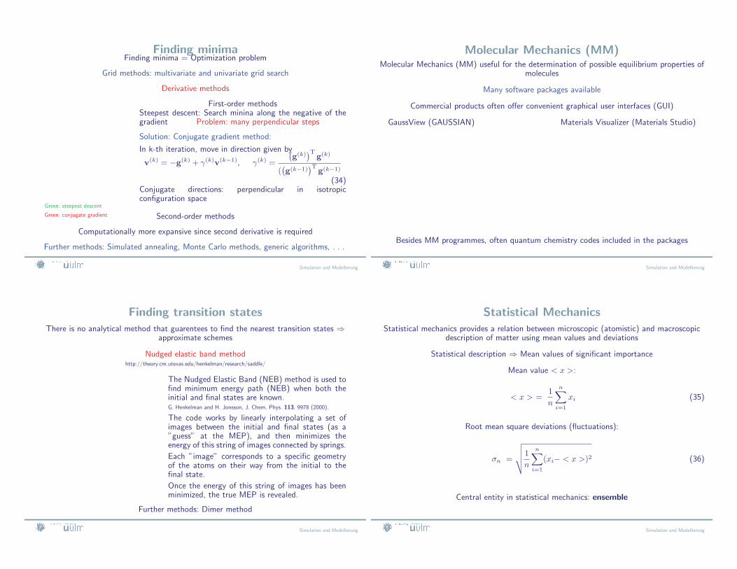
Finding minimaFinding minima = Optimization problem

Grid methods: multivariate and univariate grid search

Derivative methods

Green: steepest descent

Green: conjugate gradient

First-order methodsSteepest descent: Search minina along the negative of thegradient Problem: many perpendicular steps

Solution: Conjugate gradient method:

In k-th iteration, move in direction given by

v(k) = −g(k) + γ(k)v(k−1), γ(k) =

(

g(k))T

g(k)

((

g(k−1))T

g(k−1)

(34)Conjugate directions: perpendicular in isotropicconfiguration space

Second-order methods

Computationally more expansive since second derivative is required

Further methods: Simulated annealing, Monte Carlo methods, generic algorithms, . . .


Finding transition states

There is no analytical method that guarentees to find the nearest transition states ⇒

approximate schemes

Nudged elastic band methodhttp://theory.cm.utexas.edu/henkelman/research/saddle/

The Nudged Elastic Band (NEB) method is used tofind minimum energy path (NEB) when both theinitial and final states are known.G. Henkelman and H. Jonsson, J. Chem. Phys. 113, 9978 (2000).

The code works by linearly interpolating a set ofimages between the initial and final states (as a”guess” at the MEP), and then minimizes theenergy of this string of images connected by springs.

Each ”image” corresponds to a specific geometryof the atoms on their way from the initial to thefinal state.

Once the energy of this string of images has beenminimized, the true MEP is revealed.

Further methods: Dimer method


Molecular Mechanics (MM)Molecular Mechanics (MM) useful for the determination of possible equilibrium properties of

molecules

Many software packages available

Commercial products often offer convenient graphical user interfaces (GUI)

GaussView (GAUSSIAN) Materials Visualizer (Materials Studio)

Besides MM programmes, often quantum chemistry codes included in the packages


Statistical Mechanics

Statistical mechanics provides a relation between microscopic (atomistic) and macroscopicdescription of matter using mean values and deviations

Statistical description ⇒ Mean values of significant importance

Mean value < x >:

< x > =1

n

n∑

i=1

xi (35)

Root mean square deviations (fluctuations):

σn =

√

√

√

√

1

n

n∑

i=1

(xi− < x >)2 (36)

Central entity in statistical mechanics: ensemble


Self-consistent field (SCF) solutionEffective one-particle Hartree-Fock Hamiltonians contain solution: ⇒ SCF iteration scheme

Initial guess:

n0(~r) −→ v

0eff(~r)

?

Solve Schrodinger equations:(

−~2

2m∇

2+ v

jeff

(~r)

)

ψ(j+1)i

(~r) = εiψ(j+1)i

(~r)

?

Determine new density:

n(j+1)

(~r) =

NX

i=1

|ψ(j+1)i

(~r)|2,

and new effective potential vneweff (~r)

?

Do vneweff (~r) and v

jeff

(~r) differ by more than ε ≪ 1?

?

��No

?

Ready

-��Yes

6

Mixing scheme:

v(j+1)eff

(~r) = αvjeff

(~r)

+ (1 − α)vneweff (~r)

with α > 0.9

�


theoretische modellierung und simulation … · theoretische modellierung und simulation ... energy...

Documents