theory and algorithms for reliable multimodal data
TRANSCRIPT
Rochester Institute of Technology Rochester Institute of Technology
RIT Scholar Works RIT Scholar Works
Theses
4-2021
Theory and Algorithms for Reliable Multimodal Data Analysis, Theory and Algorithms for Reliable Multimodal Data Analysis,
Machine Learning, and Signal Processing Machine Learning, and Signal Processing
Dimitris G. Chachlakis [email protected]
Follow this and additional works at: https://scholarworks.rit.edu/theses
Recommended Citation Recommended Citation Chachlakis, Dimitris G., "Theory and Algorithms for Reliable Multimodal Data Analysis, Machine Learning, and Signal Processing" (2021). Thesis. Rochester Institute of Technology. Accessed from
This Dissertation is brought to you for free and open access by RIT Scholar Works. It has been accepted for inclusion in Theses by an authorized administrator of RIT Scholar Works. For more information, please contact [email protected].

Theory and Algorithms for Reliable Multimodal Data Analysis, Machine
Learning, and Signal Processing
by
Dimitris G. Chachlakis
A dissertation submitted in partial fulfillment of the
requirements for the degree of
Doctor of Philosophy in Electrical and Computer Engineering
Kate Gleason College of Engineering
Rochester Institute of Technology
Rochester, New York
April, 2021

Theory and Algorithms for Reliable Multimodal Data Analysis, Machine
Learning, and Signal Processing
by
Dimitris G. Chachlakis
Committee Approval:
We, the undersigned committee members, certify that we have advised and/or supervised the candidate on the work
described in this dissertation. We further certify that we have reviewed the dissertation manuscript and approve it in
partial fulfillment of the requirements of the degree of Doctor of Philosophy in Electrical and Computer Engineering.
Dr. Panos P. Markopoulos Date
Dissertation Advisor
Dr. Sohail Dianat Date
Dissertation Committee Member
Dr. Andreas Savakis Date
Dissertation Committee Member
Dr. Majid Rabbani Date
Dissertation Committee Member
Dr. Nathan Cahill Date
Dissertation Defense Chairperson
Certified by:
Dr. Andres Kwasinski Date
Ph.D. Program Director, Electrical and Computer Engineering
ii

iii
©2021 Dimitris G. Chachlakis
All rights reserved.
Theory and Algorithms for Reliable Multimodal Data Analysis, Machine
Learning, and Signal Processing
by
Dimitris G. Chachlakis
Submitted to theKate Gleason College of Engineering
Ph.D. Program in Electrical and Computer Engineeringin partial fulfillment of the requirements for the degree of
Doctor of Philosophy in Electrical and Computer Engineeringat the Rochester Institute of Technology
Abstract
Modern engineering systems collect large volumes of data measurements across diverse sensing
modalities. These measurements can naturally be arranged in higher-order arrays of scalars which
are commonly referred to as tensors. Tucker decomposition (TD) is a standard method for tensor
analysis with applications in diverse fields of science and engineering. Despite its success, TD
exhibits severe sensitivity against outliers –i.e., heavily corrupted entries that appear sporadically in
modern datasets. We study L1-norm TD (L1-TD), a reformulation of TD that promotes robustness.
For 3-way tensors, we show, for the first time, that L1-TD admits an exact solution via combinatorial
optimization and present algorithms for its solution. We propose two novel algorithmic frameworks
for approximating the exact solution to L1-TD, for general N-way tensors. We propose a novel
algorithm for dynamic L1-TD –i.e., efficient and joint analysis of streaming tensors. Principal-
Component Analysis (PCA) (a special case of TD) is also outlier responsive. We consider Lp-
quasinorm PCA (Lp-PCA) for p < 1, which promotes robustness. Before this dissertation, to the
best of our knowledge, the exact solution to Lp-PCA (p < 1) was unknown. We show, for the first
time, that the problem of one principal component can be solved exactly through a combination of
convex problems and we provide corresponding optimal algorithms. We propose a novel near-exact
algorithm for jointly extracting multiple components. In a different, but related, research direction,
we propose new theory and algorithms for robust Coprime Array (CA) processing. In Direction-
of-Arrival estimation, CAs enable the identification of more sources than sensors by forming the
autocorrelation matrix of a larger virtual uniform linear array which is known as coarray. We
derive closed-form Mean Squared Error (MSE) expressions for the Coarray Autocorrelation Matrix
(CAM) estimation error. We develop a novel approach for estimating the CAM that is designed
under the Minimum-MSE optimality criterion. Finally, we propose a novel CAM estimate which,
in contrast to existing estimates, satisfies the structure-properties of the nominal (true) CAM.
iv

Acknowledgments
This doctorate dissertation would not have been possible without the guidance, support, and as-
sistance that I have received during both my undergraduate and graduate studies.
First, I would like to express my sincerest gratitude to my doctorate dissertation advisor, Dr. Panos
P. Markopoulos, whose invaluable expertise contributed significantly towards the realization of this
dissertation. Thank you for your patience, unconditional support, and opportunities that you have
kindly offered me. Not only have you been a fantastic advisor, but also a mentor who has always
inspired me and endowed me with a remarkable work ethic.
I would also like to thank the members of my dissertation committee, Dr. Sohail Dianat, Dr.
Andreas Savakis, Dr. Majid Rabbani, and Dr. Nathan Cahill, for their invaluable feedback that
helped improve this dissertation, and for the time invested in meetings and reviewing my research.
Further, I want to thank my colleagues at the MILOS Lab for our collaboration and the great
discussions we had throughout the years. I would like to thank my colleague, Mayur Dhanaraj,
with whom I collaborated the most and developed a great friendship.
Moreover, I would like to thank Ms. Rebecca Ziebarth and Dr. Edward Hensel for the tremendous
support and invaluable advise they have offered me whenever it was needed.
I would like to thank the Rochester Institute of Technology, U.S. National Science Foundation,
and U.S. Air Force Research Lab, for funding my research. Also, I would like to thank the U.S.
National Geospatial-Intelligence Agency for co-funding research projects I have worked on.
Notably, I would like to thank my collaborators, Dr. Ashley Prater-Bennette, Dr. Fauzia Ahmad,
and Dr. Evangelos Papalexakis, for the continuous and fruitful collaboration.
I want to thank my undergraduate thesis advisor, Dr. George N. Karystinos, for introducing me to
the world of research and for encouraging me to pursue a Ph.D. degree. Likewise, I would like to
thank Dr. Aggelos Bletsas and Dr. Athanasios Liavas for the excellent work they have been doing
at the Technical University of Crete and for being a great source of inspiration.
At last, I would like to thank my family. I want to thank my father, George and my sister, Maria-
Ioanna for the unconditional support they have selflessly offered me. I also want to thank my
uncle, Charalambos, my aunt, Chrysoula, and my cousins, Konstantinos and Christos, for their
unrelenting support. I also want to thank my loving girlfriend, Rebecca who has been supporting
me in both the good and the bad times. Thank you for the untiring support you have offered me.
v

In memory of my loving mother, Eleni.
vi

Contents
1 Introduction 1
2 L1-norm Tensor Analysis 4
2.1 Introduction . . . . . . . . . . . . . . . . . . . . . . . . . . . . . . . . . . . . . . . . . 4
2.2 Technical Background . . . . . . . . . . . . . . . . . . . . . . . . . . . . . . . . . . . 7
2.3 Problem Statement . . . . . . . . . . . . . . . . . . . . . . . . . . . . . . . . . . . . . 12
2.4 Contribution 1: Exact Solution to Rank-1 L1-norm Tucker2 . . . . . . . . . . . . . . 13
2.4.1 Numerical Studies . . . . . . . . . . . . . . . . . . . . . . . . . . . . . . . . . 21
2.5 Contribution 2: L1-norm HOVSD and L1-norm HOOI for L1-Tucker . . . . . . . . . 22
2.5.1 L1-norm HOSVD Algorithm . . . . . . . . . . . . . . . . . . . . . . . . . . . 22
2.5.2 L1-norm HOOI Algorithm . . . . . . . . . . . . . . . . . . . . . . . . . . . . . 24
2.5.3 Numerical Studies . . . . . . . . . . . . . . . . . . . . . . . . . . . . . . . . . 27
2.6 Contribution 3: Dynamic L1-norm Tucker . . . . . . . . . . . . . . . . . . . . . . . . 38
2.6.1 Dynamic L1-Tucker Algorithm . . . . . . . . . . . . . . . . . . . . . . . . . . 39
2.6.2 Experimental Studies . . . . . . . . . . . . . . . . . . . . . . . . . . . . . . . 44
2.7 Conclusions . . . . . . . . . . . . . . . . . . . . . . . . . . . . . . . . . . . . . . . . . 61
vii

CONTENTS viii
3 Lp-quasinorm Principal-Component Analysis 63
3.1 Introduction . . . . . . . . . . . . . . . . . . . . . . . . . . . . . . . . . . . . . . . . . 63
3.2 Problem Statement . . . . . . . . . . . . . . . . . . . . . . . . . . . . . . . . . . . . . 65
3.3 Contribution 1: The Lp-quasinorm Principal-Component . . . . . . . . . . . . . . . 67
3.3.1 Exact Algorithm 1: Exhaustive Search . . . . . . . . . . . . . . . . . . . . . . 69
3.3.2 Exact Algorithm 2: Search Over Set With Size Polynomial in N . . . . . . . 70
3.4 Contribution 2: The Dominant Lp-PC of a Non-Negative Matrix . . . . . . . . . . . 74
3.5 Contribution 3: Joint Extraction of Multiple Lp-quasinorm Principal-Components . 74
3.6 Contribution 4: Stiefel Manifold Solution Refinement . . . . . . . . . . . . . . . . . . 77
3.7 Numerical Experiments . . . . . . . . . . . . . . . . . . . . . . . . . . . . . . . . . . 81
3.7.1 Subspace Recovery . . . . . . . . . . . . . . . . . . . . . . . . . . . . . . . . . 82
3.7.2 Classification of Biomedical Data . . . . . . . . . . . . . . . . . . . . . . . . . 84
3.8 Conclusions . . . . . . . . . . . . . . . . . . . . . . . . . . . . . . . . . . . . . . . . . 86
4 Coprime Array Processing 87
4.1 Introduction . . . . . . . . . . . . . . . . . . . . . . . . . . . . . . . . . . . . . . . . . 87
4.2 Signal Model and Problem Statement . . . . . . . . . . . . . . . . . . . . . . . . . . 89
4.3 Technical Background . . . . . . . . . . . . . . . . . . . . . . . . . . . . . . . . . . . 92
4.3.1 Selection Combining . . . . . . . . . . . . . . . . . . . . . . . . . . . . . . . . 92
4.3.2 Averaging Combining . . . . . . . . . . . . . . . . . . . . . . . . . . . . . . . 93
4.3.3 Remarks on Existing Coarray Autocorrelation Matrix Estimates . . . . . . . 94
4.4 Contribution 1: Closed-form MSE Expressions for Selection and Averaging Combining 94

CONTENTS ix
4.4.1 Numerical Studies . . . . . . . . . . . . . . . . . . . . . . . . . . . . . . . . . 96
4.5 Contribution 2: Minimum-MSE Autocorrelation Combining . . . . . . . . . . . . . . 99
4.5.1 Numerical Studies . . . . . . . . . . . . . . . . . . . . . . . . . . . . . . . . . 105
4.6 Contribution 3: Structured Coarray Autocorrelation Matrix Estimation . . . . . . . 111
4.6.1 Numerical Studies . . . . . . . . . . . . . . . . . . . . . . . . . . . . . . . . . 115
4.7 Conclusions . . . . . . . . . . . . . . . . . . . . . . . . . . . . . . . . . . . . . . . . . 118
Appendices 138
A Chapter 2 139
A.1 Proof of Convergence for (2.34) . . . . . . . . . . . . . . . . . . . . . . . . . . . . . . 139
A.2 Proof of Lemma 2.4 . . . . . . . . . . . . . . . . . . . . . . . . . . . . . . . . . . . . 140
A.3 Proof of Proposition 2.2 . . . . . . . . . . . . . . . . . . . . . . . . . . . . . . . . . . 141
A.4 Proof of Lemma 2.5 . . . . . . . . . . . . . . . . . . . . . . . . . . . . . . . . . . . . 141
B Chapter 3 142
B.1 Proof of Lemma 3.1 . . . . . . . . . . . . . . . . . . . . . . . . . . . . . . . . . . . . 142
B.2 Proof of Lemma 3.2 . . . . . . . . . . . . . . . . . . . . . . . . . . . . . . . . . . . . 143
B.3 Proof of Lemma 3.3 . . . . . . . . . . . . . . . . . . . . . . . . . . . . . . . . . . . . 143
B.4 Proof of Lemma 3.5 . . . . . . . . . . . . . . . . . . . . . . . . . . . . . . . . . . . . 143
B.5 Proof of Lemma 3.7 . . . . . . . . . . . . . . . . . . . . . . . . . . . . . . . . . . . . 145
B.6 Proof of Proposition 3.2 . . . . . . . . . . . . . . . . . . . . . . . . . . . . . . . . . . 145
B.7 Proof of Lemma 3.9 . . . . . . . . . . . . . . . . . . . . . . . . . . . . . . . . . . . . 146
B.8 Proof of Lemma 3.10 . . . . . . . . . . . . . . . . . . . . . . . . . . . . . . . . . . . . 146

CONTENTS x
B.9 Proof of Proposition 3.4 . . . . . . . . . . . . . . . . . . . . . . . . . . . . . . . . . . 147
C Chapter 4 148
C.1 Proof of Lemma 4.1 . . . . . . . . . . . . . . . . . . . . . . . . . . . . . . . . . . . . 148
C.2 Proof of Lemma 4.2 . . . . . . . . . . . . . . . . . . . . . . . . . . . . . . . . . . . . 149
C.3 Proof of Proposition 4.1 . . . . . . . . . . . . . . . . . . . . . . . . . . . . . . . . . . 149
C.4 Proof of Lemma 4.3 . . . . . . . . . . . . . . . . . . . . . . . . . . . . . . . . . . . . 150
C.5 Proof of Lemma 4.4 . . . . . . . . . . . . . . . . . . . . . . . . . . . . . . . . . . . . 151
C.6 Proof of Proposition 4.2 . . . . . . . . . . . . . . . . . . . . . . . . . . . . . . . . . . 151
C.7 Proof of Lemma 4.5 . . . . . . . . . . . . . . . . . . . . . . . . . . . . . . . . . . . . 151
C.8 Proof of Lemma 4.6. . . . . . . . . . . . . . . . . . . . . . . . . . . . . . . . . . . . . 152
C.9 Proof of Lemma 4.7. . . . . . . . . . . . . . . . . . . . . . . . . . . . . . . . . . . . . 153
C.10 Proof of Remark 4.3 . . . . . . . . . . . . . . . . . . . . . . . . . . . . . . . . . . . . 153
C.11 Proof of Remark 4.5 . . . . . . . . . . . . . . . . . . . . . . . . . . . . . . . . . . . . 154
C.12 Proof of Remark 4.7 . . . . . . . . . . . . . . . . . . . . . . . . . . . . . . . . . . . . 154

List of Figures
2.1 Fitting of HOSVD-derived bases to corrupted fibers, versus corruption variance µ2. . 9
2.2 Schematic illustration of L1-Tucker decomposition for N = 3. . . . . . . . . . . . . 12
2.3 For ρ = 3 and Ns = 4, we draw W ∈ Rρ×N , such that WW> = I3 and Assumption 1
holds true. Then, we plot the nullspaces of all 4 columns of W (colored planes). We
observe that the planes partition R3 into K = 2((
30
)+(
31
)+(
32
)) = 2(1 + 3 + 3) = 14
coherent cells (i.e., 7 visible cells above the cyan hyperplane and 7 cells below.) . . . 18
2.4 Algorithm 2.1 Polynomial in Ns algorithm for the exact solution of rank-1 L1-
Tucker2 in (2.9), with cost O(Nρ+1s ). . . . . . . . . . . . . . . . . . . . . . . . . . . 20
2.5 Reconstruction MSE versus corruption variance σ2c (dB). . . . . . . . . . . . . . . . 21
2.6 Algorithm 2.2 L1-HOSVD algorithm for L1-Tucker (L1HOSVD(X , dnn∈[N ])). . . . 23
2.7 Algorithm 2.3 L1-HOOI algorithm for L1-Tucker (L1HOOI(X , dnn∈[N ])) . . . . . 24
2.8 L1-Tucker metric across L1-HOOI iterations. . . . . . . . . . . . . . . . . . . . . . . 26
2.9 (a) MNSE versus standard deviation σo for No = 300. (b) MNSE versus number of
outliers No for σo = 26. (c) MNSE versus dnn∈[N=5] for No = 150 and σo = 28; for
every m, dm is set to its nominal value and dn variance, n ∈ [5] \m. . . . . . . . . . 29
2.10 MNSE versus λ for varying µ. . . . . . . . . . . . . . . . . . . . . . . . . . . . . . . . 30
2.11 Classification accuracy versus d, for α = 0.2 and β = 0.5. . . . . . . . . . . . . . . . 32
2.12 Classification accuracy versus α, for d = 5 and β = 0.8. . . . . . . . . . . . . . . . . 33
xi

LIST OF FIGURES xii
2.13 Classification accuracy versus β, for α = 0.2 and d = 5. . . . . . . . . . . . . . . . . 33
2.14 Visual illustration (in logarithmic scale) of the 1-st, 7-th, 13-th, and 20-th horizontal
slabs of Xuber. . . . . . . . . . . . . . . . . . . . . . . . . . . . . . . . . . . . . . . . . 35
2.15 Compression error versus compression ratio on the nominal tensor Xuber. . . . . . . 35
2.16 Normalized reconstruction error versus compression ratio in the presence of No = 12
outliers. . . . . . . . . . . . . . . . . . . . . . . . . . . . . . . . . . . . . . . . . . . . 36
2.17 Normalized reconstruction error versus number of outliers. Compression ratio is set
to 182.40 (d = 3). . . . . . . . . . . . . . . . . . . . . . . . . . . . . . . . . . . . . . . 37
2.18 Algorithm 2.4 L1-norm Tucker Decomposition algorithm for batch-processing. . . 39
2.19 A schematic illustration of the proposed algorithm for streaming L1-norm Tucker
decomposition. . . . . . . . . . . . . . . . . . . . . . . . . . . . . . . . . . . . . . . . 40
2.20 Algorithm 2.5 Proposed Dynamic L1-Tucker Decomposition algorithm. . . . . . . 43
2.21 MANSSE vs memory size. N = 3, D = 10, d = 5, B = 5, T = 30, SNR = 0dB,
ONR = 14dB, 3000 realizations. . . . . . . . . . . . . . . . . . . . . . . . . . . . . . 45
2.22 MANSSE vs reliability threshold. N = 3, D = 10, d = 5, B = 5, M = 10, T = 30,
SNR = 0dB, ONR = 14dB, 3000 realizations. . . . . . . . . . . . . . . . . . . . . . . 45
2.23 Frequency of rejection vs reliability threshold. N = 3, D = 10, d = 5, B = 5,
M = 10, T = 30, SNR = 0dB, ONR = 14dB, 3000 realizations. . . . . . . . . . . . . 46
2.24 Frequency of rejection vs outlier probability. N = 3, D = 10, d = 5, B = 5, M = 10,
T = 30, SNR = 0dB, ONR = 14dB, 3000 realizations. . . . . . . . . . . . . . . . . . 46
2.25 Empirical convergence. N = 3, D = 10, d = 3, T = 100, B = 2, M = 12, W = 0,
SNR = −6dB, data-driven τ , 20000 realizations. . . . . . . . . . . . . . . . . . . . . 47
2.26 MANSSE vs update index. N = 3, D = 10, d = 3, T1 = 70, T2 = 30, B = 2,
M = 12, W = 4, SNR = −6dB, ONR = 18dB, data-driven τ , 20000 realizations. . . 48

LIST OF FIGURES xiii
2.27 Reliability and rejection frequency vs update index. N = 3, D = 10, d = 3, T1 = 70,
T2 = 30, B = 2, M = 12, W = 4, SNR = −6dB, ONR = 18dB, data-driven τ , 20000
realizations. . . . . . . . . . . . . . . . . . . . . . . . . . . . . . . . . . . . . . . . . . 49
2.28 Time (sec.) vs update index. N = 3, D = 10, d = 3, T1 = 70, T2 = 30, B = 2,
M = 12, W = 4, SNR = −6dB, ONR = 18dB, data-driven τ , 20000 realizations. . . 50
2.29 MANSSE vs update index. N = 3, D = 10, d = 3, T1 = 75, T2 = 85, B = 2,
M = 12, W = 4, SNR = −6dB, ONR = 18dB, data-driven τ , 20000 realizations. . . 50
2.30 Reliability and rejection frequency vs update index. N = 3, D = 10, d = 3, T1 = 75,
T2 = 85, B = 2, M = 12, W = 4, SNR = −6dB, ONR = 18dB, data-driven τ , 20000
realizations. . . . . . . . . . . . . . . . . . . . . . . . . . . . . . . . . . . . . . . . . . 51
2.31 Dynamic video foreground/background separation experiment. (a) Original 75-th
frame (scene 1). Background extracted by (b) Adaptive Mean (λ = 0.95), (c) DTA
(λ = 0.95), (d) DTA (λ = 0.7), (e) LRUT, (f) OSTD, (g) HOOI (increasing memory),
(h) L1-HOOI (increasing memory), and (i) D-L1-TUCKER (proposed). Foreground
extracted by (j) Adaptive Mean (λ = 0.95), (k) DTA (λ = 0.95), (l) DTA (λ = 0.7),
(m) LRUT, (n) OSTD, (o) HOOI (increasing memory), (p) L1-HOOI (increasing
memory), and (q) D-L1-TUCKER (proposed). . . . . . . . . . . . . . . . . . . . . . 52
2.32 Dynamic video foreground/background separation experiment. (a) Original 150-th
frame (scene 2). Background extracted by (b) Adaptive Mean (λ = 0.95), (c) DTA
(λ = 0.95), (d) DTA (λ = 0.7), (e) LRUT, (f) OSTD, (g) HOOI (increasing memory),
(h) L1-HOOI (increasing memory), and (i) D-L1-TUCKER (proposed). Foreground
extracted by (j) Adaptive Mean (λ = 0.95), (k) DTA (λ = 0.95), (l) DTA (λ = 0.7),
(m) LRUT, (n) OSTD, (o) HOOI (increasing memory), (p) L1-HOOI (increasing
memory), and (q) D-L1-TUCKER (proposed). . . . . . . . . . . . . . . . . . . . . . 53
2.33 Dynamic video foreground/background separation experiment. PSNR (dB) versus
frame index. . . . . . . . . . . . . . . . . . . . . . . . . . . . . . . . . . . . . . . . . . 56
2.34 Online tensor compression and classification experiment. Average classification ac-
curacy versus update index. . . . . . . . . . . . . . . . . . . . . . . . . . . . . . . . . 56

LIST OF FIGURES xiv
2.35 Frame instances per scene for the three videos. Video 1: (a) scene 1, (b) scene 2,
and (c) noisy frame. Video 2: (d) scene 1, (e) scene 2, and (f) noisy frame. Video
3: (g) scene 1, (h) scene 2, and (i) noisy frame. Probability of noise corruption per
pixel is 10% for all noisy frames. . . . . . . . . . . . . . . . . . . . . . . . . . . . . . 58
2.36 Average online video scene change detection accuracy versus probability of noise
corruption per pixel. For videos 1 and 3, the probability of frame corruption pf is
set to 0.1 while for video 2 it is set to 0.25. Video 1 (left), video 2 (middle), and
video 3 (right). . . . . . . . . . . . . . . . . . . . . . . . . . . . . . . . . . . . . . . . 59
2.37 Online anomaly detection. B = 5, M = 5, d = 10, 300 realizations, data-driven τ . . . 62
3.1 Metric surface of ‖X>q‖pp for arbitrary X ∈ R2×5 and p ∈ 2, 1, 0.5. . . . . . . . . . 67
3.2 Metric surface of ‖X>q‖pp for p = 0.5 and arbitrary X ∈ R2×5 when q scans C(b)
for fixed b. . . . . . . . . . . . . . . . . . . . . . . . . . . . . . . . . . . . . . . . . . 68
3.3 CVX code (Matlab) for the solution to (3.4). . . . . . . . . . . . . . . . . . . . . . . 68
3.4 Algorithm 3.1 Exhaustive search for the exact solution to Lp-PCA. . . . . . . . . . 69
3.5 Partition of the hypersphere/hyperball to a set of halfspaces-intersection “cells” for
an arbitrary X ∈ R(D=3)×(N=4). . . . . . . . . . . . . . . . . . . . . . . . . . . . . . . 70
3.6 Algorithm 3.2 Exact Lp-PCA via search over polynomial (in N) size set. . . . . . 71
3.7 CVX code (Matlab) for the solution to (3.24). . . . . . . . . . . . . . . . . . . . . . . 75
3.8 Algorithm 3.3 Multiple Lp-PCs (convex relaxation) via search over polynomial (in
N) size set. . . . . . . . . . . . . . . . . . . . . . . . . . . . . . . . . . . . . . . . . . 77
3.9 Evaluation of the proposed iteration in (3.29) for p = 1, D = 3, N = 5, and K = 2.
Reported curve-values are averages over 30 realizations of data. . . . . . . . . . . . . 79
3.10 Evaluation of the proposed iteration in (3.29) for p = 0.90, D = 3, N = 5, and
K = 2. Reported curve-values are averages over 30 realizations of data. . . . . . . . 79
3.11 Evaluation of the proposed iteration in (3.29) for p = 0.75, D = 3, N = 5, and
K = 2. Reported curve-values are averages over 30 realizations of data. . . . . . . . 80

LIST OF FIGURES xv
3.12 Evaluation of the proposed iteration in (3.29) for p = 1, D = 4, N = 5, and K = 3.
Reported curve-values are averages over 30 realizations of data. . . . . . . . . . . . . 80
3.13 Evaluation of the proposed iteration in (3.29) for p = 0.90, D = 4, N = 5, and
K = 3. Reported curve-values are averages over 30 realizations of data. . . . . . . . 81
3.14 Evaluation of the proposed iteration in (3.29) for p = 0.75, D = 4, N = 5, and
K = 3. Reported curve-values are averages over 30 realizations of data. . . . . . . . 81
3.15 Subspace recovery: NSSE vs number of outliers No. D = 7, N = 7, K = 1, p = 0.5,
SNR = 8dB, ONR = 18dB. . . . . . . . . . . . . . . . . . . . . . . . . . . . . . . . . 82
3.16 Subspace recovery: NSSE vs ONR (dB). D = 7, N = 7, K = 1, p = 0.25, SNR
= 8dB, No = 2. . . . . . . . . . . . . . . . . . . . . . . . . . . . . . . . . . . . . . . . 83
3.17 Subspace recovery: NSSE vs p. D = 7, N = 7, K = 1, ONR = 18dB , SNR = 8dB,
No = 2. . . . . . . . . . . . . . . . . . . . . . . . . . . . . . . . . . . . . . . . . . . . 83
3.18 Breast Cancer Wisconsin (Diagnostic) Dataset: Classification accuracy vs p. Ntrain =
20, Ntest = 100, m = 0. . . . . . . . . . . . . . . . . . . . . . . . . . . . . . . . . . . . 85
3.19 Breast Cancer Wisconsin (Diagnostic) Dataset: Classification accuracy vs p. Ntrain =
20, Ntest = 100, m = 3. . . . . . . . . . . . . . . . . . . . . . . . . . . . . . . . . . . . 85
3.20 Breast Cancer Wisconsin (Diagnostic) Dataset: Classification accuracy vs number
of mislabelings. Ntrain = 20, Ntest = 100, p = 0.1. . . . . . . . . . . . . . . . . . . . . 86
4.1 Coprime processing steps: from a collection of samples yqQq=1 to the estimated
coarray signal-subspace basis U. . . . . . . . . . . . . . . . . . . . . . . . . . . . . . 92
4.2 Theoretically and numerically calculated MSEs errZ(Zsel) and errZ(Zavg), versus
sample-support Q. . . . . . . . . . . . . . . . . . . . . . . . . . . . . . . . . . . . . . 97
4.3 Theoretically and numerically calculated MSEs errZ(Zsel) and errZ(Zavg), versus the
number of transmitting sources K. . . . . . . . . . . . . . . . . . . . . . . . . . . . . 97
4.4 Average squared subspace error attained by selection and averaging sampling, versus
sample-support Q. . . . . . . . . . . . . . . . . . . . . . . . . . . . . . . . . . . . . . 98
LIST OF FIGURES xvi
4.5 RMSE of coprime MUSIC DoA estimation attained by selection and averaging sam-
pling, versus sample-support Q. . . . . . . . . . . . . . . . . . . . . . . . . . . . . . . 98
4.6 Probability density function f(θ) for different distributions and support sets. . . . . 101
4.7 Empirical CDF of the MSE in estimating Z for (M,N) = (2, 3), SNR= 10dB,Q = 10,
K = 5 (top), and K = 7 (bottom). ∀k, θk ∼ U(−π2 ,
π2 ) (left), U(−π
4 ,π6 ) (center),
T N (−π8 ,
π8 , 0, 1) (right). . . . . . . . . . . . . . . . . . . . . . . . . . . . . . . . . . . 106
4.8 Empirical CDF of the NMSE in estimating Z for (M,N) = (2, 5), SNR= 10dB,
Q = 10, K = 7 (top), and K = 9 (bottom). ∀k, θk ∼ U(−π2 ,
π2 ) (left), U(−π
4 ,π6 )
(center), and T N (−π8 ,
π8 , 0, 1) (right). . . . . . . . . . . . . . . . . . . . . . . . . . . 107
4.9 NMSE in estimating Z, versus sample support, Q. (M,N) = (2, 5), SNR= 10dB,
and K = 7. ∀k, θk ∼ U(−π2 ,
π2 ) (left), U(−π
4 ,π6 ) (center), T N (−π
8 ,π8 , 0, 1) (right). . . 108
4.10 RMSE (degrees) in estimating the DoA set Θ, versus sample support, Q. (M,N) =
(2, 5), SNR= 10dB, and K = 7. ∀k, θk ∼ U(−π2 ,
π2 ) (left), U(−π
4 ,π6 ) (center),
T N (−π8 ,
π8 , 0, 1) (right). . . . . . . . . . . . . . . . . . . . . . . . . . . . . . . . . . . 108
4.11 RMSE (degrees) in estimating the DoA set Θ, versus sample support, Q. (M,N) =
(3, 5) andK = 11. (Θ, SNR,D(a, b)) = (Θ1, 0dB,U(−π2 ,
π2 )) –top left, (Θ1, 8dB,U(−π
2 ,π2 ))
–bottom left, (Θ2, 0dB,U(−π4 ,
π4 )) –top center, (Θ2, 8dB,U(−π
4 ,π4 )) –bottom center,
(Θ3, 0dB,U(−π4 ,
π6 )) –top right, (Θ3, 8dB,U(−π
4 ,π6 )) –bottom right. . . . . . . . . . . 109
4.12 Illustration of the ith diagonal of X ∈ C4×4, di(X), i ∈ 0,±2. . . . . . . . . . . . . 112
4.13 Illustration of Proposition 4.3. (M,N) = (2, 3), Θ = −43,−21,−10, 17, 29, 54,dk = 0dB ∀k, σ2 = 1, Q = 50. . . . . . . . . . . . . . . . . . . . . . . . . . . . . . . . 113
4.14 Algorithm 4.1 Structured coarray autocorrelation matrix estimation . . . . . . . . . . . 114
4.15 Root Mean Normalized Squared Error (RMNSE) with respect to (w.r.t.) Rco, Root
Mean Normalized - Subspace Squared Error (RMN-SSE) w.r.t. Qco, and Root Mean
Squared Error (RMSE) w.r.t. Θ vs sample support for varying SNR ∈ −4, 2dB. . . 117
List of Tables
2.1 Computational costs of PCA, L1PCA-FPI, HOSVD, L1-HOSVD (proposed), HOOI,
and L1-HOOI (proposed). PCA/L1PCA-FPI costs are reported for input matrix
X ∈ RD×D and decomposition rank d. Tucker/L1-Tucker costs are reported for N -
way input tensor X ∈ RD×D×...×D and mode-n ranks dn = d ∀n. T is the maximum
number of iterations conducted by HOOI and L1-HOOI. . . . . . . . . . . . . . . . . 28
4.1 Entry-wise closed-form expression for matrix V defined in (4.22). . . . . . . . . . . . 102
4.2 Closed-form expression for γ(i,m)j defined in (4.33) . . . . . . . . . . . . . . . . . . . . 103
4.3 Closed-form expression for EΘγ(i,m)j . . . . . . . . . . . . . . . . . . . . . . . . . . . 103
4.4 Comparison of coarray autocorrelation matrix estimates: autocorrelation sampling
approach and structure properties. . . . . . . . . . . . . . . . . . . . . . . . . . . . . 115
xvii

Chapter 1
Introduction
In this doctorate dissertation, we propose new theory and algorithms for multimodal (tensor) data
analysis, machine learning, and sparse array processing.
Modern engineering systems collect large volumes of data measurements across diverse sensing
modalities. These measurements can naturally be arranged in higher-order arrays of scalars which
are commonly referred to as multiway arrays or tensors. For instance, a 1-way tensor is a standard
vector, a 2-way tensor is a standard matrix, and a 3-way array is a data cube of scalars. For higher-
order tensors, visualization is not a trivial task and is left to the imagination. Storing, processing,
and analyzing tensor data in their natural form enables the discovery of patterns and underlying
data structures that would have otherwise stayed hidden. This is often attributed to the fact that
tensors naturally model higher-order correlations among the data. Tucker Decomposition (TD)
and Canonical Polyadic Decomposition (CPD) are the most popular tensor analysis approaches
in the literature. TD focuses more on compression and multilinear subspace analysis while CPD
aims at extracting sets of non-rotatable features that promote interpretability. Both TD and CPD
find applications in diverse fields of science and engineering. In this dissertation, we focus on TD.
Despite its success, TD exhibits severe sensitivity against outliers –i.e., heavy magnitude peripheral
entries within the processed tensor. Accordingly, applications the performance of which relies on
TD may attain compromised performance. We consider outlier resistant reformulations of TD, set
the theoretical foundations for these formulations, and propose new algorithms.
Principal-Component Analysis (PCA) –a special case of TD– is a standard method for data analysis
with a plethora of applications among fields of science and engineering. Similar to TD, it has been
well documented that PCA is outlier-responsive. Thus, applications that rely on PCA may attain
1
CHAPTER 1. INTRODUCTION 2
compromised performance when outliers are found among the processed data. To remedy the
impact of outliers, researchers have proposed an array or outlier resistant reformulations of PCA.
Arguably, L1-norm PCA (L1-PCA), which derives by simple substitution of the L2-norm in the
PCA formulation by the more robust L1-norm, is the most straightforward one. This change in
norm promotes robustness. L1-PCA is, in fact, a special case of the general Lp-norm PCA (Lp-
PCA) formulation for p = 1. For general values of p ≤ 1, before this dissertation, to the best
of our knowledge, the exact solution to Lp-PCA was unknown. In this dissertation, we focus on
the special case that p ≤ 1 and pursue the exact solution to Lp-quasinorm Principal-Component
Analysis.
In a different, but related, research direction, we propose new theory and estimation algorithms
for robust coprime array processing. Coprime Arrays (CAs) are sparse arrays which offer an
increased number of Degrees-of-Freedom (DoF) when compared to equal-length Uniform Linear
Arrays (ULAs). CAs have attracted significant research interest over the past years and have been
successfully employed in numerous modern applications.
The main contributions of this dissertation are organized in the following Chapters.
In Chapter 2, we develop theory and algorithms for reliable tensor data analysis. Standard tensor
analysis approaches in the literature are formulated based on the L2/Frobenius norm which has
been shown to exhibit severe sensitivity against peripheral heavy-magnitude/tail noise points. We
consider L1-norm tensor analysis formulations and set the theoretical foundations that allow us
to develop, for the first time, exact and approximate algorithms that are accompanied by formal
complexity and convergence analyses. Furthermore, we also consider the problem of streaming
tensor data and develop a new scalable algorithm that remains robust against outliers. The merits
of L1-norm tensor analysis are clearly documented in an extensive array of numerical experiments
with both synthetic and real-world datasets.
Next, in Chapter 3, we study the problem of Lp-quasinorm Principal-Component Analysis (Lp-
PCA) for p ≤ 1. Before this dissertation, to the best of our knowledge, the solution to Lp-PCA
was unknown. We show, for the first time, that the problem of one principal component can be
solved exactly through a combination of convex problems and we provide corresponding optimal
algorithms. Moreover, we propose a novel near-exact algorithm for jointly extracting multiple com-
ponents. Extensive numerical studies on both synthetic and real-world medical datasets corroborate
the merits of Lp-PCA compared to the standard PCA.
Finally, in Chapter 4, we steer our focus on sparse array processing. Briefly, processing at a spare

CHAPTER 1. INTRODUCTION 3
array receiver can be summarized in the following steps: physical-array autocorrelation estima-
tion, autocorrelation combining, and spatial smoothing, after which an autocorrelation matrix that
corresponds to a larger virtual uniform linear array is formed. We specifically focus on the auto-
correlation combining step and develop new theory and a novel autocorrelation combining method
that relies on the Minimum-Mean-Squared-Error optimality criterion. In addition, we propose an
algorithm for computing improved autocorrelation estimates, compared to standard counterparts,
by leveraging known structure properties that derive from the received-signal model. The new
theory is validated by means of numerical simulations. The performances of the new autocorrela-
tion combining approach and the new autocorrelation matrix estimate are evaluated by means of
extensive numerical experiments.

Chapter 2
L1-norm Tensor Analysis
2.1 Introduction
Data collections across diverse sensing modalities are naturally stored and processed in the form
of N -way arrays, also known as tensors. Introduced by L. R. Tucker [1] in the mid-1960s, Tucker
decomposition (TD) is a standard method for the analysis and compression of tensor data. TD finds
a plethora of applications across fields of science and engineering, such as communications [2–6],
data analytics [7, 8], machine learning [9–14], computer vision [15–20], biomedical signal processing
[21], social-network data analysis [22, 23], and pattern recognition [24, 25], among other fields. TD
is typically used for compression, denoising, and model identification, to name a few. Notably,
an alternative paradigm for tensor analysis, particularly popular for data mining, is the Canonical
Polyadic Decomposition (CPD), also referred to as Parallel Factor Analysis (PARAFAC) [8, 26].
In contrast to TD that focuses more on compression and multilinear subspace analysis, CPD aims
at extracting sets of non-rotatable features that promote interpretability.
In many applications of interest, an N -way data tensor is formed by concatenation of (N − 1)-
way coherent (same class, or distribution) tensor samples across its, without loss of generality
(w.l.o.g), N -th mode –i.e., the data tensor comprises (N − 1) feature modes and 1 sample mode.
For such applications, TD is accordingly reformulated to Tucker2 decomposition (T2D) [27], which
can be described as joint TD of the (N − 1)-way tensor samples. That is, T2D strives to jointly
decompose the collected (N − 1)-way tensors and unveil the low-rank multilinear structure of their
class, or distribution. For the special case that N = 3 (collection of matrix or 2-way measurements),
TD/T2D take the familiar form of Principal-Component Analysis (PCA). For the same case, T2D
4

CHAPTER 2. L1-NORM TENSOR ANALYSIS 5
has also been presented as Generalized Low-Rank Approximation of Matrices (GLRAM) [28, 29],
or 2-D Principal Component Analysis (2DPCA) [18, 30]. For N = 2 (collection of vector samples),
both TD and T2D boil down to standard matrix Principal-Component Analysis (PCA), computable
by means of Singular-Value Decomposition (SVD) [31].
In general, conventional TD tries to minimize the L2-norm of the residual-error in the low-rank
approximated tensor that derives by multi-way projection of the original tensor onto the spans of N
sought-after orthonormal bases –or, equivalently, TD tries to maximize the L2-norm of this multi-
way projection. Higher-Order SVD (HOSVD) and Higher-Order Orthogonal Iteration (HOOI)
algorithms [32] are well-known solvers for TD and T2D. Note that both types of solvers can gen-
erally only guarantee a locally optimal solution. Furthermore, a plethora of TD variants have also
been presented in the literature. Truncated HOSVD (T-HOSVD) [33, 34], Sequentially Truncated
HOSVD (ST-HOSVD) [35], Hierarchical HOSVD [36], and Nonnegative Tucker [37, 38], are just a
few.
TD and T2D have also been studied for applications in which the tensor measurements arrive in a
streaming way. In such applications, the sought-after TD bases have to be computed incrementally.
Incremental solvers are also preferred, from a computational standpoint, when there are too many
collected measurements to efficiently process them as a batch. Researchers have proposed an array
of algorithms for incremental TD, including Dynamic Tensor Analysis (DTA), Streaming Tensor
Analysis (STA), Window-based Tensor Analysis (WTA) [39, 40], and Accelerated Online Low-Rank
Tensor Learning (ALTO) [41], to name a few. Scalable, parallelized, streaming, and randomized
algorithms for TD have also been proposed in [42–46].
The merits of TD have been demonstrated in a wide range of applications. However, it is well
documented that TD is very sensitive against faulty measurements (outliers). Outliers appear
often in modern datasets due to sensor malfunctions, errors in data storage/transfer, and even
deliberate dataset contamination in adversarial environments [47–52]. The same sensitivity has
also been amply documented in PCA/SVD, which is a special case of TD for 2-way tensors. For
the case of matrix decomposition, researchers have shown that the impact of faulty entries can be
effectively counteracted by substituting SVD with L1-norm-based PCA (L1-PCA) [53, 54]. L1-
PCA is formulated similar to standard PCA as a projection maximization problem, but replaces
the corruption-responsive L2-norm by the robust L1-norm. L1-PCA has exhibited solid robustness
against heavily corrupted data in an array of applications [55–58]. Extending this formulation to
tensor processing, one can similarly endow robustness to the TD and T2D by substituting the
L2-norm in their formulations by the L1-norm (not to be confused with sparsity-inducing L1-norm

CHAPTER 2. L1-NORM TENSOR ANALYSIS 6
regularization schemes). An approximate algorithm for L1-norm-based Tucker2 (L1-T2D) was
proposed in [52] for the special case that N = 3 and data are processed as a batch. However,
L1-T2D and L1-TD remain to date unsolved and largely unexplored.
In this Chapter, we study the theoretical foundations of L1-norm TD and T2D and develop algo-
rithms for their solutions. Specifically, our contributions are as follows:
Contribution i. We deliver, for the first time, the exact solution to rank-1 L1-T2D decomposition
by means of two novel algorithms.
Contribution ii. We present generalized L1-TD decomposition for N -way tensors and review
its links to PCA, TD/T2D, and L1-PCA. We propose two new algorithmic
frameworks for the solution of L1-TD/L1-T2D, namely L1-norm Higher-Order
SVD (L1-HOSVD) and L1-norm Higher-Order Orthogonal Iterations (L1-HOOI),
which are accompanied by complete convergence and complexity analyses.
Contribution iii. We present Dynamic L1-Tucker: a scalable method for incremental L1-TD anal-
ysis, with the ability to (1) provide quality estimates of the Tucker bases, (2)
detect and reject outliers, and (3) adapt to changes of the nominal subspaces.
Contribution iv. In all the above cases, we offer numerical studies that evaluate the performance of
L1-TD and compare it with state-of-the-art counterparts. Our numerical studies
corroborate that L1-TD performs similar to standard TD when the processed
data are nominal/clean, while it exhibits sturdy resistance against corruptions
among the data.
The rest of this Chapter is organized as follows. In Section 2.2, we introduce notation and review
existing tensor analysis methods. Next, in Section 2.3, we present the general formulation of L1-
norm Tucker (L1-Tucker) analysis. In Section 2.4, we present, for the first time, the exact solution
to rank-1 L1-norm Tucker2 Analysis. Thereafter, in Section 2.5, we offer the proposed L1-HOSVD
and L1-HOOI algorithmic frameworks for the solution to L1-Tucker/L1-Tucker2. In Section 2.6,
we present Dynamic L1-Tucker (D-L1-Tucker) for incremental and dynamic analysis of streaming
tensor measurements.
The contributions presented in this Chapter have also been presented in [59–65].
CHAPTER 2. L1-NORM TENSOR ANALYSIS 7
2.2 Technical Background
Notation and Tensor Preliminaries
In this Chapter, vectors and matrices are denoted by lower- and upper-case bold letters, respectively
–e.g., x ∈ RD1 and X ∈ RD1×D2 . N -way tensors are denoted by upper-case calligraphic bold letters
–e.g., X ∈ RD1×...×DN . An N -way tensor X ∈ RD1×D2×...×DN can also be viewed as an M -way
tensor in RD1×D2×...×DM , for any M > N , with Dm = 1 for m > N . Collections/sets of tensors are
denoted by upper-case calligraphic letters –e.g., X = X ,Y. The squared Frobenius/L2 norm,
‖ · ‖2F , returns the sum of squared entries of its tensor argument while the L1-norm, ‖ · ‖1, returns
the sum of the absolute entries of its tensor argument. SD×d = Q ∈ RD×d : Q>Q = Id is
the Stiefel manifold of rank-d orthonormal matrices in RD. Each entry of X is identified by N
indices inNn=1 such that in ≤ Dn for every n ∈ [N ] = 1, 2, . . . , N. For every n ∈ [N ], X can
be seen as a collection of Pn =∏m∈[N ]\nDm length-Dn vectors known as mode-n fibers of X . For
instance, given a fixed set of indices im∈[N ]\n, X (i1, . . . , in−1, :, in+1, . . . , iN ) is a mode-n fiber of
X . A matrix that has as columns all the mode-n fibers of X is called the mode-n unfolding (or,
flattening) of X and will henceforth be denoted as mat(X , n) ∈ RDn×Pn . The reverse procedure,
known as mode-n “tensorization”, rearranges the entries of matrix X ∈ RDn×Pn to form tensor
ten(X;n; Dii 6=n) ∈ RD1×D2×...×DN , so that mat(ten(X;n; Dii 6=n), n) = X. X ×n A is the
mode-n product of tensor X with matrix A of conformable size and X×n∈[N ]Q>n compactly denotes
the multi-way product X ×1 Q>1 ×2 Q>2 . . .×nQ>N . In accordance with the common convention, the
order in which the mode-n fibers of X appear in mat(X , n) is as specified in [66]. For more details
on tensor preliminaries, we refer the interested reader to [12, 66].
Tucker Decomposition
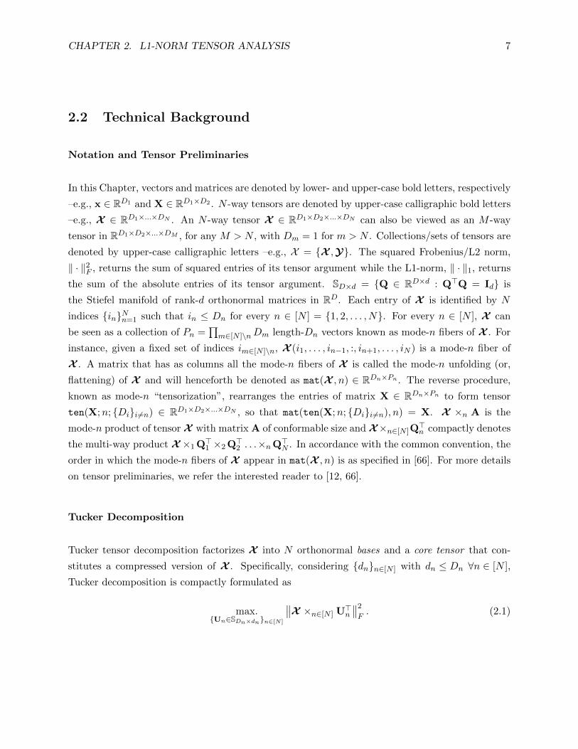
Tucker tensor decomposition factorizes X into N orthonormal bases and a core tensor that con-
stitutes a compressed version of X . Specifically, considering dnn∈[N ] with dn ≤ Dn ∀n ∈ [N ],
Tucker decomposition is compactly formulated as
max.Un∈SDn×dnn∈[N ]
∥∥X ×n∈[N ] U>n∥∥2
F. (2.1)
CHAPTER 2. L1-NORM TENSOR ANALYSIS 8
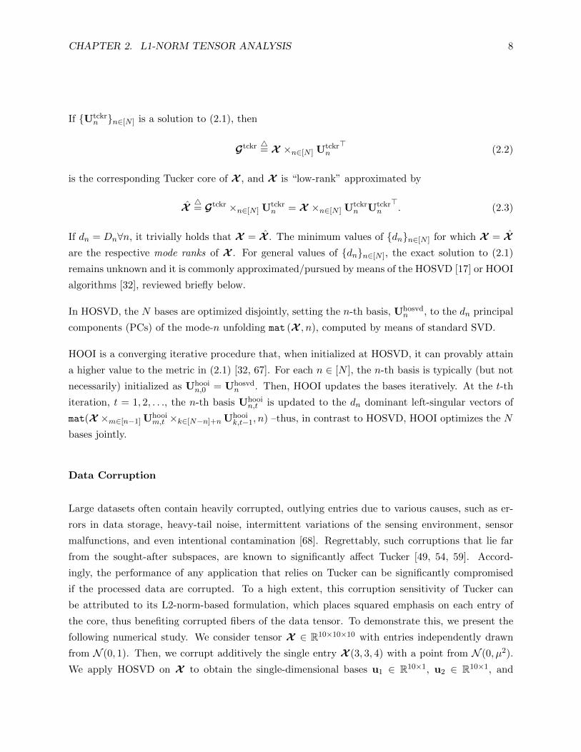
If Utckrn n∈[N ] is a solution to (2.1), then
Gtckr 4= X ×n∈[N ] Utckrn>
(2.2)
is the corresponding Tucker core of X , and X is “low-rank” approximated by
X 4= Gtckr ×n∈[N ] Utckr
n = X ×n∈[N ] Utckrn Utckr
n>. (2.3)
If dn = Dn∀n, it trivially holds that X = X . The minimum values of dnn∈[N ] for which X = Xare the respective mode ranks of X . For general values of dnn∈[N ], the exact solution to (2.1)
remains unknown and it is commonly approximated/pursued by means of the HOSVD [17] or HOOI
algorithms [32], reviewed briefly below.
In HOSVD, the N bases are optimized disjointly, setting the n-th basis, Uhosvdn , to the dn principal
components (PCs) of the mode-n unfolding mat (X , n), computed by means of standard SVD.
HOOI is a converging iterative procedure that, when initialized at HOSVD, it can provably attain
a higher value to the metric in (2.1) [32, 67]. For each n ∈ [N ], the n-th basis is typically (but not
necessarily) initialized as Uhooin,0 = Uhosvd
n . Then, HOOI updates the bases iteratively. At the t-th
iteration, t = 1, 2, . . ., the n-th basis Uhooin,t is updated to the dn dominant left-singular vectors of
mat(X ×m∈[n−1] Uhooim,t ×k∈[N−n]+n Uhooi
k,t−1, n) –thus, in contrast to HOSVD, HOOI optimizes the N
bases jointly.
Data Corruption
Large datasets often contain heavily corrupted, outlying entries due to various causes, such as er-
rors in data storage, heavy-tail noise, intermittent variations of the sensing environment, sensor
malfunctions, and even intentional contamination [68]. Regrettably, such corruptions that lie far
from the sought-after subspaces, are known to significantly affect Tucker [49, 54, 59]. Accord-
ingly, the performance of any application that relies on Tucker can be significantly compromised
if the processed data are corrupted. To a high extent, this corruption sensitivity of Tucker can
be attributed to its L2-norm-based formulation, which places squared emphasis on each entry of
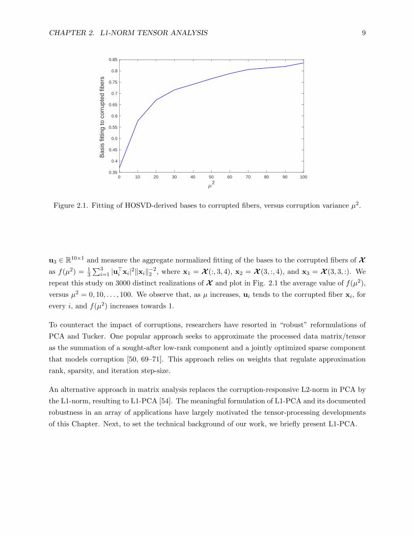
the core, thus benefiting corrupted fibers of the data tensor. To demonstrate this, we present the
following numerical study. We consider tensor X ∈ R10×10×10 with entries independently drawn
from N (0, 1). Then, we corrupt additively the single entry X (3, 3, 4) with a point from N (0, µ2).
We apply HOSVD on X to obtain the single-dimensional bases u1 ∈ R10×1, u2 ∈ R10×1, and
CHAPTER 2. L1-NORM TENSOR ANALYSIS 9
0 10 20 30 40 50 60 70 80 90 1002
0.35
0.4
0.45
0.5
0.55
0.6
0.65
0.7
0.75
0.8
0.85
Bas
is fi
tting
to c
orru
pted
fibe
rs
Figure 2.1. Fitting of HOSVD-derived bases to corrupted fibers, versus corruption variance µ2.
u3 ∈ R10×1 and measure the aggregate normalized fitting of the bases to the corrupted fibers of Xas f(µ2) = 1
3
∑3i=1 |u>i xi|2‖xi‖−2
2 , where x1 = X (:, 3, 4), x2 = X (3, :, 4), and x3 = X (3, 3, :). We
repeat this study on 3000 distinct realizations of X and plot in Fig. 2.1 the average value of f(µ2),
versus µ2 = 0, 10, . . . , 100. We observe that, as µ increases, ui tends to the corrupted fiber xi, for
every i, and f(µ2) increases towards 1.
To counteract the impact of corruptions, researchers have resorted in “robust” reformulations of
PCA and Tucker. One popular approach seeks to approximate the processed data matrix/tensor
as the summation of a sought-after low-rank component and a jointly optimized sparse component
that models corruption [50, 69–71]. This approach relies on weights that regulate approximation
rank, sparsity, and iteration step-size.
An alternative approach in matrix analysis replaces the corruption-responsive L2-norm in PCA by
the L1-norm, resulting to L1-PCA [54]. The meaningful formulation of L1-PCA and its documented
robustness in an array of applications have largely motivated the tensor-processing developments
of this Chapter. Next, to set the technical background of our work, we briefly present L1-PCA.

CHAPTER 2. L1-NORM TENSOR ANALYSIS 10
The L1-PCA Paradigm
Given a data matrix X ∈ RD1×D2 and d1 ≤ rank(X), L1-PCA is defined as [54]
max.U∈SD1×d1
‖U>X‖1, (2.4)
where the L1-norm ‖ · ‖1 returns the summation of the absolute entries of its matrix argument.
L1-PCA in (2.4) was solved exactly in [54], where authors presented the following Theorem 2.1.
Theorem 2.1. Let Bnuc be an optimal solution to
max.B∈±1D2×d1
‖XB‖∗. (2.5)
Then, UL1 = Φ(XBnuc) is an optimal solution to L1-PCA in (2.4). Moreover, ‖X>UL1‖1 =
Tr(U>L1XBnuc
)= ‖XBnuc‖∗.
Nuclear norm ‖·‖∗ in (2.5) returns the sum of the singular values of its matrix argument. For any tall
matrix A ∈ Rm×n that admits SVD WSn×nQ>, Φ(·) in Theorem 2.1 is defined as Φ(A)
4= WQ>.
Moreover, by the Procrustes Theorem [72], it holds that Φ(A) = argmaxU∈Sm×n Tr(U>A) =
argminU∈Sm×n ‖U−A‖F .
By means of Theorem 2.1, the solution to L1-PCA is obtained by solving the Binary Nuclear-norm
Maximization (BNM) in (2.5), with an additional SVD step. BNM can be solved by exhaustive
search in its finite-size feasibility set, or more intelligent algorithms of lower cost, as shown in [54].
Computationally efficient, approximate solvers for (2.5) and (2.4) were presented in [55, 58, 73–76].
Incremental solvers for L1-PCA were presented in [77, 78]. Algorithms for L1-PCA of complex-
valued data were recently presented in [79, 80]. To date, L1-PCA has found many applications in
signal processing and machine learning, such as radar-based motion recognition and foreground-
activity extraction in video sequences [56, 57].
Existing Methods for Incremental and Dynamic Tucker
Streaming and robust matrix PCA has been thoroughly studied over the past decades [77, 81–85].
However, extending matrix PCA (batch or streaming) to tensor analysis is a non-trivial task that
has been attracting increasing research interest. To date, there exist multiple alternative methods
for batch tensor analysis (e.g., HOSVD, HOOI, L1-HOOI) but only few for streaming/dynamic

CHAPTER 2. L1-NORM TENSOR ANALYSIS 11
tensor analysis. For example, DTA [39, 40] efficiently approximates the HOSVD solution by pro-
cessing measurements incrementally, with a fixed computational cost per update. Moreover, DTA
can track multilinear changes of subspaces, weighing past measurements with a forgetting factor.
STA [39, 40] is a fast alternative to DTA, particularly designed for time-critical applications. WTA
is another DTA variant which, in contrast to DTA and STA, adapts to changes by considering only
a sliding window of measurements. The ALTO method was presented in [41]. For each new mea-
surement, ALTO updates the bases through a tensor regression model. In [86], authors presented
another method for Low-Rank Updates to Tucker (LRUT). When a new measurement arrives,
LRUT projects it on the current bases and few more randomly chosen orthogonal directions, form-
ing an augmented core tensor. Then it updates the bases by standard Tucker (e.g., HOSVD) on this
extended core. In [45], authors consider very large tensors and propose randomized algorithms for
Tucker decomposition based on the TENSORSKETCH [87]. It is stated that these algorithms can
also extend for processing streaming data. Randomized methods for Tucker of streaming tensor
data were also proposed in [42]. These methods rely on dimension-reduction maps for sketch-
ing the Tucker decomposition and they are accompanied by probabilistic performance guarantees.
More methods for incremental tensor processing were presented in [88–91], focusing on specific
applications such as foreground segmentation, visual tracking, and video foreground/background
separation.
Methods for incremental CPD/PARAFAC tensor analysis have also been presented. For instance,
authors in [92] consider the CPD/PARAFAC factorization model and assume that N -way mea-
surements are streaming. They propose CP-Stream, an algorithm that efficiently updates the CPD
every time a new measurement arrives. CP-stream can accommodate user-defined constraints in the
factorization such as non-negativity. In addition, authors in [93] consider a Bayesian probabilistic
reformulation of the CPD/PARAFAC factorization, assuming that the entries of the processed ten-
sor are streaming across all modes, and develop a posterior inference algorithm (POST). Further,
the problem of robust and incremental PARAFAC has also been studied and algorithms have been
presented in [94, 95]. Typically, the application spaces of CPD and TD are complementary: CPD
is preferred when uniqueness and interpretability are needed; Tucker allows for the latent compo-
nents to be related (dense core) and it is preferred for low-rank tensor compression and completion,
among other tasks [8, 14].

CHAPTER 2. L1-NORM TENSOR ANALYSIS 12
! "U1
U2 U3
Original tensor datacompressed data
1
2 3
L1-Tuckerbases
L1-Tucker core /
Figure 2.2. Schematic illustration of L1-Tucker decomposition for N = 3.
2.3 Problem Statement
Motivated by the corruption resistance of L1-PCA, we study L1-Tucker decomposition. L1-Tucker
derives by simply replacing the L2-norm in (2.1) by the corruption-resistant L1-norm,1 as
max.Un∈SDn×dnn∈[N ]
∥∥X ×n∈[N ] U>n∥∥
1. (2.6)
That is, L1-Tucker in (2.6) strives to maximize the sum of the absolute entries of the Tucker
core G 4= X ×n∈[N ] U>n –while standard Tucker maximizes the sum of the squared entries of the
core. A schematic illustration of L1-Tucker decomposition for N = 3 is offered in Fig. 2.2. An
interesting observation is that, for any m ∈ [N ],∥∥X ×n∈[N ] U>n
∥∥1
=∥∥U>mAm
∥∥1, where Am =
mat(X ×n<m U>n ×k>m U>k ,m).
In many applications, X emerges as collection of DN coherent (N − 1)-way tensor measurements
that are to be jointly decomposed. Defining Xi4= X (:, . . . , :, i)∀i ∈ [DN ], the joint L1-Tucker
analysis of Xii∈[DN ] is formulated as
max.Un∈SDn×dnn∈[N−1]
DN∑i=1
∥∥Xi ×n∈[N−1] U>n∥∥
1. (2.7)
This formulation is henceforth referred to as L1-Tucker2, a name deriving by the special case
of N = 3 (joint collection of 2-way matrices). Certainly, L1-Tucker2 can be expressed as L1-
Tucker in (2.6), with the additional constraint UN = IDN , since∑DN
i=1
∥∥Xi ×n∈[N−1] U>n∥∥
1=∥∥X ×n∈[N−1] U>n ×N IDn
∥∥1. Conversely, L1-Tucker can be trivially written as L1-Tucker2, since
1The change of the projection norm from L2 in (2.1) to L1 in (2.6) should not be confused with the standardL1-norm regularization approach that is commonly employed to minimization imposed sparsity [96].
CHAPTER 2. L1-NORM TENSOR ANALYSIS 13
∥∥X ×n∈[M−1] U>n∥∥
1=∑DM
i=1
∥∥Yi ×n∈[M−1] U>n∥∥
1, for M = N + 1, DM = 1, and Y1 = X .
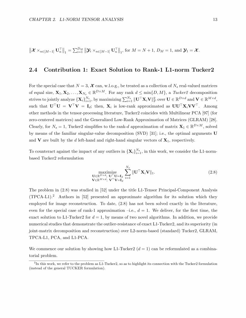
2.4 Contribution 1: Exact Solution to Rank-1 L1-norm Tucker2
For the special case that N = 3, X can, w.l.o.g., be treated as a collection of Ns real-valued matrices
of equal size, X1,X2, . . . ,XNs ∈ RD×M . For any rank d ≤ minD,M, a Tucker2 decomposition
strives to jointly analyze XiNsi=1, by maximizing∑Ns
i=1 ‖U>XiV‖2F over U ∈ RD×d and V ∈ RM×d,such that U>U = V>V = Id; then, Xi is low-rank approximated as UU>XiVV>. Among
other methods in the tensor-processing literature, Tucker2 coincides with Multilinear PCA [97] (for
zero-centered matrices) and the Generalized Low-Rank Approximation of Matrices (GLRAM) [28].
Clearly, for Ns = 1, Tucker2 simplifies to the rank-d approximation of matrix X1 ∈ RD×M , solved
by means of the familiar singular-value decomposition (SVD) [31]; i.e., the optimal arguments U
and V are built by the d left-hand and right-hand singular vectors of X1, respectively.
To counteract against the impact of any outliers in XiNsi=1, in this work, we consider the L1-norm-
based Tucker2 reformulation
maximizeU∈RD×d; U>U=IdV∈RM×d; V>V=Id
Ns∑i=1
‖U>XiV‖1. (2.8)
The problem in (2.8) was studied in [52] under the title L1-Tensor Principal-Component Analysis
(TPCA-L1).2 Authors in [52] presented an approximate algorithm for its solution which they
employed for image reconstruction. To date, (2.8) has not been solved exactly in the literature,
even for the special case of rank-1 approximation –i.e., d = 1. We deliver, for the first time, the
exact solution to L1-Tucker2 for d = 1, by means of two novel algorithms. In addition, we provide
numerical studies that demonstrate the outlier-resistance of exact L1-Tucker2, and its superiority (in
joint-matrix decomposition and reconstruction) over L2-norm-based (standard) Tucker2, GLRAM,
TPCA-L1, PCA, and L1-PCA.
We commence our solution by showing how L1-Tucker2 (d = 1) can be reformulated as a combina-
torial problem.
2In this work, we refer to the problem as L1-Tucker2, so as to highlight its connection with the Tucker2 formulation(instead of the general TUCKER formulation).
CHAPTER 2. L1-NORM TENSOR ANALYSIS 14
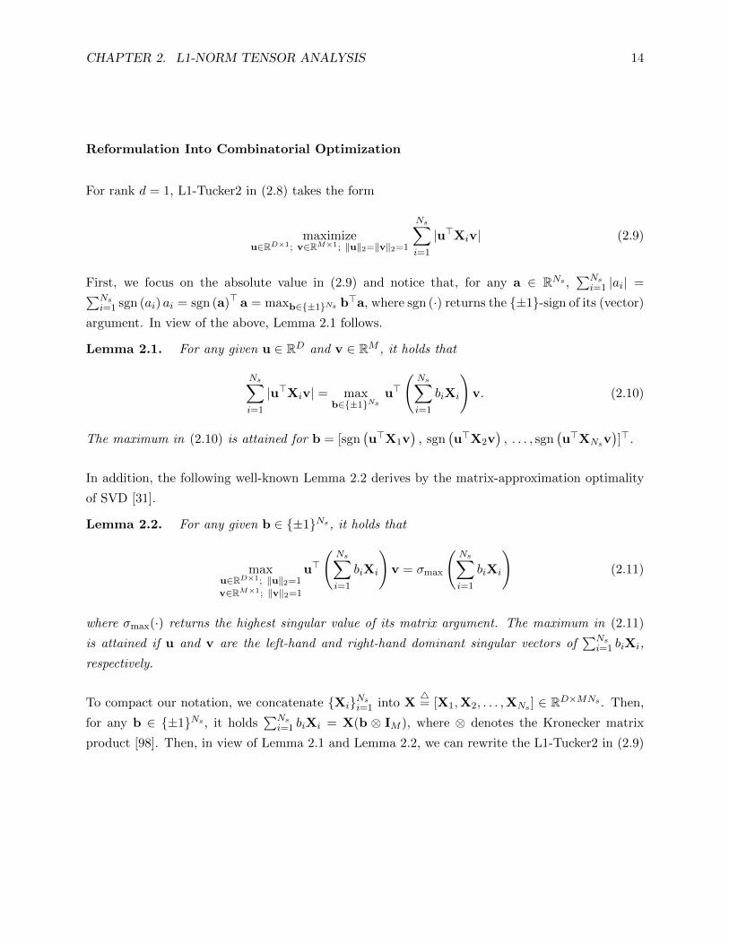
Reformulation Into Combinatorial Optimization
For rank d = 1, L1-Tucker2 in (2.8) takes the form
maximizeu∈RD×1; v∈RM×1; ‖u‖2=‖v‖2=1
Ns∑i=1
|u>Xiv| (2.9)
First, we focus on the absolute value in (2.9) and notice that, for any a ∈ RNs ,∑Ns
i=1 |ai| =∑Nsi=1 sgn (ai) ai = sgn (a)> a = maxb∈±1Ns b>a, where sgn (·) returns the ±1-sign of its (vector)
argument. In view of the above, Lemma 2.1 follows.
Lemma 2.1. For any given u ∈ RD and v ∈ RM , it holds that
Ns∑i=1
|u>Xiv| = maxb∈±1Ns
u>
(Ns∑i=1
biXi
)v. (2.10)
The maximum in (2.10) is attained for b = [sgn(u>X1v
), sgn
(u>X2v
), . . . , sgn
(u>XNsv
)]>.
In addition, the following well-known Lemma 2.2 derives by the matrix-approximation optimality
of SVD [31].
Lemma 2.2. For any given b ∈ ±1Ns, it holds that
maxu∈RD×1; ‖u‖2=1
v∈RM×1; ‖v‖2=1
u>
(Ns∑i=1
biXi
)v = σmax
(Ns∑i=1
biXi
)(2.11)
where σmax(·) returns the highest singular value of its matrix argument. The maximum in (2.11)
is attained if u and v are the left-hand and right-hand dominant singular vectors of∑Ns
i=1 biXi,
respectively.
To compact our notation, we concatenate XiNsi=1 into X4= [X1,X2, . . . ,XNs ] ∈ RD×MNs . Then,
for any b ∈ ±1Ns , it holds∑Ns
i=1 biXi = X(b ⊗ IM ), where ⊗ denotes the Kronecker matrix
product [98]. Then, in view of Lemma 2.1 and Lemma 2.2, we can rewrite the L1-Tucker2 in (2.9)

CHAPTER 2. L1-NORM TENSOR ANALYSIS 15
as
maxu∈RD×1; ‖u‖2=1
v∈RM×1; ‖v‖2=1
Ns∑i=1
|u>Xiv| (2.12)
= maxb∈±1Ns
u∈RD×1; ‖u‖2=1
v∈RM×1; ‖v‖2=1
u> (X(b⊗ IM )) v (2.13)
= maxb∈±1Ns
σmax (X(b⊗ IM )) . (2.14)
It is clear that (2.14) is a combinatorial problem over the size-2Ns feasibility set ±1Ns . The
following Proposition 2.1 derives straightforwardly from Lemma 2.1, Lemma 2.2, and (2.12)-(2.14)
and concludes our transformation of (2.9) into a combinatorial problem.
Proposition 2.1. Let bopt be a solution to the combinatorial
maximizeb∈±Ns
σmax(X(b⊗ IM )) (2.15)
and denote by uopt ∈ RD and vopt ∈ RM the left- and right-hand singular vectors of X(bopt ⊗IM ) ∈ RD×M , respectively. Then, (uopt,vopt) is an optimal solution to (2.9). Also, bopt =
[sgn(u>optX1vopt
), . . . , sgn
(u>optXNsvopt
)]> and
∑Nsi=1 |u>optXivopt| = u>opt(X(bopt ⊗ IM ))vopt =
σmax (X(bopt ⊗ IM )). In the special case that u>optXivopt = 0, for some i ∈ 1, 2, . . . , Ns, [bopt]i
can be set to +1, having no effect to the metric of (2.15).
Given bopt, (uopt,vopt) are obtained by SVD of X(bopt ⊗ IM ). Thus, by Proposition 2.1, the
solution to L1-Tucker2 for low-rank d = 1 is obtained by the solution of the combinatorial problem
(2.15) and a D-by-M SVD.
Connection to L1-PCA and Hardness
In the sequel, we show that for M = 1 and d = 1, L1-Tucker2 in (2.9) simplifies to L1-PCA
[53, 54, 58]. Specifically, for M = 1, matrix Xi is a D × 1 vector, satisfying Xi = xi4= vec(Xi),
and (2.9) can be rewritten as
maxu∈RD; v∈R; ‖u‖2=|v|=1
Ns∑i=1
|u>xiv|. (2.16)
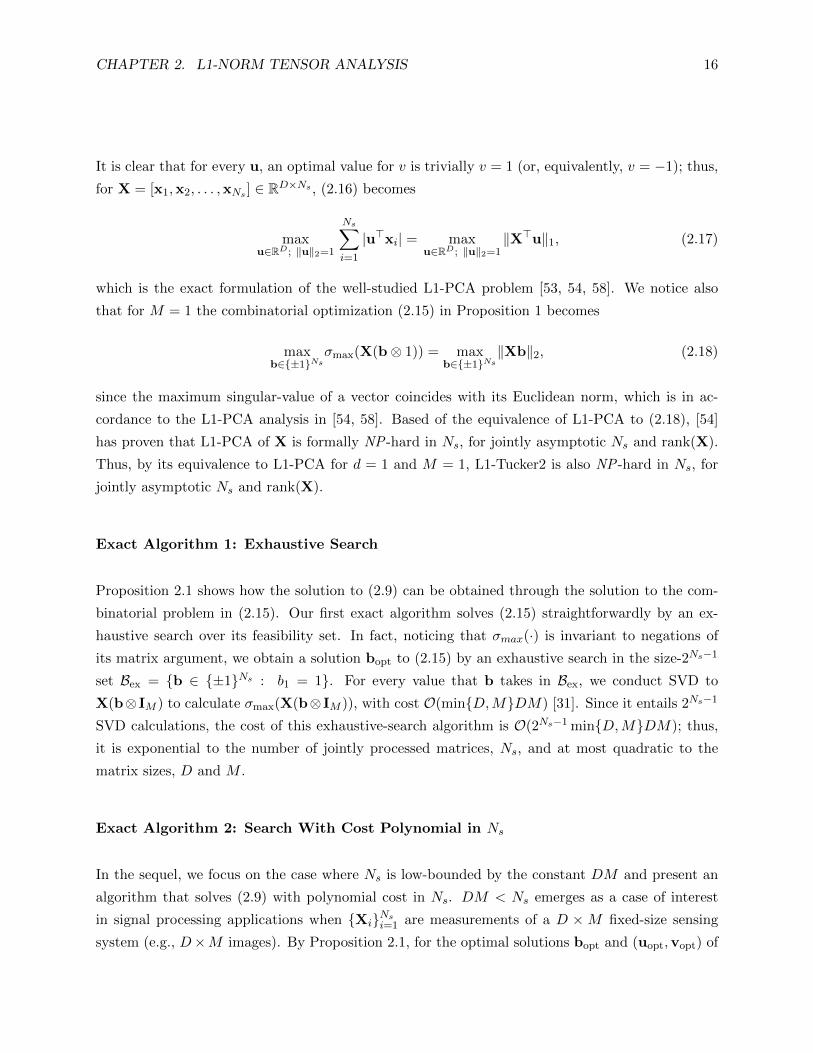
CHAPTER 2. L1-NORM TENSOR ANALYSIS 16
It is clear that for every u, an optimal value for v is trivially v = 1 (or, equivalently, v = −1); thus,
for X = [x1,x2, . . . ,xNs ] ∈ RD×Ns , (2.16) becomes
maxu∈RD; ‖u‖2=1
Ns∑i=1
|u>xi| = maxu∈RD; ‖u‖2=1
‖X>u‖1, (2.17)
which is the exact formulation of the well-studied L1-PCA problem [53, 54, 58]. We notice also
that for M = 1 the combinatorial optimization (2.15) in Proposition 1 becomes
maxb∈±1Ns
σmax(X(b⊗ 1)) = maxb∈±1Ns
‖Xb‖2, (2.18)
since the maximum singular-value of a vector coincides with its Euclidean norm, which is in ac-
cordance to the L1-PCA analysis in [54, 58]. Based of the equivalence of L1-PCA to (2.18), [54]
has proven that L1-PCA of X is formally NP -hard in Ns, for jointly asymptotic Ns and rank(X).
Thus, by its equivalence to L1-PCA for d = 1 and M = 1, L1-Tucker2 is also NP -hard in Ns, for
jointly asymptotic Ns and rank(X).
Exact Algorithm 1: Exhaustive Search
Proposition 2.1 shows how the solution to (2.9) can be obtained through the solution to the com-
binatorial problem in (2.15). Our first exact algorithm solves (2.15) straightforwardly by an ex-
haustive search over its feasibility set. In fact, noticing that σmax(·) is invariant to negations of
its matrix argument, we obtain a solution bopt to (2.15) by an exhaustive search in the size-2Ns−1
set Bex = b ∈ ±1Ns : b1 = 1. For every value that b takes in Bex, we conduct SVD to
X(b⊗ IM ) to calculate σmax(X(b⊗ IM )), with cost O(minD,MDM) [31]. Since it entails 2Ns−1
SVD calculations, the cost of this exhaustive-search algorithm is O(2Ns−1 minD,MDM); thus,
it is exponential to the number of jointly processed matrices, Ns, and at most quadratic to the
matrix sizes, D and M .
Exact Algorithm 2: Search With Cost Polynomial in Ns
In the sequel, we focus on the case where Ns is low-bounded by the constant DM and present an
algorithm that solves (2.9) with polynomial cost in Ns. DM < Ns emerges as a case of interest
in signal processing applications when XiNsi=1 are measurements of a D ×M fixed-size sensing
system (e.g., D×M images). By Proposition 2.1, for the optimal solutions bopt and (uopt,vopt) of

CHAPTER 2. L1-NORM TENSOR ANALYSIS 17
(2.15) and (2.9), respectively, it holds
bopt = [sgn(v>optX
>1 uopt
), . . . , sgn
(v>optX
>Nsuopt
)]>, (2.19)
with sgn(u>optXivopt
)= +1, if u>optXivopt = 0. In addition, for every i ∈ 1, 2, . . . , Ns, we find
that
v>optX>i uopt = Tr
(X>i uoptv
>opt
)= x>i (vopt ⊗ uopt). (2.20)
Therefore, defining Y = [x1,x2, . . . ,xNs ] ∈ RDM×Ns , (2.19) can be rewritten as
bopt = sgn(Y>(vopt ⊗ uopt)
). (2.21)
Consider now that Y is of some rank ρ ≤ minDM,Ns and admits SVD Ysvd= QSW, where
Q>Q = WW> = Iρ and S is the ρ× ρ diagonal matrix that carries the ρ non-zero singular-values
of Y. Defining popt4= S>Q>(vopt ⊗ uopt), (2.21) can be rewritten as
bopt = sgn(W>popt
). (2.22)
In view of (2.22) and since sgn (·) is invariant to positive scalings of its vector argument, an optimal
solution to (2.15), bopt, can be found in the binary set
B = b ∈ ±1Ns : b = sgn(W>c
), c ∈ Rρ. (2.23)
Certainly, by definition, (2.23) is a subset of ±1Ns and, thus, has finite size upper bounded by 2Ns .
This, in turn, implies that there exist instances of c ∈ Rρ that yield the same value in sgn(W>c
).
Below, we delve into this observation to build a tight superset of B that has polynomial size in Ns,
under the following mild “general position” assumption [99].
Assumption 2.1. For every I ⊂ 1, 2, . . . , Ns with |I| = ρ−1, it holds that rank([W]:,I) = ρ−1;
i.e., any collection of ρ− 1 columns of W are linearly independent.
For any i ∈ 1, 2, . . . , Ns, define wi4= [W]:,i and denote by Ni the nullspace of wi. Then, for every
c ∈ Ni, the (non-negative) angle between c and wi, φ(c,wi), is equal to π2 and, accordingly, w>i c =
‖c‖2‖wi‖2 cos (φ(c,wi)) = 0. Clearly, the hyperplane Ni partitions Rρ in two non-overlapping
halfspaces, H+i and H−i [100], such that sgn
(c>wi
)= +1 for every c ∈ H+
i and sgn(c>wi
)= −1
for every c ∈ H−i . In accordance with Proposition 2.1, we consider that H+i is a closed set that
includes its boundary Ni, whereas H−i is open and does not overlap with Ni. In view of these

CHAPTER 2. L1-NORM TENSOR ANALYSIS 18
Figure 2.3. For ρ = 3 and Ns = 4, we draw W ∈ Rρ×N , such that WW> = I3 and Assumption 1holds true. Then, we plot the nullspaces of all 4 columns of W (colored planes). We observe thatthe planes partition R3 into K = 2(
(30
)+(
31
)+(
32
)) = 2(1 + 3 + 3) = 14 coherent cells (i.e., 7 visible
cells above the cyan hyperplane and 7 cells below.)
definitions, we proceed with the following illustrative example.
Consider some ρ > 2 and two column indices m < i ∈ 1, 2, . . . , Ns. Then, hyperplanes Nm and
Ni divide Rρ in the halfspace pairs H+m,H−m and H+
i ,H−i , respectively. By Assumption 2.1,3
each one of the two halfspaces defined by Nm will intersect with both halfspaces defined by Ni,forming the four halfspace-intersection “cells” C1 = H+
m ∩ H+i , C2 = H+
m ∩ H−i , C3 = H−m ∩ H−i ,
C4 = H−m ∩H+i . It is now clear that, for any k ∈ 1, 2, 3, 4, [sgn
([W]>c
)]m,i is the same for every
c ∈ Ck. For example, for every c ∈ C2, it holds that [sgn([W]>c
)]m = +1 and [sgn
([W]>c
)]i = −1.
Next, we go one step further and consider the arrangement of all N hyperplanes NiNsi=1. Similar
to our discussion above, these hyperplanes partition Rρ in K cells CkKk=1, where K depends on ρ
and Ns. Formally, for every k, the k-th halfspace-intersection set is defined as
Ck4=⋂i∈I+k
H+i
⋂m∈I−1
k
H−m, (2.24)
3If wm and wi are linearly independent, then Nm and Ni intersect but do not coincide.

CHAPTER 2. L1-NORM TENSOR ANALYSIS 19
for complementary index sets I+k and I−k that satisfy I+
k ∩ I−k = ∅ and I+
k ∪ I−k = 1, 2, . . . , Ns
[101, 102]. By the definition in (2.24), and in accordance with our example above, every c ∈ Cklies in the same intersection of halfpsaces and, thus, yields the exact same value in sgn
(W>c
).
Specifically, for every c ∈ Ck, it holds that
[sgn
(W>c
)]i
= sgn(w>i c
)=
+1, i ∈ I+
k
−1, i ∈ I−k. (2.25)
In view of (2.25), for every k ∈ 1, 2, . . . ,K and any c ∈ Ck, we define the “signature” of the k-th
cell bk4= sgn
(W>c
). Moreover, we observe that Ck ∩Cl = ∅ for every k 6= l and that ∪Kk=1Ck = Rρ.
By the above observations and definitions, (2.23) can be rewritten as
B =K⋃k=1
sgn(W>c
): c ∈ Ck = b1,b2, . . . ,bK. (2.26)
Importantly, in [101, 103], it was shown that the exact number of coherent cells formed by the
nullspaces of Ns points in Rρ that are in general position (under Assumption 2.1) is exactly
K = 2
ρ−1∑j=0
(Ns − 1
j
)≤ 2Ns , (2.27)
with equality in (2.27) if and only if ρ = Ns. Accordingly, per (2.27), the cardinality of B in (2.23)
is equal to |B| = 2∑ρ−1
j=0
(Ns−1j
). For clarity, in Fig. 2.3, we plot the nullspaces (colored planes)
of the columns of arbitrary W ∈ R3×4 that satisfies both WW> = I3 and Assumption 2.1. It is
interesting that exactly K = 14 < 24 = 16 coherent cells emerge by the intersection of the formed
halfspaces. In the sequel, we rely on (2.26) to develop a conceptually simple method for computing
a tight superset of the cell signatures in B.
Under Assumption 2.1, for any I ⊆ 1, 2, . . . , Ns with |I| = ρ − 1, the hyperplane intersection
VI4= ∩i∈INi is a line (1-dimensional subspace) in Rρ. By its definition, this line is the verge
between all cells that are jointly bounded by the ρ − 1 hyperplanes in Nii∈I . Consider now a
vector c ∈ Rρ that crosses over the verge VI (at any point other than 0ρ). By this crossing, the
value of [sgn(W>c
)]I will change so that sgn
(W>c
)adjusts to the signature of the new cell to
which c just entered. At the same time, a crossing over VI cannot be simultaneously over any of
the hyperplanes in Nii∈Ic , for Ic 4= 1, 2, . . . , Ns\I; this is because, under Assumption 2.1, it is
only at 0ρ that more than ρ−1 hyperplanes can intersect. Therefore, it is clear that [sgn(W>c
)]Ic
will remain invariant during this crossing and, in fact, equal to [sgn(W>v
)]Ic , for any v ∈ VI with
CHAPTER 2. L1-NORM TENSOR ANALYSIS 20
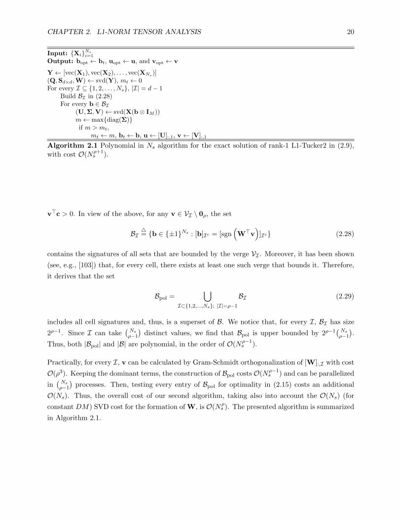
Input: XiNsi=1
Output: bopt ← bt, uopt ← u, and vopt ← v
Y ← [vec(X1), vec(X2), . . . , vec(XNs)](Q,Sd×d,W)← svd(Y), mt ← 0For every I ⊆ 1, 2, . . . , Ns, |I| = d− 1
Build BI in (2.28)For every b ∈ BI
(U,Σ,V)← svd(X(b⊗ IM ))m← maxdiag(Σ)if m > mt,
mt ← m, bt ← b, u← [U]:,1, v← [V]:,1
Algorithm 2.1 Polynomial in Ns algorithm for the exact solution of rank-1 L1-Tucker2 in (2.9),with cost O(Nρ+1
s ).
v>c > 0. In view of the above, for any v ∈ VI \ 0ρ, the set
BI4= b ∈ ±1Ns : [b]Ic = [sgn
(W>v
)]Ic (2.28)
contains the signatures of all sets that are bounded by the verge VI . Moreover, it has been shown
(see, e.g., [103]) that, for every cell, there exists at least one such verge that bounds it. Therefore,
it derives that the set
Bpol =⋃
I⊂1,2,...,Ns; |I|=ρ−1
BI (2.29)
includes all cell signatures and, thus, is a superset of B. We notice that, for every I, BI has size
2ρ−1. Since I can take(Nsρ−1
)distinct values, we find that Bpol is upper bounded by 2ρ−1
(Nsρ−1
).
Thus, both |Bpol| and |B| are polynomial, in the order of O(Nρ−1s ).
Practically, for every I, v can be calculated by Gram-Schmidt orthogonalization of [W]:,I with cost
O(ρ3). Keeping the dominant terms, the construction of Bpol costs O(Nρ−1s ) and can be parallelized
in(Nsρ−1
)processes. Then, testing every entry of Bpol for optimality in (2.15) costs an additional
O(Ns). Thus, the overall cost of our second algorithm, taking also into account the O(Ns) (for
constant DM) SVD cost for the formation of W, is O(Nρs ). The presented algorithm is summarized
in Algorithm 2.1.

CHAPTER 2. L1-NORM TENSOR ANALYSIS 21
6 8 10 12 14 16 18 20 220
2000
4000
6000
8000
10000
12000
14000
Figure 2.5. Reconstruction MSE versus corruption variance σ2c (dB).
2.4.1 Numerical Studies
Consider Xi14i=1 such that Xi = Ai + Ni ∈ R20×20 where Ai = biuv> and ‖u‖2 = ‖v‖2 = 1,
bi ∼ N (0, 49), and each entry of Ni is additive white Gaussian noise (AWGN) from N (0, 1). We
consider that Ai is the rank-1 useful data in Xi that we want to reconstruct, by joint analysis
(Tucker2-type) of Xi14i=1. By irregular corruption, 30 entries in 2 out of the 14 matrices (i.e., 60
entries out of the total 5600 entries in Xi14i=1) have been further corrupted additively by noise
from N (0, σ2c ). To reconstruct Ai14
i=1 from Xi14i=1, we follow one of the two approaches below.
In the first approach, we vectorize the matrix samples and perform standard matrix analysis. That
is, we obtain the first (d = 1) principal component (PC) of [vec(X1), vec(X2), . . . , vec(XNs)], q.
Then, for every i, we approximate Ai by Ai = mat(qq>ai), where mat(·) reshapes its vector
argument into a 20 × 20 matrix, in accordance with vec(·). In the second approach, we process
the samples in their natural form, as matrices, analyzing them by Tucker2. If (u,v) is the Tucker2
solution pair, then we approximate Ai by Ai = uu>Xivv>. For the first approach, we obtain q
by PCA (i.e., SVD) and L1-PCA [54]. For the second approach, we conduct Tucker2 by HOSVD
[17], HOOI [32], GLRAM [28], TPCA-L1 [52], and the proposed exact L1-Tucker2. Then, for
each reconstruction method, we measure the mean of the squared error∑14
i=1 ‖Ai − Ai‖2F over
1000 independent realizations for corruption variance σ2c = 6, 8, . . . , 22dB. In Fig. 2.5, we plot the
reconstruction mean squared error (MSE) for every method, versus σ2c . We observe that PCA and
L1-PCA exhibit the highest MSE due to the vectorization operation (L1-PCA outperforms PCA
clearly, across all values of σ2c ). Then, all Tucker2-type methods perform similarly well when σ2
c
CHAPTER 2. L1-NORM TENSOR ANALYSIS 22
is low. As the outlier variance σ2c increases, the performance of L2-norm-based Tucker2 (HOSVD,
HOOI) and GLRAM deteriorates severely. On the other hand, the L1-norm-based TPCA-L1
exhibits some robustness. The proposed exact L1-Tucker2 maintains the sturdiest resistance against
the corruption, outperforming its counterparts across the board.
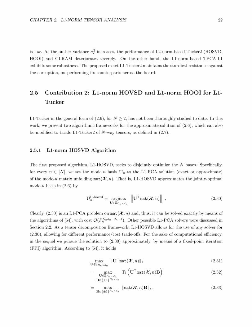
2.5 Contribution 2: L1-norm HOVSD and L1-norm HOOI for L1-
Tucker
L1-Tucker in the general form of (2.6), for N ≥ 2, has not been thoroughly studied to date. In this
work, we present two algorithmic frameworks for the approximate solution of (2.6), which can also
be modified to tackle L1-Tucker2 of N -way tensors, as defined in (2.7).
2.5.1 L1-norm HOSVD Algorithm
The first proposed algorithm, L1-HOSVD, seeks to disjointly optimize the N bases. Specifically,
for every n ∈ [N ], we set the mode-n basis Un to the L1-PCA solution (exact or approximate)
of the mode-n matrix unfolding mat(X , n). That is, L1-HOSVD approximates the jointly-optimal
mode-n basis in (2.6) by
Ul1-hosvdn = argmax
U∈SDn×dn
∥∥∥U>mat(X , n)∥∥∥
1. (2.30)
Clearly, (2.30) is an L1-PCA problem on mat(X , n) and, thus, it can be solved exactly by means of
the algorithms of [54], with cost O(PDndn−dn+1n ). Other possible L1-PCA solvers were discussed in
Section 2.2. As a tensor decomposition framework, L1-HOSVD allows for the use of any solver for
(2.30), allowing for different performance/cost trade-offs. For the sake of computational efficiency,
in the sequel we pursue the solution to (2.30) approximately, by means of a fixed-point iteration
(FPI) algorithm. According to [54], it holds
maxU∈SDn×dn
‖U>mat(X , n)‖1 (2.31)
= maxU∈SDn×dn
B∈±1Pn×dn
Tr(U>mat(X , n)B
)(2.32)
= maxB∈±1Pn×dn
‖mat(X , n)B‖∗. (2.33)

CHAPTER 2. L1-NORM TENSOR ANALYSIS 23
Input: X ∈ RD1×...×DN , dnn∈[N ]
Output: Unn∈[N ]
Initialize Unn∈[N ] by HOSVD of X for dnn∈[N ]
For n = 1, 2, . . . , NUntil convergence/termination
Un ← Φ(mat(X , n)sgn(mat(X , n)>Un)
)Algorithm 2.2 L1-HOSVD algorithm for L1-Tucker (L1HOSVD(X , dnn∈[N ])).
For fixed B, (2.32) is maximized by U = Φ(mat(X , n)B). At the same time, for fixed U, (2.32)
is maximized by B = sgn(mat(X , n)>U). Accordingly, a solution to (2.30) can be pursued in
an alternating fashion, as Bt = sgn(mat(X , n)>Ut−1) = argmaxB∈±1Pn×dnTr(U>t−1mat(X , n)B
)and Ut = Φ(mat(X , n)Bt)=argmaxU∈SDn×dn Tr
(U>mat(X , n)Bt
), for t = 1, 2, . . ., and arbitrary
initialization U0 ∈ SDn×dn . Interestingly, the alternating optimization above, can be rewritten in
the compact FPI form
Ut = Φ(mat(X , n)sgn(mat(X , n)>Ut−1)
). (2.34)
A proof of convergence for the recursion in (2.34) is offered in the Appendix A. If Tn is the index
of the converging iteration, then Ul1-hosvdn is approximated by UTn . Similarly, the N − 1 first bases
Ul1-hosvdn N−1
n=1 can be used as an approximate solution to L1-Tucker2 in (2.7).
Complexity of L1-HOSVD
For any given t and n, the computational cost of (2.34) is O(dnP ), where P4=∏m∈[N ]Dm. In
practice, we have observed that, for any n, it suffices to terminate iterations at a linear multiple of
Dn. Thus, for any n, Ul1-hosvdn is approximated with cost O(DndnP ). Accordingly, the total cost
of L1-HOSVD is O(maxn∈[N ] dnDnP ). Considering, for simplicity in presentation, that Dn = D
and dn = d for every n, then the complexity of L1-HOSVD can be rewritten as O(dDN+1).
A pseudocode of L1-HOSVD is offered in Algorithm 2.2.

CHAPTER 2. L1-NORM TENSOR ANALYSIS 24
Input: X ∈ RD1×...×DN , dnn∈[N ]
Output: Unn∈[N ]
Initialize Unn∈[N ]
Until termination/convergenceFor n = 1, 2, . . . , N
A← mat(X ×m<n Um
> ×k>n Uk>, n
)Until termination/convergence
Un ← Φ(Asgn(A>Un))
Algorithm 2.3 L1-HOOI algorithm for L1-Tucker (L1HOOI(X , dnn∈[N ]))
2.5.2 L1-norm HOOI Algorithm
Next, we present L1-HOOI, an alternative method for jointly optimizing the L1-Tucker bases. First,
L1-HOOI is initialized to N feasible bases (e.g., those returned by L1-HOSVD). Then, it conducts
a sequence of iterations across which it updates all bases such that the objective value of L1-Tucker
increases. Thus, when initialized to the L1-HOSVD bases, L1-HOOI is guaranteed to outperform
L1-HOSVD in the L1-Tucker metric. A detailed description of L1-HOOI follows.
First, we initialize U(0)n ∈ SDn×dnn∈[N ]; for instance, one can set U
(0)n = Ul1-hosvd
n . Then, at the
q-th iteration, q = 1, 2, . . ., all N bases are successively optimized in order of increasing mode-index
n = 1, 2, . . . , N . Specifically, at a given iteration q and mode index n, we fix U(q)m for m < n and
U(q−1)k for k > n and seek the mode-n basis U
(q)n that maximizes the L1-Tucker metric. That is,
for given (q, n), we update
U(q)n = argmax
U∈SDn×dn
∥∥∥U>A(q)n
∥∥∥1, (2.35)
where A(q)n4= mat
(X ×m<n U
(q)m
>×k>n U
(q−1)k
>, n
)∈ RDn×pn and pn
4=∏i∈[N ]\n di for every n.
We notice that, in contrast to (2.30), the metric of (2.35) involves the jointly optimized bases of
the other modes. Similar to L1-HOSVD, an array of L1-PCA solvers, as discussed in Section 2.2,
can be used for solving (2.35), attaining different performance/cost trade-offs. For simplicity in
presentation, here we employ the FPI in (2.34). That is, for any (q, n), we set U(q)n to the converging
argument of the sequence
Ut = Φ(A(q)n sgn(A(q)
n
>Ut−1)
), (2.36)
where for every n, U0 = U(q−1)n . A pseudocode of the proposed L1-HOOI method is offered in

CHAPTER 2. L1-NORM TENSOR ANALYSIS 25
Algorithm 2.3. Similar to L1-HOSVD, L1-HOOI can be used for the approximate solution of L1-
Tucker2 simply by fixing U(q)N to IDN for every q. A convergence analysis of the L1-HOOI iterations
is presented below.
Convergence of L1-HOOI
We commence our convergence analysis with Lemma 2.3, which shows that the q-th update of the
mode-n basis increases the L1-Tucker metric.
Lemma 2.3. For given U(q)m m<n and U(q−1)
k k>n (and, thus, given A(q)n ), it holds that∥∥∥U(q)
n
>A(q)n
∥∥∥1≥∥∥∥U(q−1)
n
>A(q)n
∥∥∥1. (2.37)
Lemma 2.3 derives straightforwardly from the convergence proof of (2.34), presented in the Ap-
pendix. Moreover, we note that Lemma 2.3 would also hold if, instead of the FPI of (2.34), we
solved (2.35) by means of the bit-flipping algorithm of [58]. Also, Lemma 2.3 holds true if U(q)n is
computed by the exact solution of (2.35) obtained by the algorithms of [54]. The following Lemma
2.4 shows that, within the same iteration, the metric increases as we successively optimize the
bases.
Lemma 2.4. For any q > 0 and every n > m ∈ [N ], it holds that
∥∥∥∥U(q)n
>A
(q)n
∥∥∥∥1
≥∥∥∥∥U(q)
m
>A
(q)m
∥∥∥∥1
and
∥∥∥∥U(q)1
>A
(q)1
∥∥∥∥1
≥∥∥∥∥U(q−1)
N
>A
(q−1)N
∥∥∥∥1
.
In view of Lemma 2.4, the following Proposition 2.2 holds true and summarizes the L1-Tucker
metric increase across the L1-HOOI iterations.
Proposition 2.2. For any n ∈ [N ] and every q′ > q∥∥∥U(q′)n
>A(q′)n
∥∥∥1≥∥∥∥U(q)
n
>A(q)n
∥∥∥1. (2.38)
Defining p4=∏n∈[N ] dn, the following Lemma 2.5 provides an upper bound for the L1-Tucker
metric.

CHAPTER 2. L1-NORM TENSOR ANALYSIS 26
1 2 3 4 5 6 7 8 9 10 11 12 13 14 15 16
Iteration index q
8.6
8.8
9
9.2
9.4
9.6
9.8
10
L1-T
ucker
metr
ic
L1-HOOIL1-HOSVD iniatialization
Figure 2.8. L1-Tucker metric across L1-HOOI iterations.
Lemma 2.5. For any Un ∈ SDn×dnn∈[N ], it holds that
‖X ×n∈[N ] U>n ‖1 ≤√p‖X‖F . (2.39)
Lemma 2.5 shows that the L1-Tucker metric is upper bounded by√p‖X‖F . This, in conjunc-
tion with Proposition 2.2, implies that as q increases the L1-HOOI iterations converge in the
L1-Tucker metric. To visualize the convergence, we carry out the following study. We form 5-
way tensor X ∈ R10×10×...×10 that draws entries independently from N (0, 1). Then, we apply
to it L1-HOOI initialized at L1-HOSVD. In Fig. 2.8, we plot the evolution of the L1-Tucker
metric ‖X ×n∈[N ] U(q)n
>‖1, versus the L1-HOOI iteration index q. In accordance to our for-
mal analysis, we observe the monotonic increase of the metric and convergence after just 16
iterations. In practice, one can terminate the L1-HOOI iterations when the metric-increase ra-
tio ζ(q)4=
∥∥∥∥X ×n∈[N ] U(q)n
>∥∥∥∥
1
∥∥∥∥X ×n∈[N ] U(q−1)n
>∥∥∥∥
1
−1
− 1 drops below a predetermined threshold
τ > 0, or when q exceeds a maximum number of permitted iterations.
Next, we discuss the computational cost of L1-HOOI.
CHAPTER 2. L1-NORM TENSOR ANALYSIS 27
Complexity of L1-HOOI
For simplicity in presentation, we consider again Di = D and di = d, for every i ∈ [N ]. As shown
above, initialization of L1-HOOI by means of L1-HOSVD costs O(dDN+1). Then, at iteration q,
L1-HOOI computes matrix A(q)n in (2.35) and its L1-PCA, for every n. Matrix A
(q)n can computed
by a sequence of matrix-to-matrix products as follows. First, we compute the mode-k product of
X with U(zk)k , for some k 6= n (zk = q if k < n and zk = q − 1 if k > n), with cost O(dDN ).
Next, we compute the l-mode product of X ×k U(zk)k with U
(zl)l , for some l /∈ n, k, with cost
O(d2DN−1). We observe that the second product (l-mode) has lower cost than the first one (k-
mode), for any selection of k and l. Similarly, each subsequent mode product will have further
reduced cost. Keeping as dominant term the cost of the first product, the computation of A(q)n
costs O(dDN ). After A(q)n ∈ RD×dN−1
is computed, the solution to (2.35) is approximated by
fixed point iterations with cost O(D2dN ). Thus, the cost of a single iteration of L1-HOOI is
O(dDN +D2dN ). Denoting by T the maximum number of iterations permitted, the overall cost of
L1-HOOI is O(T (dDN + D2dN )), comparable to the costs of standard HOSVD and HOOI which
are O(DN+1) and O(TdDN ), respectively. These computational costs are summarized in Table
2.1.
2.5.3 Numerical Studies
Tensor Reconstruction
We set N = 5, D1 = D3 = D5 = 10, D2 = D4 = 15, d1 = d2 = 6, d3 = d4 = d5 = 4, and generate
Tucker-structured X = G ×n∈[5] Un. The core tensor G draws entries from N (0, 9) and, for every
n, Un is an arbitrary orthonormal basis. Then, we corrupt all entries of X with zero-mean unit-
variance additive white Gaussian noise (AWGN), disrupting its Tucker structure. Moreover, we
corrupt No out of the 225, 000 entries of X by adding high-variance outliers from N (0, σ2o). Thus,
we form X corr = X +N +O, where N and O model AWGN and sparse outliers, respectively. Our
objective is to reconstruct X from the available X corr. For that purpose, we Tucker decompose
X corr by means of HOSVD, HOOI, L1-HOSVD, and L1-HOOI and obtain bases Unn∈[5]. Then,
we reconstruct X as X = X corr ×n∈[5] UnU>n . The normalized squared error (NSE) is defined as
‖X − X‖2F ‖X‖−2F . In Fig. 2.9a, we set No = 300 and plot the mean NSE (MNSE), evaluated over
1000 independent noise/outlier realizations, versus outlier standard deviation σo = 4, 8, . . . , 28. In
the absence of outliers (σo = 0), all methods under comparison exhibit similarly low MNSE. As
the outlier standard deviation σo increases the MNSE of all methods increases. We notice that the

CHAPTER 2. L1-NORM TENSOR ANALYSIS 28
Table 2.1: Computational costs of PCA, L1PCA-FPI, HOSVD, L1-HOSVD (proposed), HOOI,and L1-HOOI (proposed). PCA/L1PCA-FPI costs are reported for input matrix X ∈ RD×Dand decomposition rank d. Tucker/L1-Tucker costs are reported for N -way input tensor X ∈RD×D×...×D and mode-n ranks dn = d ∀n. T is the maximum number of iterations conducted byHOOI and L1-HOOI.
Method Cost
PCA (SVD) O(D3)
L1-PCA (FPI) O(D2d
)HOSVD O
(DN+1
)L1-HOSVD O
(dDN+1
)HOOI O
(TdDN
)L1-HOOI O
(T (dDN +D2dN )
)
performances of HOSVD and HOOI markedly deteriorate for σo ≥ 12 and σo ≥ 20 respectively.
On the other hand, L1-HOSVD and L1-HOOI remain robust against corruption, across the board.
In Fig. 2.9b, we set σo = 26 and plot the MNSE versus number of outliers No = 0, 40, . . . , 400.
Expectedly, in the absence of outliers (No = 0), all methods exhibit low MNSE. As the number of
outliers increases, HOSVD and HOOI start exhibiting high reconstruction error, while L1-HOSVD
and L1-HOOI remain robust. For instance, the MNSE of L1-HOSVD for No = 400 outliers is lower
than the MNSE of standard HOSVD for No = 40 (ten times fewer) outliers.
Finally, in Fig. 2.9c, we set σo = 28, No = 150 (≈ 0.07% of total data entries are corrupted)
and plot the MNSE versus dn∀n while dm is set to its nominal value for every m ∈ [N = 5] \ n.
We observe that, even for a very small fraction of outlier corrupted entries in X corr, standard
Tucker methods are clearly misled across all 5 modes. On the other hand, the proposed L1-Tucker
counterparts, exhibit sturdy outlier resistance and reconstruct X well, remaining almost unaffected
by the outlying entries in X corr.
A robust tensor analysis algorithm, specifically designed for counteracting sparse outliers, is the
High-Order Robust PCA (HORPCA) [50]. Formally, given X corr, HORPCA solves
min.X ,O∈RD1×...×DN
∑Nn=1 ‖mat
(X , n
)‖∗ + λ‖O‖1
subject to X + O = X corr. (2.40)
Authors in [50] presented the HoRPCA-S algorithm for the solution of (2.40) which relies on a
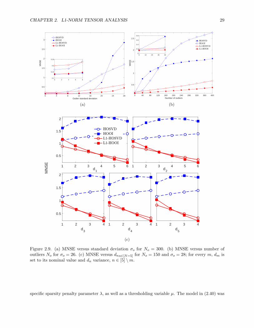
CHAPTER 2. L1-NORM TENSOR ANALYSIS 29
0 4 8 12 16 20 24 28Outlier standard deviation
0.5
1
1.5
2
2.5
3M
NS
E
0 2 4 6 80.1
0.15
0.2
0.25
(a)
0 40 80 120 160 200 240 280 320 360 400Number of outliers
0.5
1
1.5
2
2.5
MN
SE
0 10 20 30 400
0.2
0.4
0.6
0.8
(b)
1 2 3 4 5 6d
1
0.5
1
1.5
2
MN
SE
1 2 3 4 5 6d
2
1 2 3 4d
3
0.5
1
1.5
2
1 2 3 4d
4
1 2 3 4d
5
(c)
Figure 2.9. (a) MNSE versus standard deviation σo for No = 300. (b) MNSE versus number ofoutliers No for σo = 26. (c) MNSE versus dnn∈[N=5] for No = 150 and σo = 28; for every m, dm isset to its nominal value and dn variance, n ∈ [5] \m.
specific sparsity penalty parameter λ, as well as a thresholding variable µ. The model in (2.40) was

CHAPTER 2. L1-NORM TENSOR ANALYSIS 30
0.5 1 1.5 2 2.5 30
0.2
0.4
0.6
0.8
1
MN
SE
HORPCA, =300HORPCA, =500HORPCA+HOSVD, =300HORPCA+HOSVD, =500Benchmark (noise-to-data)HOOIL1-HOOI
Figure 2.10. MNSE versus λ for varying µ.
introduced considering that, apart from the sparse outliers, there is no dense (full rank) corruption
to X (see [50], subsection 2.6). In the case of additional dense corruption, HORPCA is typically
refined by HOSVD [50, 70, 71]. In the sequel, we refer to this approach as HORPCA+HOSVD.
In our next study, we set N = 5, Dn = 5, and dn = 2 for every n, and build the Tucker-structured
data tensor X = G×n∈[5] Un, where the entries of core G are independently drawn from N (0, 122).
Then, we add both dense AWGN and sparse outliers, creating X corr = X+N+O, where the entries
of noise N are drawn independently from N (0, 1) and the 15 non-zero entries of O (in arbitrary
locations) are drawn from N (0, 202). Then, we attempt to reconstruct X from the available X corr
using HOOI, HORPCA (for λ = 0.2, 0.6, . . . , 3 and µ = 300, 500), HORPCA+HOSVD (same λ and
µ combinations as HORPCA), and the proposed L1-HOOI.
In Fig. 2.10, we plot MNSE computed over 50 data/noise/corruption realizations, versus λ for
the four methods. In addition, we plot the average noise-to-data benchmark ‖N ‖2F ‖X‖−2F . In ac-
cordance with our previous studies, we observe that L1-HOOI offers markedly lower MNSE than
standard HOOI. In addition, we notice that for specific selection of µ and λ (µ = 300 and λ = 0.6)
HORPCA+HOSVD attains MNSE slightly lower than L1-HOOI. However, for any different selec-
tion of λ L1-HOOI attains markedly better reconstruction. In addition, we plot the performance of
HORPCA when it is not refined by HOSVD. We notice that, expectedly, for specific selections of µ
and λ the method is capable of removing the outliers, but not the dense noise component –thus, the
MNSE approaches the average noise-to-data benchmark. This study corroborates the corruption-
resistance of L1-HOOI, while, similar to HOOI, it does not depend on any tunable parameters,
other than dnn∈[N ].

CHAPTER 2. L1-NORM TENSOR ANALYSIS 31
Classification
Tucker decomposition is commonly employed for classification of multi-way data samples. Below,
we consider the Tucker-based classification framework originally presented in [104]. That is, we
consider C classes of order-N tensor objects of size D1 ×D2 × . . . ×DN and Mc labeled samples
available from the c-th class, c ∈ [C], that can be used for training a classifier. The training data
from class c are organized in tensor Xc ∈ RD1×D2×...×DN×Mc and the total of M =∑C
c=1Mc training
data are organized in tensor X ∈ RD1×...×DN×M , constructed by concatenation of X1, . . . ,XC across
mode (N + 1).
In the first processing step, X is Tucker decomposed, obtaining feature bases Un ∈ SDn×dnn∈[N ]
for the first N modes (feature modes) and the sample basis Q ∈ SM×M for the (N + 1)-th mode
(sample mode). The obtained feature bases are then used to compress the training data, as
Gc = Xc ×n∈[N ] U>n ∈ Rd1×...×dN×Mc (2.41)
for every c ∈ [C]. Then, the Mc compressed tensor objects from the c-th class are vectorized
(equivalent to mode-(N + 1) flattening) and stored in the data matrix
Gc = mat (Gc, N + 1)> ∈ Rp×Mc , (2.42)
where p =∏n∈[N ] dn. Finally, the labeled columns of Gcc∈[C] are used to train any standard
vector-based classifier, such as support vector machines (SVM), or k-nearest-neighbors (k-NN).
When an unlabeled testing point Y ∈ RD1×...×DN is received, it is first compressed using the
Tucker-trained bases as Z = Y×n∈[N ]U>n . Then, Z is vectorized as z = vec(Z) = mat (Z, N + 1)>.
Finally, vector z is classified based on the standard vector classifier trained above.
In this study, we focus on the classification of order-2 data (N = 2) from the MNIST image dataset
of handwritten digits [105]. Specifically, we consider C = 5 digit classes (digits 0, 1, . . . , 4) and
M1 = . . . = M5 = 10 image samples of size (D = D1 = 28) × (D = D2) available from each class.
To make the classification task more challenging, we consider that each training image is corrupted
by heavy-tail noise with probability α. Then, each pixel of a corrupted image is additively corrupted
by a noise component w ∼ unif(0, v), with probability β. Denoting the average pixel energy by
E = 1D2M‖X‖2F , we choose v so that
√E
Ew2 = 10. We conduct Tucker-based classification as
described above, for d = d1 = d2, using a nearest-neighbor (NN) classifier (i.e., 1-NN), by which
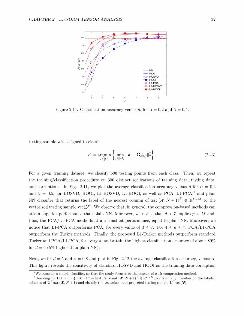
CHAPTER 2. L1-NORM TENSOR ANALYSIS 32
3 4 5 6 7 8 9
0.5
0.55
0.6
0.65
0.7
0.75
0.8
0.85
Accuracy
NNPCAHOSVDHOOIL1-PCAL1-HOSVDL1-HOOI
d
Figure 2.11. Classification accuracy versus d, for α = 0.2 and β = 0.5.
testing sample z is assigned to class4
c∗ = argminc∈[C]
minj∈[Mc]
‖z− [Gc]:,j‖22. (2.43)
For a given training dataset, we classify 500 testing points from each class. Then, we repeat
the training/classification procedure on 300 distinct realizations of training data, testing data,
and corruptions. In Fig. 2.11, we plot the average classification accuracy versus d for α = 0.2
and β = 0.5, for HOSVD, HOOI, L1-HOSVD, L1-HOOI, as well as PCA, L1-PCA,5 and plain
NN classifier that returns the label of the nearest column of mat (X , N + 1)> ∈ RP×M to the
vectorized testing sample vec(Y). We observe that, in general, the compression-based methods can
attain superior performance than plain NN. Moreover, we notice that d > 7 implies p > M and,
thus, the PCA/L1-PCA methods attain constant performance, equal to plain NN. Moreover, we
notice that L1-PCA outperforms PCA, for every value of d ≤ 7. For 4 ≤ d ≤ 7, PCA/L1-PCA
outperform the Tucker methods. Finally, the proposed L1-Tucker methods outperform standard
Tucker and PCA/L1-PCA, for every d, and attain the highest classification accuracy of about 89%
for d = 6 (5% higher than plain NN).
Next, we fix d = 5 and β = 0.8 and plot in Fig. 2.12 the average classification accuracy, versus α.
This figure reveals the sensitivity of standard HOSVD and HOOI as the training data corruption
4We consider a simple classifier, so that the study focuses to the impact of each compression method.5Denoting by U the minp,M PCs/L1-PCs of mat (X , N + 1)> ∈ RP×M , we train any classifier on the labeled
columns of U>mat (X , N + 1) and classify the vectorized and projected testing sample U>vec(Y).

CHAPTER 2. L1-NORM TENSOR ANALYSIS 33
0 0.05 0.1 0.15 0.2 0.25 0.3 0.35 0.40.65
0.7
0.75
0.8
0.85
0.9
Acc
urac
y
NNPCAHOSVDHOOIL1-PCAL1-HOSVDL1-HOOI
Figure 2.12. Classification accuracy versus α, for d = 5 and β = 0.8.
0 0.1 0.2 0.3 0.4 0.5 0.6 0.7 0.80.76
0.78
0.8
0.82
0.84
0.86
0.88
0.9
Acc
urac
y
NNPCAHOSVDHOOIL1-PCAL1-HOSVDL1-HOOI
Figure 2.13. Classification accuracy versus β, for α = 0.2 and d = 5.
probability increases. At the same time, the proposed L1-Tucker methods exhibit robustness against
the corruption, maintaining the highest average accuracy for every value of α. For instance, for
image-corruption probability α = 0.3, L1-HOSVD and L1-HOOI attain about 87% accuracy, while
HOSVD and HOOI attain accuracy 75% and 71%, respectively.
Last, in Fig. 2.13, we plot the average classification accuracy, versus the pixel corruption probability
β, fixing again α = 0.2 and d = 5. We observe that, for any value of β, the performance of the L1-
HOSVD and L1-HOOI does not drop below 86% and 87.5%, respectively. On the other hand, as β
increases, NN and PCA-based methods perform close to 85%. The performance of standard Tucker
methods decreases markedly, even as low as 76%, for intense corruption with β = 0.8. The above

CHAPTER 2. L1-NORM TENSOR ANALYSIS 34
studies highlight the benefit of L1-Tucker compared to standard Tucker and PCA counterparts.
Compression
Standard Tucker decomposition is often employed for compression of tensors. In this study, we
consider that a small fraction of the entries of the processed tensor has been outlier corrupted
by high magnitude/peripheral entries. We explore the capacity of standard Tucker solvers, the
proposed L1-Tucker solvers, and other popular tensor decomposition approaches in the literature,
in compressing the processed tensor in the presence of outliers. In order to evaluate the success
of each method, we reverse the compression operation by reprojecting the compressed tensor to
a tensor estimate with size equal to the the size of the processed tensor. Then, we measure the
normalized reconstruction error attained by the reconstructed tensor in estimating the nominal
tensor.
We work on a dataset from the Formidable Repository of Open Sparse Tensors and Tools (FROSTT)
[106]. Specifically, we consider the “Uber Pickups” tensor which is a (N = 4)-way array of size
(D1 = 183 days)× (D2 = 24 hours)× (D3 = 1140 latitudes)× (D4 = 1717 longitutes). Each entry
of this tensor models number of Uber pickups in New York City over a period of time in a specific
area of the city. The Uber Pickups tensor can be treated as a collection of 183 (N = 3)-way
tensors each of which is obtained by fixing the day index (mode-1 index). We fix the day index
to 1 and retain a (N = 3)-way tensor of size 24 × 1140 × 1717. Then, for a fixed hour index we
split each horizontal slab of size 1140×1717 in 20-by-20 blocks and carry out undersampling of the
resolution in the latitude and longitude modalities by summing all entries comprising each block.
We repeat this procedure for each of the 24 horizontal slabs. After the last operation we obtain
tensor Xuber ∈ R(D1=24)×(D2=57)×(D3=86) which we will henceforth treat as the ground truth tensor.
Visual illustrations of the 1-st, 7-th, 13-th, and 20-th horizontal slabs of Xuber are offered in Fig.
2.14.
In this study, we employ the following methods for compression of the processed tensor: (i) Stan-
dard Tucker implemented by means of the HOSVD and HOOI algorithms; (ii) L1-Tucker imple-
mented by means of the proposed L1-HOSVD and L1-HOOI algorithms; (iii) HORPCA followed by
HOSVD as described previously in subsection 2.5.3; and (iv) Robust Tucker Tensor Decomposition
(RTTD) [107] the performance of which, similar to HORPCA, depends on an ad-hoc parameter µ
in accordance with [107].
By a visual inspection at the horizontal slab samples of Xuber in Fig. 2.14, we observe that the

CHAPTER 2. L1-NORM TENSOR ANALYSIS 35
1
1.5
2
2.5
3
3.5
4
4.5
5
5.5
Figure 2.14. Visual illustration (in logarithmic scale) of the 1-st, 7-th, 13-th, and 20-th horizontalslabs of Xuber.
Figure 2.15. Compression error versus compression ratio on the nominal tensor Xuber.
slabs have sparse structure and that the positive counts of each slab are concentrated in a small
portion of the slab close to its center. These observations in turn imply that each slab has low-rank
structure. In support of this low-rank structure intuition, we first compress the nominal/clean
ground-truth tensor and evaluate the performance of each method. That is, we consider processed
tensor X = Xuber, fix U1 = I24, d2 = d3 = d, and carry out tensor decomposition with HOSVD,
HOOI, L1-HOSVD, L1-HOOI, HORPCA+HOSVD, and RTTD. Each method returns bases U2 ∈RD2×d,U3 ∈ RD3×d, and core tensor G ∈ R24×d×d. Accordingly, for each compressed tensor
the total number of stored variables is 24d2 + d(D2 + D3) while the total number of entries in

CHAPTER 2. L1-NORM TENSOR ANALYSIS 36
Figure 2.16. Normalized reconstruction error versus compression ratio in the presence of No = 12outliers.
the ground truth/processed tensor is D1D2D3. In view of the above, we define the compression
ratio CR(d) = D1D2D324d2+d(D2+D3)
.To measure the success of each method, we obtain low-rank tensor
estimate X = G ×2 U2 ×3 U3 and measure the normalized reconstruction error (NRE) ‖Xuber −X‖2F ‖Xuber‖−2
F .
In Fig. 2.15, we report the NRE versus compression ratio when the compression ratio varies,
as d varies in 10, 8, 6, 4, 2. We observe that for compression ratio less that 69, all methods
reconstruct the nominal tensor well attaining similar performance. For compression ratio greater
than 124 the reconstruction error of all methods increases but the reconstruction performance
remains high. In this case where the data are nominal/clean, standard Tucker solvers attain slightly
higher performance than the other counterparts.
Next, we consider that No entries of a single arbitrarily chosen horizontal slab of Xuber with index
scor are additively corrupted by pseudorandom scalar integers between 1 and 500. That is, we
consider processed tensor X = Xuber + Xcor, where [Xcor]scor,:,: has No non-zero entries between 1
and 500 and for any index s ∈ 1, 2 . . . , 24\scor it holds [Xcor]s,:,: = 057×86. As before, we compute
a set of bases and core tensor with each method. Then, we compute the reconstructed tensor Xand measure the NRE in approximating the nominal tensor Xuber. In Fig. 2.16, we fix No = 12 and
report the mean NRE (MNRE) computed based on 1000 distinct realizations of corruption (Xcor
and scor). We observe that for low compression ratio 30.71 all methods exhibit large reconstruction
error with L1-HOSVD attaining the lowest. As the compression ratio increases (d decreases) the
performance of all methods improves. For compression ratio up to 123.06 L1-HOSVD outperforms
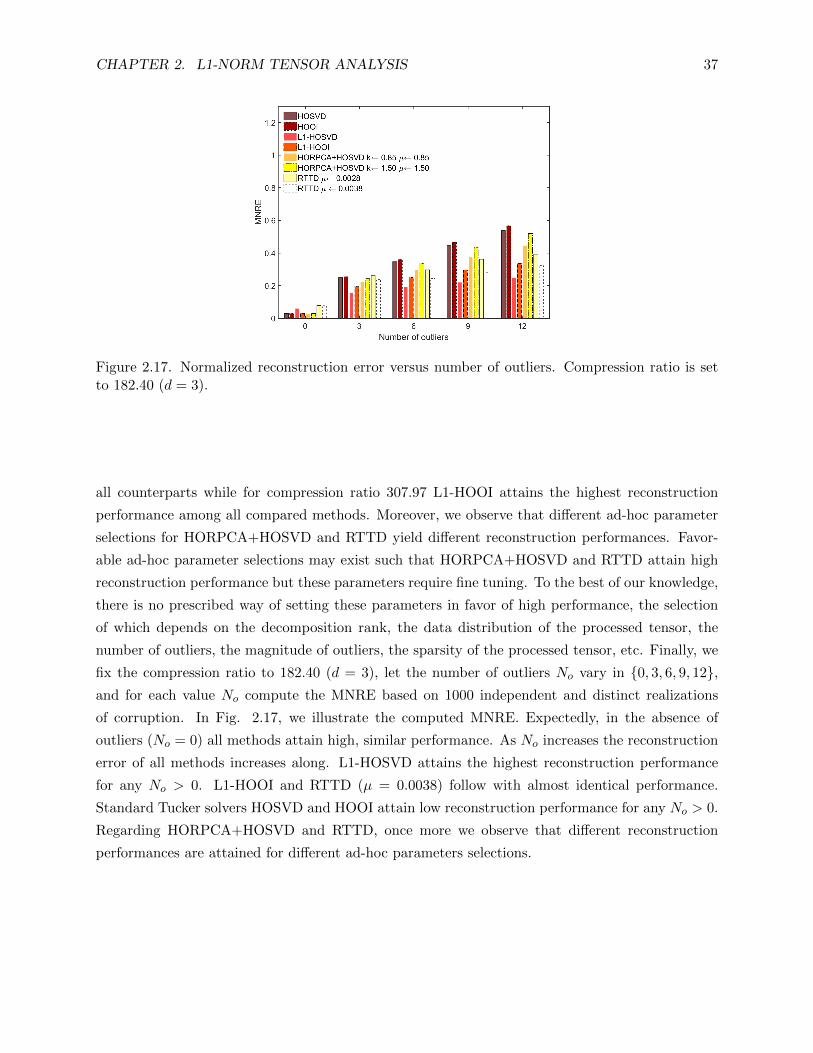
CHAPTER 2. L1-NORM TENSOR ANALYSIS 37
Figure 2.17. Normalized reconstruction error versus number of outliers. Compression ratio is setto 182.40 (d = 3).
all counterparts while for compression ratio 307.97 L1-HOOI attains the highest reconstruction
performance among all compared methods. Moreover, we observe that different ad-hoc parameter
selections for HORPCA+HOSVD and RTTD yield different reconstruction performances. Favor-
able ad-hoc parameter selections may exist such that HORPCA+HOSVD and RTTD attain high
reconstruction performance but these parameters require fine tuning. To the best of our knowledge,
there is no prescribed way of setting these parameters in favor of high performance, the selection
of which depends on the decomposition rank, the data distribution of the processed tensor, the
number of outliers, the magnitude of outliers, the sparsity of the processed tensor, etc. Finally, we
fix the compression ratio to 182.40 (d = 3), let the number of outliers No vary in 0, 3, 6, 9, 12,and for each value No compute the MNRE based on 1000 independent and distinct realizations
of corruption. In Fig. 2.17, we illustrate the computed MNRE. Expectedly, in the absence of
outliers (No = 0) all methods attain high, similar performance. As No increases the reconstruction
error of all methods increases along. L1-HOSVD attains the highest reconstruction performance
for any No > 0. L1-HOOI and RTTD (µ = 0.0038) follow with almost identical performance.
Standard Tucker solvers HOSVD and HOOI attain low reconstruction performance for any No > 0.
Regarding HORPCA+HOSVD and RTTD, once more we observe that different reconstruction
performances are attained for different ad-hoc parameters selections.
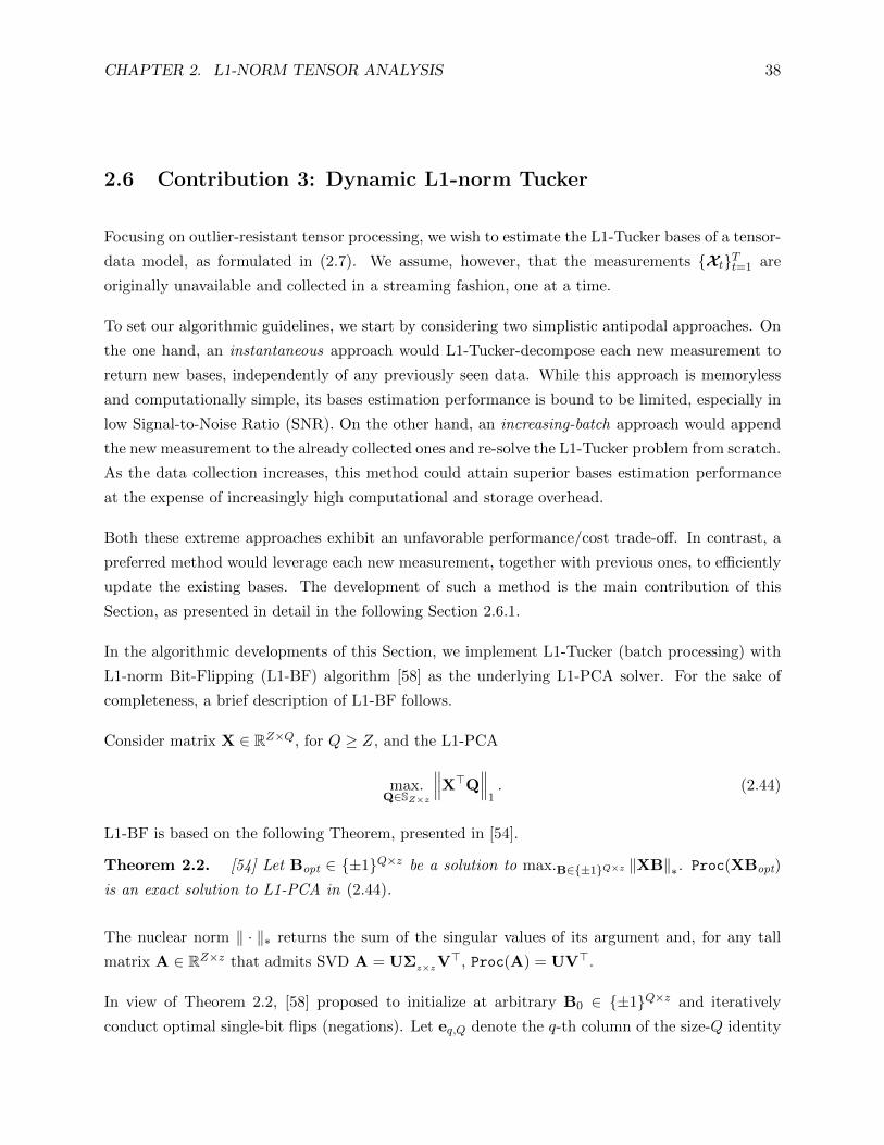
CHAPTER 2. L1-NORM TENSOR ANALYSIS 38
2.6 Contribution 3: Dynamic L1-norm Tucker
Focusing on outlier-resistant tensor processing, we wish to estimate the L1-Tucker bases of a tensor-
data model, as formulated in (2.7). We assume, however, that the measurements XtTt=1 are
originally unavailable and collected in a streaming fashion, one at a time.
To set our algorithmic guidelines, we start by considering two simplistic antipodal approaches. On
the one hand, an instantaneous approach would L1-Tucker-decompose each new measurement to
return new bases, independently of any previously seen data. While this approach is memoryless
and computationally simple, its bases estimation performance is bound to be limited, especially in
low Signal-to-Noise Ratio (SNR). On the other hand, an increasing-batch approach would append
the new measurement to the already collected ones and re-solve the L1-Tucker problem from scratch.
As the data collection increases, this method could attain superior bases estimation performance
at the expense of increasingly high computational and storage overhead.
Both these extreme approaches exhibit an unfavorable performance/cost trade-off. In contrast, a
preferred method would leverage each new measurement, together with previous ones, to efficiently
update the existing bases. The development of such a method is the main contribution of this
Section, as presented in detail in the following Section 2.6.1.
In the algorithmic developments of this Section, we implement L1-Tucker (batch processing) with
L1-norm Bit-Flipping (L1-BF) algorithm [58] as the underlying L1-PCA solver. For the sake of
completeness, a brief description of L1-BF follows.
Consider matrix X ∈ RZ×Q, for Q ≥ Z, and the L1-PCA
max.Q∈SZ×z
∥∥∥X>Q∥∥∥
1. (2.44)
L1-BF is based on the following Theorem, presented in [54].
Theorem 2.2. [54] Let Bopt ∈ ±1Q×z be a solution to max.B∈±1Q×z ‖XB‖∗. Proc(XBopt)
is an exact solution to L1-PCA in (2.44).
The nuclear norm ‖ · ‖∗ returns the sum of the singular values of its argument and, for any tall
matrix A ∈ RZ×z that admits SVD A = UΣz×zV>, Proc(A) = UV>.
In view of Theorem 2.2, [58] proposed to initialize at arbitrary B0 ∈ ±1Q×z and iteratively
conduct optimal single-bit flips (negations). Let eq,Q denote the q-th column of the size-Q identity
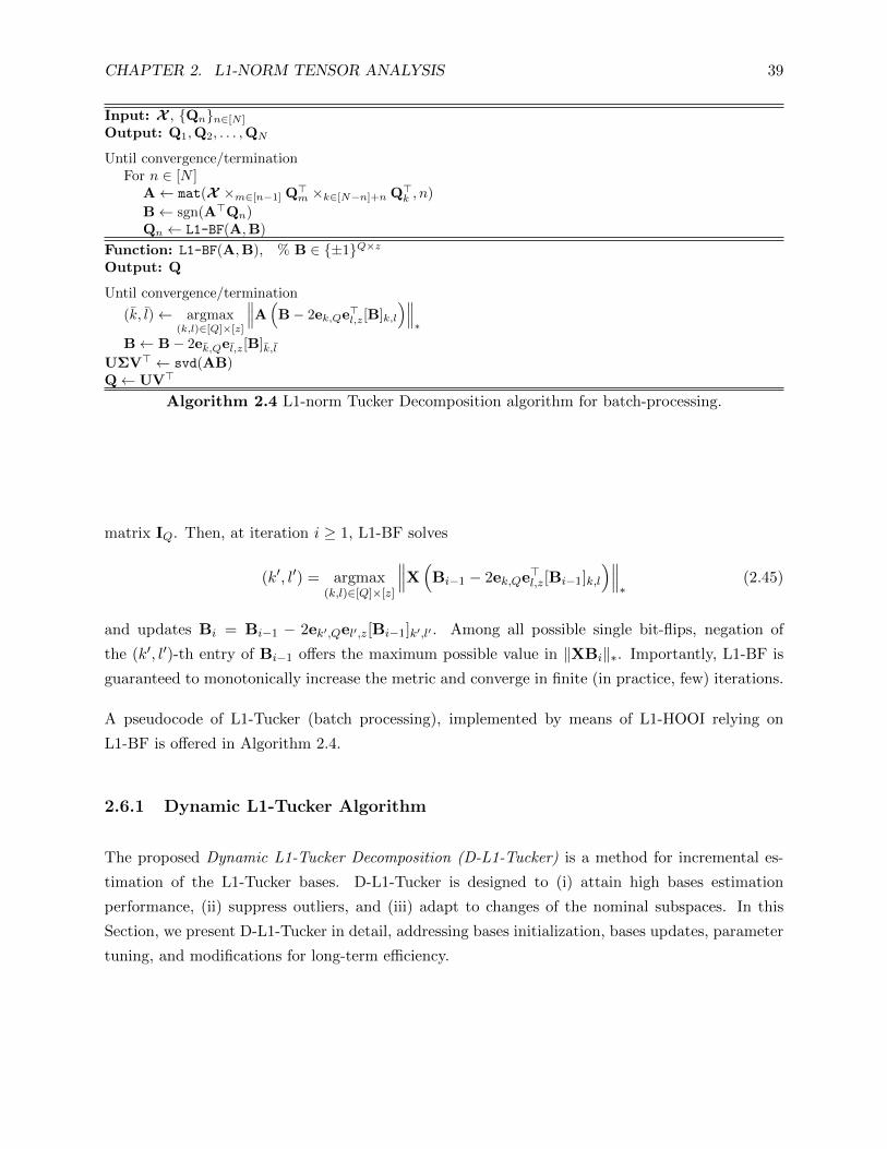
CHAPTER 2. L1-NORM TENSOR ANALYSIS 39
Input: X , Qnn∈[N ]
Output: Q1,Q2, . . . ,QN
Until convergence/terminationFor n ∈ [N ]
A← mat(X ×m∈[n−1] Q>m ×k∈[N−n]+n Q>k , n)
B← sgn(A>Qn)Qn ← L1-BF(A,B)
Function: L1-BF(A,B), % B ∈ ±1Q×zOutput: Q
Until convergence/termination
(k, l)← argmax(k,l)∈[Q]×[z]
∥∥∥A(B− 2ek,Qe>l,z[B]k,l
)∥∥∥∗
B← B− 2ek,Qel,z[B]k,lUΣV> ← svd(AB)Q← UV>
Algorithm 2.4 L1-norm Tucker Decomposition algorithm for batch-processing.
matrix IQ. Then, at iteration i ≥ 1, L1-BF solves
(k′, l′) = argmax(k,l)∈[Q]×[z]
∥∥∥X(Bi−1 − 2ek,Qe>l,z[Bi−1]k,l
)∥∥∥∗
(2.45)
and updates Bi = Bi−1 − 2ek′,Qel′,z[Bi−1]k′,l′ . Among all possible single bit-flips, negation of
the (k′, l′)-th entry of Bi−1 offers the maximum possible value in ‖XBi‖∗. Importantly, L1-BF is
guaranteed to monotonically increase the metric and converge in finite (in practice, few) iterations.
A pseudocode of L1-Tucker (batch processing), implemented by means of L1-HOOI relying on
L1-BF is offered in Algorithm 2.4.
2.6.1 Dynamic L1-Tucker Algorithm
The proposed Dynamic L1-Tucker Decomposition (D-L1-Tucker) is a method for incremental es-
timation of the L1-Tucker bases. D-L1-Tucker is designed to (i) attain high bases estimation
performance, (ii) suppress outliers, and (iii) adapt to changes of the nominal subspaces. In this
Section, we present D-L1-Tucker in detail, addressing bases initialization, bases updates, parameter
tuning, and modifications for long-term efficiency.

CHAPTER 2. L1-NORM TENSOR ANALYSIS 40
InitializationOnline update
Batch Initialization Online Updates
Ω(ℳ′ , M)
Φ(ℳt, t+1)
L1-Tucker L1-Tucker
Ω(ℬ, M)ℬ
ℳt+1
ℳ′
ℳ0
𝒬 Pass
τ
t+1
𝒬0 𝒬t
𝒬t
𝒬t+1Bases
Batch
Bases
Threshold
New data
t+1
Memory
Append
Bases
Figure 2.19. A schematic illustration of the proposed algorithm for streaming L1-norm Tuckerdecomposition.
Batch Initialization
Considering the availability of an initial batch of B T measurements, B = X1, . . . ,XB, we run
on it L1-HOSVD or L1-HOOI to obtain an initial set of L1-Tucker estimates Q0 = Q(0)1 , . . . ,Q
(0)N .
Apart from Q0, we also initialize a memory set M0 = Ω(B,M), for some maximum memory size
M ≥ 0. For any ordered set I and integer Z ≥ 0, we define
Ω(I, Z) =
I, if |I| ≤ Z,
[I]|I|−Z+1:|I|, if |I| > Z,(2.46)
where | · | denotes the cardinality (number of elements in a set) of its input argument. That is,
Ω(B,M) returns the last minM,B elements in B.
If an initialization batch B is not available, the bases in Q0 are chosen arbitrarily and the initial
memory M0 is empty. In this case, D-L1-Tucker becomes purely streaming.
Streaming Updates
When a new measurement Xt 6= 0, t ≥ 1, is collected,6 we first perform a check on it to assess its
reliability based on the most recently updated set of bases Qt−1. Motivated by [55, 77, 108, 109],
6A bar over a tensor denotes that it is streaming.

CHAPTER 2. L1-NORM TENSOR ANALYSIS 41
we define the reliability as
rt =∥∥∥Xt ×n∈[N ] Q(t−1)
n
>∥∥∥2
F
∥∥Xt
∥∥−2
F∈ [0, 1]. (2.47)
After some algebraic manipulations, (2.47) can be rewritten as
rt= cos2(φ(vec(Xt×n∈[N ]Q(t−1)n Q(t−1)
n
>), vec(Xt))), (2.48)
where φ(·, ·) returns the angle between its two vector arguments. Intuitively, rt quantifies how much
measurement Xt conforms to the multi-way subspace spanned by Q(t−1)n n∈[N ], or, the angular
proximity of vec(Xt×n∈[N ]Q(t−1)n Q
(t−1)n
>) to vec(Xt). This check of reliability/conformity inherits
its robustness from the L1-Tucker-derived bases upon which it is defined. Moreover, if an outlier
happens to pass the reliability check, L1-Tucker will try to suppress it, providing again robust
bases. By definition, the value of rt will be between 0 and 1. If rt = 1, then the bases in Qt−1
perfectly describe Xt. In contrast, if rt = 0, then the set Qt−1 does not capture any component of
Xt. Then, we introduce a user-defined parameter τ and consider that Xt is reliable for processing
if rt ≥ τ . Otherwise, Xt is considered to be an outlier and it is rejected.
If Xt passes the reliability check, we use it to update the bases and memory as follows. First, we
append the new measurement to the most recent memory set Mt−1 by computing the extended
memory M′ = Φ(Mt−1, Xt) = Mt−1 ∪ Xt. Then, we update the set of bases to Qt by running
L1-HOOI on M′, initialized to the bases in Qt−1. Finally, we update the memory by discarding
the oldest measurement, as
Mt = Ω(M′,M). (2.49)
In view of the above, the cost of the L1-HOOI algorithm remains low across updates because, at
any given instance, the extended memory M′ will comprise at most M + 1 measurements.
If Xt fails the reliability check, we discard it and update the bases and memory by settingQt = Qt−1
and Mt =Mt−1, respectively. A schematic representation of the proposed algorithm is offered in
Fig. 2.19. Here, it is worth noting that the proposed approach focuses on temporal coherence of
streaming measurements. That is, temporally sporadic points from a second nominal source of
measurements could be perceived as outliers.
CHAPTER 2. L1-NORM TENSOR ANALYSIS 42
Zero Centering
In some applications –most notable in image processing– we are interested in subspaces of zero-
centered data. To this end, we can modify the proposed algorithm so that, at every update
instance (t − 1), it computes and maintains the mean Ct−1 = (1/M)∑M
m=1[Mt−1]m. Then, when
Xt is collected, it will first be zero-centered as X ct = Xt − Ct−1. If X c
t passes the reliability check,
then it will be used to update the bases, as described above.
Adaptation to Subspace Changes
In many applications of interest, the underlying data subspaces change across time. In such cases,
an ambiguity naturally rises on whether a rejected measurement was actually an outlier or the
nominal data subspaces have changed and need to be tracked. To resolve this ambiguity and allow
D-L1-Tucker to adapt, we work as follows.
First, we make the minor assumption that outlying measurements appear sporadically. Then, we
introduce a buffer of ambiguous measurements, W, with capacity W > 0. When a streaming
measurement fails the reliability check, we insert it to W. If a measurement passes the reliability
check, then we empty W. If at any update instance |W| reaches W –i.e., W consecutive streaming
measurements were rejected as outliers– then we detect a change of the nominal subspaces.
In order to adapt to these changes, we empty the memory, set B =W, and re-initialize (reset) the
bases and memory, as described in Section 2.6.1. Next, the updates proceed as described in Section
2.6.1. A pseudocode of the proposed D-L1-Tucker algorithm is presented in Algorithm 2.5.
Long-Run Efficiency
As measurements are streaming, D-L1-Tucker keeps refining the bases estimates. Naturally, after a
sufficiently large number of measurements have been processed, the enhancement rate of the bases
estimates can be so low that does not justify the computational effort expended for the update.
In view of this observation, we can enhance the long-run efficiency of D-L1-Tucker by introducing
an exponentially decreasing probability ρt to determine whether or not the t-th measurement will
be processed. Intuitively, when a large number of reliable measurements have been processed, ρt
should be low enough to limit the number of updates performed. For example, let us denote by αt−1
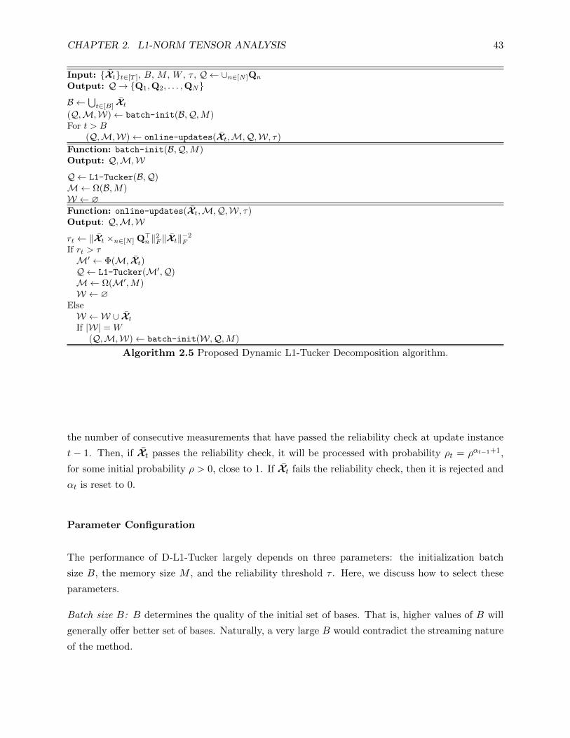
CHAPTER 2. L1-NORM TENSOR ANALYSIS 43
Input: Xtt∈[T ], B, M , W , τ , Q ← ∪n∈[N ]Qn
Output: Q → Q1,Q2, . . . ,QN
B ←⋃
t∈[B] Xt
(Q,M,W)← batch-init(B,Q,M)For t > B
(Q,M,W)← online-updates(Xt,M,Q,W, τ)
Function: batch-init(B,Q,M)Output: Q,M,W
Q← L1-Tucker(B,Q)M← Ω(B,M)W ← ∅Function: online-updates(Xt,M,Q,W, τ)Output: Q,M,W
rt ← ‖Xt ×n∈[N ] Q>n ‖2F ‖Xt‖−2F
If rt > τM′ ← Φ(M, Xt)Q ← L1-Tucker(M′,Q)M← Ω(M′,M)W ← ∅
ElseW ←W ∪ Xt
If |W| = W(Q,M,W)← batch-init(W,Q,M)
Algorithm 2.5 Proposed Dynamic L1-Tucker Decomposition algorithm.
the number of consecutive measurements that have passed the reliability check at update instance
t − 1. Then, if Xt passes the reliability check, it will be processed with probability ρt = ραt−1+1,
for some initial probability ρ > 0, close to 1. If Xt fails the reliability check, then it is rejected and
αt is reset to 0.
Parameter Configuration
The performance of D-L1-Tucker largely depends on three parameters: the initialization batch
size B, the memory size M , and the reliability threshold τ . Here, we discuss how to select these
parameters.
Batch size B: B determines the quality of the initial set of bases. That is, higher values of B will
generally offer better set of bases. Naturally, a very large B would contradict the streaming nature
of the method.
CHAPTER 2. L1-NORM TENSOR ANALYSIS 44
Memory size M : M determines how many measurements L1-Tucker will process at each time
instance. Similar to B, higher values of M can enable superior estimation performance. At the
same time, high values of M increase the overhead of storage and computation (cost of L1-Tucker
updates). Thus, a rule of thumb is to set M as high as the storage/computation limitations of the
application permit.
Reliability threshold τ : For τ = 0, all measurements will be processed (including outliers); for τ = 1,
all measurements will fail the reliability check and no bases updates will take place. Appropriate
tuning of τ between 0 and 1 may ask for some prior knowledge on the SNR quality of the nominal
data. Alternatively, in the sequel we present a data-driven method for setting τ .
We start with the reasonable assumption that the initialization batch B is outlier-free. Then, we
conduct on B a leave-one-out cross-validation to tune τ . For every i ∈ [B], we first form Bi = B\Xi.
Then, we obtain the set of basesQi by running L1-HOOI on Bi. Next, we capture in ri the reliability
of Xi evaluated on Qi (notice that Xi did not participate in the computation of Qi). Finally, we
set τ to the minimum, median, or maximum value of the cross-validated reliabilities r1, . . . , rB,depending on the noise-tolerance/outlier-robustness level that we want to enforce.
2.6.2 Experimental Studies
Testing Parameter Configurations
We first study the performance of the proposed D-L1-Tucker algorithm across varying parameter
configurations. We consider T N -way measurements X1, . . . , XT , where
Xt = Gt ×n∈[N ] Qnomn + Nt + Ot ∈ RD×D×...×D, (2.50)
for a nominal set of bases Qnom = Qnomn ∈ SD×dn∈[N ]. The core tensor Gt ∈ Rd×d×...×d draws
entries independently from N (0, σ2s). Nt models Additive White Gaussian Noise (AWGN) and
draws entries from N (0, σ2n). Ot models sporadic heavy outlier corruption and is non-zero with
probability po. When non-zero, Ot draws entries from N (0, σ2o). In order to measure data quality,
we define the SNR as
SNR =E‖Xt‖2F E‖Nt‖2F
=σ2s
σ2n
(d
D
)N(2.51)

CHAPTER 2. L1-NORM TENSOR ANALYSIS 45
5 10 15 20M
0
0.005
0.01
0.015
0.02
0.025
MA
NS
SE
po=0.1, =0
po=0.06, =0.4
po=0.1, =0.6
po=0.06, =0.7
Figure 2.21. MANSSE vs memory size. N = 3, D = 10, d = 5, B = 5, T = 30, SNR = 0dB, ONR= 14dB, 3000 realizations.
0 0.1 0.2 0.3 0.4 0.5 0.6 0.72
4
6
8
10
12
14
16
MA
NS
SE
10-3
po=0
po=0.02
po=0.04
po=0.05
po=0.06
po=0.08
po=0.1
Figure 2.22. MANSSE vs reliability threshold. N = 3, D = 10, d = 5, B = 5, M = 10, T = 30,SNR = 0dB, ONR = 14dB, 3000 realizations.
and the Outlier-to-Noise Ratio (ONR)
ONR =E‖Ot‖2F E‖Nt‖2F
=σ2o
σ2n
. (2.52)
Our objective is to recover Qnom by processing the measurements Xtt∈[T ] in a streaming way.
Denoting by Qn the estimate of Qnomn , we quantify performance by means of the Mean Aggregate
Normalized Subspace Squared Error (MANSSE)
MANSSE =1
2Nd
∑n∈[N ]
∥∥∥Qnomn Qnom
n> − QnQ
>n
∥∥∥2
F. (2.53)
First, we set N = 3, D = 10, d = 5, B = 5, and T = 30. Moreover, we set σ2s , σ
2n, and σ2
o such
that SNR = 0dB and ONR = 14dB. In Fig. 2.21, we plot the MANSSE metric versus varying
M ∈ 5, 10, 15, 20 and fixed (p0, τ) ∈ (0.1, 0), (0.06, 0.4), (0.1, 0.6), (0.06, 0.7). We observe that
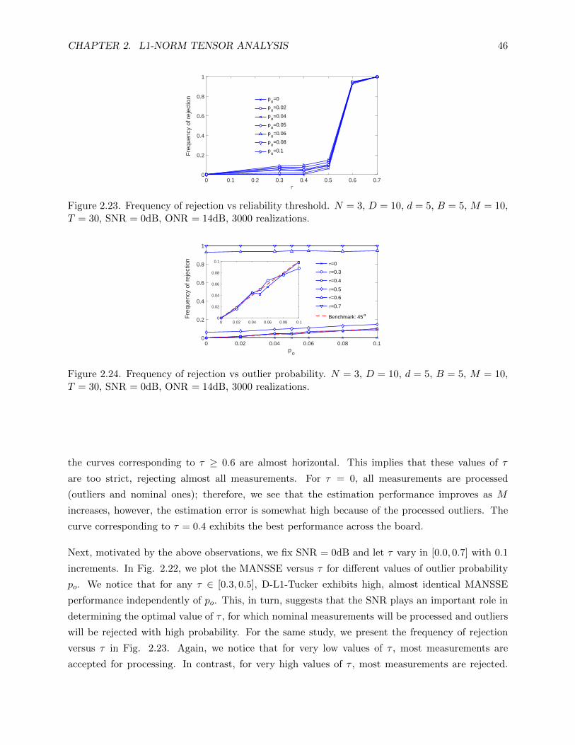
CHAPTER 2. L1-NORM TENSOR ANALYSIS 46
0 0.1 0.2 0.3 0.4 0.5 0.6 0.70
0.2
0.4
0.6
0.8
1
Fre
quen
cy o
f rej
ectio
n po=0
po=0.02
po=0.04
po=0.05
po=0.06
po=0.08
po=0.1
Figure 2.23. Frequency of rejection vs reliability threshold. N = 3, D = 10, d = 5, B = 5, M = 10,T = 30, SNR = 0dB, ONR = 14dB, 3000 realizations.
0 0.02 0.04 0.06 0.08 0.1po
0
0.2
0.4
0.6
0.8
1
Fre
quen
cy o
f rej
ectio
n
=0
=0.3
=0.4
=0.5
=0.6
=0.7
Benchmark: 45o
0 0.02 0.04 0.06 0.08 0.10
0.02
0.04
0.06
0.08
0.1
Figure 2.24. Frequency of rejection vs outlier probability. N = 3, D = 10, d = 5, B = 5, M = 10,T = 30, SNR = 0dB, ONR = 14dB, 3000 realizations.
the curves corresponding to τ ≥ 0.6 are almost horizontal. This implies that these values of τ
are too strict, rejecting almost all measurements. For τ = 0, all measurements are processed
(outliers and nominal ones); therefore, we see that the estimation performance improves as M
increases, however, the estimation error is somewhat high because of the processed outliers. The
curve corresponding to τ = 0.4 exhibits the best performance across the board.
Next, motivated by the above observations, we fix SNR = 0dB and let τ vary in [0.0, 0.7] with 0.1
increments. In Fig. 2.22, we plot the MANSSE versus τ for different values of outlier probability
po. We notice that for any τ ∈ [0.3, 0.5], D-L1-Tucker exhibits high, almost identical MANSSE
performance independently of po. This, in turn, suggests that the SNR plays an important role in
determining the optimal value of τ , for which nominal measurements will be processed and outliers
will be rejected with high probability. For the same study, we present the frequency of rejection
versus τ in Fig. 2.23. Again, we notice that for very low values of τ , most measurements are
accepted for processing. In contrast, for very high values of τ , most measurements are rejected.
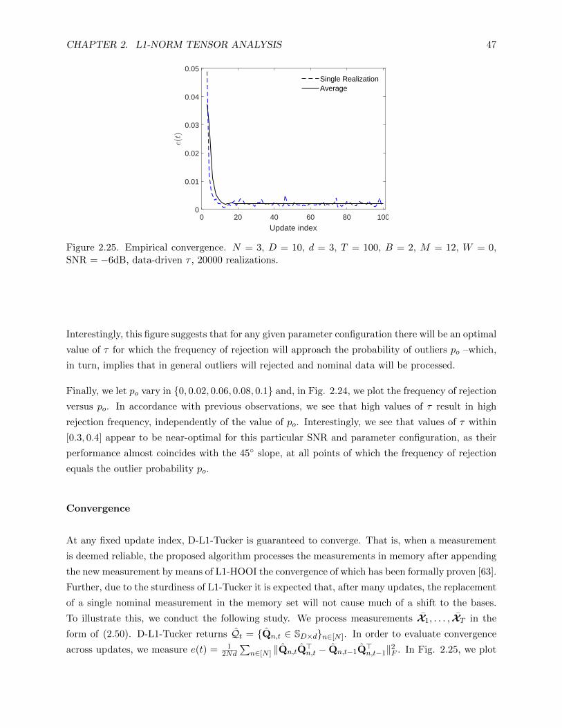
CHAPTER 2. L1-NORM TENSOR ANALYSIS 47
0 20 40 60 80 100
Update index
0
0.01
0.02
0.03
0.04
0.05Single RealizationAverage
Figure 2.25. Empirical convergence. N = 3, D = 10, d = 3, T = 100, B = 2, M = 12, W = 0,SNR = −6dB, data-driven τ , 20000 realizations.
Interestingly, this figure suggests that for any given parameter configuration there will be an optimal
value of τ for which the frequency of rejection will approach the probability of outliers po –which,
in turn, implies that in general outliers will rejected and nominal data will be processed.
Finally, we let po vary in 0, 0.02, 0.06, 0.08, 0.1 and, in Fig. 2.24, we plot the frequency of rejection
versus po. In accordance with previous observations, we see that high values of τ result in high
rejection frequency, independently of the value of po. Interestingly, we see that values of τ within
[0.3, 0.4] appear to be near-optimal for this particular SNR and parameter configuration, as their
performance almost coincides with the 45 slope, at all points of which the frequency of rejection
equals the outlier probability po.
Convergence
At any fixed update index, D-L1-Tucker is guaranteed to converge. That is, when a measurement
is deemed reliable, the proposed algorithm processes the measurements in memory after appending
the new measurement by means of L1-HOOI the convergence of which has been formally proven [63].
Further, due to the sturdiness of L1-Tucker it is expected that, after many updates, the replacement
of a single nominal measurement in the memory set will not cause much of a shift to the bases.
To illustrate this, we conduct the following study. We process measurements X1, . . . , XT in the
form of (2.50). D-L1-Tucker returns Qt = Qn,t ∈ SD×dn∈[N ]. In order to evaluate convergence
across updates, we measure e(t) = 12Nd
∑n∈[N ] ‖Qn,tQ
>n,t − Qn,t−1Q
>n,t−1‖2F . In Fig. 2.25, we plot

CHAPTER 2. L1-NORM TENSOR ANALYSIS 48
0 20 40 60 80 100
Update index
0
0.2
0.4
0.6
0.8
1
MA
NS
SE
D-L1-TUCKER (proposed)DTA ( =0.2)DTA ( =0.8)LRUT (k=D-d-2)HOSVD (inst.)OUTLIERSUBSPACE CHANGE
Figure 2.26. MANSSE vs update index. N = 3, D = 10, d = 3, T1 = 70, T2 = 30, B = 2, M = 12,W = 4, SNR = −6dB, ONR = 18dB, data-driven τ , 20000 realizations.
e(t) versus update index t for a single realization of measurements. Moreover, we plot e(t) when it
is sample-average computed over 20000 statistically independent realizations of measurements. As
expected, we see that after enough measurements have been processed, e(t) remains low and very
close to the average expected performance. We conclude that, upon nominal operation and large
enough M , bases changes will be minuscule in the long run. This will be even more emphatic for
high SNR. Finally, the long-run efficiency feature of D-L1-Tucker, introduced in Section 2.6.1, can
also enforce convergence/termination.
Dynamic Subspace Adaptation
We consider a total of T = T1 + T2 streaming measurements, in the form of (2.50). The first
T1 measurements are generated by nominal bases Qnom,1. For t > T1 and on, the measure-
ments are generated by bases Qnom,2. The angular proximity of Qnom,1n to Qnom,2
n , defined as
1 − ‖Qnom,1n Qnom,1
n> − Qnom,2
n Qnom,2n
>‖2F (2d)−1, is set between 30% and 40% for every n ∈ [N ].
Moreover, we consider that the outlier is only active at instance t = to = 45. We set N = 3,
D = 10, d = 3, T1 = 70, and T2 = 30. The SNR and ONR are set to −6dB and 18dB, respectively.
We process all measurements by the proposed D-L1-Tucker algorithm for B = 2, M = 12, W = 4,
and data-driven τ (median of cross-validated batch reliabilities). We also process the streaming
measurements with DTA (λ = 0.2, 0.8), LRUT (additional core dimensions k = D − d − 2), and
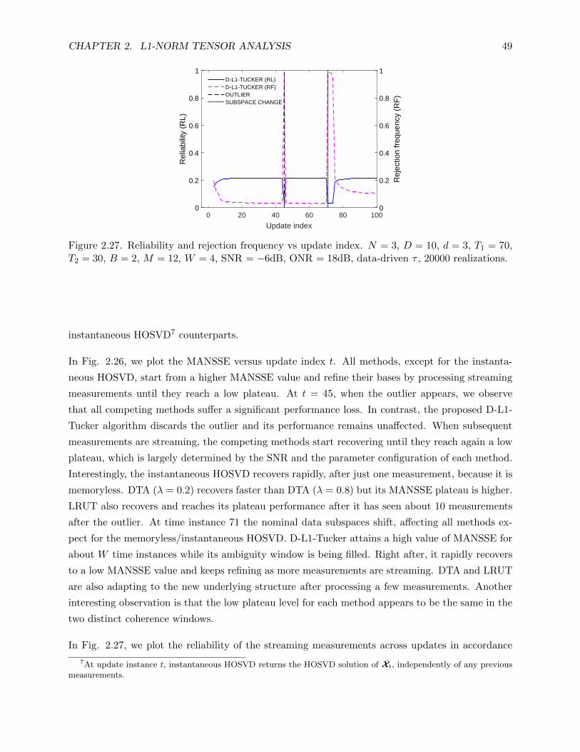
CHAPTER 2. L1-NORM TENSOR ANALYSIS 49
0 20 40 60 80 100
Update index
0
0.2
0.4
0.6
0.8
1
Rel
iabi
lity
(RL)
0
0.2
0.4
0.6
0.8
1
Rej
ectio
n fr
eque
ncy
(RF
)
D-L1-TUCKER (RL)D-L1-TUCKER (RF)OUTLIERSUBSPACE CHANGE
Figure 2.27. Reliability and rejection frequency vs update index. N = 3, D = 10, d = 3, T1 = 70,T2 = 30, B = 2, M = 12, W = 4, SNR = −6dB, ONR = 18dB, data-driven τ , 20000 realizations.
instantaneous HOSVD7 counterparts.
In Fig. 2.26, we plot the MANSSE versus update index t. All methods, except for the instanta-
neous HOSVD, start from a higher MANSSE value and refine their bases by processing streaming
measurements until they reach a low plateau. At t = 45, when the outlier appears, we observe
that all competing methods suffer a significant performance loss. In contrast, the proposed D-L1-
Tucker algorithm discards the outlier and its performance remains unaffected. When subsequent
measurements are streaming, the competing methods start recovering until they reach again a low
plateau, which is largely determined by the SNR and the parameter configuration of each method.
Interestingly, the instantaneous HOSVD recovers rapidly, after just one measurement, because it is
memoryless. DTA (λ = 0.2) recovers faster than DTA (λ = 0.8) but its MANSSE plateau is higher.
LRUT also recovers and reaches its plateau performance after it has seen about 10 measurements
after the outlier. At time instance 71 the nominal data subspaces shift, affecting all methods ex-
pect for the memoryless/instantaneous HOSVD. D-L1-Tucker attains a high value of MANSSE for
about W time instances while its ambiguity window is being filled. Right after, it rapidly recovers
to a low MANSSE value and keeps refining as more measurements are streaming. DTA and LRUT
are also adapting to the new underlying structure after processing a few measurements. Another
interesting observation is that the low plateau level for each method appears to be the same in the
two distinct coherence windows.
In Fig. 2.27, we plot the reliability of the streaming measurements across updates in accordance
7At update instance t, instantaneous HOSVD returns the HOSVD solution of Xt, independently of any previousmeasurements.

CHAPTER 2. L1-NORM TENSOR ANALYSIS 50
0 20 40 60 80 100
Update index
0
0.01
0.02
0.03
0.04
0.05
0.06
0.07
0.08
Tim
e (s
ec.)
D-L1-TUCKER (proposed)DTA ( =0.2)DTA ( =0.8)LRUT (k=D-d-2)HOSVD (inst.)OUTLIERSUBSPACE CHANGE
Figure 2.28. Time (sec.) vs update index. N = 3, D = 10, d = 3, T1 = 70, T2 = 30, B = 2,M = 12, W = 4, SNR = −6dB, ONR = 18dB, data-driven τ , 20000 realizations.
0 20 40 60 80 100 120 140 160
Update index
0
0.2
0.4
0.6
0.8
1
MA
NS
SE
D-L1-TUCKER (proposed)D-TUCKERDTA ( =0.2)DTA ( =0.8)LRUT (k=D-d-2)HOSVD (inst.)SUBSPACE CHANGE
Figure 2.29. MANSSE vs update index. N = 3, D = 10, d = 3, T1 = 75, T2 = 85, B = 2, M = 12,W = 4, SNR = −6dB, ONR = 18dB, data-driven τ , 20000 realizations.
with (2.47). At the same figure, we illustrate the frequency of rejection; that is, the frequency
by which measurements fail the reliability check. We notice that the outlier at t = 45 and the
W measurements following the change of subspaces are rejected with probability close to 1. In
addition, we observe the instantaneous reliability drop when the outlier appears and when nominal
subspaces change. For this value of SNR = −6dB, the reliability level for nominal measurements
is about 0.2 and our data-driven τ is accordingly low.
We conclude this study by comparing the run time of each method across updates. In Fig. 2.28,

CHAPTER 2. L1-NORM TENSOR ANALYSIS 51
0 50 100 150
Update index
0
0.2
0.4
0.6
0.8
1
Rel
iabi
lity
(RL)
0
0.2
0.4
0.6
0.8
1
Rej
ectio
n fr
eque
ncy
(RF
)
D-L1-TUCKER (RL)D-L1-TUCKER (RF)D-TUCKER (RL)D-TUCKER (RF)SUBSPACE CHANGE
Figure 2.30. Reliability and rejection frequency vs update index. N = 3, D = 10, d = 3, T1 = 75,T2 = 85, B = 2, M = 12, W = 4, SNR = −6dB, ONR = 18dB, data-driven τ , 20000 realizations.
we plot the instantaneous run times. We observe that the instantaneous HOSVD and DTA exhibit
constant run time across updates independently of outliers or changes of subspaces. D-L1-Tucker
also exhibits about constant runtime after its memory has been filled. Moreover, we notice an
instantaneous drop in the runtime at index t = 45 which is because D-L1-Tucker discarded the
outlier and did not process it. In contrast, when the outlier appears and when the subspaces
change, LRUT attains an increase in runtime, as it tries to adapt.
Next, we repeat the above study. This time, instead of having a fixed outlier at an index, every
measurement with index t > B is outlier corrupted with probability po = 0.1. Moreover, T1 = 75
and T2 = 85. This time, we include a curve which corresponds to a method we label D-Tucker.
D-Tucker is identical to D-L1-Tucker with the exception that standard Tucker by means of HOOI
is employed instead of L1-Tucker.
In Fig. 2.29, we plot the MANSSE versus update index. We observe that the estimation perfor-
mance of the DTA curves degrades due to the outliers until a plateau is reached. Their estimation
error increases at the subspaces change index and returns to its plateau performance after a few
measurements. Expectedly, the instantaneous HOSVD appears to exhibit constant performance for
any index t > B. A similar observation is made for the LRUT curve with the exception of update
indices 75 to 80 where it adjusts to the new underlying data structure. D-Tucker starts from a low
MANSSE value and improves for a while, however, its performance slowly drops as measurements
are streaming. This is because outliers are passing the reliability check of the L2-norm derived
bases which, in turn, affects the performance of the memory batch processing. In contrast, we see
that D-L1-Tucker keeps improving its performance up to update index 75 where the underlying

CHAPTER 2. L1-NORM TENSOR ANALYSIS 52
(a) (b) (c) (d)
(e) (f) (g) (h)
(i) (j) (k) (l)
(m) (n) (o) (p)
(q)
Figure 2.31. Dynamic video foreground/background separation experiment. (a) Original 75-thframe (scene 1). Background extracted by (b) Adaptive Mean (λ = 0.95), (c) DTA (λ = 0.95), (d)DTA (λ = 0.7), (e) LRUT, (f) OSTD, (g) HOOI (increasing memory), (h) L1-HOOI (increasingmemory), and (i) D-L1-TUCKER (proposed). Foreground extracted by (j) Adaptive Mean (λ =0.95), (k) DTA (λ = 0.95), (l) DTA (λ = 0.7), (m) LRUT, (n) OSTD, (o) HOOI (increasingmemory), (p) L1-HOOI (increasing memory), and (q) D-L1-TUCKER (proposed).
data structure changes. Then, after the ambiguity batch windows of D-Tucker and D-L1-Tucker
are filled, they both reset based on the measurements in their window –each measurement of which

CHAPTER 2. L1-NORM TENSOR ANALYSIS 53
(a) (b) (c) (d)
(e) (f) (g) (h)
(i) (j) (k) (l)
(m) (n) (o) (p)
(q)
Figure 2.32. Dynamic video foreground/background separation experiment. (a) Original 150-thframe (scene 2). Background extracted by (b) Adaptive Mean (λ = 0.95), (c) DTA (λ = 0.95), (d)DTA (λ = 0.7), (e) LRUT, (f) OSTD, (g) HOOI (increasing memory), (h) L1-HOOI (increasingmemory), and (i) D-L1-TUCKER (proposed). Foreground extracted by (j) Adaptive Mean (λ =0.95), (k) DTA (λ = 0.95), (l) DTA (λ = 0.7), (m) LRUT, (n) OSTD, (o) HOOI (increasingmemory), (p) L1-HOOI (increasing memory), and (q) D-L1-TUCKER (proposed).
is outlier corrupted with probability po. Due to its inherent L1-norm robustness, D-L1-Tucker is
able to recover and learn the underlying data structure of the new coherence window. In contrast,
CHAPTER 2. L1-NORM TENSOR ANALYSIS 54
we see that D-Tucker fails to recover due to the outlying measurements in its ambiguity window.
In Fig. 2.30, we illustrate the reliability values and rejection frequencies as they were computed by
the proposed D-L1-Tucker and its counterpart D-Tucker. We observe that during the first coherence
window (t ≤ T1), both methods exhibit almost identical reliabilities and rejection frequencies.
However, in view of Fig. 2.29, we infer that D-L1-Tucker is more successful at rejecting outliers
compared to D-Tucker. A few measurements after the change of subspaces at index t = 75, we
see that D-L1-Tucker converges to reliability and rejection frequency values similar to those of the
first coherence window which implies that it has adapted nicely to the new coherence window.
On the other hand, the reliability and rejection frequency values to which D-Tucker converges in
the second coherence window, both diverge from their corresponding values in the first coherence
window which, in turn, implies that D-Tucker was not able to adapt well. This is also depicted
in Fig. 2.29 where we see that in the second coherence window D-Tucker converged to a high
MANSSE value.
Dynamic Video Foreground/Background Separation
Foreground-background separation is a common task in video processing applications, including
moving object tracking, security surveillance, and traffic monitoring. The omnipresent background
in a static camera scene determines a nominal subspace, while any foreground movement –e.g.,
by vehicles or people– represent intermittent outliers. In this experiment, we use D-L1-Tucker to
estimate the background and foreground of incoming video frames and compare its performance
with that of state-of-the-art alternatives.
For this experiment, we use videos from the CAVIAR database [110]. Specifically, we use two
videos, each containing 100 frames of size (D1 = 173)× (D2 = 231) and capturing a different scene.
Each video is viewed as collection of frames –i.e., 2-way tensor measurements. We collate the two
videos, one behind the other to form the data stream X ∈ RD1×D2×(T=200). Below, we denote by
Xt the t-th frontal slab of X (i.e., the t-th video frame).
We apply the proposed algorithm on X by setting dn = d = 3 ∀n ∈ [2], B = 5, M = 10,
W = 20, and τ by the proposed batch reliability cross-validation. For every t ∈ [T − B] + B, we
obtain bases Q(t)1 and Q
(t)2 and the mean frame Ct. Accordingly, we estimate the background as
XBGt = Q
(t)1 Q
(t)2
> (Xt − Ct
)Q
(t)2 Q
(t)2
>+ Ct and the foreground as XFG
t = Xt −XBGt .

CHAPTER 2. L1-NORM TENSOR ANALYSIS 55
We compare the performance of the proposed algorithm with that of DTA, LRUT, OSTD,8 HOOI
(increasing batch), and L1-HOOI (increasing batch). For the last two benchmark approaches, at
any frame index t, we run HOOI/L1-HOOI on the entire batch Xjj∈[t], starting from arbitrary
initialization. We notice that DTA is capable of tracking scene changes using a forgetting factor λ.
Since the background estimation involves mean subtraction, for a fair comparison with the proposed
method, we enable mean tracking for DTA by computing CDTAt = λCDTA
t−1 +(1−λ)Xt, for CDTA1 = X1.
For all other methods, we compute the mean incrementally at any t as Ct =((t− 1)Ct−1 + Xt
)/t.
For DTA, we use two values of forgetting factor, λ = 0.95, 0.7 and for LRUT we set the number of
additional core dimensions to kn = Dn − d− 3 ∀n ∈ [2].
In Fig. 2.31 and Fig. 2.32, we present the backgrounds and foregrounds obtained by the proposed
method and existing counterparts at the 75-th frame (scene 1) and the 150-th frame (scene 2),
respectively. We observe from Fig. 2.31 that HOOI (increasing batch), LRUT, and OSTD perform
similarly leaving a trail of a ghostly appearance behind the person in their respective foreground
frames. We notice that OSTD and L1-HOOI (increasing batch) perform better with a smoother
trail behind the person in their foreground frames. DTA with λ = 0.7 captures the person in
its background, leading to an undesirably smudged foreground estimate. DTA with λ = 0.95
demonstrates a cleaner foreground estimate, similar to that of the adaptive mean (background
estimated by the same adaptive mean that we use for DTA), however their backgrounds contain
a ghostly appearance of the person. The proposed method extracts a cleaner background and
foreground owing to its outlier rejection capability.
In Fig. 2.32, we demonstrate the performance after the scene changes at t = 100 by presenting the
estimated backgrounds and foregrounds at frame index t = 150. We observe that HOOI, L1-HOOI,
OSTD, and LRUT perform poorly because they are not designed to track changes in the scene.
DTA with λ = 0.95 demonstrates better performance compared to that of λ = 0.75 at frame 75,
however, at frame 150, we observe that DTA with λ = 0.9 captures some of the background from
scene 1, while DTA with λ = 0.7 obtains a clean background and hence a smooth foreground,
wherein the person appears slightly blurry. The proposed method is capable of tracking scene
changes and we observe that it obtains a good estimate of the background and a clear foreground.
To quantify the background/foreground estimation performance, we compute, for every frame, the
Peak Signal-to-Noise Ratio (PSNR) defined as PSNR = 10log10
(2552
MSE
), where MSE is the mean
squared error of the estimated background and the ground truth (clean) background. In Fig. 2.33,
we plot the PSNR versus frame index and observe that all methods begin with high PSNR and, as
8OSTD –i.e., Online Stochastic Tensor Decomposition– was specifically designed for background/foreground sep-aration in multispectral video sequences [91].

CHAPTER 2. L1-NORM TENSOR ANALYSIS 56
50 100 150 200
Frame Index
-10
0
10
20
30
40
50
PS
NR
(dB
)
DTA ( = 0.95)DTA ( = 0.7)LRUTOSTDHOOIL1-HOOIADAPTIVE MEAN( = 0.95)D-L1-TUCKER (proposed)RETROACTIVE COMPUTATION (proposed)SCENE CHANGE
Figure 2.33. Dynamic video foreground/background separation experiment. PSNR (dB) versusframe index.
0 10 20 30 40 50 60 70 80
Measurement Index
0.5
0.6
0.7
0.8
0.9
1
Ave
rage
Cla
ssifi
catio
n A
ccur
acy
D-L1-TUCKER (proposed) + OSVMDTA ( =0.33) + OSVMOSTD + OSVMOSVM
Noisy data
Clean data
Figure 2.34. Online tensor compression and classification experiment. Average classification accu-racy versus update index.
they process frames with foreground movement, the PSNR drops. We observe that the PSNR of the
proposed method is the highest after approximately frame 25. When the scene changes, the PSNR
of all methods drops instantaneously. The PSNR values of HOOI, L1-HOOI, LRUT, and OSTD
increase at a low rate as they process frames from the new scene. Adaptive mean and DTA with
λ = 0.95 demonstrate better performance with faster PSNR increase. DTA with λ = 0.5 adapts
to the new scene very quickly, but it is affected by foreground movement (depicted by oscillations
in its PSNR values). The proposed method adapts to the new scene after it processes W = 20
CHAPTER 2. L1-NORM TENSOR ANALYSIS 57
measurements and attains the highest PSNR values across all frame indices thereafter. Certainly,
after adaptation, the proposed method is straightforwardly capable of accurately extracting the
background and foreground of all ambiguous frames inW in a retroactive fashion, as shown in Fig.
2.33.
Online Tucker and Classification
In this experiment, we perform joint Tucker feature extraction and online classification. We use
the Extended Yale Face Database B [99], consisting of face images of many individuals, captured at
varying illumination. For this experiment, we use the face images of subject 02 and subject 23 to
perform binary classification. Each class has 64 images in total, out of which, at every realization,
we choose 45 for training and the remaining 19 for testing. The size of each image is originally
192 × 168 and we down-sample it to 96 × 84. Therefore, at every realization, we have a tensor
with training data X ∈ R96×84×90 containing 90 measurements in total (45 from each class) and a
tensor with testing data Y ∈ R96×84×38 containing 38 measurements in total (19 from each class).
At every realization, we arbitrarily shuffle the training data and follow a parallel online feature
extraction and classification approach as follows.
At update index t, we process the t-th training sample in X , Xt, and update Q(t)1 and Q
(t)2 using
the proposed method (B = 5, M = 10, d1 = 15, d2 = 6, and cross-validated τ). Next, we use
the updated bases to compress all previously seen training data Xii∈[t] as Zi = Q(t)1
>XiQ
(t)2 .
We vectorize the compressed training measurements and give them as input to the Online Support
Vector Machine (OSVM) classifier of [111].9 We test the performance of the classifier on testing
data, compressed using the same bases, and record the classification accuracy for every update
index t. We repeat the experiment 300 times and plot the average classification accuracy versus
update index in Fig. 2.34. Along with the proposed algorithm, we also plot the performance of
the plain OSVM classifier, i.e., OSVM classifier run on vectorized (uncompressed) data, DTA with
λ = 0.33, and OSTD. In Fig. 2.34, we observe that all compared methods attain almost identical
performance. The classification accuracy starts low and as the update index increases it tends to
1.
Next, we repeat the experiment with the same setting, by corrupting each training measurement
outside the initial memory batch B with noise from N (2, 5), cropping pixel intensities outside
[0, 255]. We compute the average classification accuracy over 300 realizations and plot it versus
9Matlab code available at https://www.cpdiehl.org/code.html.

CHAPTER 2. L1-NORM TENSOR ANALYSIS 58
(a) (b) (c) (d)
(e) (f) (g) (h)
(i)
Figure 2.35. Frame instances per scene for the three videos. Video 1: (a) scene 1, (b) scene 2, and(c) noisy frame. Video 2: (d) scene 1, (e) scene 2, and (f) noisy frame. Video 3: (g) scene 1, (h)scene 2, and (i) noisy frame. Probability of noise corruption per pixel is 10% for all noisy frames.
update index in Fig. 2.34. In this case, we notice that plain OSVM is significantly affected by the
noise. DTA, OSTD, and D-L1-Tucker demonstrate resistance to noise corruption, especially for
earlier update indices.
Online Video Scene Change Detection
In this experiment, we demonstrate the efficacy of the proposed method in online video scene change
detection. We operate on Red-Green-Blue (RGB) videos from the benchmark video scene change
detection dataset in [112]. Specifically, we operate on three video frame-sequences from the dataset.
Video 1 (twoPositionPTZCam) captures a street with a single scene change. Video 2 (badminton)
captures badminton players in action with camera jittering. Video 3 (zoomInzoomOut) captures
the backyard of a house with a single scene change. Each video can be seen as a collection of 3-way
tensors Xt ∈ RD1×D2×D3 which are the video frames streaming across time t = 1, 2, . . .. Videos 1,
2, and 3 are cropped to consist of T = 202, 220, and 172 frames, respectively, and each frame is
of size 85× 143× 3, 94× 144× 3, and 60× 80× 3, respectively. For videos 1 and 3, scene change

CHAPTER 2. L1-NORM TENSOR ANALYSIS 59
0 0.5 1Corruption probability (%)
95
96
97
98
99
100
Ave
rage
acc
urac
y (%
)
0 1 2Corruption probability (%)
94
95
96
97
98
99
100
Ave
rage
acc
urac
y (%
)
0 1 2Corruption probability (%)
95
96
97
98
99
100
Ave
rage
acc
urac
y (%
)
SSCD HOOI+SSCD DTA (λ=0.2)+SSCD L1-HOOI+SSCD D-L1-TUCKER (proposed)
Figure 2.36. Average online video scene change detection accuracy versus probability of noisecorruption per pixel. For videos 1 and 3, the probability of frame corruption pf is set to 0.1 whilefor video 2 it is set to 0.25. Video 1 (left), video 2 (middle), and video 3 (right).
occurs at frames 102 and 92, respectively.
We run the proposed algorithm on all three videos with B = 20, M = 10, W = 5, and cross-
validated threshold τ set to 88% of the median reliability of the initialization batch. For all videos
we set d3 = 1. For videos 1 and 2 we set d1 = d2 = 2 while for video 3 we set d1 = d2 = 5.
A scene change is detected when the ambiguity batch overflows. The frame index of the first frame
to enter the ambiguity batch is returned as the index of scene change. We quantify the performance
of the proposed algorithm by means of the standard accuracy metric
TP + TN
TP + FP + TN + FN, (2.54)
where TP is the number of correct scene change detections, TN is the number of frames correctly
identified as non-scene-changes, FP is the number of falsely identified scene changes, and FN is
the number of missed detections. We compare the performance of the proposed algorithm with
that of the state-of-the-art subspace-based scene change detection (SSCD) method in [113]. In
addition, we extend SSCD to handle multi-way/tensor subspaces and replace the matrix products
in Algorithm 1 of [113] by tensor products. Then, we apply SSCD on the tensor bases obtained
by means of HOOI (batch), L1-HOOI (batch), and DTA (λ = 0.2). The values of d1, d2, and d3
are the same as those used with the proposed algorithm. Other hyper-parameters of SSCD include
positive constants b and c which are optimally tuned, individually for each method. To evaluate the
robustness of each method against corruptions, we corrupt each frame of all videos with probability
pf . To each pixel of a corrupted frame, we add salt-and-pepper noise with probability pn. In Fig.
CHAPTER 2. L1-NORM TENSOR ANALYSIS 60
2.35, we illustrate a frame instance per scene for each video along with a noisy frame. For every
value of pn, we repeat the experiment 250 times.
For video 1 and pf = 0.1, we illustrate the average detection accuracy of each method in Fig.
2.36 (left). We observe that under nominal conditions (no noise), the proposed algorithm and
the tensor-based SSCD methods (HOOI + SSCD, L1-HOOI + SSCD, and DTA + SSCD), with
c = 107 and b = 1 attain perfect performance by correctly identifying the scene change, without
any false positives. In contrast, the plain SSCD method with c = 107.4 and b = 1 that relies
on the K = 2 orthonormal bases obtained by SVD on the video frames demonstrates slightly
degraded performance. This can be attributed to the loss of spatial context when the video frames
are vectorized. As pn increases in steps of 0.005, we notice that plain SSCD is affected the most,
followed by HOOI + SSCD and DTA + SSCD. L1-HOOI + SSCD exhibits some robustness to
noise, comparatively. The proposed method maintains the best performance across the board.
For video 2 and pf = 0.25, we report the average detection performance of each method in Fig. 2.36
(middle). The tensor-based SSCD methods use the same parameters as before while plain SSCD
uses the same K value, c = 107.5, and b = 1. Because this video is jittery, SSCD methods exhibit
some robustness to noise for small pn. As pn increases in steps of 1%, SSCD methods perceive
camera jitter as scene change. In contrast, D-L1-Tucker remains robust to noise and is not misled.
Finally, for Video 3 and pf = 0.1, we plot the detection performance of all methods in Fig. 2.36
(right). pn varies in steps of 0.01 from 0 to 0.02. We use the same parameters for the tensor-based
SSCD methods while for the plain SSCD method we use the same K, c = 107.25, and b = 1. We
observe similar results to those of Fig. 2.36 (left) and Fig. 2.36 (middle). Although pn is small, the
number of corrupted pixels per frame is significant –e.g., consider video 1 where each frame is of size
85× 143× 3 and, on average, a probability of pixel corruption pn = 0.01 results in approximately
365 noisy pixels per corrupted frame.
Online Anomaly Detection
We consider the “Uber Pickups” tensor of the Formidable Repository of Open Sparse Tensors
and Tools (FROSTT) [106] which is a (N = 4)-way tensor of size D1-by-D2-by-D3-by-D4 where
D1 = 1140 latitudes, D2 = 1717 longitudes, D3 = 24 hours, and D4 = 183 days. Each entry of the
tensor models number of Uber pickups in New York City over a period of about 6 months.
Pre-processing : To make the tensor more manageable in size, we first take a summation across the
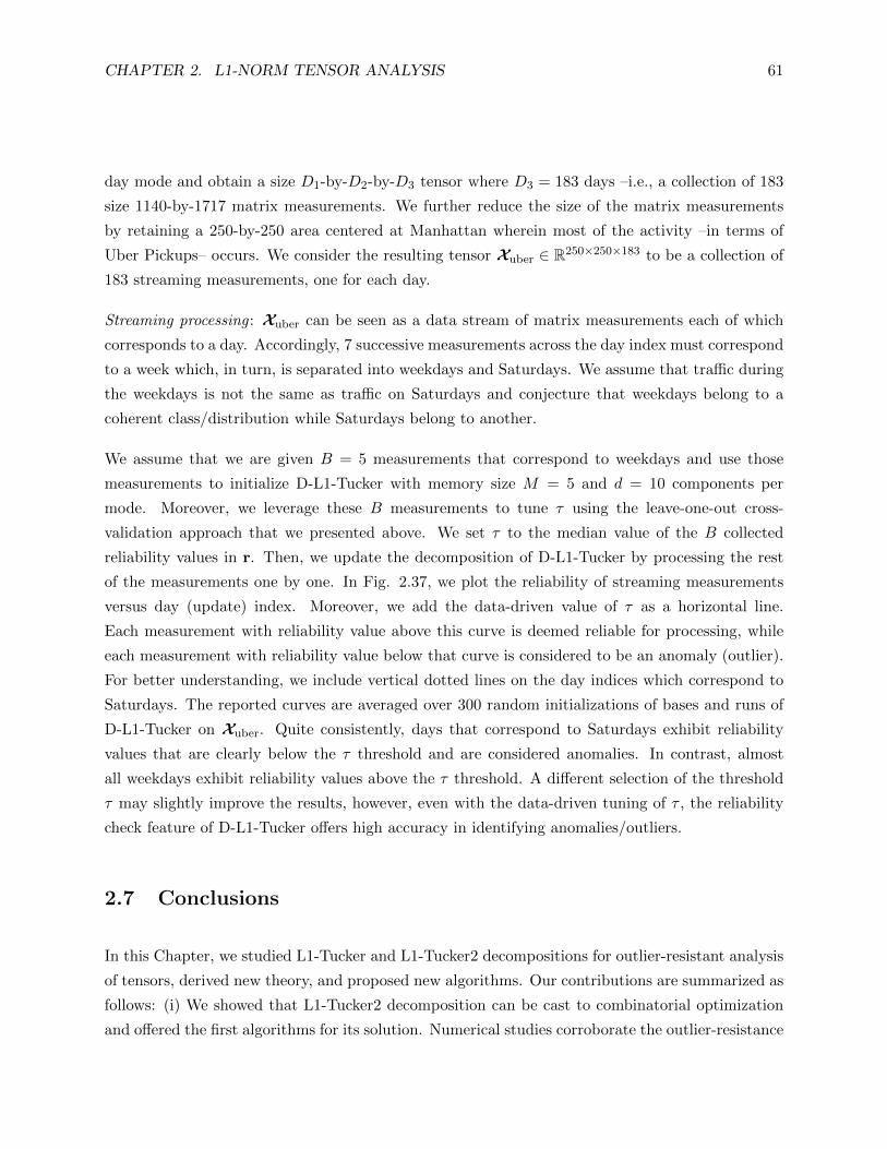
CHAPTER 2. L1-NORM TENSOR ANALYSIS 61
day mode and obtain a size D1-by-D2-by-D3 tensor where D3 = 183 days –i.e., a collection of 183
size 1140-by-1717 matrix measurements. We further reduce the size of the matrix measurements
by retaining a 250-by-250 area centered at Manhattan wherein most of the activity –in terms of
Uber Pickups– occurs. We consider the resulting tensor Xuber ∈ R250×250×183 to be a collection of
183 streaming measurements, one for each day.
Streaming processing : Xuber can be seen as a data stream of matrix measurements each of which
corresponds to a day. Accordingly, 7 successive measurements across the day index must correspond
to a week which, in turn, is separated into weekdays and Saturdays. We assume that traffic during
the weekdays is not the same as traffic on Saturdays and conjecture that weekdays belong to a
coherent class/distribution while Saturdays belong to another.
We assume that we are given B = 5 measurements that correspond to weekdays and use those
measurements to initialize D-L1-Tucker with memory size M = 5 and d = 10 components per
mode. Moreover, we leverage these B measurements to tune τ using the leave-one-out cross-
validation approach that we presented above. We set τ to the median value of the B collected
reliability values in r. Then, we update the decomposition of D-L1-Tucker by processing the rest
of the measurements one by one. In Fig. 2.37, we plot the reliability of streaming measurements
versus day (update) index. Moreover, we add the data-driven value of τ as a horizontal line.
Each measurement with reliability value above this curve is deemed reliable for processing, while
each measurement with reliability value below that curve is considered to be an anomaly (outlier).
For better understanding, we include vertical dotted lines on the day indices which correspond to
Saturdays. The reported curves are averaged over 300 random initializations of bases and runs of
D-L1-Tucker on Xuber. Quite consistently, days that correspond to Saturdays exhibit reliability
values that are clearly below the τ threshold and are considered anomalies. In contrast, almost
all weekdays exhibit reliability values above the τ threshold. A different selection of the threshold
τ may slightly improve the results, however, even with the data-driven tuning of τ , the reliability
check feature of D-L1-Tucker offers high accuracy in identifying anomalies/outliers.
2.7 Conclusions
In this Chapter, we studied L1-Tucker and L1-Tucker2 decompositions for outlier-resistant analysis
of tensors, derived new theory, and proposed new algorithms. Our contributions are summarized as
follows: (i) We showed that L1-Tucker2 decomposition can be cast to combinatorial optimization
and offered the first algorithms for its solution. Numerical studies corroborate the outlier-resistance

CHAPTER 2. L1-NORM TENSOR ANALYSIS 62
20 40 60 80 100 120 140 160 180
Day index
0.4
0.5
0.6
0.7
0.8
0.9
Rel
iabi
lity
Data-driven Saturday
Figure 2.37. Online anomaly detection. B = 5, M = 5, d = 10, 300 realizations, data-driven τ .
of L1-Tucker2 against standard counterparts. (ii) We presented L1-Tucker and L1-Tucker2 decom-
position of general-order tensors and proposed two new algorithmic frameworks for their solution,
L1-HOSVD and L1-HOOI. The presented methods are accompanied by formal convergence and
complexity analyses. Our numerical studies on data restoration and classification demonstrate
that, in contrast to standard Tucker, L1-Tucker decomposition exhibits sturdy resistance against
corruptions among the processed data. (iii) We presented D-L1-Tucker: an algorithm for dynamic
and outlier-resistant Tucker analysis of tensor data. Our experimental studies on real and synthetic
datasets corroborate that the proposed method (1) attains high bases estimation performance, (2)
suppresses outliers, and (3) adapts to changes of the nominal subspaces.
Chapter 3
Lp-quasinorm Principal-Component
Analysis
3.1 Introduction
Principal-Component Analysis (PCA) is a fundamental method for data analysis, machine learn-
ing, and pattern recognition [114]. PCA finds applications in virtually every field of science and
engineering. Computer vision, robotics, neuroscience, signal processing, and medicine are just a few
applications in which PCA has successfully been employed. PCA is typically used for dimensionality
reduction, denoising, classification, clustering, and feature extraction, among others.
PCA is typically formulated as a L2-norm error minimization, or, equivalently, a L2-norm projection
maximization problem. Mathematically, for given matrix X of size D-by-N , PCA seeks a collection
of K D-dimensional unit-norm vectors arranged as columns of a subspace basis matrix Q that
minimizes ‖X−QQ>X‖2F , or equivalently, maximizes ‖X>Q‖2F , where the squared Frobenius/L2
norm ‖·‖2F returns the sum of the squared entries of its argument. The solution to PCA is typically
computed by Singular-Value Decomposition (SVD) of X [115]. Considering that X ∈ RD×N has
rank ρ ≤ D,N and admits SVD X = UΣρ×ρV> such that U>U = V>V = Iρ, Σ = diag(σ), and
[σ]1 ≥ [σ]2 ≥ . . . ≥ [σ]ρ > 0, then the solution to PCA is given by the K left-hand signular-valued
singular vectors of X –i.e., Q = [U]:,1:K solves PCA of X.
Despite its documented success, PCA is known to exhibit severe sensitivity against outliers within
the processed data [47, 48]. Outliers are high-magnitude/peripheral data points that lie far away
63

CHAPTER 3. LP-QUASINORM PRINCIPAL-COMPONENT ANALYSIS 64
from the nominal data subspace and commonly appear in modern datasets –e.g., due to data
storage/transfer errors, faulty sensors, or deliberate data contamination in adversarial environments
[116]. The outlier-sensitivity of PCA is often attributed to its L2-norm-based formulation which
places squared emphasis to each data point, thus promoting the impact of outliers. Accordingly,
applications that rely on PCA are severely affected when outliers exist in the processed data [117].
To counteract the impact of outliers, researchers have proposed an array of “robust” PCA formula-
tions [117, 118]. For instance, one approach considers a L1-norm based residual-error minimization
formulation the (approximate) solution to which is computed by means of alternating-optimization
[119]. Similarly, the authors of [120] study low-rank approximation of a matrix by a residual error
minimization formulation based on the Lp-norm for p ≥ 1. The author of [121] considers the same
problem and presents practical algorithms specifically for p = 1 or p =∞.
A more straightforward approach considers the projection maximization PCA formulation and
replaces the outlier-sensitive L2-norm by the more robust L1-norm (special case of Lp-PCA for
p = 1). This results in the popular L1-norm PCA (L1-PCA) formulation. L1-PCA was solved
exactly in [53, 54]. Efficient [58, 73], adaptive [77], incremental [122], stochastic [123], and complex-
valued data [124, 125] solvers have also been proposed. L1-PCA has been successfully employed
in an array of applications [55–57, 126, 127] where it has been documented that it attains similar
performance to PCA when the processed data are nominal/clean while it exhibits strong resistance
against outliers. L1-norm formulations have recently been proposed for robust tensor analysis –e.g.,
L1-Tucker [59, 63] and L1-Rescal [128]). Similar to L1-PCA, L1-Tucker and L1-Rescal exhibited
significant robustness against data corruptions.
Interestingly, Lp-norm formulations and algorithms have been studied for popular problems other
than PCA. For example, the authors of [129] considered the popular Independent Component
Analysis (ICA) problem and present a variant formulated based on the Lp-norm. Authors in
[130, 131] have studied Linear Discriminant Analysis (LDA) formulations based on the Lp-norm.
Block Principal-Component Analysis has also been studied from the scope of Lp-norm formulations
[132]. Finally, Lp-norm based constraints have been considered for infrared small target detection
[133].
In this work, we study the problem of projection maximization Lp-quasinorm (p ≤ 1) Principal-
Component Analysis, the theoretical foundations of which, remain largely unexplored to date.
This problem was originally studied in [134] where the author considered any general value of p > 0
and presented algorithms for the solution to Lp-PCA. However, the presented algorithms are only
convergent for the special case that p ≥ 1. Moreover, the same problem was also studied in [135]

CHAPTER 3. LP-QUASINORM PRINCIPAL-COMPONENT ANALYSIS 65
where a Grassmann manifold optimization algorithm was proposed for the solution to Lp-PCA.
This algorithm is guaranteed to converge to a locally optimal solution. For p ≤ 1, to the best of
our knowledge, to date there exists no algorithm for the exact solution to Lp-PCA. With this work,
we strive to fill this void.
In this Chapter, we study the theoretical foundations of Lp-quasinorm PCA and propose algorithms
for its solution. Specifically, our contributions are as follows:
Contribution i. We show that, for K = 1, Lp-PCA can always be solved exactly by means of
combinatorial optimization and offer the first algorithms for its solution.
Contribution ii. For the special case of non-negative data, we show that a combinatorial search
can be evaded and finding the dominant Lp-PC of a matrix simplifies to a convex
problem.
Contribution iii. We show that, for general K ≥ 1, the solution to Lp-PCA can also be pursued
by combinatorial optimization and present a novel near-exact algorithm.
Contribution iv. We propose a refining strategy, that, in some cases, can further enhance a near-
exact solution.
The rest of this Chapter is organized as follows. In Section 3.2, we introduce the problem statement.
In Section 3.3, we present exact algorithms for Lp-PCA (K = 1). In Section 3.4, we show that, for
non-negative data, computing the dominant Lp-norm component simplifies to a convex problem.
In Section 3.5, we present a near-exact algorithm for jointly computing multiple Lp-norm PCs. In
Section 3.6, we propose a solution-refinement strategy that, in some cases, can further enhance a
near exact solution. Section 3.7 holds numerical experimental studies on synthetic and real-world
medical data. Concluding remarks are drawn in Section 3.8.
The contributions presented in this Chapter have also been presented in [136–138].
3.2 Problem Statement
Before we present the problem statement, we introduce notation that will facilitate the presentation
of this Chapter.

CHAPTER 3. LP-QUASINORM PRINCIPAL-COMPONENT ANALYSIS 66
Vectors and matrices are denoted by lower-case and upper-case bold letters –i.e., a and A, respec-
tively. SD×K = Q ∈ RD×K : Q>Q = IK is the Stiefel manifold of all rank-K orthonormal
matrices in RD. The set BD×K := Q ∈ RD×K : ‖Q‖2 ≤ 1 is the convex hull of SD×K . For the
special case K = 1, BD×K boils down to the unit-radius hyperball. For any A ∈ RN×K and p > 0,
‖A‖p = ‖vec(A)‖p = (∑N
n=1
∑Kk=1 |[A]n,k|p)
1p . For p ≥ 1, ‖ · ‖p is a proper norm function that, for
any x ∈ RD, y ∈ RD, and α ∈ R, satisfies (i) ‖αx‖p = |a|‖x‖p, (ii) ‖x‖p = 0 implies that x = 0D,
and (iii) ‖x + y‖p ≤ ‖x‖p + ‖y‖p. In contrast, for p ≤ 1, ‖ · ‖p is a quasinorm function and satisfies
(i) and (ii) while (iii) is substituted by ‖x+y‖p ≤ C(‖x‖p+‖y‖p), where it holds that the constant
C = 21−pp > 0 [139]. sgn (·) returns the signs of its input argument –i.e, sgn (α) = +1 if α > 0 and
sgn (α) = −1 if α < 0. Without loss of generality, we set sgn (α) = +1 if α = 0. For any positive
integer N , [N ] = 1, 2, . . . , N. “ ” denotes the element-wise multiplication operation.
We consider a collection of N vector measurements arranged as columns of X = [x1,x2, . . . ,xN ] ∈RD×N . The problem of interest is Lp-quasinorm Principal-Component Analysis (Lp-PCA) of X, for
any p ≤ 1, –i.e., we seek a column-wise orthonormal matrix corresponding to a lower dimensional
signal subspace such that the Lp-quasinorm derived projection variance is maximized. Mathemat-
ically, for any K < rank(X) ≤ minD,N, Lp-PCA is formulated as
max.Q∈SD×K
∥∥∥X>Q∥∥∥pp. (3.1)
A solution to Lp-PCA exists only for the very special case that p = 1. For the area of interest
–general values of p ≤ 1– the solution to Lp-PCA remains unknown to date.
The problem of finding the exact solution to Lp-PCA in (3.1) (or, nearly-exact in a few cases), is
the main focus of this work. Before we commence our developments, we present Lemma 3.1 which
states that, without loss of generality (w.l.o.g.), it suffices to solve (3.1) for a full row rank matrix.
Lemma 3.1. X has rank-ρ and admits SVD X = UΣV> with U ∈ SD×ρ, V ∈ SN×ρ, and
Σ = diag(σ) ∈ Rρ×ρ. Let Y = ΣV>. If Aopt solves max.A∈Sρ×K ‖Y>A‖pp, then Qopt = UAopt
solves (3.1).
By Lemma 3.1, we henceforth consider that X has full row rank –i.e., ρ = D ≤ N .

CHAPTER 3. LP-QUASINORM PRINCIPAL-COMPONENT ANALYSIS 67
(a) p = 2 (b) p = 1 (c) p = 0.5
Figure 3.1. Metric surface of ‖X>q‖pp for arbitrary X ∈ R2×5 and p ∈ 2, 1, 0.5.
3.3 Contribution 1: The Lp-quasinorm Principal-Component
First, we steer our focus on the special case K = 1 in which the problem of interest simplifies to
max.q∈SD×1
∥∥∥X>q∥∥∥pp. (3.2)
For context, we illustrate the cost function of (3.2) for arbitrary X ∈ R2×5 over the unit-radius
hyperball and for p = 2, p = 1, and p = 0.5, in Fig. 3.1a, Fig. 3.1b, and Fig. 3.1c, respectively.
For K = 1, the Stiefel manifold simplifies to the D-dimensional unit-radius hypersphere which
comprises all D-dimensional unit-norm vectors.
Next, we present Lemma 3.2.
Lemma 3.2. For any X ∈ RD×N , solving (3.2) is equivalent to solving max.q∈BD×1‖X>q‖pp.
Lemma 3.2 states that the solution to Lp-PCA can equivalently be pursued over the closed unit-
radius D-dimensional hyperball. Next, we consider b = ±1N and define the set
C(b) = q ∈ BD×1 : sgn(X>q
)= b. (3.3)
In practice, C(b) is a subset of the unit-radius hyperball. Some instances of b will be such that
C(b) = ∅. Further, every distinct b uniquely identifies a subset of the hyperball in accordance with
the following Lemma 3.3.
Lemma 3.3. For every b,b′ ∈ ±1N such that b 6= b′, it holds that C(b) ∩ C(b′) = ∅.
All sets C(b) formed by b when it scans the finite-size set ±1N are, in practice, a partition of

CHAPTER 3. LP-QUASINORM PRINCIPAL-COMPONENT ANALYSIS 68
(a) b = [−1, 1,−1, 1,−1]> (b) b = [1,−1, 1,−1, 1]>
Figure 3.2. Metric surface of ‖X>q‖pp for p = 0.5 and arbitrary X ∈ R2×5 when q scans C(b) forfixed b.
Input: X ∈ RD×N , b ∈ ±1N , p ≤ 1Output: q ∈ RD
Y = X ∗ diag (b ) ;cvx beg inv a r i a b l e q (D)maximize (sum( pow p (Y’ ∗ q , p ) )q ’ ∗ q <= 1Y’ ∗ q >= 0cvx end
Figure 3.3. CVX code (Matlab) for the solution to (3.4).
the hyperball which corresponds to the data matrix X as shown in the following Lemma 3.4.
Lemma 3.4. It holds that BD×1 =⋃
b∈±1N C(b).
By Lemma 3.2 and Lemma 3.4, maxq∈BD×1
∥∥X>q∥∥pp
= maxb∈±1N maxq∈C(b)
∥∥X>q∥∥pp. Accorid-
ngly, the solution to Lp-PCA can be pursued by combinatorial search over ±1N –i.e., by sepa-
rately solving
max.q∈C(b)
∥∥∥X>q∥∥∥pp
(3.4)
for every b ∈ ±1N .
Next, we show that the solution to (3.4) exists and can be found exactly, in accordance with the
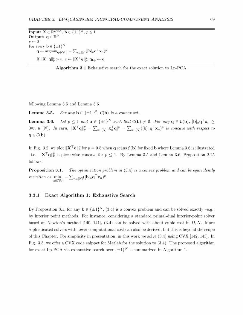
CHAPTER 3. LP-QUASINORM PRINCIPAL-COMPONENT ANALYSIS 69
Input: X ∈ RD×N , b ∈ ±1N , p ≤ 1Output: q ∈ RD
v ← 0For every b ∈ ±1N
q← argminq∈C(b) −∑
n∈[N ]([b]nq>xn)p
If ‖X>q‖pp > v, v ← ‖X>q‖pp, qLp ← q
Algorithm 3.1 Exhaustive search for the exact solution to Lp-PCA.
following Lemma 3.5 and Lemma 3.6.
Lemma 3.5. For any b ∈ ±1N , C(b) is a convex set.
Lemma 3.6. Let p ≤ 1 and b ∈ ±1N such that C(b) 6= ∅. For any q ∈ C(b), [b]nq>xn ≥
0∀n ∈ [N ]. In turn, ‖X>q‖pp =∑
n∈[N ] |x>nq|p =∑
n∈[N ]([b]nq>xn)p is concave with respect to
q ∈ C(b).
In Fig. 3.2, we plot ‖X>q‖pp for p = 0.5 when q scans C(b) for fixed b where Lemma 3.6 is illustrated
–i.e., ‖X>q‖pp is piece-wise concave for p ≤ 1. By Lemma 3.5 and Lemma 3.6, Proposition 2.25
follows.
Proposition 3.1. The optimization problem in (3.4) is a convex problem and can be equivalently
rewritten as min.q∈C(b)
−∑
n∈[N ]([b]nq>xn)p.
3.3.1 Exact Algorithm 1: Exhaustive Search
By Proposition 3.1, for any b ∈ ±1N , (3.4) is a convex problem and can be solved exactly –e.g.,
by interior point methods. For instance, considering a standard primal-dual interior-point solver
based on Newton’s method [140, 141], (3.4) can be solved with about cubic cost in D,N . More
sophisticated solvers with lower computational cost can also be derived, but this is beyond the scope
of this Chapter. For simplicity in presentation, in this work we solve (3.4) using CVX [142, 143]. In
Fig. 3.3, we offer a CVX code snippet for Matlab for the solution to (3.4). The proposed algorithm
for exact Lp-PCA via exhaustive search over ±1N is summarized in Algorithm 1.
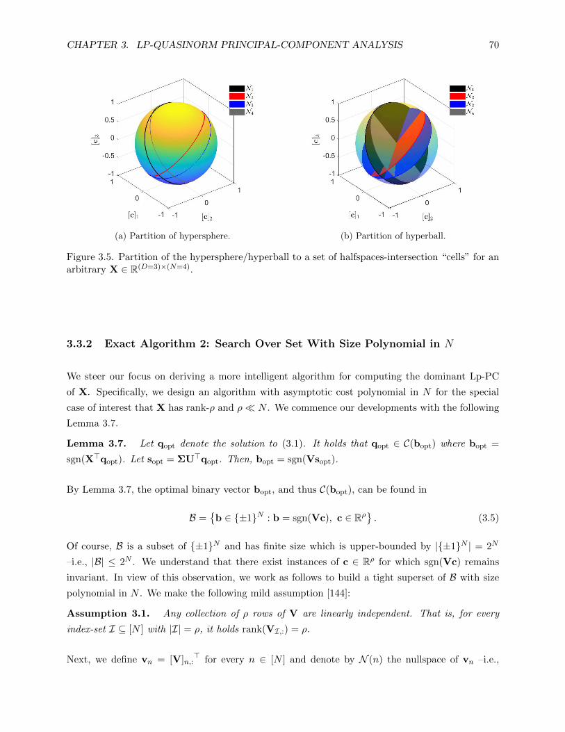
CHAPTER 3. LP-QUASINORM PRINCIPAL-COMPONENT ANALYSIS 70
(a) Partition of hypersphere. (b) Partition of hyperball.
Figure 3.5. Partition of the hypersphere/hyperball to a set of halfspaces-intersection “cells” for anarbitrary X ∈ R(D=3)×(N=4).
3.3.2 Exact Algorithm 2: Search Over Set With Size Polynomial in N
We steer our focus on deriving a more intelligent algorithm for computing the dominant Lp-PC
of X. Specifically, we design an algorithm with asymptotic cost polynomial in N for the special
case of interest that X has rank-ρ and ρ N . We commence our developments with the following
Lemma 3.7.
Lemma 3.7. Let qopt denote the solution to (3.1). It holds that qopt ∈ C(bopt) where bopt =
sgn(X>qopt). Let sopt = ΣU>qopt. Then, bopt = sgn(Vsopt).
By Lemma 3.7, the optimal binary vector bopt, and thus C(bopt), can be found in
B =b ∈ ±1N : b = sgn(Vc), c ∈ Rρ
. (3.5)
Of course, B is a subset of ±1N and has finite size which is upper-bounded by |±1N | = 2N
–i.e., |B| ≤ 2N . We understand that there exist instances of c ∈ Rρ for which sgn(Vc) remains
invariant. In view of this observation, we work as follows to build a tight superset of B with size
polynomial in N . We make the following mild assumption [144]:
Assumption 3.1. Any collection of ρ rows of V are linearly independent. That is, for every
index-set I ⊆ [N ] with |I| = ρ, it holds rank(VI,:) = ρ.
Next, we define vn = [V]n,:> for every n ∈ [N ] and denote by N (n) the nullspace of vn –i.e.,

CHAPTER 3. LP-QUASINORM PRINCIPAL-COMPONENT ANALYSIS 71
Input: X ∈ RD×N , p ≤ 1Output: qopt ∈ RD
v ← 0(U,Σρ×ρ ,V
>)← svd(X)For every J ⊂ [N ], |J | = ρ− 1
Build BJ in (3.16)
For every b ∈ BJq← arg minq∈C(b)−
∑n∈[N ]([b]nx>n q)p
If ‖X>q‖pp > v, v ← ‖X>q‖pp,qopt ← q
Algorithm 3.2 Exact Lp-PCA via search over polynomial (in N) size set.
N (n) = span(Iρ − vnv>n ). We observe that, for every c ∈ N (n), the non-negative angle between
c and vn, φ(c,vn) = π2 and, accordingly, c>vn = ‖c‖2‖vn‖2 cos (φ(c,vn)) = 0. This implies that
N (n) divides Rρ into two non-overlapping hyperplanes (halfspaces) H(n)+ and H(n)− such that
[100]
H(n)+ =
c ∈ Rρ : sgn(c>vn) = +1, (3.6)
H(n)− =
c ∈ Rρ : sgn(c>vn) = −1. (3.7)
By the definition of sgn (·), H(n)+ is an open set including the boundary N (n) while H(n)− is an
open set that does not include the boundary N (n). Accordingly, it holds that H(n)+ ∩H(n)− = ∅.For example, consider some ρ ≥ 3 and indices m < s ∈ [N ]. N (m) and N (s) divide Rρ in the
halfspaces H(m)+,H(m)− and H(s)+,H(s)−, respectively. By Assumption 3.1, each of the two
halfspaces defined by N (i) for some i ∈ m, s will intersect with each of two halfspaces defined by
N (j), j ∈ m, s \ i. These intersections result in the four halfspaces-intersection “cells”
C1 = H(m)− ∩H(s)−, (3.8)
C2 = H(m)− ∩H(s)+, (3.9)
C3 = H(m)+ ∩H(s)−, (3.10)
C4 = H(m)+ ∩H(s)+. (3.11)
Importantly, for any j ∈ [4] and i ∈ m, s, [sgn(Vc)]i remains the same across Cj –i.e., for
any c ∈ C3, [sgn(Vc)]m = +1 and [sgn(Vc)]s = −1. To better understand how the halfspaces-
intersection “cells” are formed, in Fig. 3.5, we offer a visual illustration for arbitrary matrix
X ∈ R(D=3)×(N=4).

CHAPTER 3. LP-QUASINORM PRINCIPAL-COMPONENT ANALYSIS 72
Next, we generalize the above discussion and consider the arrangement of all N hyperplanes
N (n)∀n ∈ [N ]. These hyperplanes partition Rρ in L non-overlapping cells for some finite L which
depends on ρ and N . Formally, for every l ∈ [L], the l-th halfspaces-intersection cell is defined as
Cl =⋂i∈I+H(i)+
⋂j∈I−
H(j)−, (3.12)
where I+ ⊂ [N ], I− ⊂ [N ], I+ ∩ I− = ∅, and I+ ∪ I− = [N ] [145, 146]. By the above discussions,
every c ∈ Cl lies in the same intersection of halfspaces and yields the same sgn(Vc). It holds
[sgn(Vc)]n = sgn(v>n c) =
+1, n ∈ I+,
−1, n ∈ I−.(3.13)
Thereafter, we define a signature for each cell, bl = sgn(Vc) for some c ∈ Cl. We notice that, for
every (k, l) ∈ [N ]× [N ] such that k 6= l, Ck ∩Cl = ∅ and that⋃l∈[L] Cl = Rρ. By the above analysis,
the set B in (3.5) takes the equivalent form
B =⋃l∈[L]
sgn(Vc) : c ∈ Cl = b1,b2, . . . ,bL. (3.14)
It has been shown [103, 145] that L = 2∑ρ−1
k=0
(N−1k
)≤ 2N with equality attained if and only if
ρ = N . It follows that the cardinality of the signature set B is also L. In the sequel, we rely on
the above discussions and construct a tight superset of B. By Assumption 3.1, for any index-set
J ⊆ [N ] with |J | = ρ− 1 and complementary set J c = [N ] \ J , the halfspaces-intersection
SJ =⋂n∈[J ]
N (n) (3.15)
is a line (one-dimensional subspace) in Rρ. By definition, this line is the verge between all cells
that are jointly bounded by the ρ− 1 hyperlanes. Then, we consider a vector c ∈ Rρ that crosses
the verge SJ (at any point other than 0ρ). By this crossing, the value of [sgn(Vc)]J will change
so that it adjusts to the cell it just entered while the value of [sgn(Vc)]J c will remain invariant.
This follows straightforwardly by the fact that a crossing over SJ can not be simultaneous over a
crossing of any of the hyperplanes corresponding to J c. Accordingly, for any c ∈ SJ \ 0ρ, the set
BJ =b ∈ ±1N : [b]J c = [sgn(Vc)]J c
(3.16)
contains all the signatures of all the cells are that are bounded by the verge SJ –i.e., all non-zero

CHAPTER 3. LP-QUASINORM PRINCIPAL-COMPONENT ANALYSIS 73
points c asymptotically close to SJ yield sgn(Vc) that lies in BJ . Moreover, there exists at least
one such verge that bounds it. Therefore, the set
B? =⋃
J⊆[N ] : |J |=ρ−1
BJ (3.17)
includes all cell signatures and, thus, is a superset of B.
Next, we study the size of B? and the computational effort required for forming it. We notice
that for every instance of J , it holds that |BJ | = 2ρ−1, which derives by the sign ambiguity by
the nullspace of each row of V. Moreover, there exist(Nρ−1
)distinct instances of J which implies
that |B?| is upper bounded by 2ρ−1(Nρ−1
). Both B? and B have polynomial size in N . In practice,
for every instance of J , c can be computed by Gram-Schmidt orthogonalization of [V]J ,:> with
cost O(ρ3). Retaining the dominant terms, B? can be computed with serial cost O(Nρ−1) or by(Nρ−1
)parallel processes. The exact Lp-PC of X can be found by a search over B?. The proposed
algorithm for exact Lp-PCA via a search over B? is summarized in Algorithm 2.
In view of the above, the Lp-PC of a matrix can be computed exactly by a search over ±1N
or (more intelligently) by a search over B?. In both cases, multiple instances of (3.4) must be
solved. Accordingly, a discussion on the computational effort required for solving (3.4) is in order.
First, we note that numerous distinct solvers can be developed for solving (3.4) enabling different
performance/complexity trade-offs. For simplicity in presentation and to remain within the scope
of this chapter, we presented a solution to (3.4) via CVX’s [142, 143] standardized algorithms.
For a better understanding with respect to the computational effort required for solving (3.4), we
developed a modified primal-dual Newton’s algorithm the presentation of which is omitted as it
extends well beyond the scope of this chapter: to study the underlying mechanics of Lp-PCA and
develop new theory that enables us to compute the exact solution. The per-iteration cost of this
algorithm is dominated by the inversion of a Jacobian matrix with cost O(N3 +D3) –i.e., cubic in
both the number of features and number of points in X. Letting T denote the number of iterations
required for convergence, the overall complexity becomes O(T (N3 + D3)). In practice, we have
observed that T minD,N. Certainly, more sophisticated algorithms can be designed further
reducing the computational effort required for solving Lp-PCA exactly.

CHAPTER 3. LP-QUASINORM PRINCIPAL-COMPONENT ANALYSIS 74
3.4 Contribution 2: The Dominant Lp-PC of a Non-Negative Ma-
trix
We consider the special case of interest that X has non-negative entries –i.e., for every (i, j) ∈[D] × [N ], [X]i.j ≥ 0. The following Proposition 3.2 states that the Lp-PC of X can be found
exactly without a search.
Proposition 3.2. If X has non-negative entries, then
maxq∈BD×1
‖X>q‖pp = maxq∈C(1N )
‖X>q‖pp. (3.18)
By Proposition 3.2, forming B? is not necessary when X has non-negative entries. Solving (3.4) for
b = 1N suffices for computing the Lp-PC of X.
3.5 Contribution 3: Joint Extraction of Multiple Lp-quasinorm
Principal-Components
We now consider the problem of jointly computing K Lp-PCs of X, for general K > 1. For
readability, we present again the formulation of Lp-PCA
max.Q∈SD×K
∥∥∥X>Q∥∥∥pp. (3.19)
First, similar to the presented theory for K = 1, we notice that the Stiefel manifold can be
partitioned into a finite number of non-overlapping sets. That is, for every B ∈ ±1N×K , we
define
C(B) = Q ∈ SD×K : sgn(X>Q
)= B. (3.20)
Accordingly, w.l.o.g., Lp-PCA in (3.1) can equivalently be written as
max.Q∈⋃
B∈±1N×K C(B)
∥∥∥X>Q∥∥∥pp. (3.21)

CHAPTER 3. LP-QUASINORM PRINCIPAL-COMPONENT ANALYSIS 75
Input: X ∈ RD×N , B ∈ ±1N×K , p ≤ 1Output: Q ∈ RD×K
cvx beg inv a r i a b l e Q(D,K)co s t = 0 ;f o r k = 1 :K
Yk = X ∗ diag (B( : , k ) ) ;c o s t = cos t + sum( pow p (Yk’ ∗ Q( : , k ) , p ) ;Yk’ ∗ Q( : , k ) >= 0
endmaximize ( co s t )norm(Q, 2) <= 1cvx end
Figure 3.7. CVX code (Matlab) for the solution to (3.24).
In view of (3.21), we consider fixed B ∈ ±1N×K and steer our focus on solving
max.Q∈C(B)
∥∥∥X>Q∥∥∥pp. (3.22)
By Lemma 3.6 and the fact that ‖X>Q‖pp =∑
k∈[K] ‖X>qk‖pp for any Q ∈ RD×K , we present the
following Lemma 3.8.
Lemma 3.8. The cost function ‖X>Q‖pp =∑
k∈[K] ‖X>qk‖pp =∑
n∈[N ]
∑k∈[K](x
>nqk[B]n,k) is
concave with respect to Q ∈ C(B).
Lemma 3.8 derives straightforwardly by applying Lemma 3.6 K times. Even though the cost
function of (3.22) is concave with respect to the maximizing argument, the optimization problem
itself is not convex nor concave because of the Stiefel manifold constraint (orthogonality constraints)
and, accordingly, solving (3.22) is not a trivial task. Similar to standard practice in the literature
[147, 148], we consider a convex relaxation formulation of (3.22) by substituting the Stiefel manifold
constraint –i.e., Q ∈ SD×K– by ‖Q‖2 = σmax(Q) ≤ 1.1 The set Q ∈ RD×K : ‖Q‖2 ≤ 1 is the
convex hull of SD×K –i.e., the smallest convex set which includes it [149].
Formally, we define the set
C(B) = Q ∈ RD×K : ‖Q‖2 ≤ 1, sgn(X>Q
)= B (3.23)
1For any matrix A, σmax(A) denotes the maximum singular value of A.

CHAPTER 3. LP-QUASINORM PRINCIPAL-COMPONENT ANALYSIS 76
and consider a convex relaxation formulation of (3.22) of the form
max.Q∈C(B)
∥∥∥X>Q∥∥∥pp. (3.24)
We have already established that the cost function of (3.22) (and, thus, (3.24)) is concave with
respect to the maximizing argument. The following Lemma 3.9 states that the set C(B) is a convex
set.
Lemma 3.9. For any B ∈ ±1N×K , C(B) is a convex set.
By Lemma 3.8 and Lemma 3.9, the following Proposition 3.3 naturally follows.
Proposition 3.3. The optimization problem in (3.24) is a convex problem and can be equivalently
rewritten as min.Q∈C(B)
−∑
n∈[N ]
∑k∈[K]([B]n,kx
>nqk)
p.
For simplicity, in this work we solve (3.24) with CVX [142, 143]. In Fig. 3.7, we offer a CVX
code snippet for Matlab for the solution to (3.24). In the sequel, we discuss how solving (3.24),
for a fixed B, can be leveraged for deriving a solution to the original problem of interest (3.1) (or,
(3.21)).
A straightforward yet naive approach would be to solve (3.24) for every B ∈ ±1N×K (exhaustive
search) and retain the solution that attains the highest metric. While this approach computes the
exact solution to
max.Q∈RD×K :‖Q‖2≤1
∥∥∥X>Q∥∥∥pp, (3.25)
an exhaustive search is not necessary in accordance with the following Lemma 3.10
Lemma 3.10. Let Qopt be the exact solution to maxQ∈C(B) maxB∈±1N×K ‖X>Q‖pp (equivalently
(3.25)). Bopt = sgn(X>Qopt) is such that, for every k ∈ [K], [Bopt]:,k ∈ B?.
By Lemma 3.10, the exact solution to (3.25) can be computed by a search over the set
B?,K = B ∈ ±1N×K : [B]:,k ∈ B?∀k ∈ [K]. (3.26)
In practice, B?,K is the K-fold Cartesian product of B?. Moreover, it holds that B?,K ⊆ ±1N×K
and that |B?,K | = |B?|K ≤ |±1N×K |. In view of this discussion, we propose to solve (3.24) for
every B ∈ B?,K . The proposed algorithm the solving (3.25) is summarized in Algorithm 3.

CHAPTER 3. LP-QUASINORM PRINCIPAL-COMPONENT ANALYSIS 77
Input: X ∈ RD×N , K, p ≤ 1Output: Qopt ∈ RD
v ← 0For every B ∈ B?,K
Q← arg minQ∈C(B)−∑
n∈[N ]
∑k∈[K]([B]n,kx>n qk)p
If ‖X>Q‖pp > v, v ← ‖X>Q‖pp, Qopt ← Q
Algorithm 3.3 Multiple Lp-PCs (convex relaxation) via search over polynomial (in N) size set.
Formally, by Algorithm 3 we obtain the exact solution to (3.25) by solving
maxQ∈C(B)
maxB∈B?,K
‖X>Q‖pp. (3.27)
Let Qopt denote the exact solution to (3.27). We distinguish two cases for Qopt: (i) Qopt ∈ SD×Kand (ii) Qopt /∈ SD×K . Then, we present the following Proposition 3.4
Proposition 3.4. If Qopt ∈ SD×K , then it solves Lp-PCA in (3.1) exactly.
Proposition 3.4 states that when the solution of the convex relaxation formulation is in the Stiefel
manifold, then it is also a solution to the original Lp-PCA formulation. Our numerical studies have
shown that this is often the case. In the sequel, we propose an algorithm for computing a solution
in the Stiefel manifold when Qopt /∈ SD×K .
3.6 Contribution 4: Stiefel Manifold Solution Refinement
In this Section, we propose a method for computing a solution to the original problem in (3.1) for
the special case that Qopt /∈ SD×K .
In this case, the most straightforward approach would be to refine Qopt by solving
arg minQ∈SD×K
‖Q− Qopt‖2F . (3.28)
This problem admits an exact solution by means of the Procrustes Theorem. Our numerical studies
have shown that, although simple, this approach is inferior with respect to the Lp-PCA metric,
when compared with the more sophisticated approach that we propose next as follows.
Even if Qopt /∈ SD×K , it provides valuable information about the solution to (3.1). First, we

CHAPTER 3. LP-QUASINORM PRINCIPAL-COMPONENT ANALYSIS 78
understand that v = ‖X>Qopt‖pp serves as an upper-bound of the maximum attainable metric of
the cost function of (3.1). That is, if we denote by Qopt the exact solution to (3.1), then it always
holds that ‖X>Qopt‖pp ≤ ‖X>Qopt‖pp. Moreover, it is reasonable to expect that Qopt can exhibit
low Euclidean distance from Qopt when we consider that the metric surface of the cost function
is concave over C(Bopt), where Bopt = sgn(X>Qopt). Accordingly, we propose to use Qopt as an
“anchor” and search over an area near it while at the same time trying to maximize the metric
of interest. To this end, we propose an iterative algorithm for computing a solution in the Stiefel
manifold by leveraging Qopt as follows. First, we initialize Q1 = Qopt. Then, at every iteration
i ≥ 1, we update
Qi+1 = arg maxQ∈C(Bopt)
1
v
∑n∈[N ]
∑k∈[K]
([B]n,kx>nqk)
p + τTr(Q>Qi), (3.29)
where τ > 0 is a regularization coefficient that promotes orthogonality among the columns of Q.
For any fixed iteration index i, the above problem is, of course, a convex problem. Moreover, at
every iteration the compound metric in (3.29) is increasing. At the same time, the compound metric
is upper bounded. Accordingly, convergence is guaranteed. Importantly, for an appropriate choice
of τ , the term τTr(Q>Qi) will enforce the Stiefel manifold constraint. Interestingly, the proposed
iteration in (3.29) is similar, in formulation, with the general form of proximal algorithms [150],
a special class of optimization algorithms. Furthermore, in view of (3.29), we consider a parallel
stream of matrices each of which are guaranteed to be in the Stiefel manifold, independently of the
choice of τ . That is, at every iteration index i ≥ 1, we compute Wi = arg minW∈SD×K ‖W−Qi‖2F .
Next, we evaluate the performance of the proposed iteration in(3.29) by evaluating the Lp-PCA
metric attained by both Qi and Wi, for every i ≥ 1. As measures of success, we consider two
metrics. First, at any fixed iteration index i, we measure the ratio of the Lp-PCA metric attained
by Qi and Wi with respect to the known upper-bound v by computing vi = 1v‖X
>Qi‖pp and
vi = 1v‖X
>Wi‖pp, respectively. Certainly, it holds that vi ≤ 1 and that vi ≤ 1. Second, we measure
the proximity of Qi to the Stiefel manifold by measuring e(i) = 1K ‖Q
>i Qi− IK‖2F . If e(i) = 0 then
Qi is in the Stiefel manifold. Let I denote the converging iteration of (3.29). If vI = 1 and e(I) = 0
at the same time, then the proposed iteration in (3.29) has returned the exact solution to (3.1).
We consider data matrix X ∈ RD×N drawing entries from N (0, 1). We run Algorithm 3 on X and
compute Qopt. If Qopt ∈ SD×K , then we discard it. Otherwise, we give it as input to the iteration
in (3.29) for refining its solution to a solution in the Stiefel manifold. We repeat this process until
we collect 30 realizations of X such that Qopt /∈ SD×K .

CHAPTER 3. LP-QUASINORM PRINCIPAL-COMPONENT ANALYSIS 79
0 2 4 6 8 10 12 14 16Iteration index, i
0.9920
0.9940
0.9960
0.9980
1.0000A
ttain
ed u
pper
-bou
nd r
atio
K 2K K (parallel stream) 2K (parallel stream)
(a) Attained upper-bound ratio vs iteration index.
0 2 4 6 8 10 12 14 16Iteration index, i
0
0.1
0.2
0.3
0.4
0.5 K 2K
(b) Proximity to Stiefel manifold vs iteration index.
Figure 3.9. Evaluation of the proposed iteration in (3.29) for p = 1, D = 3, N = 5, and K = 2.Reported curve-values are averages over 30 realizations of data.
0 2 4 6 8 10 12 14 16Iteration index, i
0.9920
0.9940
0.9960
0.9980
1.0000
Atta
ined
upp
er-b
ound
rat
io
K 2K K (parallel stream) 2K (parallel stream)
(a) Attained upper-bound ratio vs iteration index.
0 2 4 6 8 10 12 14 16Iteration index, i
0
0.1
0.2
0.3
0.4
0.5 K 2K
(b) Proximity to Stiefel manifold vs iteration index.
Figure 3.10. Evaluation of the proposed iteration in (3.29) for p = 0.90, D = 3, N = 5, and K = 2.Reported curve-values are averages over 30 realizations of data.
First, we set D = 3, N = 5, K = 2, and p = 1. In Fig. 3.9a and Fig. 3.9b, we plot (vi,vi) and e(i),
respectively, for τ = K and τ = 2K. The reported performances are averages over 30 realizations.
We observe that both streams of matrices attain the maximum attainable metric across the board
and, at the converging iteration I, both QI and WI are in the Stiefel manifold –i.e., the solution
is exact. Next, we repeat the above study, this time for p = 0.9. We present the performance
curves in Fig. 3.10a and Fig. 3.10b, computed again over 30 realizations. We notice that vi ≥ vi
for every iteration index. Specifically, in early iterations the matrices of the original stream offer
slightly higher metric compared to the matrices of the parallel stream. However, upon convergence,
the matrices of the two streams coincide and converge to the same metric. We repeat the above
experiment, this time for p = 0.75. We illustrate the average performances in Fig. 3.11a and Fig.
3.11b. The observations we make are the same as above.
Thereafter, we adjust the parameter configuration as follows. We set D = 4, N = 5, K = 3, and
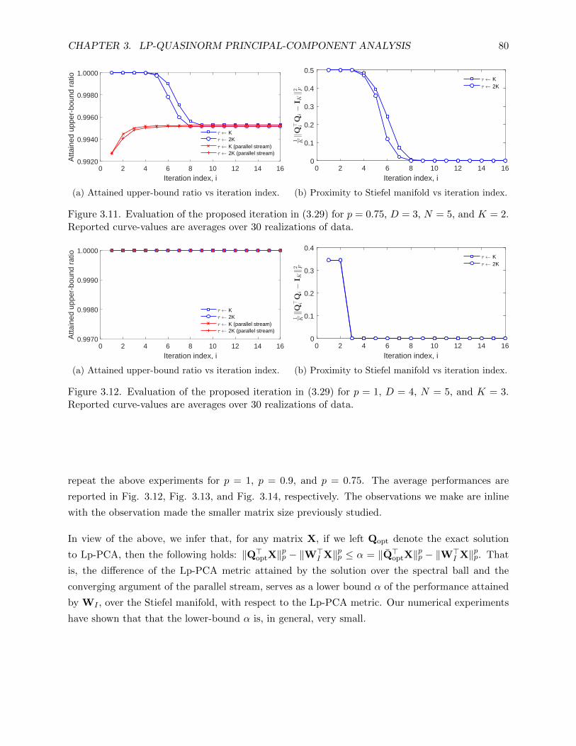
CHAPTER 3. LP-QUASINORM PRINCIPAL-COMPONENT ANALYSIS 80
0 2 4 6 8 10 12 14 16Iteration index, i
0.9920
0.9940
0.9960
0.9980
1.0000A
ttain
ed u
pper
-bou
nd r
atio
K 2K K (parallel stream) 2K (parallel stream)
(a) Attained upper-bound ratio vs iteration index.
0 2 4 6 8 10 12 14 16Iteration index, i
0
0.1
0.2
0.3
0.4
0.5 K 2K
(b) Proximity to Stiefel manifold vs iteration index.
Figure 3.11. Evaluation of the proposed iteration in (3.29) for p = 0.75, D = 3, N = 5, and K = 2.Reported curve-values are averages over 30 realizations of data.
0 2 4 6 8 10 12 14 16Iteration index, i
0.9970
0.9980
0.9990
1.0000
Atta
ined
upp
er-b
ound
rat
io
K 2K K (parallel stream) 2K (parallel stream)
(a) Attained upper-bound ratio vs iteration index.
0 2 4 6 8 10 12 14 16Iteration index, i
0
0.1
0.2
0.3
0.4 K 2K
(b) Proximity to Stiefel manifold vs iteration index.
Figure 3.12. Evaluation of the proposed iteration in (3.29) for p = 1, D = 4, N = 5, and K = 3.Reported curve-values are averages over 30 realizations of data.
repeat the above experiments for p = 1, p = 0.9, and p = 0.75. The average performances are
reported in Fig. 3.12, Fig. 3.13, and Fig. 3.14, respectively. The observations we make are inline
with the observation made the smaller matrix size previously studied.
In view of the above, we infer that, for any matrix X, if we left Qopt denote the exact solution
to Lp-PCA, then the following holds: ‖Q>optX‖pp − ‖W>
I X‖pp ≤ α = ‖Q>optX‖pp − ‖W>
I X‖pp. That
is, the difference of the Lp-PCA metric attained by the solution over the spectral ball and the
converging argument of the parallel stream, serves as a lower bound α of the performance attained
by WI , over the Stiefel manifold, with respect to the Lp-PCA metric. Our numerical experiments
have shown that that the lower-bound α is, in general, very small.

CHAPTER 3. LP-QUASINORM PRINCIPAL-COMPONENT ANALYSIS 81
0 2 4 6 8 10 12 14 16Iteration index, i
0.9970
0.9980
0.9990
1.0000A
ttain
ed u
pper
-bou
nd r
atio
K 2K K (parallel stream) 2K (parallel stream)
(a) Attained upper-bound ratio vs iteration index.
0 2 4 6 8 10 12 14 16Iteration index, i
0
0.1
0.2
0.3
0.4 K 2K
(b) Proximity to Stiefel manifold vs iteration index.
Figure 3.13. Evaluation of the proposed iteration in (3.29) for p = 0.90, D = 4, N = 5, and K = 3.Reported curve-values are averages over 30 realizations of data.
0 2 4 6 8 10 12 14 16Iteration index, i
0.9970
0.9980
0.9990
1.0000
Atta
ined
upp
er-b
ound
rat
io
K 2K K (parallel stream) 2K (parallel stream)
(a) Attained upper-bound ratio vs iteration index.
0 2 4 6 8 10 12 14 16Iteration index, i
0
0.1
0.2
0.3
0.4 K 2K
(b) Proximity to Stiefel manifold vs iteration index.
Figure 3.14. Evaluation of the proposed iteration in (3.29) for p = 0.75, D = 4, N = 5, and K = 3.Reported curve-values are averages over 30 realizations of data.
3.7 Numerical Experiments
In this chapter, we set the theoretical foundations for Lp-quasinorm Principal-Component analysis
and proposed algorithms for its solution. The proposed algorithms are of theoretical value –i.e., they
reveal the underlying properties and mechanics of the problem which, in turn, set the foundations
for developing efficient and scalable algorithms. Nonetheless, the development of such algorithms is
beyond the scope of this Chapter. In the sequel, we conduct numerical experiments on rather small-
sized matrices. The purpose of these studies is to demonstrate the merits of Lp-PCA processing.
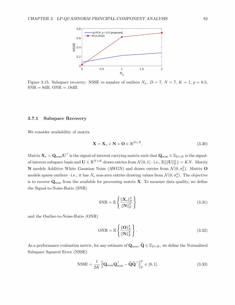
CHAPTER 3. LP-QUASINORM PRINCIPAL-COMPONENT ANALYSIS 82
0 0.5 1 1.5 2N
o
0
0.2
0.4
0.6
0.8
NS
SE
Lp-PCA, p = 0.5 (proposed)PCA (SVD)
Figure 3.15. Subspace recovery: NSSE vs number of outliers No. D = 7, N = 7, K = 1, p = 0.5,SNR = 8dB, ONR = 18dB.
3.7.1 Subspace Recovery
We consider availability of matrix
X = Xs + N + O ∈ RD×N . (3.30)
Matrix Xs = QnomU> is the signal-of-interest carrying matrix such that Qnom ∈ SD×K is the signal-
of-interest subspace basis and U ∈ RN×K draws entries fromN (0, 1) –i.e., E‖U‖2F = KN . Matrix
N models Additive White Gaussian Noise (AWGN) and draws entries from N (0, σ2n). Matrix O
models sparse outliers –i.e., it has No non-zero entries drawing values from N (0, σ2o). The objective
is to recover Qnom from the available for processing matrix X. To measure data quality, we define
the Signal-to-Noise-Ratio (SNR)
SNR = E
‖Xs‖2F‖N‖2F
(3.31)
and the Outlier-to-Noise-Ratio (ONR)
ONR = E
‖O‖2F‖N‖2F
. (3.32)
As a performance evaluation metric, for any estimate of Qnom, Q ∈ SD×K , we define the Normalized
Subspace Squared Error (NSSE)
NSSE =1
2K
∥∥∥QnomQ>nom − QQ>∥∥∥2
F∈ [0, 1]. (3.33)
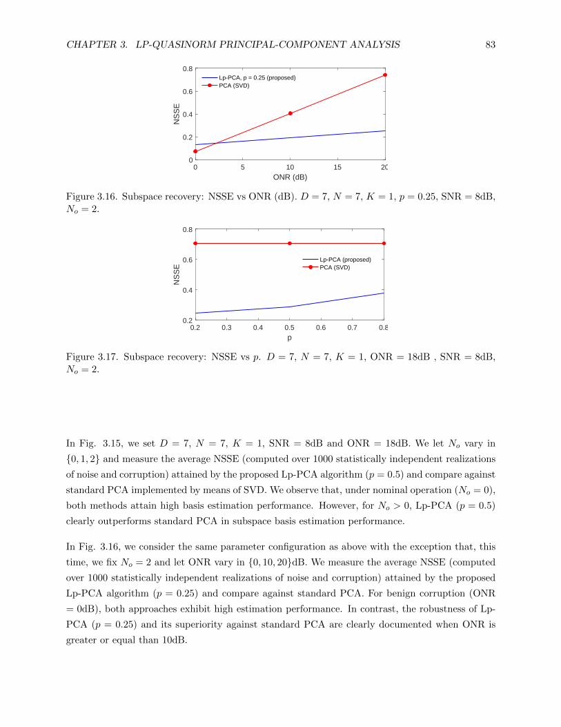
CHAPTER 3. LP-QUASINORM PRINCIPAL-COMPONENT ANALYSIS 83
0 5 10 15 20ONR (dB)
0
0.2
0.4
0.6
0.8
NS
SE
Lp-PCA, p = 0.25 (proposed)PCA (SVD)
Figure 3.16. Subspace recovery: NSSE vs ONR (dB). D = 7, N = 7, K = 1, p = 0.25, SNR = 8dB,No = 2.
0.2 0.3 0.4 0.5 0.6 0.7 0.8p
0.2
0.4
0.6
0.8
NS
SE
Lp-PCA (proposed)PCA (SVD)
Figure 3.17. Subspace recovery: NSSE vs p. D = 7, N = 7, K = 1, ONR = 18dB , SNR = 8dB,No = 2.
In Fig. 3.15, we set D = 7, N = 7, K = 1, SNR = 8dB and ONR = 18dB. We let No vary in
0, 1, 2 and measure the average NSSE (computed over 1000 statistically independent realizations
of noise and corruption) attained by the proposed Lp-PCA algorithm (p = 0.5) and compare against
standard PCA implemented by means of SVD. We observe that, under nominal operation (No = 0),
both methods attain high basis estimation performance. However, for No > 0, Lp-PCA (p = 0.5)
clearly outperforms standard PCA in subspace basis estimation performance.
In Fig. 3.16, we consider the same parameter configuration as above with the exception that, this
time, we fix No = 2 and let ONR vary in 0, 10, 20dB. We measure the average NSSE (computed
over 1000 statistically independent realizations of noise and corruption) attained by the proposed
Lp-PCA algorithm (p = 0.25) and compare against standard PCA. For benign corruption (ONR
= 0dB), both approaches exhibit high estimation performance. In contrast, the robustness of Lp-
PCA (p = 0.25) and its superiority against standard PCA are clearly documented when ONR is
greater or equal than 10dB.
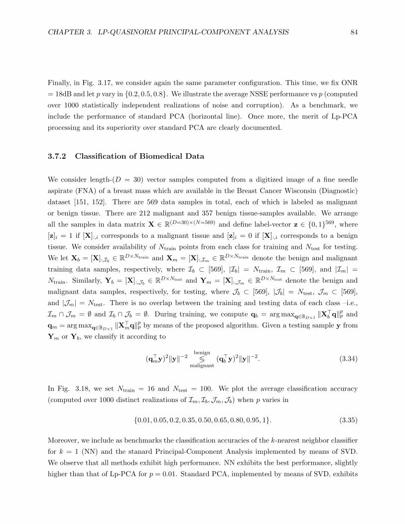
CHAPTER 3. LP-QUASINORM PRINCIPAL-COMPONENT ANALYSIS 84
Finally, in Fig. 3.17, we consider again the same parameter configuration. This time, we fix ONR
= 18dB and let p vary in 0.2, 0.5, 0.8. We illustrate the average NSSE performance vs p (computed
over 1000 statistically independent realizations of noise and corruption). As a benchmark, we
include the performance of standard PCA (horizontal line). Once more, the merit of Lp-PCA
processing and its superiority over standard PCA are clearly documented.
3.7.2 Classification of Biomedical Data
We consider length-(D = 30) vector samples computed from a digitized image of a fine needle
aspirate (FNA) of a breast mass which are available in the Breast Cancer Wisconsin (Diagnostic)
dataset [151, 152]. There are 569 data samples in total, each of which is labeled as malignant
or benign tissue. There are 212 malignant and 357 benign tissue-samples available. We arrange
all the samples in data matrix X ∈ R(D=30)×(N=569) and define label-vector z ∈ 0, 1569, where
[z]i = 1 if [X]:,i corresponds to a malignant tissue and [z]i = 0 if [X]:,i corresponds to a benign
tissue. We consider availability of Ntrain points from each class for training and Ntest for testing.
We let Xb = [X]:,Ib ∈ RD×Ntrain and Xm = [X]:,Im ∈ RD×Ntrain denote the benign and malignant
training data samples, respectively, where Ib ⊂ [569], |Ib| = Ntrain, Im ⊂ [569], and |Im| =
Ntrain. Similarly, Yb = [X]:,Jb ∈ RD×Ntest and Ym = [X]:,Jm ∈ RD×Ntest denote the benign and
malignant data samples, respectively, for testing, where Jb ⊂ [569], |Jb| = Ntest, Jm ⊂ [569],
and |Jm| = Ntest. There is no overlap between the training and testing data of each class –i.e.,
Im ∩ Jm = ∅ and Ib ∩ Jb = ∅. During training, we compute qb = arg maxq∈BD×1‖X>b q‖pp and
qm = arg maxq∈BD×1‖X>mq‖pp by means of the proposed algorithm. Given a testing sample y from
Ym or Yb, we classify it according to
(q>my)2‖y‖−2benign
≶malignant
(q>b y)2‖y‖−2. (3.34)
In Fig. 3.18, we set Ntrain = 16 and Ntest = 100. We plot the average classification accuracy
(computed over 1000 distinct realizations of Im, Ib,Jm,Jb) when p varies in
0.01, 0.05, 0.2, 0.35, 0.50, 0.65, 0.80, 0.95, 1. (3.35)
Moreover, we include as benchmarks the classification accuracies of the k-nearest neighbor classifier
for k = 1 (NN) and the stanard Principal-Component Analysis implemented by means of SVD.
We observe that all methods exhibit high performance. NN exhibits the best performance, slightly
higher than that of Lp-PCA for p = 0.01. Standard PCA, implemented by means of SVD, exhibits

CHAPTER 3. LP-QUASINORM PRINCIPAL-COMPONENT ANALYSIS 85
0 0.2 0.4 0.6 0.8 1p
0.7
0.75
0.8
0.85
0.9
Acc
urac
y
Lp-PCA (proposed)PCA benchmarkNearest neighbor benchmark
Figure 3.18. Breast Cancer Wisconsin (Diagnostic) Dataset: Classification accuracy vs p. Ntrain =20, Ntest = 100, m = 0.
0 0.2 0.4 0.6 0.8 1p
0.7
0.75
0.8
0.85
0.9
Acc
urac
y
Lp-PCA (proposed)PCA benchmarkNearest neighbor benchmark
Figure 3.19. Breast Cancer Wisconsin (Diagnostic) Dataset: Classification accuracy vs p. Ntrain =20, Ntest = 100, m = 3.
the lowest performance.
In Fig. 3.19, we repeat the above experiment but this time we consider that m = 3 malignant
samples have mistakenly been labeled as benign samples and m = 3 benign samples have been
mislabeled as malignant. We notice that the performances of NN and SVD are significantly com-
promised by the mislabelings –i.e., the performance of NN dropped to 0.74 from 0.89 and the
performance of PCA dropped to 0.71 from 0.85. On the other hand, Lp-PCA attained classifica-
tion performance as high as 0.88 (p = 0.1) and no lower than 0.825 (p = 1).
Finally, in Fig. 3.20, we set Ntrain = 20, Ntest = 100, and p = 0.1. We let the number of
mislabelings, m, vary in 0, 1, 2, 3, 4.2 Then, we plot the classification accuracy attained by each
method (computed over 1000 distinct realizations of data and corruptions). Expectedly, when
m = 0 the performances of all methods are similar to their performances in Fig. 3.18. However, as
2That is, m benign samples have wrongly been labeled as malignant and m malignant samples have been labeledas benign samples.
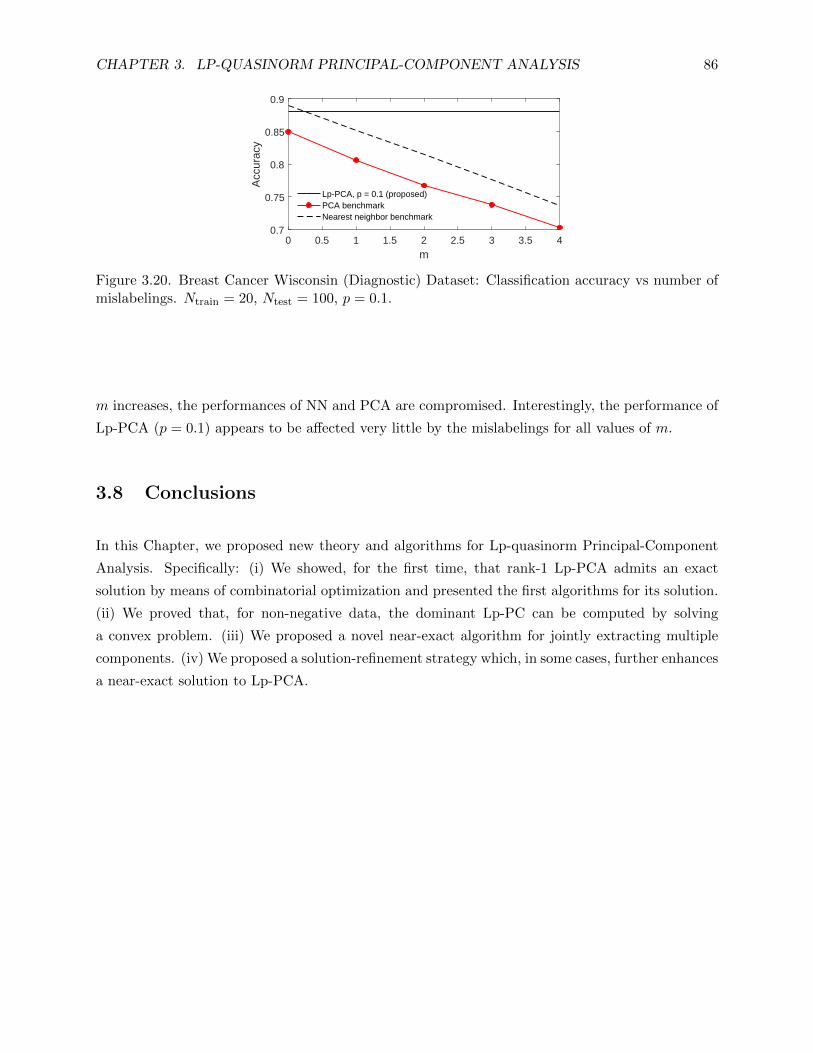
CHAPTER 3. LP-QUASINORM PRINCIPAL-COMPONENT ANALYSIS 86
0 0.5 1 1.5 2 2.5 3 3.5 4m
0.7
0.75
0.8
0.85
0.9
Acc
urac
y
Lp-PCA, p = 0.1 (proposed)PCA benchmarkNearest neighbor benchmark
Figure 3.20. Breast Cancer Wisconsin (Diagnostic) Dataset: Classification accuracy vs number ofmislabelings. Ntrain = 20, Ntest = 100, p = 0.1.
m increases, the performances of NN and PCA are compromised. Interestingly, the performance of
Lp-PCA (p = 0.1) appears to be affected very little by the mislabelings for all values of m.
3.8 Conclusions
In this Chapter, we proposed new theory and algorithms for Lp-quasinorm Principal-Component
Analysis. Specifically: (i) We showed, for the first time, that rank-1 Lp-PCA admits an exact
solution by means of combinatorial optimization and presented the first algorithms for its solution.
(ii) We proved that, for non-negative data, the dominant Lp-PC can be computed by solving
a convex problem. (iii) We proposed a novel near-exact algorithm for jointly extracting multiple
components. (iv) We proposed a solution-refinement strategy which, in some cases, further enhances
a near-exact solution to Lp-PCA.
Chapter 4
Coprime Array Processing
4.1 Introduction
Coprime Arrays (CAs) are non-uniform linear arrays the element locations of which are derived by
coprime number theory [153]. CAs are a special class of sparse arrays [153, 154] which are often
preferred due to their desirable bearing properties –i.e., enhanced Degrees-of-Freedom (DoF) and
closed-form expressions for element-locations. CAs have attracted significant research interest over
the past years and have been successfully employed in applications such as Direction-of-Arrival
(DoA) estimation [155–166], beamforming [167–169], interference localization and mitigation in
satellite systems [170], and space-time adaptive processing [171, 172], to name a few.
Interpolation methods for CAs which further enhance DoF [173–180] have also been studied. Fur-
thermore, scholars have considered CAs for underwater localization [181, 182], channel estimation
in MIMO communications via tensor decomposition [183], receivers capable of two-dimensional
DoA estimation [184], and receivers on moving platforms which also promote increased number of
DoF [185–187]. Other non-uniform arrays with increased DoF and closed-form expressions are the
nested and MISC arrays [154, 188].
In standard DoA estimation with CAs [153], the receiver conducts a series of intelligent process-
ing steps and assembles an autocorrelation matrix which corresponds to a larger virtual Uniform
Linear Array (ULA) which is commonly referred to as coarray. Accordingly, CAs enable the iden-
tification of more sources than sensors compared to equal-length ULAs [189–195]. Processing at a
coprime array receiver commences with the estimation of the nominal (true) physical-array auto-
87

CHAPTER 4. COPRIME ARRAY PROCESSING 88
correlations. The receiver processes the estimated autocorrelations so that each coarray element is
represented by one autocorrelation estimate. Next, the processed autocorrelations undergo spatial
smoothing, forming an autocorrelation matrix estimate which corresponds to the coarray. By the
received-signal model, the nominal autocorrelation matrix of the coarray has a specific structure:
it is (i) Positive Definite (PD), (ii) Hermitian, (iii) Toeplitz, and (iv) its noise-subspace eigenvalues
are equal. Finally, a DoA estimation approach such as the MUltiple SIgnal Classification (MU-
SIC) algorithm, for instance, can be applied to the resulting autocorrelation matrix estimate for
identifying the source directions.
In practice, the autocorrelations of the physical-array elements are estimated by processing a col-
lection of received-signal snapshots and diverge from the nominal ones. Accordingly, existing ap-
proaches offer autocorrelation-matrix estimates which diverge from the nominal one, while at the
same time, violate at least one of the above structure-properties. At the autocorrelation pro-
cessing step, the estimated autocorrelations are commonly processed by selection combining [153],
retaining only one autocorrelation sample for each coarray element. Alternatively, an autocor-
relation estimate for each coarray element is obtained by averaging combining [162] all available
sample-estimates corresponding to a particular coarray element. The two methods coincide in
Mean-Squared-Error (MSE) estimation performance when applied to the nominal physical-array
autocorrelations –which the receiver could only estimate with asymptotically large number of
received-signal snapshots. Due to a finite number of received-signal snapshots available at the
receiver and the fact that these methods have been designed under no optimality criterion, the
estimated autocorrelations diverge from the nominal ones and attain arbitrary MSE performance.
In this case, the two methods no longer coincide in MSE estimation performance.
In this Chapter, we focus on the autocorrelation combining step of coprime array processing and
make the following contributions:
Contribution i. For the first time, we present in closed-form the MSE of both selection and averag-
ing autocorrelation combining and show that, for any number of sample support,
averaging combining offers superior MSE estimation performance compared to
selection combining. The theoretical results are validated with numerical simu-
lations.
Contribution ii. Motivated by prior works which treat source angles as statistical random vari-
ables [196, 197], we make the mild assumption that the source directions are inde-
pendently and identically distributed random variables. Under this assumption,
we design a novel coprime array receiver equipped with a linear autocorrelation

CHAPTER 4. COPRIME ARRAY PROCESSING 89
combiner designed under the Minimum-MSE (MMSE) optimality criterion. The
proposed MMSE combiner minimizes in the mean –i.e., for any configuration of
DoAs– the error in estimating the physical-array autocorrelations with respect to
the MSE metric. We conduct extensive numerical studies and compare the per-
formance of the proposed MMSE combiner to existing counterparts, with respect
to autocorrelation estimation error and DoA estimation.
Contribution iii. We propose an optimization framework for computing an improved coarray au-
tocorrelation matrix estimate that satisfies the structure properties (i)-(iv). In
practice, we iteratively solve a sequence of distinct structure-optimization prob-
lems, obtaining upon convergence, an improved estimate that satisfies properties
(i)-(iv). The proposed framework is accompanied by formal convergence analy-
sis. Numerical studies illustrate that the proposed method outperforms standard
counterparts, both in estimation error and DoA estimation.
The rest of this Chapter is organized as follows. In Section 4.2, we present the signal model and state
the problem of interest. In Section 4.3, we review the existing selection and averaging autocorrela-
tion combining methods for coprime arrays and existing coarray autocorrelation matrix estimates.
In Section 4.4, we present the closed-form expressions of selection and averaging autocorrelation
combining approaches. Then, in Section 4.5, we present the proposed MMSE autocorrelation com-
bining. After, in Section 4.6, we present the proposed structured coarray autocorrelation matrix
estimate. Conclusions are drawn in Section 4.7.
The contributions presented in this Chapter have also been presented in [155, 156, 198, 199].
4.2 Signal Model and Problem Statement
Consider coprime naturals (M,N) such that M < N . A coprime array equipped with L = 2M+N−1 elements is formed by overlapping a ULA with N antenna elements at positions pM,i = (i−1)M∆,
i = 1, 2, . . . , N , and a ULA equipped with 2M − 1 antenna elements at positions pN,i = iN∆,
i = 1, 2, . . . , 2M − 1. The reference unit-spacing ∆ is typically set to one-half wavelength at the
operating frequency. The positions of the L elements are the entries of the element-location vector
p4= sort([pM,1, . . . , pM,N , pN,1, . . . , pN,2M−1]>), where sort(·) sorts the entries of its vector argument
in ascending order and the superscript ‘>’ denotes matrix transpose. We assume that narrowband
signals impinge on the array from K < MN + M sources with propagation speed c and carrier

CHAPTER 4. COPRIME ARRAY PROCESSING 90
frequency fc. Assuming far-field conditions, a signal from source k ∈ 1, 2, . . . ,K impinges on
the array from direction θk ∈ (−π2 ,
π2 ] with respect to the broadside. The array response vector
for source k is s(θk)4= [v(θk)
[p]1 , . . . , v(θk)[p]L ]> ∈ CL×1, with v(θ)
4= exp
(−j2πfc
c sin(θ))
for every
θ ∈ (−π2 ,
π2 ]. Accordingly, the qth collected received-signal snapshot is of the form
yq =K∑k=1
s(θk)ξq,k + nq ∈ CL×1, (4.1)
where ξq,k ∼ CN (0, dk) is the qth symbol for source k (power-scaled and flat-fading-channel pro-
cessed) and nq ∼ CN (0L, σ2IL) models Additive White Gaussian Noise (AWGN). We make the
common assumptions that the random variables are statistically independent across different snap-
shots and that symbols from different sources are independent of each other and of every entry of
nq. The received-signal autocorrelation matrix is given by
Ry4= EyqyHq = S diag(d) SH + σ2IL, (4.2)
where d4= [d1, . . . , dK ]> ∈ RK×1
+ is the source-power vector and S4= [s(θ1), . . . , s(θK)] ∈ CL×K is
the array-response matrix. We define
r4= vec(Ry) =
K∑i=1
a(θi)di + σ2iL ∈ CL2×1, (4.3)
where vec(·) returns the column-wise vectorization of its matrix argument, a(θi)4= s(θi)
∗ ⊗ s(θi),
iL4= vec(IL), the superscript ‘∗’ denotes complex conjugate, and ‘⊗’ is the Kronecker product of
matrices [200]. By coprime number theory [153], for every n ∈ −L′ + 1,−L′ + 2, . . . , L′ − 1 with
L′4= MN +M , there exists a well-defined set of indices Jn ⊂ 1, 2, . . . , L2, such that
[a(θ)]j = v(θ)n ∀j ∈ Jn, (4.4)
for every θ ∈ (−π2 ,
π2 ]. We henceforth consider that Jn contains all j indices that satisfy (4.4). In
view of (4.4), a coprime array receiver assembles a linear combining matrix E ∈ RL2×(2L′−1) and
forms a length-(2L′ − 1) autocorrelation-vector rco, each element of which corresponds to a single
set Jn, for every n ∈ 1 − L′, 2 − L′, . . . , L′ − 1, by conducting linear processing1 (e.g., E>r) to
1Existing coprime array autocorrelation processing methods in the literature are reviewed in Section 4.3.

CHAPTER 4. COPRIME ARRAY PROCESSING 91
the autocorrelations in r. That is, there exists linear combiner E such that
rco = E>r =
K∑k=1
aco(θk)dk + σ2eL′,2L′−1, (4.5)
where aco(θ)4= [v(θ)1−L′ , v(θ)2−L′ , . . . , v(θ)L
′−1] for any θ ∈ (−π2 ,
π2 ], and, for any p ≤ P ∈ N+,
ep,P is the pth column of IP . Thereafter, the receiver applies spatial-smoothing to organize the
sampled autocorrelations as the matrix
Z4= Φ (rco)
4= F(IL′ ⊗ rco) ∈ CL
′×L′ , (4.6)
where F4= [F1,F2, . . . ,FL′ ] and Fm
4= [0L′×(L′−m), IL′ ,0L′×(m−1)] ∀m ∈ 1, 2, . . . , L′. This ap-
proach is also known as the Augmented Matrix in the coprime array processing literature [162].
Importantly, under nominal statistics Z becomes the autocorrelation matrix of a length-L′ ULA
with antenna elements at locations 0, 1, . . . , L′ − 1∆. That is,
Z = Scodiag(d)SHco + σ2IL′ , (4.7)
where it holds that [Sco]m,k = v(θk)m−1 for everym ∈ 1, 2, . . . , L′ and k ∈ 1, 2, . . . ,K. Standard
MUSIC DoA estimation can be applied to Z. Let the columns of U ∈ CL′×K be the dominant
left-hand singular vectors of Z, corresponding to its K highest singular values, acquired by means
of Singular Value Decomposition (SVD). Defining v(θ) = [1, v(θ), . . . , v(θ)L′−1]>, we can accurately
decide that θ ∈ (−π2 ,
π2 ] belongs in Θ
4= θ1, θ2, . . . , θK if (IL′ −UUH)v(θ) = 0L′ is satisfied for
some θ. Equivalently, we can resolve the angles in Θ by the K (smallest) local minima of the
standard MUSIC spectrum [201]
PMUSIC(θ) =∥∥(IL′ −UUH
)v(θ)
∥∥2
2. (4.8)
In practice, Ry in (4.2) is unknown to the receiver and sample-average estimated by a collection of
Q received-signal snapshots in Y = [y1,y2, . . . ,yQ] by
Ry =1
Q
Q∑q=1
yqyHq . (4.9)

CHAPTER 4. COPRIME ARRAY PROCESSING 92
Snapshot
Autocorrelation
Autocorrelation
CombiningSmoothing SVD
Figure 4.1. Coprime processing steps: from a collection of samples yqQq=1 to the estimated coarraysignal-subspace basis U.
Accordingly, the physical-array autocorrelation-vector r in (4.3) is estimated by
r4= vec(Ry) =
1
Q
Q∑q=1
y∗q ⊗ yq. (4.10)
The receiver then conducts linear combining to the estimated autocorrelation vector r to obtain an
estimate of rco, rco = E>r. The estimation error ‖rco − rco‖2 depends on how well the linear com-
biner E estimates the nominal physical-array autocorrelations. Accordingly, Z in (4.7) is estimated
by Z4= Φ (rco).
Finally, MUSIC DoA estimation can be applied using the K dominant left-hand singular vectors
of Z instead of those of Z. Of course, in practice, there is an inherent DoA estimation error due
to the mismatch between Z and Z. A schematic illustration of the coprime array processing steps
presented above is offered in Fig. 4.1.
4.3 Technical Background
4.3.1 Selection Combining
The most commonly considered autocorrelation combining method is selection combining [153]
based on which the receiver selects any single index jn ∈ Jn, for n ∈ −L′ + 1, . . . , L′ − 1,and forms the selection combining matrix
Esel4=[ej1−L′ ,L2 , ej2−L′ ,L2 , . . . , ejL′−1,L
2
]∈ RL
2×(2L′−1), (4.11)
CHAPTER 4. COPRIME ARRAY PROCESSING 93
by which it processes the autocorrelations in r, discarding by selection all duplicates –i.e., every
entry with index in Jn \ jn, for every n– to form autocorrelation vector
rsel4= E>selr ∈ R2L′−1. (4.12)
Importantly, when the nominal entries of r are known to the receiver, rsel coincides with rco in (4.5),
thus, applying spatial smoothing on rsel yields the exact coarray autocorrelation matrix Z = Φ (rsel).
In contrast, when r is unknown to the receiver and estimated by r in (4.10), rsel in (4.12) is estimated
by
rsel = E>selr ∈ R2L′−1. (4.13)
Accordingly, the coarray autocorrelation matrix is estimated by Zsel4= Φ (rsel).
4.3.2 Averaging Combining
Instead of selecting a single index in Jn by discarding duplicates, averaging combining [162] conducts
averaging on all autocorrelation estimates in Jn, for every n ∈ 1−L′, 2−L′, . . . , L′− 1. That is,
the receiver forms the averaging combining matrix
Eavg4=
1
|J1−L′ |∑
j∈J1−L′
ej,L2 , . . . ,1
|JL′−1|∑
j∈JL′−1
ej,L2
. (4.14)
| · | denotes the cardinality (number of elements in a set) of its argument. Then, it processes the
autocorrelation vector r to obtain
ravg4= E>avgr ∈ R2L′−1. (4.15)
By (4.4) and the fact that [iL]j equals 1, if j ∈ J0 and 0 otherwise, it holds that, for any n ∈−L′ + 1, . . . , L′ − 1, [r]j = e>j,L2r takes a constant value for every j ∈ Jn. Thus, ravg coincides
with rsel and rco. Therefore, similar to the selection combining approach, when r is known to the
receiver, applying spatial smoothing on ravg yields Z = Φ (ravg). In practice, when Ry in (4.2) is
estimated by Ry in (4.9), ravg is estimated by
ravg4= Eavg
>r ∈ R2L′−1. (4.16)
CHAPTER 4. COPRIME ARRAY PROCESSING 94
Accordingly, Z is estimated by Zavg4= Φ (ravg).
4.3.3 Remarks on Existing Coarray Autocorrelation Matrix Estimates
The true coarray autocorrelation matrix Z has full-rank, is PD, Hermitian, and Toeplitz. If we
consider Zss4= 1
L′ZZH , then an autocorrelation matrix estimate can be extracted from Zss as a
scaled version of its Principal Squared Root (PSR) [153]
Zpsr4=√L′Z
12ss. (4.17)
We notice that ZZH = Z2 = L′Zss. Moreover, Zss admits SVD Zsssvd= UΛVH which implies that
Zpsr = U(√L′Λ
12 )VH = Z. That is, Zpsr and Z coincide. Accordingly, in the (ideal) case of known
statistics to the receiver, all estimates that we have discussed above coincide with the nominal
autocorrelation matrix of the coarray and satisfy (i)-(iv).
However, in the practical case of unknown statistics (case of interest) to the receiver, the estimates
above diverge from Z and satisfy only a subset of (i)-(iv): That is, Zavg and Zsel are guaranteed
to be Hermitian and Toeplitz, however, they are not guaranteed to be PD –i.e., Zavg and Zsel can
be indefinite estimates of Z [162]. Similarly, by adopting the superior averaging autocorrelation
combining approach, Zss and Zpsr can be estimated by Zss4= 1
L′ ZavgZHavg and Zpsr
4=√L′Z
12ss,
respectively. In view of the above, Zpsr is by construction a PD and Hermitian matrix estimate
of the coarray autocorrelation matrix, however, it violates the Toeplitz structure-property of Z.
It follows that Zpsr and Zavg no longer coincide, however, their left-hand singular-valued singular
vectors span the same signal subspace.
4.4 Contribution 1: Closed-form MSE Expressions for Selection
and Averaging Combining
In general, estimates rsel and ravg diverge from rco and attain MSE errr(rsel)4= E‖rco − rsel‖22
and errr(ravg), respectively. Zsel and Zavg diverge from the true Z and attain MSE errZ(Zsel)4=
E‖Z − Zsel‖2F and errZ(Zavg), respectively. In this Section, we present for the first time closed-
form MSE expressions for the estimation errors attained by selection and averaging combining.
For any sample support Q, the following Lemma 4.1 and Lemma 4.2 express in closed-form the

CHAPTER 4. COPRIME ARRAY PROCESSING 95
MSE attained by rsel.
Lemma 4.1. For any n ∈ −L′ + 1,−L′ + 2, . . . , L′ − 1 and j ∈ Jn, it holds
e = E|[r]j − [r]j |2 =(1>Kd + σ2)2
Q. (4.18)
Lemma 4.2. rsel attains MSE errr(rsel) = (2L′ − 1) e.
In view of Lemma 4.2, the following Proposition naturally follows.
Proposition 4.1. Zsel attains MSE errZ(Zsel) = L′2e.
Expectedly, as the sample-support Q grows asymptotically, e, errr(rsel), and errZ(Zsel) converge to
zero.
For any sample support Q, the following Lemma 4.3 and Lemma 4.4 express in closed-form the MSE
attained by ravg, where p4= p⊗ 1L, ωi,j
4= [p]i− [p]j , and zi,j
4= [v(θ1)ωi,j v(θ2)ωi,j . . . v(θK)ωi,j ]H .
Lemma 4.3. For any n ∈ −L′ + 1, . . . , L′ − 1 and jn ∈ Jn, it holds that
en = E
∣∣∣∣∣∣[r]jn −
1
|Jn|∑j∈Jn
[r]j
∣∣∣∣∣∣2 =
1
Q
2σ21>Kd + σ4
|Jn|+∑i∈Jn
∑j∈Jn
|zHi,jd|2
|Jn|2
. (4.19)
Lemma 4.4. ravg attains MSE errr(ravg) =∑L′−1
n=1−L′ en.
By Lemma 4.4, the following Proposition naturally follows.
Proposition 4.2. Zavg attains MSE errZ(Zavg) =L′∑m=1
L′−m∑n=1−m
en.
Similar to selection combining, as the sample-support Q grows asymptotically, en, errr(ravg), and
errZ(Zavg) converge to zero. Complete proofs for the above Lemmas and Propositions are offered
for the first time in the Appendix.

CHAPTER 4. COPRIME ARRAY PROCESSING 96
Remarks on Selection and Averaging Combining
In view of (4.19), e = en, when |Jn| = 1. Also, (4.18) and (4.19) show that, as expected, e and en
tend to zero as Q increases asymptotically. Using (4.18) and (4.19), we prove below the inequality
en ≤ e, which documents the MSE superiority of average-sampling over selection-sampling. We
observe that, for any i, j, |zHi,jd|2 = |∑K
k=1[zi,j ]∗kdk|2 ≤ |
∑Kk=1 |[zi,j ]∗kdk||2 = (1>Kd)2 and, therefore,
e− en ≥ βn4=|Jn| − 1
|Jn|Q(2σ21>Kd + σ4) ≥ 0. (4.20)
4.4.1 Numerical Studies
We consider an (M = 2, N = 3) extended coprime array of L = 6 elements and K = 7 sources,
transmitting from angles Θ = θ1 = −60, θ2 = −28, θ3 = −4, θ4 = 5, θ5 = 18, θ6 = 34, θ7 =
86. We set σ2 = 1 and signal-to-noise ratio (SNR) to 10dB, for all K sources; i.e., dk = 10 ∀k.
First, we let the number of snapshots Q vary from 20 to 140 in increments of 10. For each value of Q,
we simulate estimation of Z by both selection-sampling (Zsel) and averaging-sampling (Zavg); then,
we measure the corresponding squared-estimation errors ‖Z− Zsel‖2F and ‖Z− Zavg‖2F . We repeat
this procedure for 10, 000 independent symbol/noise realizations and plot the averaged squared-
error in Fig. 4.2. In the same figure, we plot the theoretical MSEs errZ(Zsel) and errZ(Zavg), as
presented in Proposition 4.1 and Proposition 4.2, respectively. We observe that the numerically
and theoretically calculated values for the MSEs coincide. All MSE curves start from a high value
for Q = 20 and decrease monotonically as Q increases, with a trend for asymptotic convergence to
0, as Q → ∞. We observe that, in accordance to Proposition 4.1 and Proposition 4.2, errZ(Zavg)
is significantly lower than errZ(Zsel), for every value of Q.
Next, we set Q = 30 and calculate the MSE of selection and averaging in the estimation of Z for
different values of K. Specifically, in Fig. 4.3, we plot the theoretical and numerical MSEs attained
by the two estimators versus the number of transmitting sources, K = 1, 2, . . . , 7, i.e., for K = 1,
we consider signal transmission only from angle θ1 = −60 in Θ, while for K = 3, we consider
transmission from angles θ1 = −60, θ2 = −28, and θ3 = −4. We observe that the performance
gap between selection and averaging increases monotonically with K. This is in accordance with the
observation that the lower-bound of the gap, βn in (4.20), increases monotonically as K increases,
for every n such that |Jn| > 1 (when |Jn| = 1, βn = 0).
In the next two examples, we examine the association between the MSE in the estimation of Z
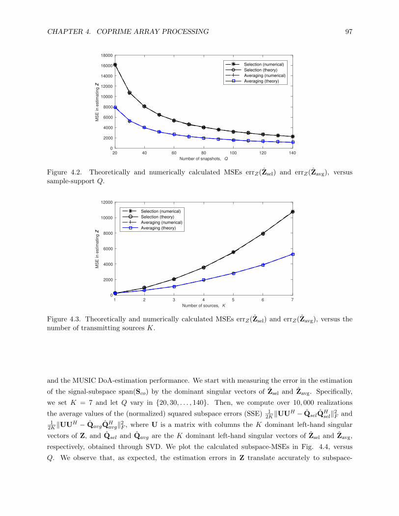
CHAPTER 4. COPRIME ARRAY PROCESSING 97
20 40 60 80 100 120 140
Number of snapshots, Q
0
2000
4000
6000
8000
10000
12000
14000
16000
18000
MS
E in
estim
atin
g Z
Selection (numerical)
Selection (theory)
Averaging (numerical)
Averaging (theory)
Figure 4.2. Theoretically and numerically calculated MSEs errZ(Zsel) and errZ(Zavg), versussample-support Q.
1 2 3 4 5 6 7
Number of sources, K
0
2000
4000
6000
8000
10000
12000
MS
E in
estim
atin
g Z
Selection (numerical)
Selection (theory)
Averaging (numerical)
Averaging (theory)
Figure 4.3. Theoretically and numerically calculated MSEs errZ(Zsel) and errZ(Zavg), versus thenumber of transmitting sources K.
and the MUSIC DoA-estimation performance. We start with measuring the error in the estimation
of the signal-subspace span(Sco) by the dominant singular vectors of Zsel and Zavg. Specifically,
we set K = 7 and let Q vary in 20, 30, . . . , 140. Then, we compute over 10, 000 realizations
the average values of the (normalized) squared subspace errors (SSE) 12K ‖UUH − QselQ
Hsel‖2F and
12K ‖UUH − QavgQ
Havg‖2F , where U is a matrix with columns the K dominant left-hand singular
vectors of Z, and Qsel and Qavg are the K dominant left-hand singular vectors of Zsel and Zavg,
respectively, obtained through SVD. We plot the calculated subspace-MSEs in Fig. 4.4, versus
Q. We observe that, as expected, the estimation errors in Z translate accurately to subspace-

CHAPTER 4. COPRIME ARRAY PROCESSING 98
20 40 60 80 100 120 140
Number of snapshots, Q
0
0.02
0.04
0.06
0.08
0.1
Ave
rag
e S
SE
Selection
Averaging
Figure 4.4. Average squared subspace error attained by selection and averaging sampling, versussample-support Q.
20 40 60 80 100 120 140
Number of snapshots, Q
3
4
5
6
7
8
9
10
11
12
RM
SE
(in
de
g)
Selection
Averaging
Figure 4.5. RMSE of coprime MUSIC DoA estimation attained by selection and averaging sampling,versus sample-support Q.
estimation errors. Thus, averaging autocorrelation sampling attains lower subspace estimation
error than selection sampling, for every value of Q, with the maximum difference documented at
the minimum tested value of Q.
Finally, for the same setup (K = 7, Q = 20, 30, . . . , 140), we conduct MUSIC DoA estimation in the
form of (4.8), employing, instead of the ideal signal-subspace descriptor UUH , the estimated projec-
tion matrices QselQHsel (selection) and QavgQ
Havg (sampling), calculated upon the estimates Zsel and
Zavg, respectively. After 10, 000 independent realizations, we compute and plot in Fig. 4.5 the root-
mean-squared-error (RMSE) for the two estimators, RMSE =√
1K
∑Kk=1
110000
∑10000r=1 (θk − θk,r)2,
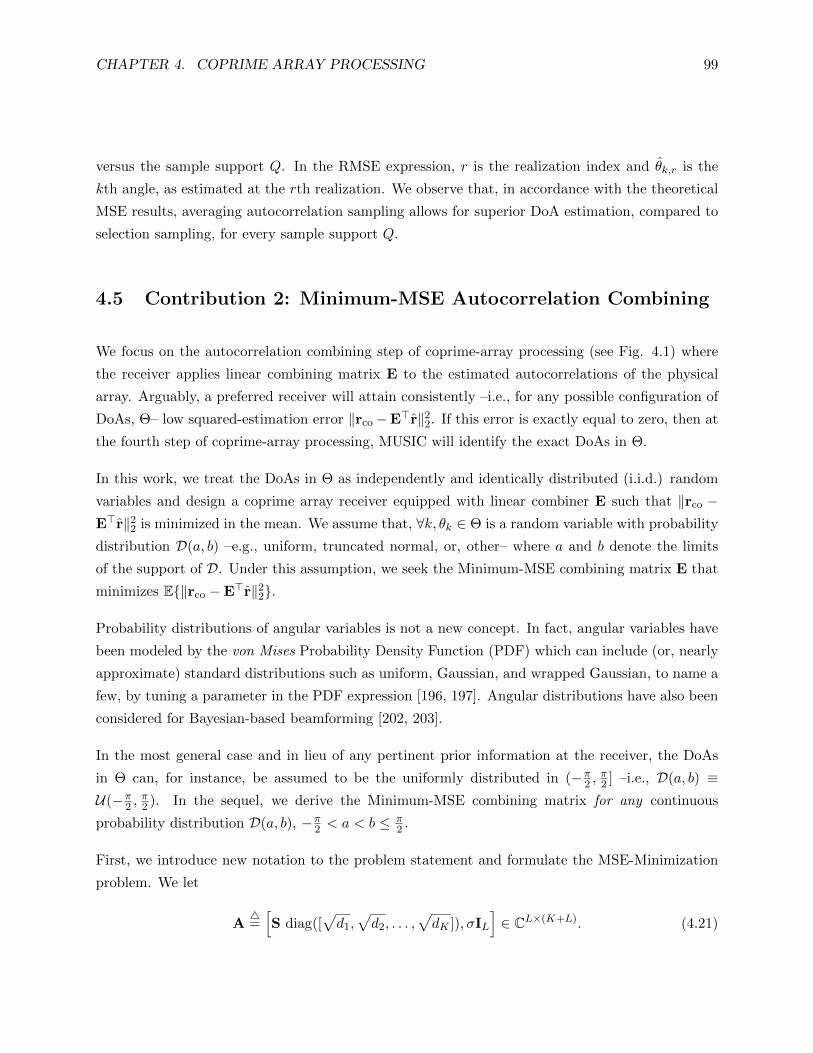
CHAPTER 4. COPRIME ARRAY PROCESSING 99
versus the sample support Q. In the RMSE expression, r is the realization index and θk,r is the
kth angle, as estimated at the rth realization. We observe that, in accordance with the theoretical
MSE results, averaging autocorrelation sampling allows for superior DoA estimation, compared to
selection sampling, for every sample support Q.
4.5 Contribution 2: Minimum-MSE Autocorrelation Combining
We focus on the autocorrelation combining step of coprime-array processing (see Fig. 4.1) where
the receiver applies linear combining matrix E to the estimated autocorrelations of the physical
array. Arguably, a preferred receiver will attain consistently –i.e., for any possible configuration of
DoAs, Θ– low squared-estimation error ‖rco−E>r‖22. If this error is exactly equal to zero, then at
the fourth step of coprime-array processing, MUSIC will identify the exact DoAs in Θ.
In this work, we treat the DoAs in Θ as independently and identically distributed (i.i.d.) random
variables and design a coprime array receiver equipped with linear combiner E such that ‖rco −E>r‖22 is minimized in the mean. We assume that, ∀k, θk ∈ Θ is a random variable with probability
distribution D(a, b) –e.g., uniform, truncated normal, or, other– where a and b denote the limits
of the support of D. Under this assumption, we seek the Minimum-MSE combining matrix E that
minimizes E‖rco −E>r‖22.
Probability distributions of angular variables is not a new concept. In fact, angular variables have
been modeled by the von Mises Probability Density Function (PDF) which can include (or, nearly
approximate) standard distributions such as uniform, Gaussian, and wrapped Gaussian, to name a
few, by tuning a parameter in the PDF expression [196, 197]. Angular distributions have also been
considered for Bayesian-based beamforming [202, 203].
In the most general case and in lieu of any pertinent prior information at the receiver, the DoAs
in Θ can, for instance, be assumed to be the uniformly distributed in (−π2 ,
π2 ] –i.e., D(a, b) ≡
U(−π2 ,
π2 ). In the sequel, we derive the Minimum-MSE combining matrix for any continuous
probability distribution D(a, b), −π2 < a < b ≤ π
2 .
First, we introduce new notation to the problem statement and formulate the MSE-Minimization
problem. We let
A4=[S diag([
√d1,√d2, . . . ,
√dK ]), σIL
]∈ CL×(K+L). (4.21)

CHAPTER 4. COPRIME ARRAY PROCESSING 100
The autocorrelation matrix Ry in (4.2) is factorized as Ry = AAH . Then, we define
V4= A∗ ⊗A ∈ CL
2×(K+L)2 (4.22)
and i4= vec(IK+L) ∈ R(K+L)2 , where IK+L is the (K + L)-size identity matrix. It follows that r
takes the form
r = Vi. (4.23)
In view of the above, rco (or, rsel and ravg in (4.12) and (4.15), respectively) can be expressed as
E>selVi = E>avgVi. We observe that ∀q ∈ 1, 2, . . . , Q, there exists vector xq ∼ CN (0K+L, IK+L),
pertinent to yq, such that yq = Axq. By the signal model, xq is statistically independent from xp
for any (p, q) ∈ 1, 2, . . . , Q2 such that p 6= q. The physical-array autocorrelation matrix estimate
Ry in (4.9) is expressed as Ry = AWAH , where W4= 1
Q
∑Qq=1 xqx
Hq . Moreover, by defining
w4= vec (W) = 1
Q
∑Qq=1 x∗q ⊗ xq, the estimate r in (4.10) takes the form
r = Vw. (4.24)
By (4.23) and (4.24), we propose to design linear combiner EMMSE by formulating and solving the
MSE-Minimization
arg minE∈CL2×(2L′−1)
EΘ,w
∥∥∥EHVw −E>selVi∥∥∥2
2
. (4.25)
Of course, if we replace Esel by Eavg in (4.25), the resulting problem will be equivalent. In the
sequel, we show that a closed-form solution to (4.25) exists for any finite value of sample support
Q and present it step-by-step.
We commence our solution by defining G4= VwwHVH ∈ CL2×L2
and H4= VwiHVH ∈ CL2×L2
.
Then, the problem in (4.25) simplifies to
arg minE∈CL2×(2L′−1)
EΘ,w
Tr(EHGE
)− 2<
Tr(EHHEsel
), (4.26)
where <· extracts the real part of its argument and Tr(·) returns the sum of the diagonal entries
of its argument. Furthermore, we define GE4= EΘ,wG and HE
4= EΘ,wH. Then, (4.26) takes

CHAPTER 4. COPRIME ARRAY PROCESSING 101
PD
F
Figure 4.6. Probability density function f(θ) for different distributions and support sets.
the equivalent form
arg minE∈CL2×(2L′−1)
Tr(EHGEE
)− 2<
Tr(EHHEEsel
). (4.27)
Next, we focus on deriving closed-form expressions for GE and HE that will allow us to solve (4.27)
and obtain the Minimum-MSE linear combiner EMMSE. At the core of our developments lies the
observation that, ∀θ ∼ D(a, b) with PDF f(θ) and scalar x ∈ R, it holds
I(x)4= E
θv(θ)x =
∫ b
af(θ)exp
(−jx2πfc
csin θ
)dθ. (4.28)
The integral I(x) can be approximated within some numerical error tolerance with numerically
efficient vectorized methods [204–206]. In Fig. 4.6, we offer visual illustration examples of f(θ)
when θ follows a uniform distribution in (a, b) –i.e., θ ∼ U(a, b)– or, a truncated normal distribution
in (a, b) with mean µ and variance σ2 –i.e., θ ∼ T N (a, b, µ, σ2).
That is,
f(θ) =
1
σ√2π
exp(− 1
2( θ−µσ )2)
12
(erf(b−µσ√
2
)−erf
(a−µσ√2
)) , θ ∼ T N (a, b, µ, σ2),
1b−a , θ ∼ U(a, b),
(4.29)
where erf(·) denotes the Error Function [207]. In the special case that D(a, b) ≡ U(−π2 ,
π2 ), I(x)
coincides with J0(x2πfcc ): the 0th order Bessel function of the first kind [208] for which there exist
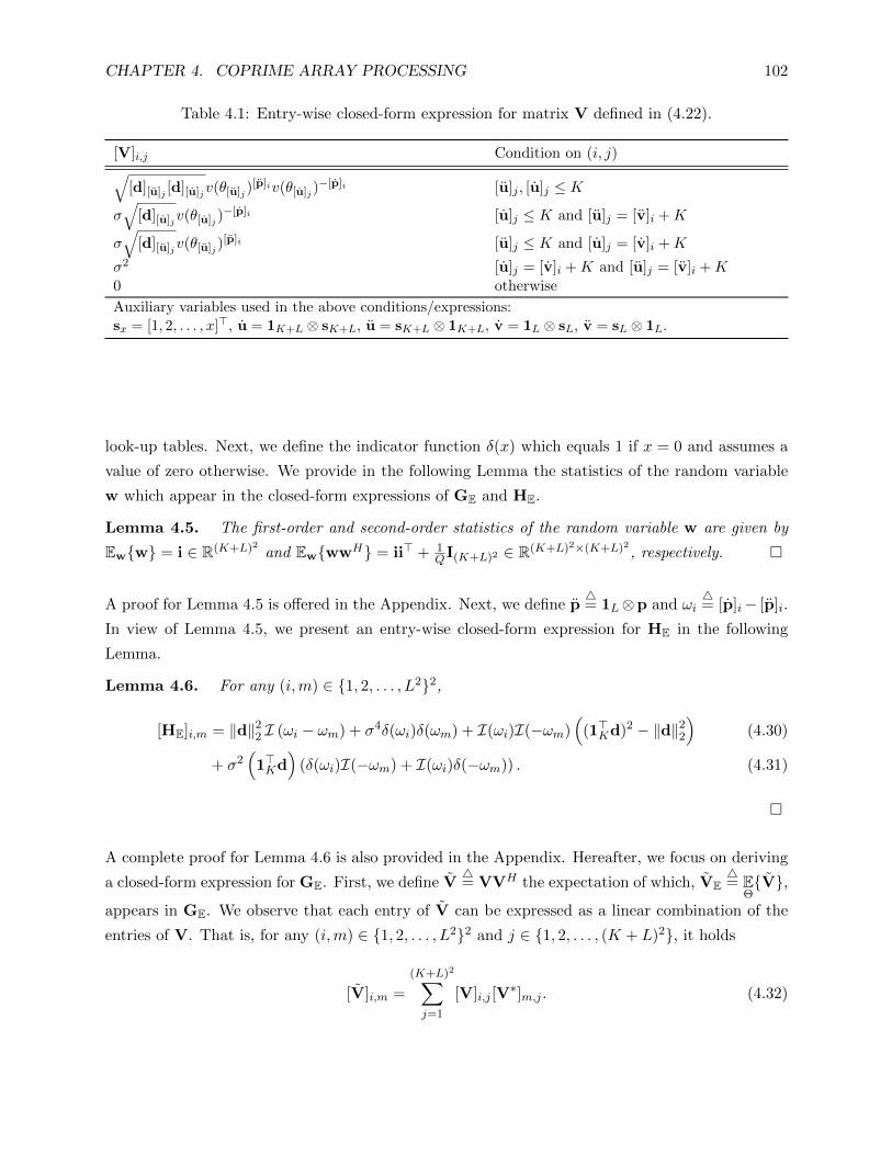
CHAPTER 4. COPRIME ARRAY PROCESSING 102
Table 4.1: Entry-wise closed-form expression for matrix V defined in (4.22).
[V]i,j Condition on (i, j)√[d][u]j [d][u]jv(θ[u]j )
[p]iv(θ[u]j )−[p]i [u]j , [u]j ≤ K
σ√
[d][u]jv(θ[u]j )−[p]i [u]j ≤ K and [u]j = [v]i +K
σ√
[d][u]jv(θ[u]j )[p]i [u]j ≤ K and [u]j = [v]i +K
σ2 [u]j = [v]i +K and [u]j = [v]i +K0 otherwise
Auxiliary variables used in the above conditions/expressions:sx = [1, 2, . . . , x]>, u = 1K+L ⊗ sK+L, u = sK+L ⊗ 1K+L, v = 1L ⊗ sL, v = sL ⊗ 1L.
look-up tables. Next, we define the indicator function δ(x) which equals 1 if x = 0 and assumes a
value of zero otherwise. We provide in the following Lemma the statistics of the random variable
w which appear in the closed-form expressions of GE and HE.
Lemma 4.5. The first-order and second-order statistics of the random variable w are given by
Eww = i ∈ R(K+L)2 and EwwwH = ii> + 1QI(K+L)2 ∈ R(K+L)2×(K+L)2, respectively.
A proof for Lemma 4.5 is offered in the Appendix. Next, we define p4= 1L⊗p and ωi
4= [p]i− [p]i.
In view of Lemma 4.5, we present an entry-wise closed-form expression for HE in the following
Lemma.
Lemma 4.6. For any (i,m) ∈ 1, 2, . . . , L22,
[HE]i,m = ‖d‖22 I (ωi − ωm) + σ4δ(ωi)δ(ωm) + I(ωi)I(−ωm)(
(1>Kd)2 − ‖d‖22)
(4.30)
+ σ2(1>Kd
)(δ(ωi)I(−ωm) + I(ωi)δ(−ωm)) . (4.31)
A complete proof for Lemma 4.6 is also provided in the Appendix. Hereafter, we focus on deriving
a closed-form expression for GE. First, we define V4= VVH the expectation of which, VE
4= E
ΘV,
appears in GE. We observe that each entry of V can be expressed as a linear combination of the
entries of V. That is, for any (i,m) ∈ 1, 2, . . . , L22 and j ∈ 1, 2, . . . , (K + L)2, it holds
[V]i,m =
(K+L)2∑j=1
[V]i,j [V∗]m,j . (4.32)

CHAPTER 4. COPRIME ARRAY PROCESSING 103
Table 4.2: Closed-form expression for γ(i,m)j defined in (4.33) .
γ(i,m)j Condition on (i,m, j)
[d][u]j [d][u]jv(θ[u]j ])[p]i−[p]mv(θ[u]j )
[p]m−[p]i [u]j=[u]j ≤ K,[d][u]j [d][u]jv(θ[u]j )
[p]i−[p]mv(θ[u]j )[p]m−[p]i [u]j , [u]j ≤ K; [u]j 6= [u]j
σ2[d][u]jv(θ[u]j )[p]m−[p]i [u]j ≤ K; [u]j−K=[v]i=[v]m
σ2[d][u]jv(θ[u]j )[p]i−[p]m [u]j ≤ K; [u]j−K=[v]i=[v]m
σ4 [u]j−K=[v]i=[v]m; [u]j−K=[v]i = [v]m0 otherwise
Auxiliary variables used in the above conditions/expressions:p = p⊗ 1L, p = 1L ⊗ p, sx = [1, 2, . . . , x]>, u = 1K+L ⊗ sK+L, u = sK+L ⊗ 1K+L, v = 1L ⊗ sL, v = sL ⊗ 1L.
Table 4.3: Closed-form expression for EΘγ(i,m)j .
Eθγ(i,m)j Condition on (i,m, j)
[d][u]j [d][u]jI(ωm,i + ωi,m) [u]j=[u]j ≤ K,[d][u]j [d][u]jI(ωm,i)I(ωi,m) [u]j , [u]j ≤ K; [u]j 6= [u]jσ2[d][u]jI(ωm,i) [u]j ≤ K; [u]j−K=[v]i=[v]mσ2[d][u]jI(ωi,m) [u]j ≤ K; [u]j−K=[v]i=[v]mσ4 [u]j−K=[v]i=[v]m; [u]j−K=[v]i = [v]m0 otherwiseAuxiliary variables used in the above conditions/expressions:p = p⊗ 1L, p = 1L ⊗ p, ωi,j = [p]i − [p]j , ωi,j = [p]i − [p]j , sx = [1, 2, . . . , x]>, u = 1K+L ⊗ sK+L, u = sK+L ⊗ 1K+L,v = 1L ⊗ sL, v = sL ⊗ 1L.
An entry-wise closed-form expression for V, in terms of Θ, is offered in Table 4.1. Then, for
any triplet (i,m, j) such that (i,m) ∈ 1, 2, . . . , L22 and j ∈ 1, 2, . . . , (K + L)2, we derive a
closed-form expression for
γ(i,m)j
4= [V]i,j [V
∗]m,j , (4.33)
in Table 4.2. Accordingly, EΘγ(i,m)j is offered in Table 4.3, based on which, the (i,m)th entry
of VE is computed as
[VE]i,m =
(K+L)2∑j=1
EΘγ(i,m)j . (4.34)
In view of the above, we offer a closed-form expression for matrix GE in the following Lemma.

CHAPTER 4. COPRIME ARRAY PROCESSING 104
Lemma 4.7. Matrix GE is given by GE = HE + 1QVE.
A proof for Lemma 4.7 is offered in the Appendix. Next, we differentiate (4.27) with respect to E,
set its derivative to zero, and obtain(HE +
1
QVE
)EMMSE = HEEsel. (4.35)
We observe that (4.35) is, in practice, a collection of (2L′ − 1) systems of linear equations. Let
EMMSE = [e1, . . . , e2L′−1] and ci = [HEEsel]:,i∀i ∈ 1, 2, . . . , 2L′ − 1. Solving (4.35) is equivalent
to solving, for every i,
GEei = ci. (4.36)
For any i such that ci ∈ span(GE), (4.36) has at least one exact solution ei = VΣ−1UHci + bi,
where GE admits SVD UL2×ρΣρ×ρVHρ×L2 , ρ = rank(GE), and bi is an arbitrary vector in the
nullspace of GE which is denoted by N (GE). In the special case that ρ = L2, that is, GE has
full-rank, then N (GE) = 0L2 and there exists a unique solution ei = VΣ−1UHci. If, on the other
hand, ∃i such that ci /∈ span(GE), then (4.36) does not have an exact solution and a Least Squares
(LS) approach can be followed by solving minei ‖GEei− ci‖22. Interestingly, it is easy to show that
the LS solution is the same as before –i.e., ei = VΣ−1UHci + bi, where bi ∈ N (GE). In every
case, each column of EMMSE can be computed in closed-form as
ei = VΣ−1UHci + bi, bi ∈ N (GE). (4.37)
In view of the above, we propose to process the autocorrelations in r by the linear combiner EMMSE
to obtain the MMSE estimate of rco,
rMMSE4= E>MMSEr. (4.38)
In turn, we propose to Minimum-MSE estimate Z in (4.6) by ZMMSE = Φ (rMMSE).
Next, we discuss the computational complexity of forming EMMSE. First, we consider the cost of
numerically approximating the integral I(x) in (4.28) for any DoA probability distribution f(θ),
support set (a, b), and scalar x. There is rich literature on theory, methods, and complexity/ac-
curacy trade-offs in numerical integration –a topic that extends well beyond the scope of this
article. For the purpose of our complexity analysis, we consider that I(x) can be approximated

CHAPTER 4. COPRIME ARRAY PROCESSING 105
within numerical error tolerance ε > 0 by, e.g., trapezoidal, midpoint, and Simpson’s interpolatory
quadrature rules [204–206], with cost O(C), where C = 1√ε. Next, we note that evaluating I(x) for
every x ∈ V 4= ωiL2
i=1 ∪ ωi − ωmL2
i,m=1 ∪ ωiL2
i=1 ∪ ωiL2
i=1 ∪ ωm,i + ωi,mL2
i,m=1 costs at most
O(MNC). Having computed I(x) for every x ∈ V, we can form matrices HE and VE with costs
O(L4) and O(L6 +KL5), respectively. Thereafter, the SVD of GE = HE + 1QVE for solving (4.36)
requires O(L6) computations. Observing that L = 2M + N − 1 and K ≤ MN + M and keeping
only the dominant terms, the computational complexity of forming EMMSE is O(L6 + MNC). In
addition, we note that the computation of I(x) for different values of x can be performed in paral-
lel, tremendously reducing the computation time. In this work, we conduct numerical integration
by means of the vectorized adaptive quadrature approach of [204] with absolute error tolerance
ε = 1e − 10. As a simple numerical example, for (M,N) = (2, 3), K = 7, ε = 1e − 10, and serial
computation of the numerical integrals, in MATLAB 2019a (generic software) running on an In-
tel(R) core(TM) i7-8700 processor at 3.2 GHz and 32GB RAM (generic hardware), we computed
EMMSE in a very small fraction of a second.
Finally, a remark is in order on the source powers and noise variance. The proposed linear combiner
EMMSE depends on HE and VE which, in turn, depend on the powers d1, d2, . . . , dK , σ2 associated
to the source DoAs θ1, θ2, . . . , θK and noise, respectively. In this Section, we assume the signal-
source powers and noise variance to be known. Joint power/DoA estimation is beyond the scope of
this Section. For the problem of the power estimation, we refer the interested reader to, e.g., the
works in [209–214].
4.5.1 Numerical Studies
We consider coprime naturals (M,N) with M < N and form a length-(L = 2M +N − 1) coprime
array which corresponds to a length-(L′ = MN +M) virtual ULA –i.e., the coarray. Signals from
K sources impinge on the array with equal transmit power d1 = d2 = ... = dK = α2 = 10dB. The
noise variance is set to σ2 = 0dB. Accordingly, the Signal-to-Noise-Ratio (SNR) is set to 10dB for
every DoA signal source.
We commence our studies by computing the empirical Cumulative Distribution Function (CDF)
of the Normalized-MSE (NMSE) in estimating Z for a given DoA collection Θ = θ1, . . . , θKsuch that the DoAs in Θ are i.i.d. –i.e., θk ∼ D(a, b)∀k. More specifically, we consider fixed
sample-support Q = 10 and for each estimate Z ∈ Zsel, Zavg, ZMMSE, we compute the estimation

CHAPTER 4. COPRIME ARRAY PROCESSING 106
0 0.5 1 1.5NMSE
0
0.2
0.4
0.6
0.8
1E
MP
IRIC
AL
CD
F
MMSE (proposed)AVERAGINGSELECTION
0 0.5 1 1.5NMSE
0
0.2
0.4
0.6
0.8
1
EM
PIR
ICA
L C
DF
MMSE (proposed)AVERAGINGSELECTION
0 0.5 1 1.5NMSE
0
0.2
0.4
0.6
0.8
1
EM
PIR
ICA
L C
DF
MMSE (proposed)AVERAGINGSELECTION
0 0.5 1 1.5NMSE
0
0.2
0.4
0.6
0.8
1
EM
PIR
ICA
L C
DF
MMSE (proposed)AVERAGINGSELECTION
0 0.5 1 1.5NMSE
0
0.2
0.4
0.6
0.8
1E
MP
IRIC
AL
CD
F
MMSE (proposed)AVERAGINGSELECTION
0 0.5 1 1.5NMSE
0
0.2
0.4
0.6
0.8
1
EM
PIR
ICA
L C
DF
MMSE (proposed)AVERAGINGSELECTION
Figure 4.7. Empirical CDF of the MSE in estimating Z for (M,N) = (2, 3), SNR= 10dB, Q = 10,K = 5 (top), and K = 7 (bottom). ∀k, θk ∼ U(−π
2 ,π2 ) (left), U(−π
4 ,π6 ) (center), T N (−π
8 ,π8 , 0, 1)
(right).
error
NMSE =∥∥∥Z− Z
∥∥∥2
F‖Z‖−2
F . (4.39)
We repeat this process over 4000 statistically independent realizations of Θ and AWGN. We collect
4000 NMSE measurements based on which we plot, in Fig. 4.7, the empirical CDF of the NMSE
in estimating Z for fixed (M,N) = (2, 3), K ∈ 5, 7, and
D(a, b) ∈ U(−π2,π
2),U(−π
4,π
6), T N(−π
8,π
8, 0, 1). (4.40)
We observe that the proposed MMSE combining approach attains superior MSE in estimating
Z for any distribution and support set considered for the DoAs in Θ. Moreover, we notice that
the averaging combining approach consistently outperforms the selection combining approach in
accordance with our theoretical finding that averaging combining attains superior performance

CHAPTER 4. COPRIME ARRAY PROCESSING 107
0 0.2 0.4 0.6 0.8 1NMSE
0
0.2
0.4
0.6
0.8
1E
MP
IRIC
AL
CD
F
MMSE (proposed)AVERAGINGSELECTION
0 0.2 0.4 0.6 0.8 1NMSE
0
0.2
0.4
0.6
0.8
1
EM
PIR
ICA
L C
DF
MMSE (proposed)AVERAGINGSELECTION
0 0.2 0.4 0.6 0.8 1NMSE
0
0.2
0.4
0.6
0.8
1
EM
PIR
ICA
L C
DF
MMSE (proposed)AVERAGINGSELECTION
0 0.2 0.4 0.6 0.8 1NMSE
0
0.2
0.4
0.6
0.8
1
EM
PIR
ICA
L C
DF
MMSE (proposed)AVERAGINGSELECTION
0 0.2 0.4 0.6 0.8 1NMSE
0
0.2
0.4
0.6
0.8
1E
MP
IRIC
AL
CD
F
MMSE (proposed)AVERAGINGSELECTION
0 0.2 0.4 0.6 0.8 1NMSE
0
0.2
0.4
0.6
0.8
1
EM
PIR
ICA
L C
DF
MMSE (proposed)AVERAGINGSELECTION
Figure 4.8. Empirical CDF of the NMSE in estimating Z for (M,N) = (2, 5), SNR= 10dB,Q = 10, K = 7 (top), and K = 9 (bottom). ∀k, θk ∼ U(−π
2 ,π2 ) (left), U(−π
4 ,π6 ) (center), and
T N (−π8 ,
π8 , 0, 1) (right).
compared to selection combining. Furthermore, we observe that the performance advantage of
the proposed MMSE combining approach over its standard counterparts is more emphatic when
θk ∼ U(−π4 ,
π6 ). Last, we notice that for θk ∼ U(−π
4 ,π6 ), the performance gap between the proposed
MMSE combining and the standard averaging approach is greater for K = 7. We repeat the last
study for (M,N) = (2, 5), K ∈ 7, 9, and D(a, b) ∈ U(−π2 ,
π2 ),U(−π
4 ,π6 ), T N(−π
8 ,π8 , 0, 1). We
illustrate the new CDFs in Fig. 4.8. Similar observations as in Fig. 4.7 are made. The proposed
MMSE combining approach clearly outperforms its standard counterparts for any distribution
assumption and support set for θk∀k.
For fixed K = 7 and every other parameter same as above, we plot the NMSE (averaged over
4000 realizations) versus sample support Q ∈ 1, 10, 100, 1000, 10000, in Fig. 4.9. Consistent
with the observations above, we notice that selection attains the highest NMSE while the proposed
MMSE combiner attains, expectedly, the lowest NMSE in estimating Z across the board. The
performance gap between the proposed MMSE combining estimate and the estimates based on

CHAPTER 4. COPRIME ARRAY PROCESSING 108
100 102 104
Sample support, Q
10-4
10-2
100
NM
SE
MMSE (proposed)AVERAGINGSELECTION
100 102 104
Sample support, Q
10-4
10-2
100
NM
SE
MMSE (proposed)AVERAGINGSELECTION
100 102 104
Sample support, Q
10-4
10-2
100
NM
SE
MMSE (proposed)AVERAGINGSELECTION
Figure 4.9. NMSE in estimating Z, versus sample support, Q. (M,N) = (2, 5), SNR= 10dB, andK = 7. ∀k, θk ∼ U(−π
2 ,π2 ) (left), U(−π
4 ,π6 ) (center), T N (−π
8 ,π8 , 0, 1) (right).
100 102 104
Sample support, Q
18
20
22
24
RM
SE
(de
g.)
MMSE (proposed)AVERAGINGSELECTION
100 102 104
Sample support, Q
8
9
10
11
12
13
RM
SE
(de
g.)
MMSE (proposed)AVERAGINGSELECTION
100 102 104
Sample support, Q
5
6
7
8
RM
SE
(de
g.)
MMSE (proposed)AVERAGINGSELECTION
Figure 4.10. RMSE (degrees) in estimating the DoA set Θ, versus sample support, Q. (M,N) =(2, 5), SNR= 10dB, and K = 7. ∀k, θk ∼ U(−π
2 ,π2 ) (left), U(−π
4 ,π6 ) (center), T N (−π
8 ,π8 , 0, 1)
(right).
existing combining approaches decreases as the sample support Q increases. Nonetheless, it remains
superior, in many cases, even for high values of Q –e.g., Q = 104. Moreover, in the first two subplots
(uniform DoA distribution), we notice that the performance gap between the MMSE combining
approach and the averaging approach is wider when the range of the support set (a, b) is narrower.
Next, we evaluate the performance of the proposed MMSE combining approach and its counterparts
by measuring the Root-MSE (RMSE) in estimating the DoAs in Θ versus sample support Q. First,
we evaluate the MUSIC spectrum for each estimate Z ∈ Zsel, Zavg, ZMMSE over the probability
distribution support set (a, b) and obtain DoA estimates in Θ = θ1, . . . , θK. Then, we compute

CHAPTER 4. COPRIME ARRAY PROCESSING 109
100 102 104
Sample support, Q
10-2
10-1
100
101R
MS
E (
deg.
)
MMSE (proposed)AVERAGINGSELECTIONCRLB
1 106
11
100 102 104
Sample support, Q
10-2
10-1
100
101
RM
SE
(de
g.)
MMSE (proposed)AVERAGINGSELECTIONCRLB
100 102 104
Sample support, Q
10-2
10-1
100
101
RM
SE
(de
g.)
MMSE (proposed)AVERAGINGSELECTIONCRLB
100 102 104
Sample support, Q
10-2
10-1
100
101
RM
SE
(de
g.)
MMSE (proposed)AVERAGINGSELECTIONCRLB
1 105
11
100 102 104
Sample support, Q
10-2
100
RM
SE
(de
g.)
MMSE (proposed)AVERAGINGSELECTIONCRLB
100 102 104
Sample support, Q
10-2
10-1
100
101
RM
SE
(de
g.)
MMSE (proposed)AVERAGINGSELECTIONCRLB
Figure 4.11. RMSE (degrees) in estimating the DoA set Θ, versus sample support, Q. (M,N) =(3, 5) and K = 11. (Θ,SNR,D(a, b)) = (Θ1, 0dB,U(−π
2 ,π2 )) –top left, (Θ1, 8dB,U(−π
2 ,π2 )) –bottom
left, (Θ2, 0dB,U(−π4 ,
π4 )) –top center, (Θ2, 8dB,U(−π
4 ,π4 )) –bottom center, (Θ3, 0dB,U(−π
4 ,π6 )) –
top right, (Θ3, 8dB,U(−π4 ,
π6 )) –bottom right.
the estimation error
MSE(Θ) =1
K
K∑k=1
(θk − θk)2. (4.41)
We compute the RMSE by taking the square root of the MSE(Θ) computed over 4000 statistically
independent realizations of Θ and AWGN. The resulting RMSE curves are depicted in Fig. 4.10.
For every DoA distribution (even the most general case of uniform distribution in (−π2 ,
π2 )) and
every sample support (even as high as 104), the proposed method attains the lowest RMSE.
We conclude our studies by evaluating the DoA estimation performance of the proposed MMSE
combiner and its counterparts for fixed DoAs. This time, we consider coprime naturals (M,N) =
(3, 5) forming an array with L = 10 sensors, fixed number of sources K = 11, and three distinct

CHAPTER 4. COPRIME ARRAY PROCESSING 110
realizations of DoA set Θ = θ1, . . . , θK:
Θ1 = −79,−55,−43,−25,−15,−6, 7, 21, 34, 54, 63, (4.42)
Θ2 = −44,−38,−27,−12,−3, 6, 17, 24, 31, 37, 44, (4.43)
Θ3 = −44,−37,−31,−23,−15,−8,−2, 4, 17, 22, 29. (4.44)
For every fixed Θi, i ∈ 1, 2, 3, we proceed as follows in order to compute the RMSE curves.
First, we consider 4000 statistically independent realizations of AWGN for SNR ∈ 0, 8dB. For
every realization, we compute DoA estimate Θi as previously described and evaluate the MUSIC
spectrum over a probability distribution support set. We then measure MSE(Θi) as described above
and compute the RMSE by taking the square root of the sample-average of the 4000 MSE(Θi)
measurements. As a benchmark, we also compute the Cramer Rao Lower Bound (CRLB) curves
computed by means of the closed-form expression that follows, first derived in [165], as2
CRLBΘ =1
Q
(MH
Θ ΠMΘ
)−1, (4.45)
where
MΘ = (R>y ⊗Ry)− 1
2 Sddiag(d), (4.46)
Π = IL2 −Ms(MHs Ms)
−1MHs , (4.47)
Ms = (R>y ⊗Ry)− 1
2 [Sd vec(IL)], (4.48)
Sd = S∗ S, (4.49)
Sd = S∗ S + S∗ S, (4.50)
S = [∂s(θ1)
∂θ1, . . . ,
∂s(θK)
∂θK]. (4.51)
In Fig. 4.11 (left), we plot the RMSE and CRLB curves versus sample support for Θ = Θ1, and
SNR= 0dB (top-left) and SNR= 8dB (bottom-left), respectively. We form the MMSE combiner
by considering D(a, b) = U(−π2 ,
π2 ). We observe that for SNR ∈ 0, 8dB and low sample support,
Q ≤ 100, the proposed MMSE combiner clearly outperforms its counterparts in DoA estimation
accuracy. For Q ≥ 1000, the proposed MMSE and the averaging combiners attain almost identical
performance, superior to that of the selection combiner.
In Fig. 4.11 (center), we plot the RMSE and CRLB curves versus sample support for Θ = Θ2,
and SNR= 0dB (top-center) and SNR= 8dB (bottom-center), respectively. We consider D(a, b) =
2Operator ‘’ denotes the column-wise Kronecker product of matrices, also known as Khatri-Rao product.
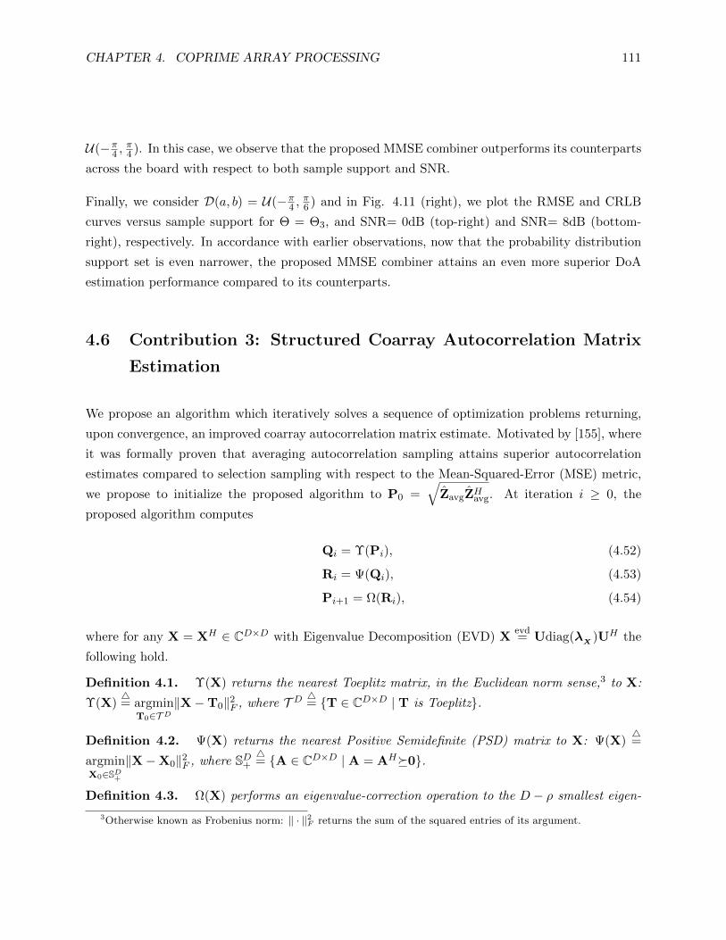
CHAPTER 4. COPRIME ARRAY PROCESSING 111
U(−π4 ,
π4 ). In this case, we observe that the proposed MMSE combiner outperforms its counterparts
across the board with respect to both sample support and SNR.
Finally, we consider D(a, b) = U(−π4 ,
π6 ) and in Fig. 4.11 (right), we plot the RMSE and CRLB
curves versus sample support for Θ = Θ3, and SNR= 0dB (top-right) and SNR= 8dB (bottom-
right), respectively. In accordance with earlier observations, now that the probability distribution
support set is even narrower, the proposed MMSE combiner attains an even more superior DoA
estimation performance compared to its counterparts.
4.6 Contribution 3: Structured Coarray Autocorrelation Matrix
Estimation
We propose an algorithm which iteratively solves a sequence of optimization problems returning,
upon convergence, an improved coarray autocorrelation matrix estimate. Motivated by [155], where
it was formally proven that averaging autocorrelation sampling attains superior autocorrelation
estimates compared to selection sampling with respect to the Mean-Squared-Error (MSE) metric,
we propose to initialize the proposed algorithm to P0 =√
ZavgZHavg. At iteration i ≥ 0, the
proposed algorithm computes
Qi = Υ(Pi), (4.52)
Ri = Ψ(Qi), (4.53)
Pi+1 = Ω(Ri), (4.54)
where for any X = XH ∈ CD×D with Eigenvalue Decomposition (EVD) Xevd= Udiag(λX )UH the
following hold.
Definition 4.1. Υ(X) returns the nearest Toeplitz matrix, in the Euclidean norm sense,3 to X:
Υ(X)4= argmin
T0∈T D‖X−T0‖2F , where T D 4= T ∈ CD×D | T is Toeplitz.
Definition 4.2. Ψ(X) returns the nearest Positive Semidefinite (PSD) matrix to X: Ψ(X)4=
argminX0∈SD+
‖X−X0‖2F , where SD+4= A ∈ CD×D | A = AH0.
Definition 4.3. Ω(X) performs an eigenvalue-correction operation to the D − ρ smallest eigen-
3Otherwise known as Frobenius norm: ‖ · ‖2F returns the sum of the squared entries of its argument.
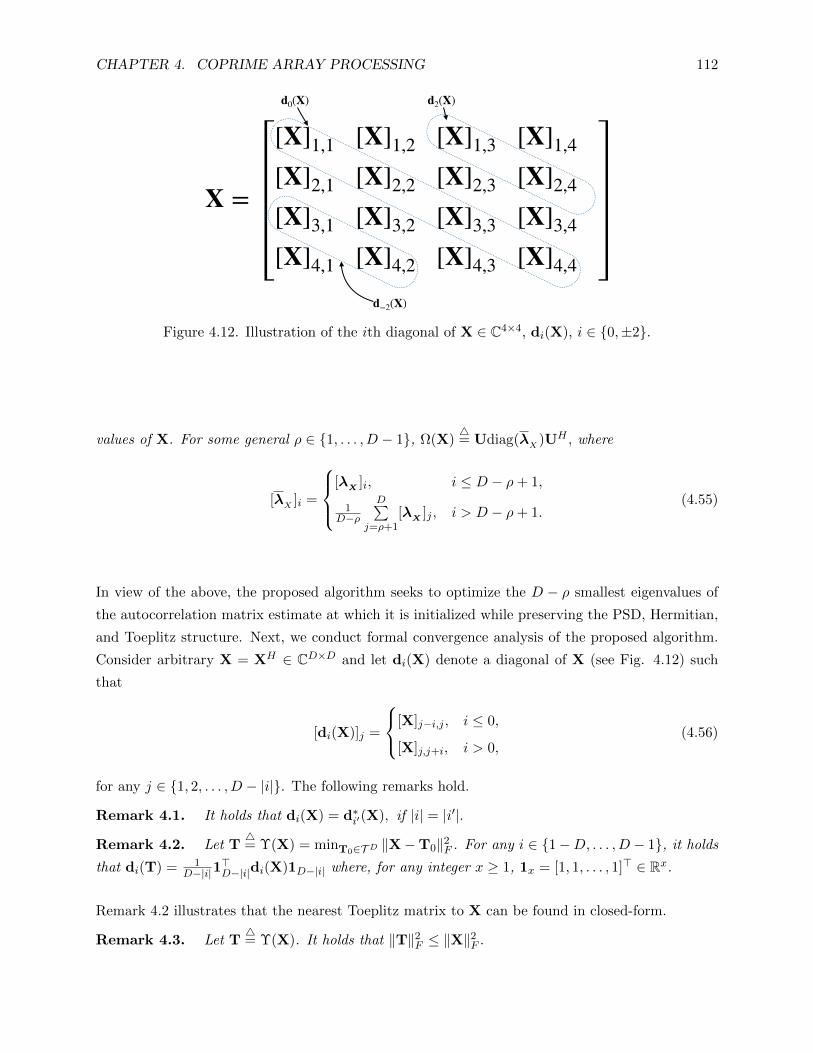
CHAPTER 4. COPRIME ARRAY PROCESSING 112
X =[X]1,1 [X]1,2 [X]1,3 [X]1,4[X]2,1 [X]2,2 [X]2,3 [X]2,4[X]3,1 [X]3,2 [X]3,3 [X]3,4[X]4,1 [X]4,2 [X]4,3 [X]4,4
d0(X) d2(X)
d−2(X)Figure 4.12. Illustration of the ith diagonal of X ∈ C4×4, di(X), i ∈ 0,±2.
values of X. For some general ρ ∈ 1, . . . , D − 1, Ω(X)4= Udiag(λX )UH , where
[λX ]i =
[λX ]i, i ≤ D − ρ+ 1,
1D−ρ
D∑j=ρ+1
[λX ]j , i > D − ρ+ 1.(4.55)
In view of the above, the proposed algorithm seeks to optimize the D − ρ smallest eigenvalues of
the autocorrelation matrix estimate at which it is initialized while preserving the PSD, Hermitian,
and Toeplitz structure. Next, we conduct formal convergence analysis of the proposed algorithm.
Consider arbitrary X = XH ∈ CD×D and let di(X) denote a diagonal of X (see Fig. 4.12) such
that
[di(X)]j =
[X]j−i,j , i ≤ 0,
[X]j,j+i, i > 0,(4.56)
for any j ∈ 1, 2, . . . , D − |i|. The following remarks hold.
Remark 4.1. It holds that di(X) = d∗i′(X), if |i| = |i′|.
Remark 4.2. Let T4= Υ(X) = minT0∈T D ‖X−T0‖2F . For any i ∈ 1−D, . . . ,D − 1, it holds
that di(T) = 1D−|i|1
>D−|i|di(X)1D−|i| where, for any integer x ≥ 1, 1x = [1, 1, . . . , 1]> ∈ Rx.
Remark 4.2 illustrates that the nearest Toeplitz matrix to X can be found in closed-form.
Remark 4.3. Let T4= Υ(X). It holds that ‖T‖2F ≤ ‖X‖2F .
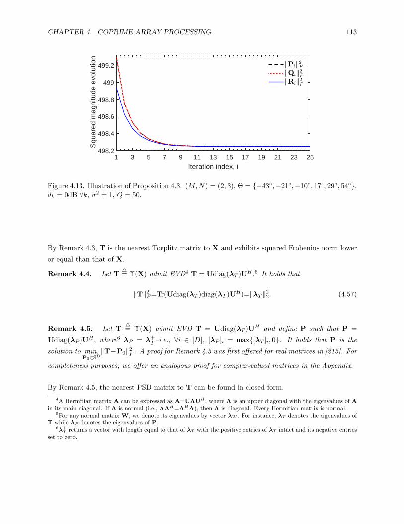
CHAPTER 4. COPRIME ARRAY PROCESSING 113
1 3 5 7 9 11 13 15 17 19 21 23 25
Iteration index, i
498.2
498.4
498.6
498.8
499
499.2
Squ
ared
mag
nitu
de e
volu
tion
Figure 4.13. Illustration of Proposition 4.3. (M,N) = (2, 3), Θ = −43,−21,−10, 17, 29, 54,dk = 0dB ∀k, σ2 = 1, Q = 50.
By Remark 4.3, T is the nearest Toeplitz matrix to X and exhibits squared Frobenius norm lower
or equal than that of X.
Remark 4.4. Let T4= Υ(X) admit EVD4 T = Udiag(λT )UH .5 It holds that
‖T‖2F=Tr(Udiag(λT )diag(λT )UH)=‖λT ‖22. (4.57)
Remark 4.5. Let T4= Υ(X) admit EVD T = Udiag(λT )UH and define P such that P =
Udiag(λP )UH , where6 λP = λ+T –i.e., ∀i ∈ [D], [λP ]i = max[λT ]i, 0. It holds that P is the
solution to min.P0∈SD+
‖T−P0‖2F . A proof for Remark 4.5 was first offered for real matrices in [215]. For
completeness purposes, we offer an analogous proof for complex-valued matrices in the Appendix.
By Remark 4.5, the nearest PSD matrix to T can be found in closed-form.
4A Hermitian matrix A can be expressed as A=UΛUH , where Λ is an upper diagonal with the eigenvalues of Ain its main diagonal. If A is normal (i.e., AAH=AHA), then Λ is diagonal. Every Hermitian matrix is normal.
5For any normal matrix W, we denote its eigenvalues by vector λW . For instance, λT denotes the eigenvalues ofT while λP denotes the eigenvalues of P.
6λ+T returns a vector with length equal to that of λT with the positive entries of λT intact and its negative entries
set to zero.

CHAPTER 4. COPRIME ARRAY PROCESSING 114
Input: Coarray autocorrelation matrix estimate ROutput: R ← Pi
P0 ← R % Initialization
Until convergence/terminationQi ← Υ(Pi) % Nearest Toeplitz to Pi
Ri ← Ψ(Qi) % Nearest PSD to Qi
Pi+1 ← Ω(Ri) % Eigenvalue-correction
Algorithm 4.1 Structured coarray autocorrelation matrix estimation
Remark 4.6. For P = Ψ(T), it holds that ‖P‖2F ≤ ‖T‖2F . Formally,
‖P‖2F=‖λP ‖22 =D∑i=1
[λP ]2i ≤D∑i=1
[λT ]2i = ‖T‖2F (4.58)
By Remark 4.6, P is the nearest PSD matrix to T and attains squared Frobenius norm lower or
equal than that of T.
Remark 4.7. Let A = Ω(P) = Udiag(λA)UH , where
[λA]i =
[λP ]i, i ≤ D − ρ+ 1,
1D−ρ
D∑j=ρ+1
[λP ]j , i > D − ρ+ 1,(4.59)
for ρ ∈ 1, . . . , D − 1. It holds that ‖A‖2F ≤ ‖P‖2F .
By Remark 4.7, the eigenvalue correction operation on a normal matrix returns a matrix with
squared-Frobenius norm lower or equal than that of its input argument. In view of Remarks
4.1-4.7, the following Proposition derives.
Proposition 4.3. For Qi,Ri, and Pi+1 in (4.52)-(4.54), it holds that
‖Qi‖2F ≥ ‖Ri‖2F ≥ ‖Pi+1‖2F ≥ ‖Qi+1‖2F ≥ . . . ≥ 0∀i ≥ 0. (4.60)
Proposition 4.3 states that the proposed algorithm is guaranteed to converge. In practice, one can
terminate the iterations when ‖Pi+1−Pi‖ ≤ ε, for some ε ≥ 0. For sufficiently small ε, Proposition 1

CHAPTER 4. COPRIME ARRAY PROCESSING 115
Matrix estimate Autocorrelation sampling approach Positive Definite Toeplitz Hermitian Equal noise-subspace eigenvalues
Zsel Selection 7 3 3 7
Zavg Averaging 7 3 3 7
Zpsr Averaging 3 7 3 7
Structured (proposed) Averaging 3 3 3 3
Table 4.4: Comparison of coarray autocorrelation matrix estimates: autocorrelation sampling ap-proach and structure properties.
implies that, at convergence, Pi+1 = Ri = Qi which, in turn, implies that the algorithm converged
to a PD, Hermitian, and Toeplitz matrix the noise-subspace eigenvalues of which are equal. A
visual illustration of Proposition 4.3 and a pseudocode of the proposed algorithm are offered in Fig.
4.13 and Algorithm 4.1, respectively. Importantly, ∀i ≥ 0, the Algorithm of Fig. 4.14 computes
Qi,Ri,Pi+1 by closed-form expressions with cost at most the cost of EVD–i.e., O(D3). Overall,
the cost of the proposed algorithm is O(TD3) where T is the number of iterations required for
convergence.
We summarize the above estimates in Table 4.4, where for each estimate we mention the employed
autocorrelation sampling approach. Moreover, for each structure property guaranteed to be sat-
isfied, we place a ‘3’, otherwise, we place a ‘7’. Given a coarray autocorrelation matrix estimate
R ∈ Zsel, Zavg, Zpsr, a standard DoA estimation approach –e.g., MUltiple SIgnal Classification
(MUSIC) –is applied for identifying the DoAs in Θ.
4.6.1 Numerical Studies
We consider coprime naturals (M,N) = (3, 5) and form coprime array with L = 10 elements.
Source-signals impinge on the array from K = 13 DoAs θk13k=1, θk = (−75+(k−1)12). The noise
variance is set to σ2 = 0dB. All sources emit signals with equal power dk = α2dB. Accordingly,
the Signal-to-Noise Ratio SNR = α2. The receiver collects Q ∈ 150, 300, 450, 600 received-
signal snapshots. For every Q, we consider Γ = 3000 statistically independent realizations of
noise; i.e., yr,1, . . . ,yr,QΓr=1. At every realization r, we compute coarray autocorrelation matrix
estimates corresponding to the augmented matrix approach (AM), principal square root of the
spatial smoothed matrix (PSR), nearest Hermitian, PSD, and Toeplitz (H-PSD-T) approach of
[180]7, and the proposed structured estimate. We take a moment and discuss similarities and
7H-PSD-T seeks a Hermitian-PSD-Toeplitz matrix which fills the gaps of the coarray. When the uniform segmentof the coarray is considered, H-PSD-T returns argmin
R∈SL′+
‖R− Zavg‖2F+µ‖R‖∗, where µ‖R‖∗ is a regularization term
that moderates overfitting.
CHAPTER 4. COPRIME ARRAY PROCESSING 116
differences between H-PSD-T and the proposed framework: (1) H-PSD-T is guaranteed to satisfy
the Toeplitz, Hermitian, and Positive Semidefinite structure properties while the proposed estimate
is guaranteed to satisfy all four, (2) H-PSD-T requires tuning of an ad-hoc parameter that moderates
overfitting while the proposed framework is ad-hoc parameter free, and (3) H-PSD-T computes an
estimate by iterative solvers for convex optimization problems while the proposed approach enjoys
closed-form solutions for each individual optimization problem in its sequence. For every method
and estimate Rr at realization r, we compute the Normalized Squared Error
NSE(Rr) = ‖Rr − Z‖2F ‖Z‖−2F . (4.61)
Then, we compute the Root Mean Normalized Squared Error
RMNSE =
√√√√ 1
Γ
Γ∑r=1
NSE(Rr). (4.62)
In Fig. 4.15a and Fig. 4.15d, we plot the RMNSE versus sample support, Q, for SNR = −4dB and
SNR = 2dB, respectively. Expectedly, we observe that all methods employing averaging-sampling
perform similarly well. The proposed estimate attains superior estimation performance across the
board. Moreover, we notice the sensitivity of H-PSD-T with respect to the ad-hoc parameter µ; e.g.,
for SNR = −4dB, H-PSD-T with µ = 1.5 exhibits low performance while for SNR = 2dB it exhibits
high estimation performance. Thereafter, we consider that the nominal coarray autocorrelation
matrix admits SVD Z = QcoΣcoVHco + σ2QcoQ
Hco, where Qco and Qco correspond to the signal
and noise subspace bases, respectively. Similarly, every coarray autocorrelation matrix estimate
Rr admits SVD Rr = QrΣrVHr + QrΣrV
Hr , where Qr denotes the signal-subspace-basis of the K
dominant left-hand singular valued singular vectors of Rr. At each realization and for every value
of Q, we compute the Normalized Squared Subspace Error
NSSE(Qr) = ‖QrQHr −QcoQ
Hco‖2F (2K)−1. (4.63)
Then, we compute the Root Mean Normalized Squared Subspace Error
RMN-SSE =
√√√√ 1
Γ
Γ∑r=1
NSSE(Qr). (4.64)
In Fig. 4.15b and Fig. 4.15e, we plot the RMN-SSE versus sample support for SNR = −4dB and
2dB, respectively. We notice the influence of the ad-hoc parameter µ with respect to H-PSD-T
and observe that the proposed structured estimate clearly outperforms all counterparts across the

CHAPTER 4. COPRIME ARRAY PROCESSING 117
150 300 450 600Sample support, Q
0.1
0.15
0.2
0.25
0.3
RM
NS
EProposedAM w/ selectionAM w/ averagingPSR w/ averagingH-PSD-T w/ averaging =0.1H-PSD-T w/ averaging =1.5
(a) SNR = −4dB.
150 300 450 600Sample support, Q
0.05
0.1
0.15
0.2
RM
N-S
SE
ProposedAM w/ selectionAM w/ averagingPSR w/ averagingH-PSD-T w/ averaging =0.1H-PSD-T w/ averaging =1.5
(b) SNR = −4dB.
150 300 450 600Sample support, Q
0
2
4
6
8
RM
SE
(de
gree
s)
ProposedAM w/ selectionAM w/ averagingPSR w/ averagingH-PSD-T w/ averaging =0.1H-PSD-T w/ averaging =1.5CRLB
(c) SNR = −4dB.
150 300 450 600Sample support, Q
0.1
0.15
0.2
0.25
0.3
RM
NS
E
ProposedAM w/ selectionAM w/ averagingPSR w/ averagingH-PSD-T w/ averaging =0.1H-PSD-T w/ averaging =1.5
(d) SNR = 2dB.
150 300 450 600Sample support, Q
0.05
0.1
0.15
0.2
RM
N-S
SE
ProposedAM w/ selectionAM w/ averagingPSR w/ averagingH-PSD-T w/ averaging =0.1H-PSD-T w/ averaging =1.5
(e) SNR = 2dB.
150 300 450 600Sample support, Q
0
2
4
6
8
RM
SE
(de
gree
s)
ProposedAM w/ selectionAM w/ averagingPSR w/ averagingH-PSD-T w/ averaging =0.1H-PSD-T w/ averaging =1.5CRLB
(f) SNR = 2dB.
Figure 4.15. Root Mean Normalized Squared Error (RMNSE) with respect to (w.r.t.) Rco, RootMean Normalized - Subspace Squared Error (RMN-SSE) w.r.t. Qco, and Root Mean Squared Error(RMSE) w.r.t. Θ vs sample support for varying SNR ∈ −4, 2dB.
board in subspace estimation performance.
Next, for every value of sample support and realization r, we conduct DoA estimation by applying
MUSIC on the estimate Rr which returns estimates θk,rKk=1 [155]. Then, we measure the Root
Mean Squared Error
RMSE =
√√√√ 1
Γ
1
K
Γ∑r=1
K∑k=1
(θk − θk,r)2 (4.65)
and illustrate the corresponding RMSE curves versus sample support Q, in Fig. 4.15c and Fig.
4.15f, for SNR = −4dB and 2dB, respectively. We include the Cramer Rao Lower Bound (CRLB)
curves as benchmarks [165]. We notice that the the performances of standard counterparts (AM,
PSR) deviate significantly from the CRLB. In contrast, the proposed coarray autocorrelation matrix
estimate outperforms all counterparts by at least 0.3 and at most 2. In addition, as Q increases,
its performance curves approach the CRLB curves.
CHAPTER 4. COPRIME ARRAY PROCESSING 118
4.7 Conclusions
In this Chapter, we developed theory and novel algorithms for robust coprime array processing.
Specifically: (i) We derived closed-form MSE expressions for the estimation error attained by se-
lection and averaging autocorrelation combining and formally established the superiority of the
latter. The derived expressions are validated by means of numerical simulations. (ii) We proposed
a novel coprime array receiver that attains minimum MSE in coarray autocorrelation estimation,
for any probability distribution of the source DoAs. Extensive numerical studies on various DoA
distributions demonstrate that the proposed MMSE combining method consistently outperforms its
existing counterparts in autocorrelation estimation performance with respect to the MSE metric.
In turn, the proposed MMSE combiner enables lower RMSE in DoA estimation. (iii) We proposed
an optimization framework which computes a structured coarray autocorrelation matrix estimate.
The proposed algorithm is accompanied by convergence analysis and is guaranteed to return a coar-
ray autocorrelation matrix estimate satisfying all structure properties of the true autocorrelation
matrix. Numerical studies illustrate the enhanced performance of the proposed estimate compared
to standard counterparts, both in autocorrelation matrix estimation error and DoA estimation.
Bibliography
[1] L. R. Tucker, “Some mathematical notes on three-mode factor analysis,” Psychometrika,
vol. 31, no. 3, pp. 279–311, 1966, publisher: Springer.
[2] M. B. Amin, W. Zirwas, and M. Haardt, “HOSVD-Based Denoising for Improved Chan-
nel Prediction of Weak Massive MIMO Channels,” in IEEE Veh. Technol. Conf., Sydney,
Australia, Jun. 2017, pp. 1–5.
[3] D. C. Arajo, A. L. F. d. Almeida, J. P. C. L. D. Costa, and R. T. d. Sousa, “Tensor-Based
Channel Estimation for Massive MIMO-OFDM Systems,” IEEE Access, vol. 7, pp. 42 133–
42 147, 2019.
[4] W. D. C. Freitas, G. Favier, and A. L. De Almeida, “Tensor-Based Joint Channel and Symbol
Estimation for Two-Way MIMO Relaying Systems,” IEEE Signal Process. Lett., vol. 26, no. 2,
pp. 227–231, 2019.
[5] P. R. Gomes, A. L. de Almeida, and J. P. C. da Costal, “Fourth-order tensor method for blind
spatial signature estimation,” in 2014 IEEE International Conference on Acoustics, Speech
and Signal Processing (ICASSP). IEEE, 2014, pp. 2992–2996.
[6] H. Q. Ngo and E. G. Larsson, “EVD-based channel estimation in multicell multiuser MIMO
systems with very large antenna arrays,” in IEEE Int. Conf. Acoust., Speech Signal Process.,
Kyoto, Japan, Mar. 2012, pp. 3249–3252.
[7] P. Comon, “Tensors: a brief introduction,” IEEE Signal Process. Mag., vol. 31, no. 3, pp.
44–53, 2014.
[8] E. E. Papalexakis, C. Faloutsos, and N. D. Sidiropoulos, “Tensors for data mining and data
fusion: Models, applications, and scalable algorithms,” ACM Trans. Intell. Syst. Technol.,
vol. 8, pp. 16:1–16:44, Jan. 2017.
119

BIBLIOGRAPHY 120
[9] J. Kossaifi, Y. Panagakis, A. Anandkumar, and M. Pantic, “Tensorly: Tensor learning in
python,” J. Mach. Learn. Res., vol. 20, no. 1, pp. 925–930, 2019.
[10] G. G. Calvi, A. Moniri, M. Mahfouz, Z. Yu, Q. Zhao, and D. P. Mandic, “Tucker Tensor
Layer in Fully Connected Neural Networks,” arXiv preprint arXiv:1903.06133, 2019.
[11] J. Gusak, M. Kholyavchenko, E. Ponomarev, L. Markeeva, I. Oseledets, and A. Cichocki,
“One time is not enough: iterative tensor decomposition for neural network compression,”
arXiv preprint arXiv:1903.09973, 2019.
[12] N. D. Sidiropoulos, D. L. L, F. X, K. Huang, P. E. E, and F. C, “Tensor decomposition for
signal processing and machine learning,” IEEE Trans. Signal Process., vol. 65, no. 13, pp.
3551–3582, Jul. 2017.
[13] D. Tao, X. Li, W. Hu, S. Maybank, and X. Wu, “Supervised tensor learning,” in IEEE Int.
Conf. Data Mining, Houston, TX, Nov. 2005, pp. 8–pp.
[14] J. Kossaifi, Z. C. Lipton, A. Kolbeinsson, A. Khanna, T. Furlanello, and A. Anandkumar,
“Tensor regression networks,” J. Mach. Learn. Res., vol. 21, no. 123, pp. 1–21, 2020.
[15] A. Cichocki, D. Mandic, L. D. Lathauwer, G. Zhou, Q. Zhao, C. Caiafa, and H. A. Phan,
“Tensor Decompositions for Signal Processing Applications: From two-way to multiway com-
ponent analysis,” IEEE Signal Process. Mag., vol. 32, no. 2, pp. 145–163, 2015.
[16] M. A. O. Vasilescu and D. Terzopoulos, “Multilinear analysis of image ensembles: Tensor-
faces,” in European conference on computer vision. Springer, 2002, pp. 447–460.
[17] L. De Lathauwer, B. De Moor, and J. Vandewalle, “A multilinear singular value decomposi-
tion,” SIAM J. Matrix Anal. Appl., vol. 21, pp. 1253–1278, 2000.
[18] J. Yang, D. Zhang, A. F. Frangi, and J.-Y. Yang, “Two-dimensional PCA: a new approach
to appearance-based face representation and recognition,” IEEE Trans. Pattern Anal. Mach.
Intell., vol. 26, no. 1, pp. 131–137, 2004.
[19] R. Ballester-Ripoll, P. Lindstrom, and R. Pajarola, “TTHRESH: Tensor Compression for
Multidimensional Visual Data,” IEEE Trans. Vis. Comput. Graphics, pp. 2891–2903, 2019.
[20] H. Ben-Younes, R. Cadene, M. Cord, and N. Thome, “Mutan: Multimodal tucker fusion for
visual question answering,” in Proc. IEEE Int. Conf. Comput. Vision, Venice, Italy, Oct.
2017, pp. 2612–2620.

BIBLIOGRAPHY 121
[21] M. Mrup, L. K. Hansen, and S. M. Arnfred, “Algorithms for sparse nonnegative Tucker
decompositions,” Neural computation, vol. 20, no. 8, pp. 2112–2131, 2008, publisher: MIT
Press.
[22] J. Sun, S. Papadimitriou, C.-Y. Lin, N. Cao, S. Liu, and W. Qian, “Multivis: Content-based
social network exploration through multi-way visual analysis,” in Proceedings of the 2009
SIAM International Conference on Data Mining. SIAM, 2009, pp. 1064–1075.
[23] T. G. Kolda and J. Sun, “Scalable tensor decompositions for multi-aspect data mining,” in
2008 Eighth IEEE international conference on data mining. IEEE, 2008, pp. 363–372.
[24] C. M. Bishop, Pattern recognition and machine learning. Springer, 2006.
[25] R. O. Duda, P. E. Hart, and D. G. Stork, Pattern classification. John Wiley & Sons, 2012.
[26] A. Koochakzadeh and P. Pal, “On canonical polyadic decomposition of overcomplete ten-
sors of arbitrary even order,” in Proc. IEEE Int. Workshop Comput. Advances Multi-Sensor
Adaptive Process., Curaao, Dutch Antilles, Dec. 2017, pp. 1–5.
[27] A. Prater, “Classification via tensor decompositions of echo state networks,” in Proc. IEEE
Symp. Series Comput. Intell., Honolulu, HI, Dec. 2017, pp. 1–8.
[28] J. Ye, “Generalized low rank approximations of matrices,” Mach. Learn., vol. 61, pp. 167–191,
Nov. 2005.
[29] B. N. Sheehan and Y. Saad, “Higher order orthogonal iteration of tensors (HOOI) and its
relation to PCA and GLRAM,” in Proc. SIAM Int. Conf. Data Mining, Minneapolis, MN,
Apr. 2007, pp. 355–365.
[30] H. Kong, L. Wang, E. K. Teoh, X. Li, J.-G. Wang, and R. Venkateswarlu, “Generalized 2D
principal component analysis for face image representation and recognition,” Neural Netw.,
vol. 18, no. 5-6, pp. 585–594, 2005.
[31] G. H. Golub and C. F. Van Loan, Matrix Computations, 3rd ed. Baltimore, MD: Johns
Hopkins University Press, 1996.
[32] L. De Lathauwer, B. De Moor, and J. Vandewalle, “On the best rank-1 and rank-(r1,r2,...,rn)
approximation of higher-order tensors,” SIAM J. Matrix Anal. Appl., vol. 21, no. 4, pp.
1324–1342, 2000.
BIBLIOGRAPHY 122
[33] M. Haardt, F. Roemer, and G. Del Galdo, “Higher-order SVD-based subspace estimation
to improve the parameter estimation accuracy in multidimensional harmonic retrieval prob-
lems,” IEEE Trans. Signal Process., vol. 56, no. 7, pp. 3198–3213, 2008.
[34] E. R. Balda, S. A. Cheema, J. Steinwandt, M. Haardt, A. Weiss, and A. Yeredor, “First-order
perturbation analysis of low-rank tensor approximations based on the truncated HOSVD,”
in Proc. IEEE Asilomar Conf. Signals Syst. Comput., Pacific Grove, CA, Nov. 2016, pp.
1723–1727.
[35] N. Vannieuwenhoven, R. Vandebril, and K. Meerbergen, “A new truncation strategy for
the higher-order singular value decomposition,” SIAM J. Sci. Comput., vol. 34, no. 2, pp.
A1027–A1052, 2012.
[36] L. Grasedyck, “Hierarchical singular value decomposition of tensors,” SIAM J. Matrix Anal.
Appl., vol. 31, no. 4, pp. 2029–2054, 2010.
[37] G. Zhou, A. Cichocki, Q. Zhao, and S. Xie, “Efficient nonnegative tucker decompositions:
Algorithms and uniqueness,” IEEE Trans. Image Process., vol. 24, no. 12, pp. 4990–5003,
2015.
[38] J. E. Cohen, P. Comon, and N. Gillis, “Some theory on Non-negative Tucker Decomposition,”
in Proc. Int. Conf. Latent Variable Anal. Signal Separation, Grenoble, France, Feb. 2017, pp.
152–161.
[39] J. Sun, D. Tao, S. Papadimitriou, P. S. Yu, and C. Faloutsos, “Incremental tensor analysis:
Theory and applications,” ACM Trans. Knowl. Discovery Data, vol. 2, no. 3, pp. 1–37, 2008.
[40] J. Sun, D. Tao, and C. Faloutsos, “Beyond streams and graphs: Dynamic tensor analysis,” in
ACM Int. Conf. Knowl. Discovery Data mining, Philadelphia, PA, Aug. 2006, pp. 374–383.
[41] R. Yu, D. Cheng, and Y. Liu, “Accelerated online low rank tensor learning for multivariate
spatiotemporal streams,” in Int. Conf. Machine Learn., Lille, France, Jul. 2015, pp. 238–247.
[42] Y. Sun, Y. Guo, C. Luo, J. Tropp, and M. Udell, “Low-rank tucker approximation of a tensor
from streaming data,” SIAM J. Math. Data Sci., vol. 2, no. 4, pp. 1123–1150, 2020, publisher:
SIAM.
[43] W. Austin, G. Ballard, and T. G. Kolda, “Parallel tensor compression for large-scale scientific
data,” in Proc. IEEE Int. Parallel Distrib. Process. Symp., Chicago, IL, May 2016, pp. 912–
922.
BIBLIOGRAPHY 123
[44] M. Che and Y. Wei, “Randomized algorithms for the approximations of Tucker and the tensor
train decompositions,” Advances Comput. Math., vol. 45, no. 1, pp. 395–428, 2019.
[45] O. A. Malik and S. Becker, “Low-Rank Tucker Decomposition of Large Tensors Using Ten-
sorSketch,” in Proc. Advances Neural Inf. Process. Syst., Montreal, Canada, Dec. 2018, pp.
10 096–10 106.
[46] J. Oh, K. Shin, E. E. Papalexakis, C. Faloutsos, and H. Yu, “S-hot: scalable high-order tucker
decomposition,” in Proc. ACM Int. Conf. Web Search Data Mining, Cambridge, UK, Feb.
2017, pp. 761–770.
[47] V. Barnett and T. Lewis, Outliers in statistical data., 2nd ed. John Wiley & Sons Ltd.,
1978.
[48] J. W. Tukey, “The future of data analysis,” The annals of mathematical statistics, vol. 33,
no. 1, pp. 1–67, 1962, publisher: JSTOR.
[49] X. Fu, K. Huang, W. K. Ma, N. D. Sidiropoulos, and R. Bro, “Joint tensor factorization
and outlying slab suppression with applications,” IEEE Trans. Signal Process., vol. 63, pp.
6315–6328, Dec. 2015.
[50] D. Goldfarb and Z. Qin, “Robust low-rank tensor recovery: Models and algorithms,” SIAM
J. Matrix Anal. Appl., vol. 35, no. 1, pp. 225–253, 2014.
[51] X. Cao, X. Wei, Y. Han, and D. Lin, “Robust Face Clustering Via Tensor Decomposition,”
IEEE Trans. Cybern., vol. 45, no. 11, pp. 2546–2557, 2015.
[52] Y. Pang, X. Li, and Y. Yuan, “Robust tensor analysis with L1-norm,” IEEE Trans. Circuits
Syst. Video Technol., vol. 20, pp. 172–178, Feb. 2010.
[53] P. P. Markopoulos, G. N. Karystinos, and D. A. Pados, “Some options for L1-subspace signal
processing,” in Proc. Intern. Sym. Wireless Commun. Sys., Ilmenau, Germany, Aug. 2013,
pp. 1–5.
[54] ——, “Optimal algorithms for L1-subspace signal processing,” IEEE Trans. Signal Process.,
vol. 62, pp. 5046–5058, Oct. 2014.
[55] P. P. Markopoulos, S. Kundu, and D. A. Pados, “L1-fusion: Robust linear-time image recovery
from few severely corrupted copies,” in Proc. IEEE Int. Conf. Image Process., Quebec City,
Canada, Sep. 2015, pp. 1225–1229.

BIBLIOGRAPHY 124
[56] Y. Liu and D. A. Pados, “Compressed-sensed-domain L1-PCA video surveillance,” IEEE
Trans. Multimedia, vol. 18, pp. 351–363, Mar. 2016.
[57] P. P. Markopoulos and F. Ahmad, “Indoor human motion classification by L1-norm subspaces
of micro-Doppler signatures,” in Proc. IEEE Radar Conf., Seattle, WA, May 2017, pp. 1807–
1810.
[58] P. P. Markopoulos, S. Kundu, S. Chamadia, and D. A. Pados, “Efficient L1-norm Principal-
Component Analysis via bit flipping,” IEEE Trans. Signal Process., vol. 65, pp. 4252–4264,
Aug. 2017.
[59] P. P. Markopoulos, D. G. Chachlakis, and E. E. Papalexakis, “The Exact Solution to Rank-1
L1-norm TUCKER2 Decomposition,” IEEE Signal Process. Lett., vol. 25, no. 4, pp. 511–515,
Jan. 2018.
[60] P. P. Markopoulos, D. G. Chachlakis, and A. Prater-Bennette, “L1-norm Higher-Order
Singular-value Decomposition,” in Proc. IEEE Global Conf. Signal Inf. Process., Anaheim,
CA, Nov. 2018, pp. 1353–1357.
[61] C. D. G and M. P. P, “Novel algorithms for exact and efficient L1-norm-based TUCKER2
decomposition,” in IEEE Int. Conf. Acoust., Speech Signal Process., Calgary, Canada, Apr.
2018, pp. 6294–6298.
[62] D. G. Chachlakis, M. Dhanaraj, A. Prater-Bennette, and P. P. Markopoulos, “Options for
multimodal classification based on L1-Tucker decomposition,” in Proc. SPIE Defense Com-
mercial Sens., Apr. 2019, pp. 109 890O:1–109 890O:13, event-place: Baltimore, MD.
[63] D. G. Chachlakis, A. Prater-Bennette, and P. P. Markopoulos, “L1-Norm Tucker Tensor
Decomposition,” IEEE Access, vol. 7, pp. 178 454–178 465, 2019.
[64] ——, “L1-Norm Higher-Order Orthogonal Iterations for Robust Tensor Analysis,” in IEEE
Int. Conf. Acoust., Speech Signal Process., Barcelona, Spain (online), May 2020, pp. 4826–
4830.
[65] D. G. Chachlakis, M. Dhanaraj, A. Prater-Bennette, and P. Markopoulos, “Dynamic l1-norm
tucker tensor decomposition,” IEEE Journal of Selected Topics in Signal Processing, pp. 1–1,
2021.
[66] T. G. Kolda and B. W. Bader, “Tensor decompositions and applications,” SIAM Rev., vol. 51,
no. 3, pp. 455–500, 2009.
BIBLIOGRAPHY 125
[67] Y. Xu, “On the convergence of higher-order orthogonal iteration,” Linear Multilinear Algebra,
vol. 66, no. 11, pp. 2247–2265, 2018.
[68] J. Fan, F. Han, and H. Liu, “Challenges of big data analysis,” Nature Sci. Rev., vol. 1, pp.
293–314, Jun. 2014.
[69] H. Xu, C. Caramanis, and S. Sanghavi, “Robust PCA via outlier pursuit,” in Proc. Neural
Inf. Process. Syst., Vancouver, Canada, Dec. 2010, pp. 2496–2504.
[70] C. Lu, J. Feng, Y. Chen, W. Liu, Z. Lin, and S. Yan, “Tensor robust principal component
analysis: Exact recovery of corrupted low-rank tensors via convex optimization,” in Proc.
IEEE Conf. Comput. Vision Pattern Recogn., Las Vegas, NV, Jun. 2016, pp. 5249–5257.
[71] S. Li, W. Wang, H. Qi, B. Ayhan, C. Kwan, and S. Vance, “Low-rank tensor decomposition
based anomaly detection for hyperspectral imagery,” in Proc. IEEE Int. Conf. Image Process.,
Quebec City, Canada, Sep. 2015, pp. 4525–4529.
[72] J. C. Gower and G. B. Dijksterhuis, Procrustes Problems. Oxford, UK: Oxford University
Press, 2004.
[73] F. Nie, H. Huang, C. Ding, D. Luo, and H. Wang, “Robust principal component analysis
with non-greedy L1-norm maximization,” in Proc. Int. Joint Conf. Artif. Intell., Barcelona,
Spain, Jul. 2011, pp. 1433–1438.
[74] N. Kwak, “Principal component analysis based on L1-norm maximization,” IEEE Trans.
Pattern Anal. Mach. Intell., vol. 30, no. 9, pp. 1672–1680, 2008.
[75] M. McCoy and J. A. Tropp, “Two proposals for robust PCA using semidefinite programming,”
Electronic J. Statist., vol. 5, pp. 1123–1160, 2011.
[76] B. Minnehan and A. Savakis, “Grassmann Manifold Optimization for Fast L1-Norm Principal
Component Analysis,” IEEE Signal Process. Lett., vol. 26, no. 2, pp. 242–246, 2019.
[77] P. P. Markopoulos, M. Dhanaraj, and A. Savakis, “Adaptive L1-norm principal-component
analysis with online outlier rejection,” IEEE J. Sel. Topics Signal Process., vol. 12, no. 6, pp.
1131–1143, 2018.
[78] M. Pierantozzi, Y. Liu, D. A. Pados, and S. Colonnese, “Video background tracking and
foreground extraction via L1-subspace updates,” in Proc. SPIE Defense Commercial Sens.,
Baltimore, MD, Apr. 2016, pp. 985 708:1–985 708:16.
BIBLIOGRAPHY 126
[79] N. Tsagkarakis, P. P. Markopoulos, G. Sklivanitis, and D. A. Pados, “L1-norm principal-
component analysis of complex data,” IEEE Trans. Signal Process., vol. 66, pp. 3256–3267,
Jun. 2018.
[80] M. Dhanaraj and P. P. Markopoulos, “Novel algorithm for incremental L1-norm principal-
component analysis,” in 2018 26th European Signal Processing Conference (EUSIPCO).
IEEE, 2018, pp. 2020–2024.
[81] S. Papadimitriou, J.Sun, and C. Faloutsos, “Streaming pattern discovery in multiple time-
series,” in Int. Conf. Very Large Databases, Trondheim, Norway, Aug. 2005, pp. 697–708.
[82] P. Narayanamurthy and N. Vaswani, “Provable dynamic robust PCA or robust subspace
tracking,” in IEEE Int. Symp. Inf. Theory, Vail, CO, Jun. 2018, pp. 1–5.
[83] J. Feng, H. Xu, S. Mannor, and S. Yan, “Online PCA for contaminated data,” in Adv. Neural
Inf. Process. Syst., Lake Tahoe, NV, 2013, pp. 764–772.
[84] J. He, L. Balzano, and A. Szlam, “Incremental gradient on the Grassmannian for online
foreground and background separation in subsampled video,” in IEEE Conf. Comput. Vis.
Pattern Recogn., Providence, RI, Jun. 2012, pp. 1568–1575.
[85] Y. Liu, K. Tountas, D. A. Pados, S. N. Batalama, and M. J. Medley, “L1-subspace tracking for
streaming data,” Pattern Recogn., vol. 97, pp. 106 992:1–106 992:13, 2020, publisher: Elsevier.
[86] M. Baskaran, M. H. Langston, T. Ramananandro, D. Bruns-Smith, T. Henretty, J. Ezick,
and R. Lethin, “Accelerated low-rank updates to tensor decompositions,” in IEEE High Perf.
Extreme Comput. Conf., Waltham, MA, Sep. 2016, pp. 1–7.
[87] R. Pagh, “Compressed matrix multiplication,” ACM Trans. Comput. Theory, vol. 5, no. 3,
pp. 1–17, 2013.
[88] W. Hu, X. Li, X. Zhang, X. Shi, S. Maybank, and Z. Zhang, “Incremental tensor subspace
learning and its applications to foreground segmentation and tracking,” Int. J. Comput.
Vision, vol. 91, no. 3, pp. 303–327, 2011.
[89] X. Li, W. Hu, Z. Zhang, X. Zhang, and G. Luo, “Robust visual tracking based on incremental
tensor subspace learning,” in IEEE Int. Conf. Comput. Vision, Rio de Janeiro, Brazil, Oct.
2007, pp. 1–8.
[90] A. Sobral, C. G. Baker, T. Bouwmans, and E.-h. Zahzah, “Incremental and multi-feature
tensor subspace learning applied for background modeling and subtraction,” in Int. Conf.
Image Anal. Recogn., Algarve, Portugal, Oct. 2014, pp. 94–103.

BIBLIOGRAPHY 127
[91] A. Sobral, S. Javed, S. Ki Jung, T. Bouwmans, and E.-h. Zahzah, “Online Tensor
Decomposition for Background Subtraction in Multispectral Video Sequences,” in IEEE
Int. Conf. Comput. Vision, Santiago, Chile, Dec. 2015, pp. 106–113. [Online]. Available:
https://github.com/andrewssobral/ostd
[92] S. Smith, K. Huang, N. D. Sidiropoulos, and G. Karypis, “Streaming tensor factorization
for infinite data sources,” in SIAM Int. Conf. Data Mining, San Diego, CA, May 2018, pp.
81–89.
[93] Y. Du, Y. Zheng, K.-c. Lee, and S. Zhe, “Probabilistic streaming tensor decomposition,” in
IEEE Int. Conf. Data Mining, Singapore, Nov. 2018, pp. 99–108.
[94] M. Najafi, L. He, and S. Y. Philip, “Outlier-Robust Multi-Aspect Streaming Tensor Comple-
tion and Factorization.” in Int. Joint Conf. Artifical Intell., Macao, China, Aug. 2019, pp.
3187–3194.
[95] P. Li, J. Feng, X. Jin, L. Zhang, X. Xu, and S. Yan, “Online robust low-rank tensor modeling
for streaming data analysis,” IEEE Trans. Neural Networks Learn. Syst., vol. 30, no. 4, pp.
1061–1075, 2019.
[96] S. Mark, “Least squares optimization with L1-norm regularization,” CS542B Project Report,
vol. 504, pp. 195–221, 2005.
[97] H. Lu, K. N. Plataniotis, and A. N. Venetsanopoulos, “MPCA: Multilinear principal compo-
nent analysis of tensor objects,” IEEE transactions on Neural Networks, vol. 19, no. 1, pp.
18–39, 2008, publisher: IEEE.
[98] C. F. Van Loan, “The ubiquitous Kronecker product,” Journal of computational and applied
mathematics, vol. 123, no. 1-2, pp. 85–100, 2000, publisher: Elsevier.
[99] “The Extended Yale Face Database B.” [Online]. Available: http://vision.ucsd.edu/iskwak/
ExtYaleDatabase/ExtYaleB.html
[100] P. Orlik and H. Terao, Arrangements of Hyperplanes. New York, NY, USA: Springer-Verlag,
Berlin-Heidelberg, 1992, vol. 300.
[101] R. Winder, “Partitions of N-space by hyperplanes,” SIAM Journal on Applied Mathematics,
vol. 14, no. 4, pp. 811–818, 1966, publisher: SIAM.
[102] K. S. Brown and P. Diaconis, “Random walks and hyperplane arrangements,” Annals of
Probability, pp. 1813–1854, 1998, publisher: JSTOR.
BIBLIOGRAPHY 128
[103] G. N. Karystinos and A. P. Liavas, “Efficient computation of the binary vector that maximizes
a rank-deficient quadratic form,” IEEE Trans. Inf. Theory, vol. 56, no. 7, pp. 3581–3593, 2010.
[104] P. A. Huy and C. Andrzej, “Tensor decompositions for feature extraction and classification
of high dimensional datasets,” IEICE Nonlinear Theory Appl., vol. 1, no. 1, pp. 37–68, 2010.
[105] Y. LeCun, L. Bottou, Y. Bengio, and P. Haffner, “Gradient-based learning applied to docu-
ment recognition,” Proc. IEEE, vol. 86, no. 11, pp. 2278–2324, 1998.
[106] S. Smith, J. W. Choi, J. Li, R. Vuduc, J. Park, X. Liu, and G. Karypis, “FROSTT:
The Formidable Repository of Open Sparse Tensors and Tools,” 2017. [Online]. Available:
http://frostt.io/
[107] M. Zhang and C. Ding, “Robust tucker tensor decomposition for effective image representa-
tion,” in Proc. IEEE Int. Conf. Comput. Vision, Sydney, Australia, Dec. 2013, pp. 2448–2455.
[108] K. Tountas, D. G. Chachlakis, P. P. Markopoulos, and D. A. Pados, “Iteratively Re-weighted
L1-PCA of Tensor Data,” in IEEE Asilomar Conf. Signals, Syst. Comput., Pacific Grove,
CA, 2019, pp. 1658–1661.
[109] K. Tountas, G. Sklivanitis, D. A. Pados, and M. J. Medley, “Tensor Data Conformity Evalua-
tion for Interference-Resistant Localization,” in IEEE Asilomar Conf. Signals, Syst. Comput.,
Pacific Grove, CA, 2019, pp. 1582–1586.
[110] “Context Aware Vision using Image-based Active Recognition (CAVIAR).” [Online].
Available: http://homepages.inf.ed.ac.uk/rbf/CAVIAR/
[111] C. P. Diehl and G. Cauwenberghs, “SVM incremental learning, adaptation and optimization,”
in IEEE Int. Joint Conf. Neural Net., Portland, OR, Jul. 2003, pp. 2685–2690.
[112] N. Goyette, P.-M. Jodoin, F. Porikli, J. Konrad, and P. Ishwar, “Changedetection.net: A
new change detection benchmark dataset,” in IEEE Conf. Comput. Vision Pattern Recogn.
Workshops, Providence, RI, Jun. 2012, pp. 1–8.
[113] J. Yuchen, C. Yanxi, and G. Yuantao, “Subspace change-point detection: A new model and
solution,” IEEE J. Select. Top. Signal Process., vol. 12, no. 6, pp. 1224–1239, Oct. 2018,
publisher: IEEE.
[114] I. Jolliffe, Principal Component Analysis. Berlin, Heidelberg: Springer Berlin Heidelberg,
2011, publication Title: International Encyclopedia of Statistical Science.

BIBLIOGRAPHY 129
[115] G. H. Golub and C. F. Van Loan, Matrix Computations, 3rd ed. Baltimore, MD: Johns
Hopkins University Press, 1996.
[116] H. Xiao, B. Biggio, G. Brown, G. Fumera, C. Eckert, and F. Roli, “Is feature selection secure
against training data poisoning?” in Proc. Int. Conf. Mach. Learn., Lille, France, Jun. 2015,
pp. 1689–1698.
[117] E. J. Cands, X. Li, Y. Ma, and J. Wright, “Robust principal component analysis?” J. ACM,
vol. 58, no. 3, pp. 1–37, 2011.
[118] H. Xu, C. Caramanis, and S. Sanghavi, “Robust PCA via outlier pursuit,” in Proc. Neural
Inf. Process. Syst., Vancouver, Canada, Dec. 2010, pp. 2496–2504.
[119] Q. Ke and T. Kanade, “Robust L1 norm factorization in the presence of outliers and missing
data by alternative convex programming,” in Proc. IEEE Comp. Vision Patt. Recogn., vol. 1,
San Diego, CA, Jun. 2005, pp. 739–746.
[120] F. Chierichetti, S. Gollapudi, R. Kumar, S. Lattanzi, R. Panigrahy, and D. P. Woodruff,
“Algorithms for $\backslash ell p $ low-rank approximation,” in International Conference on
Machine Learning. PMLR, 2017, pp. 806–814.
[121] A. Kyrillidis, “Simple and practical algorithms for $\ell p$-norm low-rank approximation,”
Conference on Uncertainty in Artificial Intelligence (UAI-18), 2018.
[122] M. Dhanaraj and P. P. Markopoulos, “Novel algorithm for incremental l1-norm principal-
component analysis,” in Proc. IEEE/EURASIP European Signal Process. Conf., Rome, Italy,
Sep. 2018, pp. 2020–2024.
[123] ——, “Stochastic Principal Component Analysis via Mean Absolute Projection Maximiza-
tion,” in Proc. IEEE Global Conf. Signal Inf. Process., Ottawa, Canada, Nov. 2019, pp.
1–5.
[124] N. Tsagkarakis, P. P. Markopoulos, G. Sklivanitis, and D. A. Pados, “L1-norm principal-
component analysis of complex data,” IEEE Trans. Signal Process., vol. 66, pp. 3256–3267,
Jun. 2018.
[125] M. Dhanaraj, D. G. Chachlakis, and P. P. Markopoulos, “Incremental complex L1-PCA for
direction-of-arrival estimation,” in 2018 IEEE Western New York Image and Signal Process-
ing Workshop (WNYISPW). IEEE, 2018, pp. 1–5.
BIBLIOGRAPHY 130
[126] N. Tsagkarakis, P. P. Markopoulos, and D. A. Pados, “Direction finding by complex L 1-
principal-component analysis,” in Proc. IEEE Int. Workshop on Signal Proc. Adv. Wireless
Comm., Stockholm, Sweden, Jun. 2015, pp. 475–479.
[127] D. G. Chachlakis, P. P. Markopoulos, R. J. Muchhala, and A. Savakis, “Visual tracking with
L1-Grassmann manifold modeling,” in Proc. SPIE Defense and Commercial Sens., Anaheim,
CA, Apr. 2017, pp. 1 021 102:1–1 021 102:12.
[128] D. G. Chachlakis, Y. Tsitsikas, E. E. Papalexakis, and P. P. Markopoulos, “Robust multi-
relational learning with absolute projection rescal,” in Proc. IEEE Global Conf. Signal Inf.
Process., Ottawa, Canada, Nov. 2019, pp. 1–5.
[129] S. Park and N. Kwak, “Independent component analysis by lp-norm optimization,” Pattern
Recognition, vol. 76, pp. 752–760, 2018, publisher: Elsevier.
[130] Q. Ye, L. Fu, Z. Zhang, H. Zhao, and M. Naiem, “Lp-and Ls-norm distance based robust linear
discriminant analysis,” Neural Networks, vol. 105, pp. 393–404, 2018, publisher: Elsevier.
[131] C.-N. Li, Y.-H. Shao, Z. Wang, and N.-Y. Deng, “Robust bilateral Lp-norm two-dimensional
linear discriminant analysis,” Information Sciences, vol. 500, pp. 274–297, 2019, publisher:
Elsevier.
[132] G. Tang and G. Lu, “Block Principle Component Analysis with Lp-norm for Robust and
Sparse Modelling,” Journal of Shanghai Jiaotong University (Science), vol. 23, no. 3, pp.
398–403, 2018, publisher: Springer.
[133] T. Zhang, H. Wu, Y. Liu, L. Peng, C. Yang, and Z. Peng, “Infrared small target detection
based on non-convex optimization with Lp-norm constraint,” Remote Sensing, vol. 11, no. 5,
p. 559, 2019, publisher: Multidisciplinary Digital Publishing Institute.
[134] N. Kwak, “Principal component analysis by Lp-norm maximization,” IEEE Trans. Cybernet-
ics, vol. 44, no. 5, pp. 594–609, 2013.
[135] B. Minnehan, N. Nagananda, and A. Savakis, “Grip-pca: Grassmann iterative p-norm prin-
cipal component analysis,” IEEE Open Journal of Signal Processing, vol. 1, pp. 90–98, 2020.
[136] D. G. Chachlakis and P. P. Markopoulos, “Combinatorial Search for the Lp-Norm Principal
Component of a Matrix,” in IEEE Asilomar Conf. Signals Syst. Comput., Pacific Grove, CA,
2019, pp. 1611–1615.

BIBLIOGRAPHY 131
[137] D. G. Chachlakis and P. P. Markopoulos, “Novel algorithms for lp-quasi-norm principal-
component analysis,” in 2020 28th European Signal Processing Conference (EUSIPCO), 2021,
pp. 1045–1049.
[138] D. G. Chachlakis and P. P. Markopoulos, “Lp-quasinorm principal-component analysis,” (un-
der submission), 2021.
[139] S. Foucart, A. Pajor, H. Rauhut, and T. Ullrich, “The Gelfand widths of Lp-balls for 0 <
p ≤ 1,” J. Complexity, vol. 26, no. 6, pp. 629–640, 2010.
[140] S. J. Wright, Primal-dual interior-point methods. Siam, 1997, vol. 54.
[141] D. G. Luenberger, Y. Ye, and others, Linear and nonlinear programming. Reading, MA:
Addison-wesley, 1984, vol. 2.
[142] M. Grant and S. Boyd, CVX: Matlab software for disciplined convex programming, version
2.1, 2014.
[143] M. C. Grant and S. P. Boyd, “Graph implementations for nonsmooth convex programs,” in
Recent advances in learning and control. Springer, 2008, pp. 95–110.
[144] P. B. Yale, Geometry and symmetry. San Francisco, CA, USA: HoldenDay, 1968.
[145] R. Winder, “Partitions of n-space by hyperplanes,” SIAM J. Appl. Math., vol. 14, no. 4, pp.
811–818, 1966.
[146] K. S. Brown and P. Diaconis, “Random walks and hyperplane arrangements,” Ann. Probab.,
pp. 1813–1854, 1998.
[147] A. Ben-Tal and A. Nemirovski, Lectures on modern convex optimization: analysis, algorithms,
and engineering applications. Philadelphia, PA: SIAM, 2001.
[148] S. Boyd, S. P. Boyd, and L. Vandenberghe, Convex optimization. Cambridge university
press, 2004.
[149] M. Journe, Y. Nesterov, P. Richtrik, and R. Sepulchre, “Generalized power method for sparse
principal component analysis,” J. Machine Learn. Res., vol. 11, no. 2, 2010.
[150] N. Parikh and S. Boyd, “Proximal algorithms,” Foundations and Trends in optimization,
vol. 1, no. 3, pp. 127–239, 2014.
BIBLIOGRAPHY 132
[151] W. N. Street, W. H. Wolberg, and O. L. Mangasarian, “Nuclear feature extraction for breast
tumor diagnosis,” in Biomedical image processing and biomedical visualization, vol. 1905.
International Society for Optics and Photonics, 1993, pp. 861–870.
[152] O. L. Mangasarian, W. N. Street, and W. H. Wolberg, “Breast cancer diagnosis and prognosis
via linear programming,” Operations Research, vol. 43, no. 4, pp. 570–577, 1995.
[153] P. Pal and P. P. Vaidyanathan, “Coprime sampling and the music algorithm,” in IEEE Digit.
Signal Process. and Signal Process. Edu. Meeting (DSP/SPE), Sedona, AZ, Jan. 2011, pp.
289–294.
[154] ——, “Nested arrays: A novel approach to array processing with enhanced degrees of free-
dom,” IEEE Trans. Signal Process., vol. 58, no. 8, pp. 4167–4181, 2010.
[155] D. G. Chachlakis, P. P. Markopoulos, and F. Ahmad, “The mean-squared-error of auto-
correlation sampling in coprime arrays,” in IEEE Int. Workshop on Comput. Advances in
Multi-Sensor Adaptive Process. (CAMSAP), Curacao, Dutch Antilles, Dec. 2017, pp. 1–5.
[156] ——, “MMSE-based autocorrelation sampling for coprime arrays,” in IEEE Int. Conf. on
Acoust., Speech and Signal Process. (ICASSP), Alberta, Canada, 2018, pp. 3474–3478.
[157] E. BouDaher, F. Ahmad, and M. Amin, “Sparsity-based direction finding of coherent and
uncorrelated targets using active nonuniform arrays,” IEEE Signal Process. Lett., vol. 22, pp.
1628–1632, Oct. 2015.
[158] S. Qin, Y. D. Zhang, and M. Amin, “Generalized coprime array configurations for direction-
of-arrival estimation,” IEEE Trans. Signal Process., vol. 63, pp. 1377–1390, Mar. 2015.
[159] ——, “DOA estimation of mixed coherent and uncorrelated targets exploiting coprime MIMO
radar,” Digit. Signal Process., vol. 61, pp. 26–34, Feb. 2017.
[160] P. P. Vaidyanathan and P. Pal, “Why does direct-MUSIC on sparse arrays work?” in IEEE
Asilomar Conf. on Signals, Syst. and Comput. (ACSSC), Pacific Grove, CA, Nov. 2014, pp.
2007–2011.
[161] ——, “Theory of sparse coprime sensing in multiple dimensions,” IEEE Trans. Signal Proc-
ces., vol. 59, pp. 3592–3608, Aug. 2011.
[162] C.-L. Liu and P. P. Vaidyanathan, “Remarks on the spatial smoothing step in coarray MU-
SIC,” IEEE Signal Process. Lett., vol. 22, pp. 1438–1442, Sep. 2015.

BIBLIOGRAPHY 133
[163] ——, “Cramer-rao bounds for coprime and other sparse arrays, which find more sources than
sensors,” Digit. Signal Process., vol. 61, pp. 43–61, Feb. 2017.
[164] Z. Tan, Y. C. Eldar, and A. Nehorai, “Direction of arrival estimation using co-prime arrays:
A super resolution viewpoint,” IEEE Trans. Signal Process., vol. 62, pp. 5565–5576, Nov.
2014.
[165] M. Wang and A. Nehorai, “Coarrays, MUSIC, and the Cramer-Rao bound,” IEEE Trans.
Signal Process., vol. 65, pp. 933–946, Feb. 2017.
[166] Z. Shi, C. Zhou, Y. Gu, N. A. Goodman, and F. Qu, “Source estimation using coprime array:
A sparse reconstruction perspective,” IEEE Sensors, vol. 17, no. 3, pp. 755–765, Feb. 2017.
[167] P. P. Vaidyanathan and P. Pal, “Sparse sensing with coprime arrays,” in IEEE Asilomar Conf.
on Signals, Syst. and Comput. (ACSSC), Pacific Grove, CA, Nov. 2010, pp. 1405–1409.
[168] C. Zhou, Z. Shi, and Y. Gu, “Coprime array adaptive beamforming with enhanced degrees-
of-freedom capability,” in IEEE Radar Conf. (RadarConf), Seattle, WA, May 2017, pp. 1–4.
[169] Y. Liu and J. R. Buck, “Gaussian source detection and spatial spectral estimation using a
coprime sensor array with the min processor,” IEEE Trans. Signal Process., vol. 66, no. 1,
pp. 186–199, 2018.
[170] M. Amin, X. Wang, Y. D. Zhang, F. Ahmad, and E. Aboutanios, “Sparse arrays and sampling
for interference mitigation and DOA estimation in GNSS,” Proc. IEEE, vol. 104, pp. 1302–
1317, Jun. 2016.
[171] C.-L. Liu and P. P. Vaidyanathan, “Coprime arrays and samplers for space-time adaptive pro-
cessing,” in IEEE Int. Conf. on Acoust., Speech and Signal Process. (ICASSP), Queensland,
Australia, Apr. 2015, pp. 2364–2368.
[172] X. Wang, Z. Yang, and J. Huang, “Robust space-time adaptive processing for airborne radar
with coprime arrays in presence of gain and phase errors,” IET Radar, Sonar & Navigation,
vol. 15, no. 1, pp. 75–84, 2021.
[173] C.-L. Liu, P. P. Vaidyanathan, and P. Pal, “Coprime coarray interpolation for DOA estima-
tion via nuclear norm minimization,” in IEEE Int. Symp. on Circuits and Syst. (ISCAS),
Montreal, Canada, May 2016, pp. 2639–2642.
[174] E. BouDaher, F. Ahmad, and M. G. Amin, “Performance analysis of sparsity-based inter-
polation for DOA estimation with non-uniform arrays,” in SPIE Defense and Commercial.
Sens., Anaheim, CA, May 2017, pp. 102 110F–1:102 110F–6.
BIBLIOGRAPHY 134
[175] W. Zheng, X. Zhang, Y. Wang, J. Shen, and B. Champagne, “Padded coprime arrays for
improved DOA estimation: Exploiting hole representation and filling strategies,” IEEE Trans.
Signal Process., vol. 68, pp. 4597–4611, 2020.
[176] Z. Zheng, Y. Huang, W. Q. Wang, and H. C. So, “Direction-of-Arrival estimation of coherent
signals via coprime array interpolation,” IEEE Signal Process. Lett., vol. 27, pp. 585–589,
2020.
[177] C. Zhou, Y. Gu, X. Fan, Z. Shi, G. Mao, and Y. D. Zhang, “Direction-of-arrival estimation for
coprime array via virtual array interpolation,” IEEE Trans. Signal Process., vol. 66, no. 22,
pp. 5956–5971, 2018.
[178] E. BouDaher, Y. Jia, F. Ahmad, and M. G. Amin, “Multi-frequency co-prime arrays for
high-resolution direction-of-arrival estimation,” IEEE Trans. Signal Process., vol. 63, no. 14,
pp. 3797–3808, 2015.
[179] C. Zhou, Y. Gu, X. Fan, Z. Shi, G. Mao, and Y. D. Zhang, “Direction-of-arrival estimation for
coprime array via virtual array interpolation,” IEEE Trans. Signal Process., vol. 66, no. 22,
pp. 5956–5971, 2018.
[180] C. Zhou, Z. Shi, Y. Gu, and Y. D. Zhang, “Coarray interpolation-based coprime array doa
estimation via covariance matrix reconstruction,” in Proc. IEEE Int. Conf. Acoust., Speech
and Signal Process. (ICASSP 2018), Calgary, Alberta, Canada, Apr. 2018, pp. 3479–3483.
[181] Y. Li, J. Thomas, B. Ouyang, T.-C. Su, T. Zhou, and F. Ahmad, “Design and experimental
study of underwater inflatable co-prime sonar array (uicsa),” in OCEANS 2019 MTS/IEEE
SEATTLE, Seattle, WA, Oct. 2019, pp. 1–7.
[182] T. Zhou, F. Ahmad, B. Ouyang, and Y. Li, “Near-field source localization with an under-
water inflatable sonar co-prime array,” in SPIE Defense and Commercial Sens., vol. 10989,
Baltimore, MD, Apr. 2019, p. 1098905.
[183] A. Koochakzadeh and P. Pal, “Channel estimation for hybrid mimo communication with
(non-) uniform linear arrays via tensor decomposition,” in IEEE Sensor Array Multichannel
Signal Process. Workshop (SAM), Hangzhou, China, Jun. 2020, pp. 1–5.
[184] S. Qin, Y. D. Zhang, and M. G. Amin, “Improved two-dimensional DOA estimation using
parallel coprime arrays,” Signal Process., vol. 172, p. 107428, 2020.

BIBLIOGRAPHY 135
[185] G. Qin, M. G. Amin, and Y. D. Zhang, “Analysis of coprime arrays on moving platform,”
in IEEE Int. Conf. on Acoust., Speech and Signal Process. (ICASSP), Brighton, United
Kingdom, May 2019, pp. 4205–4209.
[186] J. Ramirez, J. Odom, and J. Krolik, “Exploiting array motion for augmentation of co-prime
arrays,” in IEEE Sensor Array Mutlichannel Signal Process. Workshop (SAM), A Coruna,
Spain, 2014, pp. 525–528.
[187] G. Qin, M. G. Amin, and Y. D. Zhang, “DOA estimation exploiting sparse array motions,”
IEEE Trans. Signal Process., vol. 67, no. 11, pp. 3013–3027, 2019.
[188] Z. Zheng, W.-Q. Wang, Y. Kong, and Y. D. Zhang, “Misc array: A new sparse array design
achieving increased degrees of freedom and reduced mutual coupling effect,” IEEE Trans.
Signal Process., vol. 67, no. 7, pp. 1728–1741, 2019.
[189] R. Pribic, M. Coutino, and G. Leus, “Stochastic resolution analysis of co-prime arrays in
radar,” in IEEE Statistical Signal Process. Workshop (SSP), Palma de Mallorca, Spain, Jun.
2016, pp. 1–5.
[190] S. Qin, Y. D. Zhang, and M. Amin, “Multi-target localization using frequency diverse coprime
arrays with coprime frequency offsets,” in IEEE Radar Conf. (RadarConf), Philadelphia, PA,
May 2016, pp. 1–5.
[191] P. P. Vaidyanathan and P. Pal, “Direct-MUSIC on sparse arrays,” in Signal Procces. Commun.
(SPCOM), Karnataka, India, Jul. 2012, pp. 1–5.
[192] C.-L. Liu and P. P. Vaidyanathan, “Tensor MUSIC in multidimensional sparse arrays,” in
IEEE Asilomar Conf. on Signals, Syst. and Comput. (ACSSC), Pacific Grove, CA, Nov. 2015,
pp. 1783–1787.
[193] P. P. Vaidyanathan and P. Pal, “Sparse sensing with co-prime samplers and arrays,” IEEE
Trans. Signal Process., vol. 59, no. 2, pp. 573–586, Oct. 2011.
[194] M. Guo, Y. D. Zhang, and T. Chen, “Doa estimation using compressed sparse array,” IEEE
Trans. Signal Process., vol. 66, no. 15, pp. 4133–4146, 2018.
[195] M. Guo, T. Chen, and B. Wang, “An improved doa estimation approach using coarray inter-
polation and matrix denoising,” Sensors, vol. 17, no. 5, p. 1140, 2017.
[196] K. V. Mardia, “Statistics of directional data,” Royal Statist. Society: Series B (Methodologi-
cal), vol. 37, no. 3, pp. 349–371, 1975.

BIBLIOGRAPHY 136
[197] A. Abdi, J. A. Barger, and M. Kaveh, “A parametric model for the distribution of the angle
of arrival and the associated correlation function and power spectrum at the mobile station,”
IEEE Trans. Vehicular Technol., vol. 51, no. 3, pp. 425–434, 2002.
[198] D. G. Chachlakis and P. P. Markopoulos, “Structured autocorrelation matrix estimation for
coprime arrays,” Signal Processing, vol. 183, p. 107987, 2021.
[199] D. G. Chachlakis, T. Zhou, F. Ahmad, and P. P. Markopoulos, “Minimum mean-squared-error
autocorrelation processing in coprime arrays,” accepted to appear, Digital Signal Processing,
2021.
[200] A. Graham, Kronecker Products and Matrix Calculus with Applications. Chichester, U.K.:
Ellis Horwood, 1981.
[201] P. Stoica and A. Nehorai, “MUSIC, maximum likelihood, and Cramer-Rao bound,” IEEE
Trans. Acoust., Speech, Signal Process., vol. 37, no. 5, pp. 720–741, 1989.
[202] C. J. Lam and A. C. Singer, “Bayesian beamforming for DOA uncertainty: Theory and
implementation,” IEEE Trans. Signal Process., vol. 54, no. 11, pp. 4435–4445, 2006.
[203] Y. Yang, S. Dang, M. Wen, S. Mumtaz, and M. Guizani, “Mobile millimeter wave chan-
nel tracking: A bayesian beamforming framework against doa uncertainty,” in IEEE Global
Commun. Conf. (GLOBECOM), Waikoloa, HI, Dec. 2019, pp. 1–6.
[204] L. F. Shampine, “Vectorized adaptive quadrature in matlab,” Comput. Appl. Math., vol. 211,
no. 2, pp. 131–140, 2008.
[205] E. Isaacson and H. B. Keller, Analysis of numerical methods. Courier Corporation, 2012.
[206] G. Dahlquist and A. Bjorck, Numerical methods in scientific computing, volume I. SIAM,
2008.
[207] L. C. Andrews, Special functions of mathematics for engineers. SPIE Press, 1998, vol. 49.
[208] N. M. Temme, Special functions: An introduction to the classical functions of mathematical
physics. New York, NY: Wiley, 1996.
[209] M. Hirakawa, H. Tsuji, and A. Sano, “Computationally efficient DOA estimation based on
linear prediction with Capon method,” in IEEE Int. Conf. on Acoust., Speech and Signal
Process. (ICASSP), Salt Lake City, UT, May 2001, pp. 3009–3012.

BIBLIOGRAPHY 137
[210] X. Chen, J. Xin, N. Zheng, and A. Sano, “Direction-of-arrival estimation of coherent nar-
rowband signals with arbitrary linear array,” in IEEE Int. Workshop Signal Process. Syst.
(SiPS), Lorient, France, Oct. 2017, pp. 1–5.
[211] L. Wang, R. C. de Lamare, and M. Haardt, “Direction finding algorithms based on joint
iterative subspace optimization,” IEEE Trans. Aerosp. Electron. Syst., vol. 50, no. 4, pp.
2541–2553, 2014.
[212] ——, “Reduced-rank DOA estimation based on joint iterative subspace recursive optimization
and grid search,” in IEEE Int. Conf. on Acoust., Speech and Signal Process. (ICASSP),
Dallas, TX, Mar. 2010, pp. 2626–2629.
[213] J. Lardies, H. Ma, and M. Berthillier, “Power estimation of acoustical sources by an array of
microphones,” in Societe Francaise d’Acoustique, Acoustics, Nantes, France, Apr. 2012, pp.
hal–00 810 871.
[214] Y. Shen, C. Zhou, Y. Gu, H. Lin, and Z. Shi, “Vandermonde decomposition of coprime coarray
covariance matrix for DOA estimation,” in IEEE Int. Workshop Signal Process. Advances in
Wireless Commun. (SPAWC), Sapporo, Japan, Jul. 2017, pp. 3–6.
[215] N. J. Higham, “Computing a nearest symmetric positive semi-definite matrix,” Linear Algebra
Appl., vol. 103, pp. 102–118, 1988.

Appendices
138
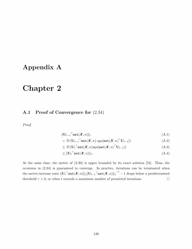
Appendix A
Chapter 2
A.1 Proof of Convergence for (2.34)
Proof.
‖Ut−1>mat(X , n)‖1 (A.1)
= Tr(Ut−1>mat(X , n) sgn(mat(X , n)>Ut−1)) (A.2)
≤ Tr(Ut>mat(X , n)sgn(mat(X , n)>Ut−1)) (A.3)
≤ ‖Ut>mat(X , n)‖1. (A.4)
At the same time, the metric of (2.30) is upper bounded by its exact solution [54]. Thus, the
recursion in (2.34) is guaranteed to converge. In practice, iterations can be terminated when
the metric-increase ratio ‖Ut>mat(X , n)‖1‖Ut−1
>mat(X , n)‖1−1 − 1 drops below a predetermined
threshold τ > 0, or when t exceeds a maximum number of permitted iterations.
139
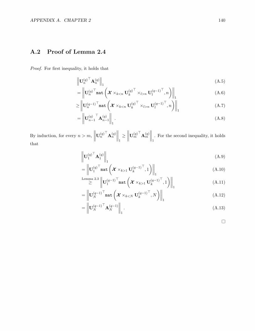
APPENDIX A. CHAPTER 2 140
A.2 Proof of Lemma 2.4
Proof. For first inequality, it holds that∥∥∥U(q)n
>A(q)n
∥∥∥1
(A.5)
=
∥∥∥∥U(q)n
>mat
(X ×k<n U
(q)k
>×l>n U
(q−1)l
>, n
)∥∥∥∥1
(A.6)
≥∥∥∥∥U(q−1)
n
>mat
(X ×k<n U
(q)k
>×l>n U
(q−1)l
>, n
)∥∥∥∥1
(A.7)
=
∥∥∥∥U(q)n−1
>A
(q)n−1
∥∥∥∥1
. (A.8)
By induction, for every n > m,
∥∥∥∥U(q)n
>A
(q)n
∥∥∥∥1
≥∥∥∥∥U(q)
m
>A
(q)m
∥∥∥∥1
. For the second inequality, it holds
that ∥∥∥∥U(q)1
>A
(q)1
∥∥∥∥1
(A.9)
=
∥∥∥∥U(q)1
>mat
(X ×k>1 U
(q−1)k
>, 1
)∥∥∥∥1
(A.10)
Lemma 2.3≥
∥∥∥∥U(q−1)1
>mat
(X ×k>1 U
(q−1)k
>, 1
)∥∥∥∥1
(A.11)
=
∥∥∥∥U(q−1)N
>mat
(X ×k<N U
(q−1)k
>, N
)∥∥∥∥1
(A.12)
=
∥∥∥∥U(q−1)N
>A
(q−1)N
∥∥∥∥1
. (A.13)

APPENDIX A. CHAPTER 2 141
A.3 Proof of Proposition 2.2
Proof. It holds that ∥∥∥U(q′)n
>A(q′)n
∥∥∥1
Lemma 2.4≥
∥∥∥∥U(q′)1
>A
(q′)1
∥∥∥∥1
(A.14)
Lemma 2.4≥
∥∥∥∥U(q′−1)N
>A
(q′−1)N
∥∥∥∥1
(A.15)
Lemma 2.4≥
∥∥∥∥U(q′−1)1
>A
(q′−1)1
∥∥∥∥1
(A.16)
≥∥∥∥∥U(q)
N
>A
(q)N
∥∥∥∥1
(A.17)
≥∥∥∥U(q)
n
>A(q)n
∥∥∥1. (A.18)
A.4 Proof of Lemma 2.5
Proof. Define x4= vec(mat (X , 1)) ∈ RP and Z
4= UN ⊗UN−1 ⊗ . . .⊗U1 ∈ SP×p. Then,
‖X ×n∈[N ] U>n ‖1 = ‖Z>x‖1 (A.19)
≤ √p‖Z>x‖2 (A.20)
≤ √p‖x‖2 =√p‖X‖F . (A.21)

Appendix B
Chapter 3
B.1 Proof of Lemma 3.1
Proof. Let Qopt be the solution to (3.1). Without loss of generality, there exists A ∈ Rρ×K and
B ∈ RD−ρ×K such that
Qopt = UA + UcB, (B.1)
where Uc ∈ RD×D−ρ is such that Uc>Uc = ID−ρ, span(U) ∩ span(Uc) = ∅, and dim(U) +
dim(Uc) = D. We notice that
X>Qopt = VΣU>UA + VΣU>UcB (B.2)
= VΣU>UA (B.3)
= X>UA. (B.4)
It follows that Qopt = UA for some A ∈ Rρ×K . Then, we define Y = ΣV> and observe that, for
any S ∈ Rρ×K , it holds
Y>S = VΣS (B.5)
= VΣU>US (B.6)
= X>US. (B.7)
By (B.4) and (B.7), if Aopt solves max.A∈Sρ×K ‖Y>A‖pp then Qopt = UAopt solves (3.1).
142

APPENDIX B. CHAPTER 3 143
B.2 Proof of Lemma 3.2
Proof. Let qopt ∈ RD solve max.q∈BD×1‖X>q‖pp. Assume that ‖qopt‖2 < 1 and consider the unit-
norm vector qopt = qopt‖qopt‖−2 1 ∈ BD×1. It holds that
‖X>qopt‖pp = ‖qopt‖−p2 ‖X>qopt‖pp > ‖X>qopt‖pp, (B.8)
which contradicts the assumption that ‖qopt‖2 < 1. Then, qopt solves max.q∈BD×1‖X>q‖pp and it
must be such that ‖qopt‖2 = 1. The latter implies that maxq∈SD×1‖X>q‖pp = maxq∈BD×1
‖X>q‖pp.
B.3 Proof of Lemma 3.3
Proof. Consider b,b′ ∈ ±1N such that b 6= b′. Assume that there exist q ∈ C(b) and q′ ∈ C(b′)such that q = q′. The latter implies that sgn(X>q) = sgn(X>q′) which can not be true since
sgn(X>q) = b 6= b′ = sgn(X>q′). We conclude that there is no q ∈ C(b) and q′ ∈ C(b′) such that
q = q′. Formally, C(b) ∩ C(b′) = ∅ for any b 6= b′.
B.4 Proof of Lemma 3.5
Proof. Consider b ∈ ±1N such that C(b) 6= ∅. Let q,q′ ∈ C(b) –i.e., sgn(X>q) = sgn(X>q′) =
b, ‖q‖2 ≤ 1, and ‖q′‖2 ≤ 1. First, notice that there exists a ∈ RN such that [a]n > 0∀n ∈ [N ] and
aX>q = X>q′. (B.9)
Consider θ ∈ [0, 1] and let q = θq + (1− θ)q′. It holds that
sgn(X>q) = sgn(θX>q + (1− θ)X>q′) (B.10)
= sgn(θX>q + (1− θ)aX>q) (B.11)
= sgn(X>q (θ1N + (1− θ)a)
)(B.12)
= sgn(X>q) (B.13)
= b. (B.14)
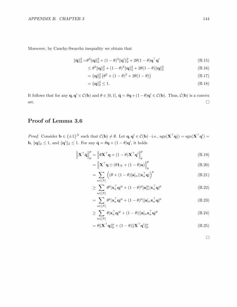
APPENDIX B. CHAPTER 3 144
Moreover, by Cauchy-Swarchz inequality we obtain that
‖q‖22 =θ2‖q‖22 + (1− θ)2‖q′‖22 + 2θ(1− θ)q>q′ (B.15)
≤ θ2‖q‖22 + (1− θ)2‖q‖22 + 2θ(1− θ)‖q‖22 (B.16)
= ‖q‖22(θ2 + (1− θ)2 + 2θ(1− θ)
)(B.17)
= ‖q‖22 ≤ 1. (B.18)
It follows that for any q,q′ ∈ C(b) and θ ∈ [0, 1], q = θq+ (1− θ)q′ ∈ C(b). Thus, C(b) is a convex
set.
Proof of Lemma 3.6
Proof. Consider b ∈ ±1N such that C(b) 6= ∅. Let q,q′ ∈ C(b) –i.e., sgn(X>q)) = sgn(X>q′) =
b, ‖q‖2 ≤ 1, and ‖q′‖2 ≤ 1. For any q = θq + (1− θ)q′, it holds∥∥∥X>q∥∥∥pp
=∥∥∥θX>q + (1− θ)X>q′
∥∥∥pp
(B.19)
=∥∥∥X>q (θ1N + (1− θ)a)
∥∥∥pp
(B.20)
=∑n∈[N ]
((θ + (1− θ)[a]n)|x>nq|
)p(B.21)
≥∑n∈[N ]
θp|x>nq|p + (1− θ)p[a]pn|x>nq|p (B.22)
=∑n∈[N ]
θp|x>nq|p + (1− θ)p|[a]nx>nq|p (B.23)
≥∑n∈[N ]
θ|x>nq|p + (1− θ)|[a]nx>nq|p (B.24)
= θ‖X>q‖pp + (1− θ)‖X>q′‖pp. (B.25)

APPENDIX B. CHAPTER 3 145
B.5 Proof of Lemma 3.7
Proof. Let qopt be the solution to (3.1). We find that
‖X>qopt‖pp =∑n∈[N ]
|x>nqopt|p (B.26)
=∑n∈[N ]
maxb∈±1
<(bx>nqopt)p. (B.27)
≥∑n∈[N ]
<
(bnx>nq)p
, (B.28)
where bn ∈ ±1∀n ∈ [N ]. Equality is attained if and only if bn = sgn(x>nqopt) for every n ∈[N ].
B.6 Proof of Proposition 3.2
Proof. Let B+D×1 = q ∈ RD : ‖q‖2 ≤ 1, [q]i ≥ 0∀i ∈ [D]. For any q ∈ BD×1, there exist a ∈ B+
D×1
and w ∈ ±1D, such that q = aw. Accordingly, it holds
maxq∈BD×1
‖X>q‖pp = maxq∈BD×1
∑n∈[N ]
|x>nq|p (B.29)
= maxa∈B+
D×1
maxw∈±1D
∑n∈[N ]
|(xn a)>w|p (B.30)
Lem. 3.6≤ max
a∈B+D×1
∑n∈[N ]
‖(xn a)‖p1 (B.31)
= maxa∈B+
D×1
∑n∈[N ]
|x>n a|p. (B.32)
The upper bound is attained by w = ±1D. Moreover, we notice that B+D×1 ⊆ C(1N ). Accordingly,
for non-negative X
maxq∈SD×1
‖X>q‖pp= maxq∈BD×1
‖X>q‖pp= maxq∈C(1N )
‖X>q‖pp. (B.33)

APPENDIX B. CHAPTER 3 146
B.7 Proof of Lemma 3.9
Proof. Consider B ∈ ±1N×K such that C(B) 6= ∅. Let Q,Q′ ∈ C(B) –i.e., sgn(X>Q) =
sgn(X>Q′) = B, ‖Q‖2 ≤ 1, and ‖Q′‖2 ≤ 1. First, notice that there exists A ∈ RN×K such
that [A]n,k > 0∀(n, k) ∈ [N ]× [K] and
AX>Q = X>Q′. (B.34)
Consider θ ∈ [0, 1] and let Q = θQ + (1− θ)Q′. It holds that
sgn(X>Q) = sgn(θX>Q + (1− θ)X>Q′) (B.35)
= sgn(θX>Q + (1− θ)AX>Q) (B.36)
= sgn(X>Q (θ1N×K + (1− θ)A)
)(B.37)
= sgn(X>Q) (B.38)
= Q. (B.39)
Moreover, the spectral norm satisfies the norm triangle inequality property. Therefore, it holds
‖Q‖2 =‖θQ + (1− θ)Q′‖2 (B.40)
≤ ‖θQ‖2 + ‖(1− θ)Q′‖2 (B.41)
= θ‖Q‖2 + (1− θ)‖Q′‖2 (B.42)
≤ θ + (1− θ) (B.43)
= 1. (B.44)
It follows that for any Q,Q′ ∈ C(Q) and θ ∈ [0, 1], Q = θQ + (1 − θ)Q′ ∈ C(B). Thus, C(B) is a
convex set.
B.8 Proof of Lemma 3.10
Proof. Assume that there exists k ∈ [K] such that b = [Bopt]:,k /∈ B?. Then, C(b) includes q = 0D
and [Qopt]:,k has no contribution in the metric. Substituting b by any b′ ∈ B? not in Bopt, would
offer a larger metric which contradicts that Qopt is the exact solution.

APPENDIX B. CHAPTER 3 147
B.9 Proof of Proposition 3.4
Proof. Let Qopt ∈ SD×K be the exact solution to (3.25). Consider Q′ ∈ SD×K and assume that
‖X>Qopt‖pp > ‖X>Q′‖pp. This contradicts that Qopt is the exact solution to (3.25). Accordingly,
there exists no matrix in Stiefel that offers a larger metric in (3.1) compared to Qopt.

Appendix C
Chapter 4
C.1 Proof of Lemma 4.1
Proof. Let bq4= y∗q ⊗ yq ∀q and define auxiliary variables v = 1L ⊗ sL, p = p⊗ 1L, v = sL ⊗ 1L,
and p = 1L ⊗ p.1 For any n ∈ 1 − L′, 2 − L′, . . . L′ − 1 and jn ∈ Jn, it holds that [bq]jn =
[y∗q ][v]jn[yq][v]jn
. Further, it holds
[yq][v]jn=
K∑k=1
v(θk)[p]jn ξq,k + [nq][v]jn
, (C.1)
[yq][v]jn=
K∑k=1
v(θk)[p]jn ξq,k + [nq][v]jn
. (C.2)
Next, we compute E[bq]jn =∑K
k=1 v(θk)ωjndk + σ2[iL]jn = [r]jn ,2 which implies that Er = r.
Then, for every n ∈ 1−L′, 2−L′, . . . , L′− 1 and (i, j) ∈ Jn , we define b(n)p,q,i,j
4= [b∗q ]i[bp]j . After
simple algebraic manipulations we find that
Eb(n)p,q,i,j
=∣∣gHn d + δ(n)σ2
∣∣2 + δ(q − p)∣∣ zHi,jd + δ(i− j)σ2
∣∣2 , (C.3)
1Recall that for any x ∈ N+, sx = [1, 2, . . . , x]>.2Recall that for any i ∈ 1, 2, . . . , L2, ωi = [p]i − [p]i.
148

APPENDIX C. CHAPTER 4 149
where gn4= [v(θ1)n, v(θ2)n, . . . , v(θK)n]>. Next, we proceed as follows.
e = E|[r]jn − [r]jn |
2
(C.4)
= |[r]jn |2 + E
[r]jn [r]∗jn
− 2E
<
[r]jn [r]∗jn
(C.5)
= E
[r]jn [r]∗jn− |[r]jn |
2 (C.6)
= E
1
Q2
Q∑q=1
Q∑p=1
[bq]jn [bp]∗jn
− |[r]jn |2 (C.7)
=1
Q2
Q∑q=1
Q∑p=1
Eb(n)q,p,jn,jn
− |[r]jn |
2 (C.8)
(C.3)=
(1>Kd + σ2)2
Q. (C.9)
C.2 Proof of Lemma 4.2
Proof. By Lemma 4.1, errr(rsel) = E‖rco − rsel‖22 =∑L′−1
n=1−L′ E|[r]jn − [r]jn |2 = (2L′ − 1)e.
C.3 Proof of Proposition 4.1
Proof. Notice that Z = F(IL′ ⊗ rco) = [F1rco, F2rco, . . . , FL′rco]. By definition, Fm is a selection
matrix that selects the L′−(m−1), L′−(m−2), . . . , 2L′−mth entries of the length-(2L′−1) vector
it multiplies, for every m ∈ 1, 2, . . . , L′. That is, Fmrco = [rco]L′−(m−1):2L′−m. Similarly, Zsel =
APPENDIX C. CHAPTER 4 150
[F1rsel, F2rsel, . . . , FL′ rsel] with Fmrsel = [rsel]L′−(m−1):2L′−m. In view of the above,
errZ(Zsel) = E∥∥∥Z− Zsel
∥∥∥2
F
(C.10)
= E
L′∑m=1
‖Fmrco − Fmrsel‖22
(C.11)
=L′∑m=1
E∥∥[rco]L′−(m−1):2L′−m − [rsel]L′−(m−1):2L′−m
∥∥2
2
(C.12)
=
L′∑m=1
L′−m∑n=1−m
E|[rco]L′+n − [rsel]L′+n|2
(C.13)
=L′∑m=1
L′−m∑n=1−m
e (C.14)
= L′2e. (C.15)
C.4 Proof of Lemma 4.3
Proof.
en = E
∣∣∣∣∣∣[r]jn −
1
|Jn|∑j∈Jn
[r]j
∣∣∣∣∣∣2 (C.16)
= |[r]jn |2 +
1
|Jn|2E
∣∣∣∣∣∣∑j∈Jn
[r]j
∣∣∣∣∣∣2− 2E
<[r]∗jn
1
|Jn|∑j∈Jn
[r]j
(C.17)
= |[r]jn |2 +
1
|Jn|2∑j∈Jn
∑i∈Jn
1
Q2
Q∑q=1
Q∑p=1
Eb(n)q,p,i,j
− 2<
[r]∗jn
1
|Jn|∑j∈Jn
[r]j
(C.18)
(C.3)=
1
Q
2σ21>Kd + σ4
|Jn|+∑i∈Jn
∑j∈Jn
|zHi,jd|2
|Jn|2
. (C.19)

APPENDIX C. CHAPTER 4 151
C.5 Proof of Lemma 4.4
Proof. By Lemma 4.3, errr(ravg) = E‖rco − ravg‖22 =∑L′−1
n=1−L′ E|[r]jn − 1|Jn|
∑j∈Jn [r]j |2 =∑L′−1
n=1−L′ en.
C.6 Proof of Proposition 4.2
Proof. We know that Z = [F1rco, F2rco, . . . FL′rco]. Thus, Zavg = [F1ravg, F2ravg, . . . FL′ ravg].
By the definition of Fm, for every m ∈ 1, 2, . . . , L′ it holds that Fmrco = [rco]L′−(m−1):2L′−m and
Fmravg = [ravg]L′−(m−1):2L′−m. In view of the above,
errZ(Zavg) = E∥∥∥Z− Zavg
∥∥∥2
F
(C.20)
= E
L′∑m=1
‖Fmrco − Fmravg‖22
(C.21)
=L′∑m=1
E∥∥[rco]L′−(m−1):2L′−m − [ravg]L′−(m−1):2L′−m
∥∥2
2
(C.22)
=
L′∑m=1
L′−m∑n=1−m
E|[rco]L′+n − [ravg]L′+n|2
(C.23)
=L′∑m=1
L′−m∑n=1−m
en. (C.24)
C.7 Proof of Lemma 4.5
We recall that w = 1Q
∑Qq=1 x∗q ⊗ xq. Next, we notice that by utilizing the auxiliary variables3
u = 1K+L⊗ sK+L and u = sK+L⊗1K+L, we obtain [w]i = 1Q
∑Qq=1[x∗q ][u]i [xq][u]i . Then, we define
I 4= i ∈ 1, 2, . . . , (K + L)2 : [i]i = 1. We observe that E[x∗q ][u]i [xq][u]i = δ([u]i − [u]i) = 1 if
3Recall that for any x ∈ N+, sx = [1, 2, . . . , x]>.
APPENDIX C. CHAPTER 4 152
i ∈ I and 0 if i /∈ I. The latter implies
Ew = i. (C.25)
Next, for (i,m) ∈ 1, 2, . . . , (K + L)22, we define
ηi,m4= [x∗q ][u]i [xq][u]i [x
∗p][u]m [xp][u]m . (C.26)
It holds [w]i[w∗]m = 1
Q2
∑Qq=1
∑Qp=1 ηi,m. By the 2nd and 4th order moments of zero-mean inde-
pendent normal variables, we find that Eηi,m is equal to 1 + δ(p− q)δ(i−m) if (i,m) ∈ I and 0
otherwise. The latter implies that E[w]i[w∗]m = 1
Q2
∑Qq=1
∑Qp=1 Eηi,m is equal to 1+ 1
Qδ(i,m),
if (i,m) ∈ I and 0 otherwise. Altogether, we have
EwwwH = ii> +1
QIK+L. (C.27)
C.8 Proof of Lemma 4.6.
Proof. For (i,m) ∈ 1, 2, . . . , L22, [H]i,m = [Vw]i[(Vi)∗]m =∑(K+L)2
j=1,l=1[V]i,j [w]j [V∗]m,l[i]l. Ac-
cordingly, [HE]i,m =∑(K+L)2
j=1,l=1 EΘEw[V]i,j [w]j [V]∗m,l[i]l. Considering that the random variables
w and V are statistically independent from each other and that Eww = i (see Lemma 4.5), we
obtain [HE]i,m = EΘ[Vi]i[(Vi)∗]m = EΘ[r]i[r∗]m. Then, we substitute4
[r]i =
K∑k=1
v(θk)ωidk + σ2[iL]i (C.28)
in EΘ[r]i[r∗]m. After plain algebraic operations, we obtain
[HE]i,m = ‖d‖22 I (ωi − ωm) + σ4δ(ωi)δ(ωm) + σ2(1>Kd
)(δ(ωi)I(−ωm) + I(ωi)δ(ωm)) (C.29)
+ I(ωi)I(−ωm)(
(1>Kd)2 − ‖d‖22). (C.30)
4Recall that for any i ∈ 1, 2, . . . , L2, ωi = [p]i − [p]i.

APPENDIX C. CHAPTER 4 153
C.9 Proof of Lemma 4.7.
Proof. For (i,m) ∈ 1, 2, . . . , L22 it holds
[G]i,m = [Vw]i[(Vw)∗]m =
(K+L)2∑j=1,l=1
[V]i,j [w]j [V∗]m,l[w
∗]l. (C.31)
Accordingly, [GE]i,m =∑(K+L)2
j=1,l=1 EΘEw[V]i,j [w]j [V∗]m,l[w
∗]l. Next, we recall that the random
variables Θ and w are statistically independent from each other. Thus,
[GE]i,m =
(K+L)2∑j=1,l=1
EΘ[V]i,jE
w[w]j [w
∗]l[V∗]m,l. (C.32)
The latter is equivalent to GE = EΘVE
wwwHVH. By Lemma 4.5, we obtain GE = E
ΘVii>VH+
1QVVH. By Lemma 4.6, we find that GE = HE + 1
QVE.
C.10 Proof of Remark 4.3
Proof.
‖T‖2F =D−1∑i=1−D
‖di(T)‖22 (C.33)
=
D−1∑i=1−D
‖ 1
D − |i|(1>D−|i|di(X))1D−|i|‖22 (C.34)
=
D−1∑i=1−D
(1>D−|i|di(X))2
(D − |i|)2‖1D−|i|‖22 (C.35)
=
D−1∑i=1−D
(1>D−|i|di(X))2
D − |i|(C.36)
≤D−1∑i=1−D
‖1D−|i|‖22‖di(X)‖22D − |i|
(C.37)
= ‖X‖2F . (C.38)
APPENDIX C. CHAPTER 4 154
C.11 Proof of Remark 4.5
Proof. Consider Hermitian T ∈ CD×D with EVD T = Udiag(λT )UH , U is unitary (i.e., UUH =
UHU = ID). Let H = UHP0U which implies that P0 = UHUH . It holds
minP0∈SD+
‖T−P0‖2F = minH∈CD×D
‖diag(λT )−H‖2F (C.39)
= minH∈CD×D
∑i,ji 6=j
[H]2i,j+D∑i=1
([λT ]i−[H]i,i)2 (C.40)
≥∑i,ji 6=j
[H]2i,j+D∑i=1
([λT ]i−[H]i,i) (C.41)
≥∑
i∈1,2,...,D|[λT ]i<0
[λT ]2i . (C.42)
Similar to [215], the lower bound in (C.42) is attained by matrix H = diag(λP ) for λP such that
[λP ]i = max[λT ]i, 0.
C.12 Proof of Remark 4.7
Proof.
‖A‖2F =D∑i=1
[λA]2i (C.43)
=
D−ρ∑i=1
[λP ]2i + ρ(1
ρ
D∑j=D−ρ+1
[λP ]j)2 (C.44)
≤D−ρ∑i=1
[λP ]2i +D∑
j=D−ρ+1
[λP ]2j (C.45)
= ‖P‖2F . (C.46)