theory and applications of compressive sensing
TRANSCRIPT

Purdue UniversityPurdue e-Pubs
ECE Technical Reports Electrical and Computer Engineering
12-8-2010
Theory and Applications of Compressive SensingAtul DivekarElectrical and Computer Engineering, Purdue University, [email protected]
Okan [email protected]
Follow this and additional works at: http://docs.lib.purdue.edu/ecetrPart of the Signal Processing Commons
This document has been made available through Purdue e-Pubs, a service of the Purdue University Libraries. Please contact [email protected] foradditional information.
Divekar, Atul and Ersoy, Okan, "Theory and Applications of Compressive Sensing" (2010). ECE Technical Reports. Paper 402.http://docs.lib.purdue.edu/ecetr/402

Theory and Applications of Compressive Sensing
Atul Divekar
Okan Ersoy
TR-ECE-10-07
December 8, 2010
School of Electrical and Computer Engineering
1285 Electrical Engineering Building
Purdue University
West Lafayette, IN 47907-1285

iv
TABLE OF CONTENTS
LIST OF TABLES...........................................................................................................................................vi
LIST OF FIGURES.................................................................................... ....................................................vii
ABSTRACT.................................................................................................................... ................................ix
PUBLICATIONS.............................................................................................................................................x
1. INTRODUCTION ...................................................................................................................................... 1
1.1 Overview Of Compressive Sensing .................................................................................................. 3 1.2 The Incoherence Parameter ............................................................................................................... 4 1.3 Example Of Recovery Using l1 Minimization .................................................................................. 4
2. SUPERRESOLUTION .............................................................................................................................. 7
2.1 Superresolution by Compressive Sensing ......................................................................................... 9
3. IMAGE FUSION ..................................................................................................................................... 12
3.1 Conventional Methods for Image Fusion ........................................................................................ 13 3.1.1 The IHS transform ................................................................................................................ 13 3.1.2 The Brovey transform ........................................................................................................... 13 3.1.3 Fusion by Principal Component Analysis ............................................................................ 14 3.1.4 Fusion by wavelet methods .................................................................................................. 14
3.2 Image Fusion by Compressive Sensing .......................................................................................... 15 3.2.1 Algorithm I ........................................................................................................................... 16 3.2.2 Algorithm II .......................................................................................................................... 17 3.2.3 A faster algorithm using the Karhunen-Loeve basis ............................................................. 19
3.3 A Modified Brovey Transform Algorithm ...................................................................................... 21 3.4 Comparison of Image Fusion Methods ........................................................................................... 22
3.4.1 Correlation Coefficient ......................................................................................................... 23 3.4.2 Spectral Angle Mapper ......................................................................................................... 23 3.4.3 ERGAS ................................................................................................................................. 24
4. CONTENT BASED IMAGE RETRIEVAL ............................................................................................ 32
4.1 Content Based Retrieval Architecture ............................................................................................. 34 4.1.1 Choice of metric ................................................................................................................... 35 4.1.2 Choice of sparsifying basis ................................................................................................... 35 4.1.3 Generating a query feature vector ......................................................................................... 36
4.2 Experimental Results ...................................................................................................................... 38

v
5. RECOVERY BY MULTIPLE PARTIAL INVERSIONS ....................................................................... 43
5.1 Improved Estimator by Multiple Partial Inversions ........................................................................ 43 5.2 Improved Orthogonal Matching Pursuit Algorithm Using Multiple Partial Inversions .................. 47 5.3 Use as a Direct Estimator ................................................................................................................ 48 5.4 Computational Complexity ............................................................................................................. 50 5.5 Experimental Results ...................................................................................................................... 51 5.6 Equation for Noise .......................................................................................................................... 55 5.7 Improvement in CoSaMP algorithm using the modified estimator ................................................. 58
6. SUMMARY ............................................................................................................................................. 62
LIST OF REFERENCES .............................................................................................................................. 63
VITA...............................................................................................................................................................66
vi
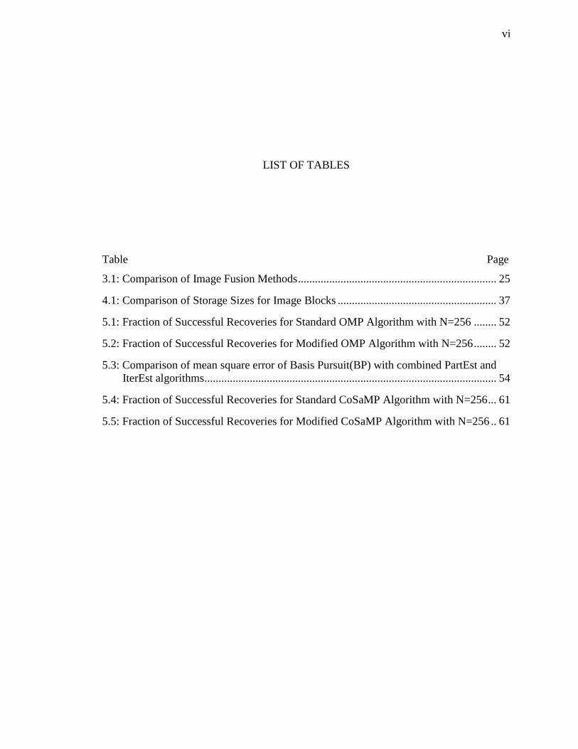
LIST OF TABLES
Table Page
3.1: Comparison of Image Fusion Methods ...................................................................... 25
4.1: Comparison of Storage Sizes for Image Blocks ........................................................ 37
5.1: Fraction of Successful Recoveries for Standard OMP Algorithm with N=256 ........ 52
5.2: Fraction of Successful Recoveries for Modified OMP Algorithm with N=256 ........ 52
5.3: Comparison of mean square error of Basis Pursuit(BP) with combined PartEst and
IterEst algorithms ....................................................................................................... 54
5.4: Fraction of Successful Recoveries for Standard CoSaMP Algorithm with N=256 ... 61
5.5: Fraction of Successful Recoveries for Modified CoSaMP Algorithm with N=256 .. 61

vii
LIST OF FIGURES
Figure Page
1.1: Left: Original image size 512x512; Right: Reconstructed image using 10000 largest
magnitude coefficients ................................................................................................. 2
1.2: Original signal with 40 nonzero entries on left, recovered signal on the right ............ 5
1.3: Orthogonal Matching Pursuit....................................................................................... 5
2.1: Superresolution by Regularization: Top Left: Original image; Top Right, Bottom
Left: Blurred images with subpixel shift; Bottom Right: Reconstructed image ......... 8
2.2: Superresolution by Compressive Sensing: Top Left: Original image, Top Right:
Blurred image, Bottom: Reconstructed image ........................................................... 11
3.1: Original LANDSAT Images: Top Left: Panchromatic image, resolution 15m; Top
Right, Middle Left, Right: Multispectral images in bands 2,3,4, resolution 30m;
Bottom: Combined multispectral images
................................................................................................................................... 26
3.2: Result of fusion by standard Principal Component Analysis Algorithm................... 27
3.3: Result of fusion by Algorithm I ................................................................................ 28
3.4: Result of fusion by Algorithm II (Segmentation) ...................................................... 29
3.5: Result of fusion by standard Brovey transform ......................................................... 30
3.6: Result of fusion by modified Brovey transform ........................................................ 31
4.1: Content Based Retrieval by compressed sensing ...................................................... 34
4.2: Original LANDSAT spectral band images ................................................................ 40
4.3 LANDSAT spectral band images reconstructed by l1 minimization .......................... 41
4.4: Reconstruction error in LANDSAT spectral band images ........................................ 42
4.5: Retrieval of single spectral band image from AVIRIS sensor: Left: Original image,
Middle: Reconstruction, Right: Reconstruction Error ............................................... 42

viii
Figure Page
5.1: Multiple Partial Inversions Algorithm PartEst .......................................................... 44
5.2: Example of Improved Estimation(Top to Bottom): Original Signal c with 60 nonzero
entries; Noisy estimate Tz y ; Noise z-c, sample variance 28.8, Improved
Estimator; Noise in improved estimator, sample variance 9.1 ................................. 46
5.3: Modified Orthogonal Matching Pursuit using Multiple Inversions........................... 47
5.4: Iterative Algorithm for Improved Estimator .............................................................. 48
5.5: Singular value distributions for matrices B and B1024
with Φ a 200 x 256 matrix
drawn from the Uniform Spherical Ensemble, W=160, A=50 ................................. 51
5.6: Signal used for comparison of Basis Pursuit with proposed algorithms ................... 53
5.7: Bias in noise terms: Cumulative sum for ,(1)L
j i for a 200*256 matrix Φ from the
USE with 800 Lj,i subsets randomly selected. ........................................................... 57
5.8: CoSaMP algorithm .................................................................................................... 59
5.9: Modified CoSaMP algorithm..................................................................................... 60

ix
ABSTRACT
Divekar, Atul, Ph.D. Purdue University, December 2010. Theory and Applications of
Compressive Sensing Major Professor: Okan Ersoy
This thesis develops algorithms and applications for compressive sensing, a topic in
signal processing that allows reconstruction of a signal from a limited number of linear
combinations of the signal. New algorithms are described for common remote sensing
problems including superresolution and fusion of images. The algorithms show superior
results in comparison with conventional methods. We describe a method that uses
compressive sensing to reduce the size of image databases used for content based image
retrieval. The thesis also describes an improved estimator that enhances the performance
of Matching Pursuit type algorithms, several variants of which have been developed for
compressive sensing recovery.
.

x
PUBLICATIONS
1) “Image Fusion by Compressive Sensing”, Proc. 17th
International Conference on
Geoinformatics, 2009
2) “Compact Storage of Correlated Data for Content Based Retrieval”, Proc. Asilomar
Conference on Signals, Systems and Computers, 2009.

1
1. INTRODUCTION
This thesis develops algorithms and applications in an emerging topic of signal
processing called compressive sensing. Compressive sensing developed from questions
raised about the efficiency of the conventional signal processing pipeline for
compression, coding and recovery of natural signals, including audio, still images and
video. The usual sequence of steps involved includes the following. First, the analog
signal is sampled by a sensor such as a camera to obtain a sufficiently large number of
digital samples. Second, the digitized samples are transformed into a suitable domain to
compact the energy (and hence the information) into a relatively small number of
numbers, called coefficients. The transformation is chosen to approximate the optimal
Karhunen-Loeve transform and results in a representation of the original signal as a linear
sum of a set of bases weighed by the coefficients. Most of the coefficients are small in
magnitude and only a few coefficients contain a significant amount of energy. This
implies that most of the information in the signal is concentrated in only a few bases of
the signal. Third, this sparsity of transform coefficients is exploited to efficiently code the
locations of the few large coefficients, and the magnitudes of these large coefficients are
quantized and entropy coded. Finally, the coded representation is stored and/or
transmitted to a decoder, where the coding and transformation steps are reversed to obtain
a good approximation of the original set of digital samples, which can be used for D/A
conversion and presentation to a viewer, with a quality close to that of the original
sampled scene.
2
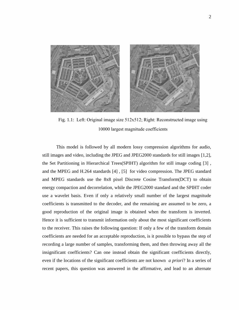
This model is followed by all modern lossy compression algorithms for audio,
still images and video, including the JPEG and JPEG2000 standards for still images [1,2],
the Set Partitioning in Hierarchical Trees(SPIHT) algorithm for still image coding [3] ,
and the MPEG and H.264 standards [4] , [5] for video compression. The JPEG standard
and MPEG standards use the 8x8 pixel Discrete Cosine Transform(DCT) to obtain
energy compaction and decorrelation, while the JPEG2000 standard and the SPIHT coder
use a wavelet basis. Even if only a relatively small number of the largest magnitude
coefficients is transmitted to the decoder, and the remaining are assumed to be zero, a
good reproduction of the original image is obtained when the transform is inverted.
Hence it is sufficient to transmit information only about the most significant coefficients
to the receiver. This raises the following question: If only a few of the transform domain
coefficients are needed for an acceptable reproduction, is it possible to bypass the step of
recording a large number of samples, transforming them, and then throwing away all the
insignificant coefficients? Can one instead obtain the significant coefficients directly,
even if the locations of the significant coefficients are not known a priori? In a series of
recent papers, this question was answered in the affirmative, and lead to an alternate
Fig. 1.1: Left: Original image size 512x512; Right: Reconstructed image using
10000 largest magnitude coefficients

3
model of sampling and signal recovery, called compressive sensing. We present an
overview of the basic principles of compressive sensing.
1.1 Overview Of Compressive Sensing
Consider an underdetermined system Φ where Φ with , is a
N-dimensional signal and is a length vector of measurements equal to linear
combinations of c . Suppose that has nonzero elements, and we wish to recover
from . One possible technique is to consider every subset Φ of columns drawn
from Φ and test whether it fits by least squares leaving no residue. However this
requires testing of subsets, which is infeasible for even moderate values of and
.
Recent papers [6,7] show that if has nonzero elements with
and the
matrix Φ satisfies some additional conditions, then can be recovered either exactly or
with a small approximation error. For example, it is shown in [7] that if matrix Φ satisfies
a Restricted Isometry Property(RIP), then minimization can recover the vector .
Explicitly, the matrix Φ satisfies the RIP with parameters for if
(1.1)
for every size subset of columns of Φ . If Φ satisfies the RIP with and
, then can be recovered perfectly by solving
If is not exactly sparse, but the components decay rapidly in magnitude, then can be
approximately recovered with a distortion that is bounded by
(1.3)
1min || || such that c y c
2 2 2
2 2 2(1 ) || || ||Φ || (1 ) || ||Ic c c
* 02 1|| || || ||S
Cc c c c
S
(1.2)

4
where is a small constant. The linear program in Equation (1.2) is a convex
optimization problem that can be solved efficiently by interior point methods. However it
is difficult to prove that a matrix Φ satisfies the RIP, and for large signals the convex
optimization can still be computationally slow.
1.2 The Incoherence Parameter
An alternative formulation to Restricted Isometry has been defined in [8] that lower
bounds the number of samples needed for perfect recovery using an incoherence
parameter µ. Suppose that V (size n x n) is an orthogonal matrix satisfying VTV=nI and
,max | |ij
i jV . Select any M rows from V, to give the M x N matrix Φ as before. If the
signal c has m nonzero values that are ±1, and if 2
0 log( / )M C m n and also
2
1 log ( / )M C n for some constants C0 and C1, then with probability exceeding 1-δ, the
signal c can be recovered by solving the same l1- minimization mentioned above.
1.3 Example Of Recovery Using l1 Minimization
We illustrate the results above with some examples. The RIP property is satisfied
with high probability for Gaussian matrices, i.e., matrices with entries drawn from a
Gaussian distribution [7]. We construct a size 128 x 200 matrix U with entries drawn
from a 0-mean Gaussian distribution with variance 1/128. This makes 2
2[|| || ] 1iE U for
all i, where Ui denotes the ith
column of U.
We form a sparse vector c with 40 nonzero entries drawn from a random distribution.
This is used to get y Ux , a length 128 sized sample vector. We then use l1-minimization
as described above to recover the signal x. We show the original signal and the recovered
signal in Fig. 1.2.

5
A second approach to this problem involves greedy algorithms such as
Orthogonal Matching Pursuit (OMP) [9] and its variants [10] [11] [12] [13]. In these
algorithms, the projection Φ of the data is used to identify a single or a few bases
that is/are believed to be in the true signal, and then the component of the data that is
spanned by all the bases selected so far is removed, leaving behind a residue that is
orthogonal to the bases selected. The residue is then used to identify more bases using
Tz r . The Orthogonal Matching Pursuit algorithm is listed in Fig. 1.3.
Fig. 1.2: Original signal with 40 nonzero entries on left, recovered signal on the right
Fig. 1.3: Orthogonal Matching Pursuit

6
In [9] it is shown that if is S-sparse and Φ is known with Φ a
sampling matrix consisting of zero mean normal random variables with equal variances,
OMP recovers in iterations if ,where is a constant. Failure
cases are discussed in [14]. The CoSaMP algorithm [10] provides error bounds
equivalent to l1 minimization and the speed of the OMP algorithm provided that the RIP
constant . This implies a relatively small range of eigenvalues (
) allowed for each column subset of Φ, and verifying that Φ satisfies the
RIP is also computationally difficult. In general, deterministic Matching Pursuit(MP)
algorithms suffer from an important weakness: it is possible to construct signals Φ
for which the MP algorithm makes a wrong choice for a basis believed to be in the
original signal, removes this basis from the samples, and then is led astray in making
future choices.
The literature also contains compressive sensing recovery applications where the
recovery works very well, even though the Φ matrix contains highly correlated columns
which do not satisfy any reasonable bound on the RIP constants for even small values of
. An example is the face recognition work in [15] where a dictionary contains highly
similar faces and recognition is successfully carried out by minimization. In this work
the class of faces that contains most of the resultant weights, is returned as the identifying
solution. Indeed, Restricted Isometry is a sufficient, but not necessary, condition for
compressive sensing recovery.
In this work, we aim to (i) exploit compressive sensing to develop novel algorithms
for problems in remote sensing and (ii) contribute to the theory of compressive sensing
by developing recovery algorithms that are superior to existing work and provide a
different understanding of the topic.

7
2. SUPERRESOLUTION
Superresolution is a common image processing operation that attempts to increase
the resolution of an image given one or more low resolution images and/or a prior model.
The desired high resolution image is related to the available image(s) by a forward model
that is represented as a matrix Φ. The matrix typically contains coefficients of a low pass
filter. Let x be the vectorized N x N high resolution image to be reconstructed and y be
the low-resolution N/2 x N/2 image or images. Then we relate the low resolution and
high resolution images by y x . We may try to obtain the solution by solving
(2.1)
However, the solution to this problem is unstable and can vary wildly due to small
changes in the data, or noise. This occurs because the matrix Φ has very small singular
values. The problem is said to be ill-posed because the solution does not vary in a smooth
and continuous way with the data. A common solution [16] is to regularize the problem
by adding a constraint that reflects a priori knowledge about the domain of image x. This
converts the problem into a well-posed problem with a unique and stable solution.
Commonly, the smoothness of the image –a property of most natural images- is used as a
constraint. For example, we modify the solution to
Here D is a high pass filter such as the Laplacian kernel matrix. The second term
penalizes the differences between neighboring pixels, and λ is the Lagrange multiplier
that determines the relative significance of the first and second terms. An example of
2 2
2 2x̂= argmin ||y- x|| || ||x Dx
2
2x̂= argmin ||y- x||x
(2.2)

8
superresolution by regularization using the Laplacian kernel and two blurred images with
subpixel offsets is shown in Fig. 2.1.
Fig. 2.1: Superresolution by Regularization: Top Left: Original image; Top Right,
Bottom Left: Blurred images with subpixel shift; Bottom Right: Reconstructed image

9
2.1 Superresolution by Compressive Sensing
We suggest an alternative method of superresolution based on compressive sensing.
This algorithm uses a dictionary DH of 4x4 pixel patches taken from high resolution
training images that have the same statistical properties as the image to be reconstructed.
Each patch has its mean subtracted out. For each patch in DH we produce a low-
resolution “sample” patch by blurring with the same operator Φ used in the forward
model. The dictionary DL of low-resolution patches is used for l1 minimization to
reconstruct each 4x4 high resolution patch. To ensure continuity of features in the
reconstructed image, we use overlapped patches with the left and upper 1-pixel strips of
the current patch taken from the already reconstructed left and upper neighbor patches.
This provides 7 more “samples” to add to DL. Thus the basic algorithm is
From the training images
1) Obtain a 4x4 size patch dictionary DH (size 16*K, where K is the number of
samples).
2) For each patch in DH construct a sample vector that has four 2x2 pixel means and
the same 7 samples as the left and top 1-pixel strips of the high resolution patch.
This gives the low resolution sample dictionary DL. This has size 11*K. Find the
means mDH and mDL of DH and DL respectively. Set (:, ) (:, )H H HD k D k mD
and (:, ) (:, )L L LD k D k mD for each column k.
3) Normalize each column of DL to have unit norm. Store the norms in vector n.
To reconstruct the high resolution image:
For each 4x4 patch in raster order and 1 pixel overlap with previously reconstructed
patches,
1) Use low resolution pixels (2x2) and samples from left and upper reconstructed
patches to construct length 11 vector y. (For the top and leftmost rows of patches, we
use an estimate of the top and/or left pixel edges using a standard method such as
Brovey). Set Ly y mD .

10
2) Solve 1
L
min ||a||
such that y=D a
3) Normalize . /a a n . The estimate for the high resolution patch is ˆH Hx D a mD .
The performance of this algorithm depends on the similarity of the patches in
the dictionary to the actual patterns present. (If the exact pattern is present in the
dictionary it will always be recovered provided that every pair of columns of DL is
linearly independent). For the Landsat training images we used, about 10000 patches are
sufficient to recover high resolution image with sufficient visual quality.
Since each low resolution patch is obtained by a blurring operation, it is possible
for two high resolution patches to map to a single (or negligibly different) low resolution
vector. In this case the l1-minimization algorithm can pick the wrong signal as the high
resolution reconstruction. However, providing the top and left 1-pixel strips seems to be
sufficient to obtain good separation between otherwise similar low-resolution patches. If
the mean is subtracted from DL we get Gaussian statistics. In [7] it is proven that such a
Gaussian matrix almost always has the Restricted Isometry Property, and hence l1
minimization will recover the correct linear combination to reconstruct the high
resolution image.
To reduce the computational complexity, it is possible to use the Karhunen-
Loeve transform matrix V of size 16 by 16 corresponding to the dictionary DH in place of
the full dictionary. This is obtained by finding the covariance matrix of the columns of
DH-mDH followed by the Singular Value Decomposition. We obtain DL by multiplying
V by an 11*16 projection matrix P, which captures the means of the 2x2 blocks, and the
exact pixel values from the top and left strips. We used this technique in our
implementation.
An example of superresolution by compressive sensing is shown in Fig. 2.2.

11
Fig. 2.2: Superresolution by Compressive Sensing: Top Left: Original image, Top Right:
Blurred image, Bottom: Reconstructed image

12
3. IMAGE FUSION
Image fusion is a technique that combines images of a scene from different
sensors to discover knowledge that is not apparent from any single image alone. Image
fusion finds applications in analysis of satellite images, surveillance and security, and
medical imaging, where images from multiple modalities such as MRI, CT and PET may
be combined for better visualization and diagnosis.
Remote sensing satellites such as the LANDSAT series commonly include a high
resolution panchromatic camera, and a multispectral sensor with several bands and lower
spatial resolution in each band than the panchromatic camera. For example, the
LANDSAT-7 satellite has a panchromatic camera of 15m resolution and 7 multispectral
band sensors with resolution 30m. In this context, the goal of image fusion is to combine
the high resolution panchromatic image and the lower resolution multispectral images to
produce an image in each multispectral band which is as close as possible to what would
be produced by observing the same ground area by a multispectral sensor with the same
resolution as the panchromatic camera. Thus the fused image should match the
panchromatic image in spatial resolution while preserving the spectral characteristics of
the low resolution multispectral images.
Common methods for fusion of remote sensed images include the IHS transform
[17], the Brovey transform [18], Principal Component Analysis(PCA) [19] and wavelet
based methods [20,21]. We briefly review these methods.

13
3.1 Conventional Methods for Image Fusion
3.1.1 The IHS transform
The IHS (Intensity-Hue-Saturation) transform first converts a RGB color image
into the IHS space which is correlated to human color perception. The low resolution
RGB image is first interpolated to the resolution of the panchromatic image. Then the
pixels at each spatial location i denoted Ri, Gi and Bi are transformed to the IHS space.
The transformation is given by
0
0
1
1/ 3 1/ 3 1/ 3
2 / 6 2 / 6 2 2 / 6
1/ 2 1/ 2 0
I R
v G
Bv
(3.1)
The low resolution intensity component in the IHS space I0 is replaced by the high
resolution panchromatic image Inew and the transformation is inverted to give
1
2
1 1/ 2 1/ 2
1 1/ 2 1/ 2
1 2 0
new
i new
new
i
new
i
R I
G v
vB
(3.2)
3.1.2 The Brovey transform
In this transform, the magnitude of the pixel from the panchromatic image is divided
in proportion to the relative strengths of the pixel magnitudes for each band. For a given
2x2 pixel block p from the panchromatic image, let ib be the value of the

14
corresponding single pixel in the low resolution image of band i . Then the standard
Brovey method gives the fusion result for this 2x2 block in band i by
(3.3)
3.1.3 Fusion by Principal Component Analysis
This technique utilizes a transformation of the original spectral images into the
Karhunen-Loeve basis that decorrelates the spectral bands. Let
i
i i
i
R
X G
B
be the pixel
vector at location i and let µ be the mean of Xi over all spatial locations i of the
multispectral images. Then the sample covariance matrix is given by1 T
i i
i
C X XN
.
The eigenvectors of the covariance matrix provide the optimal decorrelating basis for the
spectral bands, which is called the Karhunen-Loeve basis. Let the basis be represented by
a 3x3 matrix A. Then we obtain i iP AX , where Pi are the principal components at pixel
i. The first principal component PC0 contains the maximum energy among all the
components. This is replaced by the panchromatic image and the transform A is inverted
to give the fused image.
3.1.4 Fusion by wavelet methods
A wavelet transform carries out a subband decomposition of an image, separating
low frequency (smooth) and high frequency (edge-like) features. This allows the injection
of high resolution (sharp) features from the wavelet transform of the high resolution
panchromatic image into the wavelet transform of the low resolution multispectral
=1,2,3
=f ii
j
j
bb p
b

15
images. The multispectral image is interpolated and transformed to the wavelet domain.
The panchromatic image is also transformed to the wavelet domain. The high frequency
coefficients from the panchromatic image are merged (added) into the high frequency
subbands of the multispectral image, and then the transform is inverted to obtain the
fused image.
The critically sampled wavelet transform is shift-variant, and does not preserve
the edges in the fused image well. To overcome this problem an oversampled
decomposition known as the a trous wavelet transform [22] is used. This is a
nonorthogonal wavelet decomposition defined by a filter bank {hi} and {gi=δi-hi} where
δi denotes the Kronecker delta function, and represents the allpass operator. Instead of
decimation, the lowpass filter is upsampled by the appropriate power of 2. The detail
signal is given by the pixel difference between two successive approximations. The fused
images show better edge continuity features than with the critically sampled wavelet
transform [21].
3.2 Image Fusion by Compressive Sensing
We propose three new algorithms that utilize compressive sensing for image
fusion. Compressive sensing requires the system matrix to satisfy the RIP property. This
may be achieved in two ways : (i) by explicitly constructing a matrix to satisfy RIP, and
(ii) by reducing the problem to a matrix that is known to satisfy RIP, such as a Gaussian
matrix. We use the latter method. We first define a model for the expected high
resolution fused images given the data. This is used to generate a library of candidates for
the high resolution fused images. Corresponding to each candidate in the high resolution
library we generate a feature vector in another library. Let the library of candidate images
be HD , and the library of feature vectors be LD .
For the first method, we utilize the PCA fusion result as a starting point. Since the
PCA result has good spatial detail but suffers from spectral distortion, we modify the
spectral properties of the PCA result in a random manner while maintaining the spatial
features of the PCA results.

16
3.2.1 Algorithm I
We use the PCA algorithm to fuse the low resolution MS bands with the
panchromatic image. Let the fused images be 1b , 2b and 3b . We divide the fused images
into 16x16 pixel blocks. Let j
ib be the thj block of the thi band, and j
id be the 8x8 pixel
block in the original low resolution band i corresponding to this block.
For each 16x16 pixel block j
ib ,
1. For each 4x4 block of j
ib , subtract out the mean value.
2. Create HD and LD , matrices of size 256*S and 64*S respectively, where S
is the number of samples. For each sample in HD , add a random number drawn from
N(0,1) to the mean of each 2x2 block. LD contains the mean value of each 2x2 block
after adding the random number.
3. For each 2x2 block of j
id , subtract out the mean value. Call the resulting
length 64 vector y and the vector of means .
4. Let HmD be the mean of HD and LmD be the mean of LD . Subtract HmD
and LmD from each column of HD and LD , respectively.
5. Let n be a length S vector with 2=i Lin D . Normalize /Li Li iD D n .
6. Solve 1min || || such that =L Lc y mD D c
7. Normalize /i i ic c n .
8. Set ˆ j
i H Hx mD D c . Here ˆ j
ix is the fused result corresponding to the
thj block of the thi band and is the vector interpolated to match the dimensions of
ˆ j
ix .

17
Note that after LmD is subtracted out of LD , only the Gaussian residue is left
behind. LD is then normalized to have unit-norm columns. Such a Gaussian matrix is
known to satisfy RIP with overwhelming probability [7]. Also, the reconstructed block is
likely to be a sparse linear combination of the columns of HD . This justifies the use of
the results related to RIP to reconstruct the fused images.
We utilized the public-domain software package l1-magic to implement the l1
minimization algorithm. We found that about 8000 samples was sufficient to produce
acceptable results.
3.2.2 Algorithm II
For the second algorithm we segment the panchromatic image and randomly
modify the mean values of each region. To maintain spatial detail, we wish to preserve
the difference between each pair of adjacent segments.
For each K*K block at high resolution, let id be the low-resolution 2 2
K KX block
from low resolution MS band i .
1. Segment the K*K panchromatic image block to get C regions.
2. Find the adjacency matrix for the segmentation map.
3. To create HD and LD , matrices of size 2K *S and 2
4
K*S respectively,
where S is the number of samples:
Let v be the vectorized panchromatic image block with zero mean. For each
sample k ,

18
(a) For each pair of adjacent regions ( , )i j in the segmentation map, find a
random number r from (0,1)N . Add r to each pixel of region i in v , and r to each
pixel of region j in v .
(b) Set H kD v . Find the mean of each 2x2 pixel block in v to give LkD .
(c) Let HmD be the mean of HD and
LmD be the mean of LD . Subtract
HmD and LmD from each column of HD and
LD , respectively
(d) Let ( )imean d , and let iy d .
(e) Let n be a length S vector with 2=i Lin D . Normalize /Li Li iD D n .
(f) Solve 1min || || such that =L Lc y mD D c
(g) Normalize /i i ic c n .
(h) Set ˆH Hx mD D c . This is the fused result.
We improved the performance of this algorithm by segmenting a linear
combination of the panchromatic image and the interpolated MS image for each band.
Let dnp be a blurred version of the panchromatic image with size / 2* / 2K K . Let
< , >=
|| |||| ||
dn ii
dn i
p b
p b be the correlation coefficient. Let in
ib be the interpolated MS band
images. We use 2 2= (1 ) in
iz p b for the segmentation for each band i . The rationale
is that if the correlation is high, the panchromatic image contains valid information for
the band and should be weighed heavily, otherwise the low-resolution image should be
relied on.

19
3.2.3 A faster algorithm using the Karhunen-Loeve basis
In this algorithm, we utilize training samples from panchromatic and MS band
images to learn the statistics of the images we wish to generate. We use the Karhunen-
Loeve basis that optimally sparsify the sample vectors. Since the number of bases is
much smaller than the number of samples, 1l minimization takes much less time. We use
the result of the standard PCA algorithm to extract the desirable properties for the fusion
result. To avoid confusion, we refer to the standard PCA algorithm as sPCA. Since the
sPCA result shows color distortion, we use the low resolution MS band images to specify
the mean of each 2x2 block in the fusion result, and ensure that this information is not
obtained from the sPCA result. We assume that the image statistics over 8x8 windows are
almost invariant from the highest resolution to the next coarser resolution. This allows us
to train the algorithm with low resolution images and use them to synthesize high
resolution images.
1. Use the sPCA algorithm to fuse the low resolution MS bands with the
panchromatic image. Let the fused images be 1b , 2b and 3b .
2. Extract 8x8 pixel blocks from corresponding locations of the three MS
bands to generate a 8x8x3 length sample vector. Construct a library HD of size 192*K
with K samples of training data.
3. Let HmD be the mean of HD . Remove it from each sample of HD . Find the
covariance matrix =1
1=
K T
H i H iiC D D
K . Find its eigevector matrix V such that = TC VSV
4. Let ,i jb , 1<= <= <= 4i j , be a 8x8 matrix that has value 1
2 at the 2x2 block
bounded by 2 1,2i i and 2 1,2j j . Let B be the matrix of vectorized ,i jb for
1<= <= <= 4i j . Let W be the matrix defined as

20
0 0
0 0
0 0
B
B
B
Here 0 is a 64*48 matrix of 0s.
5. Define G , a 192*D size matrix with elements drawn from a 0-mean
Gaussian distribution with variance 1/192. We chose D=80.
6. Find = TP W G and =R G WP . Let = [ ]Z WR .
7. Define = T
LV Z V and = T
L HmD Z mD .
8. Let n be a length 192 vector with the norm of each column of LV .
Normalize each column to unit norm.
9. To fuse the thi 8x8 block,
(a) Concatenate block i of each of 1b , 2b and 3b to form vector iz .
(b) Let t be the vector of 4x4 pixel blocks from the MS band images
corresponding to block i .
(c) Define [2 ]T T T
iy t z R
(d) Solve 1min || || such that =L Lc y mD V c
(e) Normalize /i i ic c n .
(f) Set ˆH Hx mD D c . This is the fused result.
Here W is a matrix of basis vectors corresponding to 2x2 pixel block means from
each band. We define a set of random basis vectors G from a Gaussian distribution and
remove any components of these vectors in the subspace spanned by W to obtain R . The

21
result of the sPCA algorithm is projected onto vectors R , and these projections together
with the low resolution pixel values provide the data vector y . For each column in V , a
vector is generated in the same manner to obtain LV , which is used for 1l minimization.
3.3 A Modified Brovey Transform Algorithm
In Algorithm II and the KLT-based algorthm, we removed the distortion in the
sPCA result by modifying the low resolution spectral values. This leads us to propose a
modification for the standard Brovey transformation method for image fusion that greatly
reduces spectral distortion while maintaining the computational complexity of the
standard Brovey transform.
For a given 2x2 pixel block p from the panchromatic image, let ib be the value
of the corresponding single pixel in the low resolution image of band i . Then the
standard Brovey method gives the fusion result for this 2x2 block in band i as
We may write = dp p for the 2x2 panchromatic block, with the 2x2 block mean
and dp the residue after the mean is removed. Then we have
Since each pixel in f
ib is a multiple of the corresponding pixel in ib , the Spectral Angle
Mapper value remains 0. However the ratio
=1,2,3
d
jj
p
b
changes from each 2x2 block to
=1,2,3
=f ii
j
j
bb p
b (3.4)
=1,2,3
= ( )f ii d
j
j
bb p
b
(3.5)

22
the next,causing heavy spectral distortion. We propose a simple modification that reduces
the spectral distortion:
This reduces the variability in the ratio over the image while maintaining the
simplicity of the Brovey transform. we found that fine details were more easily
distinguishable in the fused result if a multiple , 1< < 2 , was used along with dp in
the equation. We chose =1.3 .
3.4 Comparison of Image Fusion Methods
We provide a comparison of our fusion results using three commonly used
measures: the Spectral Angle Mapper(SAM) value between the low-resolution MS image
and the fused image, the Correlation Coefficient between the panchromatic image and the
fused MS images, and the ERGAS measure [23], which is designed specifically to
measure fusion performance (a smaller value indicates better performance).
We first define the measures. Let p be the K x K panchromatic image,
1 2 3, ,d d db b b be the x 2 2
K K low resolution multispectral band images, 1 2 3, ,b b b be the
interpolated band images, and 1 2 3ˆ ˆ ˆ, ,b b b be the fused K x K images.
=1,2,3
= (1 )f di i
j
j
pb b
b
(3.6)

23
3.4.1 Correlation Coefficient
The Correlation coefficient for band i is defined as
Here () defines the mean of the respective image. Higher values of Correlation
Coefficient indicate better spatial fidelity with the panchromatic image.
3.4.2 Spectral Angle Mapper
Let
1
2
3
ˆ
ˆˆ =
ˆ
j
jj
j
b
v b
b
and
1
2
3
=
j
jj
j
b
v b
b
be the pixel vectors at location j in the fused
bands, and in the interpolated bands respectively. Then we define the Spectral Angle
Mapper(SAM) value as
It measures the average correlation between spectral vectors in the original and fused
band images. A low value indicates good spectral fidelity. This value is 0 if each ˆjv is a
scalar multiple of the corresponding jv . This happens with the standard Brovey
transform algorithm. However, this does not necessarily lead to good visual color fidelity
since the constant changes from one 2x2 block to the next.
ˆ
ˆ
ˆ( ) ( )=
ˆ|| |||| ||
T
p i bi
i
p i bi
p bCC
p b
(3.7)
2
2=1
ˆ< , >1= arccos
ˆ|| |||| ||
Kj j
j j j
v vSAM
K v v
(3.8)

24
3.4.3 ERGAS
ERGAS is a frequently used quality measure defined in [23]. It stands for erreur
relative globale adimensionnelle de synthese which means relative dimensionless global
error in synthesis. It measures properties that the synthetic (fused) image should try to
achieve:
1. Each high resolution image ˆib on being degraded (blurred) to low resolution
should be as identical as possible to the given low resolution image idb .
2. Each high resolution image ˆib should be as similar to the images that the
multispectral sensor would capture if it worked at the higher resolution.
3. The set of high resolution images 1 2 3ˆ ˆ ˆ, ,b b b should be as identical as possible
to the multispectral set of images that the corresponding sensor would observe with the
highest spatial resolution h .
ERGAS is defined as
Here iRMSE is the root mean square error between the fused and interpolated
low-resolution image of band i , i is the mean of the band i image and h
l is the ratio of
the size of low resolution to high resolution pixels. (It is 1
2 if each low resolution image
pixel is the mean of a 2x2 block of high resolution pixels). A low value of ERGAS
indicates good fidelity to the data.
We compare the results of our algorithms with those of the PCA and Brovey
transform methods.We see that all the compressive sensing algorithms have much better
spectral distortion performance (as measured by SAM and ERGAS) than the standard
2
2=1..3
1= 100 i
i i
RMSEhERGAS
l N (3.9)

25
Brovey and PCA methods. The modified Brovey transform shows much lower spectral
distortion than the standard method.
Table 3.1: Comparison of Image Fusion Methods
Method SAM
(deg) CC ERGAS
Standard Brovey 0 0.79 0.87 0.74 39.4
Principal
Components 9.59 0.91 0.93 0.77 21.43
Compressive
sensing-I 4.85 0.64 0.78 0.71 11.62
Compressive
sensing-SEG 5.6 0.68 0.77 0.93 13.5
Compressive
Sensing -KLT 6.3 0.80 0.88 0.9 11.5
Low Cost Brovey 0 0.48 0.60 0.79 4.84

26
Fig. 3.1: Original LANDSAT Images: Top Left: Panchromatic image, resolution 15m;
Top Right, Middle Left, Right: Multispectral images in bands 2,3,4, resolution 30m;
Bottom: Combined multispectral images

27
Fig. 3.2: Result of fusion by standard Principal Component Analysis Algorithm

28
Fig. 3.3: Result of fusion by Algorithm I

29
Fig. 3.4: Result of fusion by Algorithm II (Segmentation)

30
Fig. 3.5: Result of fusion by standard Brovey transform

31
Fig. 3.6: Result of fusion by modified Brovey transform
32
4. CONTENT BASED IMAGE RETRIEVAL
Satellite image databases store vast volumes of image data acquired from a
variety of satellite platforms.These include multispectral and hyperspectral sensors that
capture a 3D image cube for each spatial scene.For example, NASA's AVIRIS sensor can
produce a data cube of size 512*512 pixels and 224 bands with 16 bits per sample
giving a size of 112 MB for a single spatial scene. NOAA satellite image archives are
expected to grow from 300 TB in 2000 to 15000 TB in 2015, mainly due to hyperspectral
data. Manually annotating images in such large archives with information that can be
searched by a text based query is impractical.
Content Based Image Retrieval(CBIR) [24,25] is a technique for recovery of
images from an image database by specifying non-textual properties that the image is
expected to have. These properties are used to generate a query feature vector. Each
image in the database is associated with a similar feature vector. A suitable metric is used
to find the feature vector that best matches the query feature vector, and the
corresponding image is returned as the result of the query.
CBIR databases have been previously developed for remote sensing and medical
applications. The feature vectors in CANDID [26] contain histograms from gray levels
and in QBIC [27] [28] contain global characteristics such as color histograms, shape
parameters and texture values. In [28] spatio-spectral properties of multispectral images
are used for retrieval from databases of MS/HS images. A framework for information
mining in image databases is presented in [29] integrating spectral information from a
classifier and spatial information based on Gabor wavelet coefficients.
CBIR can provide search capabilities for MS/HS data that are not possible with
textual queries. For example, a geologist may look for a particular spectral signature

33
corresponding to a mineral that is embedded in a hyperspectral image with a specific
spatial pattern. The geologist may be presented with candidate spatial patterns and
mineral patterns and asked to select those desired.
We describe a method to reduce the storage needed for each image record that
utilizes compressive sensing and the information stored in the feature vector.
We use correlations (dot product values) of the images with spatial patterns as the
elements of our feature vectors. For an image x , the feature vector is obtained as =y x ,
where the rows of contain the spatial patterns.The spatial patterns may be obtained by
randomly sampling the database, from centroids obtained by clustering image patches, or
even by sampling random distributions. The first two kinds of spatial patterns provide an
intuitive characterization of the image being described: A high correlation value indicates
that the pattern closely matches the image content. The correlations can be obtained at
multiple scales, allowing for the possibility of searching for an image with coarse scale
global patterns and specific fine scale features in some locations. Feature vectors
obtained by correlation directly indicate the pattern content of the image, and are suitable
for reconstruction of the image by compressive sensing. They can also be augmented by
parameters such as color content and texture values utilized in previous work if desired.
The query feature vector can be generated by correlations of the spatial patterns
with a known exemplar image or estimated from a user's judgement of the match between
the pattern and the desired image. We consider both possibilities in the sequel.

34
4.1 Content Based Retrieval Architecture
Fig. 4.1: Content Based Retrieval by compressed sensing
The schematic for the CBIR system is shown in Figure (1). We assume that the
multispectral data has K bands. Each band is divided into *B B spatial blocks and each
cube of size = * *N K B B pixels is vectorized and stored as a record x . A query vector
is generated as described below.The Euclidean distance 2|| ||q y is used as a metric to
find the feature vector y in the database that is closest to the query feature vector q . The
vector y is used to obtain a reconstruction *x of the image x . The recovered signal *x
does not exactly match x because the original image is compressible, rather than exactly
S-sparse. We store the error *x x along with the feature vector y in the database. Since
*x x has far less energy than the original image, it requires very few bits for storage

35
compared to the original image. The magnitude of *x x is bounded as described in the
first chapter. We consider several topics related to the architecture below.
4.1.1 Choice of metric
If the matrix satisfies the Restricted Isometry Property, multiplying the length
N vectors ix by produces length M projections =i iy x that have the same
Euclidean distance relationships as the vectors ix . i.e. if 2 2
1 2 1 3|| || <|| ||x x x x , then
2 2
1 2 1 3|| || <|| ||y y y y . If has entries from a Gaussian distribution with unit norm
columns, the Johnson-Lindenstrauss lemma [30] indicates that the Euclidean norm is
preserved by the projection. In this case and also when the rows of are patterns
randomly taken from the image database, all the entries of the feature vector carry equal
importance, and we choose a simple Euclidean norm to identify the feature vector that is
closest to the query. Other norms such as the 1l metric are also possible, and this is a
topic for future research.
4.1.2 Choice of sparsifying basis
We considered different choices of sparsifying bases for this data. The optimal
sparsifying basis (Karhunen-Loeve) for the 3D cube is infeasible to compute unless N is
relatively small. Instead, we find the Karhunen-Loeve basis along the spectral dimension
and use a standard 2D-DCT or 2D-wavelet basis for the spatial dimensions. To find the
Karhunen-Loeve basis, we find the sample covariance matrix =1
1=
S T
i iiC X X
S for a
sample collection of S pixel-wise spectral vectors. Then the eigenvectors V of C (such
that = TC V V ) give the optimal decorrelating basis. The tensor product of V with the
2D spatial transform gives the 3D sparsifying basis that sparsifies the 3D image block
x .
We find that the 2D-DCT and 2D-wavelet bases gave approximately comparable
performance.

36
4.1.3 Generating a query feature vector
We propose the following methods to generate the query feature vector:
4.1.3.1 Using an exemplar image
If the user has an image x and needs to find similar images, the query feature
vector =q x can be directly generated from x .
4.1.3.2 Using correlation estimates for projection patterns
If spatial patterns from the database are used as the rows of the matrix , a user
may estimate the magnitudes of the correlations between the spatial patterns and the
desired image. The spatial patterns can be presented to the user directly for estimation of
the correlations. Developing a system based on user based correlation estimates is a topic
of future research.
Such a feature vector can be used to reconstruct the original image using 1l
minimization with performance almost as good as a Gaussian matrix, which was seen in
earlier work [31].

37
Table 4.1: Comparison of Storage Sizes for Image Blocks
Source Block
Size
SPIHT
Size
(bpp)
Type
Tx
Fea.
Vec.
Len.
Res.
MSE
Coded
Res.
(bpp)
Fea.
Vec.
and
Error
(bpp)
Landsat 64*64*7 5.2 Gaussian DWT
(Haar) 9500 3.4 0.76 6.06
Landsat 64*64*7 5.2 Gaussian 2D
DCT 9500 4.7 0.79 6.09
Landsat 64*64*7 5.2 Patches DWT
(Haar) 9500 3.7 0.76 6.06
Landsat 64*64*7 5.2 Patches 2D
DCT 9500 4.4 0.78 6.08
Landsat 128*128*7 5.1 Gaussian DWT
(Haar) 38000 3.1 0.74 3.26
Landsat 128*128*7 5.1 Gaussian 2D
DCT 38000 2.5 0.73 6.03
Landsat 128*128*7 5.1 Patches DWT
(Haar) 38000 3.2 0.77 6.07
Landsat 128*128*7 5.1 Patches 2D
DCT 38000 2.4 0.78 6.08
AVIRIS 64*64*224 4.8 Gaussian DWT
(Haar) 200000 78.1 2.2 5.68
AVIRIS 64*64*224 4.8 Gaussian 2D
DCT 200000 89.8 2.35 5.83

38
4.2 Experimental Results
We implemented this technique with several datasets from LANDSAT 7 and
AVIRIS multispectral data. The LANDSAT-7 images are 8-bits per pixel with 7 spectral
bands while AVIRIS data is 16 bits per pixel in 224 bands. We coded 3D image blocks of
different sizes as indicated in the results. We used generated in two ways : First, from
a Gaussian distribution with columns normalized to have unit norm, and second, from
64*64 size patches selected from the LANDSAT/AVIRIS databases at random and tiled
to fill each row of . We also used the 2D DWT with Haar bases and the 2D DCT as the
sparsifying bases.
We wish to compare the size of the feature vector and the image block when
stored with or without lossy compression with the storage needed for the feature vector
and the error *x x between the original image and the 1l -reconstruction. Lossless
storage of image in databases is usually needed for applications such as medical imaging,
where compression artifacts are not acceptable.
To satisfy the error bound predicted for compressive sensing recovery the length
of the feature vector needs to be 2S to 5S where S is the number of large-energy
coefficients in the signal. For multispectral data the large-energy coefficients are about 2-
5% of the data size. Thus we selected the number of feature vectors to be about 15-25%
of the size of each block and rounded each feature vector sample to simulate storage with
16 bits. The feature vectors were then used with for 1l minimization. We used the l1-
magic software package for reconstruction. For each setting of and transform we
averaged the result of 10 reconstructions. The results are shown in Table 4.1. The column
SPIHT size indicates the storage in bits per pixel needed to compress and store the 3D
image using a decorrelating transform for each pixel-wise spectral vector followed by
compressed storage of each principal component by the SPIHT coder. The column „Tx‟
indicates the type of transform used for reconstruction. „Fea. Vec. Len.‟ indicates the
number of 16 bit feature vectors stored per block. „Res MSE‟ is the sample variance of

39
the pixels in the reconstruction error *x x . The next column is the storage in bits per
pixel needed for the reconstruction error. We stored the reconstruction error by
quantizing the significant error coefficients to achieve a Mean Square Error of less than
1.0 relative to the actual reconstruction error, and coding the quantized pixels by run
length coding. The last column indicates the storage needed for the feature vector along
with the error in reconstruction.
For the LANDSAT-7 data, we show an example of the stored image cube, the
reconstruction using 1l minimization and Gaussian matrices , and the reconstruction
error in Fig. 4.2, Fig. 4.3, and Fig. 4.4 respectively. For the AVIRIS data, we show the
result of reconstruction for Band 4 in Fig. 4.5.
We see that the reconstruction error in each case is noiselike and does not contain
any significant object like features. This indicates that most of the significant information
from the original image is already present in the 1l reconstruction and the error may not
be stored if perfect reconstruction is not necessary.

40
Fig. 4.2: Original LANDSAT spectral band images

41
Fig. 4.3 LANDSAT spectral band images reconstructed by l1 minimization

42
Fig. 4.4: Reconstruction error in LANDSAT spectral band images
Fig. 4.5: Retrieval of single spectral band image from AVIRIS sensor: Left: Original
image, Middle: Reconstruction, Right: Reconstruction Error

43
5. RECOVERY BY MULTIPLE PARTIAL INVERSIONS
5.1 Improved Estimator by Multiple Partial Inversions
As already mentioned in Chapter 1, there are two algorithmic approaches to
compressive sensing recovery. The first involves solving a linear program to minimize
the l1 norm of the signal vector 1|| ||c subject to the data constraint y c . The second is
the Orthogonal Matching Pursuit (OMP) algorithm [9] and its variants [10] [11] [13]
[12]. OMP is itself an improvement over the Matching Pursuit algorithm proposed by
Mallat and Zhang [32]. In these algorithms, the projection = Tz y of the data is used to
identify a single or a few bases that is/are believed to be in the true signal, and then the
component of the data y that is spanned by all the bases selected so far is removed,
leaving behind a residue r that is orthogonal to the bases selected. The residue is then
used to identify more bases using = Tz r . These projections can be considered to be
crude estimators for the true vector c.
We describe an algorithm which improves upon these estimators. This algorithm
uses multiple estimates of each component of vector c . These estimates are combined to
provide a single more accurate estimate for each of the components of c . The combined
estimate can be used as a stand alone estimator of c, or to improve the performance of all
MP/OMP type algorithms.
The principle is the following: Select subsets of columns of , each with W
columns. Let the thi such subset have columns whose indices are in a set iL . In the first
iteration, for each subset, we find 1ˆ = ( )i
T T
L L L Li i i
c y . Suppose that a column j is
included in a few of the subsets iL . We estimate jc as the mean of the least square

44
estimates for jc obtained from all the sets iL that it is included in. Let
,1 ,2= { , ..}j j jS L L
denote the set of index sets iL that contain j . Let j be the th
ij element in ,
Lj i
for
,j i jL S . We find | |
=1
1ˆ ˆ= ( )
| | i
Sj
j L iij
c c jS . In later iterations, we use the residue r and
choose random subsets out of only the remaining unselected columns. The algorithm is
presented in Fig. 5.1.
Fig. 5.1: Multiple Partial Inversions Algorithm PartEst

45
We assume that the linear combinations are corrupted by sensor noise represented
by a vector e so that =y c e . Consider the least square estimate ˆiLc for a particular
subset iL . Let iL denote the set of indices from {1.. }N not in iL i.e. Li
denotes the
columns in not included in Li
. We have
Likewise, let ,j iL denote the set of indices from {1.. }N not in ,j iL . Also, let
1
, , ,= ( )T
L L Lj i j i j i
P and let ji
P denote the th
ij column of ,
Lj i
P .
For each jc we obtain
In the listing of the algorithm in Fig. 5.1, | |jS is given by the final value of jR
for each j . Also, matrix X is initialized to have 2A columns, which should be
sufficient to accomodate all the estimates obtained for any particular jc . Alternatively,
X could be extended column by column if desired.
The estimator is based on the following intuition. Each ,
ˆ ( )j iL ic j can be treated as a
noisy observation of jc with “internal” noise component , , , ,( ) = T T
L i j L L Lj i i j i j i j ij P c .This
1ˆ = ( )i
T T
L L L Li i i
c y
1= ( ) ( )T T
L L L L L Li i i i i ic c e (5.1)
| |
,
=1
1ˆ ˆ= ( )
| |
Sj
j j i i
ij
c c jS
| |
, , ,=1
1= ( )
| |
Sj
T T
j j L L Li j i j i j iij
c P c eS
(5.2)
(5.3)

46
self-noise is due to the nonzero dot products between columns of . If we assume the
noise components ,( )L i
j ij to be randomly distributed, the sum of noisy observations in
equation for ˆjc is an estimator with decreasing variance as the number of noisy
observations for each coefficient ic increases. In reality, we find that the estimator is
biased.
As an example, we consider a set of samples y obtained as linear projections
=y c , where is a size *M N matrix with = 200M and = 256N , and with entries
drawn from a Gaussian distribution with 0 mean and variance 1
M. The projections
= = ( )T Tz y c I c used in the OMP algorithm contain the noise vector
= ( )T I c . We also obtain estimates for c using the algorithm presented in Fig.
5.1, with c containing = 60S nonzero components. The locations of the nonzero
components are selected at random, and each is set to 1 with signs equally likely to be
positive or negative. In the multiple inversions algorithm, we select =160W
columnindices randomly in each subset and set A , the average number of estimates per
signal component to be 50. The results are shown in Fig. 5.2.
Fig. 5.2: Example of Improved Estimation(Top to Bottom): Original Signal c with 60 nonzero
entries; Noisy estimate Tz y ; Noise z-c, sample variance 28.8, Improved Estimator; Noise
in improved estimator, sample variance 9.1

47
5.2 Improved Orthogonal Matching Pursuit Algorithm Using Multiple Partial
Inversions
We next modify the standard OMP algorithm [9] to utilize this improved
estimator at every iteration, and compare the recovery performance to that of the standard
OMP algorithm. This modified algorithm is listed in Fig. 5.3. It is identical to the
algorithm from [9] except for the use of the PartEst algorithm in place of the simple
projection = T
Rz r in line 6.
Fig. 5.3: Modified Orthogonal Matching Pursuit using Multiple Inversions

48
5.3 Use as a Direct Estimator
We now study the use of the multiple partial inversions estimator as a stand-
alonereconstruction/estimation algorithm.
Let B be a N by N matrix, where the thj row consists of | |
=1 , ,
1
| |
S T Tjj L Li i j i j i
j
PS
with the columns in each term in the sum positioned according to the indices in the
corresponding set ,j iL . That is, for each i , we obtain the vector , ,
= T T
j L Li j i j iv P , and
construct a length N row vector that contains the elements of v reordered according to
the indices in ,j iL . All the | |jS length N row vectors obtained in this manner for a fixed
j are added together and the mean obtained to form the thj row of B .
Fig. 5.4: Iterative Algorithm for Improved Estimator

49
If sensor noise 0e , we can write the estimate for vector c as =c c Bc , with
= Bc the noise in the estimate. This estimate resembles the projections
= = =T Tz y c c Ac , where = TA I , that are used for OMP-type algorithms
in [9] [12] [11]. However, due to the averaging operation, the estimates c have a smaller
error magnitude than the projections z obtained in the standard OMP algorithm. We will
derive a bound for the noise component in our algorithm, and show why the magnitude is
smaller than of the noise present in the projections =z c Ac .
If sensor noise 0e , we define another matrix nB in a manner similar to matrix B
above, except that in place of each (N-W)*N size matrix ,
Lj i
, we use the M*M unit
matrix I. Then our estimate becomes ˆnc c Bc B e .
For the case where the columns of the M*N matrix are drawn from the
Uniform Spherical Ensemble with = 200M and = 256N , we illustrate the distribution
of the singular values of matrix B and of 1024B in Fig. 5.5. In each case we use =160W
and = 50A to construct matrix B . We observe that the largest N M singular values
have magnitudes larger than 1, while the remaining are smaller than 1. In the distribution
for 1024B , the M smallest singular values are negligible. Also, we observe that the largest
singular value remains stable for 2k
B for reasonably small values of k . This motivates an
iterative algorithm to further reduce the error in the estimator, which we list in Fig. 5.4. In
the algorithm, we define ( ) =1f k for =1k and ( ) = 1f k for all >1k . We can prove
by induction that ( ) 1 12 2=k k k
n nc c B c B e B B e
. This estimator has self-noise
component 12k
B c
. Because the lowest M singular values of B are negligible, and the
largest singular values attain a stable value upper bounded by 1.2 , the noise in the
estimates is reduced. We observed this behavior of the singular values of 2k
B for several
different values of M and N and > 5k . We observe by experiment that the largest
singular value remains stable when > 0.67M
N. The algorithm in Fig. 5.4 is applicable

50
whenever the largest singular value of 2k
B remains stable such as for the Uniform
Spherical Ensemble case with > 0.67M
N.
We compare the performance of the estimator with the iterative algorithm with
the performance of 1l -minimization i.e. of the linear program
1min || ||
s.t. =
c
y c
for different size matrices with > 0.67M
N. The results are shown in Table 5.3, in
which the above program is referred to as Basis Pursuit(BP).
5.4 Computational Complexity
For the PartEst algorithm we carry out =NA
TW
least square approximations. Each
submatrix Li
has size *M W and the vector y is *1M . Using a LU decomposition for
T
L Li i
, we have a total complexity of 3( )TW . Assuming that the matrix B is already
constructed, the IterEst algorithm requires 3( )KN time. Usually a small number 10K
of iterations suffices.
As with (and much more so than) the standard OMP algorithm, the running time
of the Modified OMP algorithm is dominated by line 6 in Fig. 5.3. We compute and
maintain the QR decomposition for each Li
. When a column index j is selected as the
next column to add to set J , we need to downdate the QR decompositions of the A
subsets Li
that contain this j . This can be accomplished in 2 2( ( ))O A M W time by
a series of Givens rotations as described in [33].

51
For the main OMP iteration, as described in [9], a QR decomposition of J is
maintained and updated at each step. The Modified Gram-Schmidt algorithm is used for
the implementation. At iteration k , the least square problem can be solved with marginal
cost ( )O kM .
5.5 Experimental Results
We first compare the performance of the standard OMP algorithm [9] with that of
the OMP algorithm with the modified estimator. In all the simulations, the *M N matrix
is generated from the Uniform Spherical Ensemble, i.e. the elements are drawn
independently from the standard normal distribution, and each column is normalized to
have unit norm. We set = 256N and varied M from 50 to 250 . For each value of M ,
we set the number of nonzero components S of the signal vector c to vary from 0.1M
to 0.5M in steps of 0.1M . The indices corresponding to the nonzero components of c
are chosen randomly and all the nonzero components are set to a value of 1, which is
identical to the setup in [9]. For the PartEst algorithm we set = 0.8W M and = 50A . For
each ( , , )N M S combination we find the number of instances where all the true nonzero
components were recovered, that is the corresponding columns of were selected, for
Fig. 5.5: Singular value distributions for matrices B and B1024
with Φ a 200 x 256
matrix drawn from the Uniform Spherical Ensemble, W=160, A=50

52
100 randomly constructed matrices . The results are shown in Table 5.1 for the
standard OMP algorithm and Table 5.2 for the modified OMP algorithm. We see that
there is a significant improvement in the probability of recovery when the modified
estimator is used, in comparison to the standard algorithm. These results used only the
PartEst algorithm of Fig. 5.1 without the iterative algorithm of Fig. 5.4.
Table 5.1: Fraction of Successful Recoveries for Standard OMP Algorithm with N=256
Number of Samples M
S/M ratio 50 100 150 200 250
0.5 0 0 0 0 0
0.4 0 0 0 0 0
0.3 0 0 0 0 0
0.2 0.17 0.16 0.24 0.28 0.29
0.1 0.94 1.0 0.97 0.97 1.0
Table 5.2: Fraction of Successful Recoveries for Modified OMP Algorithm with N=256
Number of Samples M
S/M ratio 50 100 150 200 250
0.5 0 0 0 0 0
0.4 0 0 0 0 0
0.3 0 0 0.01 0.06 0.17
0.2 0.26 0.44 0.66 0.9 0.94
0.1 0.91 1.0 1.0 1.0 1.0

53
We next compare the performance of the estimator obtained by the algorithm in Fig.
5.1 with the result fed to the iterative algorithm in Fig. 5.4 with the performance of 1l -
minimization (referred to in the table as Basis Pursuit(BP)). We consider different
matrices from the Uniform Random Ensemble(USE) with > 0.67M
N, which we
observe to be the lower limit of stability for the singular values in the USE case. For each
experiment, the signal c is taken to be 0.5
10( ) = ( 1)ic i
i for =1..i N . This is illustrated in
Fig. 5.6. We use the 1l -magic package [34] to compute the
1l minimization results. In
each case, we record the mean square error * 2|| || /c c N , where *c is the result of either
reconstruction. We used =10K iterations for IterEst, = 0.8W M and = 50A for PartEst.
The results are shown in Table 5.3.
.
Fig. 5.6: Signal used for comparison of Basis Pursuit with proposed algorithms

54
Table 5.3: Comparison of mean square error of Basis Pursuit(BP) with combined PartEst
and IterEst algorithms
N M Mean Square Error
BP PartEst+IterEst
128 110 0.95 0.57
128 100 1.38 0.58
128 90 2.15 1.27
256 250 0.25 0.06
256 225 0.44 0.25
256 200 0.86 0.67
256 180 0.81 0.63
400 350 0.29 0.22
400 320 0.41 0.35
400 300 0.39 0.40
We provide an explanation for the results in Table 5.3. Note that the signal we
consider has power law decay with a power of 0.5, which implies a relatively slow rate of
decay, as seen in Fig. 5.6. The signal has significant energy in the tail. From [6], we
know that if the Restricted Isometry Property is satisfied, the error
* 02 1|| || < || ||S
Cc c c c
S where 0c and S depend on the RIP constants. This implies that
the total reconstruction error depends strongly on the energy in the tail of the original
signal. On the other hand, when the PartEst and IterEst algorithms are combined, the
residual error is 12=
k
B c
. For the Uniform Spherical Ensemble case, we see that only
the largest N M singular values are larger than 1, with the largest less than 1.2.
Assuming that 2k
B is independent of c , we have 2 2
2 2
1.44( ){|| || } || ||
N ME c
M
on

55
average. This error depends on the overall signal c , and not on the tail. Thus we expect
the combination of PartEst and IterEst to outperform 1l -minimization when the signal is
slowly decaying, or not really a ``compressible'' signal, which explains the recovery
performance for the signal shown in Fig. 5.6. As a counterexample, we carried out the
same experiment with 1.1
10( ) = ( 1)ic i
i . Here
1l -minimization far outperforms the
combination of PartEst and IterEst.
5.6 Equation for Noise
When we study the noise components ,( )L i
j ij for a fixed j , we see a significant
bias in each noise component. We derive an expression for the noise and illustrate the
bias.
For a fixed column j , consider
1
, , ,= ( )T
L L Lj i j i j i
P . For simplicity and without
loss of generality, let j be the first element in each index set ,j iL (i.e. = 1ij ) and let
, ,= { }j i j iQ L j be the set containing all the remaining elements of ,j iL . For a tall, full
rank matrix R , define † 1= ( )T TR R R R . In the following expressions, I represents an
identity matrix of appropriate size. We have
1
,1
, ,
, , ,
( ) =
T T
j j j Qj iT
L L T Tj i j iQ j Q Q
j i j i j i
1†
,
†
, , ,
10=
0
Tj Qj j j i
T
Q Q Q jj i j i j iI
(5.4)

56
Then
1 ††
, , ,†
† †, , ,
, , , ,
( )1( ) =
( )
jj Q L Lj i j i j i
L L Lj i j i j iQ j Q L Lj i j i j i j i
c e
c eI c e
(5.5)
Define †
,=T
i j Qj i
a , †
,=i Q j
j ib and =1 T
i i iA a b . Then we can show
1†
,
†
,
1 11=
Tj Q
j i i
T
i i i iQ jj i
a
A b I b aI
and finally
† † †
, , , , ,
1(1) = [ ]( )L j j Q Q L Lj i j i j i j i j i
i
c eA
Let the singular value decomposition of ,
Qj i
be T
i i iU V . Denote the first 1W
columns of iU by 1iU and the remaining 1M W columns by 2iU . Then
1 12, , ,
1(1) = [ ]( )
|| ||
T T T
L j j i i L Lj i j i j ii j
U U c eA
2 22, ,
1= ( )
|| ||
T T
j i i L Lj i j i
i j
U U c eA

57
In Fig. 5.7 we show the cumulative sums ,(1)L
j i when ,j iL is randomly selected
800 time out of index set 1..N . The cumulative sum clearly shows the bias present.
Assuming that j is the first element in each set ,j iL , the noise in the estimate of jc is
given by
| |
,=1
1= (1)
| |
Sj
j Lj i
ijS
| |
2 22, ,
=1
1 1= ( )
| ||| ||
Sj
T T
j i i L Lj i j i
ij j i
U U c eS A
(5.6)
Also, we have
=1 T
i i iA a b
1
2 , , , ,
1=1 ( )
|| ||
T T T
j Q Q Q Q jj i j i j i j i
j
Fig. 5.7: Bias in noise terms: Cumulative sum for ,(1)L
j i for a 200*256
matrix Φ from the USE with 800 Lj,i subsets randomly selected.

58
Giving 2
22
1= || ||
|| ||
T
i i j
j
A U
(5.7)
Combining the last two equations,
| |2 2
, ,
2=1 2
( )1
=| || || ||
T TSj j i i L L
j i j i
j Tij j i
U U c e
S U
(5.8)
This gives a simplified equation for the noise present in the estimate.
5.7 Improvement in CoSaMP algorithm using the modified estimator
The CoSaMP algorithm [10] builds upon the OMP algorithm to provide compressive
sensing recovery with error bounds similar to Basis Pursuit, while maintaining the speed
of OMP. The CoSaMP algorithm is listed in Fig. 5.8. In the algorithm, 1HZ indicates the
largest magnitude 1H components of vector z and 1
supp(Z )H indicates the indices
corresponding to the 1H largest magnitude components. In the original CoSaMP
algorithm of [10], 1H is 2S. If the restricted isometry constant 2S c , and y c e is
the noisy sample vector, CoSaMP produces a S-sparse approximation a that satisfies
2 1 2
1|| || . max{ , || || || || }Sc a C c c e
S (5.9)
where is a precision parameter and Sc is the best S-sparse approximation to c.

59
We modify the CoSaMP algorithm in two ways: First, we use the PartEst
algorithm in place of the simple projection Tz r as with the OMP algorithm. This
provides as good or better performance than the standard CoSaMP algorithm of Fig. 5.8
for 3S<M, albeit with higher computational complexity. Second, the original algorithm
allows the index set T to have upto 3S elements(due to H1 set to 2S). If the algorithm is to
be used for 3 2
M MS this needs to be modified. We modify CoSaMP to select only
the largest S components from vector z , instead of the largest 2S components of z .
This restricts T to have maximum cardinality 2S. The modified version is shown in Fig.
5.9. We set H2 according to the sparsity level in our simulations to be 2S for 3S<M and S
for 3 2
M MS .
Fig. 5.8: CoSaMP algorithm
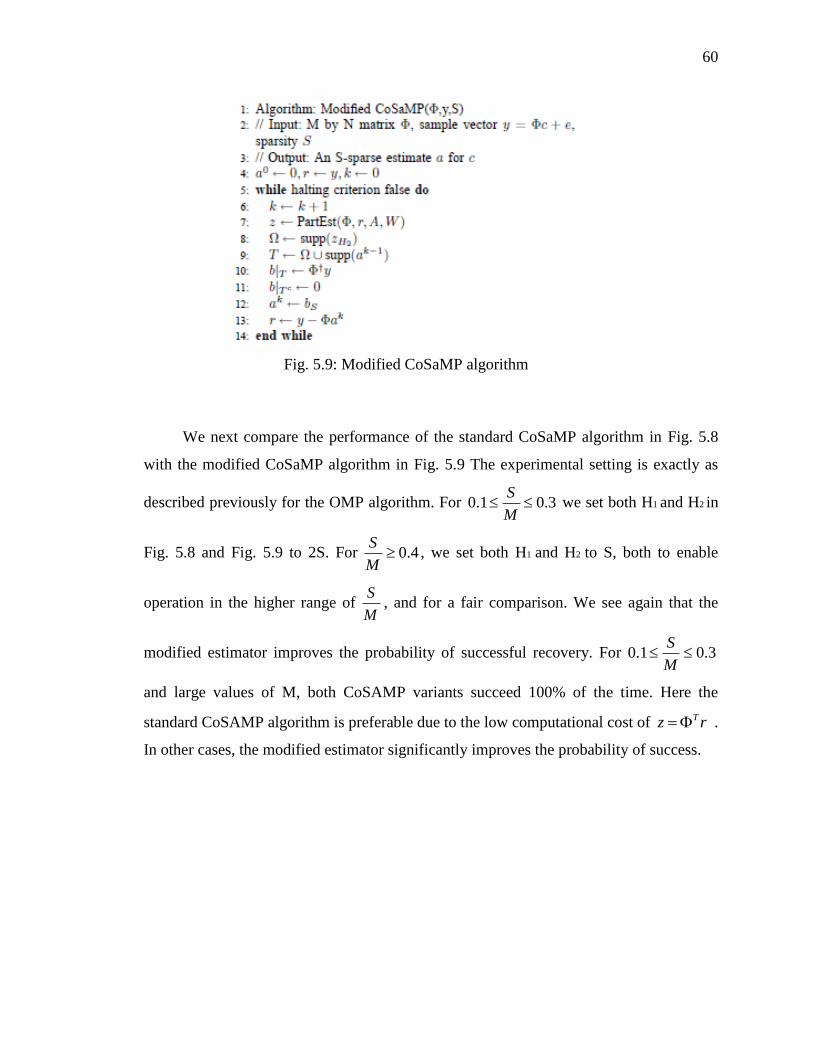
60
We next compare the performance of the standard CoSaMP algorithm in Fig. 5.8
with the modified CoSaMP algorithm in Fig. 5.9 The experimental setting is exactly as
described previously for the OMP algorithm. For 0.1 0.3S
M we set both H1 and H2 in
Fig. 5.8 and Fig. 5.9 to 2S. For 0.4S
M , we set both H1 and H2 to S, both to enable
operation in the higher range of S
M, and for a fair comparison. We see again that the
modified estimator improves the probability of successful recovery. For 0.1 0.3S
M
and large values of M, both CoSAMP variants succeed 100% of the time. Here the
standard CoSAMP algorithm is preferable due to the low computational cost of Tz r .
In other cases, the modified estimator significantly improves the probability of success.
Fig. 5.9: Modified CoSaMP algorithm

61
Table 5.4: Fraction of Successful Recoveries for Standard CoSaMP Algorithm with
N=256
Number of Samples M
S/M ratio 50 100 150 200 250
0.5 0 0 0 0 0.83
0.4 0 0 0.15 0.85 1.0
0.3 0.05 0.43 0.98 1.0 1.0
0.2 0.62 0.99 1.0 1.0 1.0
0.1 1.0 1.0 1.0 1.0 1.0
Table 5.5: Fraction of Successful Recoveries for Modified CoSaMP Algorithm with
N=256
Number of Samples M
S/M ratio 50 100 150 200 250
0.5 0 0 0.03 0.87 1.0
0.4 0 0.04 0.73 1.0 1.0
0.3 0.07 0.78 1.0 1.0 1.0
0.2 0.79 1.0 1.0 1.0 1.0
0.1 1.0 1.0 1.0 1.0 1.0

62
6. SUMMARY
This thesis contributes novel algorithms for image superresolution, image fusion,
and content based retrieval based on compressive sensing, as well as an estimator that
improves the Matching Pursuit family of algorithms.
Three algorithms are developed for image fusion that show better spectral fidelity
properties than conventional methods such as Principal Component Analysis (PCA),
while preserving the spatial quality of the high resolution panchromatic image. A
modified version of the Brovey transform is also developed that has far less color
distortion than the standard transform, while maintaining the simplicity and low
computational complexity of the standard algorithm. The results of these novel
algorithms are compared to existing methods using the Correlation Coefficient, Spectral
Angle Mapper and ERGAS measures.
Compressive sensing is used to reduce the storage needed for image databases
used for Content Based Image Retrieval. A novel feature vector is defined that uses
projections (dot product) values of the image with patterns. The feature vector is used to
reconstruct the image as needed, instead of having to compress and store the full image.
This significantly reduces the size of the database, since the storage needed for the
feature vector and the reconstruction error is much less than that needed to store the
feature vector and the entire image.
The thesis also develops a novel estimator that uses partial inversions for subsets
of columns of the sampling matrix. The individual estimates are combined to produce a
more accurate estimator for the nonzero locations of the signal vectors. This estimator
can improve the performance of all the Matching Pursuit type algorithms that are
commonly used for compressive sensing recovery.

LIST OF REFERENCES

63
LIST OF REFERENCES
[1] G.K. Wallace, "The JPEG Still Picture Compression Standard," Communications of
the ACM, vol. 34, no. 4, pp. 30-44, 1991.
[2] D.S. Taubman and M.W. Marcellin, JPEG2000 :Image Compression Fundamentals,
Standards and Practice. Boston: Kluwer Academic Publishers, 2002.
[3] A. Said and W. Pearlman, "A New Fast and Efficient Image Codec Based on Set
Partitioning in Hierarchical Trees," IEEE Transactions on Circuits and Systems for
Video Technology, vol. 6, pp. 243-250, 1996.
[4] B. Haskell, A. Puri and A.N Netravali, Digital Video: An Introduction to MPEG2.
London, UK: Chapman and Hall, 1996.
[5] I. Richardson, The H.264 Advanced Video Compression Standard.: John Wiley and
Sons, 2010.
[6] E. Candes, "The Restricted Isometry Property and its Implications for Compressed
Sensing," Compte Rendus de l'Academie des Sciences, Paris, vol. Series I,346, pp.
589-592, 2008.
[7] E. Candes and T. Tao, "Near Optimal Signal Recovery from Random Projections:
Universal Encoding Strategies?," IEEE Trans. on Information Theory, vol. 52, no.
12, pp. pp. 5406 - 5425, December 2006.
[8] E. Candes and J. Romberg, "Sparsity and Incoherence in Compressive Sampling,"
Inverse Problems, vol. 23, no. 3, pp. 969-985, 2007.
[9] J. Tropp and A. Gilbert, "Signal Recovery from Random Measurements via
Orthogonal Matching Pursuit," IEEE Trans. on Information Theory, vol. 53, no. 12,
pp. 4655-4666, December 2007.
[10] D. Needell and J. Tropp, "CoSaMP: Iterative Signal Recovery from Incomplete and
Accurate Samples," Applied and Computational Harmonic Analysis, vol. 26, pp.
301-321, 2009.
[11] D. Donoho, Y. Tsaig, I. Drori, and J.L. Starck, "Sparse Solution of Underdetermined
Linear Equations by Stagewise Orthogonal Matching Pursuit," preprint.

64
[12] D. Wei and O. Milenkovic, "Subspace Pursuit for Compressive Sensing Signal
Reconstruction," IEEE Transactions on Information Theory, vol. 55, no. 5, pp. 2230-
2249, 2009.
[13] D. Needell and R. Vershynin, "Uniform Uncertainty Principle and Signal Recovery
via Regularized Orthogonal Matching Pursuit," Foundations of Computational
Mathematics, no. 9, pp. 317-334, 2009.
[14] H. Rauhut, "On the Impossibility of Uniform Sparse Reconstruction Using Greedy
Methods," Sampling Theory Signal and Image Processing, 2008.
[15] J. Wright, A. Yang, A. Ganesh, S. Sastry and Y. Ma, "Robust Face Recognition via
Sparse Representation," IEEE Transactions on Pattern Analysis and Machine
intelligence, February 2009.
[16] S. Farsiu, D. Robinson, M. Elad, and P. Milanfar, "Advances and challenges in
super-resolution," International Journal of Imaging Systems and Technology, vol.
14, no. 2, pp. 47-57, 2004.
[17] T. Tu, S. Su, S. Shyu, and P. Huang, "A New Look at IHS-like Image Fusion
Methods," Information Fusion, vol. 2, no. 3, pp. 177-186, September 2001.
[18] a. R. Gillespie, A. Kahle, and R. Walker, "Color Enhancement of Highly Correlated
Images-II. Channel Ratio and Chromaticity Transformation Techniques," Remote
Sensing of Environment, vol. 22, pp. 343-365, 1987.
[19] P.S. Chavez, S.C. Sides, and J.A. Anderson, "Comparison of three different methods
to merge multiresolution and multispectral data :Landsat TM and SPOT
Panchromatic," Photogrammetric Engineering and Remote Sensing, vol. 57, no. 3,
pp. 311-316, 1985.
[20] H. Li, B. S. Manjunath, and S. K. Mitra, "Multisensor Image Fusion using the
Wavelet Transform," Graphical Models and Image Processing, vol. 57, pp. 234-245,
1995.
[21] B. Aiazzi, L. Alparone, S. Baronti, and A. Garzelli, "Context-Driven Fusion of High
Spatial and Spectral lResolution Images Based on Oversampled Multiresolution
Analysis," IEEE Transactions on Geoscience and Remote Sensing, vol. 40, no. 10,
pp. 3230-3239, October 2002.
[22] Stephane Mallat, A Wavelet Tour of Signal Processing.: Academic Press, 1998.
[23] L. Wald, "Quality of High Resolution Synthesised Images: Is there a Simple
Criterion ?," in Proc. Third Conference on "Fusion of Earth data: merging point
measurements, raster maps and remotely sensed images", Sophia Antipolis, France,
2000, pp. 99-103.

65
[24] R. Datta, D. Joshi, J. Li, and J. Wang, "Image Retrieval: Ideas, Influences, and
Trends of the New Age," ACM Computing Surveys, vol. 40, no. 2, pp. 1-60, 2008.
[25] A. Smeulders, M. Worring, S. Santini , A. Gupta, and R. Jain, "Content-based Image
Retrieval at the End of the Early Years," IEEE Trans. Pat. Anal. Mach., vol. 22, no.
2, pp. 1349-1380, 2000.
[26] P.M. Kelly, T.M. Cannon, and D.R. Hush, "Query by Image Example: The
CANDID approach," in SPIE Vol.2420 Storage and Retrieval for Image and Video
Databases III, 1995, pp. 238-248.
[27] F. Korn, N. Sidiropolous, C. Faloutsos, E. Siegel, and Z. Protopapas, "Fast and
effective retrieval of medical tumor shapes," IEEE Transactions on Knowledge and
Data Engineering, no. 6, pp. 889-904, 1998.
[28] G. Healey and A. Jain, "Retrieving Multispectral Satellite images using Physics
Based Invariant Representations," IEEE Transactions on Pattern Analysis and
Machine Intelligence, vol. 18, pp. 842-848, August 1996.
[29] J.Li and R. Narayanan, "Integrated Spectral and Spatial Information Mining in
Remote Sensing Imagery," IEEE Transactions on Geoscience and Remote Sensing,
vol. 42, pp. 673-385, march 2004.
[30] W. Johnson and J. Lindenstrauss, "Extensions of Lipschitz maps into Hilbert space,"
Contemp. Math, pp. 189-206, 1984.
[31] A. Divekar and O. Ersoy, "Compact Storage of Correlated Data by Content Based
Retrieval," in Proc. 43rd Asilomar Conference on Signals, Systems, and Computers,
Pacific Grove,CA, 2009.
[32] S. Mallat and Z. Zhang, "Matching pursuits with time-frequency dictionaries," IEEE
Transactions on Signal Processing, vol. 41, no. 12, pp. 3397-3415, 1993.
[33] Y. Luo and R. Duraiswami, "Efficient parallel non-negative least squares on the
GPU," SIAM Journal on Scientific Computing, Copper Mountain Special Edition ,
2010.
[34] l1-magic. [Online]. http://www.acm.caltech.edu/l1magic/
[35] M. Abramowitz and I. Stegun, Handbook of Mathematical Functions with Formulas,
Graphs, and Mathematical Tables, 9th ed. New York: Dover, 1964.
[36] V. Marchenko and L. Pastur, "Distribution of eigenvalues for some sets of random
matrices," Mat. Sb. (N.S.), vol. 72, no. 114, pp. 507-536, 1967.
[37] S. Ferrando, E. Doolittle, A.J. Bernal, and L. Bernal, "Probabilistic Matching Pursuit
with Gabor Dictionaries," Signal Processing, vol. 80, pp. 2099-2120, 2000.

VITA

66
VITA
Atul Divekar received his Bachelor‟s degree (B.E.) in Computer Engineering from
the Government College of Engineering, Pune, affiliated to the University of Pune, India,
in August 1999. He received the Master of Science degree in Electrical and Computer
Engineering from Purdue University, West Lafayette, Indiana, USA, in May 2001. His
research interests include signal and image processing, digital video and inverse
problems.