theory, benefits and limitations - njf – norsk ... · response spectrum analysis . theory,...

Response Spectrum Analysis Theory, Benefits and Limitations

Emrah Erduran, PhD NORSAR / International Center of Geohazards (ICG), Kjeller, Norway

Table of contents

1. Introduction

2. Design spectrum for elastic analysis

3. Free Vibration

3.1. SDOF

4.1. MDOF

4. Modal Analysis under Earthquake Forces

5. Response Spectrum Analysis (RSA)

6. RSA in EC-8

7. Tutorial

8. Concluding Remarks

Structural Analysis under Seismic Action

The aim of structural analysis under seismic action is to compute the design actions (forces and displacements) on the building components and the entire system

G + ΨEi ⋅ Q General types of analysis methods specified in EC8:

linear-elastic methods:

(1) lateral force method of analysis

(2) response spectrum analysis

non-linear (inelastic) methods

(3) non-linear static ('pushover') analysis

(4) non-linear time history analysis

i j

lpl lpl

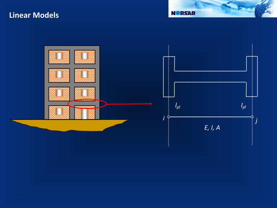
Linear Models

E, I, A

i j

plastic hinge region

lpl lpl

lpl = 0.5∙d to d

with: d - depth of section

Moment

Curvature

Non-linear Models

Curvature

Mom

ent

E, I, A

to avoid explicit inelastic structural analysis in design, the capacity of the structure to dissipate energy is accounted for by using a reduced response spectrum by q

q is an approximation of the ratio of seismic forces that the structure would experience if its response would be completely elastic to the seismic forces used for the design

for 0 ≤ T ≤ TB :

for TB ≤ T ≤ TC :

for TC ≤ T ≤ TD :

for TD ≤ T ≤ 4 s :

−⋅+⋅⋅= )

.()(

3252

32

qTTSaTS

Bgd

qSaTS gd

52.)( ⋅⋅=

⋅⋅⋅=

TT

qSa C

g52.

⋅⋅⋅⋅= 2

52T

TTq

Sa DCg

.

Design spectrum for elastic analysis

Period T [sec]

Spec

tral

acc

eler

atio

n S d

q = 1

q = 2

q = 4

TB TC TD ga⋅≥ β

)(TSd

)(TSd

ga⋅≥ β

with: β = 0.20 (lower bound factor)

(EN 1998-1:2004 3.2.2.2)

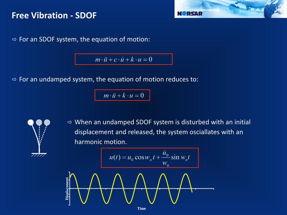
Free Vibration - SDOF

For an SDOF system, the equation of motion:

For an undamped system, the equation of motion reduces to:

When an undamped SDOF system is disturbed with an initial displacement and released, the system osciallates with an harmonic motion.

Disp

lace

men

t

Time

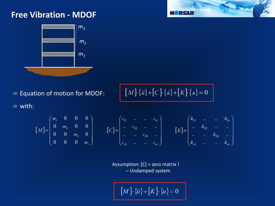
Free Vibration - MDOF

Equation of motion for MDOF:

with:

Assumption: [C] = zero matrix ! – Undamped system

[ ] { } [ ] { } [ ] { } 0=⋅+⋅+⋅ uKuCuM

[ ]

=

imm

mm

M

000000000000

3

2

1

[ ]

=

nnn

n

ccc

ccc

C

................

....

1

33

22

111

[ ]

=

nnn

n

kkk

kkk

K

................

....

1

33

22

111

m2

m3

m1


Contrary to SDOF systems, for a MDOF system, the motion of each mass (or each floor) is NOT a simple harmonic motion, when an arbitrary initial deflection is applied to the system.

An associated period (or frequency) cannot be defined.

An undamped MDOF will undergo simple harmonic motion with an associated frequency only if the initial deformations are arranged in an approprioate distribution

m2

m3

m1

φn,1

φj+1,1

φj,1

φn,2

φj+1,2

φj,2

φn,3

φj+1,3

φj,3

NATURAL MODES OF VIBRATION

or

MODE SHAPES


At any given instant:

wn: natural circular frequency of vibration

Tn: natural period of vibration; time required for one cycle of simple harmonic motion

m2

m3

m1

φn,1

φj+1,1

φj,1

φn,2

φj+1,2

φj,2

φn,3

φj+1,3

φj,3

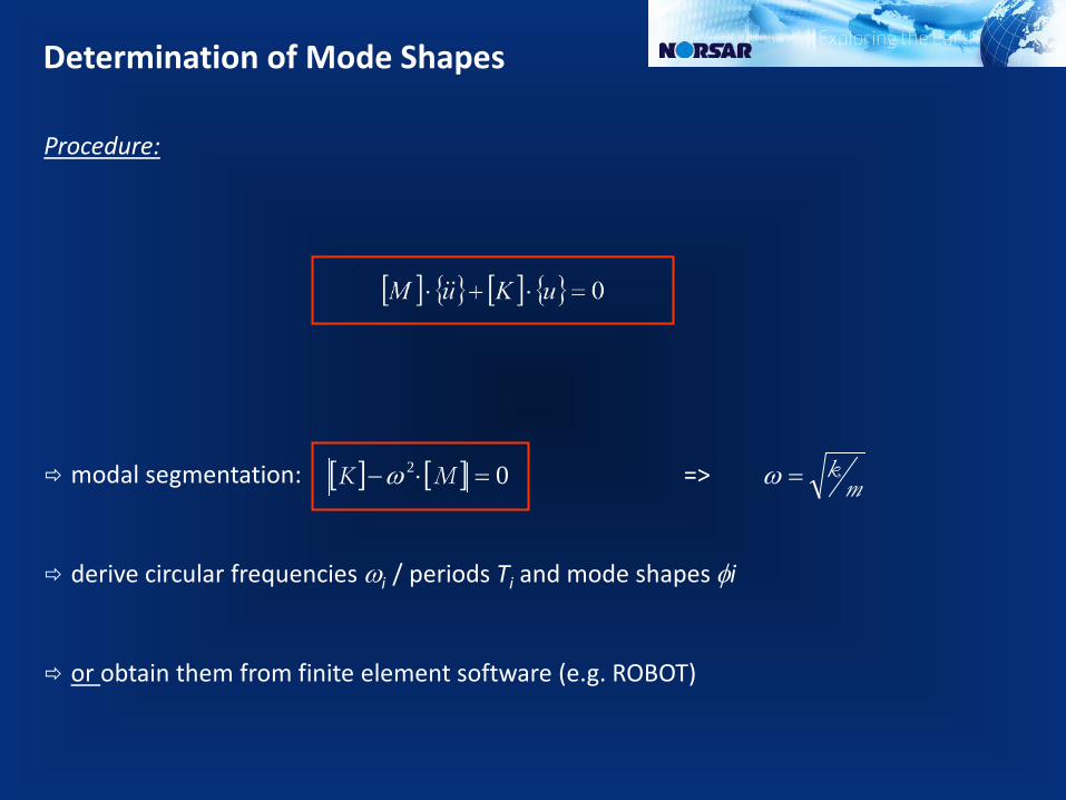
Determination of Mode Shapes

Procedure:

modal segmentation: =>

derive circular frequencies ωi / periods Ti and mode shapes φi

or obtain them from finite element software (e.g. ROBOT)

[ ] [ ] 02 =⋅− MK ω mk=ω

Modal Analysis of MDOF systems under earthquake forces

=

m2

m3

m1

φn,1

φj+1,1

φj,1

φn,2

φj+1,2

φj,2

φn,3

φj+1,3

φj,3

m2

m3

m1 T1

T2 T3


=

φn,1

φj+1,1

φj,1

φn,2

φj+1,2

φj,2

φn,3

φj+1,3

φj,3

m2

m3

m1

T1

T2

T3

qi(t) can be computed fairly easily!


Modal analysis of MDOF systems allows us to conduct a simplified analysis instead of solving a system of nxn differential equations.

However, we still need to solve n differential equations!!!

Modal analysis provides us with the response parameters (e.g. member forces, displacements, etc...) at every time step of an earthquake record.

Typically, this time step is between 0.005 seconds and 0.02 seconds.

Do we really need this information?

ENGINEERS NEED TO KNOW ONLY THE MAXIMUM PROBABLE ACTION FOR DESIGN!

RESPONSE SPECTRUM!

Excursion

Response spectrum:

used in earthquake engineering (exclusively)

describes the maximum response of a SDOF system to a particular input motion (i.e. the respective accelerogram)

dependent on damping ratio ξ (1–10 %)

response spectra reflect the maximum response to simple structures (SDOF)

T1 T2 T3 T4 T5 T6 T7

Sa,1

Sa,2 Sa,3

Sa,4

Sa,5

Sa,6

Sa,7

Spec

tral a

ccel

erat

ion

S a

Period T

maximum value

response action

earthquake impact

Response spectrum:

Response Spectrum Analysis

Procedure:

Given: - circular frequencies ωi / periods Ti

- mode shapes φi

modal participation factors γi :

design spectral accelerations Sa(Ti ) for each mode i :

{ }

= +

1

11

1

1

,

,

,

n

j

j

φφφ

φ

∑

∑

=

=

⋅

⋅= n

jijj

n

jijj

i

m

m

1

2

1

,

,

φ

φγ

φn,1

φj+1,1

φj,1

T1

Period T [sec]

Spec

tral

acc

eler

atio

n S a

T2 T3 T1

Sa,d (T3)

Sa,d (T2) Sa.d (T1)

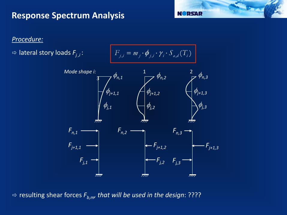
Response Spectrum Analysis

Procedure:

lateral story loads Fj ,i :

)(,,, idaiijjij TSmF ⋅⋅⋅= γφ

Mode shape i: 1 2 3

Fn,1

Fj+1,1

Fj,1

Fn,2

Fj+1,2

Fj,2

Fn,3

Fj+1,3

Fj,3

φn,1

φj+1,1

φj,1

φn,2

φj+1,2

φj,2

φn,3

φj+1,3

φj,3

resulting shear forces Fb,m, that will be used in the design: ????

Modal Combination Rules

Square root of sum of squares (SRSS):

Simple

Fairly ‘accurate’ for buildings with well-seperated frequencies.

Should be avoided if the modal frequencies are close to each other.

Absolute Sum(ABSSUM):

Very Simple (Primitive (?))

Conservative... REALLY Conservative!!

Modal Combination Rules

Complete Quadratic Combination:

Mathematically complex

Leads to the most reliable solution for buildings with closely spaced natural frequencies .

... as well as well-seperated frequencies

ρn,m is the cross-modal coefficient

Response spectrum analysis in EC-8

Criteria:

shall be applied if the criteria for analysis method (1) are not fulfilled, this means if:

4 ⋅ TC T1 > 2.0 sec

Fb

1st mode

response of all modes shall be considered that contribute significantly to the global building response (i.e., important for buildings of a certain height)

those modes shall be considered for which:

(1) the sum of the modal masses is at least 90% of the total building mass or

(2) the modal mass is larger than 5% of the total building mass

∑mi ≥ 0.9 ⋅ mtot

mi ≥ 0.05 ⋅ mtot

(EN 1998-1:2004 4.3.3.3)

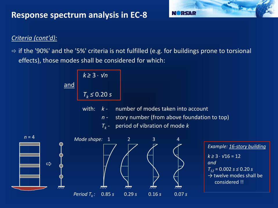
Response spectrum analysis in EC-8

Criteria (cont'd):

if the '90%' and the '5%' criteria is not fulfilled (e.g. for buildings prone to torsional effects), those modes shall be considered for which:

with: k - number of modes taken into account n - story number (from above foundation to top) Tk - period of vibration of mode k

n = 4

k ≥ 3 ⋅ √n and Tk ≤ 0.20 s

Mode shape: 1 2 3 4

Period Tk : 0.85 s 0.29 s 0.16 s 0.07 s

Example: 16-story building

k ≥ 3 ⋅ √16 = 12 and T12 = 0.002 s ≤ 0.20 s → twelve modes shall be

considered !!

Methods of analysis

General types of analysis methods specified in EC8:

Regularity Allowed simplification Behavior factor (for linear analysis) Plan Elevation Model Linear-elastic analysis

● ● planar

lateral force reference value

● ○ modal decreased value (⋅0.8)

○ ● spatial

lateral force reference value

○ ○ modal decreased value (⋅0.8)

(EN 1998-1:2004 4.2.3)

3-story RC frame building (residential use) behavior factor q = 4 ground motion: agR = 0.3 g residential use: γI = 1.0 structural parameters: E = 2.1 ⋅ 108 kN/m2 I = 2.679 ⋅ 10-5 m4 h = 3.0 m k = 12 ⋅ EI/h3

m = 50 tons = 50 kNs2/m

Tutorial – VIII – 'Modal RS method'

1. Setting up the differential equation of motion:

cf. Tutorial 4.2

m3 = m

m2 = 1.5m

m1 = 2m

h h h

k3 = k

k2 = 2k

k1 = 3k

[ ] { } [ ] { } [ ] { } 0=⋅+⋅+⋅ uKuCuM if [C] = 0 : [ ] { } [ ] { } 0=⋅+⋅ uKuM

[ ]

⋅=

=

1000510002

000000

3

2

1

.mm

mm

M [ ]

−−−

−⋅=

−−+−

−+=

110132

025

0

0

33

3322

221

kkkkkkk

kkkK


2. Modal segmentation:

cf. Tutorial 4.2

⇒ [ ] [ ] 02 =⋅− MK ω0

05132

0225

2

2

2

=−−−−−

−−

ωω

ω

mkkkmkk

kmk.

3. Modal circular frequencies ωi and periods Ti :

ω1 = 4.19 s-1 → T1 = 1.50 sec ω2 = 8.97 s-1 → T2 = 0.70 sec ω3 = 13.3 s-1 → T3 = 0.47 sec

4. Eigenmodes:

{ }

=

0016440300

1

...

φ { }

−−

=00160106760

2

...

φ { }

−=

001572

472

3

..

.φ


5. Modal participation factors γi :

cf. Tutorial 4.2

α1 = 100 ⋅ 0.3 + 75 ⋅ 0.644 + 50 ⋅ 1.0 = 128.3 kNs2/m α2 = –100 ⋅ 0.676 – 75 ⋅ 0.601 + 50 ⋅ 1.0 = -62.7 kNs2/m α3 = 100 ⋅ 2.47 – 75 ⋅ 2.57 + 50 ⋅ 1.0 = 104.3 kNs2/m M1

* = 100 ⋅ 0.32 + 75 ⋅ 0.6442 + 50 ⋅ 1.02 = 90.0 kNs2/m M2

* = 100 ⋅ 0.6762 + 75 ⋅ 0.6012 + 50 ⋅ 1.02 = 122.8 kNs2/m M3

* = 100 ⋅ 2.472 + 75 ⋅ 2.572 + 50 ⋅ 1.02 = 1155.0 kNs2/m → γ1 = 128.3 / 90.0 = 1.426 → γ2 = -62.7 / 122.8 = –0.511 → γ3 = 104.3 / 1155.0 = 0.090

*

,

,

i

in

jijj

n

jijj

i Mm

mα

φ

φγ =

⋅

⋅=

∑

∑

=

=

1

2

1


6. Design spectral accelerations Sa(Ti ) for each mode i : T1 = 1.50 sec : Check: Sa,d (T) = 0.846 m/s2 ≥ β ∙ ag = 0.20 ∙ 2.943 = 0.5886 m/s2 T2 = 0.70 sec : Check: Sa,d (T) = 1.813 m/s2 ≥ β ∙ ag = 0.20 ∙ 2.943 = 0.5886 m/s2 T3 = 0.47 sec :

cf. Tutorial 4.2

2

1

846050160

045215101943252 sm

TT

qSaTS C

gda /...

.

..)..(

.)(, =

⋅⋅⋅⋅=

⋅⋅⋅=

2

1

81317060

045215101943252 sm

TT

qSaTS C

gda /...

.

..)..(

.)(, =

⋅⋅⋅⋅=

⋅⋅⋅=

21152045215101943252 sm

qSaTS gda /.

.

..)..(

.)(, =⋅⋅⋅=⋅⋅=


5. Lateral story loads Fj,i : F1,1

= 100 ⋅ 0.30 ⋅ 1.426 ⋅ 0.846 = 36.2 kN F2,1

= 75 ⋅ 0.644 ⋅ 1.426 ⋅ 0.846 = 58.3 kN F3,1

= 50 ⋅ 1.00 ⋅ 1.426 ⋅ 0.846 = 60.3 kN F1,2

= 100 ⋅ (–0.676) ⋅ (–0.511) ⋅ 1.813 = 62.6 kN F2,2

= 75 ⋅ (–0.601) ⋅ (–0.511) ⋅ 1.813 = 41.8 kN F3,2

= 50 ⋅ 1.00 ⋅ (–0.511) ⋅ 1.813 = –46.3 kN F1,3

= 100 ⋅ 2.47 ⋅ 0.090 ⋅ 2.115 = 47.0 kN F2,3

= 75 ⋅ (–2.57) ⋅ 0.090 ⋅ 2.115 = –36.7 kN F3,3

= 50 ⋅ 1.00 ⋅ 0.090 ⋅ 2.115 = 9.5 kN

cf. Tutorial 4.2

)(,,, idaiijjij TSmF ⋅⋅⋅= γφF3,1= 60.3

F2,1 = 58.3

F1,1 = 36.2

F3,2 = –46.3

F2,2 = 41.8

F1,2 = 62.6

F3,3 = 9.5

F2,3 = –36.7

F1,3 = 47.0


5. Maximum shear forces Fb :

cf. Tutorial 4.2

60.3

118.6

154.8

-46.3

-4.5

58.1

9.5

-27.2

19.8

76.6

121.7

166.5

⇒

2

1imb

n

imb FF ,,, ∑

=

=

Conclusion

• Response Spectrum Analysis (RSA) is an elastic method of analysis and lies in between equivalent force method of analysis and nonlinear analysis methods in terms of complexity.

• RSA is based on the structural dynamics theory and can be derived from the basic principles (e.g. Equation of motion).

• RSA, unlike equivalent force method, considers the influence of several modes on the seismic behaviour of the building.

• Damping of the structures is inherently taken into account by using a design (or response) spectrum with a predefined damping level.

• The maximum response of each mode is an exact solution.

• The sole approximation used in RSA is the combination of modal responses.

Conclusion (cont.d)

• ABSSUM is the most conservative modal combination rul. Too conservative?

• SRSS is the most popular modal combination rule due to its simplicity and ‘accuracy’ for buildings with well-seperated frequencies.

• CQC is regarded as the most viable option for any structure.

theory, benefits and limitations - njf – norsk ... · response spectrum analysis . theory,...

Documents