theory introduction to programming languages
TRANSCRIPT
7/3/2019 Theory Introduction to Programming Languages
http://slidepdf.com/reader/full/theory-introduction-to-programming-languages-5584618bb4249 1/233
Theory
Introduction toProgramming Languages
Anthony A. Aaby
DRAFT Version 0.9. Edited July 15, 2004
7/3/2019 Theory Introduction to Programming Languages
http://slidepdf.com/reader/full/theory-introduction-to-programming-languages-5584618bb4249 2/233
Copyright c 1992-2004 by Anthony A. Aaby
Walla Walla College204 S. College Ave.College Place, WA 99324E-mail: [email protected]
This work is licensed under the Creative Commons Attribution License. To viewa copy of this license, visit http://creativecommons.org/licenses/by/2.0/ or senda letter to Creative Commons, 559 Nathan Abbott Way, Stanford, California94305, USA.
This book is distributed in the hope it will be useful, but without any warranty;without even the implied warranty of merchantability or fitness for a particularpurpose.
No explicit permission is required from the author for reproduction of this bookin any medium, physical or electronic.
The author solicits collaboration with others on the elaboration and extensionof the material in this text. Users are invited to suggest and contribute materialfor inclusion in future versions provided it is offered under compatible copyrightprovisions. The most current version of this text and LATEXsource is availableat http://www.cs.wwc.edu/~aabyan/Logic/index.html.

7/3/2019 Theory Introduction to Programming Languages
http://slidepdf.com/reader/full/theory-introduction-to-programming-languages-5584618bb4249 3/233
To Ogden and Amy Aaby

7/3/2019 Theory Introduction to Programming Languages
http://slidepdf.com/reader/full/theory-introduction-to-programming-languages-5584618bb4249 4/233
iv
7/3/2019 Theory Introduction to Programming Languages
http://slidepdf.com/reader/full/theory-introduction-to-programming-languages-5584618bb4249 5/233
Preface
It is the purpose of this text to explain the concepts underlying programminglanguages and to examine the major language paradigms that use these con-
cepts.Programming languages can be understood in terms of a relatively small numberof concepts. In particular, a programming language is syntactic realization of one or more computational models. The relationship between the syntax andthe computational model is provided by a semantic description. Semanticsprovide meaning to programs. The computational model provides much of theintuition behind the construction of programs. When a programming languageis faithful to the computational model, programs can be more easily written andunderstood.
The fundamental concepts are supported bindings, abstraction and generaliza-tion. Concepts so fundamental that they are included in virtually every pro-gramming language. These concepts support the human facility for simile and
metaphor which are so necessary in problem solving and in managing complex-ity.
Programming languages are also shaped by pragmatic considerations. Formostamong these considerations are safety, efficiency and applicability. In somelanguages these external forces have played a more important role in shaping thelanguage than the computational model to the point of distorting the languageand actually limiting the applicability of the language. There are several distinctcomputational models — imperative, functional, and logic. While these modelsare equivalent (all computable functions may be defined in each model), thereare pragmatic reasons for prefering one model over the another.
This text is designed to formalize and consolidate the knowledge of programminglanguages gained in the introductory courses a computer science curriculum
and to provide a base for further studies in the semantics and translation of programming languages. It aims at covering the bulk of the subject area PL:Programming Languages as described in the “ACM/IEEE Computing Curricula1991.”
v
7/3/2019 Theory Introduction to Programming Languages
http://slidepdf.com/reader/full/theory-introduction-to-programming-languages-5584618bb4249 6/233
Special Features of the Text
The following are significant features of the text as compared to the standardtexts.
• Syntax: an introduction to regular expressions, scanning, context-freegrammars, parsing, attribute grammars and abstract grammars.
• Semantics: introductory treatment of algebraic, axiomatic, denotationaland operational semantics.
• Programming Paradigms: the major programming paradigms are promi-nently featured.
– Functional: includes an introduction to the lambda calculus and usesthe programming languages Scheme and Haskell for examples
– Logic: includes an emphasis on the formal semantics of Prolog
– Concurrent: introduces both low- and high-level notations for con-curency, stresses the importance of the logic and functional paradigmsin the debate on concurrency, and uses the programming languageSR for examples.
– Object-oriented: uses the programming language Modula-3 for ex-amples
• Language design principles: Twenty some programming language designprinciples are given prominence. In particular, the importance of abstrac-
tion and generalization is stressed.
Readership
This book is intended as an undergraduate text in the theory of programminglanguages. To gain maximum benefit from the text, the reader should have ex-perience in a high-level programming language such as Pascal, Modula-2, C++,ML or Common Lisp, machine organization and programming, and discretemathematics.
Programming is not a spectator sport. To gain maximum benefit from the text,the reader should construct programs in each of the paradigms, write semanticspecifications; and implement a small programming language.
Organization
Since the subject area PL: Programming Languages as described in the “ACM/IEEEComputing Curricula 1991” consists of a minimum of 47 hours of lecture, thetext contains considerably more material than can be covered in a single course.
vi
7/3/2019 Theory Introduction to Programming Languages
http://slidepdf.com/reader/full/theory-introduction-to-programming-languages-5584618bb4249 7/233
The first part of the text consists of chapters 1–3. Chapter 1 is an overviewof the text, an introduction to the areas of discussion. It introduces the keyconcepts: the models of computation, syntax, semantics, abstraction, general-ization and pragmatics which are elaborated in the rest of the text. Chapter2 introduces context-free grammars, regular expressions, and attribute gram-mars. Context-free grammars are utilized throughout the text but the othersections are optional. Chapter 3 introduces semantics: algebraic, axiomatic,denotational and operational. While the chapter is optional, I introduce al-gebraic semantics in conjunction with abstract types and axiomatic semanticswith imperative programming.
Chapter 4 is a formal treatment of abstraction and generalization as used inprogramming languages.
Chapter 5 deals with values, types, type constructors and type systems. Chapter
6 deals with environments, block structure and scope rules. Chapter 7 dealswith the functional model of computation. It introduces the lambda calculusand examines Scheme and Haskell. Chapter 8 deals with the logic model of computation. It introduces Horn clause logic, resolution and unification andexamines Prolog. Chapter 9 deals with the imperative model of computation.Features of several imperative programming languages are examined. Variousparameter passing mechanisms should be discussed in conjunction with thischapter. Chapter 10 deals with the concurrent model of programming. Itsprimary emphasis is from the imperative point of view. Chapter 11 is a furtherelaboration of the concepts of abstraction and generalization in the moduleconcept. It is preparatory for Chapter 12. Chapter 12 deals with the object-oriented model of programming. Its primary emphasis is from the imperativepoint of view. Features of Smalltalk, C++ and Modula-3 provide examples.
Chapter 13 deals with pragmatic issues and implementation details. It may beread in conjunction with earlier chapters. Chapter 14 deals with programmingenvironments, Chapter 15 deals with the evaluation of programming languagesand a review of programming language design principles. Chapter 16 containsa short history of programming languages.
Pedagogy
The text provides pedagogical support through various exercises and labora-tory projects. Some of the projects are suitable for small group assignments.The exercises include programming exercises in various programming languages.
Some are designed to give the student familiarity with a programming conceptsuch as modules, others require the student to construct an implementation of aprogramming language concept. For the student to gain maximum benefit fromthe text, the student should have access to a logic programming language (suchas Prolog), a modern functional language (such as Scheme, ML or Haskell),a concurrent programming language (Ada, SR, or Occam), an object-orientedprogramming language (C++, Small-Talk, Eiffel, or Modula-3), and a modern
vii
7/3/2019 Theory Introduction to Programming Languages
http://slidepdf.com/reader/full/theory-introduction-to-programming-languages-5584618bb4249 8/233
programming environment and programming tools. Free versions of Prolog,ML, Haskell, SR, and Modula-3 are available from one or more ftp sites and arerecommended.
The instructor’s manual contains lecture outlines and illustrations from the textwhich may be transferred to transparencies. There is also a laboratory manualwhich provides short introductions to Lex, Yacc, Prolog, Haskell, Modula-3, andSR.
The text has been used as a semester course with a weekly two hour lab. Itsapproach reflects the core area of programming languages as described in the re-port Computing as a Discipline in CACM January 1989 Volume 32 Number1.
Knowledge Unit Mapping
To assist in curriculum development, the follow mapping of the ACM knowledgeunits to the text is provided.
Knowledge Unit Chapter(s)PL1: History 6,7,8,9,11PL2: Virtual Machines 2,6,7,8,13PL3: Data Types 5,13PL4: Sequence Control 9,10PL5: Data Control 5,11,12PL6: Run-time 2,13PL7: Regular Expressions 2
PL8: Context-free grammars 2PL9: Translation 2PL10: Semantics 3PL11: Programming Paradigms 1,7,8,9,10,12PL12: Parallel Constructs 10SE3: Specifications 3
Acknowledgements
There are several programming texts that have influenced this work in partic-ular, texts by Hehner, Tennent, Pratt, and Sethi. I am grateful to my CS208classes at Bucknell for their comments on preliminary versions of this material
and to Bucknell University for providing the excellent environment in and withwhich to develop this text.
AA 1992
viii
7/3/2019 Theory Introduction to Programming Languages
http://slidepdf.com/reader/full/theory-introduction-to-programming-languages-5584618bb4249 9/233
Contents
Preface v
1 Introduction 1
1.1 Models of Computation . . . . . . . . . . . . . . . . . . . . . . . 3
1.2 Syntax and Semantics . . . . . . . . . . . . . . . . . . . . . . . . 7
1.3 Pragmatics . . . . . . . . . . . . . . . . . . . . . . . . . . . . . . 7
1.4 Language Design Principles . . . . . . . . . . . . . . . . . . . . . 8
1.5 Further Reading . . . . . . . . . . . . . . . . . . . . . . . . . . . 10
1.6 Exercises . . . . . . . . . . . . . . . . . . . . . . . . . . . . . . . 11
2 Syntax 13
2.1 Context-Free Grammars . . . . . . . . . . . . . . . . . . . . . . . 14
2.2 Regular Expressions . . . . . . . . . . . . . . . . . . . . . . . . . 21
2.3 Attribute Grammars and Static Semantics . . . . . . . . . . . . . 23
2.4 Further Reading . . . . . . . . . . . . . . . . . . . . . . . . . . . 24
2.5 Exercises . . . . . . . . . . . . . . . . . . . . . . . . . . . . . . . 25
3 Semantics 27
3.1 Algebraic Semantics . . . . . . . . . . . . . . . . . . . . . . . . . 28
3.2 Axiomatic Semantics . . . . . . . . . . . . . . . . . . . . . . . . . 29
3.3 Denotational Semantics . . . . . . . . . . . . . . . . . . . . . . . 363.4 Operational Semantics . . . . . . . . . . . . . . . . . . . . . . . . 37
3.5 Further Reading . . . . . . . . . . . . . . . . . . . . . . . . . . . 39
4 Abstraction and Generalization I 41
4.1 Abstraction . . . . . . . . . . . . . . . . . . . . . . . . . . . . . . 43
ix
7/3/2019 Theory Introduction to Programming Languages
http://slidepdf.com/reader/full/theory-introduction-to-programming-languages-5584618bb4249 10/233
4.2 Generalization . . . . . . . . . . . . . . . . . . . . . . . . . . . . 44
4.3 Substitution . . . . . . . . . . . . . . . . . . . . . . . . . . . . . . 464.4 Abstraction and Generalization . . . . . . . . . . . . . . . . . . . 46
4.5 Exercises . . . . . . . . . . . . . . . . . . . . . . . . . . . . . . . 47
5 Domains and Types 49
5.1 Primitive Domains . . . . . . . . . . . . . . . . . . . . . . . . . . 52
5.2 Compound Domains . . . . . . . . . . . . . . . . . . . . . . . . . 52
5.3 Abstract Types . . . . . . . . . . . . . . . . . . . . . . . . . . . . 60
5.4 Generic Types . . . . . . . . . . . . . . . . . . . . . . . . . . . . 63
5.5 Type Systems . . . . . . . . . . . . . . . . . . . . . . . . . . . . . 64
5.6 Overloading and Polymorphism . . . . . . . . . . . . . . . . . . . 67
5.7 Type Completeness . . . . . . . . . . . . . . . . . . . . . . . . . . 69
5.8 Exercises . . . . . . . . . . . . . . . . . . . . . . . . . . . . . . . 69
6 Environment 71
6.1 Block structure . . . . . . . . . . . . . . . . . . . . . . . . . . . . 72
6.2 Declarations . . . . . . . . . . . . . . . . . . . . . . . . . . . . . . 74
6.3 Constants . . . . . . . . . . . . . . . . . . . . . . . . . . . . . . . 74
6.4 User Defined Types . . . . . . . . . . . . . . . . . . . . . . . . . . 74
6.5 Variables . . . . . . . . . . . . . . . . . . . . . . . . . . . . . . . 786.6 Functions and Procedures . . . . . . . . . . . . . . . . . . . . . . 78
6.7 Persistant Types . . . . . . . . . . . . . . . . . . . . . . . . . . . 78
6.8 Exercises . . . . . . . . . . . . . . . . . . . . . . . . . . . . . . . 79
7 Functional Programming 81
7.1 The Lambda Calculus . . . . . . . . . . . . . . . . . . . . . . . . 83
7.2 Recursive Functions . . . . . . . . . . . . . . . . . . . . . . . . . 88
7.3 Lexical Scope Rules . . . . . . . . . . . . . . . . . . . . . . . . . 90
7.4 Functional Forms . . . . . . . . . . . . . . . . . . . . . . . . . . . 91
7.5 Evaluation Order . . . . . . . . . . . . . . . . . . . . . . . . . . . 92
7.6 Values and Types . . . . . . . . . . . . . . . . . . . . . . . . . . . 93
7.7 Type Systems and Polymorphism . . . . . . . . . . . . . . . . . . 93
7.8 Program Transformation . . . . . . . . . . . . . . . . . . . . . . . 93
7.9 Pattern matching . . . . . . . . . . . . . . . . . . . . . . . . . . . 94
x

7/3/2019 Theory Introduction to Programming Languages
http://slidepdf.com/reader/full/theory-introduction-to-programming-languages-5584618bb4249 11/233
7.10 Combinatorial Logic . . . . . . . . . . . . . . . . . . . . . . . . . 94
7.11 Scheme . . . . . . . . . . . . . . . . . . . . . . . . . . . . . . . . 967.12 H askell . . . . . . . . . . . . . . . . . . . . . . . . . . . . . . . . . 98
7.13 Discussion and Further Reading . . . . . . . . . . . . . . . . . . . 100
7.14 E xercises . . . . . . . . . . . . . . . . . . . . . . . . . . . . . . . 101
8 Logic Programming 103
8.1 Inference Engine . . . . . . . . . . . . . . . . . . . . . . . . . . . 105
8.2 Syntax . . . . . . . . . . . . . . . . . . . . . . . . . . . . . . . . . 105
8.3 Semantics . . . . . . . . . . . . . . . . . . . . . . . . . . . . . . . 106
8.4 The Logical Variable . . . . . . . . . . . . . . . . . . . . . . . . . 114
8.5 Iteration vs Recursion . . . . . . . . . . . . . . . . . . . . . . . . 117
8.6 Backtracking . . . . . . . . . . . . . . . . . . . . . . . . . . . . . 118
8.7 Exceptions . . . . . . . . . . . . . . . . . . . . . . . . . . . . . . 118
8.8 Prolog = Logic Programming . . . . . . . . . . . . . . . . . . . . 118
8.9 Database query languages . . . . . . . . . . . . . . . . . . . . . . 124
8.10 Logic Programming vs Functional Programming . . . . . . . . . 125
8.11 Further Reading . . . . . . . . . . . . . . . . . . . . . . . . . . . 125
8.12 E xercises . . . . . . . . . . . . . . . . . . . . . . . . . . . . . . . 125
9 Imperative Programming 1279.1 Variables and Assignment . . . . . . . . . . . . . . . . . . . . . . 128
9.2 Control Structures . . . . . . . . . . . . . . . . . . . . . . . . . . 130
9.3 Sequencers . . . . . . . . . . . . . . . . . . . . . . . . . . . . . . 135
9.4 Jumps . . . . . . . . . . . . . . . . . . . . . . . . . . . . . . . . . 136
9.5 Escape . . . . . . . . . . . . . . . . . . . . . . . . . . . . . . . . . 137
9.6 Exceptions . . . . . . . . . . . . . . . . . . . . . . . . . . . . . . 138
9.7 Coroutines . . . . . . . . . . . . . . . . . . . . . . . . . . . . . . . 140
9.8 Processes . . . . . . . . . . . . . . . . . . . . . . . . . . . . . . . 140
9.9 Side effects . . . . . . . . . . . . . . . . . . . . . . . . . . . . . . 140
9.10 A liasing . . . . . . . . . . . . . . . . . . . . . . . . . . . . . . . . 141
9.11 Reasoning about Imperative Programs . . . . . . . . . . . . . . . 143
9.12 Expressions with side effects . . . . . . . . . . . . . . . . . . . . . 143
9.13 Sequential Expressions . . . . . . . . . . . . . . . . . . . . . . . . 143
9.14 Structured Programming . . . . . . . . . . . . . . . . . . . . . . . 144
xi
7/3/2019 Theory Introduction to Programming Languages
http://slidepdf.com/reader/full/theory-introduction-to-programming-languages-5584618bb4249 12/233
9.15 Expression-oriented languages . . . . . . . . . . . . . . . . . . . . 145
9.16 Further Reading . . . . . . . . . . . . . . . . . . . . . . . . . . . 145
10 Concurrent Programming 147
10.1 C oncurrency . . . . . . . . . . . . . . . . . . . . . . . . . . . . . 148
10.2 Issues in Concurrent Programming . . . . . . . . . . . . . . . . . 150
10.3 S yntax . . . . . . . . . . . . . . . . . . . . . . . . . . . . . . . . . 153
10.4 Interfering Processes . . . . . . . . . . . . . . . . . . . . . . . . . 153
10.5 Non-interfering Processes . . . . . . . . . . . . . . . . . . . . . . 154
10.6 Cooperating Processes . . . . . . . . . . . . . . . . . . . . . . . . 154
10.7 Synchronizing Processes . . . . . . . . . . . . . . . . . . . . . . . 155
10.8 Communicating Processes . . . . . . . . . . . . . . . . . . . . . . 157
10.9 O ccam . . . . . . . . . . . . . . . . . . . . . . . . . . . . . . . . . 158
1 0 . 1 0 S e m a n t i c s . . . . . . . . . . . . . . . . . . . . . . . . . . . . . . . 1 5 8
10.11Related issues . . . . . . . . . . . . . . . . . . . . . . . . . . . . . 159
10.12Examples . . . . . . . . . . . . . . . . . . . . . . . . . . . . . . . 159
10.13Further Reading . . . . . . . . . . . . . . . . . . . . . . . . . . . 159
11 PCN 161
11.1 Tutorial . . . . . . . . . . . . . . . . . . . . . . . . . . . . . . . . 161
11.2 The PCN Language . . . . . . . . . . . . . . . . . . . . . . . . . 161
11.3 E xamples . . . . . . . . . . . . . . . . . . . . . . . . . . . . . . . 162
12 Abstraction and Generalization II 163
12.1 Encapsulation . . . . . . . . . . . . . . . . . . . . . . . . . . . . . 164
12.2 ADTs . . . . . . . . . . . . . . . . . . . . . . . . . . . . . . . . . 165
12.3 Partitions . . . . . . . . . . . . . . . . . . . . . . . . . . . . . . . 165
1 2 . 4 S c o p e R u l e s . . . . . . . . . . . . . . . . . . . . . . . . . . . . . . 1 6 6
12.5 M odules . . . . . . . . . . . . . . . . . . . . . . . . . . . . . . . . 167
13 Object-Oriented Programming 169
13.1 History . . . . . . . . . . . . . . . . . . . . . . . . . . . . . . . . 172
13.2 Subtypes (subranges) . . . . . . . . . . . . . . . . . . . . . . . . . 172
13.3 O bjects . . . . . . . . . . . . . . . . . . . . . . . . . . . . . . . . 172
1 3 . 4 C l a s s e s . . . . . . . . . . . . . . . . . . . . . . . . . . . . . . . . . 1 7 3
13.5 Inheritance . . . . . . . . . . . . . . . . . . . . . . . . . . . . . . 174
xii

7/3/2019 Theory Introduction to Programming Languages
http://slidepdf.com/reader/full/theory-introduction-to-programming-languages-5584618bb4249 13/233
13.6 Types and Classes . . . . . . . . . . . . . . . . . . . . . . . . . . 175
13.7 Examples . . . . . . . . . . . . . . . . . . . . . . . . . . . . . . . 17613.8 Further Reading . . . . . . . . . . . . . . . . . . . . . . . . . . . 177
13.9 E xercises . . . . . . . . . . . . . . . . . . . . . . . . . . . . . . . 177
14 Pragmatics 179
14.1 S yntax . . . . . . . . . . . . . . . . . . . . . . . . . . . . . . . . . 179
1 4 . 2 S e m a n t i c s . . . . . . . . . . . . . . . . . . . . . . . . . . . . . . . 1 7 9
14.3 Bindings and Binding Times . . . . . . . . . . . . . . . . . . . . 180
14.4 Values and Types . . . . . . . . . . . . . . . . . . . . . . . . . . . 181
14.5 Computational Models . . . . . . . . . . . . . . . . . . . . . . . . 182
14.6 Procedures and Functions . . . . . . . . . . . . . . . . . . . . . . 182
14.7 Scope and Blocks . . . . . . . . . . . . . . . . . . . . . . . . . . . 183
14.8 Parameters and Arguments . . . . . . . . . . . . . . . . . . . . . 187
14.9 S afety . . . . . . . . . . . . . . . . . . . . . . . . . . . . . . . . . 189
14.10Further Reading . . . . . . . . . . . . . . . . . . . . . . . . . . . 190
14.11Exercises . . . . . . . . . . . . . . . . . . . . . . . . . . . . . . . 190
15 Translation 191
15.1 Parsing . . . . . . . . . . . . . . . . . . . . . . . . . . . . . . . . 193
15.2 S canning . . . . . . . . . . . . . . . . . . . . . . . . . . . . . . . . 193
15.3 The Symbol Table . . . . . . . . . . . . . . . . . . . . . . . . . . 193
15.4 Virtual Computers . . . . . . . . . . . . . . . . . . . . . . . . . . 193
15.5 O ptimization . . . . . . . . . . . . . . . . . . . . . . . . . . . . . 193
15.6 Code Generation . . . . . . . . . . . . . . . . . . . . . . . . . . . 195
15.7 Peephole Optimization . . . . . . . . . . . . . . . . . . . . . . . . 199
15.8 Further Reading . . . . . . . . . . . . . . . . . . . . . . . . . . . 199
16 Evaluation of Programming Languages 201
16.1 Models of Computation . . . . . . . . . . . . . . . . . . . . . . . 201
16.2 S yntax . . . . . . . . . . . . . . . . . . . . . . . . . . . . . . . . . 2011 6 . 3 S e m a n t i c s . . . . . . . . . . . . . . . . . . . . . . . . . . . . . . . 2 0 2
16.4 P ragmatics . . . . . . . . . . . . . . . . . . . . . . . . . . . . . . 202
16.5 Trends in Programming Language Design . . . . . . . . . . . . . 205
17 History 207
xiii
7/3/2019 Theory Introduction to Programming Languages
http://slidepdf.com/reader/full/theory-introduction-to-programming-languages-5584618bb4249 14/233
17.1 Functional Programming . . . . . . . . . . . . . . . . . . . . . . . 207
17.2 Logic Programming . . . . . . . . . . . . . . . . . . . . . . . . . 20817.3 Imperative Programming . . . . . . . . . . . . . . . . . . . . . . 208
17.4 Concurrent Programming . . . . . . . . . . . . . . . . . . . . . . 209
17.5 Object-Oriented Programming . . . . . . . . . . . . . . . . . . . 209
A Logic 211
A.1 Sentential Logic . . . . . . . . . . . . . . . . . . . . . . . . . . . . 211
A.1.1 Syntax . . . . . . . . . . . . . . . . . . . . . . . . . . . . . 211
A.1.2 Semantics . . . . . . . . . . . . . . . . . . . . . . . . . . . 212
A.2 Predicate Logic . . . . . . . . . . . . . . . . . . . . . . . . . . . . 214
A.2.1 Syntax . . . . . . . . . . . . . . . . . . . . . . . . . . . . . 214
A.2.2 Semantics . . . . . . . . . . . . . . . . . . . . . . . . . . . 215
xiv
7/3/2019 Theory Introduction to Programming Languages
http://slidepdf.com/reader/full/theory-introduction-to-programming-languages-5584618bb4249 15/233
Chapter 1
Introduction
A complete description of a programming language includes the computational model, the syntax, the semantics, and the pragmatic considerations that shapethe language.
Keywords and phrases: Computational model, computation, program, program-ming language, syntax, semantics, pragmatics, binding, scope.
Suppose that we have the values 3.14 and 5, the operation of multiplication ( ×)and we perform the computation specified by the following arithmetic expression
3.14 × 5
the result of which is the value:15.7
The value 3.14 is readily recognized as an approximation for π. The actualnumeric value may be less important than knowing that an approximation to πis intended so we can replace 3.14 with π. abstracting the expression 3.14 × 5
to:π × 5 where π = 3.14
We say that π is bound to 3.14 and is a constant . The “where” introduces alocal environment or block where additional definitions may occur.
If the 5 is intended to be the value of a diameter and the computation is intendedto derive the value of the circumference, then the expression can be generalized
1
7/3/2019 Theory Introduction to Programming Languages
http://slidepdf.com/reader/full/theory-introduction-to-programming-languages-5584618bb4249 16/233
2 CHAPTER 1. INTRODUCTION
by introducing a variable for the diameter:
π × diameter where π = 3.14
The expression may be further abstracted by assigning a name to the expressionas is done in this equation:
Circumference = π × diameter where π = 3.14
This definitions binds the name Circumference to the expression π × diameter.The variable diameter is said to be free in the right hand side of the equation.It is a variable since its value is not determined. π is not a variable, it is aconstant , the name of a particular value. Any context (scope) in which thesedefinitions appear and in which the variable diameter appears and is assignedto a value determines a value for Circumference. A further generalization ispossible by parameterizing Circumference with the variable diameter
Circumference(diameter) = π × diameter where π = 3.14
The variable diameter appearing in the right hand side is no longer free. It isbound to the parameter diameter . Circumference has a value (other than theright hand side) only when the parameter is replaced with an expression. Forexample,
Circumference(5) = 15.7
The parameter diameter is bound to the value 5 and, as a result, Circumfer-ence(5) is bound to 15.7.
In this form, the definition is a recipe or program for computing the circum-ference of a circle from the diameter of the circle. The mathematical notation(syntax ) provides the programming language and arithmetic provides the com-putational model for the computation. The mapping from the syntax to thecomputational model provides the meaning (semantics) for the program. Thenotation employed in this example is based on the very pragmatic considera-tions of ease of use and understanding. It is so similar to the usual mathematicalnotation that it is difficult to distinguish between the notation and the compu-tational model. This example serves to illustrate several key ideas in the studyof programming languages which are summarized in the following definitions:
Definition 1.1
1. A computational model is a collection of values and operations.
2. A computation is the application of a sequence of operations to a value toyield another value.
3. A program is a specification of a computation.
7/3/2019 Theory Introduction to Programming Languages
http://slidepdf.com/reader/full/theory-introduction-to-programming-languages-5584618bb4249 17/233
1.1. MODELS OF COMPUTATION 3
4. A programming language is a notation for writing programs.
5. The syntax of a programming language refers to the structure or form of programs.
6. The semantics of a programming language describe the relationship be-tween the syntactical elements and the model of computation.
7. The pragmatics of a programming language describe the degree of successwith which a programming language meets its goals both in its faithful-ness to the underlying model of computation and in its utility for human programmers.
1.1 Models of Computation
Computational models begin with a set of values. The values can be separatedinto two groups, primitive and composite. The primitive values (or types) areusually numbers, boolean values, and characters. The composite values (ortypes) are usually arrays, records, and recursively defined values. Strings mayoccur as either primitive or composite values. Lists, stacks, trees, and queues areexamples of recursively defined values. Associated with the primitive values arethe usual operations (e.g., arithmetic operations for the numbers). Associatedwith each composite type are operations to construct the values of that typeand operations to access component elements of the type.
In addition to the set of values and associated operations, each computationalmodel has a set of operations which are used to define computation. Thereare three basic computational models—functional, logic, and imperative. Inaddition, there are two programming techniques or programming paradigms(concurrent programming and object-oriented programming); while they are notmodels of computation, they are so influential that whey rank in importancewith computational models.
The Functional Model
The functional model of computation consists of a set of values, functions, and
the operation of function application. Functions may be named and may becomposed with other functions. Functions can take other functions as argumentsand return functions as results. Programs consist of definitions of functionsand computations are application of functions to values. For example, a linearfunction y = 2x + 3 can be defined as follows:
f x = 2∗x + 3
7/3/2019 Theory Introduction to Programming Languages
http://slidepdf.com/reader/full/theory-introduction-to-programming-languages-5584618bb4249 18/233
4 CHAPTER 1. INTRODUCTION
A more interesting example is a program to compute the standard deviation of a list of scores. The formula for standard deviation is:
σ =
N i=1 x2i −
N
i=1xi
2
N
N
where xi is an individual score and N is the number of scores. An implementa-tion in a functional programming language might look like this:
sd xs = sqrt( (sumsqrs( xs ) -(sum( xs )^2 / length( xs ) )) / length( xs ))
The functional model is important because it has been under development for
hundreds of years and its notation and methods form the base upon which alarge portion of our problem solving methodologies rest.
The Logic Model
The logic model of computation is based on relations and logical inference. Pro-grams consist of definitions of relations and computations are inferences. Forexample the linear function y = 2x + 3 can be represented as:
f(X,Y) if Y is 2∗X + 3.
The function is represented as a relation between X and Y. A more typicalapplication for logic programming is illustrated by a program to determine themortality of Socrates. Suppose we have the following set of sentences.
1. man(Socrates)2. mortal(X) if man(X)
The first line is a translation of the statement Socrates is a man . The secondline is a translation of the phrase all men are mortal into the equivalent for all X, if X is a man then X is mortal . To determine the mortality of Socrates. The
following sentence must be added to the set.
¬ mortal(Y)
This sentence is a translation of the phrase There are no mortals rather thanthe usual phrase Socrates is not mortal . It can be viewed as the question, “Isthere a mortal?” The first step in the computation is illustrated here
7/3/2019 Theory Introduction to Programming Languages
http://slidepdf.com/reader/full/theory-introduction-to-programming-languages-5584618bb4249 19/233
1.1. MODELS OF COMPUTATION 5
1. man(Socrates)2. mortal(X) if man(X)3. ¬ mortal(Y)
4. ¬ man(Y)
The deduction of line 4 from lines 2 and 3 is to be understood from the fact thatif the conclusion of a rule is known to be false, then so is the hypothesis (modustollens). Using this new result, we get a contradiction with the first sentence.
1. man(Socrates)2. mortal(X) if man(X)3. ¬ mortal(Y)4. ¬ man(Y)
5. Y = Socrates
From the resolvent and the first sentence, resolution and unification produceY=Socrates. That is, there is a mortal and one such mortal is Socrates. Res-olution is the process of looking for a contradiction and it is facilitated byunification which determines if there is a substitution which makes two termsthe same.
The logic model is important because it is a formalization of the reasoningprocess. It is related to relational data bases and expert systems.
The Imperative Model
The imperative model of computation consists of a state and the operation of assignment which is used to modify the state. Programs consist of sequences of commands and computations are changes of the state. For example, the linearfunction y = 2x + 3 written as:
Y := 2∗X + 3
requires the implementation to determine the value of X in the state and thencreate a new state which differs from the old state in that the value of Y in thenew state is the value that 2∗X + 3 had in the old state.
Old State: X = 3, Y = -2, ...Y := 2∗X+3
New State: X = 3, Y = 9, ...
The imperative model is important because it models change and changes arepart and parcel of our environment. In addition, it is the closest to modeling
7/3/2019 Theory Introduction to Programming Languages
http://slidepdf.com/reader/full/theory-introduction-to-programming-languages-5584618bb4249 20/233
6 CHAPTER 1. INTRODUCTION
the hardware on which programs are executed. This tends to make it the mostefficient model in terms of execution speed.
Other Models
Programs in the concurrent programming model consist of multiple processesor tasks which may exchange information. The computations may occur con-currently or in any order. Concurrent programming is primarily concernedwith methods for synchronization and communication between processes. Theconcurrent programming model may be implemented within any of the othercomputational models. Concurrency in the imperative model can be viewed asa generalization of control. Concurrency within the functional and logic model
is particularly attractive since, subexpression evaluation and inferences may beperformed concurrently. For example, 3x and 4y may be simultaneously evalu-ated in the expression 3x + 4y.
Programs in the object-oriented programming model consist of a set of objectswhich compute by exchanging messages. Each object is bound up with a valueand a set of operations which determine the messages to which it can respond.The objects are organized hierarchically and inherit operations from objectshigher up in the hierarchy. The object-oriented model may be implementedwithin any of the other computational models.
Computability
The method of computation provided in a programming language is depen-dent on the model of computation implemented by the programming language.Most programming languages utilize more than one model of computation butone model predominates. Lisp, Scheme, and ML are based on the functionalmodel of computation but provide imperative constructs as well while, Mirandaand Haskell provide a nearly pure implementation of the functional model of computation. Prolog attempts to provide an implementation of the logic com-putational model but, for reasons of efficiency and practicality, fails in severalareas and contains imperative constructs. Imperative programming languagesprovide a severely limited implementation of the functional and logic model of computation.
The functional, logic and imperative models of computation are equivalent inthe sense that any problem that has a solution in one model is solvable (inprinciple) each of the other models. Other models of computation have beenproposed. The other models have been shown to be equivalent to these threemodels. These are said to be universal models of computation.
7/3/2019 Theory Introduction to Programming Languages
http://slidepdf.com/reader/full/theory-introduction-to-programming-languages-5584618bb4249 21/233
1.2. SYNTAX AND SEMANTICS 7
1.2 Syntax and Semantics
The notation used in the functional and logic models tends to reflect commonmathematical practice and thus, it tends toward simplicity and regularity. Onthe other hand, the notation used for the imperative model tends to be irregu-lar and of greater complexity. The problem is that in the imperative model theprogrammer must both manage storage and determine the appropriate compu-tations. This tends to permit programs that are more efficient in their use of time and space than equivalent functional and logic programs. The addition of concurrency to imperative programs results in additional syntactic structureswhile concurrency in functional and logic programs is more of an implementationissue.
The relationship between the syntax and the computational model is providedby semantic descriptions. The semantics of imperative programming languagestends to receive more attention because changes to state need not be restrictedto local values. In fact, the bulk of the work done in the area of programminglanguage semantics deals with imperative programming languages.
Since semantics ties together the syntax and the computational model, there areseveral programming language design principles which are deal with the interac-tion between these three areas. Since syntax is the means by which computationis specified, the following programming language design principle deals with therelationship which must exist between syntax and the compuational model.
Principle of Clarity: The mechanisms used by the language should be well
defined, and the outcome of a particular section of code easily predicted.
1.3 Pragmatics
Pragmatics is concerned about the usability of the language, the applicationareas, ease of implementation and use, and the language’s success in fulfillingits design goals. For a language to have wide applicability it must make pro-vision for abstraction, generalization and modularity. Abstraction permits thesuppression of detail and provides constructs which permit the extension of aprogramming language. These extensions are necessary to reduce the complex-
ity of programs. Generalization permits the application of constructs to widerclasses of objects. Modularity is a partitioning of a program into sections usu-ally for separate compilation and into libraries of reusable code. Abstraction,generalization and modularity ease the burden on a programmer by permittingthe programmer to introduce levels of detail and logical partitioning of a pro-gram. The implementation of the programming language should be faithful tothe underlying computational model and be an efficient implementation.
7/3/2019 Theory Introduction to Programming Languages
http://slidepdf.com/reader/full/theory-introduction-to-programming-languages-5584618bb4249 22/233
8 CHAPTER 1. INTRODUCTION
Programs are written and read by humans but are executed by computers.Since both humans and computers must be able to understand programs, it isnecessary to understand the requirements of both classes of users.
Natural languages are not suitable for programming languages because humansthemselves do not use natural languages when they construct precise formula-tions of concepts and principles of particular knowledge domains. Instead, theyuse a mix of natural language and the formalized symbolic notations of math-ematics and logic and various diagrams. The most successful of these symbolicnotations contain a few basic objects which may be combined through a few sim-ple rules to produce objects of arbitrary levels of complexity. In these systems,humans reduce complexity by the use of definitions, abstractions, generaliza-tions and analogies. Benjamin Whorf[32] has postulated that one’s languagehas considerable effect on the way that one thinks; indeed on what one can
think. This suggests that programming languages should cater to the naturalproblem solving approaches used by humans. Miller[21] observes that peoplecan keep track of about seven things. This suggests that a programming lan-guage should provide mechanisms which support abstraction and generalization.Programming languages should approach the level at which humans reason andshould reflect the notational approaches that humans use in problem solving andfurther must include ways of structuring programs to ease the tasks of programunderstanding, debugging and maintenance.
The native programming languages of computers bear little resemblance to nat-ural languages. Machine languages are unstructured and contain few, if any,constructs resembling the level at which humans think. The instructions typ-ically include arithmetic and logical operations, memory modification instruc-
tions and branching instructions. For example, the linear function y := 2∗x +3 example might be written in assembly language as:
Load X R1Mult R1 2 R1Add R1 3 R1Store R1 Y
This example indicates that machine languages tend to be difficult for humansto read and write.
1.4 Language Design Principles
Programming languages are largely determined by the importance the languagedesigners attach to the areas of readability, writeability and efficient execution.Some languages are largely determined by the necessity for efficient implemen-tation and execution. Others are designed to be faithful to a computational
7/3/2019 Theory Introduction to Programming Languages
http://slidepdf.com/reader/full/theory-introduction-to-programming-languages-5584618bb4249 23/233
1.4. LANGUAGE DESIGN PRINCIPLES 9
model. As hardware and compiler technology evolves, there is a correspond-ing evolution toward more efficient implementation and execution. As largerprograms are written and new applications are developed, it is the area of read-ability and writability that must receive the most emphasis. It is this concernfor readability and writability that is driving the development of programminglanguages.
All general purpose programming languages adhere to the following program-ming language design principle.
Principle of Computational Completeness: The computational model fora general purpose programming language must be universal .
The line of reasoning developed above may be summarized in the followingprinciple.
Principle of Programming Language Design: A programming language mustbe designed to facilitate readability and writability for its human users andefficient execution on the available hardware.
Readability and writeability are facilitated by the following principles.
Principle of Simplicity: The language should be based upon as few “basic
concepts” as possible.
Principle of Orthogonality: Independent functions should be controlled byindependent mechanisms.
Principle of Regularity: A set of objects is said to be regular with respect tosome condition if, and only if, the condition is applicable to each elementof the set.
Principle of Extensibility: New objects of each syntactic class may be con-structed (defined) from the basic and defined constructs in a systematicway.
The principle of regularity and and extensibility require that the basic conceptsof the language should be applied consistently and universally.
In the following pages we will study programming languages as the realizationof computational models, semantics as the relationship between computationalmodels and syntax, and associated pragmatic concerns.
7/3/2019 Theory Introduction to Programming Languages
http://slidepdf.com/reader/full/theory-introduction-to-programming-languages-5584618bb4249 24/233
10 CHAPTER 1. INTRODUCTION
1.5 Further Reading
For a programming languages text which presents programming languages fromthe virtual machine point of view see Pratt[24]. For a programming languagestext which presents programming languages from the point of view of deno-tational semantics see Tennent[30]. For a programming languages text whichpresents programming languages from a programming methodology point of view see Hehner[11].
7/3/2019 Theory Introduction to Programming Languages
http://slidepdf.com/reader/full/theory-introduction-to-programming-languages-5584618bb4249 25/233
1.6. EXERCISES 11
1.6 Exercises
1. Classify the following languages in terms of a computational model: Ada,APL, BASIC, C, COBOL, FORTRAN, Haskell, Icon, LISP, Pascal, Pro-log, SNOBOL.
2. For the following applications, determine an appropriate computationalmodel which might serve to provide a solution: automated teller machine,flight-control system, a legal advice service, nuclear power station moni-toring system, and an industrial robot.
3. Compare the syntactical form of the if-command/expression as found inAda, APL, BASIC, C, COBOL, FORTRAN, Haskell, Icon, LISP, Pascal,Prolog, SNOBOL.
4. An extensible language is a language which can be extended after languagedesign time. Compare the extensibility features of C or Pascal with thoseof LISP or Scheme.
5. What programming language constructs of C are dependent on the localenvironment?
6. What languages provide for binding of type to a variable at run-time?
7. Discuss the advantages and disadvantages of early and late binding for thefollowing language features. The type of a variable, the size of an array,the forms of expressions and commands.
8. Compare two programming languages from the same compuational paradigmwith respect to the programming language design principles.

7/3/2019 Theory Introduction to Programming Languages
http://slidepdf.com/reader/full/theory-introduction-to-programming-languages-5584618bb4249 26/233
12 CHAPTER 1. INTRODUCTION
7/3/2019 Theory Introduction to Programming Languages
http://slidepdf.com/reader/full/theory-introduction-to-programming-languages-5584618bb4249 27/233
Chapter 2
Syntax
The syntax of a programming language describes the structure of programs.
Keywords and phrases: Regular expression, regular grammar, context-free gram-mar, parse tree, ambiguity, BNF, context sensitivity, attribute grammar, inher-ited and synthesized attributes, scanner, lexical analysis, parser, static seman-tics.
Syntax is concerned with the appearance and structure of programs. The syn-tactic elements of a programming language are largely determined by the com-putation model and pragmatic concerns. There are well developed tools (reg-ular, context-free and attribute grammars) for the description of the syntax of programming languages. The grammars are rewriting rules and may be usedfor both recognition and generation of programs. Grammars are independentof computational models and are useful for the description of the structure of languages in general.
This chapter provides an introduction to grammars and shows how they may beused for the description of the syntax of programming languages. Context-freegrammars are used to describe the bulk of the language’s structure; regular ex-pressions are used to describe the lexical units (tokens); attribute grammars areused to describe the context sensitive portions of the language. Both concreteand abstract grammars are presented.
13
7/3/2019 Theory Introduction to Programming Languages
http://slidepdf.com/reader/full/theory-introduction-to-programming-languages-5584618bb4249 28/233
14 CHAPTER 2. SYNTAX
Preliminary definitions
The following definitions are basic to the definition of regular expressions andcontext-free grammars.
Definition 2.1 An alphabet is a nonempty, finite set of symbols.
The alphabet for the lexical tokens of programming language is the characterset. The alphabet for the context-free structure of a programming language isthe set of keywords, identifiers, constants and delimiters; the lexical tokens.
Definition 2.2 A language L over an alphabet Σ is a collection of finite strings
of elements of Σ
Definition 2.3 Let L0 and L1 be languages. L0L1 denotes the language {xy |x is in L0, and y is in L1}. That is L0L1 consists of all possible concatenationsof a string from L0 followed by a string from L1.
Definition 2.4 Let Σ be an alphabet. The set of all possible finite strings of elements of Σ is denoted by Σ∗. The set of all possible nonempty strings of Σis denoted by Σ+.
2.1 Context-Free Grammars
The structure of programming languages is described using context-free gram-mars. Context-free grammars describe how lexical units (tokens) are groupedinto meaningful structures. The alphabet (the set of lexical units) consists of the keywords, punctuation symbols, and various operators. Context-free gram-mars are sufficient to describe most programming language constructs but theycannot describe the context sensitive aspects of a programming language. Forexample, context-free languages cannot be used to specify that a name must bedeclared before reference and that the order and number of actual parametersin a procedure call must match the order and number of formal arguments in aprocedure declaration.
Concrete Syntax
Definition 2.5 A context-free grammar is a quadruple (N,T,P,S) where N isan alphabet of nonterminals, T is an alphabet of terminals disjoint from N, and P is a finite set of rewriting rules (productions) of the form
7/3/2019 Theory Introduction to Programming Languages
http://slidepdf.com/reader/full/theory-introduction-to-programming-languages-5584618bb4249 29/233
2.1. CONTEXT-FREE GRAMMARS 15
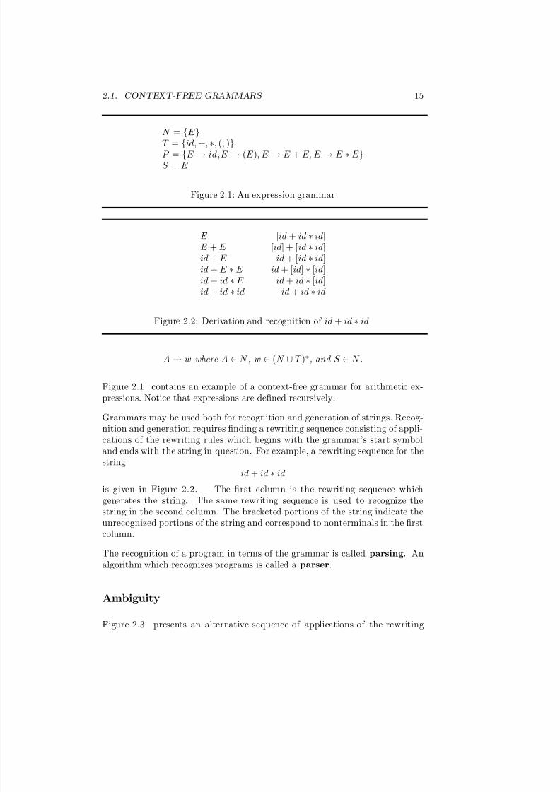
N = {E }T = {id, +, ∗, (, )}P = {E → id,E → (E ), E → E + E, E → E ∗ E }S = E
Figure 2.1: An expression grammar
E [id + id ∗ id]E + E [id] + [id ∗ id]id + E id + [id ∗ id]id + E ∗ E id + [id] ∗ [id]
id + id ∗ E id + id ∗ [id]id + id ∗ id id + id ∗ id
Figure 2.2: Derivation and recognition of id + id ∗ id
A → w where A ∈ N , w ∈ (N ∪ T )∗, and S ∈ N .
Figure 2.1 contains an example of a context-free grammar for arithmetic ex-pressions. Notice that expressions are defined recursively.
Grammars may be used both for recognition and generation of strings. Recog-nition and generation requires finding a rewriting sequence consisting of appli-cations of the rewriting rules which begins with the grammar’s start symboland ends with the string in question. For example, a rewriting sequence for thestring
id + id ∗ id
is given in Figure 2.2. The first column is the rewriting sequence whichgenerates the string. The same rewriting sequence is used to recognize thestring in the second column. The bracketed portions of the string indicate theunrecognized portions of the string and correspond to nonterminals in the firstcolumn.
The recognition of a program in terms of the grammar is called parsing. Analgorithm which recognizes programs is called a parser.
Ambiguity
Figure 2.3 presents an alternative sequence of applications of the rewriting
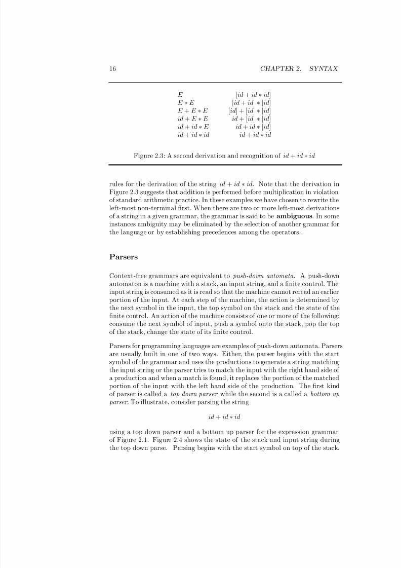
7/3/2019 Theory Introduction to Programming Languages
http://slidepdf.com/reader/full/theory-introduction-to-programming-languages-5584618bb4249 30/233
16 CHAPTER 2. SYNTAX
E [id + id ∗ id]E ∗ E [id + id] ∗ [id]E + E ∗ E [id] + [id] ∗ [id]id + E ∗ E id + [id] ∗ [id]id + id ∗ E id + id ∗ [id]id + id ∗ id id + id ∗ id
Figure 2.3: A second derivation and recognition of id + id ∗ id
rules for the derivation of the string id + id ∗ id. Note that the derivation inFigure 2.3 suggests that addition is performed before multiplication in violation
of standard arithmetic practice. In these examples we have chosen to rewrite theleft-most non-terminal first. When there are two or more left-most derivationsof a string in a given grammar, the grammar is said to be ambiguous. In someinstances ambiguity may be eliminated by the selection of another grammar forthe language or by establishing precedences among the operators.
Parsers
Context-free grammars are equivalent to push-down automata . A push-downautomaton is a machine with a stack, an input string, and a finite control. Theinput string is consumed as it is read so that the machine cannot reread an earlier
portion of the input. At each step of the machine, the action is determined bythe next symbol in the input, the top symbol on the stack and the state of thefinite control. An action of the machine consists of one or more of the following:consume the next symbol of input, push a symbol onto the stack, pop the topof the stack, change the state of its finite control.
Parsers for programming languages are examples of push-down automata. Parsersare usually built in one of two ways. Either, the parser begins with the startsymbol of the grammar and uses the productions to generate a string matchingthe input string or the parser tries to match the input with the right hand side of a production and when a match is found, it replaces the portion of the matchedportion of the input with the left hand side of the production. The first kindof parser is called a top down parser while the second is a called a bottom upparser . To illustrate, consider parsing the string
id + id ∗ id
using a top down parser and a bottom up parser for the expression grammarof Figure 2.1. Figure 2.4 shows the state of the stack and input string duringthe top down parse. Parsing begins with the start symbol on top of the stack.
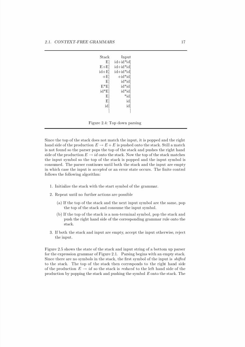
7/3/2019 Theory Introduction to Programming Languages
http://slidepdf.com/reader/full/theory-introduction-to-programming-languages-5584618bb4249 31/233
2.1. CONTEXT-FREE GRAMMARS 17
Stack Input
E] id+id*id]E+E] id+id*id]id+E] id+id*id]
+E] +id*id]E] id*id]
E*E] id*id]id*E] id*id]
E] *id]E] id]id] id]
] ]
Figure 2.4: Top down parsing
Since the top of the stack does not match the input, it is popped and the righthand side of the production E → E + E is pushed onto the stack. Still a matchis not found so the parser pops the top of the stack and pushes the right handside of the production E → id onto the stack. Now the top of the stack matchesthe input symbol so the top of the stack is popped and the input symbol isconsumed. The parser continues until both the stack and the input are emptyin which case the input is accepted or an error state occurs. The finite controlfollows the following algorithm:
1. Initialize the stack with the start symbol of the grammar.
2. Repeat until no further actions are possible
(a) If the top of the stack and the next input symbol are the same, popthe top of the stack and consume the input symbol.
(b) If the top of the stack is a non-terminal symbol, pop the stack andpush the right hand side of the corresponding grammar rule onto thestack.
3. If both the stack and input are empty, accept the input otherwise, rejectthe input.
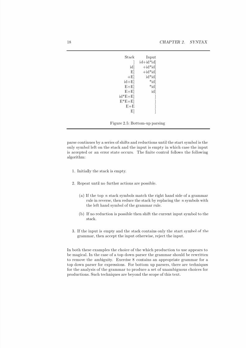
Figure 2.5 shows the state of the stack and input string of a bottom up parserfor the expression grammar of Figure 2.1. Parsing begins with an empty stack.Since there are no symbols in the stack, the first symbol of the input is shifted to the stack. The top of the stack then corresponds to the right hand sideof the production E → id so the stack is reduced to the left hand side of theproduction by popping the stack and pushing the symbol E onto the stack. The
7/3/2019 Theory Introduction to Programming Languages
http://slidepdf.com/reader/full/theory-introduction-to-programming-languages-5584618bb4249 32/233
18 CHAPTER 2. SYNTAX
Stack Input
] id+id*id]id] +id*id]E] +id*id]
+E] id*id]id+E] *id]E+E] *id]E+E] id]
id*E+E] ]E*E+E] ]
E+E ]E] ]
Figure 2.5: Bottom-up parsing
parse continues by a series of shifts and reductions until the start symbol is theonly symbol left on the stack and the input is empty in which case the inputis accepted or an error state occurs. The finite control follows the followingalgorithm:
1. Initially the stack is empty.
2. Repeat until no further actions are possible.
(a) If the top n stack symbols match the right hand side of a grammarrule in reverse, then reduce the stack by replacing the n symbols withthe left hand symbol of the grammar rule.
(b) If no reduction is possible then shift the current input symbol to thestack.
3. If the input is empty and the stack contains only the start symbol of thegrammar, then accept the input otherwise, reject the input.
In both these examples the choice of the which production to use appears tobe magical. In the case of a top down parser the grammar should be rewrittento remove the ambiguity. Exercise 8 contains an appropriate grammar for atop down parser for expressions. For bottom up parsers, there are techniquesfor the analysis of the grammar to produce a set of unambiguous choices forproductions. Such techniques are beyond the scope of this text.
7/3/2019 Theory Introduction to Programming Languages
http://slidepdf.com/reader/full/theory-introduction-to-programming-languages-5584618bb4249 33/233
2.1. CONTEXT-FREE GRAMMARS 19
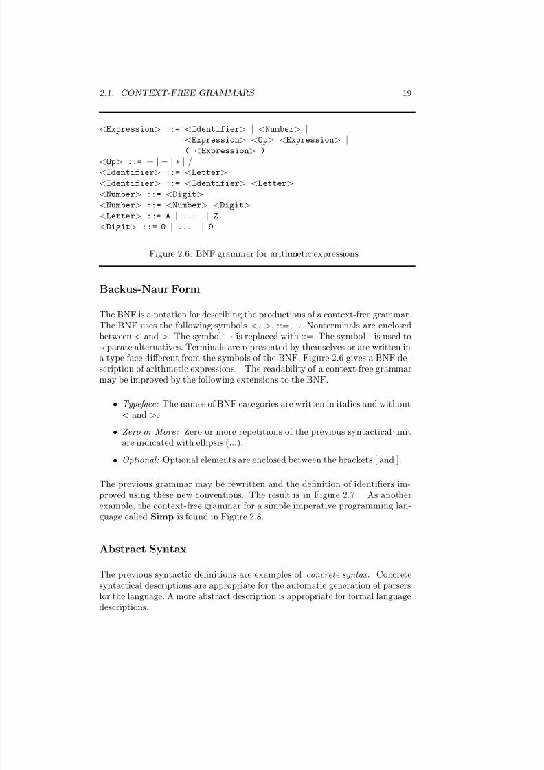
<Expression> ::= <Identifier> | <Number> |<Expression> <Op> <Expression> |( <Expression> )
<Op> ::= + | − | ∗ | /<Identifier> ::= <Letter><Identifier> ::= <Identifier> <Letter><Number> ::= <Digit><Number> ::= <Number> <Digit><Letter> ::= A | ... | Z
<Digit> ::= 0 | ... | 9
Figure 2.6: BNF grammar for arithmetic expressions
Backus-Naur Form
The BNF is a notation for describing the productions of a context-free grammar.The BNF uses the following symbols <, >, ::=, |. Nonterminals are enclosedbetween < and >. The symbol → is replaced with ::=. The symbol | is used toseparate alternatives. Terminals are represented by themselves or are written ina type face different from the symbols of the BNF. Figure 2.6 gives a BNF de-scription of arithmetic expressions. The readability of a context-free grammarmay be improved by the following extensions to the BNF.
• Typeface: The names of BNF categories are written in italics and without< and >.
• Zero or More: Zero or more repetitions of the previous syntactical unitare indicated with ellipsis (...).
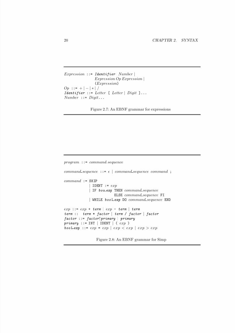
• Optional: Optional elements are enclosed between the brackets [ and ].
The previous grammar may be rewritten and the definition of identifiers im-proved using these new conventions. The result is in Figure 2.7. As anotherexample, the context-free grammar for a simple imperative programming lan-guage called Simp is found in Figure 2.8.
Abstract Syntax
The previous syntactic definitions are examples of concrete syntax . Concretesyntactical descriptions are appropriate for the automatic generation of parsersfor the language. A more abstract description is appropriate for formal languagedescriptions.
7/3/2019 Theory Introduction to Programming Languages
http://slidepdf.com/reader/full/theory-introduction-to-programming-languages-5584618bb4249 34/233
20 CHAPTER 2. SYNTAX
Expression ::= Identifier | Number |Expression Op Expression |(Expression)
Op ::= + | − | ∗ | /Identifier ::= Letter [ Letter | Digit ]...
Number ::= Digit...
Figure 2.7: An EBNF grammar for expressions
program ::= command sequence
command sequence ::= | command sequence command ;
command := SKIP
| IDENT := exp| IF boo exp THEN command sequence
ELSE command sequence FI
| WHILE bool exp DO command sequence END
exp ::= exp + term | exp - term | term
term :: term * factor | term / factor | factor
factor ::= factor ↑primary | primary
primary ::= INT | IDENT | ( exp )
bool exp ::= exp = exp | exp < exp | exp > exp
Figure 2.8: An EBNF grammar for Simp
7/3/2019 Theory Introduction to Programming Languages
http://slidepdf.com/reader/full/theory-introduction-to-programming-languages-5584618bb4249 35/233
2.2. REGULAR EXPRESSIONS 21
program ::= command ...
command ::= SKIP | assignment | conditional | while
assignment ::= IDENT expconditional ::= exp then branch else branch
while ::= exp body
then branch ::= command ...
else branch ::= command ...
body ::= command ...
exp ::= INT | IDENT | exp OP exp
Figure 2.9: An abstract grammar for Simp
Definition 2.6 An abstract syntax for a language consists of a set of syntacticdomains and a set of BNF rules describing the abstract structure.
The idea is to use only as much concrete notation as is necessary to convey thestructure of the objects under description. An abstract syntax for Simp is givenin Figure 2.9. A fully abstract syntax simply gives the components of eachlanguage construct, leaving out the representation details. In the remainder of
the text we will use the term abstract syntax whenever some syntactic detailsare left out.
2.2 Regular Expressions
The lexical units (tokens) of programming languages are defined using regularexpressions. Regular expression describe how characters are grouped to formtokens. The alphabet consists of the character set chosen for the language.
Definition 2.7 Let Σ be an alphabet. The regular expressions over Σ and the
languages (sets of strings) that they denote are defined as follows:
1. ∅ is a regular expression and denotes the empty set. This language containsno strings.
2. is a regular expression and denotes the set {}. This language containsone string, the empty string.
7/3/2019 Theory Introduction to Programming Languages
http://slidepdf.com/reader/full/theory-introduction-to-programming-languages-5584618bb4249 36/233
22 CHAPTER 2. SYNTAX
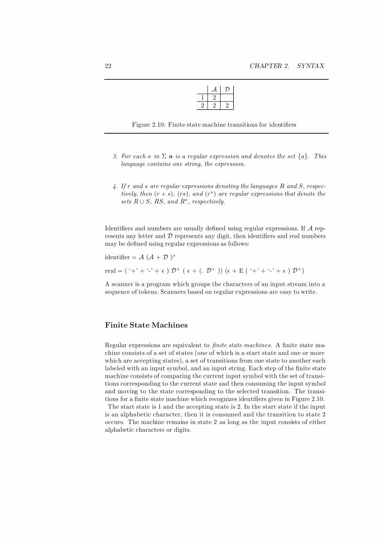
A D
1 22 2 2
Figure 2.10: Finite state machine transitions for identifiers
3. For each a in Σ a is a regular expression and denotes the set {a}. Thislanguage contains one string, the expression.
4. If r and s are regular expressions denoting the languages R and S , respec-tively, then (r + s), (rs), and (r∗) are regular expressions that denote thesets R ∪ S , RS , and R∗, respectively.
Identifiers and numbers are usually defined using regular expressions. If A rep-resents any letter and D represents any digit, then identifiers and real numbersmay be defined using regular expressions as follows:
identifier = A (A + D )∗
real = ( ‘+’ + ‘-’ + ) D+ ( + (. D+ )) ( + E ( ‘+’ + ‘-’ + ) D+)
A scanner is a program which groups the characters of an input stream into asequence of tokens. Scanners based on regular expressions are easy to write.
Finite State Machines
Regular expressions are equivalent to finite state machines. A finite state ma-chine consists of a set of states (one of which is a start state and one or morewhich are accepting states), a set of transitions from one state to another eachlabeled with an input symbol, and an input string. Each step of the finite statemachine consists of comparing the current input symbol with the set of transi-
tions corresponding to the current state and then consuming the input symboland moving to the state corresponding to the selected transition. The transi-tions for a finite state machine which recognizes identifiers given in Figure 2.10.
The start state is 1 and the accepting state is 2. In the start state if the inputis an alphabetic character, then it is consumed and the transition to state 2occurs. The machine remains in state 2 as long as the input consists of eitheralphabetic characters or digits.

7/3/2019 Theory Introduction to Programming Languages
http://slidepdf.com/reader/full/theory-introduction-to-programming-languages-5584618bb4249 37/233
2.3. ATTRIBUTE GRAMMARS AND STATIC SEMANTICS 23
2.3 Attribute Grammars and Static Semantics
Context-free grammars are not able to completely specify the structure of pro-gramming languages. For example, declaration of names before reference, num-ber and type of parameters in procedures and functions, the correspondencebetween formal and actual parameters, name or structural equivalence, scoperules, and the distinction between identifiers and reserved words are all struc-tural aspects of programming languages which cannot be specified using context-free grammars. These context-sensitive aspects of the grammar are often calledthe static semantics of the language. The term dynamic semantics is used torefer to semantics proper, that is, the relationship between the syntax and thecomputational model. Even in a simple language like Simp, context-free gram-mars are unable to specify that variables appearing in expressions must have
an assigned value. Context-free descriptions of syntax are supplemented withnatural language descriptions of the static semantics or are extended to becomeattribute grammars.
Attribute grammars are an extension of context-free grammars which permitthe specification of context-sensitive properties of programming languages. At-tribute grammars are actually much more powerful and are fully capable of specifying the semantics of programming languages as well.
For an example, the following partial syntax of an imperative programminglanguage requires the declaration of variables before reference to the variables.
P ::= D BD ::= V...B ::= C ...C ::= V := E | ...
However, this context-free syntax does not indicate this restriction. The dec-larations define an environment in which the body of the program executes.Attribute grammars permit the explicit description of the environment and itsinteraction with the body of the program.
Since there is no generally accepted notation for attribute grammars, attribute
grammars will be represented as context-free grammars which permit the param-eterization of non-terminals and the addition of where statements which providefurther restrictions on the parameters. Figure 2.3 is an attribute grammar fordeclarations. The parameters marked with ↓ are called inherited attributes anddenote attributes which are passed down the parse tree while the parametersmarked with ↑ are called synthesized attributes and denote attributes which arepassed up the parse tree.

7/3/2019 Theory Introduction to Programming Languages
http://slidepdf.com/reader/full/theory-introduction-to-programming-languages-5584618bb4249 38/233
24 CHAPTER 2. SYNTAX
P ::= D(Env↑) B(Env↓)D(Env↑) ::= ...Vi(Envi−1 ↓,Envi ↑)...
where Env0 = ∅, Env = Envn andEnvi = Envi−1 ∪ {Vi}
B(Env↓) ::= C(Env↓)...C(Env↓) ::= V := E(Env↓) | ...
where V ∈ Env
Figure 2.11: An attribute grammar for declarations
Attribute grammars have considerable expressive power beyond there use tospecify context sensitive portions of the syntax and may be used to specify:
• context sensitive rules
• evaluation of expressions
• translation
2.4 Further Reading
For regular expressions and their relationship to finite automata and context-free grammars and their relationship to push-down automata see texts on formallanguages and automata such as[14]. The original paper on attribute grammarswas by Knuth[15]. For a more recent source and their use in compiler construc-tion and compiler generators see [8, 23]
7/3/2019 Theory Introduction to Programming Languages
http://slidepdf.com/reader/full/theory-introduction-to-programming-languages-5584618bb4249 39/233
2.5. EXERCISES 25
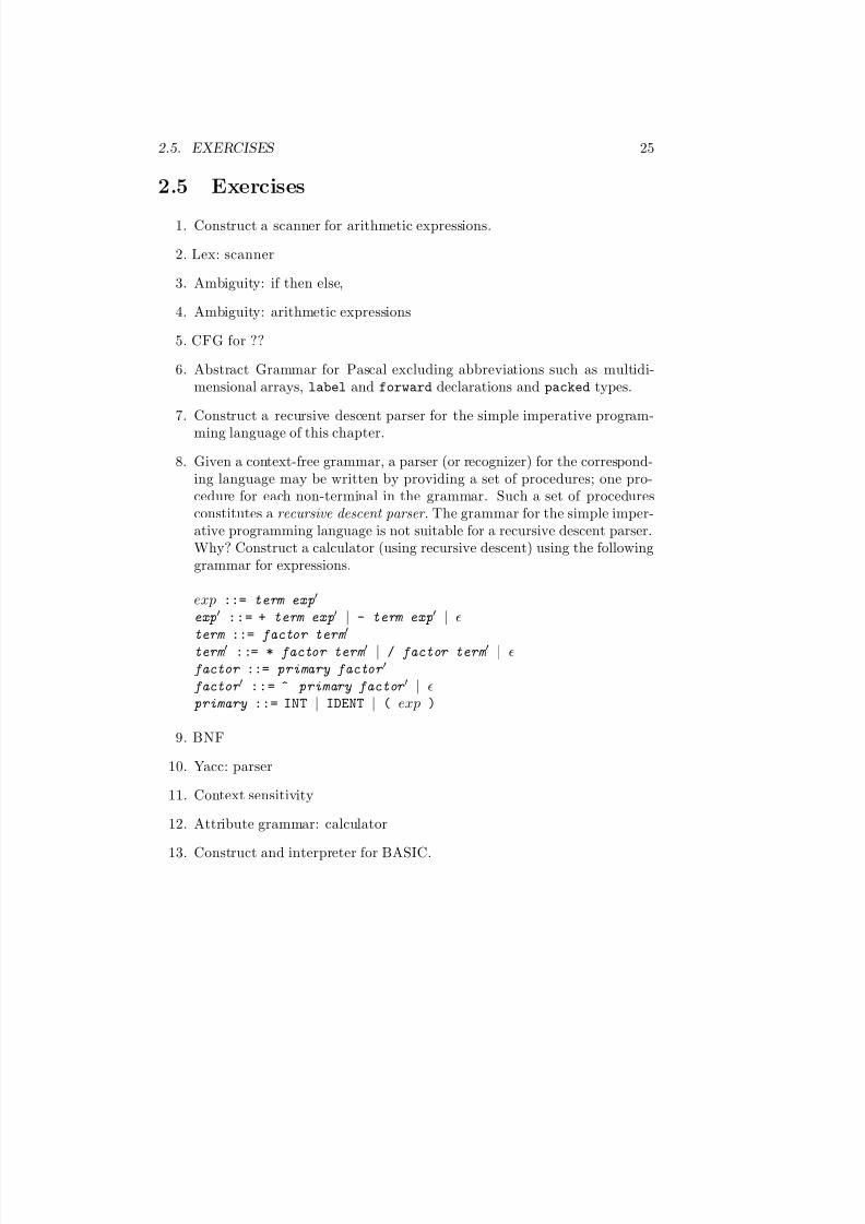
2.5 Exercises
1. Construct a scanner for arithmetic expressions.
2. Lex: scanner
3. Ambiguity: if then else,
4. Ambiguity: arithmetic expressions
5. CFG for ??
6. Abstract Grammar for Pascal excluding abbreviations such as multidi-mensional arrays, label and forward declarations and packed types.
7. Construct a recursive descent parser for the simple imperative program-
ming language of this chapter.
8. Given a context-free grammar, a parser (or recognizer) for the correspond-ing language may be written by providing a set of procedures; one pro-cedure for each non-terminal in the grammar. Such a set of proceduresconstitutes a recursive descent parser . The grammar for the simple imper-ative programming language is not suitable for a recursive descent parser.Why? Construct a calculator (using recursive descent) using the followinggrammar for expressions.
exp ::= term exp
exp ::= + term exp | - term exp | term ::= factor term
term ::= * factor term | / factor term | factor ::= primary factor
factor ::= ^ primary factor | primary ::= INT | IDENT | ( exp )
9. BNF
10. Yacc: parser
11. Context sensitivity
12. Attribute grammar: calculator
13. Construct and interpreter for BASIC.

7/3/2019 Theory Introduction to Programming Languages
http://slidepdf.com/reader/full/theory-introduction-to-programming-languages-5584618bb4249 40/233
26 CHAPTER 2. SYNTAX
7/3/2019 Theory Introduction to Programming Languages
http://slidepdf.com/reader/full/theory-introduction-to-programming-languages-5584618bb4249 41/233
Chapter 3
Semantics
The semantics of a programming language describe the relationship between thesyntactical elements and the model of computation.
Keywords and phrases: Algebraic semantics, axiomatic semantics, denotationalsemantics, operational semantics, semantic algebra, semantic axiom, semanticdomain, semantic equation, semantic function, loop variant, loop invariant, val-uation function, sort, signature, many-sorted algebra
Semantics is concerned with the interpretation or understanding of programsand how to predict the outcome of program execution. The semantics of a pro-gramming language describe the relation between the syntax and the model of computation. Semantics can be thought of as a function which maps syntacticalconstructs to the computational model.
semantics : syntax → computational model
This approach is called syntax-directed semantics.
There are four widely used techniques ( algebraic, axiomatic, denotational, andoperational) for the description of the semantics of programming languages.Algebraic semantics describe the meaning of a program by defining an algebrawhich defines algebraic relationships that exist among the language’s syntac-tic elements. The relationships are described by axioms. Axiomatic semanticsmethod does not give the meaning of the program explicitly. Instead, proper-
27
7/3/2019 Theory Introduction to Programming Languages
http://slidepdf.com/reader/full/theory-introduction-to-programming-languages-5584618bb4249 42/233
28 CHAPTER 3. SEMANTICS
ties about language constructs are defined. The properties are expressed withaxioms and inference rules. A property about a program is deduced by usingthe axioms and inference rules. Each program has a pre-condition which de-scribes the initial conditions required by the program prior to execution and apost-condition which describes, upon termination of the program, the desiredprogram property. Denotational semantics tell what is computed by giving amathematical object (typically a function) which is the meaning of the program.Operational semantics tell how a computation is performed by defining how tosimulate the execution of the program. Operational semantics may describethe syntactic transformations which mimic the execution of the program on anabstract machine or define a translation of the program into recursive functions.
Much of the work in the semantics of programming languages is motivated bythe problems encountered in trying to construct and understand imperative
programs—programs with assignment commands. Since the assignment com-mand reassigns values to variables, the assignment can have unexpected effectsin distant portions of the program.
3.1 Algebraic Semantics
An algebraic definition of a language is a definition of an algebra. An algebraconsists of a domain of values and a set of operations (functions) defined on thedomain.
Algebra = < set of values; operations >
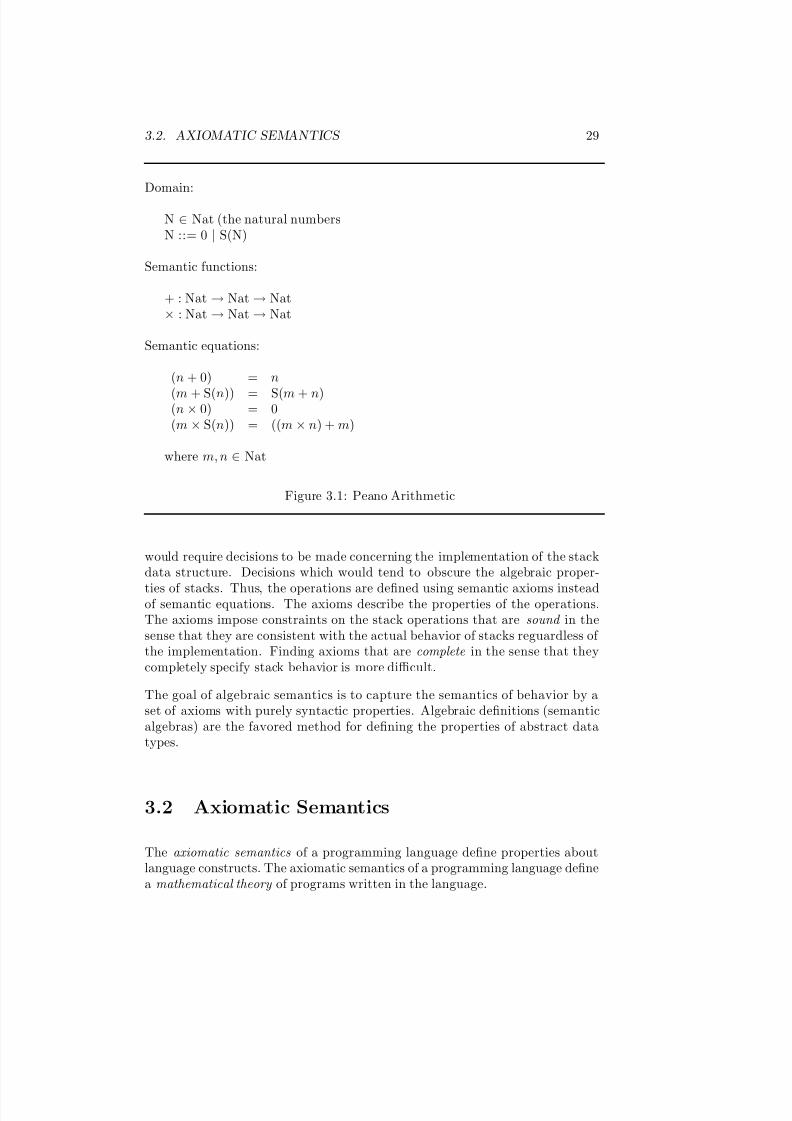
Figure 3.1 is an example of an algebraic definition. It is an algebraic definitionof a fragment of Peano arithmetic. The semantic equations define equivalencesbetween syntactic elements. The equations specify the transformations that areused to translate from one syntactic form to another.
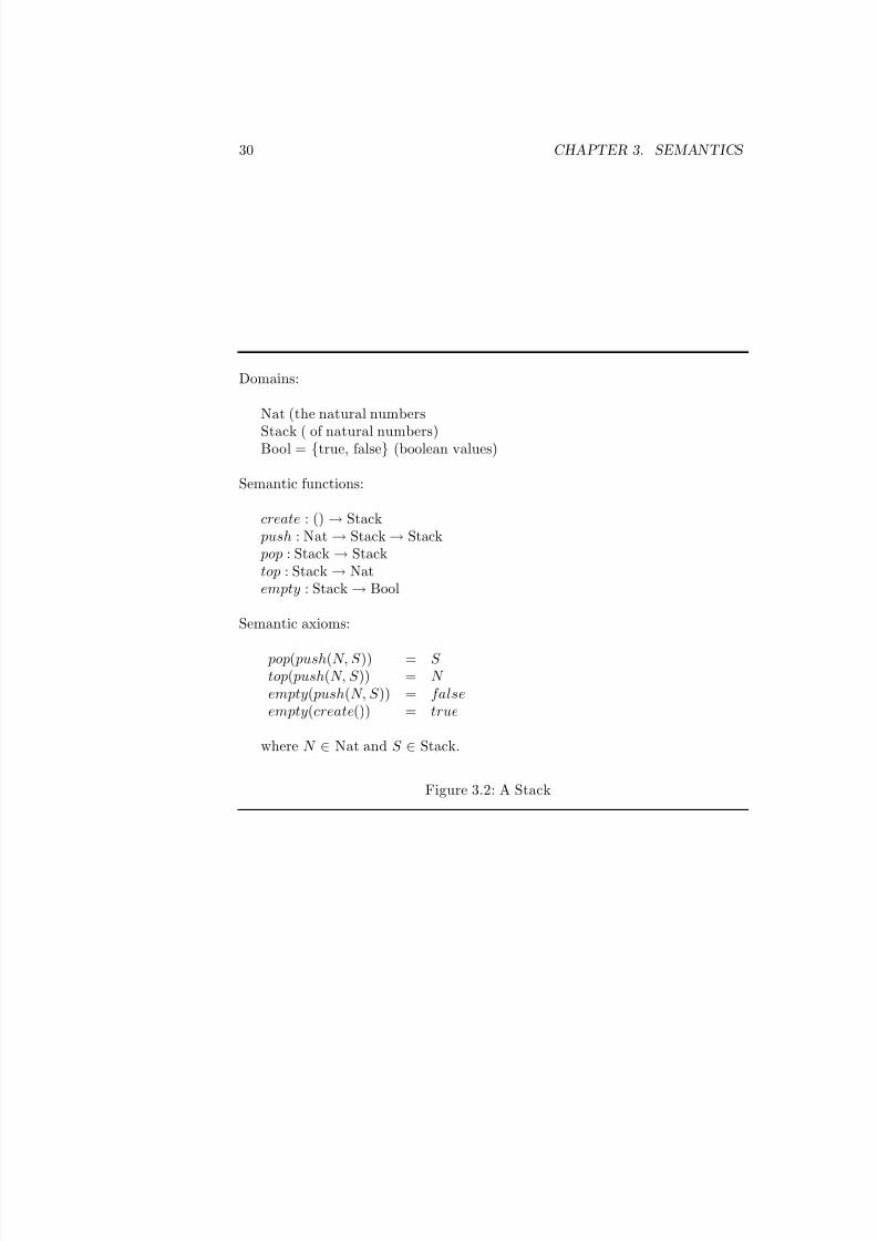
The domain is often called a sort and the domain and the semantic functionsections constitute the signature of the algebra. Functions with zero, one, andtwo operands are referred to as nullary, unary, and binary operations. Oftenabstract data types require values from several different sorts. Such a type ismodeled using a many-sorted algebra. The signature of such an algebra is aset of sorts and a set of functions taking arguments and returning values of different sorts. For example, a stack may be modeled as a many-sorted algebrawith three sorts and four operations. An algebraic definition of a stack is foundin figure 3.2.
The stack example is more abstract than the previous one because the resultsof the operations are not described. This is necessary because the syntacticstructure of the natural numbers and lists are not specified. To be more specific
7/3/2019 Theory Introduction to Programming Languages
http://slidepdf.com/reader/full/theory-introduction-to-programming-languages-5584618bb4249 43/233
3.2. AXIOMATIC SEMANTICS 29
Domain:
N ∈ Nat (the natural numbersN ::= 0 | S(N)
Semantic functions:
+ : Nat → Nat → Nat× : Nat → Nat → Nat
Semantic equations:
(n + 0) = n
(m + S(n)) = S(m + n)(n × 0) = 0(m × S(n)) = ((m × n) + m)
where m, n ∈ Nat
Figure 3.1: Peano Arithmetic
would require decisions to be made concerning the implementation of the stackdata structure. Decisions which would tend to obscure the algebraic proper-
ties of stacks. Thus, the operations are defined using semantic axioms insteadof semantic equations. The axioms describe the properties of the operations.The axioms impose constraints on the stack operations that are sound in thesense that they are consistent with the actual behavior of stacks reguardless of the implementation. Finding axioms that are complete in the sense that theycompletely specify stack behavior is more difficult.
The goal of algebraic semantics is to capture the semantics of behavior by aset of axioms with purely syntactic properties. Algebraic definitions (semanticalgebras) are the favored method for defining the properties of abstract datatypes.
3.2 Axiomatic Semantics
The axiomatic semantics of a programming language define properties aboutlanguage constructs. The axiomatic semantics of a programming language definea mathematical theory of programs written in the language.
7/3/2019 Theory Introduction to Programming Languages
http://slidepdf.com/reader/full/theory-introduction-to-programming-languages-5584618bb4249 44/233
30 CHAPTER 3. SEMANTICS
Domains:
Nat (the natural numbers
Stack ( of natural numbers)Bool = {true, false} (boolean values)
Semantic functions:
create : () → Stack push : Nat → Stack → Stack pop : Stack → Stacktop : Stack → Natempty : Stack → Bool
Semantic axioms:
pop( push(N, S )) = S top( push(N, S )) = N empty( push(N, S )) = falseempty(create()) = true
where N ∈ Nat and S ∈ Stack.
Figure 3.2: A Stack

7/3/2019 Theory Introduction to Programming Languages
http://slidepdf.com/reader/full/theory-introduction-to-programming-languages-5584618bb4249 45/233
3.2. AXIOMATIC SEMANTICS 31
A mathematical theory has three components.
• Syntactic rules: These determine the structure of formulas which arethe statements of interest.
• Axioms: These are basic theorems which are accepted without proof.
• Inference rules: These are the mechanisms for deducing new theoremsfrom axioms and previously proved theorems.
Formulas are triples of the form:
{P } c {Q}
where c is a command in the programming language, P and Q are assertions or
statements concerning the properties of program objects, which may be true orfalse. P is called a pre-condition and Q is called a post-condition . The pre- andpost-conditions are formulas in some arbitrary logic and are used to summarizethe progress of the computation.
The meaning of {P } c {Q}
is that if c is executed in a state in which assertion P is satisfiedand c terminates, then it terminates in a state in which assertion Qis satisfied.
Figure 3.3 is an example of the use of axiomatic semantics in the verification of programs. The program sums the values stored in an array and the program isdecorated with the assertions which help to verify the correctness of the code.Lines 1 and 11 are the pre- and post-conditions respectively for the program.The pre-condition asserts that the number of elements in the array is greaterthan zero and that the sum of the first zero elements of an array is zero. Thepost-condition asserts that S is sum of the values stored in the array. After thefirst assignment we know that the partial sum is the sum of the first I elementsof the array and that I is less than or equal to the number of elements in thearray.
The only way into the body of the while command is if the number of elementssummed is less than the number of elements in the array. When this is the case,The sum of the first I+1 elements of the array is equal to the sum of the firstI elements plus the I+1st element and I+1 is less than or equal to n. After theassignment in the body of the loop, the loop entry assertion holds once more.Upon termination of the loop, the loop index is equal to n.
To show that the program is correct, we must show that the assertions satisfysome verification scheme. To verify the assignment commands on lines 2 and 7
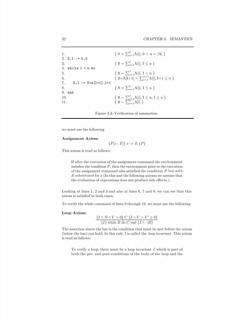
7/3/2019 Theory Introduction to Programming Languages
http://slidepdf.com/reader/full/theory-introduction-to-programming-languages-5584618bb4249 46/233
32 CHAPTER 3. SEMANTICS
1. { 0 = 0
i=1
A[i], 0 < n = |A| }2. S,I := 0,0
3. { S =I
i=1A[i], I ≤ n }4. while I < n do
5. { S =I
i=1A[i], I < n }
6. { S+A[I+1] =I +1
i=1 A[i], I+1 ≤ n }7. S,I := S+A[I+1],I+1
8. { S =I
i=1A[i], I ≤ n }9. end
10. { S =I
i=1A[i], I ≤ n, I ≥ n }11. { S =
ni=1A[i] }
Figure 3.3: Verification of summation
we must use the following
Assignment Axiom:
{P [x : E ]} x := E {P }
This axiom is read as follows:
If after the execution of the assignment command the environmentsatisfies the condition P , then the environment prior to the executionof the assignment command also satisfied the condition P but withE substituted for x (In this and the following axioms we assume thatthe evaluation of expressions does not produce side effects.).
Looking at lines 1, 2 and 3 and also at lines 6, 7 and 8, we can see that thisaxiom is satisfied in both cases.
To verify the while command of lines 3 through 10, we must use the following
Loop Axiom:{I ∧ B ∧ V > 0} C {I ∧ V > V ≥ 0}
{I } while B do C end {I ∧ ¬B}
The assertion above the bar is the condition that must be met before the axiom(below the bar) can hold. In this rule, I is called the loop invariant . This axiomis read as follows:
To verify a loop, there must be a loop invariant I which is part of both the pre- and post-conditions of the body of the loop and the
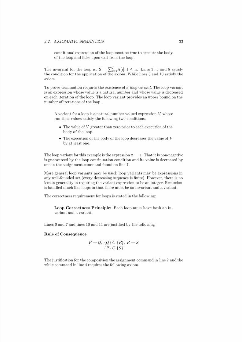
7/3/2019 Theory Introduction to Programming Languages
http://slidepdf.com/reader/full/theory-introduction-to-programming-languages-5584618bb4249 47/233
3.2. AXIOMATIC SEMANTICS 33
conditional expression of the loop must be true to execute the bodyof the loop and false upon exit from the loop.
The invariant for the loop is: S =I
i=1A[i], I ≤ n. Lines 3, 5 and 8 satisfythe condition for the application of the axiom. While lines 3 and 10 satisfy theaxiom.
To prove termination requires the existence of a loop variant . The loop variantis an expression whose value is a natural number and whose value is decreasedon each iteration of the loop. The loop variant provides an upper bound on thenumber of iterations of the loop.
A variant for a loop is a natural number valued expression V whose
run-time values satisfy the following two conditions:
• The value of V greater than zero prior to each execution of thebody of the loop.
• The execution of the body of the loop decreases the value of V by at least one.
The loop variant for this example is the expression n - I. That it is non-negativeis guaranteed by the loop continuation condition and its value is decreased byone in the assignment command found on line 7.
More general loop variants may be used; loop variants may be expressions in
any well-founded set (every decreasing sequence is finite). However, there is noloss in generality in requiring the variant expression to be an integer. Recursionis handled much like loops in that there must be an invariant and a variant.
The correctness requirement for loops is stated in the following:
Loop Correctness Principle: Each loop must have both an in-variant and a variant.
Lines 6 and 7 and lines 10 and 11 are justified by the following
Rule of Consequence:
P → Q, {Q} C {R}, R → S
{P } C {S }
The justification for the composition the assignment command in line 2 and thewhile command in line 4 requires the following axiom.
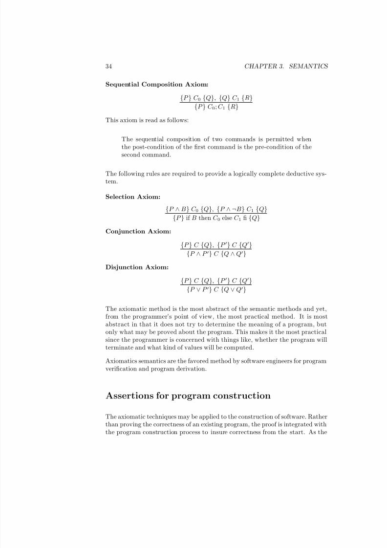
7/3/2019 Theory Introduction to Programming Languages
http://slidepdf.com/reader/full/theory-introduction-to-programming-languages-5584618bb4249 48/233
34 CHAPTER 3. SEMANTICS
Sequential Composition Axiom:
{P } C 0 {Q}, {Q} C 1 {R}{P } C 0; C 1 {R}
This axiom is read as follows:
The sequential composition of two commands is permitted whenthe post-condition of the first command is the pre-condition of thesecond command.
The following rules are required to provide a logically complete deductive sys-tem.
Selection Axiom:
{P ∧ B} C 0 {Q}, {P ∧ ¬B} C 1 {Q}
{P } if B then C 0 else C 1 fi {Q}
Conjunction Axiom:
{P } C {Q}, {P } C {Q}
{P ∧ P } C {Q ∧ Q}
Disjunction Axiom:
{P } C {Q}, {P } C {Q}
{P ∨ P } C {Q ∨ Q}
The axiomatic method is the most abstract of the semantic methods and yet,from the programmer’s point of view, the most practical method. It is mostabstract in that it does not try to determine the meaning of a program, butonly what may be proved about the program. This makes it the most practicalsince the programmer is concerned with things like, whether the program willterminate and what kind of values will be computed.
Axiomatics semantics are the favored method by software engineers for programverification and program derivation.
Assertions for program construction
The axiomatic techniques may be applied to the construction of software. Ratherthan proving the correctness of an existing program, the proof is integrated withthe program construction process to insure correctness from the start. As the
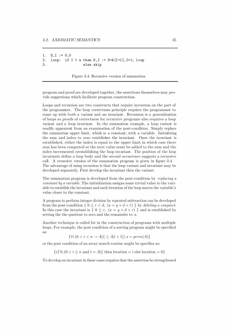
7/3/2019 Theory Introduction to Programming Languages
http://slidepdf.com/reader/full/theory-introduction-to-programming-languages-5584618bb4249 49/233
3.2. AXIOMATIC SEMANTICS 35
1. S,I := 0,0
2. loop: if I < n then S,I := S+A[I+1],I+1; loop
3. else skip
Figure 3.4: Recursive version of summation
program and proof are developed together, the assertions themselves may pro-vide suggestions which facilitate program construction.
Loops and recursion are two constructs that require invention on the part of the programmer. The loop correctness principle requires the programmer to
come up with both a variant and an invariant. Recursion is a generalizationof loops so proofs of correctness for recursive programs also requires a loopvariant and a loop invariant. In the summation example, a loop variant isreadily appearent from an examination of the post-condition. Simply replacethe summation upper limit, which is a constant, with a variable. Initializingthe sum and index to zero establishes the invariant. Once the invariant isestablished, either the index is equal to the upper limit in which case theresum has been computed or the next value must be added to the sum and theindex incremented reestablishing the loop invariant. The position of the loopinvariants define a loop body and the second occurrence suggests a recursivecall. A recursive version of the summation program is given in figure 3.4.The advantage of using recursion is that the loop variant and invariant may bedeveloped separately. First develop the invariant then the variant.
The summation program is developed from the post-condition by replacing a constant by a variable. The initialization assigns some trivial value to the vari-able to establish the invariant and each iteration of the loop moves the variable’svalue closer to the constant.
A program to perform integer division by repeated subtraction can be developedfrom the post-condition { 0 ≤ r < d, (a = q × d + r) } by deleting a conjunct .In this case the invariant is { 0 ≤ r, (a = q × d + r) } and is established bysetting the the quotient to zero and the remainder to a .
Another technique is called for in the construction of programs with multipleloops. For example, the post condition of a sorting program might be specified
as:{∀i.(0 < i < n → A[i] ≤ A[i + 1]), s = perm(A)}
or the post condition of an array search routine might be specifies as:
{if ∃i.(0 < i ≤ n and t = A[i] then location = i else location = 0}
To develop an invariant in these cases requires that the assertion be strengthened
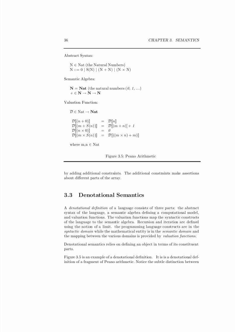
7/3/2019 Theory Introduction to Programming Languages
http://slidepdf.com/reader/full/theory-introduction-to-programming-languages-5584618bb4249 50/233
36 CHAPTER 3. SEMANTICS
Abstract Syntax:
N ∈ Nat (the Natural Numbers)N ::= 0 | S(N) | (N + N) | (N × N)
Semantic Algebra:
N = Nat (the natural numbers (0, 1, ...)+ ∈ N → N → N
Valuation Function:
D ∈ Nat → Nat
D[[(n + 0)]] = D[[n]]D[[(m + S (n))]] = D[[(m + n)]]+ 1D[[(n × 0)]] = 0 D[[(m × S (n))]] = D[[((m × n) + m)]]
where m,n ∈ Nat
Figure 3.5: Peano Arithmetic
by adding additional constraints. The additional constraints make assertionsabout different parts of the array.
3.3 Denotational Semantics
A denotational definition of a language consists of three parts: the abstractsyntax of the language, a semantic algebra defining a computational model,and valuation functions. The valuation functions map the syntactic constructsof the language to the semantic algebra. Recursion and iteration are definedusing the notion of a limit. the programming language constructs are in the
syntactic domain while the mathematical entity is in the semantic domain andthe mapping between the various domains is provided by valuation functions.
Denotational semantics relies on defining an object in terms of its constituentparts.
Figure 3.5 is an example of a denotational definition. It is is a denotational def-inition of a fragment of Peano arithmetic. Notice the subtle distinction between
7/3/2019 Theory Introduction to Programming Languages
http://slidepdf.com/reader/full/theory-introduction-to-programming-languages-5584618bb4249 51/233
3.4. OPERATIONAL SEMANTICS 37
the syntactic and semantic domains. The syntactic expressions are mapped intoan algebra of the natural numbers by the valuation function. The denotationaldefinition almost seem to be unnecessary. Since the syntax so closely resem-bles that of the semantic algebra. Programming languages are not as close totheir computational model. Figure 3.6 is denotational definition of the smallimperative programming language Simp encountered in the previous chapter.
Denotational definitions are favored for theoretical and comparative program-ming language studies. Denotational definitions have been used for the auto-matic construction of compilers for the programming language. Denotationsother than mathematical objects are possible. For example, a compiler writerwould prefer that the object denoted would be appropriate object code. Sys-tems have been developed for the automatic construction of compilers from thedenotation specification of a programming language.
3.4 Operational Semantics
An operational definition of a language consists of two parts: an abstract syn-tax and an interpreter. An interpreter defines how to perform a computation.When the interpreter evaluates a program, it generates a sequence of machineconfigurations that define the program’s operational semantics. The interpreteris an evaluation relation that is defined by rewriting rules. The interpreter maybe an abstract machine or recursive functions.
Figure 3.7 an example of an operational definition. It is is an operationaldefinition of a fragment of Peano arithmetic.
The interpreter is used to rewrite natural number expressions to a standardform (a form involving only S and 0 ) and the rewriting rules show how movethe + and × operators inward toward the base cases. Operational definitionsare favored by language implementors for the construction of compilers and bylanguage tutorials because operational definitions describe how the actions takeplace.
The operational semantics of Simp is found in figure 3.8. The operationalsemantics are defined by using two semantic functions, I which interprets com-mands and ν which evaluates expressions. The interpreter is more complex since
there is an environment associated with the program with does not appear asa syntactic element and the environment is the result of the computation. Theenvironment (variously called the store or referencing environment ) is an associ-ation between variables and the values to which they are assigned. Initially theenvironment is empty since no variable has been assigned to a value. Duringprogram execution each assignment updates the environment. The interpreterhas an auxiliary function which is used to evaluate expressions. The while com-
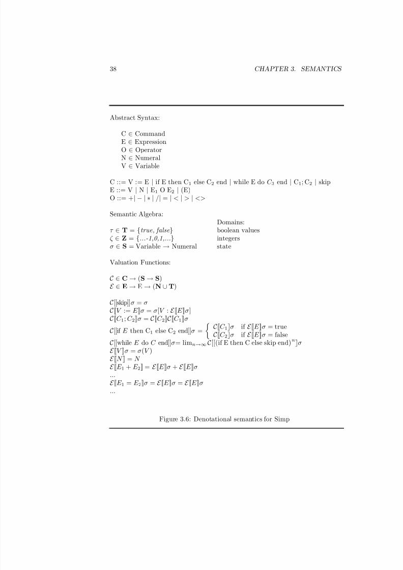
7/3/2019 Theory Introduction to Programming Languages
http://slidepdf.com/reader/full/theory-introduction-to-programming-languages-5584618bb4249 52/233
38 CHAPTER 3. SEMANTICS
Abstract Syntax:
C ∈ CommandE ∈ ExpressionO ∈ OperatorN ∈ NumeralV ∈ Variable
C ::= V := E | if E then C1 else C2 end | while E do C 3 end | C1; C2 | skipE ::= V | N | E1 O E2 | (E)
O ::= +| − | ∗ | /| = | < | > | <>
Semantic Algebra:Domains:
τ ∈ T = {true, false} boolean valuesζ ∈ Z = {...-1,0,1,...} integersσ ∈ S = Variable → Numeral state
Valuation Functions:
C ∈ C → (S → S)E ∈ E → E → (N ∪ T)
C[[skip]]σ = σC[[V := E ]]σ = σ[V : E [[E ]]σ]C[[C 1; C 2]]σ = C[[C 2]]C[[C 1]]σ
C[[if E then C1 else C2 end]]σ =
C[[C 1]]σ if E [[E ]]σ = trueC[[C 2]]σ if E [[E ]]σ = false
C[[while E do C end]]σ= limn→∞ C[[(if E then C else skip end)n]]σE [[V ]]σ = σ(V )E [[N ]] = N E [[E 1 + E 2]] = E [[E ]]σ + E [[E ]]σ...E [[E 1 = E 2]]σ = E [[E ]]σ = E [[E ]]σ...
Figure 3.6: Denotational semantics for Simp
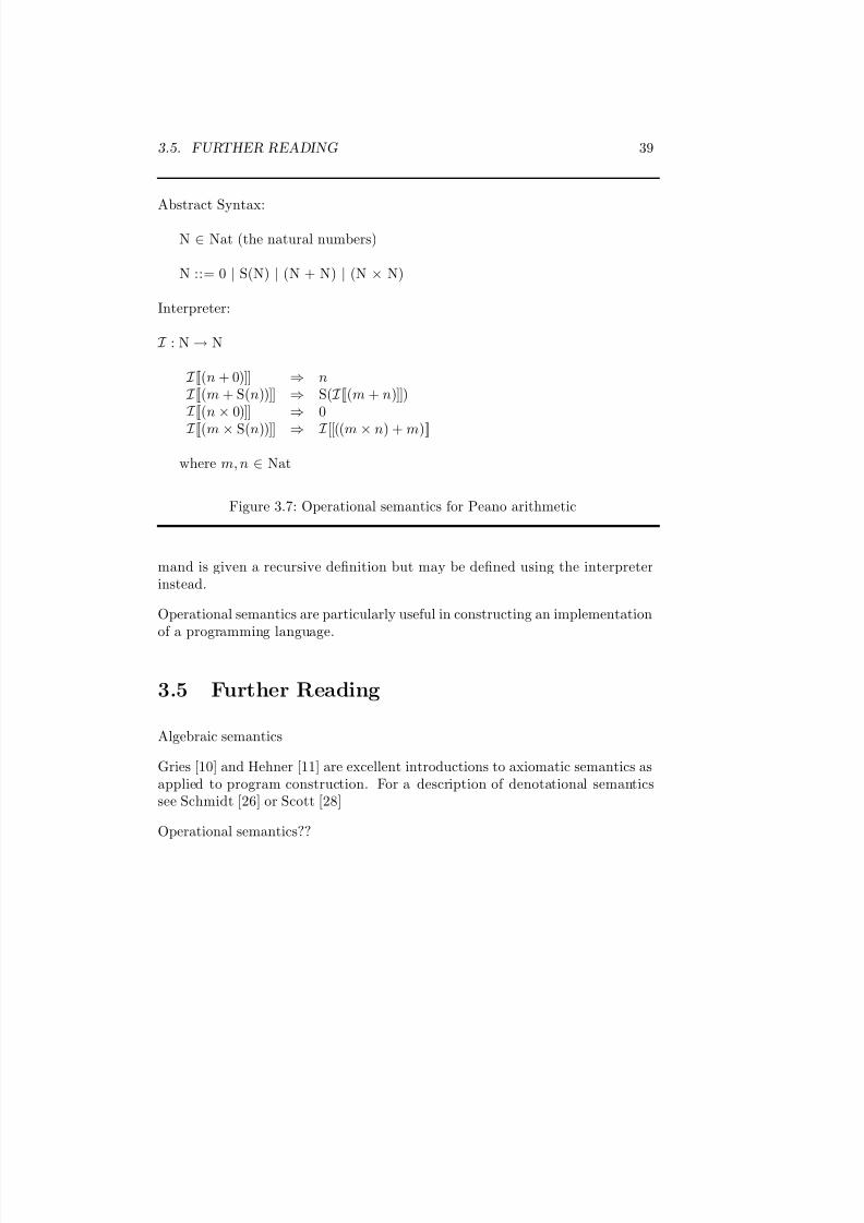
7/3/2019 Theory Introduction to Programming Languages
http://slidepdf.com/reader/full/theory-introduction-to-programming-languages-5584618bb4249 53/233
3.5. FURTHER READING 39
Abstract Syntax:
N ∈ Nat (the natural numbers)
N ::= 0 | S(N) | (N + N) | (N × N)
Interpreter:
I : N → N
I [[(n + 0)]] ⇒ n I [[(m + S(n))]] ⇒ S( I [[(m + n)]]) I [[(n × 0)]] ⇒ 0
I [[(m × S(n))]] ⇒ I [[((m × n) + m)]]
where m, n ∈ Nat
Figure 3.7: Operational semantics for Peano arithmetic
mand is given a recursive definition but may be defined using the interpreterinstead.
Operational semantics are particularly useful in constructing an implementationof a programming language.
3.5 Further Reading
Algebraic semantics
Gries [10] and Hehner [11] are excellent introductions to axiomatic semantics asapplied to program construction. For a description of denotational semanticssee Schmidt [26] or Scott [28]
Operational semantics??
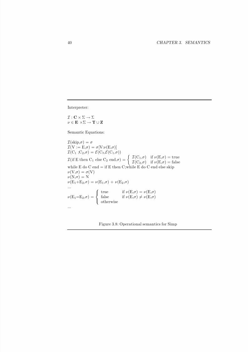
7/3/2019 Theory Introduction to Programming Languages
http://slidepdf.com/reader/full/theory-introduction-to-programming-languages-5584618bb4249 54/233
40 CHAPTER 3. SEMANTICS
Interpreter:
I : C × Σ → Σ
ν ∈ E ×Σ → T ∪ Z
Semantic Equations:
I (skip,σ) = σ I (V := E,σ) = σ[V:ν (E,σ)] I (C1 ;C2,σ) = E (C2,E (C1,σ))
I (if E then C1 else C2 end,σ) =
I (C1,σ) if ν (E,σ) = true
I (C2,σ) if ν (E,σ) = falsewhile E do C end = if E then C;while E do C end else skipν (V,σ) = σ(V)ν (N,σ) = Nν (E1+E2,σ) = ν (E1,σ) + ν (E2,σ)...
ν (E1=E2,σ) =
true if ν (E,σ) = ν (E,σ)false if ν (E,σ) = ν (E,σ)otherwise
...
Figure 3.8: Operational semantics for Simp
7/3/2019 Theory Introduction to Programming Languages
http://slidepdf.com/reader/full/theory-introduction-to-programming-languages-5584618bb4249 55/233
Chapter 4
Abstraction and
Generalization I
Abstraction is an emphasis on the idea, qualities and properties rather than theparticulars (a suppression of detail).
Generalization is a broadening of application to encompass a larger domain of objects of the same or different type.
A parameter is a quantity whose value varies with the circumstances of its
application.Substitution—To put something in the place of another.
Keywords and phrases: Name, binding, abstract, definition, declaration, vari-ables, parameters, arguments, formals, actuals.
The ability to abstract and to generalize is an essential part of any intellec-tual activity. Abstraction and generalization are the basis for mathematics andphilosophy and are essential in computer science as well.
The importance of abstraction is derived from its ability to hide irrelevant de-tails and from the use of names to reference objects. Programming languagesprovide abstraction through procedures, functions, and modules which permit
41
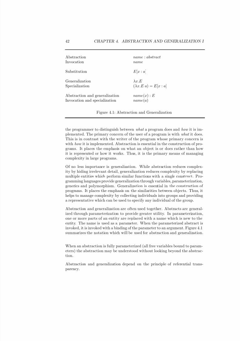
7/3/2019 Theory Introduction to Programming Languages
http://slidepdf.com/reader/full/theory-introduction-to-programming-languages-5584618bb4249 56/233
42 CHAPTER 4. ABSTRACTION AND GENERALIZATION I
Abstraction name : abstractInvocation name
Substitution E [x : a]
Generalization λx.E Specialization (λx.E a) = E [x : a]
Abstraction and generalization name(x) : E Invocation and specialization name(a)
Figure 4.1: Abstraction and Generalization
the programmer to distinguish between what a program does and how it is im-plemented. The primary concern of the user of a program is with what it does.This is in contrast with the writer of the program whose primary concern iswith how it is implemented. Abstraction is essential in the construction of pro-grams. It places the emphasis on what an object is or does rather than howit is represented or how it works. Thus, it is the primary means of managingcomplexity in large programs.
Of no less importance is generalization. While abstraction reduces complex-ity by hiding irrelevant detail, generalization reduces complexity by replacingmultiple entities which perform similar functions with a single construct. Pro-gramming languages provide generalization through variables, parameterization,generics and polymorphism. Generalization is essential in the construction of programs. It places the emphasis on the similarities between objects. Thus, ithelps to manage complexity by collecting individuals into groups and providinga representative which can be used to specify any individual of the group.
Abstraction and generalization are often used together. Abstracts are general-ized through parameterization to provide greater utility. In parameterization,one or more parts of an entity are replaced with a name which is new to theentity. The name is used as a parameter. When the parameterized abstract isinvoked, it is invoked with a binding of the parameter to an argument. Figure 4.1summarizes the notation which will be used for abstraction and generalization.
When an abstraction is fully parameterized (all free variables bound to param-eters) the abstraction may be understood without looking beyond the abstrac-tion.
Abstraction and generalization depend on the principle of referential trans-parency.
7/3/2019 Theory Introduction to Programming Languages
http://slidepdf.com/reader/full/theory-introduction-to-programming-languages-5584618bb4249 57/233
4.1. ABSTRACTION 43
Principle of Referential Transparency: The meaning of an entity is un-changed when a part of the entity is replaced with an equal part.
4.1 Abstraction
Principle of Abstraction: An abstract is a named entity which may be in-voked by mentioning the name.
Giving an object a name gives permission to substitute the name for the thingnamed (or vice versa) without changing the meaning. We use the notation
name : abstract
to denote the binding of a name to an abstract.
Abstraction permits the recognition and elimination of common subexpressionsas in the following example:
(x+y-z)*(x+y-z) =⇒ a*a where a = x+y-z
This example motivates the use of functions and procedures in programminglanguages.
In addition to naming and substitution there is a third aspect to abstraction.It is that the abstract is encapsulated, that is, the details of the abstract are
hidden so that the name is sufficient to represent the entity. This aspect of abstraction is considered in more detail in a later chapter.
An object is said to be fully abstract if it can be understood without referenceto any thing external to the object.
Terminology: The naming aspect of abstraction is captured in the conceptsof binding , definition and declaration while the hiding of irrelevant details iscaptured by the concept of encapsulation. 2
Binding
The concept of binding is common to all programming languages. A binding isan association of two entities. The objects which may be bound to identifiersare called the bindables of the language. The bindables may include: primitivevalues, compound values, references to variables, types, and executable abstrac-tions. While binding occurs in definitions and declarations, it also occurs at thevirtual and hardware machine levels.
7/3/2019 Theory Introduction to Programming Languages
http://slidepdf.com/reader/full/theory-introduction-to-programming-languages-5584618bb4249 58/233
44 CHAPTER 4. ABSTRACTION AND GENERALIZATION I
The imperative programming paradigm is characterized by permitting namesto be bound successively to different objects, this is accomplished by the as-signment statement (often of the form; name := object) which means “let namestand for object until further notice.” In other words, until it is reassigned.This is in contrast with functional and logic programming paradigms in whichnames may not be reassigned. Thus languages in these paradigms are oftencalled single assignment languages.
Terminology: We could equally well say identifier instead of name as in someother texts. Among the various terms for abstracts found in other texts are mod-ule, package, library , unit , subprogram , subroutine, routine, function , procedure,abstract type, object . 2
4.2 Generalization
Principle of Generalization: A generic is an entity which may be elaboratedupon invocation.
Generalization permits the use of a single pattern to represent each member of a group. We use the notation:
λx.B
to denote the generalization of the object B where x is called a parameter andB is the object B with x replacing any number of occurences of some part of B by x . The parameter x is said to be bound in the expression but free in B and
the scope of x is said to be B .
The symbol λ (lambda) is a quantifier . Quantifiers introduce variables intoobjects.
Aside: The symbol λ was introduced by Church for variable introduction inthe lambda calculus. It roughly corrresponds to the symbol ∀, the universalquantifier, of first-order logic. The appendix contains a brief introduction tofirst-order logic. 2
Generalization is often combined with abstraction and takes the following form:
p(x) : B
where p is the name, x is the parameter, and B is the abstract. The invocationof the abstract takes the form:
( p a) or p(a)
where p is the name and a is called the argument whose value (called the ar-gument ) is substituted for the parameter. Upon invocation of the abstract, theargument is bound to the parameter.
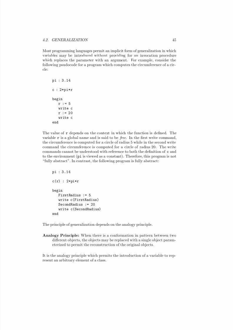
7/3/2019 Theory Introduction to Programming Languages
http://slidepdf.com/reader/full/theory-introduction-to-programming-languages-5584618bb4249 59/233
4.2. GENERALIZATION 45
Most programming languages permit an implicit form of generalization in whichvariables may be introduced without providing for an invocation procedurewhich replaces the parameter with an argument. For example, consider thefollowing psudocode for a program which computes the circumference of a cir-cle:
pi : 3.14
c : 2*pi*r
begin
r : = 5
write c
r := 20
write c
end
The value of r depends on the context in which the function is defined. Thevariable r is a global name and is said to be free. In the first write command,the circumference is computed for a circle of radius 5 while in the second writecommand the circumference is computed for a circle of radius 20. The writecommands cannot be understood with reference to both the definition of c andto the environment (pi is viewed as a constant). Therefore, this program is not“fully abstract”. In contrast, the following program is fully abstract:
pi : 3.14
c(r) : 2*pi*r
begin
FirstRadius := 5
write c(FirstRadius)
SecondRadius := 20
write c(SecondRadius)
end
The principle of generalization depends on the analogy principle.
Analogy Principle: When there is a conformation in pattern between twodifferent objects, the objects may be replaced with a single object param-eterized to permit the reconstruction of the original objects.
It is the analogy principle which permits the introduction of a variable to rep-resent an arbitrary element of a class.
7/3/2019 Theory Introduction to Programming Languages
http://slidepdf.com/reader/full/theory-introduction-to-programming-languages-5584618bb4249 60/233
46 CHAPTER 4. ABSTRACTION AND GENERALIZATION I
The Principle of Generalization makes no restrctions on parameters or the partsof an entity that may be parameterized. Neither should programming lanauges.This is emphasized in the following principle:
Principle of Parameterization: A parameter of a generic may be from anydomain.
Terminology: The terms formal parameters ( formals) and actual parameters(actuals) are sometimes used instead of the terms parameters and argumentsrespectively. 2
4.3 Substitution
The utility of both abstraction and generalization depend on substitution. Thetie between the two is captured in the following principle:
Principle of Correspondence: Parameter binding mechanisms and defini-tion mechanisms are equivalent.
The Principle of Correspondence is a formalization of that aspect of the Prin-ciple of Abstraction that implies that definition and substitution are intimatelyrelated.
We use the notation E [x : a]
to denote the substitution of a for x in E . The notation is read as “E [x : a] isthe expression obtained from E by replacing all occurrences of x with a.”
Terminology: The notation for substitution was chosen to emphasize the re-lationship between abstraction and substitution. Other texts use the notationE [a/x] for substitution. That notation is motivated by the cancelation thatoccurs when a number is multiplied by its inverse ( x(a/x) = a). 2
4.4 Abstraction and Generalization
Together, abstraction and generalization provide a powerful mechanism for pro-gram development. Generalization provides a mechanism for the constructionof common subexpressions and abstraction a mechanism for the factoring outof the common subexpressions. In the following example, the factors are firstgeneralized to contain common subexpressions and then abstracted out.
7/3/2019 Theory Introduction to Programming Languages
http://slidepdf.com/reader/full/theory-introduction-to-programming-languages-5584618bb4249 61/233
4.5. EXERCISES 47
(a+b-c)*(x+y-z) =⇒ (λ i j k. i+j-k) a b c * (λ i j k. i+j-k) x y z=⇒ f a b c * f x y z where f i j k = i+j-k
4.5 Exercises
1. Extend the compiler to handle constant, type, variable, function and pro-cedure definitions and references to the same.
2. What is the effect of providing lazy evaluation in an imperative program-ming language?
3. Extend the compiler to handle parameterization of functions and proce-dures.
4. For a specific programming language, report on its provision for abstrac-tion and generalization. Specifically, what entities may be named, whatentities may be parameterized, what entities may be passed as parame-ters, and what entities may be returned as results (of functions). Whatirregularities do you find in the language?

7/3/2019 Theory Introduction to Programming Languages
http://slidepdf.com/reader/full/theory-introduction-to-programming-languages-5584618bb4249 62/233
48 CHAPTER 4. ABSTRACTION AND GENERALIZATION I

7/3/2019 Theory Introduction to Programming Languages
http://slidepdf.com/reader/full/theory-introduction-to-programming-languages-5584618bb4249 63/233
Chapter 5
Domains and Types
A value is any thing that may be evaluated, stored, incorporated in a data struc-ture, passed as an argument or returned as a result.
What is a type?
Realist: A type is a set of values.
Idealist: No. A type is a conceptual entity whose values are accessible only through the interpretive filter of type.
Beginning Programmer: Isn’t a type a name for a set of values?
Intermediate Programmer: No. A type is a way to classify values by their properties and behavior.
Advanced Programmer: No. A type is a set of values and operations.
Algebraist: Ah! So a type is an algebra, a set of values and operations defined on the values.
Type checker: Types are more practical than that, they are constraints on expressions to ensure compatibility between operators and their operand(s).
Type Inference System: Yes and more, since a type system is a set of rules for associating with every expression a unique and most general type that reflects the set of all meaningful contexts in which the expression may occur.
Program verifier: Lets keep it simple, types are the behavioral invariants that instances of the type must satisfy.
49

7/3/2019 Theory Introduction to Programming Languages
http://slidepdf.com/reader/full/theory-introduction-to-programming-languages-5584618bb4249 64/233
50 CHAPTER 5. DOMAINS AND TYPES
Software engineer: What is important to me is that types are a tool for man-aging software development and evolution.
Compiler: All this talk confuses me, types specify the storage requirements for variables of the type.
7/3/2019 Theory Introduction to Programming Languages
http://slidepdf.com/reader/full/theory-introduction-to-programming-languages-5584618bb4249 65/233
51
Keywords and phrases: value, domain, type, type constructor, Cartesian prod-uct, disjoint union, map, power set, recursive type, binding, strong and weaktyping, static and dynamic type checking, type inference, type equivalence, nameand structural equivalence, abstract types, generic types.
A computation is a sequence of operations applied to a value to yield a value.Thus values and operations are fundamental to computation. Values are thesubject of this chapter and operations are the subject of later chapters.
In mathematical terminology, the sets from which the arguments and results of a function are taken are known as the function’s “domain” and “codomain”,
respectively. Consequently, the term domain will denote any set of values thatcan be passed as arguments or returned as results. Associated with every domainare certain “essential” operations. For example, the domain of natural numbersis equipped with an the “constant” operation which produces the number zeroand the operation that constructs the successor of any number. Additionaloperations (such as addition and multiplication) on the natural numbers maybe defined using these basic operations.
Programming languages utilize a rich set of domains. Truth values, charac-ters, integers, reals, records, arrays, sets, files, pointers, procedure and functionabstractions, environments, commands, and definitions are but some of the do-mains that are found in programming languages. There are two approachesto domains. One approach is to assume the existence of a universal domain.
It contains all those objects which are of computational interest. The secondapproach is to begin with a small set of values and some rules for combining thevalues and then to construct the universe of values. Programming languagesfollow the second approach by providing several basic sets of values and a set of domain constructors from which additional domains may be constructed.
Domains are categorized as primitive or compound . A primitive domain is a setthat is fundamental to the application being studied. Its elements are atomic.A compound domain is a set whose values are constructed from existing domainsby one or more domain constructors.
Aside: It is common in mathematics to define a set but fail to give an effectivemethod for determining membership in the set. Computer science on the other
hand is concerned with determining membership with in a finite number of steps. In addition, a program is often constrained by requirements to completeits work with in bounds of time and space. 2
Terminology: Domain theory is the study of structured sets and theiroperations. A domain is a set of elements and an accompanying set of operations defined on the domain.
7/3/2019 Theory Introduction to Programming Languages
http://slidepdf.com/reader/full/theory-introduction-to-programming-languages-5584618bb4249 66/233
52 CHAPTER 5. DOMAINS AND TYPES
The terms domain , type, and data type may be used interchangeably.
The term data refers to either an element of a domain or a collection of elements from one or more domains.
The terms compound, composite and structured when applied to values, data,domains, types are used interchangeably. 2
5.1 Primitive Domains
Among the primitive types provided by programming languages are
Truth-value = { false, true}Integer = {..., -2, -1, 0, +1, +2, ...}Real = {..., -1.0, ..., 0.0, ..., +1.0, ...}Character = {..., a, b, ..., z, ...}
The values are represented as a particular pattern of bits in the storage of thecomputer.
Aside: Programming language definitions do not place restrictions on theprimitive types. However hardware limitations and variation have considerableinfluence on actual programs so that, Integer is an implementation defined rangeof whole numbers, Real is an implementation defined subset of the rational
numbers and Character is an implementation defined set of characters.2
Several languages permit the user to define additional primitive types. Theseprimitive types are called enumeration types.
5.2 Compound Domains
There are many compound domains that are useful in computer science: arrays,tuples, records, variants, unions, sets, lists, trees, files, relations, definitions,mappings, etc, are all examples of compound domains. Each of these domainsmay be constructed from simpler domains by one or more applications of domain
constructors.
Compound domains are constructed by a domain builder. A domain builderconsists of a set of operations for assembling and disassembling elements of acompound domain. The domain builders are:
• Product Domains
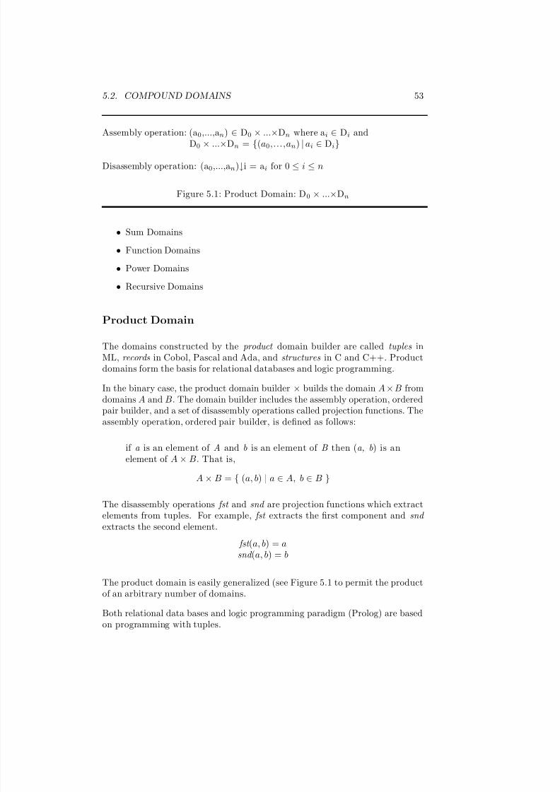
7/3/2019 Theory Introduction to Programming Languages
http://slidepdf.com/reader/full/theory-introduction-to-programming-languages-5584618bb4249 67/233
5.2. COMPOUND DOMAINS 53
Assembly operation: (a0,...,an) ∈ D0 × ...×Dn where ai ∈ Di andD0 × ...×Dn = {(a0,...,an) | ai ∈ Di}
Disassembly operation: (a0,...,an)↓i = ai for 0 ≤ i ≤ n
Figure 5.1: Product Domain: D0 × ...×Dn
• Sum Domains
• Function Domains
• Power Domains
• Recursive Domains
Product Domain
The domains constructed by the product domain builder are called tuples inML, records in Cobol, Pascal and Ada, and structures in C and C++. Productdomains form the basis for relational databases and logic programming.
In the binary case, the product domain builder × builds the domain A × B fromdomains A and B. The domain builder includes the assembly operation, orderedpair builder, and a set of disassembly operations called projection functions. Theassembly operation, ordered pair builder, is defined as follows:
if a is an element of A and b is an element of B then (a, b) is anelement of A × B. That is,
A × B = { (a, b) | a ∈ A, b ∈ B }
The disassembly operations fst and snd are projection functions which extractelements from tuples. For example, fst extracts the first component and snd extracts the second element.
fst (a, b) = a
snd (a, b) = b
The product domain is easily generalized (see Figure 5.1 to permit the productof an arbitrary number of domains.
Both relational data bases and logic programming paradigm (Prolog) are basedon programming with tuples.
7/3/2019 Theory Introduction to Programming Languages
http://slidepdf.com/reader/full/theory-introduction-to-programming-languages-5584618bb4249 68/233
54 CHAPTER 5. DOMAINS AND TYPES
Elements of product domains are usually implemented as a contiguous block of storage in which the components are stored in sequence. Component selectionis determined by an offset from the address of the first storage unit of thestorage block. An alternate implementation (possibly required in functionalor logic programming languages) is to implement the value as a list of values.Component selection utilizes the available list operations.
Terminology: The product domain is also called the “Cartesian” or “cross”product. 2
Sum Domain
Domains constructed by the sum domain builder are called variant records inPascal and Ada, unions in Algol-68, constructions in ML and algebraic types inMiranda.
In the binary case, the sum domain builder + builds the domain A + B fromdomains A and B . The domain builder includes a pair of assembly operationsand the disassembly operation. The two assembly operations of the sum builderare defined as follows:
if a is an element of A and b is an element of B then (A,a ) and (B,b) are elements of A + B. That is,
A + B = {(A, a) | a ∈ A} ∪ {(B, b) | b ∈ B }
where the A and B are called tags and are used to distinguish betweenthe elements contributed by A and the elements contributed by B .
The disassembly operation returns the element iff the tag matches the request.
A(A, a) = a
The sum domain differs from ordinary set union in that the elements of theunion are labeled with the parent set. Thus even when two sets contain the
same element, the sum domain builder tags them differently.
The sum domain generalizes (see Figure 5.2) to sums of an arbitrary numberof domains.
Terminology: The sum domain is also called the disjoint union or co-product domains. 2
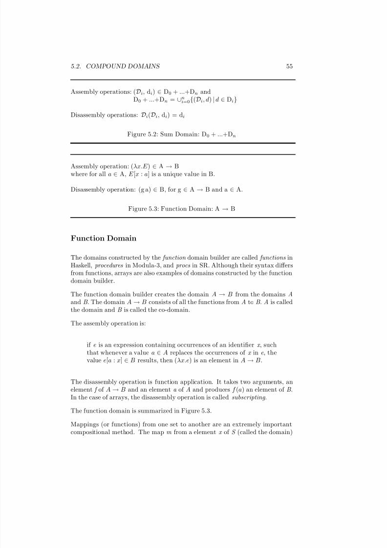
7/3/2019 Theory Introduction to Programming Languages
http://slidepdf.com/reader/full/theory-introduction-to-programming-languages-5584618bb4249 69/233
5.2. COMPOUND DOMAINS 55
Assembly operations: (Di, di) ∈ D0 + ...+Dn andD0 + ...+Dn = ∪n
i=0{(Di, d) | d ∈ Di}
Disassembly operations: Di(Di, di) = di
Figure 5.2: Sum Domain: D0 + ...+Dn
Assembly operation: (λx.E ) ∈ A → Bwhere for all a ∈ A, E [x : a] is a unique value in B.
Disassembly operation: (g a) ∈ B, for g ∈ A → B and a ∈ A.
Figure 5.3: Function Domain: A → B
Function Domain
The domains constructed by the function domain builder are called functions inHaskell, procedures in Modula-3, and procs in SR. Although their syntax differsfrom functions, arrays are also examples of domains constructed by the functiondomain builder.
The function domain builder creates the domain A → B from the domains Aand B . The domain A → B consists of all the functions from A to B . A is calledthe domain and B is called the co-domain.
The assembly operation is:
if e is an expression containing occurrences of an identifier x , suchthat whenever a value a ∈ A replaces the occurrences of x in e, thevalue e[a : x] ∈ B results, then (λx.e) is an element in A → B.
The disassembly operation is function application. It takes two arguments, anelement f of A → B and an element a of A and produces f (a) an element of B .In the case of arrays, the disassembly operation is called subscripting .
The function domain is summarized in Figure 5.3.
Mappings (or functions) from one set to another are an extremely importantcompositional method. The map m from a element x of S (called the domain)
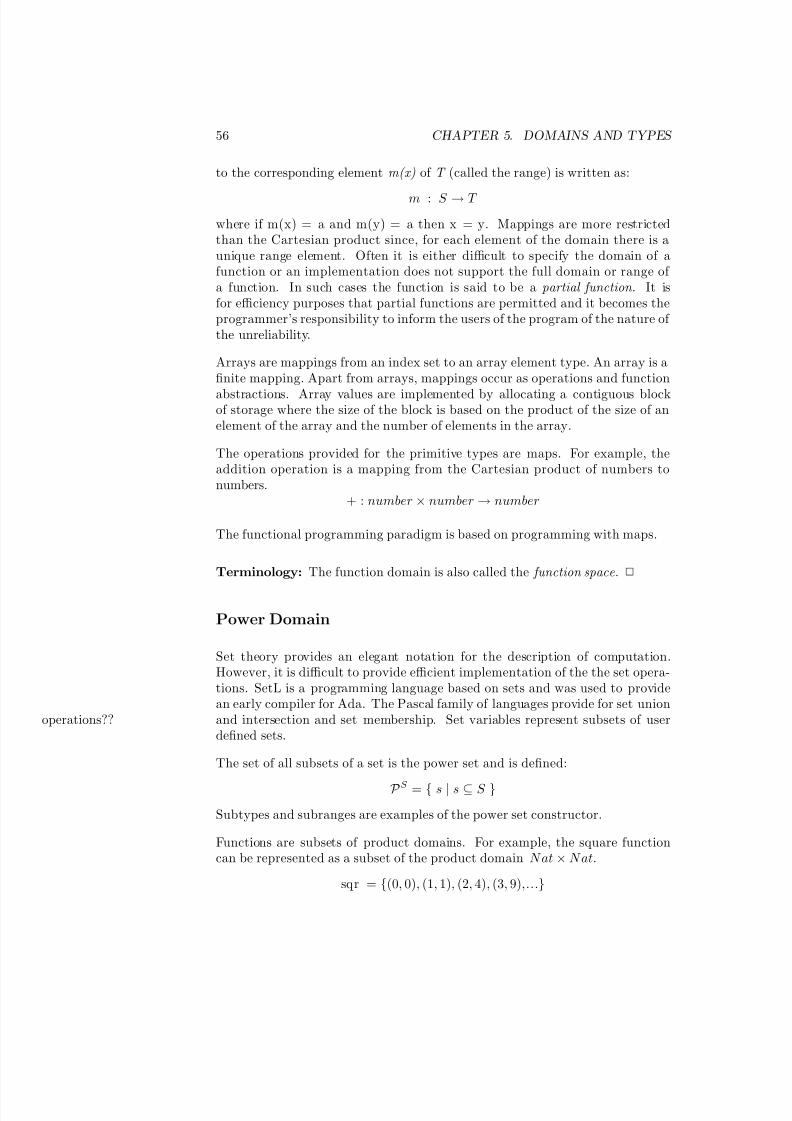
7/3/2019 Theory Introduction to Programming Languages
http://slidepdf.com/reader/full/theory-introduction-to-programming-languages-5584618bb4249 70/233
56 CHAPTER 5. DOMAINS AND TYPES
to the corresponding element m(x) of T (called the range) is written as:
m : S → T
where if m(x) = a and m(y) = a then x = y. Mappings are more restrictedthan the Cartesian product since, for each element of the domain there is aunique range element. Often it is either difficult to specify the domain of afunction or an implementation does not support the full domain or range of a function. In such cases the function is said to be a partial function . It isfor efficiency purposes that partial functions are permitted and it becomes theprogrammer’s responsibility to inform the users of the program of the nature of the unreliability.
Arrays are mappings from an index set to an array element type. An array is afinite mapping. Apart from arrays, mappings occur as operations and function
abstractions. Array values are implemented by allocating a contiguous blockof storage where the size of the block is based on the product of the size of anelement of the array and the number of elements in the array.
The operations provided for the primitive types are maps. For example, theaddition operation is a mapping from the Cartesian product of numbers tonumbers.
+ : number × number → number
The functional programming paradigm is based on programming with maps.
Terminology: The function domain is also called the function space. 2
Power Domain
Set theory provides an elegant notation for the description of computation.However, it is difficult to provide efficient implementation of the the set opera-tions. SetL is a programming language based on sets and was used to providean early compiler for Ada. The Pascal family of languages provide for set unionand intersection and set membership. Set variables represent subsets of useroperations??defined sets.
The set of all subsets of a set is the power set and is defined:
P S = { s | s ⊆ S }
Subtypes and subranges are examples of the power set constructor.
Functions are subsets of product domains. For example, the square functioncan be represented as a subset of the product domain N at × N at.
sqr = {(0, 0), (1, 1), (2, 4), (3, 9),...}
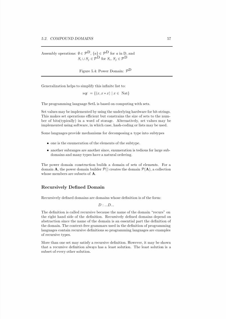
7/3/2019 Theory Introduction to Programming Languages
http://slidepdf.com/reader/full/theory-introduction-to-programming-languages-5584618bb4249 71/233
5.2. COMPOUND DOMAINS 57
Assembly operations: ∅ ∈ P D, {a} ∈ P D for a in D, and
S i ∪ S j ∈ P D for S i, S j ∈ P D
Figure 5.4: Power Domain: P D
Generalization helps to simplify this infinite list to:
sqr = {(x, x ∗ x) | x ∈ Nat}
The programming language SetL is based on computing with sets.
Set values may be implemented by using the underlying hardware for bit-strings.This makes set operations efficient but constrains the size of sets to the num-ber of bits(typically) in a word of storage. Alternatively, set values may beimplemented using software, in which case, hash-coding or lists may be used.
Some languages provide mechanisms for decomposing a type into subtypes
• one is the enumeration of the elements of the subtype.
• another subranges are another since, enumeration is tedious for large sub-domains and many types have a natural ordering.
The power domain construction builds a domain of sets of elements. For adomain A, the power domain builder P () creates the domain P (A), a collectionwhose members are subsets of A.
Recursively Defined Domain
Recursively defined domains are domains whose definition is of the form:
D : ...D...
The definition is called recursive because the name of the domain “recurs” onthe right hand side of the definition. Recursively defined domains depend onabstraction since the name of the domain is an essential part the definition of the domain. The context-free grammars used in the definition of programminglanguages contain recursive definitions so programming languages are examplesof recursive types.
More than one set may satisfy a recursive definition. However, it may be shownthat a recursive definition always has a least solution. The least solution is asubset of every other solution.
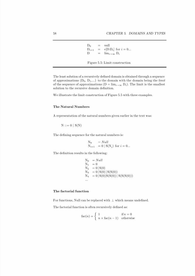
7/3/2019 Theory Introduction to Programming Languages
http://slidepdf.com/reader/full/theory-introduction-to-programming-languages-5584618bb4249 72/233
58 CHAPTER 5. DOMAINS AND TYPES
D0 = null
Di+1 = e[D:Di] for i = 0...D = limi→∞ Di
Figure 5.5: Limit construction
The least solution of a recursively defined domain is obtained through a sequenceof approximations (D0, D1,...) to the domain with the domain being the limit of the sequence of approximations (D = limi→∞ Di). The limit is the smallestsolution to the recursive domain definition.
We illustrate the limit construction of Figure 5.5 with three examples.
The Natural Numbers
A representation of the natural numbers given earlier in the text was:
N ::= 0 | S(N)
The defining sequence for the natural numbers is:
N0 = Null
Ni+1 = 0 | S(Ni) for i = 0...
The definition results in the following:
N0 = NullN1 = 0N2 = 0 | S(0)N3 = 0 | S(0) | S(S(0))N4 = 0 | S(0)|S(S(0)) | S(S(S(0)))...
The factorial function
For functions, Null can be replaced with ⊥ which means undefined.
The factorial function is often recursively defined as:
fac(n) =
1 if n = 0n × fac(n − 1) otherwise
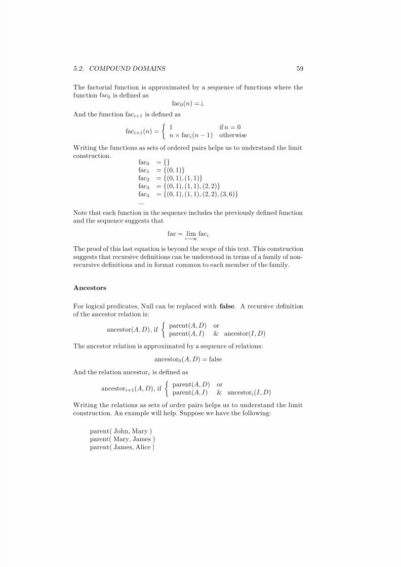
7/3/2019 Theory Introduction to Programming Languages
http://slidepdf.com/reader/full/theory-introduction-to-programming-languages-5584618bb4249 73/233
5.2. COMPOUND DOMAINS 59
The factorial function is approximated by a sequence of functions where thefunction fac0 is defined as
fac0(n) =⊥
And the function faci+1 is defined as
faci+1(n) =
1 if n = 0n × faci(n − 1) otherwise
Writing the functions as sets of ordered pairs helps us to understand the limitconstruction.
fac0 = {}fac1 = {(0, 1)}fac2 = {(0, 1), (1, 1)}fac3 = {(0, 1), (1, 1), (2, 2)}fac4 = {(0, 1), (1, 1), (2, 2), (3, 6)}...
Note that each function in the sequence includes the previously defined functionand the sequence suggests that
fac = limi→∞
faci
The proof of this last equation is beyond the scope of this text. This constructionsuggests that recursive definitions can be understood in terms of a family of non-recursive definitions and in format common to each member of the family.
Ancestors
For logical predicates, Null can be replaced with false. A recursive definitionof the ancestor relation is:
ancestor(A, D), if
parent(A, D) orparent(A, I ) & ancestor(I, D)
The ancestor relation is approximated by a sequence of relations:
ancestor0(A, D) = false
And the relation ancestori is defined as
ancestori+1(A, D), if
parent(A, D) orparent(A, I ) & ancestori(I, D)
Writing the relations as sets of order pairs helps us to understand the limitconstruction. An example will help. Suppose we have the following:
parent( John, Mary )parent( Mary, James )parent( James, Alice )
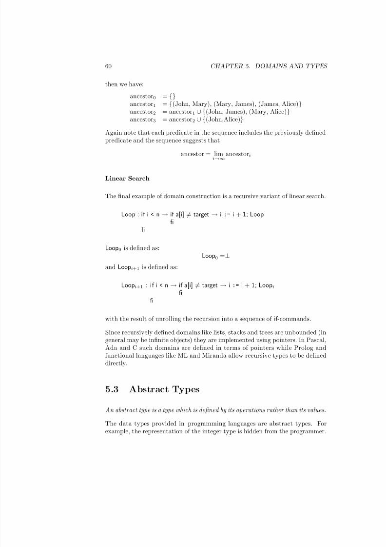
7/3/2019 Theory Introduction to Programming Languages
http://slidepdf.com/reader/full/theory-introduction-to-programming-languages-5584618bb4249 74/233
60 CHAPTER 5. DOMAINS AND TYPES
then we have:
ancestor0 = {}ancestor1 = {(John, Mary), (Mary, James), (James, Alice)}ancestor2 = ancestor1 ∪ {(John, James), (Mary, Alice)}ancestor3 = ancestor2 ∪ {(John,Alice)}
Again note that each predicate in the sequence includes the previously definedpredicate and the sequence suggests that
ancestor = limi→∞
ancestori
Linear Search
The final example of domain construction is a recursive variant of linear search.
Loop : if i < n → if a[i] = target → i := i + 1; Loopfi
fi
Loop0 is defined as:Loop0 =⊥
and Loopi+1 is defined as:
Loopi+1 : if i < n → if a[i] = target → i := i + 1; Loopififi
with the result of unrolling the recursion into a sequence of if -commands.
Since recursively defined domains like lists, stacks and trees are unbounded (ingeneral may be infinite objects) they are implemented using pointers. In Pascal,Ada and C such domains are defined in terms of pointers while Prolog andfunctional languages like ML and Miranda allow recursive types to be defineddirectly.
5.3 Abstract Types
An abstract type is a type which is defined by its operations rather than its values.
The data types provided in programming languages are abstract types. Forexample, the representation of the integer type is hidden from the programmer.
7/3/2019 Theory Introduction to Programming Languages
http://slidepdf.com/reader/full/theory-introduction-to-programming-languages-5584618bb4249 75/233
5.3. ABSTRACT TYPES 61
The programmer is provided with a set of operations and a high-level represen-tation of integers. The programmer only becomes aware of the lower level whenan arithmetic overflow occurs.
An Abstract data type consists of a type name and operations for creating andmanipulating objects of the type. A key idea is that of the separation of theimplementation from the type definition. The actual format of the data is hidden(information hiding) from the user and the user gains access to the data onlythrough the type operations.
There are two advantages to defining an abstract type as a set of operations.First, the separation of operations from the representation results in data in-dependence. Second, the operations can be defined in a rigorous mathematicalmanner. As indicated in Chapter 3, algebraic definitions provide appropriate
method for defining an abstract type. The formal specification of an abstracttype can be separated into two parts. A syntactic specification with gives thesignature of the operations and a semantic part in which axioms describe theproperties of the operations.
In order to be fully abstract, the user of the abstract type must not be per-mitted access to the representation of values of the type. This is the case withthe primitive types. For example, integers might be represented in two’s com-plement binary numbers but there is no way of finding out the representationwithout going outside the language. Thus, a key concept of abstract types isthe hiding of the representation of the values of the type. This means that therepresentation information must be local to the type definition.
Modula-3’s approach is typical. An abstract type is defined using Modules – adefinition module (called an interface), and an implementation module (calleda module).
Since the representation of the values of the type is hidden, abstract typesmust be provided with constructor and destructor operations. A constructoroperation composes a value of the type from values from some other type or typeswhile a destructor operation extracts a constituent value from an abstract type.For example, an abstract type for rational numbers might represent rationalnumbers as pairs of integers. This means that the definition of the abstracttype would include an operation which given a pair of integers returns a rationalnumber (whose representation as an ordered pair is hidden) which correspondsto the the quotient of the two numbers. The rational additive and multiplicative
identities corresponding to zero and one would be provided also.
Figure 5.6 is a definition definition module of an abstract type for complexnumbers using Modula-2 and 5.7 is the corresponding implementation module.
Terminology: The terms abstract data type and ADT are also used to denotewhat we call an abstract type. 2

7/3/2019 Theory Introduction to Programming Languages
http://slidepdf.com/reader/full/theory-introduction-to-programming-languages-5584618bb4249 76/233
62 CHAPTER 5. DOMAINS AND TYPES
DEFINITION MODULEComplexNumbers;
TYPE Complex;
PROCEDURE MakeComplex ( firstNum, secondNum : Real ) : Complex;
PROCEDURE AddComplex ( firstNum, secondNum : Complex ) : Complex;
PROCEDURE MultiplyComplex ( firstNum, secondNum : Complex ) : Complex;...END ComplexNumbers.
Figure 5.6: Complex numbers abstract type
IMPLEMENTATION MODULE ComplexNumbers;
TYPE
Complex = POINTER TO ComplexDataComplexData = RECORD
RealPart, ImPart : REAL;END;
PROCEDURE MakeComplex ( firstNum, secondNum : Real ) : Complex;VAR result : Complex;
BEGIN
new( result );
result↑.RealPart := firstNum;result↑.ImPart := secondNumreturn result
END NewComplex;
PROCEDURE AddComplex ( firstNum, secondNum : Complex ) : Complex;VAR result : Complex;
BEGIN
new( result );result↑.RealPart := firstNum↑.RealPart + secondNum↑.RealPart;result↑.ImPart := firstNum↑.ImPart + secondNum↑.ImPartreturn result
END AddComplex;
...
BEGIN
...END ComplexNumbers.
Figure 5.7: Complex numbers implementation
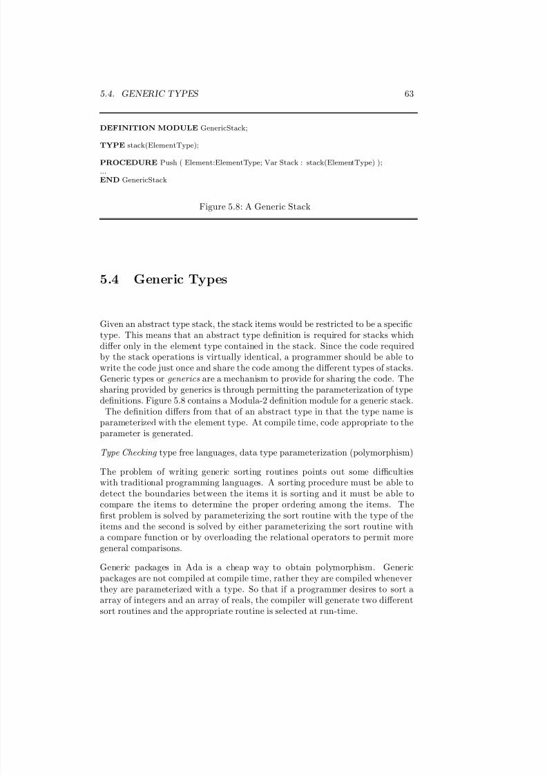
7/3/2019 Theory Introduction to Programming Languages
http://slidepdf.com/reader/full/theory-introduction-to-programming-languages-5584618bb4249 77/233
5.4. GENERIC TYPES 63
DEFINITION MODULE GenericStack;
TYPE stack(ElementType);
PROCEDURE Push ( Element:ElementType; Var Stack : stack(ElementType) );...END GenericStack
Figure 5.8: A Generic Stack
5.4 Generic Types
Given an abstract type stack, the stack items would be restricted to be a specifictype. This means that an abstract type definition is required for stacks whichdiffer only in the element type contained in the stack. Since the code requiredby the stack operations is virtually identical, a programmer should be able towrite the code just once and share the code among the different types of stacks.Generic types or generics are a mechanism to provide for sharing the code. Thesharing provided by generics is through permitting the parameterization of typedefinitions. Figure 5.8 contains a Modula-2 definition module for a generic stack.
The definition differs from that of an abstract type in that the type name isparameterized with the element type. At compile time, code appropriate to theparameter is generated.
Type Checking type free languages, data type parameterization (polymorphism)
The problem of writing generic sorting routines points out some difficultieswith traditional programming languages. A sorting procedure must be able todetect the boundaries between the items it is sorting and it must be able tocompare the items to determine the proper ordering among the items. Thefirst problem is solved by parameterizing the sort routine with the type of theitems and the second is solved by either parameterizing the sort routine witha compare function or by overloading the relational operators to permit moregeneral comparisons.
Generic packages in Ada is a cheap way to obtain polymorphism. Genericpackages are not compiled at compile time, rather they are compiled wheneverthey are parameterized with a type. So that if a programmer desires to sort aarray of integers and an array of reals, the compiler will generate two differentsort routines and the appropriate routine is selected at run-time.
7/3/2019 Theory Introduction to Programming Languages
http://slidepdf.com/reader/full/theory-introduction-to-programming-languages-5584618bb4249 78/233
64 CHAPTER 5. DOMAINS AND TYPES
5.5 Type Systems
Definition 5.1 A type system is a set of rules for associating a type with ex-pression in the language. A type system rejects an expression if it does not associate a type with the expression.
A type system is monomorphic if each constant, variable, parameter, and func-tion result has a unique type. Type checking in a monomorphic system isstraightforward. But purely monomorphic type systems are unsatisfactory forwriting reuseable software. Many algorithms such as sorting and list and treemanipulation routines are generic in the sense that they depend very little on
the type of the values being manipulated. For example, a general purpose arraysorting routine cannot be written in Pascal. Pascal requires that the elementtype of the array be part of the declaration of the routine. This means thatdifferent sorting routines must be written for each element type and array size.
A large percentage of errors in programs is due to the application of operationsto objects of incompatible types. To assist the programmer in the detectionof these errors, several schemes have been developed. If the errors are to bedetected at compile time then a static type checking system is required. Oneapproach to static type checking is to require the programmer to specify thetype of each object in the program. This permits the compiler to perform typechecking before the execution of the program and this is the approach taken bylanguages like Pascal and Ada. Another approach to static type checking is toadd type inference capabilities to the compiler. In such a system the compilerperforms type checking by means of a set of type inference rules and is able toflag type errors prior to runtime. This is the approach taken by Miranda andHaskell but they also permit programmer to provide type specifications.
If the error detection is to be delayed until execution time, then dynamic typechecking is required. The programming languages Scheme and Prolog do notrequire the programmer to provide any information concerning an object’s typeand type checking is necessarily delayed until run time.
Neither Prolog, Scheme or Miranda require type declarations. Types may bedeclared in Miranda. For example the types for the arithmetic + operation aredeclared as follows:
+ :: num -> num -> num
Modula-2, Ada, C++, Prolog, Scheme, Miranda – list primitive types
7/3/2019 Theory Introduction to Programming Languages
http://slidepdf.com/reader/full/theory-introduction-to-programming-languages-5584618bb4249 79/233
5.5. TYPE SYSTEMS 65
Type Equivalence
Two unnamed types (sets of objects) are the same if they contain the sameelements. The same cannot be said of named types for if they were, then therewould be no need for the disjoint union type. When types are named, there aretwo major approaches to determining whether two types are equal.
Name Equivalence
In name equivalence two types are the same iff they have the same name. Nameequivalence was chosen for Modula-2, Ada, C (for records), and Miranda andrequires type definitions to be global. The predecessor of Modula-2, Pascalviolates name equivalence since file type names are not required to be sharedby different programs accessing the same file.
Structural Equivalence
In structural equivalence, the names of the types are ignored and the elementsof the types are compared for equality. Formally,
Definition 5.2 Two types T, T are structurally equivalent iff T, T have thesame set of values.
The following three rules may be used to determine if two types are structurallyequivalent.
• A type name is structurally equivalent to its self.
• Two types are structurally equivalent if they are formed by applying thesame type constructor to structurally equivalent types.
• After a type declaration , type n = T , the type name n is structurallyequivalent to T .
Structural equivalence was chosen by Algol-68 and C (except for records) be-cause it is easy to implement and type definitions are not required to be global.
Strong vs. Weak Type Checking
Definition 5.3 A language is said to be strongly typed if it enforces type ab-stractions. That is, operations may be applied only to objects of the appropriatetype.
7/3/2019 Theory Introduction to Programming Languages
http://slidepdf.com/reader/full/theory-introduction-to-programming-languages-5584618bb4249 80/233
66 CHAPTER 5. DOMAINS AND TYPES
The language is said to be weakly typed.
For example, if the boolean constants are represented by 0 and 1 and the lan-guage permits a boolean to occur in arithmetic expressions, then the languageis not enforcing the boolean type abstraction.
Most languages are strongly typed with respect to the primitive types supportedby the language.
Strong typing helps to insure the security and portability of the code and itoften requires the programmer to explicitly define the types of each object in aprogram.
SORT PROGRAMS
Weak type checking has the advantage of providing representation indepen-dence.
SETS VS LISTS
Type Inference
Pascal constant declarations are an example of type inference, the type of thename is inferred from the type of the constant. In Pascal’s for loop the type of the loop index can be inferred from the types of the loop limits and thus theloop index should be a variable local to the loop. The programming languageMiranda provides a powerful type inference system so that a programmer neednot declare any types. However, Miranda is strongly typed.
A type checker must be able to
• determine if a program is well typed and
• if the program is well typed, determine the type of any expression in theprogram.
Type inference axioms
Axiom 5.1 given that: f is of type A → B and x is of type A
infer that: f(x) is type correct and has type B
Static vs Dynamic type checking
If a language requires that the type of all variables be known compile time,then the a language is said to be statically typed . Pascal, Ada, and Haskell are
7/3/2019 Theory Introduction to Programming Languages
http://slidepdf.com/reader/full/theory-introduction-to-programming-languages-5584618bb4249 81/233
5.6. OVERLOADING AND POLYMORPHISM 67
examples of statically typed languages.
Static typing is widely recognized as a requirement for the production of safeand reliable software.
If a language does not require that the type of a variable be known at compiletime, then a language is said to be dynamically typed . Lisp and Smalltalk areexamples of dynamically typed languages.
Dynamic type checking implies that the types are checked at execution timeand that every value is tagged to identify its type in order to make the typechecking possible. The penalty for dynamic type checking is additional spaceand time overheads.
Dynamic typing is often justified on the assumption that its flexibility permits
the rapid prototyping of software.
Prolog relies on pattern matching to provide a semblance of type checking.There is active research on adapting type checking systems for Prolog.
Modern functional programming languages such as Miranda and Haskell com-bine the safety of static type checking with the flexibility of dynamic type check-ing through polymorphic types.
5.6 Overloading and Polymorphism
Overloading
Completely monomorphic systems are rare. Most programming languages con-tain some operators or procedures which permit arguments of more than onetype. For example, Pascal’s input and output procedures permit variation bothin type and in number of arguments. This is an example of overloading .
Definition 5.4 Overloading refers to the use of a single syntactic identifier torefer to several different operations discriminated by the type and number of thearguments to the operation.
The type of the plus operation defined for integer addition is
+ : int × int → int
When the same operation symbol is used for the plus operation for rationalnumbers and for set union, the symbol as in Pascal it is overloaded. Mostprogramming languages provide for the overloading of the arithmetic operators.
7/3/2019 Theory Introduction to Programming Languages
http://slidepdf.com/reader/full/theory-introduction-to-programming-languages-5584618bb4249 82/233
68 CHAPTER 5. DOMAINS AND TYPES
A few programming languages (Ada among others) provide for programmerdefined overloading of both built-in and programmer defined operators.
When overloaded operators are applied to mixed expressions such as plus toan integer and a rational number there are two possible choices. Either theevaluation of the expression fails or one or more of the subexpressions are coerced into a corresponding object of another type. Integers are often coerced intothe corresponding rational number. This type of coercion is called widening .When a language permits the coercion of a real number into an integer (bytruncation for example) the coercion is called narrowing . Narrowing is notusually permitted in a programming language since information is usually lost.Coercion is an issue in programming languages because numbers do not havea uniform representation. This type of overloading is called context-dependent overloading .
Many languages provide type transfer functions so that the programmer cancontrol where and when the type coercion is performed. Truncate and roundare examples of type transfer functions.
Overloading is sometimes called ad-hoc polymorphism .
Polymorphism
A type system is polymorphic if abstractions operate uniformly on arguments of a family of related types.
Definition 5.5 A polymorphic operation is one that can be applied to different but related types of arguments.
This type of polymorphism is sometimes called parametric polymorphism .
Generalization can be applied to may aspects of programming languages.
Sometimes there are several domains which share a common operation. Forexample, the natural numbers, the integers, the rationals, and the reals allshare the operation of addition. So, most programming languages use the sameaddition operator to denote addition in all of these domains. Pascal extends theuse of the addition operator to represent set union. The multiple use of a namein different domains is called overloading . Ada permits user defined overloadingof built in operators.
Prolog permits the programmer to use the same functor name for predicatesof different arity thus permitting the overloading of functor names. This is anexample of data generalization or polymorphism.
7/3/2019 Theory Introduction to Programming Languages
http://slidepdf.com/reader/full/theory-introduction-to-programming-languages-5584618bb4249 83/233
5.7. TYPE COMPLETENESS 69
While the parameterization of an object gives the ability to deal with more thanone particular object, polymorphism is the ability of an operation to deal withobjects of more than a single type.
Generalization of control has focused on advanced control structures (RAM):iterators, generators, backtracking, exception handling, coroutines, and parallelexecution (processes).
5.7 Type Completeness
5.8 Exercises
1. Define algebraic semantics for the following data types.
(a) Boolean
ADTBoolean
Operations
and(boolean,boolean) → boolean
or(boolean,boolean) → boolean
not(boolean) → boolean
Semantic Equationsand(true,true) = true
or(true,true) = true
not(true) = false
not(false) = true
Restrictions
(b) Integer
(c) Real
(d) Character
(e) String2. Name or Structure equivalence (type checking)
3. Algebraic Semantics: stack, tree, queue, grade book etc
4. Abstraction
5. Generalization

7/3/2019 Theory Introduction to Programming Languages
http://slidepdf.com/reader/full/theory-introduction-to-programming-languages-5584618bb4249 84/233
70 CHAPTER 5. DOMAINS AND TYPES
6. Name or Structure equivalence (type checking)
7. Extend the compiler to handle additional types. This requires modifica-tions to the syntax of the language with extensions of the scanner, parser,symbol table and code generators.
7/3/2019 Theory Introduction to Programming Languages
http://slidepdf.com/reader/full/theory-introduction-to-programming-languages-5584618bb4249 85/233
Chapter 6
Environment
Keywords and phrases: block, garbage collection, static and dynamic links,display, static and dynamic binding, activation record, environment, Static andDynamic Scope, aliasing, variables, value, result, value-result, reference, name,unification, eager evaluation, lazy evaluation, strict, non-strict, Church-Rosser,overloading, polymorphism, monomorphism, coercion, transfer functions.
An environment is a set of bindings.
Scope has to do with the range of visibility of names. For example, a na-tional boundary may encapsulate a natural language. However, some wordsused within the boundary are not native words. They are words borrowed fromsome other language and are defined in that foreign language. So it is in aprogram. A definition introduces a name and a boundary ( the object ). Theobject may contain names for which there is no local definition (assuming defi-nitions may be nested). These names are said to be free. The meaning assignedto these names is to be found outside of the definition. The rules followed in
determining the meaning of these free names are called scope rules.
Scope is the portion of the program text over which a definition is effective.
It is concerned with name control.
71
7/3/2019 Theory Introduction to Programming Languages
http://slidepdf.com/reader/full/theory-introduction-to-programming-languages-5584618bb4249 86/233
72 CHAPTER 6. ENVIRONMENT
Binding Sequence
Typically the text of a program contains a number of bindings between namesand objects and the bindings may be composed collaterally, sequentially orrecursively.
Collateral
A collateral binding is to perform the bindings independently of each other andthen to combine the bindings to produce the completed set of bindings. Netherbinding can reference a name used in any other binding.
Collateral bindings are not vary common but occur in Scheme and ML.
Sequential
The most common way of composing bindings is sequentially. A sequential binding is to perform the bindings in the sequence in which they occur. Theeffect is to allow later bindings to use bindings produced earlier in the sequence.It must be noted that sequential bindings do not permit mutually recursivedefinitions.
In Pascal, constant, variable, and procedure and function bindings are sequen-tial. To provide for mutually recursive definitions of functions and procedures,
Pascal provides for the separation of the signature of a function or procedurefrom the body by the means of forward declarations so that so that mutuallyrecursive definitions may be constructed.
Recursive
A recursive binding is one that uses the very bindings that it produces itself.In Pascal type definitions are recursive to permit the construction of recursivetypes. However, there is a constraint to insure that recursive types are restrictedto pointer types.
6.1 Block structure
A block is a construct that delimits the scope of any declarations that it maycontain. It provides a local environment i.e., a opportunity for local definitions.The block structure (the textual relationship between blocks) of a programming

7/3/2019 Theory Introduction to Programming Languages
http://slidepdf.com/reader/full/theory-introduction-to-programming-languages-5584618bb4249 87/233
6.1. BLOCK STRUCTURE 73
language has a great deal of influence over program structure and modularity.There are three basic block structures–monolithic, flat and nested.
A program has a monolithic block structure if it consists of just one block. Thisstructure is typical of BASIC and early versions of COBOL. The monolithicstructure is suitable only for small programs. The scope of every definition isthe entire program. Typically all definitions are grouped in one place even if they are used in different parts of the program.
A program has a flat block structure if it is partitioned into distinct blocks, anouter all inclosing block one or more inner blocks. This structure is typical of FORTRAN and C. In these languages, all subprograms (procedures and func-tions) are separate, and each acts as a block. Variables can be declared insidea subprogram are then local to that subprogram. Subprogram names are part
of the outer block and thus their scope is the entire program along with globalvariables. All subprogram names and global variables must be unique. If avariable cannot be local to a subprogram then it must be global and accessableby all subprograms even though it is used in only a couple of subprograms.
A program has nested block structure if blocks may be nested inside other blocks.This is typical of the block structure of the Algol-like languages. A block canbe located close to the point of use.
A local variable is one that is declared within a block for use only within thatblock.
A global variable is a variable that is referenced within a block but declaredoutside the block.
An activation of a block is a time interval during which that block is beingexecuted.
The three basic block structures are sufficient for what is called programming in the small . These are programs which are comprehensible in their entirety by anindividual programmer. They are not general enough for very large programs.Programs which are written by many individual and which must consist of module which can be developed and tested independently of other modules.Such programming is called programming in the large. The subject of moduleswill be examined in a later chapter.
Activation Records
Each block
Storage for local variables.
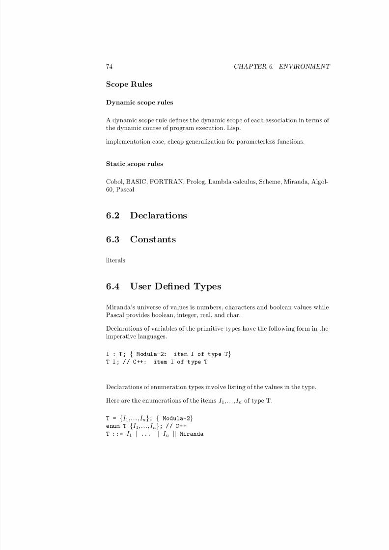
7/3/2019 Theory Introduction to Programming Languages
http://slidepdf.com/reader/full/theory-introduction-to-programming-languages-5584618bb4249 88/233
74 CHAPTER 6. ENVIRONMENT
Scope Rules
Dynamic scope rules
A dynamic scope rule defines the dynamic scope of each association in terms of the dynamic course of program execution. Lisp.
implementation ease, cheap generalization for parameterless functions.
Static scope rules
Cobol, BASIC, FORTRAN, Prolog, Lambda calculus, Scheme, Miranda, Algol-
60, Pascal
6.2 Declarations
6.3 Constants
literals
6.4 User Defined Types
Miranda’s universe of values is numbers, characters and boolean values whilePascal provides boolean, integer, real, and char.
Declarations of variables of the primitive types have the following form in theimperative languages.
I : T ; { Modula-2: item I of type T}T I; // C++: item I of type T
Declarations of enumeration types involve listing of the values in the type.
Here are the enumerations of the items I 1,...,I n of type T.
T = {I 1,...,I n}; { Modula-2}enum T {I 1,...,I n}; // C++
T ::= I 1 | ... | I n || Miranda
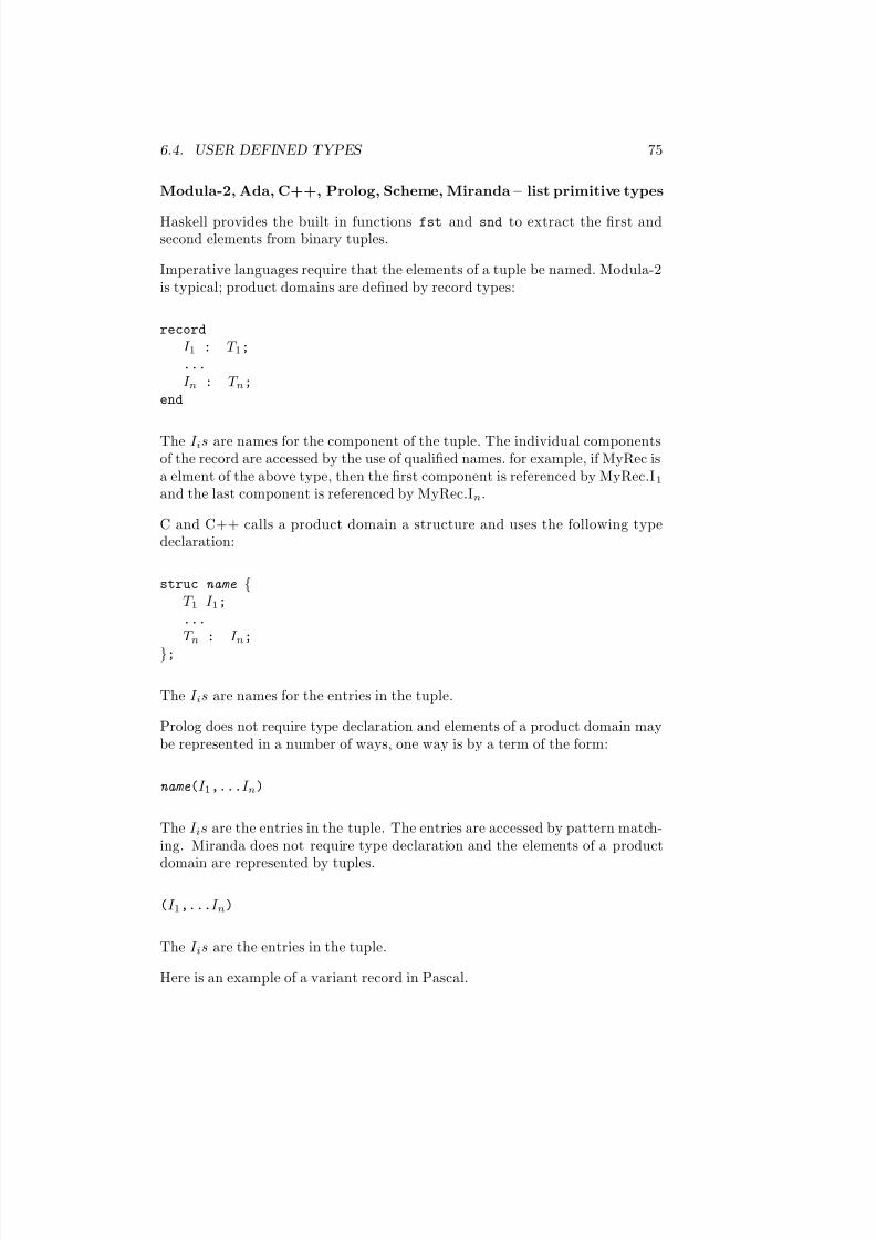
7/3/2019 Theory Introduction to Programming Languages
http://slidepdf.com/reader/full/theory-introduction-to-programming-languages-5584618bb4249 89/233
6.4. USER DEFINED TYPES 75
Modula-2, Ada, C++, Prolog, Scheme, Miranda – list primitive types
Haskell provides the built in functions fst and snd to extract the first andsecond elements from binary tuples.
Imperative languages require that the elements of a tuple be named. Modula-2is typical; product domains are defined by record types:
record
I 1 : T 1;
...
I n : T n;
end
The I is are names for the component of the tuple. The individual componentsof the record are accessed by the use of qualified names. for example, if MyRec isa elment of the above type, then the first component is referenced by MyRec.I1and the last component is referenced by MyRec.In.
C and C++ calls a product domain a structure and uses the following typedeclaration:
struc name {T 1 I 1;
...
T n : I n;
};
The I is are names for the entries in the tuple.
Prolog does not require type declaration and elements of a product domain maybe represented in a number of ways, one way is by a term of the form:
name(I 1,...I n)
The I is are the entries in the tuple. The entries are accessed by pattern match-ing. Miranda does not require type declaration and the elements of a product
domain are represented by tuples.
(I 1,...I n)
The I is are the entries in the tuple.
Here is an example of a variant record in Pascal.
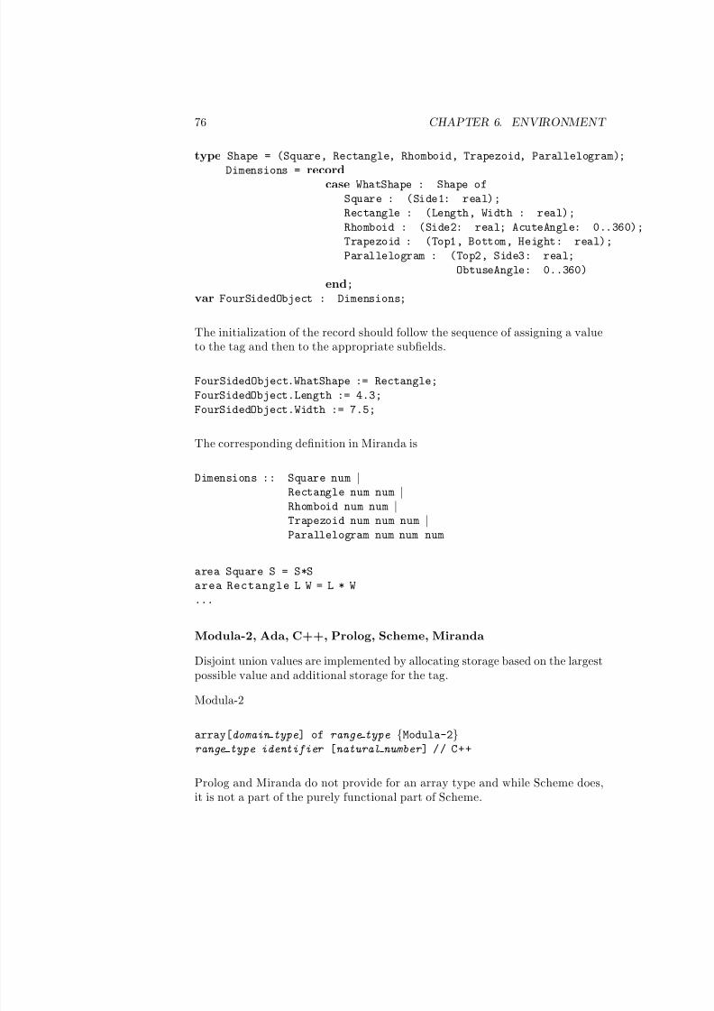
7/3/2019 Theory Introduction to Programming Languages
http://slidepdf.com/reader/full/theory-introduction-to-programming-languages-5584618bb4249 90/233
76 CHAPTER 6. ENVIRONMENT
type Shape = (Square, Rectangle, Rhomboid, Trapezoid, Parallelogram);
Dimensions = recordcase WhatShape : Shape of
Square : (Side1: real);
Rectangle : (Length, Width : real);
Rhomboid : (Side2: real; AcuteAngle: 0..360);
Trapezoid : (Top1, Bottom, Height: real);
Parallelogram : (Top2, Side3: real;
ObtuseAngle: 0..360)
end;
var FourSidedObject : Dimensions;
The initialization of the record should follow the sequence of assigning a valueto the tag and then to the appropriate subfields.
FourSidedObject.WhatShape := Rectangle;
FourSidedObject.Length := 4.3;
FourSidedObject.Width := 7.5;
The corresponding definition in Miranda is
Dimensions :: Square num |Rectangle num num |Rhomboid num num |Trapezoid num num num |
Parallelogram num num num
area Square S = S*S
area Rectangle L W = L * W
...
Modula-2, Ada, C++, Prolog, Scheme, Miranda
Disjoint union values are implemented by allocating storage based on the largestpossible value and additional storage for the tag.
Modula-2
array[domain type] of range type {Modula-2}range type identifier [natural number ] // C++
Prolog and Miranda do not provide for an array type and while Scheme does,it is not a part of the purely functional part of Scheme.

7/3/2019 Theory Introduction to Programming Languages
http://slidepdf.com/reader/full/theory-introduction-to-programming-languages-5584618bb4249 91/233
6.4. USER DEFINED TYPES 77
Modula-2, Ada, C++, Prolog, Scheme, Miranda – mapping type
In Pascal the notation [i..j] indicates the subset of an ordinal type from elementi to element j inclusive. In addition to subranges, Miranda provides infinitelists [i..] and finite and infinite arithmetic series [a,b..c], [a,b..] (the interval is(b-a)). Miranda also provides list comprehensions which are used to constructlists (sets). A list comprehension has the form [exp | qualifier]
sqs = [ n*n | n < −[1..] ]
factors n = [ r | r < −[1..n div 2]; n mod r = 0 ]
knights moves [i,j] = [ [i+a,j+b] | a,b < −[−2..2]; a^2+^2=5 ]
Modula-2, Ada, C++, Prolog, Scheme, Miranda – power set
Prolog
[ ]
The Miranda syntax for lists is similar to that of Prolog however, elements of lists must be all of the same type.
[*]
Recursive types in imperative programming languages are usually defined usinga pointer type. Pointer types are an additional primitive type. Pointers areaddresses.
{Modula-2: the pointer and the list}type NextItem = ^ListType
ListType = recorditem : Itemtype;
next : NextItem
end;
// C++: the list type
struc list {ItemType Item;
list* Next; // pointer to list
};
|| Miranda: list of objects of type T and
|| a binary tree of type T

7/3/2019 Theory Introduction to Programming Languages
http://slidepdf.com/reader/full/theory-introduction-to-programming-languages-5584618bb4249 92/233
78 CHAPTER 6. ENVIRONMENT
[ T ]
tree ::= Niltree | Node T tree tree
Referencing/Dereferencing
type ListType = recorditem : Itemtype;
next : ListType
end;
Recursive values are implemented using pointers. The run-time support systemfor the functional and logic programming languages, provides for automaticallocation and recovery of storage (garbage collection). The alternative is forthe language to provide access to the run-time system so that the programmercan explicitly allocate and recover the linked structures.
6.5 Variablesstate:store
It is frequently necessary to refer to an arbitrary element of a type. Such areference is provided through the use of variables. A variable is a name for anarbitrary element of a type and it is a generalization of a value since it can bethe name of any element.
6.6 Functions and Procedures
6.7 Persistant Types
A persistent variable is one whose lifetime transcends an activation of any partic-ular program. In contrast, a transient variable is one whose lifetime is boundedby the activation of the program that created it. Local and heap variables aretransient variables.
Most programming languages provide different types for persistent and transientvariables. Typically files are the only type of persistent variable permitted in aprogramming language. Files are not usually permitted to be transient variables.
Most programming languages provide different types for persistent and transientThe type completeness principle suggests that all the types of the programminglanguage should be allowed both for transient variables and persistent variables.A language applying this principle would be simplified by having no special

7/3/2019 Theory Introduction to Programming Languages
http://slidepdf.com/reader/full/theory-introduction-to-programming-languages-5584618bb4249 93/233
6.8. EXERCISES 79
types, commands or procedures for input–output. The programmer would bespared the effort of converting data from a persistent data type to a transientdata type on input and vice versa on output.
A persistent variable of array type corresponds to a direct file. If heap variableswere persistent then the storage of arbitrary data structures would be possible.
6.8 Exercises
1. Extend the compiler to handle constant, type, variable, function and pro-cedure definitions and references to the same.
2. Static and dynamic scope

7/3/2019 Theory Introduction to Programming Languages
http://slidepdf.com/reader/full/theory-introduction-to-programming-languages-5584618bb4249 94/233
80 CHAPTER 6. ENVIRONMENT

7/3/2019 Theory Introduction to Programming Languages
http://slidepdf.com/reader/full/theory-introduction-to-programming-languages-5584618bb4249 95/233
Chapter 7
Functional Programming
Functional programming is characterized by the programming with values, func-tions and functional forms.
Keywords and phrases: Lambda calculus, free and bound variables, scope, en-vironment, functional programming, combinatorial logic, recursive functions,functional, curried function.
Functional programming languages are the result of both abstracting and gen-eralizing the data type of maps. Recall, the mapping m from each element x of S (called the domain) to the corresponding element m(x) of T (called the range)is written as:
m : S → T
For example, the squaring function is a function of type:
sqr : Num → N um
and may be defined as:
x sqr−→ x ∗ x
A linear function f of type
f : N um → N um
may be defined as:
xf
−→ 3 ∗ x + 4
81

7/3/2019 Theory Introduction to Programming Languages
http://slidepdf.com/reader/full/theory-introduction-to-programming-languages-5584618bb4249 96/233
82 CHAPTER 7. FUNCTIONAL PROGRAMMING
The function:
x
g
−→ 3 ∗ x
2
+ 4may be written as the composition of the functions f and sqr as:
f ◦ sqr
where
f ◦ sqr(x) = f (sqr(x)) = f (x ∗ x) = 3 ∗ x2 + 4
The compositional operator is an example of a functional form. Functionalprogramming is based on the mathematical concept of a function and functionalprogramming languages include the following:
• A set of primitive functions.
• A set of functional forms.
• The application operation.
• A set of data objects.
• A mechanism for binding a name to a function.
LISP, FP, Scheme, ML, Miranda and Haskell are just some of the languages toimplement this elegant computational paradigm.
The basic concepts of functional programming originated with LISP. Functionalprogramming languages are important for the following reasons.
• Functional programming dispenses with the assignment command freeingthe programmer from the rigidly sequential mode of thought required withthe assignment command.
• Functional programming encourages thinking at higher levels of abstrac-tion by providing higher-order functions – functions that modify and com-bine existing programs.
• Functional programming has natural implementation in concurrent pro-
gramming.• Functional programming has important application areas. Artificial in-
telligence programming is done in functional programming languages andthe AI techniques migrate to real-world applications.
• Functional programming is useful for developing executable specificationsand prototype implementations.
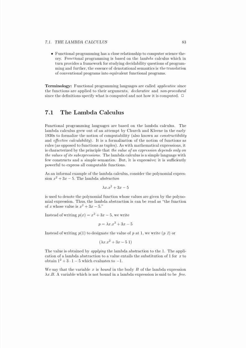
7/3/2019 Theory Introduction to Programming Languages
http://slidepdf.com/reader/full/theory-introduction-to-programming-languages-5584618bb4249 97/233
7.1. THE LAMBDA CALCULUS 83
• Functional programming has a close relationship to computer science the-ory. Functional programming is based on the lambda calculus which inturn provides a framework for studying decidability questions of program-ming and further, the essence of denotational semantics is the translationof conventional programs into equivalent functional programs.
Terminology: Functional programming languages are called applicative sincethe functions are applied to their arguments, declarative and non-procedural since the definitions specify what is computed and not how it is computed. 2
7.1 The Lambda Calculus
Functional programming languages are based on the lambda calculus. Thelambda calculus grew out of an attempt by Church and Kleene in the early1930s to formalize the notion of computability (also known as constructibility and effective calculability ). It is a formalization of the notion of functions asrules (as opposed to functions as tuples). As with mathematical expressions, itis characterized by the principle that the value of an expression depends only on the values of its subexpressions. The lambda calculus is a simple language withfew constructs and a simple semantics. But, it is expressive; it is sufficientlypowerful to express all computable functions.
As an informal example of the lambda calculus, consider the polynomial expres-sion x2 + 3x − 5. The lambda abstraction
λx.x2 + 3x − 5
is used to denote the polynomial function whose values are given by the polyno-mial expression. Thus, the lambda abstraction is can be read as “the functionof x whose value is x2 + 3x − 5.”
Instead of writing p(x) = x2 + 3x − 5, we write
p = λx.x2 + 3x − 5
Instead of writing p(1) to designate the value of p at 1, we write (p 1) or
(λx.x
2
+ 3x − 5 1)
The value is obtained by applying the lambda abstraction to the 1. The appli-cation of a lambda abstraction to a value entails the substitution of 1 for x toobtain 12 + 3 · 1 − 5 which evaluates to −1.
We say that the variable x is bound in the body B of the lambda expressionλx.B. A variable which is not bound in a lambda expression is said to be free.
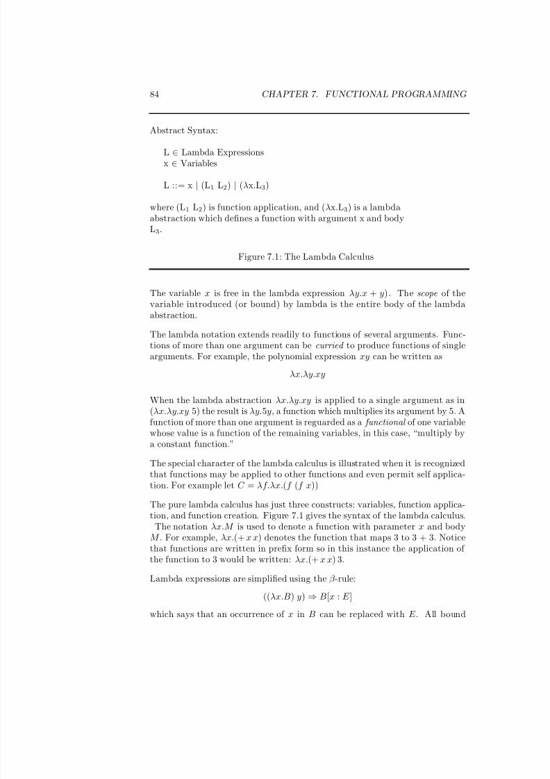
7/3/2019 Theory Introduction to Programming Languages
http://slidepdf.com/reader/full/theory-introduction-to-programming-languages-5584618bb4249 98/233
84 CHAPTER 7. FUNCTIONAL PROGRAMMING
Abstract Syntax:
L ∈ Lambda Expressionsx ∈ Variables
L ::= x | (L1 L2) | (λx.L3)
where (L1 L2) is function application, and (λx.L3) is a lambdaabstraction which defines a function with argument x and bodyL3.
Figure 7.1: The Lambda Calculus
The variable x is free in the lambda expression λy.x + y). The scope of thevariable introduced (or bound) by lambda is the entire body of the lambdaabstraction.
The lambda notation extends readily to functions of several arguments. Func-tions of more than one argument can be curried to produce functions of singlearguments. For example, the polynomial expression xy can be written as
λx.λy.xy
When the lambda abstraction λx.λy.xy is applied to a single argument as in
(λx.λy.xy 5) the result is λy.5y, a function which multiplies its argument by 5. Afunction of more than one argument is reguarded as a functional of one variablewhose value is a function of the remaining variables, in this case, “multiply bya constant function.”
The special character of the lambda calculus is illustrated when it is recognizedthat functions may be applied to other functions and even permit self applica-tion. For example let C = λf.λx.(f (f x))
The pure lambda calculus has just three constructs: variables, function applica-tion, and function creation. Figure 7.1 gives the syntax of the lambda calculus.
The notation λx.M is used to denote a function with parameter x and bodyM . For example, λx.(+ x x) denotes the function that maps 3 to 3 + 3. Notice
that functions are written in prefix form so in this instance the application of the function to 3 would be written: λx.(+ x x) 3.
Lambda expressions are simplified using the β -rule:
((λx.B) y) ⇒ B[x : E ]
which says that an occurrence of x in B can be replaced with E . All bound
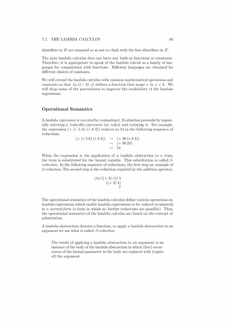
7/3/2019 Theory Introduction to Programming Languages
http://slidepdf.com/reader/full/theory-introduction-to-programming-languages-5584618bb4249 99/233
7.1. THE LAMBDA CALCULUS 85
identifiers in B are renamed so as not to clash with the free identifiers in E .
The pure lambda calculus does not have any built-in functions or constants.Therefore, it is appropriate to speak of the lambda calculi as a family of lan-guages for computation with functions. Different languages are obtained fordifferent choices of constants.
We will extend the lambda calculus with common mathematical operations andconstants so that λx.((+ 3) x) defines a function that maps x to x + 3. Wewill drop some of the parentheses to improve the readability of the lambdaexpressions.
Operational Semantics
A lambda expression is executed by evaluating it. Evaluation proceeds by repeat-edly selecting a reducible expression (or redex ) and reducing it. For example,the expression (+ (∗ 5 6) (∗ 8 3)) reduces to 54 in the following sequence of reductions.
(+ (∗ 5 6) (∗ 8 3)) → (+ 30 (∗ 8 3))→ (+ 30 24)→ 54
When the expression is the application of a lambda abstraction to a term,the term is substituted for the bound variable. This substitution is called β -reduction . In the following sequence of reductions, the first step an example of
β -reduction . The second step is the reduction required by the addition operator.
(λx.((+ 3) x)) 4((+ 3) 4)
7
The operational semantics of the lambda calculus define various operations onlambda expressions which enable lambda expressions to be reduced (evaluated)to a normal form (a form in which no further reductions are possible). Thus,the operational semantics of the lambda calculus are based on the concept of substitution.
A lambda abstraction denotes a function, to apply a lambda abstraction to anargument we use what is called β -reduction .
The result of applying a lambda abstraction to an argument is aninstance of the body of the lambda abstraction in which (free) occur-rences of the formal parameter in the body are replaced with (copiesof) the argument.
7/3/2019 Theory Introduction to Programming Languages
http://slidepdf.com/reader/full/theory-introduction-to-programming-languages-5584618bb4249 100/233
86 CHAPTER 7. FUNCTIONAL PROGRAMMING
The following formula is a formalization of β -reduction .
(λx.B M ) ↔ B[x : M ]
The notation B[x : M ] means the replacement of free occurrences of x in Bwith M .
One problem which arises with β -reduction is the following. Suppose we applyβ -reduction as follows.
(λx.B M ) ↔ B[x : M ]
where y is a free variable in M but y occurs bound in B. Then upon thesubstitution of M for x, y becomes bound. To prevent this from occurring, weneed to do the following.
To prevent free variables from becoming bound requires the replace-ment of free variables with new free variable name, a name whichdoes not occur in B.
This type of replacement is called α-reduction . The following formula is a for-malization of α-reduction ,
λx.B ↔ λy.B[x : y]
where y is not free in B.
Now we define replacement (substitution) as follows:
x[x : M ] = M c[x : M ] = c where c is a variable or constant other than x.(A B )[x : M ] = (A[x : M ] B[x : M ])(λx.B)[x : M ] = (λx.B)(λy.B)[x : M ] = λz.(B[y : z][x : M ]) where z is a new variable name
which does not occur free in B or M .
Figure 7.2 defines the operational semantics of the lambda calculus in terms of β -reduction.
Reduction Order
Given a lambda expression, the previous section provides the tools required toevaluate the expression but, the previous section did not tell us what order weshould use in reducing the lambda expressions.
Church-Rosser Theorem I If E 1 ↔ E 2 then there is an expression E , such thatE 1 → E and E 2 → E .
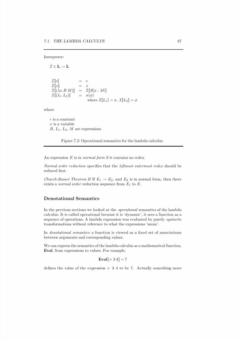
7/3/2019 Theory Introduction to Programming Languages
http://slidepdf.com/reader/full/theory-introduction-to-programming-languages-5584618bb4249 101/233
7.1. THE LAMBDA CALCULUS 87
Interpreter:
I ∈ L → L
I [[c]] = c I [[x]] = x I [[(λx.B M )]] = I [[B[x : M ]]] I [[(L1 L2)]] = σ(φ)
where I [[L1]] = σ, I [[L2]] = φ
where
c is a constantx is a variableB, L1, L2, M are expressions
Figure 7.2: Operational semantics for the lambda calculus
An expression E is in normal form if it contains no redex.
Normal order reduction specifies that the leftmost outermost redex should bereduced first.
Church-Rosser Theorem II If E 1 → E 2, and E 2 is in normal form, then thereexists a normal order reduction sequence from E 1 to E .
Denotational Semantics
In the previous sections we looked at the operational semantics of the lambdacalculus. It is called operational because it is ‘dynamic’, it sees a function as asequence of operations. A lambda expression was evaluated by purely syntactictransformations without reference to what the expressions ‘mean’.
In denotational semantics a function is viewed as a fixed set of associations
between arguments and corresponding values.
We can express the semantics of the lambda calculus as a mathematical function,Eval, from expressions to values. For example,
Eval[[+ 3 4]] = 7
defines the value of the expression + 3 4 to be 7. Actually something more
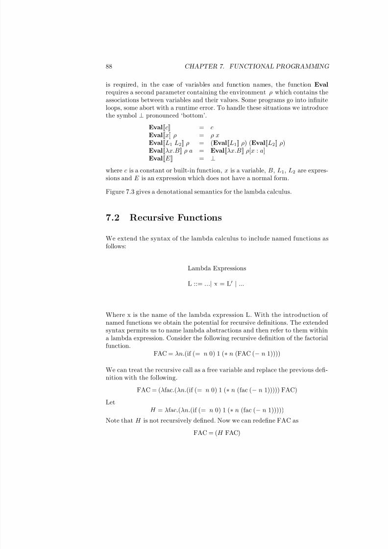
7/3/2019 Theory Introduction to Programming Languages
http://slidepdf.com/reader/full/theory-introduction-to-programming-languages-5584618bb4249 102/233
88 CHAPTER 7. FUNCTIONAL PROGRAMMING
is required, in the case of variables and function names, the function Evalrequires a second parameter containing the environment ρ which contains theassociations between variables and their values. Some programs go into infiniteloops, some abort with a runtime error. To handle these situations we introducethe symbol ⊥ pronounced ‘bottom’.
Eval[[c]] = cEval[[x]] ρ = ρ xEval[[L1 L2]] ρ = (Eval[[L1]] ρ) (Eval[[L2]] ρ)Eval[[λx.B]] ρ a = Eval[[λx.B]] ρ[x : a]Eval[[E ]] = ⊥
where c is a constant or built-in function, x is a variable, B, L1, L2 are expres-sions and E is an expression which does not have a normal form.
Figure 7.3 gives a denotational semantics for the lambda calculus.
7.2 Recursive Functions
We extend the syntax of the lambda calculus to include named functions asfollows:
Lambda Expressions
L ::= ...| x = L | ...
Where x is the name of the lambda expression L. With the introduction of named functions we obtain the potential for recursive definitions. The extendedsyntax permits us to name lambda abstractions and then refer to them withina lambda expression. Consider the following recursive definition of the factorialfunction.
FAC = λn.(if (= n 0) 1 (∗ n (FAC (− n 1))))
We can treat the recursive call as a free variable and replace the previous defi-nition with the following.
FAC = (λfac.(λn.(if (= n 0) 1 (∗ n (fac (− n 1))))) FAC)
LetH = λfac.(λn.(if (= n 0) 1 (∗ n (fac (− n 1)))))
Note that H is not recursively defined. Now we can redefine FAC as
FAC = (H FAC)
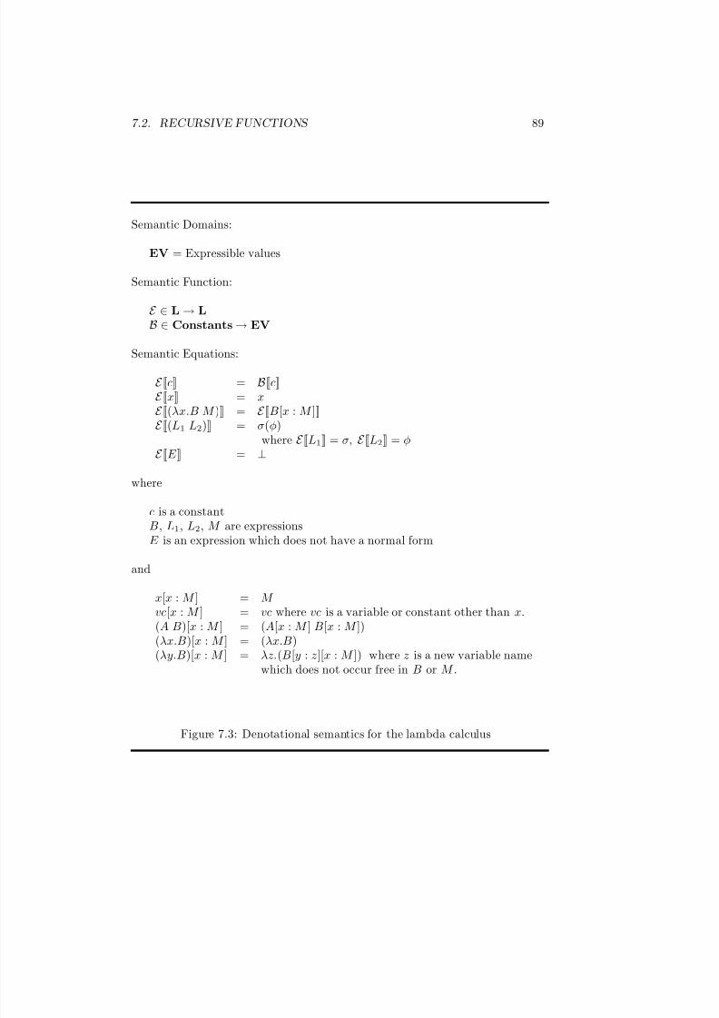
7/3/2019 Theory Introduction to Programming Languages
http://slidepdf.com/reader/full/theory-introduction-to-programming-languages-5584618bb4249 103/233
7.2. RECURSIVE FUNCTIONS 89
Semantic Domains:
EV = Expressible values
Semantic Function:
E ∈ L → LB ∈ Constants → EV
Semantic Equations:
E [[c]] = B[[c]]E [[x]] = xE [[(λx.B M )]] = E [[B[x : M ]]]E [[(L1 L2)]] = σ(φ)
where E [[L1]] = σ, E [[L2]] = φE [[E ]] = ⊥
where
c is a constantB, L1, L2, M are expressionsE is an expression which does not have a normal form
and
x[x : M ] = M vc[x : M ] = vc where vc is a variable or constant other than x.(A B)[x : M ] = (A[x : M ] B[x : M ])(λx.B)[x : M ] = (λx.B)(λy.B)[x : M ] = λz.(B[y : z][x : M ]) where z is a new variable name
which does not occur free in B or M .
Figure 7.3: Denotational semantics for the lambda calculus
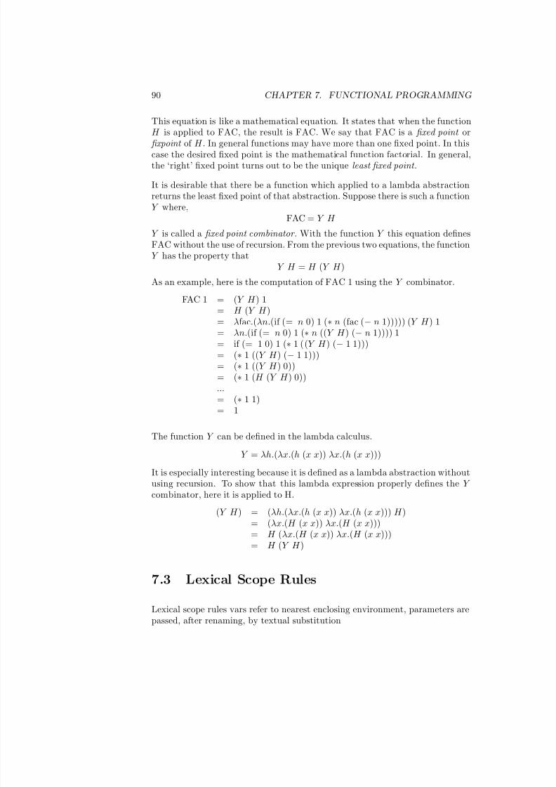
7/3/2019 Theory Introduction to Programming Languages
http://slidepdf.com/reader/full/theory-introduction-to-programming-languages-5584618bb4249 104/233
90 CHAPTER 7. FUNCTIONAL PROGRAMMING
This equation is like a mathematical equation. It states that when the functionH is applied to FAC, the result is FAC. We say that FAC is a fixed point or fixpoint of H . In general functions may have more than one fixed point. In thiscase the desired fixed point is the mathematical function factorial. In general,the ‘right’ fixed point turns out to be the unique least fixed point .
It is desirable that there be a function which applied to a lambda abstractionreturns the least fixed point of that abstraction. Suppose there is such a functionY where,
FAC = Y H
Y is called a fixed point combinator . With the function Y this equation definesFAC without the use of recursion. From the previous two equations, the functionY has the property that
Y H = H (Y H )
As an example, here is the computation of FAC 1 using the Y combinator.
FAC 1 = (Y H ) 1= H (Y H )= λfac.(λn.(if (= n 0) 1 (∗ n (fac (− n 1))))) (Y H ) 1= λn.(if (= n 0) 1 (∗ n ((Y H ) (− n 1)))) 1= if (= 1 0) 1 (∗ 1 ((Y H ) (− 1 1)))= (∗ 1 ((Y H ) (− 1 1)))= (∗ 1 ((Y H ) 0))= (∗ 1 (H (Y H ) 0))...= (∗ 1 1)
= 1
The function Y can be defined in the lambda calculus.
Y = λh.(λx.(h (x x)) λx.(h (x x)))
It is especially interesting because it is defined as a lambda abstraction withoutusing recursion. To show that this lambda expression properly defines the Y combinator, here it is applied to H.
(Y H ) = (λh.(λx.(h (x x)) λx.(h (x x))) H )= (λx.(H (x x)) λx.(H (x x)))= H (λx.(H (x x)) λx.(H (x x)))= H (Y H )
7.3 Lexical Scope Rules
Lexical scope rules vars refer to nearest enclosing environment, parameters arepassed, after renaming, by textual substitution
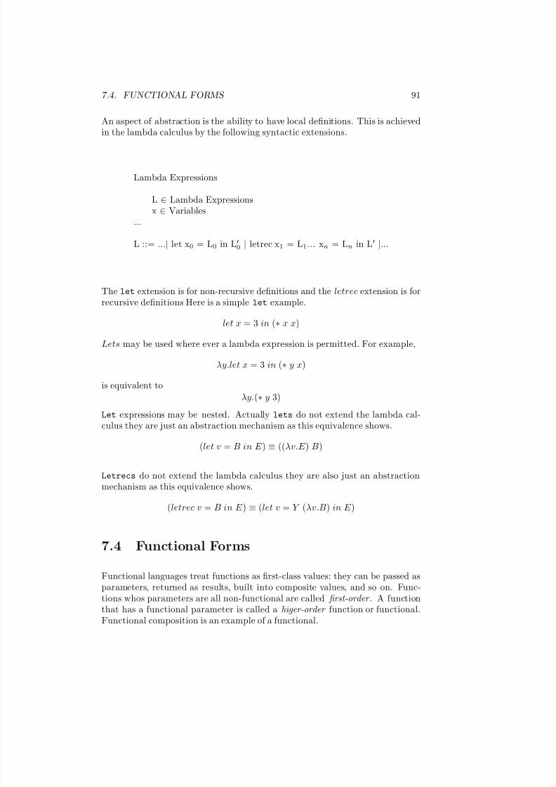
7/3/2019 Theory Introduction to Programming Languages
http://slidepdf.com/reader/full/theory-introduction-to-programming-languages-5584618bb4249 105/233
7.4. FUNCTIONAL FORMS 91
An aspect of abstraction is the ability to have local definitions. This is achievedin the lambda calculus by the following syntactic extensions.
Lambda Expressions
L ∈ Lambda Expressionsx ∈ Variables
...
L ::= ...| let x0 = L0 in L0 | letrec x1 = L1... xn = Ln in L |...
The let extension is for non-recursive definitions and the letrec extension is forrecursive definitions Here is a simple let example.
let x = 3 in (∗ x x)
Lets may be used where ever a lambda expression is permitted. For example,
λy.let x = 3 in (∗ y x)
is equivalent to
λy.(∗ y 3)
Let expressions may be nested. Actually lets do not extend the lambda cal-culus they are just an abstraction mechanism as this equivalence shows.
(let v = B in E ) ≡ ((λv.E ) B)
Letrecs do not extend the lambda calculus they are also just an abstractionmechanism as this equivalence shows.
(letrec v = B in E ) ≡ (let v = Y (λv.B) in E )
7.4 Functional Forms
Functional languages treat functions as first-class values: they can be passed asparameters, returned as results, built into composite values, and so on. Func-tions whos parameters are all non-functional are called first-order . A functionthat has a functional parameter is called a higer-order function or functional.Functional composition is an example of a functional.
7/3/2019 Theory Introduction to Programming Languages
http://slidepdf.com/reader/full/theory-introduction-to-programming-languages-5584618bb4249 106/233
92 CHAPTER 7. FUNCTIONAL PROGRAMMING
double (x) = x * x
quad = double ◦ double
twice (f) = f ◦ f
odd = not ◦ even
Functionals are often used to construct reusable code and to obtain much of thepower of imperative programming within the functional paradigm.
An important functional results from partial application For example, supposethere is the function power defined as follows:
power ( n, b) = if n = 0 then 1 else b*power(n-1, b)
As written power raises a base b to a positive integer power n. The expressionpower(2) is a function of one argument which when applied to a value returnsthe square of the value.
composition f ◦ g (x) = f(g(x))
dispatching f & g (x) = (f(x), g(x))
parallel
currying
apply apply(f,a) = f(a)
iterate iterate(f,n) (a) = f(f(...(f(a))...))
(λ x.λ y.((* x) y) 3 = λy.((* 3) y)
7.5 Evaluation Order
A function is strict if it is sure to need its argument. If a function is non-strict,we say that it is lazy . Why???
parameter passing: by value, by name, and lazy evaluation
Infinite Data Structures
call by need
streams and perpetual processes
7/3/2019 Theory Introduction to Programming Languages
http://slidepdf.com/reader/full/theory-introduction-to-programming-languages-5584618bb4249 107/233
7.6. VALUES AND TYPES 93
A function f is strict if and only if (f ⊥) =⊥
Scheme evaluates its parameters before passing (eliminates need for renaming)a space and time efficiency consideration.
Concurrent evaluation
7.6 Values and Types
Pre-defined Data Types
Integer, Real, Character, Tuples, Lists Enumerations, algebraic types (unions)
7.7 Type Systems and Polymorphism
Pattern matching, Product type, sequences, functions, ML, Miranda
7.8 Program Transformation
Since functional programs consist of function definitions and expression evalua-tions they are suitable for program transformation and formal proof just like anyother mathematical system. It is the principle of referential transparency thatmakes this possible. The basic proof rule is that: identifiers may be replaced by their values.
For example,
f 0 = 1
f n+1 = (n+1)*(f n)
fp 0 fn = fn
fp n+1 in = fp n (n+1)*in
f n = f p n 1
f 0 = f p 0 1 by definition of f and fp
assume f n = f p n 1
7/3/2019 Theory Introduction to Programming Languages
http://slidepdf.com/reader/full/theory-introduction-to-programming-languages-5584618bb4249 108/233
94 CHAPTER 7. FUNCTIONAL PROGRAMMING
show f n+1 = fp n+1 1
f n+1 = (n+1)*f n
= (n+1)*fp n 1
and
k*fp m n = fp m k*n since
1*fp m n = fp m 1*n
and
(k+1)*fp m n = k*fp m n + fp m n = fp m k*n + fp m n
fold
unfold
7.9 Pattern matching
f 0 = 1
f (n+1) = (n+1)*f(n)
insert (item Empty Tree) = BST item Empty Tree Empty Tree
insert (item BST x LST RST) = BST x insert (item LST) RST if item < x
BST x LST insert( item RST ) if item > x
7.10 Combinatorial Logic
The β reduction rule is expensive to implement. It requires the textual substitu-tion of the argument for each occurrence of the parameter and further requiresthat no free variable in the argument should become bound. This has lead tothe study of ways in which variables can be eliminated.
Curry, Feys, and Craig define a number of combinators among them the follow-ing:
S = λf.(λg.(λx.fx(gx)))
K = λx.λy.xI = λx.xY = λf.λx.(f (x x))λx.(f (x x))
These definitions lead to transformation rules for sequences of combinators. Thereduction rules for the SKI calculus are given in Figure 7.4. The reductionrules require that reductions be performed left to right. If no S, K, I, or Yreduction applies, then brackets are removed and reductions continue.

7/3/2019 Theory Introduction to Programming Languages
http://slidepdf.com/reader/full/theory-introduction-to-programming-languages-5584618bb4249 109/233
7.10. COMBINATORIAL LOGIC 95
• S f g x → f x (g x)
• K c x → c
• I x → x
• Y e → e (Y e)
• (A B) → A B
• (A B C)→ A B C
Figure 7.4: Reduction rules for SKI calculus
C[[CV ]] → CV C[[(E 1 E 2)]] → (C[[E 1]] C[[E 2]])C[[λx.E ]] → A[[(x, C[[E ]])]]A[[(x, x)]] → I A[[(x, c)]] → (Kc)A[[(x, (E 1 E 2))]] → ((S A[[(x, E 1)]]) A[[(x, E 2)]])
Where CV is a constant or a variable.
Figure 7.5: Translation rules for the lambda calculus to SKI code
The SKI calculus is computationally complete; that is, these three operationsare sufficient to implement any operation. This is demonstrated by the rules inFigure 7.5 which translate lambda expressions to formulas in the SKI calculus.
Any functional programming language can be implemented by a machine thatimplements the SKI combinators since, functional languages can be transformedinto lambda expressions and thus to SKI formulas.
Function application is relatively expensive on conventional computers. Theprinciple reason is the complexity of maintaining the data structures that sup-port access to the bound identifiers. The problems are especially severe whenhigher-order functions are permitted. Because a formula of the SKI calculuscontains no bound identifiers, its reduction rules can be implemented as simpledata structure manipulations. Further, the reduction rules can be applied in anyorder, or in parallel. Thus it is possible to design massively parallel computers(graph reduction machines) that execute functional languages efficiently.
Recursive functions may be defined with the Y operator.
7/3/2019 Theory Introduction to Programming Languages
http://slidepdf.com/reader/full/theory-introduction-to-programming-languages-5584618bb4249 110/233
96 CHAPTER 7. FUNCTIONAL PROGRAMMING
• S (K e) (K f) → K (e f)
• S (K e) I → e
• S (K e) f → (B e) f
• S e (K f) → (C e) f
The optimizations must be applied in the order given.
Figure 7.6: Optimizations for SKI code
Optimizations
Notice that the size of the SKI code grows quadratically in the number of boundvariables. Figure 7.6 contains a number of optimizations for SKI code. Amongthe optimizations are two additional combinators, the B and C combinators.
Just as machine language (assembler) can be used for programming, combinato-rial logic can be used as a programming language. The programming languageFP is a programming language based on the idea of combinatorial logic.
7.11 Scheme
Scheme, a descendent of LISP, is based on the lambda calculus. Although it hasimperative features, in this section we ignore those features and concentrate onthe lambda calculus like features of Scheme.
Scheme has two kinds of objects, atoms and lists. Atoms are represented bystrings of non-blank characters. A list is represented by a sequence of atomsor lists separated by blanks and enclosed in parentheses. Functions in Schemeare also represented by lists. This facilitates the creation of functions whichcreate other functions. A function can be created by another function and thenthe function applied to a list of arguments. This is an important feature of
languages for AI applications.
Syntax
The syntax of Scheme is similar to that of the lambda calculus.
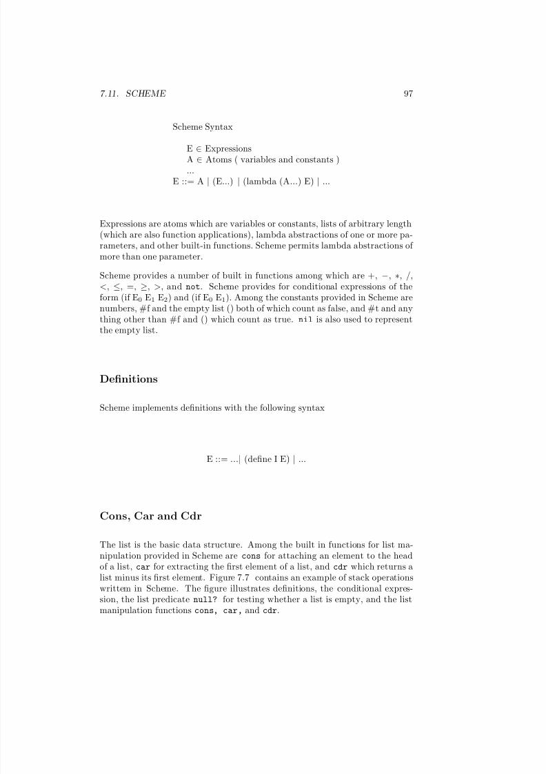
7/3/2019 Theory Introduction to Programming Languages
http://slidepdf.com/reader/full/theory-introduction-to-programming-languages-5584618bb4249 111/233
7.11. SCHEME 97
Scheme Syntax
E ∈ ExpressionsA ∈ Atoms ( variables and constants )...
E ::= A | (E...) | (lambda (A...) E) | ...
Expressions are atoms which are variables or constants, lists of arbitrary length(which are also function applications), lambda abstractions of one or more pa-rameters, and other built-in functions. Scheme permits lambda abstractions of more than one parameter.
Scheme provides a number of built in functions among which are +, −, ∗, /,<, ≤, =, ≥, >, and not. Scheme provides for conditional expressions of theform (if E0 E1 E2) and (if E0 E1). Among the constants provided in Scheme arenumbers, #f and the empty list () both of which count as false, and #t and anything other than #f and () which count as true. nil is also used to representthe empty list.
Definitions
Scheme implements definitions with the following syntax
E ::= ...| (define I E) | ...
Cons, Car and Cdr
The list is the basic data structure. Among the built in functions for list ma-nipulation provided in Scheme are cons for attaching an element to the headof a list, car for extracting the first element of a list, and cdr which returns alist minus its first element. Figure 7.7 contains an example of stack operationswrittem in Scheme. The figure illustrates definitions, the conditional expres-sion, the list predicate null? for testing whether a list is empty, and the listmanipulation functions cons, car, and cdr.
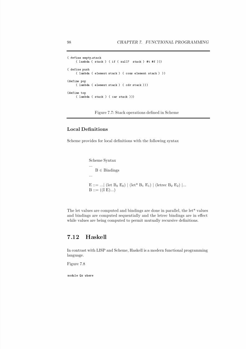
7/3/2019 Theory Introduction to Programming Languages
http://slidepdf.com/reader/full/theory-introduction-to-programming-languages-5584618bb4249 112/233
98 CHAPTER 7. FUNCTIONAL PROGRAMMING
( define empty stack
( lambda ( stack ) ( if ( null? stack ) #t #f )))
( define push( lambda ( element stack ) ( cons element stack ) ))
(define pop( lambda ( element stack ) ( cdr stack )))
(define top
( lambda ( stack ) ( car stack )))
Figure 7.7: Stack operations defined in Scheme
Local Definitions
Scheme provides for local definitions with the following syntax
Scheme Syntax...
B ∈ Bindings...
E ::= ...| (let B0 E0) | (let* B1 E1) | (letrec B2 E2) |...B ::= ((I E)...)
The let values are computed and bindings are done in parallel, the let* valuesand bindings are computed sequentially and the letrec bindings are in effectwhile values are being computed to permit mutually recursive definitions.
7.12 Haskell
In contrast with LISP and Scheme, Haskell is a modern functional programminglanguage.
Figure 7.8
module Qs where

7/3/2019 Theory Introduction to Programming Languages
http://slidepdf.com/reader/full/theory-introduction-to-programming-languages-5584618bb4249 113/233
7.12. HASKELL 99
module AStack( Stack, push, pop, top, size ) where
data Stack a = Empty| MkStack a (Stack a)
push :: a -> Stack a -> Stack apush x s = MkStack x s
size :: Stack a -> Integersize s = length (stkToLst s) where
stkToLst Empty = []
stktoLst (MkStack x s) = x:xs where xs = stkToLst s
pop :: Stack a -> (a, Stack a)
pop (MkStack x s) = (x, case s of r -> i r where i x = x)
top :: Stack a -> a
top (MkStack x s) = x
Figure 7.8: A sample program in Haskell
qs :: [Int] -> [Int]
qs [] = []
qs (a:as) = qs [x | x <- as, x <= a] ++ [a] ++ qs [x | x <- as, x > a]
module Primes where
primes :: [Int]
primes = map head (iterate sieve [2 ..])
sieve :: [Int] -> [Int]
sieve (p:ps) = [x | x <- ps, (x ‘mod‘ p) /= 0]
module Fact where
fact :: Integer -> Integer
fact 0 = 1fact (n+1) = (n+1)*fact n -- * "Foo"
fact _ = error "Negative argument to factorial"
module Pascal where
pascal :: [[Int]]
pascal = [1] : [[x+y | (x,y) <- zip ([0]++r) (r++[0])] | r <- pascal]
tab :: Int -> ShowS
tab 0 = \x -> x
tab (n+1) = showChar ’ ’ . tab n
showRow :: [Int] -> ShowS

7/3/2019 Theory Introduction to Programming Languages
http://slidepdf.com/reader/full/theory-introduction-to-programming-languages-5584618bb4249 114/233
100 CHAPTER 7. FUNCTIONAL PROGRAMMING
showRow [] = showChar ’\n’
showRow (n:ns) = shows n . showChar ’ ’ . showRow ns
showTriangle 1 (t:_) = showRow t
showTriangle (n+1) (t:ts) = tab n . showRow t . showTriangle n ts
module Merge where
merge :: [Int] -> [Int] -> [Int]
merge [] x = x
merge x [] = x merge l1@(a:b) l2@(c:d) = if a < c then a:(merge b l2)
else c:(merge l1 d)
half [] = []half [x] = [x]
half (x:y:z) = x:r where r = half z
sort [] = []
sort [x] = [x]
sort l = merge (sort odds) (sort evens) whereodds = half l
evens = half (tail l)
this
7.13 Discussion and Further Reading
Functional programming languages have been presented in terms of a sequence of virtual machines. Functional programming languages can be translated into thelambda calculus, the lambda calculus into combinatorial logic and combinatoriallogic into the code for a graph reduction machine. All of these are virtualmachines.
Models of the lambda calculus.
History [18] For an easily accessable introduction to functional programming,the lambda calculus, combinators and a graph machine implementation see [25].
For Backus’ Turing Award paper on functional programming see [2]. The com-plete reference for the lambda calculus is [3]. For all you ever wanted to knowabout combinatory logic see [6, 7, 13]. For an introduction to functional pro-gramming see [12, 4, 20]. For an intoduction to LISP see [19] and for commonLISP see [29]. For a through introduction to Scheme see [1]. Haskell On therelationship of the lambda calculus to programming languages see [17]. For theimplementation of functional programming languages see [12, 22].
7/3/2019 Theory Introduction to Programming Languages
http://slidepdf.com/reader/full/theory-introduction-to-programming-languages-5584618bb4249 115/233
7.14. EXERCISES 101
7.14 Exercises
1. Simplify the following expressions to a final (normal ) form, if one exists.If one does not exist, explain why.
(a) ((λx.(x y))(λz.z))
(b) ((λx.((λy.(x y)) x))(λz.w))
(c) ((((λf.(λg.(λx.((f x)(g x)))))(λm.(λn.(n m))))(λn.z)) p)
(d) ((λx.(x x))(λx.(x x)))
(e) ((λf.((λg.((f f ) g))(λh.(k h))))(λy.y)))
(f) (λg.((λf.((λx.(f (x x)))(λx.(f (x x))))) g))
(g) (λx.(λy.((− y) x))) 4 5
(h) ((λf.(f 3))(λx.((+ 1) x)))
2. In addition to the β -rule, the lambda calculus includes the following tworules:
α-rule: (λx.E ) ⇒ (λy.E [x : y])η-rule: (λx.E x) ⇒ E where x does not occur free in E
Redo the previous exercise making use of the η-rule whenever possible.What value is there in the α-rule?
3. The lambda calculus can be used to simulate computation on truth valuesand numbers.
(a) Let true be the name of the lambda expression λx.λy.x and false bethe name of the lambda expression λx.λy.y. Show that ((true E 1) E 2) ⇒E 1 and ((false E 1) E 2) ⇒ E 2. Define lambda expressions not, and,and or that behave like their Boolean operation counterparts.
(b) Let 0 be the name of the lambda expression λx.λy.y, 1 be the nameof the lambda expression λx.λy.(x y), 2 be the name of the lambdaexpression λx.λy.(x (x y)), 3 be the name of the lambda expressionλx.λy.(x; (x (x y))), and so on. Prove that the lambda expressionsucc defined as λz.λx.λy.(x ((z x) y)) rewrites a number to its suc-cessor.
4. Recursively defined functions can also be simulated in the lambda calculus.Let Y be the name of the expression λf.λx.(f (x x))λx.(f (x x))
(a) Show that for any expression E, there exists an expression W suchthat (Y E ) ⇒ (W W ), and that (W W ) ⇒ (E (W W )). Hence,(Y E ) ⇒ E (E (E (...E (W W )...)))
7/3/2019 Theory Introduction to Programming Languages
http://slidepdf.com/reader/full/theory-introduction-to-programming-languages-5584618bb4249 116/233
102 CHAPTER 7. FUNCTIONAL PROGRAMMING
(b) Using the lambda expressions that you defined in the previous partsof this exercise, define a recursive lambda expression add that per-forms addition on the numbers defined earlier, that is, ((add m) n) ⇒m + n.
5. Data constructors can be modeled in the lambda calculus. Let cons =(λa.λb.λf.fab), head = (λc.c(λa.λb.a)) and tail = (λc.c(λa.λb.b)). Showthat
(a) head ( cons a b ) = a
(b) tail ( cons a b ) = b
6. Show that (((S(KK))I)S) is (KS).
7. What is (((SI)I)X) for any formula X?
8. Compile (λx. + x x) to SKI code.
9. Compile λx.(F (x x)) to SKI code.
10. Compile λx.λy.xy to SKI code. Check your answer by reducing both((λx.λy.xy) a b) and the SKI code applied to a b.
11. Apply the optimizations to the SKI code for λx.λy.xy and compare theresult with the unoptimized code.
12. Apply the optimizations to the SKI code for λx.(F (x y)) and λy.(F (x y)).
13. Association lists etc
14. HOF
7/3/2019 Theory Introduction to Programming Languages
http://slidepdf.com/reader/full/theory-introduction-to-programming-languages-5584618bb4249 117/233
Chapter 8
Logic Programming
Logic programming is characterized by programming with relations and infer-ence.
Keywords and phrases: Horn clause, Logic programming, inference, modus po-nens, modus tollens, logic variable, unification, unifier, most general unifier,occurs-check, backtracking, closed world assumption, meta programming, pat-tern matching.
A logic program consists of a set of axioms and a goal statement. The rules of inference are applied to determine whether the axioms are sufficient to ensurethe truth of the goal statement. The execution of a logic program correspondsto the construction of a proof of the goal statement from the axioms.
In the logic programming model the programmer is responsible for specifyingthe basic logical relationships and does not specify the manner in which theinference rules are applied. Thus
Logic + Control = Algorithms
Logic programming is based on tuples. Predicates are abstractions and gener-alization of the data type of tuples. Recall, a tuple is an element of
S 0 × S 1 × ... × S n
103
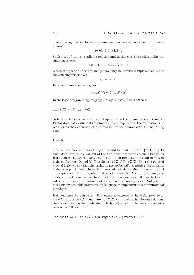
7/3/2019 Theory Introduction to Programming Languages
http://slidepdf.com/reader/full/theory-introduction-to-programming-languages-5584618bb4249 118/233
104 CHAPTER 8. LOGIC PROGRAMMING
The squaring function for natural numbers may be written as a set of tuples asfollows:
{(0, 0), (1, 1), (2, 4)...}
Such a set of tuples is called a relation and in this case the tuples define thesquaring relation.
sqr = {(0, 0), (1, 1), (2, 4)...}
Abstracting to the name sqr and generalizing an individual tuple we can definethe squaring relation as:
sqr = (x, x2)
Parameterizing the name gives:
sqr(X, Y ) ← Y is X ∗ X
In the logic programming language Prolog this would be written as:
sqr(X,Y) ← Y is X*X.
Note that the set of tuples is named sqr and that the parameters are X and Y.Prolog does not evaluate its arguments unless required, so the expression Y isX*X forces the evaluation of X*X and unifies the answer with Y. The Prologcode
P ← Q.
may be read in a number of ways; it could be read P where Q or P if Q. Inthis latter form it is a variant of the first-order predicate calculus known asHorn clause logic. A complete reading of the sqr predicate the point of view of logic is: for every X and Y, Y is the sqr of X if Y is X*X. From the point of view of logic, we say that the variables are universally quantified . Horn clauselogic has a particularly simple inference rule which permits its use as a modelof computation. This computational paradigm is called Logic programming anddeals with relations rather than functions or assignments. It uses facts andrules to represent information and deduction to answer queries. Prolog is themost widely available programming language to implement this computationalparadigm.
Relations may be composed. For example, suppose we have the predicates,male(X), siblingof(X,Y), and parentof(Y,Z) which define the obvious relations,then we can define the predicate uncleof(X,Z) which implements the obviousrelation as follows:
uncleof(X,Z) ← male(X), siblingof(X,Y), parentof(Y,Z).
7/3/2019 Theory Introduction to Programming Languages
http://slidepdf.com/reader/full/theory-introduction-to-programming-languages-5584618bb4249 119/233
8.1. INFERENCE ENGINE 105
The logical reading of this rule is as follows: “for every X,Y and Z, X is the uncleof Z, if X is a male who has a sibling Y which is the parent of Z.” Alternately,“X is the uncle of Z, if X is a male and X is a sibing of Y and Y is a parent of Z.”
The difference between logic programming and functional programming may beillustrated as follows. The logic program
f(X,Y) ← Y = X*3+4
is an abreviation for
∀X, Y (f (X, Y ) ← Y = X ∗ 3 + 4)
which asserts a condition that must hold between the corresponding domain and
range elements of the function. In contrast, a functional definition introduces afunctional object to which functional operations such as functional compositionmay be applied.
8.1 Inference Engine
The control portion of the the equation is provide by an inference engine
whose role is to derive theorems based on the set of axioms provided by theprogrammer. The inference engine uses the operations of resolution andunification to construct proofs.
Resolution says that given the axioms
f i f a0, ..., am.
g if f, b0, ..., bn.
the fact
g i f a0, ..., am, b0, ..., bn.
can be derived.
Unification is the binding of variables. For example
8.2 Syntax
There are just four constructs: constants, variables, function symbols, predicatesymbols, and two logical connectives, the comma (and) and the implication
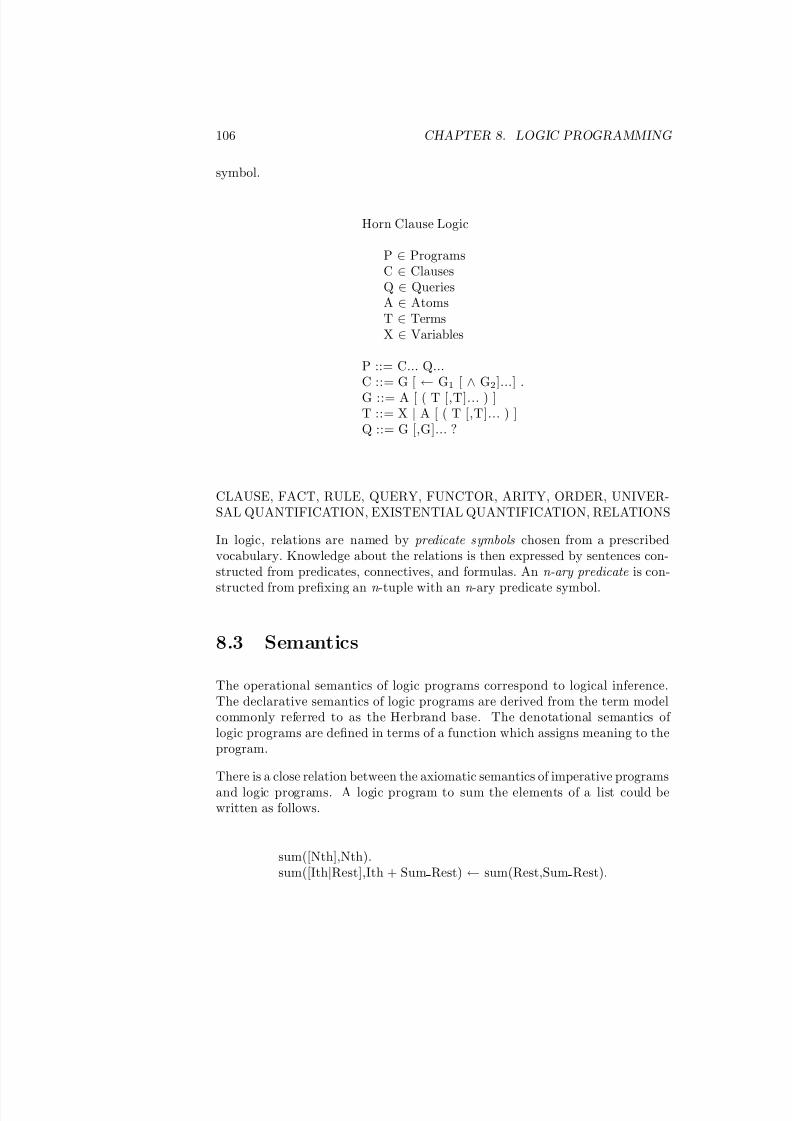
7/3/2019 Theory Introduction to Programming Languages
http://slidepdf.com/reader/full/theory-introduction-to-programming-languages-5584618bb4249 120/233
106 CHAPTER 8. LOGIC PROGRAMMING
symbol.
Horn Clause Logic
P ∈ ProgramsC ∈ ClausesQ ∈ QueriesA ∈ AtomsT ∈ TermsX ∈ Variables
P ::= C... Q...C ::= G [ ← G1 [ ∧ G2]...] .
G ::= A [ ( T [,T]... ) ]T ::= X | A [ ( T [,T]... ) ]Q ::= G [,G]... ?
CLAUSE, FACT, RULE, QUERY, FUNCTOR, ARITY, ORDER, UNIVER-SAL QUANTIFICATION, EXISTENTIAL QUANTIFICATION, RELATIONS
In logic, relations are named by predicate symbols chosen from a prescribedvocabulary. Knowledge about the relations is then expressed by sentences con-structed from predicates, connectives, and formulas. An n-ary predicate is con-
structed from prefixing an n -tuple with an n -ary predicate symbol.
8.3 Semantics
The operational semantics of logic programs correspond to logical inference.The declarative semantics of logic programs are derived from the term modelcommonly referred to as the Herbrand base. The denotational semantics of logic programs are defined in terms of a function which assigns meaning to theprogram.
There is a close relation between the axiomatic semantics of imperative programsand logic programs. A logic program to sum the elements of a list could bewritten as follows.
sum([Nth],Nth).sum([Ith|Rest],Ith + Sum Rest) ← sum(Rest,Sum Rest).

7/3/2019 Theory Introduction to Programming Languages
http://slidepdf.com/reader/full/theory-introduction-to-programming-languages-5584618bb4249 121/233
8.3. SEMANTICS 107
A proof of its correctness is trivial since the logic program is but a statement of the mathematical properties of the sum.
{A[N ] =N
i=N A[i]}
sum([A[N ]], A[N ]).
{N
i=I A[i] = A[I ] + S if 0 < I,N
i=I +1 A[i] = S }
sum([A[I ],...,A[N ]], A[I ] + S ) ← sum([A[I + 1],...,A[N ]], S ).
Operational Semantics
The operational semantics of a logic program can be described in terms of logicalinference using unification and the inference rule resolution . The following logicprogram illustrates logical inference.
a.b ← a.b?
We can conclude b by modus ponens given that b ← a and a. Alternatively, if bis assume to be false then from b ← a and modus tollens we infer ¬ a but sincea is given we have a contradiction and b must hold. The following programillustrates unification.
parent of(a,b).parent of(b,c).ancestor of(Anc,Desc) ← parent of(Anc,Desc).ancestor of(Anc,Desc) ← parent of(Anc,Interm) ∧
ancestor of(Interm,Desc).parent of(a,b)?
ancestor of(a,b)?ancestor of(a,c)?ancestor of(X,Y)?
Consider the query ‘ancestor of(a,b)?’. To answer the question “is a an ancestorof b”, we must select the second rule for the ancestor relation and unify a with
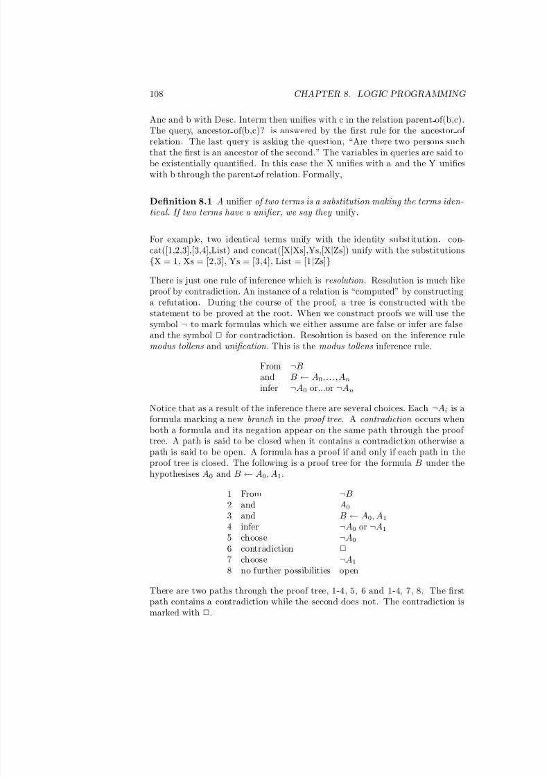
7/3/2019 Theory Introduction to Programming Languages
http://slidepdf.com/reader/full/theory-introduction-to-programming-languages-5584618bb4249 122/233
108 CHAPTER 8. LOGIC PROGRAMMING
Anc and b with Desc. Interm then unifies with c in the relation parent of(b,c).The query, ancestor of(b,c)? is answered by the first rule for the ancestor of relation. The last query is asking the question, “Are there two persons suchthat the first is an ancestor of the second.” The variables in queries are said tobe existentially quantified. In this case the X unifies with a and the Y unifieswith b through the parent of relation. Formally,
Definition 8.1 A unifier of two terms is a substitution making the terms iden-tical. If two terms have a unifier, we say they unify.
For example, two identical terms unify with the identity substitution. con-cat([1,2,3],[3,4],List) and concat([X|Xs],Ys,[X|Zs]) unify with the substitutions{X = 1, Xs = [2,3], Ys = [3,4], List = [1 |Zs]}
There is just one rule of inference which is resolution . Resolution is much likeproof by contradiction. An instance of a relation is “computed” by constructinga refutation. During the course of the proof, a tree is constructed with thestatement to be proved at the root. When we construct proofs we will use thesymbol ¬ to mark formulas which we either assume are false or infer are falseand the symbol 2 for contradiction. Resolution is based on the inference rulemodus tollens and unification . This is the modus tollens inference rule.
From ¬Band B ← A0,...,An
infer ¬A0 or...or ¬An
Notice that as a result of the inference there are several choices. Each ¬Ai is aformula marking a new branch in the proof tree. A contradiction occurs whenboth a formula and its negation appear on the same path through the proof tree. A path is said to be closed when it contains a contradiction otherwise apath is said to be open. A formula has a proof if and only if each path in theproof tree is closed. The following is a proof tree for the formula B under thehypothesises A0 and B ← A0, A1.
1 From ¬B2 and A0
3 and B ← A0, A1
4 infer ¬A0 or ¬A1
5 choose ¬A0
6 contradiction 2
7 choose ¬A1
8 no further possibilities open
There are two paths through the proof tree, 1-4, 5, 6 and 1-4, 7, 8. The firstpath contains a contradiction while the second does not. The contradiction ismarked with 2.
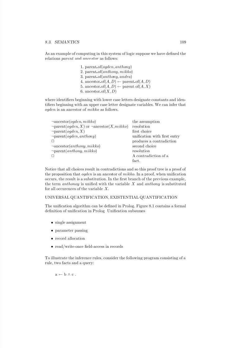
7/3/2019 Theory Introduction to Programming Languages
http://slidepdf.com/reader/full/theory-introduction-to-programming-languages-5584618bb4249 123/233
8.3. SEMANTICS 109
As an example of computing in this system of logic suppose we have defined therelations parent and ancestor as follows:
1. parent of(ogden, anthony)2. parent of(anthony, mikko)3. parent of(anthony, andra)4. ancestor of(A, D) ← parent of(A, D)5. ancestor of(A, D) ← parent of(A, X )6. ancestor of(X, D)
where identifiers beginning with lower case letters designate constants and iden-tifiers beginning with an upper case letter designate variables. We can infer thatogden is an ancestor of mikko as follows.
¬ancestor(ogden, mikko) the assumption¬parent(ogden, X ) or ¬ancestor(X,mikko) resolution¬parent(ogden, X ) first choice¬parent(ogden, anthony) unification with first entry2 produces a contradiction¬ancestor(anthony, mikko) second choice¬parent(anthony, mikko) resolution2 A contradiction of a
fact.
Notice that all choices result in contradictions and so this proof tree is a proof of the proposition that ogden is an ancestor of mikko. In a proof, when unificationoccurs, the result is a substitution. In the first branch of the previous example,
the term anthonoy is unified with the variable X and anthony is substitutedfor all occurences of the variable X .
UNIVERSAL QUANTIFICATION, EXISTENTIAL QUANTIFICATION
The unification algorithm can be defined in Prolog. Figure 8.1 contains a formaldefinition of unification in Prolog Unification subsumes
• single assignment
• parameter passing
• record allocation
• read/write-once field-access in records
To illustrate the inference rules, consider the following program consisting of arule, two facts and a query:
a ← b ∧ c .
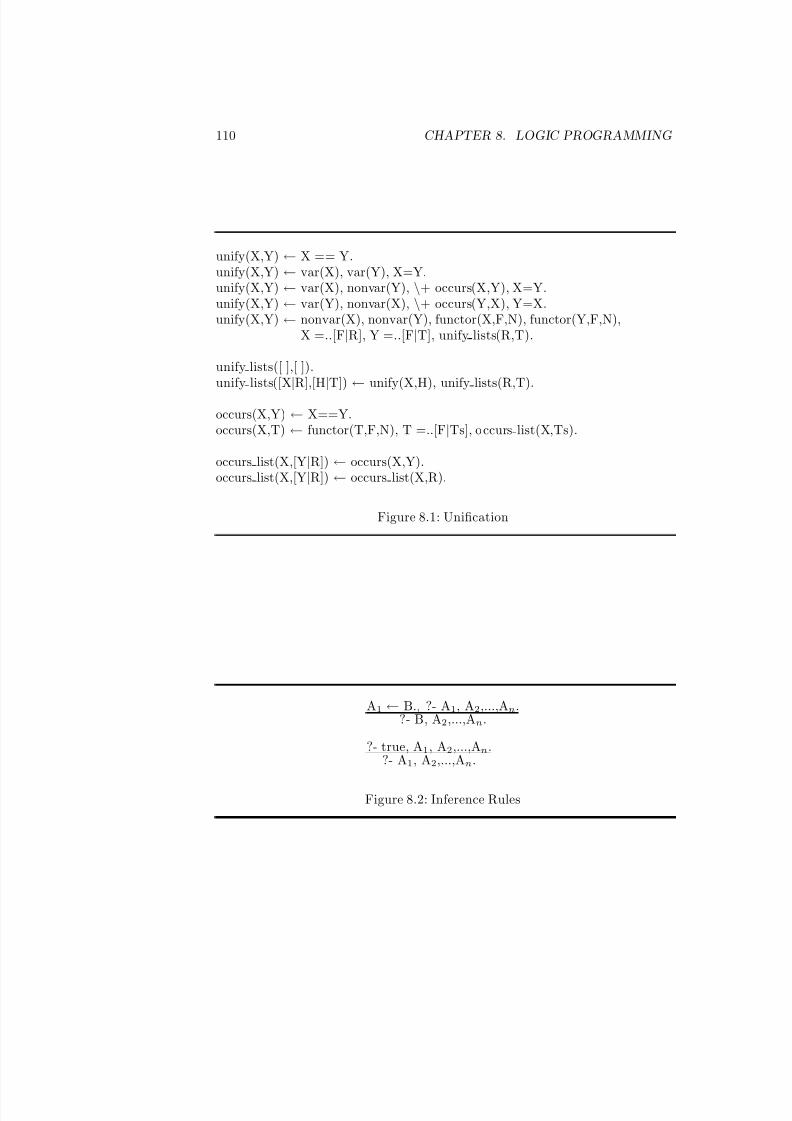
7/3/2019 Theory Introduction to Programming Languages
http://slidepdf.com/reader/full/theory-introduction-to-programming-languages-5584618bb4249 124/233
110 CHAPTER 8. LOGIC PROGRAMMING
unify(X,Y) ← X == Y.unify(X,Y) ← var(X), var(Y), X=Y.unify(X,Y) ← var(X), nonvar(Y), \+ occurs(X,Y), X=Y.unify(X,Y) ← var(Y), nonvar(X), \+ occurs(Y,X), Y=X.unify(X,Y) ← nonvar(X), nonvar(Y), functor(X,F,N), functor(Y,F,N),
X =..[F|R], Y =..[F|T], unify lists(R,T).
unify lists([ ],[ ]).unify lists([X|R],[H|T]) ← unify(X,H), unify lists(R,T).
occurs(X,Y) ← X==Y.occurs(X,T) ← functor(T,F,N), T =..[F|Ts], occurs list(X,Ts).
occurs list(X,[Y|R]) ← occurs(X,Y).occurs list(X,[Y|R]) ← occurs list(X,R).
Figure 8.1: Unification
A1 ← B., ?- A1, A2,...,An.?- B, A2,...,An.
?- true, A1, A2,...,An.?- A1, A2,...,An.
Figure 8.2: Inference Rules
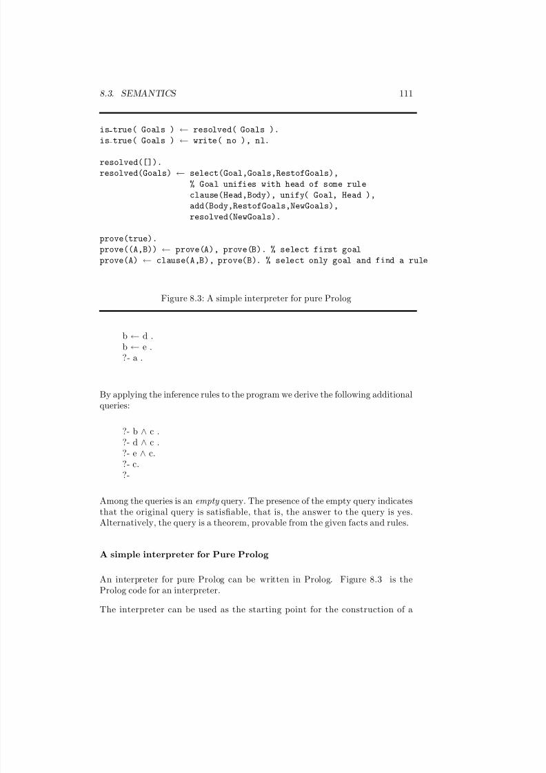
7/3/2019 Theory Introduction to Programming Languages
http://slidepdf.com/reader/full/theory-introduction-to-programming-languages-5584618bb4249 125/233
8.3. SEMANTICS 111
is true( Goals ) ← resolved( Goals ).
is true( Goals ) ← write( no ), nl.
resolved([]).
resolved(Goals) ← select(Goal,Goals,RestofGoals),
% Goal unifies with head of some rule
clause(Head,Body), unify( Goal, Head ),
add(Body,RestofGoals,NewGoals),
resolved(NewGoals).
prove(true).
prove((A,B)) ← prove(A), prove(B). % select first goal
prove(A) ← clause(A,B), prove(B). % select only goal and find a rule
Figure 8.3: A simple interpreter for pure Prolog
b ← d .b ← e .?- a .
By applying the inference rules to the program we derive the following additional
queries:
?- b ∧ c .?- d ∧ c .?- e ∧ c.?- c.?-
Among the queries is an empty query. The presence of the empty query indicatesthat the original query is satisfiable, that is, the answer to the query is yes.Alternatively, the query is a theorem, provable from the given facts and rules.
A simple interpreter for Pure Prolog
An interpreter for pure Prolog can be written in Prolog. Figure 8.3 is theProlog code for an interpreter.
The interpreter can be used as the starting point for the construction of a
7/3/2019 Theory Introduction to Programming Languages
http://slidepdf.com/reader/full/theory-introduction-to-programming-languages-5584618bb4249 126/233
112 CHAPTER 8. LOGIC PROGRAMMING
debugger for Prolog programs and a starting point for the construction of aninference engine for an expert system.
The operational semantics for Prolog are given in Figure 8.4
Declarative Semantics
The declarative semantics of logic programs is based on the standard model-theoretic semantics of first-order logic.
Definition 8.2 Let P be a logic program. The Herbrand universe of P , denoted by U (P ) is the set of ground terms that can be formed from the constants and
function symbols appearing in P
Definition 8.3 The Herbrand base, denoted by B(P ), is the set of all ground goals that can be formed from the predicates in P and the terms in the Herbrand universe.
The Herbrand base is infinite if the Herbrand universe is.
Definition 8.4 An interpretation for a logic program is a subset of the Her-brand base.
An interpretation assigns truth and falsity to the elements of the Herbrand base.A goal in the Herbrand base is true with respect to an interpretation if it is amember of it, false otherwise.
Definition 8.5 An interpretation I is a model for a logic program if for each ground instance of a clause in the program A ← B1,...,Bn A is in I if B1,...,Bn
are in I.
This approach to the semantics is often called the term model .
Denotational Semantics
Denotational semantics assignes meanings to programs based on associatingwith the program a function over the domain computed by the program. Themeaning of the program is defined as the least fixed point 0f the function, if itexists.
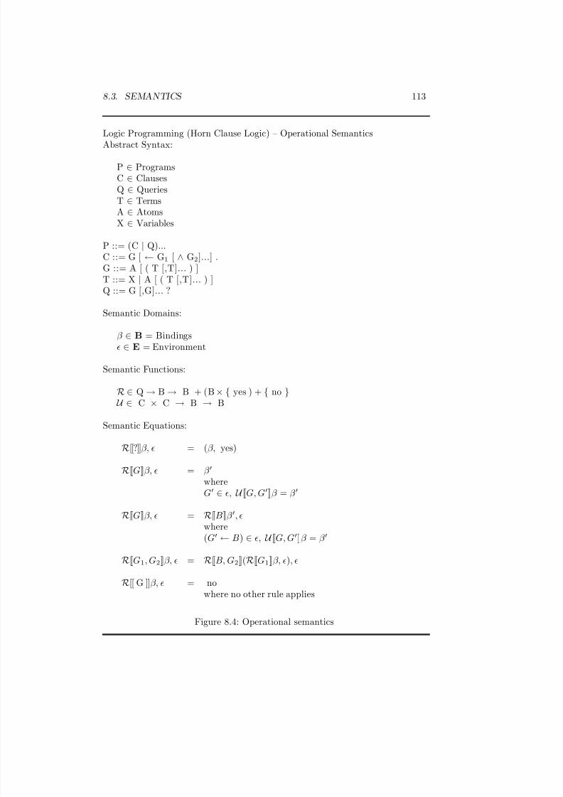
7/3/2019 Theory Introduction to Programming Languages
http://slidepdf.com/reader/full/theory-introduction-to-programming-languages-5584618bb4249 127/233
8.3. SEMANTICS 113
Logic Programming (Horn Clause Logic) – Operational SemanticsAbstract Syntax:
P ∈ ProgramsC ∈ ClausesQ ∈ QueriesT ∈ TermsA ∈ AtomsX ∈ Variables
P ::= (C | Q)...C ::= G [ ← G1 [ ∧ G2]...] .G ::= A [ ( T [,T]... ) ]
T ::= X | A [ ( T [,T]... ) ]Q ::= G [,G]... ?
Semantic Domains:
β ∈ B = Bindings ∈ E = Environment
Semantic Functions:
R ∈ Q → B → B + (B × { yes ) + { no } U ∈ C × C → B → B
Semantic Equations:
R[[?]]β, = (β, yes)
R[[G]]β, = β
whereG ∈ , U [[G, G]]β = β
R[[G]]β, = R[[B]]β , where(G ← B) ∈ , U [[G, G]]β = β
R[[G1, G2]]β, = R[[B, G2]](R[[G1]]β, ),
R[[ G ]]β, = nowhere no other rule applies
Figure 8.4: Operational semantics
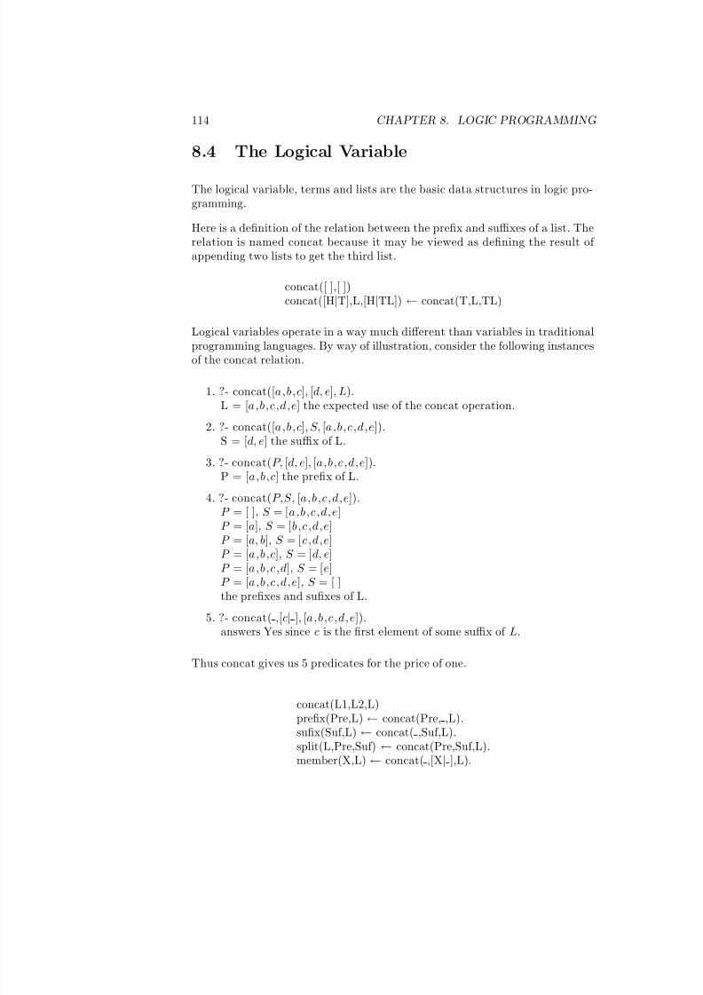
7/3/2019 Theory Introduction to Programming Languages
http://slidepdf.com/reader/full/theory-introduction-to-programming-languages-5584618bb4249 128/233
114 CHAPTER 8. LOGIC PROGRAMMING
8.4 The Logical Variable
The logical variable, terms and lists are the basic data structures in logic pro-gramming.
Here is a definition of the relation between the prefix and suffixes of a list. Therelation is named concat because it may be viewed as defining the result of appending two lists to get the third list.
concat([ ],[ ])concat([H|T],L,[H|TL]) ← concat(T,L,TL)
Logical variables operate in a way much different than variables in traditional
programming languages. By way of illustration, consider the following instancesof the concat relation.
1. ?- concat([a,b,c], [d, e], L).L = [a,b,c,d,e] the expected use of the concat operation.
2. ?- concat([a,b,c], S, [a,b,c,d,e]).S = [d, e] the suffix of L.
3. ?- concat(P, [d, e], [a,b,c,d,e]).P = [a,b,c] the prefix of L.
4. ?- concat(P,S, [a,b,c,d,e]).P = [ ], S = [a,b,c,d,e]
P = [a], S = [b,c,d,e]P = [a, b], S = [c,d,e]P = [a,b,c], S = [d, e]P = [a,b,c,d], S = [e]P = [a,b,c,d,e], S = [ ]the prefixes and sufixes of L.
5. ?- concat( ,[c| ], [a,b,c,d,e]).answers Yes since c is the first element of some suffix of L.
Thus concat gives us 5 predicates for the price of one.
concat(L1,L2,L)prefix(Pre,L) ← concat(Pre, ,L).sufix(Suf,L) ← concat( ,Suf,L).split(L,Pre,Suf) ← concat(Pre,Suf,L).member(X,L) ← concat( ,[X| ],L).
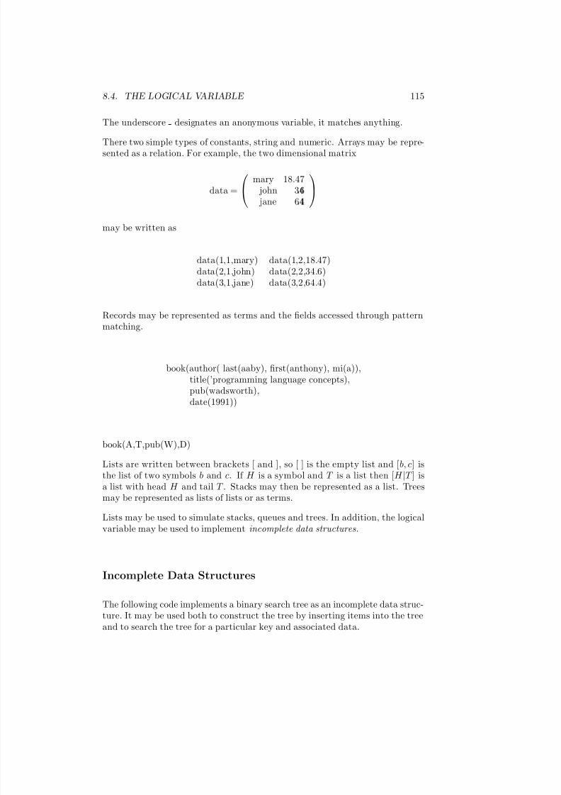
7/3/2019 Theory Introduction to Programming Languages
http://slidepdf.com/reader/full/theory-introduction-to-programming-languages-5584618bb4249 129/233
8.4. THE LOGICAL VARIABLE 115
The underscore designates an anonymous variable, it matches anything.
There two simple types of constants, string and numeric. Arrays may be repre-sented as a relation. For example, the two dimensional matrix
data =
mary 18.47
john 34.6 jane 64.4
may be written as
data(1,1,mary) data(1,2,18.47)data(2,1,john) data(2,2,34.6)data(3,1,jane) data(3,2,64.4)
Records may be represented as terms and the fields accessed through patternmatching.
book(author( last(aaby), first(anthony), mi(a)),title(’programming language concepts),pub(wadsworth),date(1991))
book(A,T,pub(W),D)
Lists are written between brackets [ and ], so [ ] is the empty list and [b, c] isthe list of two symbols b and c. If H is a symbol and T is a list then [H |T ] isa list with head H and tail T . Stacks may then be represented as a list. Treesmay be represented as lists of lists or as terms.
Lists may be used to simulate stacks, queues and trees. In addition, the logicalvariable may be used to implement incomplete data structures.
Incomplete Data Structures
The following code implements a binary search tree as an incomplete data struc-ture. It may be used both to construct the tree by inserting items into the treeand to search the tree for a particular key and associated data.
7/3/2019 Theory Introduction to Programming Languages
http://slidepdf.com/reader/full/theory-introduction-to-programming-languages-5584618bb4249 130/233
116 CHAPTER 8. LOGIC PROGRAMMING
lookup(Key,Data,bt(Key,Data,LT,RT))
lookup(Key,Data,bt(Key0,Data0,LT,RT)) ← Key @< Key0,lookup(Key,Data,LT)
lookup(Key,Data,bt(Key0,Data0,LT,RT)) ← Key @> Key0,lookup(Key,Data,RT)
This is a sequence of calls. Note that the initial call is with the variable BT .
lookup(john,46,BT), lookup(jane,35,BT), lookup(allen,49,BT), lookup(jane,Age,BT).
The first three calls initialize the dictionary to contain those entries while thelast call extracts janes’s age from the dictionary.
The logical and the incomplete data structure can be used to append lists inconstant time. The programming technique is known as difference lists. Theempty difference list is X/X . The concat relation for difference lists is definedas follows:
concat dl(Xs/Ys, Ys/Zs, Xs/Zs)
Here is an example of a use of the definition.
?- concat_dl([1,2,3|X]/X,[4,5,6|Y]/Y,Z).
_X = [4,5,6 | _11]_Y = _11
_Z = [1,2,3,4,5,6 | _11] / _11
Yes
The relation between ordinary lists and difference lists is defined as follows:
ol dl([ ],X/X) ← var(X)ol dl([F|R],[F|DL]/Y) ← ol dl(R,DL/Y)
Arithmetic
Terms are simply patterns they may not have a value in and of themselves.For example, here is a definition of the relation between two numbers and theirproduct.
times(X,Y,X×Y)

7/3/2019 Theory Introduction to Programming Languages
http://slidepdf.com/reader/full/theory-introduction-to-programming-languages-5584618bb4249 131/233
8.5. ITERATION VS RECURSION 117
However, the product is a pattern rather than a value. In order to force theevaluation of an expression, a Prolog definition of the same relation would bewritten
times(X,Y,Z) ← Z is X×Y
8.5 Iteration vs Recursion
Not all recursive definitions require the runtime support usually associated withrecursive subprogram calls. Consider the following elegant mathematical defi-nition of the factorial function.
n! =
1 if n = 0n × (n − 1)! if n > 0
Here is a direct restatement of the definition in a relational form.
factorial(0,1)factorial(N,N×F) ← factorial(N-1,F)
In Prolog this definition does not evaluate either of the expressions N-1 or N×Fthus the value 0 will not occur. To force evaluation of the expressions we rewritethe definition as follows.
factorial(0,1)
factorial(N,F)← M is N-1, factorial(M,Fm), F is N×Fm
Note that in this last version, the call to the factorial predicate is not the lastcall on the right-hand side of the definition. When the last call on the right-hand side is a recursive call (tail recursion ) then the definition is said to be aniterative definition. An iterative version of the factorial relation may be definedusing an accumulator and tail recursion.
fac(N,F) ← fac(N,1,F)fac(0,F,F)fac(N,P,F) ← NP is N×P, M is N-1, fac(M,NP,F)
In this definition, there are two different f ac relations, the first is a 2-ary rela-tion, and the second is a 3-ary relation.
As a further example of the relation between recursive and iterative definitions,here is a recursive version of the relation between a list and its reverse.
reverse([ ], [ ])reverse([H |T ], R) ← reverse(T , T r), concat(T r, [H ], R)
7/3/2019 Theory Introduction to Programming Languages
http://slidepdf.com/reader/full/theory-introduction-to-programming-languages-5584618bb4249 132/233
118 CHAPTER 8. LOGIC PROGRAMMING
and here is an iterative version.
rev(L, R) ← rev(L, [ ], R)rev([ ], R , R)rev([H |T ], L , R) ← rev(T, [H |L], R)
Efficient implementation of recursion is possible when the recursion is tail re-cursion. Tail recursion is implementable as iteration provided no backtrackingmay be required (the only other predicate in the body are builtin predicates).
8.6 Backtracking
When there are multiple clauses defining a relation it is possible that either someof the clauses defining the relation are not applicable in a particular instance orthat there are multiple solutions. The selection of alternate paths during theconstruction of a proof tree is called backtracking .
8.7 Exceptions
Logic programming provides an unusually simple method for handling exceptionconditions. Exceptions are handled by backtracking.
8.8 Prolog = Logic Programming
Prolog is not logic programming. The execution model for Prolog omits the oc-curs check, searches the rules sequentially, and selects goals sequentially. Back-tracking, infinite search trees ...
While there is no standard syntax for Prolog, most implementations recognizethe syntax given in Figure 8.5.
As in functional programming, lists are an important data structure logic pro-gramming. The empty list is represented by [ ], a list of n elements by [X 1,...,X n]and the first i elements of a list and the rest of the list by [ X 1,...,X i|R]. Inaddition, data structures of arbitrary complexity may be constructed from theterms.
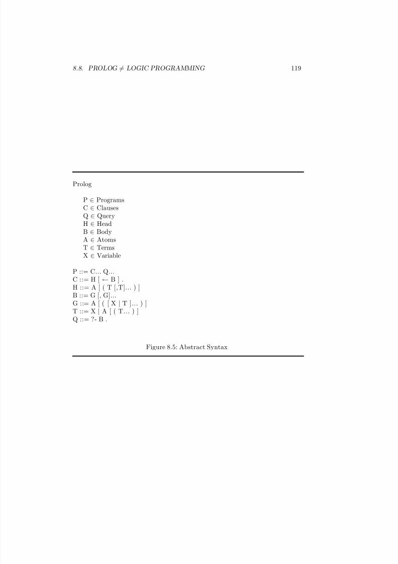
7/3/2019 Theory Introduction to Programming Languages
http://slidepdf.com/reader/full/theory-introduction-to-programming-languages-5584618bb4249 133/233
8.8. PROLOG = LOGIC PROGRAMMING 119
Prolog
P ∈ ProgramsC ∈ ClausesQ ∈ QueryH ∈ HeadB ∈ BodyA ∈ AtomsT ∈ TermsX ∈ Variable
P ::= C... Q...C ::= H [ ← B ] .H ::= A [ ( T [,T]... ) ]
B ::= G [, G]...G ::= A [ ( [ X | T ]... ) ]T ::= X | A [ ( T... ) ]Q ::= ?- B .
Figure 8.5: Abstract Syntax

7/3/2019 Theory Introduction to Programming Languages
http://slidepdf.com/reader/full/theory-introduction-to-programming-languages-5584618bb4249 134/233
120 CHAPTER 8. LOGIC PROGRAMMING
Incompleteness
Incompleteness occurs when there is a solution but it cannot be found. Thedepth first search of Prolog will never answer the query in the following logicprogram.
p( a, b ).p( c, b ).p( X, Z ) ← p( X, Y ), p( Y, Z).p( X, Y ) ← p( Y, X ).?- p( a, c ).
The result is an infinite loop. The first and fourth clauses imply p( b, c ). Thefirst and third clauses with the p( b, c) imply the query. Prolog gets lost in aninfinite branch no matter how the clauses are ordered, how the literals in thebodies are ordered or what search rule with a fixed order for trying the clausesis used. Thus logical completeness requires a breadth-first search which is tooinefficient to be practical.
Unfairness
Unfairness occurs when a permissible value cannot be found.
concat( [ ], L, L ).concat( [H|L1], L2, [X|L] ) ← concat( L1, L2, L ).concat3( L1, L2, L3, L ) ← concat( L1, L2, L12 ),
concat( L12, L3 L ).?- concat3( X, Y, [2], L).
Result is that X is always [ ]. Prologs depth-first search prevents it from finding
other values.
Unsoundness
Unsoundness occurs when there is a successful computation of a goal which isnot a logical consequence of the logic program.

7/3/2019 Theory Introduction to Programming Languages
http://slidepdf.com/reader/full/theory-introduction-to-programming-languages-5584618bb4249 135/233
8.8. PROLOG = LOGIC PROGRAMMING 121
test ← p( X, X ).
p( Y, f( Y )).?- test.
Lacking the occur check Prolog will succeed but test is not a logical consequenceof the logic program.
The execution of this logic program results in the construction of an infinitedata structure.
concat( [ ], L, L ).concat( [H|L1], L2, [X|L] ) ← concat( L1, L2, L ).?- concat( [ ], L, [1|L] ).
In this instance Prolog will succeed (with some trouble printing the answer).There are two solutions, the first is to change the logic and permit infinite terms,the second is to introduce the occur check with the resulting loss of efficiency.
Negation
Negative information cannot be expressed in Horn clause logic. However, Prologprovides the negation operator not and defines negation as failure to find a proof.
p( a ).r( b ) ← not p( Y ).?- not p(b).
The goal succeeds but is not a logical consequence of the logic program.
q( a ) ← r( a ).q( a ) ← not r( a ).r( X ) ← r( f( X ) ).?- q ( a ).
7/3/2019 Theory Introduction to Programming Languages
http://slidepdf.com/reader/full/theory-introduction-to-programming-languages-5584618bb4249 136/233
122 CHAPTER 8. LOGIC PROGRAMMING
The query is a logical consequence of the first two clauses but Prolog cannotdetermine that fact and enters an infinite derivation tree. However the closedworld assumption is useful from a pragmatic point of view.
Control Information
Cut (!): prunes the proof tree.
a(1).a(2).a(3).
p ← a(I),!,print(I),nl,fail.?- p.1
No
Extralogical Features
Input and output introduce side effects.
The extralogical primitives bagof, setof, assert, and retract are outside thescope of first-order logic but are useful from the pragmatic point of view.
In Prolog there are builtin predicates to test for the various syntactic types,lists, numbers, atoms, clauses. Some predicates which are commonly availableare the following.
var(X) X is a variableatomic(A) A is an atom or a numeric constantfunctor(P,F,N) P is an N-ary predicate with functor Fclause(Head,Body) Head ← Body is a formula.
L =..List, call(C), assert(C), retract(C),
bagof(X,P,B), setof(X,P,B)
Figure 8.6 contains an example of meta programming. The code implementsa facility for tracing the execution of a Prolog program. To trace a Prologprogram, instead of entering ?- P. enter ?- trace(P).

7/3/2019 Theory Introduction to Programming Languages
http://slidepdf.com/reader/full/theory-introduction-to-programming-languages-5584618bb4249 137/233
8.8. PROLOG = LOGIC PROGRAMMING 123
trace(Q) ← trace1([Q])trace1([])trace1([true|R]) ← !, trace1(R).trace1([fail|R]) ← !, print(’< ’), print(fail), nl, fail.trace1([B|R]) ← B =..[’,’|BL], !, concat(BL,R,NR), trace1(NR).trace1([F|R]) ← builtin(F),
print(’> ’), print([F|R]), nl,F,trace1(R),print(’<’), print(F), nl
trace1([F|R]) ← clause(F,B),print(’>’), print([F|R]),nl,trace1([B|R]),
print(’< ’), print(F), nltrace1([F|R]) ← \+ builtin(F), \+ clause(F,B),
print(’> ’), print([F|R]),nl,print(’< ’), print(F), print(’ ’), print(fail), nl, fail
Figure 8.6: Program tracer for Prolog
Multidirectionality
Computation of the inverse function must be restricted for efficiency and unde-cidability reasons. For example consider the query
?- factorial(N,5678).
An implementation must either generate and test possible values for N (whichis much too inefficient) or if there is no such N the undecidability of first-orderlogic implies that termination may not occur.
Rule Order
Rule order affects the order of search and thus the shape of the proof tree. Inthe following program
7/3/2019 Theory Introduction to Programming Languages
http://slidepdf.com/reader/full/theory-introduction-to-programming-languages-5584618bb4249 138/233
124 CHAPTER 8. LOGIC PROGRAMMING
concat([ ],L,L).
concat([H|T],L,[H|R]) ← concat(T,L,R).?- concat(L1,[2],L).
the query results in the sequence of answers.
L1 = [ ], L = [2]L1 = [V1], L = [V1,2]L1 = [V1,V2], L = [V1,V2,2]
...
However, if the order of the rules defining concat are interchanged,
concat([H|T],L,[H|R]) ← concat(T,L,R).concat([ ],L,L).?- concat(L1,[2],L).
then the execution fails to terminate, entering an infinite loop since the firstrule is always applicable.
8.9 Database query languages
The query languages of relational database management systems is anotherapproach to the logic model.
The fundamental entity in a relational database is a relation which is viewedas a table of rows and columns, where each row, called a tuple, is an objectand each column is an attribute or propery of the object.
A database consists of one or more relations. The data stored in the relations ismanipulated using commands written in a query language. The operationsprovided the query language include union, set difference, cartesian product,projection, and selection.
7/3/2019 Theory Introduction to Programming Languages
http://slidepdf.com/reader/full/theory-introduction-to-programming-languages-5584618bb4249 139/233
8.10. LOGIC PROGRAMMING VS FUNCTIONAL PROGRAMMING 125
8.10 Logic Programming vs Functional Program-
ming
Functional composition vs composition of relations, backtracking, type checking
8.11 Further Reading
HistoryKowalski’s paper[16]Logic programming techniquesImplementation of Prolog
SQLDCG
8.12 Exercises
1. Modify concat to include an explicit occurs check.
2. Construct a family data base f db(f,m,c,sex) and define the following re-lations, f of, m of, son of, dau of, gf, gm, aunt, uncle, ancestor, half sis,half bro.
3. Business Data base
4. Blocks World
5. CS Degree requirements; course(dept,name,prereq). don’t forget w1 andw2 requirements.
6. Circuit analysis
7. Tail recursion
8. Compiler
9. Interpreter
10. Tic-Tac-Toe11. DCG
12. Construct Prolog analogues of the relational operators for union, set dif-ference, cartesian product, projection and selection.
13. Airline reservation system

7/3/2019 Theory Introduction to Programming Languages
http://slidepdf.com/reader/full/theory-introduction-to-programming-languages-5584618bb4249 140/233
126 CHAPTER 8. LOGIC PROGRAMMING
7/3/2019 Theory Introduction to Programming Languages
http://slidepdf.com/reader/full/theory-introduction-to-programming-languages-5584618bb4249 141/233
Chapter 9
Imperative Programming
Imperative programming is characterized by programming with a state and com-mands which modify the state.
Imperative: a command or order
Procedure: a) the act, method or manner of proceeding in some process or courseof action b) a particular course of action or way of doing something.
Keywords and phrases: Assignment, goto, structured programming, command,statement, procedure, control-flow, imperative language, assertions, axiomaticsemantics. state, variables, instructions, control structures.
Imperative programming languages are characterized by sequences of bindings.Programs are sequences of bindings (state changes) in which a name may bebound an object at one point in the program and later bound to a differentobject. Since the order of the bindings affects the value of expressions, one of theprime issue in the imperative paradigm is control over the sequence of bindings.
These bindings are commands which are issued to a machine. The machine maynot be an actual machine but a virtual machine. Thus, it is common to refer tothe Pascal machine or the Ada machine. The virtual machine provides accessto the hardware through the compiler and the operating system.
In the context of imperative programming languages, a state is more than justthe association between variables and values. It also includes the location of
127
7/3/2019 Theory Introduction to Programming Languages
http://slidepdf.com/reader/full/theory-introduction-to-programming-languages-5584618bb4249 142/233
128 CHAPTER 9. IMPERATIVE PROGRAMMING
control in the program. A portion of code cannot be understood by examiningits constituent parts. The reason is that during the execution of the code, controlmay be transferred to an arbitrary point outside of the code. Thus, the wholeprogram may need to be examined in order to understand a small portion of code.
The imperative programming paradigm is an abstraction of real computerswhich in turn are based on Turing machines and the Von Neumann Machinewith its registers and memory. At the heart of each is the concept of a modifi-able store. Variables and assignment are the programming language analog of the modifiable store. Thus memory is the object that is manipulated and im-perative programming languages provide a variety of commands to manipulatememory.
9.1 Variables and Assignmentassignables–arrays recordsetc
In imperative programming, a variable is a name that may be assigned toa value and later reassigned to a value. The collection of variables and theassociated values constitute the state. The state is a logical model of storagewhich is an association between memory locations and values. Aside: Avariable is not a storage cell, nor is it a name of a storage cell; it is the nameof a value. Most descriptions of imperative programming languages are tied tohardware and implementation considerations where (name, variable, value) =(address, storage cell, bit pattern). Thus, a name is tied to two bindings, a
binding to a location and to a value. The location is called the l-value and thevalue is called the r-value. The necessity for this distinction follows from theimplementation of the assignment where in the assignment, X := X+2, the X onthe left of the assignment denotes a location while the X on the right hand sidedenotes the value.
A variable may be bound to a hardware location at various times. It maybe bound at compile time (rarely), at load time (for languages with static al-location) or at run time (for languages with dynamic allocation). From theimplementation point of view, variable declarations are used to determine theamount of storage required by the program. 2
The following examples illustrate the general form for variable declarations in
imperative programming languages.
Modula-2: variable V of type T
var V : T;
// C: variable V of type T
T V;

7/3/2019 Theory Introduction to Programming Languages
http://slidepdf.com/reader/full/theory-introduction-to-programming-languages-5584618bb4249 143/233
9.1. VARIABLES AND ASSIGNMENT 129
A variable is bound to a value by an assignment. Binding of a variable V tothe value of an expression E.
−−Ada
V := E;
Modula-2
V := E;
//C
V = E ;
APL
V ←
; Scheme (setq V E)
Aside: The use of the symbol (=) in C confuses the distinction betweendefinition, equality and assignment. The symbol (=) is used in mathematics intwo distinct ways. It is used to define and to assert the equality between twovalues. In C it neither means define nor equality. In C the symbol (==) is usedfor equality, while the form: Type Variable is used for definitions. 2
The assignment command is what distinguishes imperative programming lan-guages from other programming languages. The assignment typically has theform: ‘V := E’. The command is read “assign the name V to the value of theexpression E until the name V is reassigned to another value”. The assignmentbinds a name to a value. Aside: The word “assign” is used in accordancewith its English meaning; a name is assigned to an object, not the reverse. Thisis in contrast to the usual programming usage in which a value assigned to avariable. 2
The assignment is not the same as a constant definition because it permitsredefinition. For example, the two assignments:
X := 3;
X := X + 1
are understood as follows: assign X to three and then reassign X to the value of the expression X+1 which is four. Thus, after the sequence of assignments, thevalue of X is four.
Several kinds of assignments are possible. Because of the frequent occurence of assignments of the form: X := X <op> E Algol-68 and C provide an alternativenotation of the form: X <op> := E. A multiple assignment of the form: V0:= V1 := ... := Vn := E causes several names to be assigned to the samevalue. This form of the assignment is found in Algol-60 and in C. A simultaneousassignment of the form: V0,...,Vn := E0,...,En causes several assignments of

7/3/2019 Theory Introduction to Programming Languages
http://slidepdf.com/reader/full/theory-introduction-to-programming-languages-5584618bb4249 144/233
130 CHAPTER 9. IMPERATIVE PROGRAMMING
names to values to occur simultaneously. The simultaneous assignment permitsthe swapping of values without the explicit use of an auxiliary variable.
From the point of view of axiomatic semantics, the assignment the a predicatetransformer. It is a function from predicates to predicates. From the pointof view of denotational semantics, the assignment is a function from states tostates. From the point of view of operational semantics, the assignment changesthe state of an abstract machine.
9.2 Control Structures
Since the assignment can assign names to new values, the order in which as-
signments are executed is important. Control structures are syntactic structuresthat allow assignments to be combined in useful ways.
Terminology: Imperative programming languages often call assignments andcontrol structures commands, statements or instructions. In ordinary English,a statement is an expression of some fact or idea and thus is an inappropriatedesignation. Commands and instructions refer to an action to be performedby a computer. Lacking a more neutral term we will use command to refer toassignments, skip, and control structures. 2
Terminology: Imperative programming is also called procedural programming.In either case the implication is clear. Programs are directions or orders forperforming an action. 2
In addition to the simple assignment, imperative programming languages pro-vide a rich assortment of sequence control mechanisms. Three types of com-mands are required for sequence control: composition , alternation and iteration .
Composition. Composition is usually indicated by placing commands in textualsequence and when it is necessary to determine the syntactic termination pointof a command either line separation or a special symbol (such as the semicolon)is used. Operationally the ordering describes the order or sequence in which theelements are to be executed. At a more abstract level, composition of commandsis indicated by using a composition operator such as the semicolon (C0;C1). InPL/1 and C the semicolon is used as a terminator rather than as a compositionoperator.
Selection: Selection permits the specification of a sequence of commands bycases. The selection of a particular sequence is based on the value of an ex-pression. The if and case commands are the most common representatives of alternation.
7/3/2019 Theory Introduction to Programming Languages
http://slidepdf.com/reader/full/theory-introduction-to-programming-languages-5584618bb4249 145/233
9.2. CONTROL STRUCTURES 131
Iteration: A sequence of commands may be executed zero or more times. Atrun time the sequence is repeatedly composed with itself. There is an expres-sion which whose value at run time determines the number of compositions.The while, repeat and for commands are the most common representative of iteration.
Abstraction: A sequence of commmands may be named and the name used toinvoke the sequence of commands.
Skips
The simplest kind of command is the skip command. It has no effect.
Procedure Calls/Coroutines
A procedure is an abstraction of a sequence of commands. The procedurecall is a reference to the abstraction. The semantics of the procedure call isdetermined by the semantics of the procedure body.
Parameters and arguments
Parameter passing
in, out, in/out, name
Composition
The most common sequence is the sequential composition of two or (more)commands (often written ‘S0;S1’). Sequential composition is available in everyimperative programming language.
Alternation
An alternative command may contain a number of alternative sequences of commands, from which exactly one is chosen to be executed.
Conditional execution discussion: if-then-else, case/switch
-- Ada

7/3/2019 Theory Introduction to Programming Languages
http://slidepdf.com/reader/full/theory-introduction-to-programming-languages-5584618bb4249 146/233
132 CHAPTER 9. IMPERATIVE PROGRAMMING
if condition then
commands
{ elsif condition then
commands }[ else
commands]endif
case expression is
when choice {| choice} => commands
{when choice {| choice} => commands}[when others => commands]
end case;
Often the case command is extended to include an alternative for unspecifiedcases.
case <selector expression> of
...
<value> : <command>;
...
otherwise <command>
end
Iteration
An iterative command has a body which is to be executed repeatedly andhas an expression which determine when the execution will cease.
Loop discussion: while, repeat, for, escapes
[ loop name: ][ iteration scheme ]loop
commands
end loop [ loop name ]
[ loop name: ]while condition loop
commands
end loop [ loop name ]
[ loop name: ]for identifier in [ reverse ] descrete range loop
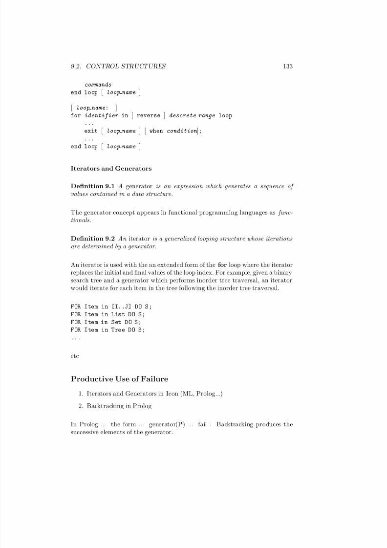
7/3/2019 Theory Introduction to Programming Languages
http://slidepdf.com/reader/full/theory-introduction-to-programming-languages-5584618bb4249 147/233
9.2. CONTROL STRUCTURES 133
commands
end loop [ loop name ]
[ loop name: ]for identifier in [ reverse ] descrete range loop
...
exit [ loop name ] [ when condition ];...
end loop [ loop name ]
Iterators and Generators
Definition 9.1 A generator is an expression which generates a sequence of
values contained in a data structure.
The generator concept appears in functional programming languages as func-tionals.
Definition 9.2 An iterator is a generalized looping structure whose iterationsare determined by a generator.
An iterator is used with the an extended form of the for loop where the iteratorreplaces the initial and final values of the loop index. For example, given a binarysearch tree and a generator which performs inorder tree traversal, an iterator
would iterate for each item in the tree following the inorder tree traversal.
FOR Item in [I..J] DO S;
FOR Item in List DO S;
FOR Item in Set DO S;
FOR Item in Tree DO S;
...
etc
Productive Use of Failure
1. Iterators and Generators in Icon (ML, Prolog...)
2. Backtracking in Prolog
In Prolog ... the form ... generator(P) ... fail . Backtracking produces thesuccessive elements of the generator.
7/3/2019 Theory Introduction to Programming Languages
http://slidepdf.com/reader/full/theory-introduction-to-programming-languages-5584618bb4249 148/233
134 CHAPTER 9. IMPERATIVE PROGRAMMING
% Generators
% Natural Numbers
nat(0).
nat(N) :- nat(M), N is M + 1.
% Infinite sequence from I
inf(I,I).
inf(I,N) :- I1 is I+1, inf(I1,N).
% An Alternate definition of natural numbers (more efficient)
alt_nat(N) :- inf(0,N).
% Sequence of Squares
square(N) :- alt_nat(X), N is X*X.
% Infinite Arithmetic Series
inf(I,J,I) :- I =< J.
inf(I,J,N) :- I < J, I1 is J + (J-I), inf(J,I1,N).
inf(I,J,I) :- I > J.
inf(I,J,N) :- I > J, I1 is J + (J-I), inf(J,I1,N).
% Finite Arithmetic Sequences
% Numbers between I and J increment by 1
between(I,J,I) :- I =< J.
between(I,J,N) :- I < J, I1 is I+1, between(I1,J,N).
between(I,J,I) :- I > J.
between(I,J,N) :- I > J, I1 is I-1, between(I1,J,N).
% Numbers between I and K increment by (J-I)
between(I,J,K,I) :- I =< K.between(I,J,K,N) :- I < K, J1 is J + (J-I), between(J,J1,K,N).
between(I,J,K,I) :- I > K.
between(I,J,K,N) :- I > K, J1 is J + (J-I), between(J,J1,K,N).
% Infinite List -- Arithmetic Series the Prefixes
7/3/2019 Theory Introduction to Programming Languages
http://slidepdf.com/reader/full/theory-introduction-to-programming-languages-5584618bb4249 149/233
9.3. SEQUENCERS 135
inflist(N,[N]).
inflist(N,[N|L]) :- N1 is N+1, inflist(N1,L).
% Primes -- using the sieve
prime(N) :- primes(PL), last(PL,N).
% List of Primes
primes(PL) :- inflist(2,L2), sieve(L2,PL).
sieve([],[]).
sieve([P|L],[P|IDL]) :- sieveP(P,L,PL), sieve(PL,IDL).
sieveP(P,[],[]).sieveP(P,[N|L],[N|IDL]) :- N mod P > 0, sieveP(P,L,IDL).
sieveP(P,[N|L], IDL) :- N mod P =:= 0, L \= [], sieveP(P,L,IDL).
last([N],N).
last([H|T],N) :- last(T,N).
% Primes -- using the sieve (no list)
sprime(N) :- inflist(2,L2), ssieve(L2,N).
ssieve([P],P).
ssieve([P|L],NP) :- L \= [], sieveP(P,L,PL), ssieve(PL,NP).
% B-Tree Generator -- Inorder traversal (Order important)
traverse(btree(Item,LB,RB),I) :- traverse(LB,I).
traverse(btree(Item,LB,RB),Item).
traverse(btree(Item,LB,RB),I) :- traverse(RB,I).
9.3 Sequencers
There are several common features of imperative programming languages thattend to make reasoning about the program difficult. The goto command [9]breaks the sequential continuity of the program. When when the use of thegoto command is undisciplined the breaks involve abrupt shifts of context.
In Ada, the exit sequencer terminates an enclosing loop. All enclosing loopsupto and including the named loop are exited and execution follows with thecommand following the named loop.
7/3/2019 Theory Introduction to Programming Languages
http://slidepdf.com/reader/full/theory-introduction-to-programming-languages-5584618bb4249 150/233
136 CHAPTER 9. IMPERATIVE PROGRAMMING
Ada uses the return sequencer to terminate the execution of the body of aprocedure or function and in the case of a function, to return the result of thecomputation.
Exception handers are sequencers that take control when an exception is raised.
A sequencer is a construct that allows more general control flows to be pro-grammed.
• Jumps
• Exits
• Exceptions – propagation, raising, resumption, handler (implicit invoca-tion)
• Coroutines
The machine languge of a typical computer includes instructions which allow anyinstruction to be selected as the next instruction. A sequencer is a construct thatis provided to give high-level programming languages some of this flexibilty. Weconsider three sequencers, jumps, escapes, and exceptions. The most powerfulsequencer (the goto) is also the most criticized. Sequencers can make it difficultto understand a program by producing ‘spaghetti’ like code. So named becausethe control seems to wander around in the code like the strands of spaghetti.
9.4 Jumps
A jump is an explicit transfer of control from one point in a progam to anotherprogram point. Jumps come in unconditional and conditional forms:
goto L
if conditional expression goto L
At the machine level alternation and iteration may be implmented using labelsand goto commands. Goto commands often take two forms:
1. Unconditional goto. The unconditional goto command has the form:
goto LABELi
The sequence of instructions next executed begin with the command la-beled with LABELi.
7/3/2019 Theory Introduction to Programming Languages
http://slidepdf.com/reader/full/theory-introduction-to-programming-languages-5584618bb4249 151/233
9.5. ESCAPE 137
2. Conditional goto. The conditional goto command has the form:
if conditional expression then goto LABELi
If the conditional expression is true then execution transfers to the se-quence of commands headed by the command labeled with LABELi other-wise it continues with the command following the conditional goto.
The goto commands have a number of advantages, they have direct hardwaresupport and are completely general purpose. There are also a number of disad-vantages, programs are flat without hierarchical structure and the code may bedifficult to read and understand.
The term structured programming was coined to describe a style of programmingthat emphasizes hierarchical program structures in which each command has oneentry point and one exit point.
9.5 Escape
An escape is a sequence which terminates the execution of a textually enclosingconstruct.
An escape of the form:
return expr
is often used to exit a function call and return the value computed by thefunction.
An escape of the form:
exit(n)
is used to exit n enclosing constructs. The exit command can be used in con- junction with a general loop command to produce while and repeat as well asmore general looping constructs.
In C a break command sends control out of the enclosing loop to the com-mand following the loop while the continue command transfers control to thebeginning of the enclosing loop.

7/3/2019 Theory Introduction to Programming Languages
http://slidepdf.com/reader/full/theory-introduction-to-programming-languages-5584618bb4249 152/233
138 CHAPTER 9. IMPERATIVE PROGRAMMING
9.6 Exceptions
There are many “exception” conditions that can arise in program execution.Some exception conditions are normal for example, the end of an input filemarks the end of the input phase of a program. Other exception conditionsare genuine errors for example, division by zero. Exception handlers of variousforms can be found in PL/1, ML, CLU, Ada, Scheme and other languages.
There are two basic types of exceptions which arise during program execution.They are domain failure, and range failure.
Domain failure occurs when the input parameters of an operation do notsatisfy the requirements of the operation. For example, end of file on a
read instruction, division by zero.
Range failure occurs when an operation is unable to produce a result forvalues which are in the range. For example, division by numbers withinan of zero.
Definition 9.3 An exception condition is a condition that prevents the com-pletion of an operation. The recognition of the exception is called raising theexception.
Once an exception is raised it must be handled. Handling exceptions is impor-tant for the constuction of robust programs. A program is said to be robust if it
recovers from exceptional conditions.
Definition 9.4 The action to resolve the exception is called handling the ex-ception. The propagation of an exception is the passing of the exception to thecontext where it can be handled.
The simplest method of handling exceptions is to ignore it and continue execu-tion with the next instruction. This prevents programmer from learning aboutthe exception and may lead to erroneous results.
The most common method of handling exceptions is to abort execution. Thisis not exceptable for file I/O but may be acceptable for an array index beingout of bounds or for division by zero.
The next level of error handling is to return a value outside the range of theoperation. This could be a global variable, a result parameter or a functionresult. This approach requires explicit checking by the programmer for theerror values. For example, the eof boolean is set to true when the programhas read the last item in a file. The eof condition can then be checked before
7/3/2019 Theory Introduction to Programming Languages
http://slidepdf.com/reader/full/theory-introduction-to-programming-languages-5584618bb4249 153/233
9.6. EXCEPTIONS 139
attempting to read from a file. The disadvantage of this approach is that aprogram tends to get cluttered with code to test the results. A more seriousconsequence is that a programmer may forget to include a test with the resultthat the exception is ignored.
Responses to an Exception
Return a label and execute a goto – Fortran
Issues
Resumption of Program Execution
Once an exception has been detected, control is passed to the handler that de-fines the action to be taken when the exception is raised. The question remains,what happens after handling the exception?
One approach is to treat exception handlers as subroutines to which controlis passed and after the execution of the handler control returns to the pointfollowing the call to the handler. This is the approach taken in PL/1. It impliesthat the handler “fixed” the state that raised the condition.
Another approach is that the exception handler’s function is to provide a clean-up operation prior to termination. This is the approach taken in Ada. The
unit in which the exception occured terminates and control passes to the callingunit. Exceptions are propagated until an exception handler is found.
Suppression of the Exception
Some exceptions are inefficient to implement (for example, run time range checkson array bounds). The such exceptions are usually implemented in softwareand may require considerable implementation overhead. Some languages givethe programmer control over whether such checks and the raising of the cor-responding exception will be performed. This permits the checks to be turnedon during program development and testing and then turned off for normal
execution.
1. Handler Specification
2. Default Handlers
3. Propagation of Exception
7/3/2019 Theory Introduction to Programming Languages
http://slidepdf.com/reader/full/theory-introduction-to-programming-languages-5584618bb4249 154/233
140 CHAPTER 9. IMPERATIVE PROGRAMMING
Productive Use of Failure
Prolog, Icon
9.7 Coroutines
Multiple threads of control but control is passed from thread to thread underthe active thread’s control.
9.8 Processes
Multiple threads of control where each thread may be active concurrently.
9.9 Side effects
At the root of differences between mathematical notations and imperative pro-grams is the notion of referential transparency (substitutivity of equals forequals). Manipulation of formulas in algebra, arithmetic, and logic rely onthe principle of referential transparency. Imperative programming languages
violate the principle. For example:
function f(x:integer) : integer;
begin y := y+1; f := y + x end
This “function” in addition to computing a value also changes the value of the global variable y. This change to a global variable is called a side effect . Inaddition to modifying a global variable, it is difficult to reason with the functionitself. If at some point in the program it is known that y = z = 0 then f(z) =
1 in the sense that after the call f(z) will return 1. But, should the followingexpression occur in the program,
1 + f(z) = f(z) + f(z)
it will be false.
As another example of side effects, consider the C function getint as used in thefollowing two expressions.
7/3/2019 Theory Introduction to Programming Languages
http://slidepdf.com/reader/full/theory-introduction-to-programming-languages-5584618bb4249 155/233
9.10. ALIASING 141
2 * getint ()
getint () + getint ()
The two expressions are different. The first multiplies the next integer readfrom the input file by two while the second expression denotes the sum of thenext two successive integers read from the input file. And yet as mathematicalexpressions they should denote the same value.
Side effects are a feature of imperative programming languages that make rea-soning about the program difficult. Side effects are used to provide communi-cation among program units. When undisciplined access to global variables ispermitted, the program becomes difficult to understand. The entire programmust be scanned to determine which program units access and modify the globalvariables since the call command does not reveal what variables may be affected
by the call.
9.10 Aliasing
Two variables are aliases if they denote (share) the same data object duringa unit activation. Aliasing is another feature of imperative programming lan-guages that makes programs harder to understand and harder to reason about.
The following assignments appear to be independent of each other.
x := a + b
y := c + d
But suppose x and c are aliases for the same object. In this case, the assign-ments are interdependent and the order of evaluation is important. Often inthe optimization of code it is desireable to reorder steps or to delete unecessarysteps. This cannot be done when aliasing is possible.
Aliasing can occur in several ways.
The purpose of the equivalence command in FORTRAN is the creation of aliases.It permits the efficient use of memory (historically a scarce commodity) and canbe used as a crude form of a variant record.
When a data object is passed by “reference” it is referenced both by its name inthe calling environment and its parameter name in the called environment. An-other way in which aliasing can occur is when a data object may be a componentof several data objects (referenced through pointer linkages).
Aliasing can arise from variable definitions and from variable parameters. Con-sider calls confuse( i, i) and confuse( a[i], a[j] ) given the following
7/3/2019 Theory Introduction to Programming Languages
http://slidepdf.com/reader/full/theory-introduction-to-programming-languages-5584618bb4249 156/233
142 CHAPTER 9. IMPERATIVE PROGRAMMING
Pascal procedure
procedure confuse (var m, n : integer);
begin n := 1; n := m + n end
in the first call i is set to 2. The result of the second call depends on the valuesof i and j. The second call shows that the detection of aliasing may be delayeduntil run time. No compiler can detect aliasing in general.
• Formal and actual parameters share the same data object.
• Procedure calls have overlapping actual parameters.
• A formal parameter and a global variable denote the same data object.
Pointers are intrinsically generators of aliasing.
var p , q : ↑ T ;
...
new(p);
q : = p
Dangling References
type pointer = ^ Integer
var p : Pointer;
procedure Dangling;
var q : Pointer;
begin;new(q); q^ := 23; p := q; dispose(q)
end;
beginnew(p); Dangling(p)
end;
The pointer p is left pointing to a non-existent value.
The problem of aliasing arises as soon as a language supports variables andassignment. If more than one assignment is permitted on the same variable x ,the fact that x=a cannot be used at any other point in the program to infer a

7/3/2019 Theory Introduction to Programming Languages
http://slidepdf.com/reader/full/theory-introduction-to-programming-languages-5584618bb4249 157/233
9.11. REASONING ABOUT IMPERATIVE PROGRAMS 143
property of x from a property of a . Aliasing and global variables only magnifythe issue.
Imperative constructs jeopardize many of the fundamental techniques for rea-soning about mathematical objects. Much of the work on the theory of program-ming languages is an attempt to explain the “referentially opaque” features of programming languages in terms of well-defined mathematical constructs.
9.11 Reasoning about Imperative Programs
Imperative constructs jeopardize many of the fundamental techniques for rea-soning about mathematical objects. For example, the assignment axiom of axiomatic semantics is valid only for languages without aliasing and side effects.Much of the work on the theory of programming languages is an attempt toexplain the “referentially opaque” features of programming languages in termsof well-defined mathematical constructs. By providing descriptions of program-ming language features in terms of standard mathematical concepts, program-ming language theory makes it possible to manipulate programs and reasonabout them using precise and rigorous techniques. Unfortunately, the resultingdescriptions are complex and the notational machinery is difficult to use in allbut small examples. It is this complexity that provides a strong motivativationto provide functional and logic programming as alternatives to the imperativeprogramming paradigm.
9.12 Expressions with side effects
Most imperative programming languges permit expressions to have side effects.
9.13 Sequential Expressions
Imperative programming languages with their emphasis on the sequential evalu-
ation of commands often fail to provide a similar sequentiality to the evaluationof expressions. The following code illustrates a common programming situationwhere there are two or more conditions which must remain true for iteration tooccur.
i := 1;
while (i <= length) and (list[i] <> value) do i := i+1

7/3/2019 Theory Introduction to Programming Languages
http://slidepdf.com/reader/full/theory-introduction-to-programming-languages-5584618bb4249 158/233
144 CHAPTER 9. IMPERATIVE PROGRAMMING
command := |IDENT := exp|label : command
| GOTO label| IF boo exp THEN GOTO label| command; command
Figure 9.1: A set of structured commands
command := SKIP
| IDENT := exp
| IF guarded command alternative ... FI| DO guarded command alternative ... OD
| command ; command
guarded command := guard → command
alternative := [] guarded command
Figure 9.2: A set of structured commands
The code implements a sequential search for a value in a table and terminateswhen either the entire table has been searched or the value is found. Assumingthat the subscript range for list is 1 to length it seems reasonable that thetermination of the loop should occur either when the index is out of bounds orwhen the value is found. That is, the arguments to the and should be evaluatedsequentually and if the first argument is false the remaining argument need notbe evaluated since the value of the expression cannot be true. Such an evaluationscheme is call short-circuit evaluation.
In most implementations, if the value is in the list, the program aborts with asubscript out of range error.
The Ada language provides the special operators and then and or else so thatthe programmer can specify short-circuit evaluation.
9.14 Structured Programming
Given the imporatance of sequence control, it is not suprizing that considerableeffort has been given to finding appropriate control structures. Figure 9.1 givesa set of basic control structures. Figure 9.2 gives a set of structured commands.
7/3/2019 Theory Introduction to Programming Languages
http://slidepdf.com/reader/full/theory-introduction-to-programming-languages-5584618bb4249 159/233
9.15. EXPRESSION-ORIENTED LANGUAGES 145
9.15 Expression-oriented languages
An expression-oriented language is an imperative languge in which distinctionsbetween expressions and commands are eliminated. This permits a simplifi-cation in the syntax in that the language does not need both procedure andfunction abstraction nor conditional expressions and commands since he evalu-ation of an expression may both yield a value and have a side effect of updatingvariables. The assignment V : = E can be defined to yield the value of the ex-pression E and assign V to the value of E. Since the assignment is an expression,expressions of the form V0 := ... := (Vn := E) are possible giving multipleassigment for free. The assignment returns the 0-tuple () in ML.
The value of E0;E1 the value of E1. E0 is evaluated for its side-effect and thevalue is discarded. There is no obvious result for iterative control structures.Typically they are defined to return zero or a null value.
Expression-oriented languages achieve simplicity and regularity by eliminatingthe distinction between expressions and commands. Often this can result inan opaque programming style. Algol-68, Scheme, ML and C are examples of expression oriented languages.
9.16 Further Reading
Exercises1. Give all possible forms of assignment found in the programming language
C.
2. Give axiomatic, denotational and operational semantics for the simulta-neous assignment. What is the effect on the semantic descriptions if ex-pressions are permitted to have side effects?
3. Ambiguity of Pascal’s if command.
4. Compare the case command of Ada to the switch command of C++.
5. Compare the looping constructs of Ada and C++
6. Alternative control structures
7. Goto elimination
8. Axiomatic semantics
9. Denotational semantics
7/3/2019 Theory Introduction to Programming Languages
http://slidepdf.com/reader/full/theory-introduction-to-programming-languages-5584618bb4249 160/233
146 CHAPTER 9. IMPERATIVE PROGRAMMING
10. Operational semantics
11. Provide implementations of the alternative and iterative control structuresin terms of labels and gotos.
12. Classify the following common error/exception conditions as either domainor range errors.
(a) overflow – value exceeds representational capabilities
(b) undefined value – variable value is undefined
(c) subscript error – array subscript out of range
(d) end of input – attempt to read past end of input file
(e) data error – data of the wrong type
7/3/2019 Theory Introduction to Programming Languages
http://slidepdf.com/reader/full/theory-introduction-to-programming-languages-5584618bb4249 161/233
Chapter 10
Concurrent Programming
Concurrent programming is characterized by programming with more than oneprocess.
Keywords and phrases Pipelines, parallel processes, message passing, monitors,concurrent programming, safety, liveness, deadlock, livelock, fairness, commu-nication, synchronization producer-consumer, dining philosophers.
Operations are sequential , if they occur one after the other, ordered in time.Operations are concurrent , if they overlap in time. Operations in the sourcetext of a program are concurrent if they could be, but need not be, executedin parallel. Concurrent programming involves the notations for expressing po-tential parallelism and the techniques for solving the resulting synchronizationand communication problems. Notations for explicit concurrency are a pro-gram structuring technique while parallelism is mode of execution provided bythe underlying hardware. Thus we can have parallel execution without explicitconcurrency in the language. This is the case when functional and logic pro-
gramming languages are executed on appropriate hardware or a program iscompiled by a parallelizing compiler. We can have concurrency in a languagewithout parallel execution. This is the case when a program (with or withoutexplicit concurrent sections) is executed on a single processor. In this case, theprogram is executed by interleaving executions of concurrent operations in thesource text.
147

7/3/2019 Theory Introduction to Programming Languages
http://slidepdf.com/reader/full/theory-introduction-to-programming-languages-5584618bb4249 162/233
148 CHAPTER 10. CONCURRENT PROGRAMMING
PL/1
ALGOL 68
Ada
SR
10.1 Concurrency
Concurrency occurs in hardware when two or more operations overlap in time.Concurrency in hardware dates back to the 1950s when special-purpose proces-
sors were developed for controlling input/output devices. This permitted theoverlapping of CPU instructions with I/O actions. For example, the executionof an I/O instruction no longer delayed the execution of the next instruction.The programmer was insulated from this concurrency by the operating sys-tem. The problems presented to the operating systems by this concurrency andthe resulting solutions form the basis for constructs supporting concurrencyin programming languages. Hardware singnals called interrupts provided thesynchonization between the CPU and the I/O devices.
Interrupts together with a hardware clock made it possible to implemenentmultiprogramming systems which are designed to maximize the utilization of the the computer systems resources (CPU, store, I/O devices) by running twoor more jobs concurrently. When one job was performing I/O another job couldbe executing using the CPU.
Interrupts and the hardware clock also made possible the development of inter-active systems where multiple users have simultaneous access to the system re-sources. Such a system must provide for a large number of jobs whose combineddemands on the system may exceed the system resources. Various techniques of swapping and paging meet this need by moving jobs in and out of the store tothe larger capacity of backing store devices. With the increase of jobs comes theneed to increase the capacity of the CPU. The solution was to develop multipro-cessor systems in which several CPUs are available and simultaneously operateon separate jobs in the shared store.
An alternate solution is to develop distributed systems consisting of several com-plete computers (each containing both CPU and an associated store) that canoperate independently but also communicate efficiently. Such systems of localarea networks permit the efficient use of shared resources (such as printers andlarge backing store via file servers) and increase the computational throughputof the system.
Other advances in hardware have lead to the the development of alternative ar-

7/3/2019 Theory Introduction to Programming Languages
http://slidepdf.com/reader/full/theory-introduction-to-programming-languages-5584618bb4249 163/233
10.1. CONCURRENCY 149
chitectures. Pipeline processors which fetch the next instruction while the firstinstruction is being decoded. Array processors provide a large number of iden-tical processors that operate simultaneously on different parts of the same datastructure. Data flow computers aim at extracting maximum concurrency froma computation by performing as much of the computation in parallel as possi-ble. Connectionism based hardware models provide concurrency by modelingcomputation after the neural networks found in the brain.
From the programmer’s point of view, concurrent programming facilities al-low programs to be structured as a set of possibly interactive processes. Suchan organization is particularly useful for operating systems, real-time controlsystems, simulation studies, and combinatorial search applications.
Concurrency occurs in a programming language when two or more operations
could (but need not) be executed in parallel. The two fundamental concepts inconcurrent programming are processes and resources. A process corresponds toa sequential computation with its own thread of control. Concurrent programsare distinguished from sequential programs in that unlike sequential programsconcurrent programs permit multiple processes. Processes may share resources.Shared resources include program resources such as data structures and hard-ware resources like printers. To permit the effective use of multiple processesconcurrent programming languages must provide three constructs.
1. Concurrent execution : Constructs that denote operations that could be,but need not be, executed in parallel.
2. Communication: Constructs that permit processes to exchange informa-tion usually either through shared variables (visible to each process) or amessage passing mechanism.
3. Synchronization : In general processes are not independent. Often a pro-cess depends on data produced by another process. If the data is notavailable the process must wait until the data is available.
Aside: The terms, concurrent, distributed and parallel have a been used atvarious times to describe various types of concurrent programming. Multipleprocessors and disjoint or shared store are implementation concepts and are notimportant from the programming language point of view. What matters is thenotation used to indicate concurrent execution, communication and synchro-nization. 2
Processes which communicate and synchronize characterize the computationalparadigm based on processes. C, Scheme, Ada and Occam are just some of the programming languages that provide for processes. It is important to notethat the notion of processes is orthogonal to that of inference, functions andassignments.
7/3/2019 Theory Introduction to Programming Languages
http://slidepdf.com/reader/full/theory-introduction-to-programming-languages-5584618bb4249 164/233
150 CHAPTER 10. CONCURRENT PROGRAMMING
10.2 Issues in Concurrent Programming
The basic correctness issues in the design of concurrent programs are safety andliveness.
• Safety : nothing bad will happen. For example, access to a shared resourcelike a printer requires that the user process have exclusive access to theresource. So there must be a mechanism to provide mutual exclusion .
• Liveness: something good will happen. On the other hand, no processshould prevent other processes from eventual access to the printer. Thusany process which wants the printer must eventually have access to theprinter.
Safety is related to the concept of a loop invariant. A program should producethe “right” answer. Liveness is related to the concept of a loop variant. Aprogram is expected to make progress. Termination is an example of a livenessproperty when a program is expected to terminate.
To illustrate the issues involved in concurrent programming we consider thedining philosophers problem.
The Dinning Philosophers: Five philosophers sit at a circulartable, alternating between eating spaghetti and thinking. In orderto eat, a philosopher must have two forks. There is a single fork
between each philosopher, so if one philosopher is eating, a neigh-boring philosopher cannot eat. A philosopher puts down the forksbefore thinking.
The problem is to construct an algorithm that permits the philosophers to eatand think.
The philosophers correspond to processes and the forks correspond to resources.
A safety property for this problem is that a fork is held by one and only onephilosopher at a time. A desireable liveness property is that whenever a philoso-pher wants to eat, eventually the philosopher will get to eat.
Nondeterminism
Sequential programs are nearly always deterministic. A deterministic programfollows a sequence of step that can be predicted in advance. Its behavior is re-producible and thus, deterministic programs are testable. Concurrent programs
7/3/2019 Theory Introduction to Programming Languages
http://slidepdf.com/reader/full/theory-introduction-to-programming-languages-5584618bb4249 165/233
10.2. ISSUES IN CONCURRENT PROGRAMMING 151
are likely to be nondeterministic because the order and speed of execution of the processes is unpredicatable. This makes testing of concurrent programs adifficult task.
Communication
Two processes are said to communicate if an action of one process must entirelyprecede an action of a second process.
Synchronization
Synchronization is related to communication.
Mutual Exclusion
Often a process must have exclusive access to a resource. For example, when aprocess is updating a data structure, no other process should have access to thesame data structure otherwise the accuracy of the data may be in doubt. Thenecessity to restrict access is termed mutual exclusion and involves the following:
• At most one process has access
• If there are multiple requests for a resource, it must be granted to one of the processes in finite time.
• When a process has exclusive access to a shared resource it release it infinite time.
• When a process requests a resource it must obtain the resource in finitetime.
• A process should not consume processing time while waiting for a resource.
There are several solutions to the mutual exclusion problem. Among the solu-tions are semiphores, critical regions and monitors.
Scheduling
When there are active requests for a resource there must be a mechanism forgranting the requests. Often a solution is to grant access on a first-come, first-served basis. This may not always be desireable since there may be processes

7/3/2019 Theory Introduction to Programming Languages
http://slidepdf.com/reader/full/theory-introduction-to-programming-languages-5584618bb4249 166/233
152 CHAPTER 10. CONCURRENT PROGRAMMING
whose progress is more important. Such processes may be given a higher pri-ority and their requests are processed first. When processes are prioritized,some processes may be prevented from making progress (such a process is live-locked ). A fair scheduler insures that all processes eventually make progressthus preventing live-lock .
Deadlock
Deadlock is a liveness problem; it is a situation in which a set of processesare prevented from making any further progress by their mutually incompati-ble demands for additional resources. For example, in the dining philosophersproblem, deadlock occurs if each philosopher picks up his/her left fork. No
philosoper can make further progress.Deadlock can occur in a system of processes and resources if, and only if, thefollowing conditions all hold together.
• Mutual exclusion : processes have exclusive access to the resources.
• Wait and hold : processes continue to hold a resource while waiting for anew resource request to be granted.
• No preemption : resources cannot be removed from a process.
• Circular wait : there is a cycle of processes, each is awaiting a resource
held by the next process in the cycle.
There are several approaches to the problem of deadlock.
A common approach is to ignore deadlock and hope that it will not happen.If deadlock occurs, (much as when a program enters an infinite loop) the sys-tem’s operators abort the program. This is not an adequate solution in highlyconcurrent systems where reliablility is required.
A second approach is to allow deadlocks to occur but detect and recover auto-matically. Once deadlock is detected, processes are selectively aborted or one ormore processes are rolled back to an earlier state and temporarily suspended un-til the danger point is passed. This might not an acceptable solution in real-timesystems.
A third approach is to prevent deadlock by weaking one or more of the con-ditions. The wait-and-hold condition may be modified to require a process torequest all needed resources at one time. The circular-wait condtion may bemodified by imposing a total ordering on resources and insisting that they berequirested in that order.
7/3/2019 Theory Introduction to Programming Languages
http://slidepdf.com/reader/full/theory-introduction-to-programming-languages-5584618bb4249 167/233
10.3. SYNTAX 153
Another example of a liveness problem is livelock (or lockout or starvation).Livelock occurs when a process is prevented from making progress (other pro-cesses are running). This is an issue of fairness.
10.3 Syntax
In this section we develop a notation for the specification of concurrency, com-munication and synchronization.
notation for explicit concurrency
[P 1 P 2 ... P n]
notation for communication
P i!E, P j?X
notation for synchronization
wait(P i), signal(P j)
combined notation for communication and synchronization
10.4 Interfering Processes
Processes that access a common address space may interfere with each other.In this program,
[i := 1 i := 2]
the resulting value of i could be either 1 or 2 depending on which processexecuted last and in this program,
[i := 0; i := i + 1 i := 2]
the resulting value of i could be either 1, 2 or 3.
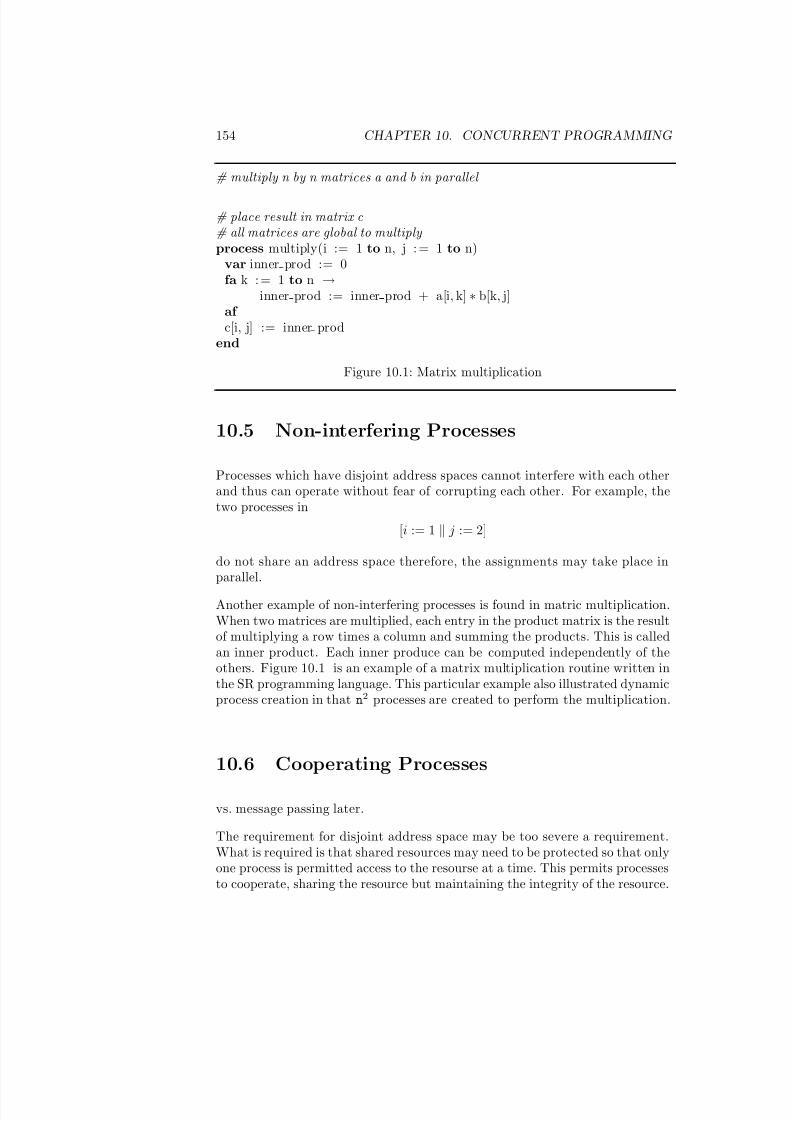
7/3/2019 Theory Introduction to Programming Languages
http://slidepdf.com/reader/full/theory-introduction-to-programming-languages-5584618bb4249 168/233
154 CHAPTER 10. CONCURRENT PROGRAMMING
# multiply n by n matrices a and b in parallel
# place result in matrix c# all matrices are global to multiply process multiply(i := 1 to n, j : = 1 to n)
var inner prod := 0fa k : = 1 to n →
inner prod := inner prod + a[i, k] ∗ b[k, j]af c[i, j] := inner prod
end
Figure 10.1: Matrix multiplication
10.5 Non-interfering Processes
Processes which have disjoint address spaces cannot interfere with each otherand thus can operate without fear of corrupting each other. For example, thetwo processes in
[i := 1 j := 2]
do not share an address space therefore, the assignments may take place inparallel.
Another example of non-interfering processes is found in matric multiplication.When two matrices are multiplied, each entry in the product matrix is the resultof multiplying a row times a column and summing the products. This is calledan inner product. Each inner produce can be computed independently of theothers. Figure 10.1 is an example of a matrix multiplication routine written inthe SR programming language. This particular example also illustrated dynamicprocess creation in that n2 processes are created to perform the multiplication.
10.6 Cooperating Processes
vs. message passing later.
The requirement for disjoint address space may be too severe a requirement.What is required is that shared resources may need to be protected so that onlyone process is permitted access to the resourse at a time. This permits processesto cooperate, sharing the resource but maintaining the integrity of the resource.
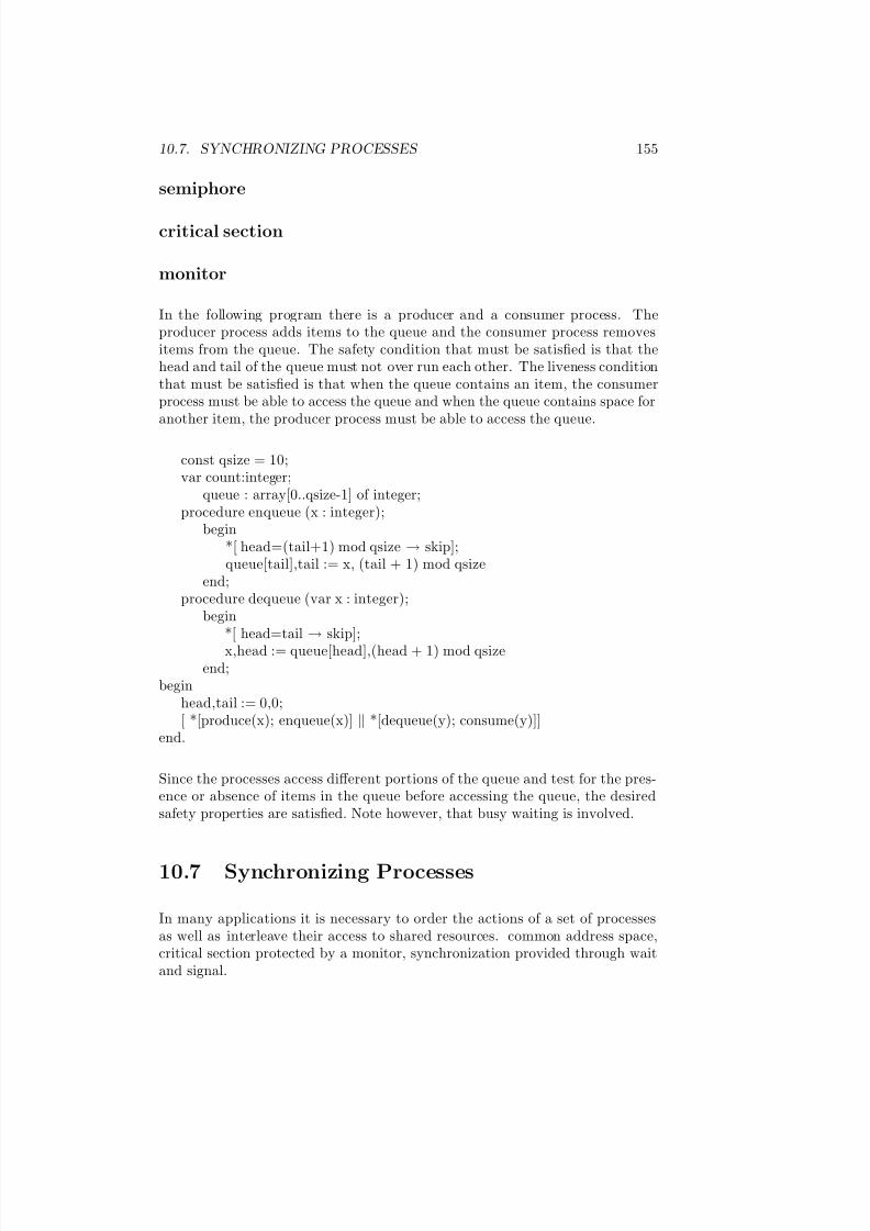
7/3/2019 Theory Introduction to Programming Languages
http://slidepdf.com/reader/full/theory-introduction-to-programming-languages-5584618bb4249 169/233
10.7. SYNCHRONIZING PROCESSES 155
semiphore
critical section
monitor
In the following program there is a producer and a consumer process. Theproducer process adds items to the queue and the consumer process removesitems from the queue. The safety condition that must be satisfied is that thehead and tail of the queue must not over run each other. The liveness conditionthat must be satisfied is that when the queue contains an item, the consumerprocess must be able to access the queue and when the queue contains space foranother item, the producer process must be able to access the queue.
const qsize = 10;var count:integer;
queue : array[0..qsize-1] of integer;procedure enqueue (x : integer);
begin*[ head=(tail+1) mod qsize → skip];queue[tail],tail := x, (tail + 1) mod qsize
end;procedure dequeue (var x : integer);
begin*[ head=tail → skip];
x,head := queue[head],(head + 1) mod qsizeend;
beginhead,tail := 0,0;[ *[produce(x); enqueue(x)] *[dequeue(y); consume(y)]]
end.
Since the processes access different portions of the queue and test for the pres-ence or absence of items in the queue before accessing the queue, the desiredsafety properties are satisfied. Note however, that busy waiting is involved.
10.7 Synchronizing Processes
In many applications it is necessary to order the actions of a set of processesas well as interleave their access to shared resources. common address space,critical section protected by a monitor, synchronization provided through waitand signal.
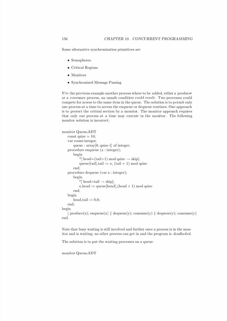
7/3/2019 Theory Introduction to Programming Languages
http://slidepdf.com/reader/full/theory-introduction-to-programming-languages-5584618bb4249 170/233
156 CHAPTER 10. CONCURRENT PROGRAMMING
Some alternative synchronization primitives are
• Semaphores
• Critical Regions
• Monitors
• Synchronized Message Passing
If in the previous example another process where to be added, either a produceror a consumer process, an unsafe condition could result. Two processes couldcompete for access to the same item in the queue. The solution is to permit onlyone process at a time to access the enqueue or dequeue routines. One approach
is to protect the critical section by a monitor. The monitor approach requiresthat only one process at a time may execute in the monitor. The followingmonitor solution is incorrect.
monitor Queue ADTconst qsize = 10;var count:integer;
queue : array[0..qsize-1] of integer;procedure enqueue (x : integer);
begin*[ head=(tail+1) mod qsize → skip];queue[tail],tail := x, (tail + 1) mod qsize
end;procedure dequeue (var x : integer);
begin*[ head=tail → skip];x,head := queue[head],(head + 1) mod qsize
end;begin
head,tail := 0,0;end;
begin[ produce(x); enqueue(x) dequeue(y); consume(y) dequeue(y); consume(y)]
end.
Note that busy waiting is still involved and further once a process is in the mon-itor and is waiting, no other process can get in and the program is deadlocked .
The solution is to put the waiting processes on a queue.
monitor Queue ADT

7/3/2019 Theory Introduction to Programming Languages
http://slidepdf.com/reader/full/theory-introduction-to-programming-languages-5584618bb4249 171/233
10.8. COMMUNICATING PROCESSES 157
const qsize = 10;var head, tail : integer;
queue : array[0..qsize-1] of integer;notempty, notfull : condition;
procedure enqueue (x : integer);begin
[ head=(tail+1) mod qsize → wait(notfull)2 head=(tail+1) mod qsize → skip];queue[tail],tail := x, (tail + 1) mod qsizesignal(notempty)
end;procedure dequeue (var x : integer);
begin[ head=tail → wait(notempty)
2 head=tail → skip];x,head := queue[head],(head + 1) mod qsize;signal(notfull)
end;begin
head,tail := 0,0;end;
begin[ produce(x); enqueue(x) dequeue(y); consume(y) dequeue(y); consume(y)]
end.
Busy waiting is no longer involved.
Livelock may result if there are more than one waiting process and when thesignal is received access is not granted fairly.
Starvation: (livelock) multiple processes waiting for access but access is notprovided in a fair manner
Coroutines.
Real-time Programming language issues
10.8 Communicating Processes
In the previous solution, it was assumed that the processes shared the addressspace and that synchronization was achieved by the use of monitor and con-dition queues. If the address spaces are disjoint, then both communicationand synchronization must be achieved through message passing. There are twochoices, message passing can be synchronous or asynchronous. When message
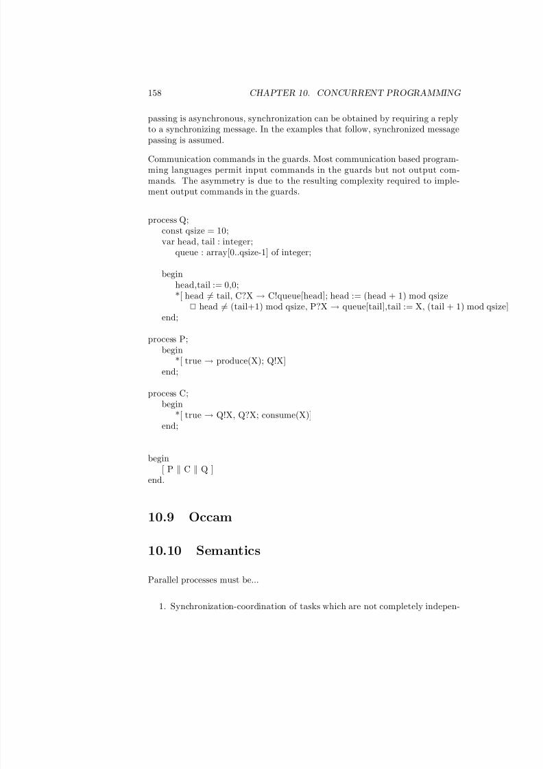
7/3/2019 Theory Introduction to Programming Languages
http://slidepdf.com/reader/full/theory-introduction-to-programming-languages-5584618bb4249 172/233
158 CHAPTER 10. CONCURRENT PROGRAMMING
passing is asynchronous, synchronization can be obtained by requiring a replyto a synchronizing message. In the examples that follow, synchronized messagepassing is assumed.
Communication commands in the guards. Most communication based program-ming languages permit input commands in the guards but not output com-mands. The asymmetry is due to the resulting complexity required to imple-ment output commands in the guards.
process Q;const qsize = 10;var head, tail : integer;
queue : array[0..qsize-1] of integer;
beginhead,tail := 0,0;*[ head = tail, C?X → C!queue[head]; head := (head + 1) mod qsize
2 head = (tail+1) mod qsize, P?X → queue[tail],tail := X, (tail + 1) mod qsize]end;
process P;begin
*[ true → produce(X); Q!X]end;
process C;
begin*[ true → Q!X, Q?X; consume(X)]
end;
begin[ P C Q ]
end.
10.9 Occam
10.10 Semantics
Parallel processes must be...
1. Synchronization-coordination of tasks which are not completely indepen-
7/3/2019 Theory Introduction to Programming Languages
http://slidepdf.com/reader/full/theory-introduction-to-programming-languages-5584618bb4249 173/233
10.11. RELATED ISSUES 159
dent.
2. Communication-exchange of information
3. Scheduling-priority,
4. Nondeterminism-arbitrary selection of execution path
Explicit Parallelism (message passing, semaphores, monitors)
Languages which have been designed for concurrent execution include Concur-rent Pascal, Ada and Occam. Application areas are typically operating systemsand distributed processing.
Ensemble activity
10.11 Related issues
Lazy evaluation vs Parallel execution
Backtracking vs Parallel execution
10.12 Examples
Pipelines
unix, pipeline sort, sieve
Systolic arrays
Dining Philosophers
10.13 Further Reading
Exercises
1. independent
2. pipe line

7/3/2019 Theory Introduction to Programming Languages
http://slidepdf.com/reader/full/theory-introduction-to-programming-languages-5584618bb4249 174/233
160 CHAPTER 10. CONCURRENT PROGRAMMING
3. synchronized
7/3/2019 Theory Introduction to Programming Languages
http://slidepdf.com/reader/full/theory-introduction-to-programming-languages-5584618bb4249 175/233
Chapter 11
PCN
11.1 Tutorial
Program Composition
Concurrent Programming Concepts
Getting Started
Example Program - compiling, linking, running
11.2 The PCN Language
PCN Syntax
Sequential Composition and Mutable Variables
Parallel Composition and Definitional Variables
Choice Composition
Definitional Variables as Communication Channels
Lists and Tuples
Stream Communication
Advanced Stream Handling
161
7/3/2019 Theory Introduction to Programming Languages
http://slidepdf.com/reader/full/theory-introduction-to-programming-languages-5584618bb4249 176/233
162 CHAPTER 11. PCN
11.3 Examples
Exercises

7/3/2019 Theory Introduction to Programming Languages
http://slidepdf.com/reader/full/theory-introduction-to-programming-languages-5584618bb4249 177/233
Chapter 12
Abstraction and
Generalization II
Encapsulate—To completely enclose.
Keywords and phrases: Modularity, encapsulation, function, procedure,abstract type, generic, library, object, class, inheritance, partition, package,
unit, separate compilation, linking, import, export, instance, scope.
• Partitions
• Separate compilation
– Linking
– Name and Type consistency
• Scope rules– Import
– Export
• Modules–collection of objects–definitions
• Package
163

7/3/2019 Theory Introduction to Programming Languages
http://slidepdf.com/reader/full/theory-introduction-to-programming-languages-5584618bb4249 178/233
164 CHAPTER 12. ABSTRACTION AND GENERALIZATION II
12.1 Encapsulation
The object part of a definition often contains other definitions which are saidto be local definitions. Such local definitions are not visible or available to bereferenced by other definitions. Thus the object part of a definition involves“information hiding”. This hidden information is sometimes made available byexporting the names.
The work of constructing large programs is divided among several people, eachof whom must produce a part of the whole. Each part is called a module andeach programmer must be able to construct his/her module without knowingthe internal details of the other parts. This is only possible when each moduleis is separated into an interface part and an implementation part. Theinterface part describes all the information required to use the module whilethe implementation part describes the implementation. This idea is alreadypresent in most programming languages in the manner in which functions andprocedures are defined. Function and procedure definitions usually areseparated into two parts. The first part gives the subprogram’s name andparameter requirements and the second part describes the implementation. Amodule is a generalization of the concept of abstraction in that a module ispermitted to contain a collection of definitions. An additional goal of modulesis to confine changes to a few modules rather than throughout the program.
While the concept of modules is a useful abstraction, the full advantages of modules are gained only when modules may be written, compiled and possiblyexecuted separately. In many cases modules should be able to be tested
independently of other modules.
In this section we consider various language design considerations which canbe used as weapons in the war against complexity, the pragmatics of programming. In particular, we discuss scope, modularity.
Advantages
• reduction in complexity
• team programming
• maintainability
• reusability of code
• project management
Implementation
• common storage area – Fortran

7/3/2019 Theory Introduction to Programming Languages
http://slidepdf.com/reader/full/theory-introduction-to-programming-languages-5584618bb4249 179/233
12.2. ADTS 165
• include directive – C++
• subroutine library
Typical applications:
• subroutine packages – mathematical, statistical etc
• ADTs
examples from Ada, C++, etc
12.2 ADTs
An even more effective approach is to separate the signatures of the operationsfrom the bodies of the operations and the type representation so that theoperation bodies and type representation can be compiled separately. Thisfacilitates the development of software in that when an abstract data type’srepresentation is changed (e.g. to improve performance) the changes arelocalized to the abstract data type.
name : adt
operation signatures
...
name : adt body
type representation definition
operation bodies
...
12.3 Partitions
Definition 12.1 A partition of a set is a collection of disjoint sets whose
union is the set.
There are a number of mechanisms for partitioning program text. Functionsand procedures are among the most common. However, the result is still asingle file. When the partitions of program text are arranged in separate files,the partitions are called modules. Here are several program partitioningmechanisms.
7/3/2019 Theory Introduction to Programming Languages
http://slidepdf.com/reader/full/theory-introduction-to-programming-languages-5584618bb4249 180/233
166 CHAPTER 12. ABSTRACTION AND GENERALIZATION II
• Separate declaration of data and code
• Procedures
• Functions
• ADTs
• Modules
Partitioning of program text is desirable to provide for separate compilationand for pipeline processing of data.
There are a number of mechanisms for combining the partitions into a singleprogram for the purposes of compilation and execution. The include
statement is provided in a number of languages. It is a compiler directive withdirects the compiler to textually include the named file in the source program.In some systems the partitions may be separately compiled and there is alinking phase in which the compiled program modules are linked together forexecution. In other systems, at run-time any missing function or procedureresults in a run-time search for the missing module which if found is thenexecuted or if not found results in a run-time error.
12.4 Scope Rules
The act of partitioning a program raises the issue of the scope of names.Which objects with in the module are to be visible outside the module? Theusual solution is to designate some names to be exported and others to beprivate or local to the module and invisible to other modules. In case theremight be name conflict between exported names from modules, modules areoften permitted to designate names that are to be imported from designatedmodules or to qualify the name with the module name.
The scope rules for modules define relationships among the names within themodules. There are four choices.
• All local names visible globally.
• All external names visible locally.
• Only local explicitly exported names visible globally.
• Only external names explicitly imported are visible locally.
Name conflict is resolved via qualification with the module name.
7/3/2019 Theory Introduction to Programming Languages
http://slidepdf.com/reader/full/theory-introduction-to-programming-languages-5584618bb4249 181/233
12.5. MODULES 167
12.5 Modules
A module is a named program unit which is an (more or less) independententity. In program construction the module designer must answer thefollowing questions.
• What is the module’s purpose?
• How does it achieve that purpose?
Programming in the large is concerned with programs that are notcomprehensible by a single individual and are developed by teams of programmers. At this level programs must consist of modules that can be
written, compiled, and tested independently of other modules. A module has asingle purpose, and has a narrow interface to other modules. It is likely to bereuseable (able to be incorporated into may programs) and modifiable without forcing changes in other modules.
Modules must provide answers to two questions:
• What is the purpose of the module?
• How does it achieve that purpose?
The what is of concern to the user of the module while the how is of concern tothe implementer of the module.
Functions and procedures are simple modules. Their signature is a descriptionof what they do while their body describes how it is achieved. More typically amodule encapsulates a group of components such as types, constants,variables, procedures, functions and so on.
To present a narrow interface to other modules, a module makes only a fewcomponents visible outside. Such components are said to be exported by themodule. The other components are said to be hidden inside the module. Thehidden components are used to implement the exported components.
Access to the components is often by a qualified name – module name.component name. When strong safety considerations are important, modules
using components of another module may be required to explicitly import therequired module and the desired components.
Exercises
1. Algebraic Semantics: stack, tree, queue, grade book etc

7/3/2019 Theory Introduction to Programming Languages
http://slidepdf.com/reader/full/theory-introduction-to-programming-languages-5584618bb4249 182/233
168 CHAPTER 12. ABSTRACTION AND GENERALIZATION II
2. Lexical Scope Rules
3. Dynamic Scope Rules
4. Parameter Passing
5. Run-time Stack

7/3/2019 Theory Introduction to Programming Languages
http://slidepdf.com/reader/full/theory-introduction-to-programming-languages-5584618bb4249 183/233
Chapter 13
Object-Oriented
Programming
Object-oriented programming is characterized by programming with objects,messages, and hierarchies of objects.
Keywords and phrases: Abstract Data Type, object-based, object-oriented,
Inheritance, Object, sub-type, super-type, sub-range, sub-class, super-class,polymorphism, overloading, dynamic type checking, Class, Instance, method,message
• History
– Simula
– ADT
– Small-Talk– Modula-2, C++, Eiffel
• Subtypes (subranges)
• Generic types
• Inheritance – Scope generalization
169
7/3/2019 Theory Introduction to Programming Languages
http://slidepdf.com/reader/full/theory-introduction-to-programming-languages-5584618bb4249 184/233
170 CHAPTER 13. OBJECT-ORIENTED PROGRAMMING
• OOP
– Objects–state + operations– Object Classes– Class, Subclass
• Objects–state + operations
• Object Classes– Class, Subclass
• Inheritance mechanism
Object-oriented programming shifts the emphasis from data as passiveelements acted on by procedures to data as active elements interacting withtheir environment. From control flow to interacting objects.
Object-oriented programming developed out of simulation programs. Theconceptual model used is that the structure of the simulation should reflectthe environement that is being simulated. For example, if an industrial processis to be simulated, then there should be an object for each entity involved inthe process. The objects interact by sending messages.
Each object is designed around a data invariant.
is an abstraction and generalization of imperative programming. Imperativeprogramming involves a state and a set of operations to transform the state.Object-oriented programming involves collections of objects each with a stateand a set of operations to transform the state. Thus, object-oriented
programming focuses on data rather than on control. As in the real world,objects interact so object-oriented programming uses the metaphor of messagepassing to capture the interaction of objects.
Functional objects are like values, imperative objects are like variables, activeobjects are like processes.
Aternatively, OOP, an object is a parameter (function and logic), an object isa mutable self (imperative).
Programming in an imperative programming language requires theprogrammer to think in terms of data structures and algorithms formanipulating the data structure. That is, data is placed in a data structure
and the data structure is manipulated by various procedures.
Programming in an object-oriented language requires the programmer to thinkin terms of a hierarchy of objects and the properties possessed by the objects.The emphasis is on generality and reusability.
Procedures and functions are the focus of programming in an imperativelanguage. Object-oriented programming focuses on data, the objects and the

7/3/2019 Theory Introduction to Programming Languages
http://slidepdf.com/reader/full/theory-introduction-to-programming-languages-5584618bb4249 185/233
171
operations required to satisfy a particular task.
Object-oriented programming, as typified by the Small-talk model, views theprogramming task as dealing with objects which interact by sending messagesto each other. Concurrency is not necessarily implied by this model anddestructive assignment is provided. In particular, to the notion of an abstractdata type, OOP adds the notion of inheritance, a hierarchy of relationshipsamong types. The idea of data is generalized from simple items in a domain todata type (a domain and associated operations) to an abstract data type (theaddition of information hiding) to OOP & inheritance.
Here are some definitions to enable us to speak the language of object-orientedprogramming.
Definition 13.1
Object: Collection of private data and public operations.
Class: Description of a set of objects. (encapsulated type: partitioned intoprivate and public)
Instance: An instance of a class is an object of that class.
Method: A procedure body implementing an operation.
Message: A procedure call. Request to execute a method.
Inheritance: Extension of previously defined class. Single inheritance,multiple inheritance
Subtype principle: a subtype can appear wherever an object of a supertype isexpected.
I think a classification which helps is to classify languages as object-based andobject-oriented. A report we recently prepared on OO technology trendsreported that object-based languages support to varying degrees: object-basedmodularity, data abstraction (ADTs) encapsulation and garbage collection.Object-oriented languages additionally include to varying degrees: groupingobjects into classes, relating those classes by inheritance, polymorphism and
dynamic binding, and genericity.
Dr. Bertrand Meyer in his book ’Object-oriented Software Construction’(Prentice Hall) gives his ’seven steps to object-based (oriented) happiness’
1) Object-based modular structure 2) Data abstraction 3) Automatic memorymanagement 4) Classes 5) Inheritance 6) Polymorphism and Dynamic Binding7) Multiple and Repeated Inheritance
7/3/2019 Theory Introduction to Programming Languages
http://slidepdf.com/reader/full/theory-introduction-to-programming-languages-5584618bb4249 186/233
172 CHAPTER 13. OBJECT-ORIENTED PROGRAMMING
13.1 History
• Simula
• Small-Talk
• Modula-2, C++, Eiffel
• Flavors, CLOS
13.2 Subtypes (subranges)
The subtype principle states that a subtype may appear wherever an element
of the super type is expected.
13.3 Objects
Objects are collections of operations that share a state. The operationsdetermine the messages (calls) to which the object can respond, while theshared state is hidden from the outside world and is accessible only to theobject’s operations. Variables representing the internal state of an object arecalled instance variables and its operations are called methods. Its collection of methods determines its interface and its behavior .
Objects which are collections of functions but which do not have a state arefunctional objects. Functional objects are like values, they have the ob ject-likeinterface but no identity that persists between changes of state. Functionalobjects arise in logic and functional programming languages.
Syntactically, a functional object can be represented as:
name : object
methods
...
For example,
Objects which have an updateable state are imperative objects. Imperativeobjects are like variables. They are the objects of Simula, Smalltalk and C++.They have a name, a collection of methods which are activated by the receiptof messages from other objects, and instance variables which are shared by themethods of the object but inaccessible to other objects.
7/3/2019 Theory Introduction to Programming Languages
http://slidepdf.com/reader/full/theory-introduction-to-programming-languages-5584618bb4249 187/233
13.4. CLASSES 173
Syntactically, an imperative object can be represented as:
name : object
variables
...
methods
...
Objects which may be active when a message arrives are active objects. Incontrast, functional and imperative objects are passive unless activated by amessage. Active objects have three modes: when there is nothing to do the
object is dormant , when the agent is executing it is active, and when an objectis waiting for a resource or the completion of subtasks it is waiting . Messagessent to an active object may have to wait in queue until the object finishes atask. Message passing among objects may be synchronous or asynchronous.
13.4 Classes
Classes serve as templates from which objects can be created. Classes have thesame instance variables and operations as corresponding objects but theirinterpretation is different. Instance variables in an object represent actual variables while class instance variables are potential , being instantiated onlywhen an object is created.
We may think of a class as specifying a behavior common to all objects of theclass. The instance variables specify a structure (data structure) for realizingthe behavior. The public operations of a class determine its behavior while theprivate instance variables determine its structure.
Private copies of a class can be created by a make-instance operation, whichcreates a copy of the class instance variables that may be acted on by the classoperations.
Syntactically, a class can be represented as:
name : class
instance variables
...
class variables
...
7/3/2019 Theory Introduction to Programming Languages
http://slidepdf.com/reader/full/theory-introduction-to-programming-languages-5584618bb4249 188/233
174 CHAPTER 13. OBJECT-ORIENTED PROGRAMMING
instance methods
...
class methods
...
Classes specify the behavior common to all elements of the class. Theoperations of a class determine the behavior while the instance variablesdetermine the structure.
Algebraic semantics
Many sorted algebras may be used to model classes.
13.5 Inheritance
Inheritance allows us to reuse the behavior of a class in the definition of newclasses. Subclasses of a class inherit the operations of their parent class andmay add new operations and new instance variables.
Inheritance captures a form of abstraction called super-abstraction , that
complements data abstraction. Inheritance can express relations amongbehaviors such as classification, specialization, generalization, approximation,and evolution.
Inheritance classifies classes in much the way classes classify values. Theability to classify classes provides greater classification power and conceptualmodeling power. Classification of classes may be referred to as second-orderclassification. Inheritance provides second-order sharing, management, andmanipulation of behavior that complements first-order management of objectsby classes.
Syntactically, inheritance may be specified in a class as:
name : class
super class
...
instance variables
{ as before }
7/3/2019 Theory Introduction to Programming Languages
http://slidepdf.com/reader/full/theory-introduction-to-programming-languages-5584618bb4249 189/233
13.6. TYPES AND CLASSES 175
What should be inherited? Should it be behavior or code: specification orimplementation? Behavior and code hierarchies are rarely compatible witheach other and are often negatively correlated because shared behavior andshared code have different requirements.
Representation, Behavior, Code
DYNAMIC/STATIC/INHERITANCE
Inheritance and OOP
Type hierarchy
Semantics of inheritance in the functional paradigm.
type op params = case op of
f0 : f0 params
...
fn : fn params
otherwise : supertype op params
where
f0 params = def0
...
fn params = defn
inheritance in the logic programming paradigm.
object(structure,methodslist).
isa(type1,type2).
object(rectangle(Length,Width),[area(A is Length*Width)]).
Algebraic semantics
Order-sorted algebras are required to capture the ordering relations amongsorts that arise in subtypes and inheritance.
13.6 Types and Classes
The concept of a type and the concept of a class have much in common anddepending on the point of view, they may be indistinguishable. Thedistinction between types and classes may be seen when we examine the

7/3/2019 Theory Introduction to Programming Languages
http://slidepdf.com/reader/full/theory-introduction-to-programming-languages-5584618bb4249 190/233
176 CHAPTER 13. OBJECT-ORIENTED PROGRAMMING
compare the inheritance relationship between types and subtypes with theinheritance relationship between classes and subclasses.
Example 13.1 The natural numbers are a subtype of the integers but whilesubtraction is defined for all pairs of integers it is not defined for all pairs of natural numbers.
This is an example of subtype inheritance. Subtypes are defined by additionalconstraints imposed on a type. The set of values satisfying a subtype is asubset of the set of values satisfying the type and subtypes inherit a subset of the behaviors of the type.
Example 13.2 The integers are a subclass of the natural numbers since, the
subtraction operation of the natural numbers can be extended to subtraction for integers.
Example 13.3 The rational numbers are a subclass of the integers since, they can be defined as pairs of natural numbers and the arithmetic operations on therational numbers can be defined in terms of the arithmetic operations on natural numbers.
These are examples of subclass inheritance. Subclasses are defined byextending the class behavior. This means that subclasses are more looselyrelated to their parent than a subtype to a type. Both state and methods maybe extended.
Subtyping strongly contrains behavior while subclassing is an unconstrainedmechanism. It is the inheritance mechanism of OOP that distingushesbetween types and classes.
These examples illustrate that subtype inheritance is different from subclassinheritance. Subclasses may define behavior completely unrelated to theparent class.
Types are used for type checking while classes are used for generating andmanaging objects with uniform properties and behaviors. Every class is atype. However, not every type is a class, since predicates do not necessarylydetermine object templates. We will use the term type to refer to structure
and values while the term class will be used to refer to behavior.
13.7 Examples
Queue – insert rear, delete front
7/3/2019 Theory Introduction to Programming Languages
http://slidepdf.com/reader/full/theory-introduction-to-programming-languages-5584618bb4249 191/233
13.8. FURTHER READING 177
Deque – insert front, delete front, insert rear, delete rear
Stack – push, pop
List – cons, head, tail
Binary tree – insert, remove, traverse
Doublely linked list –
Graph – linkto, path,
Natural numbers – Ds
Integers – (=-,Ds)
Rationals
Reals – (+-,Ds,Ds)
Complex (a,b) or (r,θ)
13.8 Further Reading
Much of this section follows Peter Wegner[31].
13.9 Exercises
• Stack
• Queue
• Tree
• Construct a “turtle graphics”
• Construct a table handler
• Grammar
• Prime number sieve
• Account, Checking, Savings
• Point, circle

7/3/2019 Theory Introduction to Programming Languages
http://slidepdf.com/reader/full/theory-introduction-to-programming-languages-5584618bb4249 192/233
178 CHAPTER 13. OBJECT-ORIENTED PROGRAMMING
7/3/2019 Theory Introduction to Programming Languages
http://slidepdf.com/reader/full/theory-introduction-to-programming-languages-5584618bb4249 193/233
Chapter 14
Pragmatics
14.1 Syntax
In view of abstract syntax it may seem that concrete syntax does not matter.In fact, details such as placement of keywords, semicolons and case do matter.
In Pascal the semicolon is a statement separator. In C the semicolon is astatement terminator. Pascal permits the empty statement. This may lead tounintended results. A misplaced semicolon can change the meaning of aprogram.
Algol-68 and Modula-2 require closing keywords. Modula-2 uses end whileAlgol-68 uses the reverse of the opening keyword for example,
if < conditionalexpression > then < command > fi
The assignment operator varies among imperative programming languages. InPascal and Ada it is := while in FORTRAN and C it is = and in APL it is ←.The choice in FORTRAN and C is unfortunate since assignment is differentfrom equality. This leads to the use of == for equality in C and .EQ. inFORTRAN.
14.2 Semantics
The use of formal semantic description techniques is playing an increasing rolein software engineering.
179
7/3/2019 Theory Introduction to Programming Languages
http://slidepdf.com/reader/full/theory-introduction-to-programming-languages-5584618bb4249 194/233
180 CHAPTER 14. PRAGMATICS
Algebraic semantics are useful for the specification of abstract data types.
For effective use axiomatic semantics require support for program varification.
Denotational semantics are beginning to play a role in compiler constructionand a prescriptive rather than a descriptive role in the design of programminglanguages.
Operational semantics –
14.3 Bindings and Binding Times
Bindings may occur at various times from the point of language definitionthrough program execution. The time at which the binding occurs is termedthe binding time.
Four distinct binding times may be distinguished.
1. Language design time. Much of the structure of a programming languageis fixed and language design time. Data types, data structures, commandand expression forms, and program structure are examples of languagefeatures that are fixed at language design time. Most programminglanguages make provision for extending the language by providing forprogrammer defined data types, expressions and commands.
2. Language implementation time. Some language features are determinedby the implementation. Programs that run on one computer may not runor give incorrect results when run on another machine. This occurs whenthe hardware differs in its representation of numbers and arithmetic. Forexample, the maxint of Pascal is determined by the implementation. TheC programming language provides access to the underlying machine andtherefore programs which depend on the characteristics of the underlyingmachine may not perform as expected when moved to another machine.
3. Program translation time. The binding between the source code and theobject code occurs at program translation time. Programmer definedvariables and types are another example of bindings that occur atprogram translation time.
4. Program execution time. Binding of values to variables and formalparameters to actual parameters occur during program execution.
Early binding often permits more efficient execution of programs while latebinding permits more flexibility. The implementation of recursion may requireallocation of memory at run-time in contrast a one time to allocation of memory at compile-time.
7/3/2019 Theory Introduction to Programming Languages
http://slidepdf.com/reader/full/theory-introduction-to-programming-languages-5584618bb4249 195/233
14.4. VALUES AND TYPES 181
14.4 Values and Types
The primitive types are implemented using both the underlying hardware andspecial purpose software. So that only appropriate operations are applied tovalues, the value’s type must be known. The type information is contained ina descriptor. When the type of a value is known at compile time the typedescriptor is a part of the symbol table and is not needed at run-time andtherefore, the descriptor is discarded after compilation. When the type a valueis not known until run-time, the type descriptor must be associated with thevalue to permit type checking.
Boolean values are implemented using a single bit of storage. Since singlebits are not usually addressable, the implementation is extended to be a single
addressable unit of memory. In this case either a single bit within theaddressable unit is used for the value or a zero value in the storage unitdesignates false while any non-zero value designates true.
Integer values are most often implemented using a hardware defined integerstorage representation. The integer arithmetic and relational operations areimplemented using the set of hardware operations. The storage unit is dividedinto a sign and a binary number. Since the integers form an infinite set, only asubrange of integers is provided. Some languages (for example Lisp andScheme) provide for a greatly extended range by implementing integers in listsand providing the integer operations in software. This provides for “infinite”precision arithmetic.
Natural number values are most often implemented using the hardwaredefined storage unit. The advantage of providing an natural number type isthat an additional bit of storage is available thus providing larger positivevalues than are provided for integer values.
Rational number values may be implemented as pairs of integers. Rationalsare provided when it is desired to avoid the problems of roundoff andtruncation which occurs when floating-point numbers are used to representrational numbers.
Real number values are most often implemented using a hardware definedfloating-point representation. The floating-point arithmetic and relationaloperations are implemented using the set of hardware operations. Some
floating-point operations such as exponentiation are provided in software. Thestorage unit is divided into a mantissa and an exponent. Sometimes more thanone storage unit is used to provide greater precision.
Character values are almost always supported by the underlying hardwareand operating system.
Enumeration values are usually represented by a subsequence of the integers
7/3/2019 Theory Introduction to Programming Languages
http://slidepdf.com/reader/full/theory-introduction-to-programming-languages-5584618bb4249 196/233
182 CHAPTER 14. PRAGMATICS
and as such inherit an appropriate subset of the integer operations.
Where strings are treated as a primitive type, they are usually of fixed lengthand their operations are implemented in hardware.
Abstract data types are best implemented with pointers. The user programholds a pointer to a value of the abstract type. This use of pointers is quitesafe since the pointer manipuation is restricted to the implementation moduleand the pointer is notationally hidden.
14.5 Computational Models
14.6 Procedures and Functions
In the discussion which follows, the term subprogram will be used to refer towhole programs, procedures and functions.
A program may be composed of a main program which during execution maycall subprograms which in turn may call other subprograms and so on. Whena subprogram is called, the calling subprogram waits for the called subprogramto terminate. Each subprogram is expected to eventually terminate and returncontrol to the calling subprogram. The execution of the calling subprogramresumes at the point immediately following the point of call. Each subprogrammay have its own local data which is found in an activation record . Anactivation record consists of an association between variables and the value towhich they are assigned. An activation record may be created each time asubprogram is called and destroyed when the subprogram terminates.
The run time environment must keep track of the current instruction and thereferencing environment for each active or waiting program so that when asubprogram terminates, the proper instruction and data environment may beselected for the calling subprogram.
The current instruction of the calling subprogram is maintained on a stack.When a subprogram is called, the address of the instruction following the callof the calling program is pushed on the stack. When a subprogram terminates,the instruction pointer is set to the address on the top of the stack and theaddress popped off the stack. The stack is often called the return address stack .
The addresses of the current environment is also maintained on a stack. Thetop of the stack always points to the current environment. When a subprogramis called, the address of the new environment is pushed on the stack. When asubprogram terminates, the stack is popped revealing the previousenvironment. The stack is often called the dynamic links because the stack

7/3/2019 Theory Introduction to Programming Languages
http://slidepdf.com/reader/full/theory-introduction-to-programming-languages-5584618bb4249 197/233
14.7. SCOPE AND BLOCKS 183
contains links (pointers) which reveal the dynamic history of the program.
When a programming language does not permit recursive procedures and datastructure size is independent of computed or input data, the maximum storagerequirements of the program can be determined at compile time. Thissimplifies the run time support required by the program and it is possible tostatically allocate the storage used during program execution.
14.7 Scope and Blocks
A variables declared within a block have a lifetime which extends from themoment an activation record is created for the block until the activation
record for the block is destroyed. A variable is bound to an offset within theactivation record at compile time. It is bound to a specific storage locationwhen the block is activated and becomes a part of storage.
Dynamic Scope Rules
Conceptually the dynamic scope rules may be implemented as follows. Eachvariable is assigned a stack to hold the current values of the variable.
When a subprogram is called, a new uninitialized stack element is pushed onthe stack corresponding to each variable in the block.
A reference to a variable involves the inspection or updating of the topelement of the appropriate stack. This provides access to the variable inclosest block with respect to the dynamic calling sequence.
When a subprogram terminates, the stacks corresponding to the variables of the block are popped, restoring the calling environment.
Static Scope Rules
The static scope rules are implemented as follows. The data section of each
procedure is associated with an activation record. The activation recordsare dynamically allocated space on a runtime stack. Each recursive call isassociated with it own activation record. Associated with each activationrecord is a dynamic link which points to the previous activation records, areturn address which is the address of the instruction to be executed uponreturn from the procedure and a static link which provides access to thereferencing environment.
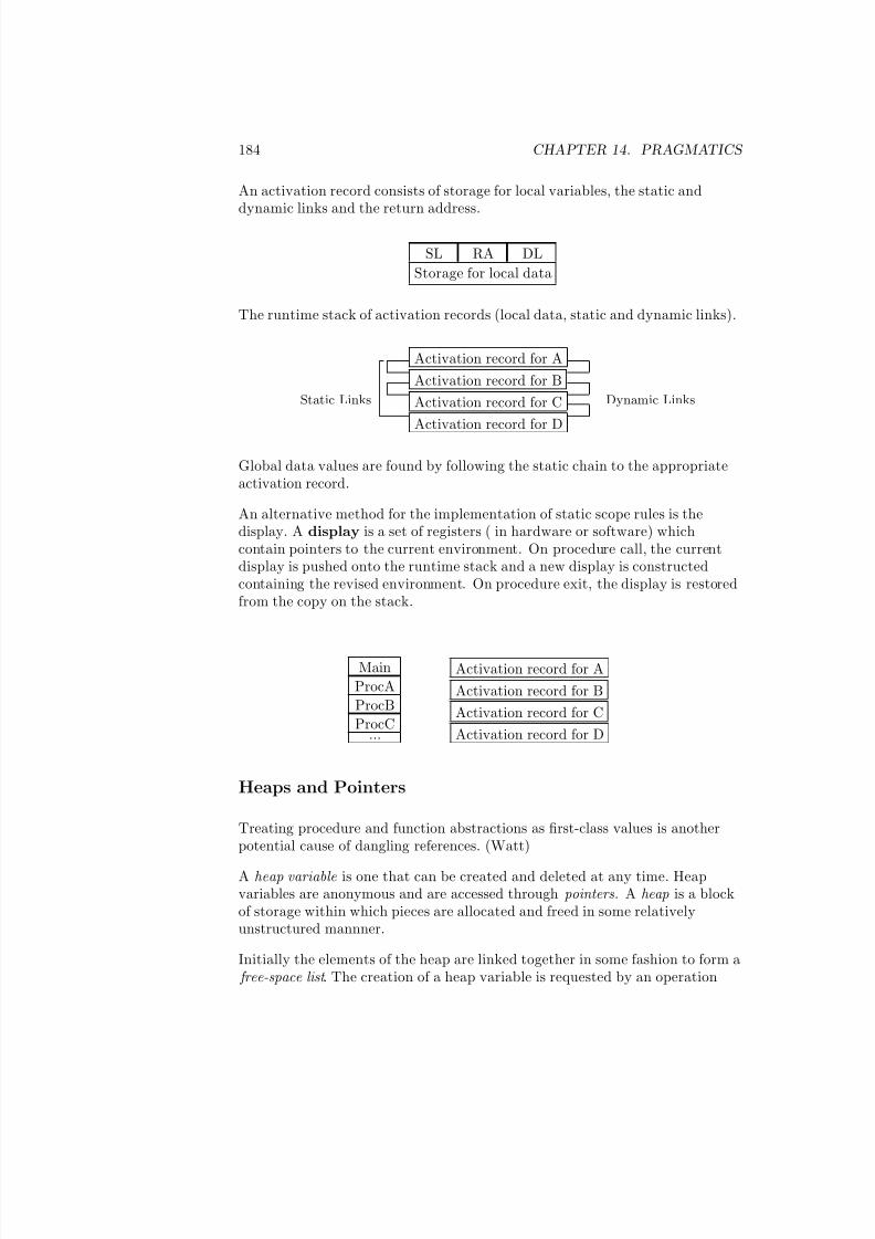
7/3/2019 Theory Introduction to Programming Languages
http://slidepdf.com/reader/full/theory-introduction-to-programming-languages-5584618bb4249 198/233
184 CHAPTER 14. PRAGMATICS
An activation record consists of storage for local variables, the static anddynamic links and the return address.
SL RA DL
Storage for local data
The runtime stack of activation records (local data, static and dynamic links).
Activation record for A
Activation record for B
Activation record for C
Activation record for D
Static Links Dynamic Links
Global data values are found by following the static chain to the appropriateactivation record.
An alternative method for the implementation of static scope rules is thedisplay. A display is a set of registers ( in hardware or software) whichcontain pointers to the current environment. On procedure call, the currentdisplay is pushed onto the runtime stack and a new display is constructedcontaining the revised environment. On procedure exit, the display is restoredfrom the copy on the stack.
Main
ProcA
ProcB
ProcC...
Activation record for A
Activation record for B
Activation record for C
Activation record for D
Heaps and Pointers
Treating procedure and function abstractions as first-class values is anotherpotential cause of dangling references. (Watt)
A heap variable is one that can be created and deleted at any time. Heapvariables are anonymous and are accessed through pointers. A heap is a blockof storage within which pieces are allocated and freed in some relativelyunstructured mannner.
Initially the elements of the heap are linked together in some fashion to form a free-space list . The creation of a heap variable is requested by an operation
7/3/2019 Theory Introduction to Programming Languages
http://slidepdf.com/reader/full/theory-introduction-to-programming-languages-5584618bb4249 199/233
14.7. SCOPE AND BLOCKS 185
called an allocator which returns a pointer to the newly created variable. Toallocate an element, the first element on the list is removed from the list and apointer to it is returned to the operation requesting the storage.
The heap variable’s lifetime extends from the time it is created until it is nolonger accessable.
Often there is an operation called a deallocator which forcibly deletes a givenheap variable. When an element is deallocated (freed), it is simply linked backin at the head of the free-space list. If all references to heap variable aredestroyed, the heap variable is inaccessable and becomes garbage. When avariable becomes garbage, its memory space is unusable by other variablessince a means of referencing it must exist in order to return the space to thefree-space list.
When deallocation is under the control of the programmer, it is a potentialsource of problems. If a programmer deallocates a variable, any remainingpointers to the deleted heap variable become dangling references.
Garbage and dangling references are potentially troublesome for theprogrammer. If garbage accumulates, available storage is gradually reduceduntil the program may be unable to continue for lack of known free space. If aprogram attempts to modify through a dangling reference a structure that hasbeen deallocated (destroyed), the contents of an element of free-space may bemodified. This may cause the remainder of the free-space to become garbageor a portion of the program to become linked to free-space. The deallocatedspace could be reallocated to some other structure resulting in similar
problems.The problem of dangling references can be eliminated.
One solution is to restrict assignment so that references to local variables maynot be assigned to variables with a longer lifetime. This restriction mayrequire runtime checks and sometimes restrict the programmer.
Another solution is to maintain reference counts with each heap variable. Aninteger called the reference count is associated with each heap element. Thereference count indicates the number of pointers to the element that exist.Initially the count is set to 1. Each time a pointer to the element is createdthe reference count is increased and each time a pointer to the element isdestroyed the reference count is decreased. Its space is not deallocated untilthe reference count reaches zero. The method of reference counting results insubstantial overhead in time and space.
Another solution is to provide garbage collection . The basic idea is to allowgarbage to be generated in order to avoid dangling references. When thefree-space list is exhausted and more storage is needed, computation is
7/3/2019 Theory Introduction to Programming Languages
http://slidepdf.com/reader/full/theory-introduction-to-programming-languages-5584618bb4249 200/233
186 CHAPTER 14. PRAGMATICS
suspended and a special procedure called a garbage collector is started whichidentifies garbage and returns it to the free-space list.
There are two stages to garbage collection a marking phase and a collecting phase.
Marking phase: The marking phase begins outside the heap with thepointers that point to active heap elements. The chains of pointers arefollowed and each heap element in the chain is marked to indicate that itis active. When this phase is finished only active heap elements aremarked as active.
Collecting phase: Ub the collecting phase the heap is scanned and each
element which is not active is returned to the free-space list. During thisphase the marked bits are reset to prepare for a later garbage collection.
This unuseable space may be reclamed by a garbage collector . A heap variableis alive as long as any reference to it exists.
Coroutines
Coroutines are used in discrete simulation languages and, for some problems,provide a control structure that is more natural than the usual hierarchy of subprogram calls.
Coroutines may be thought of as subprograms which are not required toterminate before returning to the calling routine. At a later point the callingprogram may “resume” execution of the coroutine at the point from whichexecution was suspended. Coroutines then appear as equals with controlpassing from one to the other as necessary. From two coroutines it is naturalto extend this to a set of coroutines.
From the description given of coroutines, it is apparent that coroutines shouldnot be recursive. This permits us to use just one activation record for eachcoroutine and the address of each activation record can be staticallymaintained.
Each activation record is extended to include a location to store the CI for thecorresponding coroutine. It is initialized with the location of the firstinstruction of the coroutine. When coroutine encounters a resume operation, itstores the address of its next instruction in it own activation record. Theaddress of the CI for the resumed coroutine is obtained from the activationrecord of the resumed coroutine.
7/3/2019 Theory Introduction to Programming Languages
http://slidepdf.com/reader/full/theory-introduction-to-programming-languages-5584618bb4249 201/233
14.8. PARAMETERS AND ARGUMENTS 187
Concurrency
14.8 Parameters and Arguments
In the previous sections, the arguments to an invocation are textuallysubstituted for the parameters. That is, the body of the abstract is rewrittenwith the arguments substituted for the parameters.
Eager vs Lazy evaluation
An abstraction is said to be strict in a parameter if it is sure to need the value
of the parameter and non-strict in a parameter it is not sure to require thevalue of the parameter. The arithmetic operators are strict but the conditionalexpression is not strict in its second and third arguments since the selection of the second or third argument is dependent on the value of the first argument.
The programming language Scheme assumes that all functions are strict intheir parameters, therefore, the parameters are evaluated when the function iscalled. This evaluation scheme is called eager evaluation . This is not alwaysdesirable and so Scheme provides for the quote operator to inform a functionnot to evaluate its parameters. Miranda evaluates the arguments only whenthe value is required. This evaluation scheme is called normal-order evaluation or lazy evaluation .
Argument Passing Mechanisms
With respect to functional and logic programming languages, the question of how to pass parameters is relatively simple. The imperative programmingparadigm is another issue.
Copy Mechanisms
The copy mechanism requires values to be copied into an abstraction when itis entered and copied out of the abstraction when the abstraction is exited.The formal parameters are local variables. Therefore, the actual parameter iscopied into the local variable on entry to the abstraction and copied out of thelocal variable to the actual parameter on exit from the abstraction.
The parameters of C++, the value parameter of Modula-2 and the in parameter of Ada are examples of parameters which may be passed by usingthe copy mechanism. The value of the actual parameter is copied into the
7/3/2019 Theory Introduction to Programming Languages
http://slidepdf.com/reader/full/theory-introduction-to-programming-languages-5584618bb4249 202/233
188 CHAPTER 14. PRAGMATICS
formal parameter on entry but the value of the formal parameter is not copiedto the actual parameter on exit. In imperative languages, copying isunnecessary if the language prohibits assignment to the formal parameter. Insuch a case, the parameter may be passed by reference. This form of parameter passing is often referred to as passing by value
Ada’s out parameter , and function results in general are examples of parameters which may be passed by using the copy mechanism. The value of the actual parameter is not copied into the formal parameter on entry but thevalue of the formal parameter is copied into the actual parameter upon exit.In Pascal the function name is used as the formal parameter and assignmentsmay be made to the function name. This form of parameter passing is oftenreferred to as passing by result.
When the passing by value and result are combined, the passing mechanism isreferred to as passing by value-result. Ada’s in out parameter is anexample of a parameter which may be passed by this form of the copymechanism. The value of the actual parameter is copied into the formalparameter on entry and the value of the formal parameter is copied into theactual parameter upon exit.
The copy mechanism has some disadvantages. The copying of large compositevalues (arrays etc) is expensive and the parameters must be assignable (eg filetypes in Pascal are not assignable).
Definitional Mechanisms
The effect is as if the abstraction body were surrounded by a block, in whichthere is a definition that binds the formal parameter to the actual parameter.
The reference parameter of Modula-2, the array and structure parameters of C++ are passed using this mechanism.
Name
Algol-60 provides a parameter passing mechanism which is based on that of the functional model however it does not provide the generality that is
required in the imperative model as the following example shows.
Algol-60, Jensen’s device
procedure swap(x,y:sometype);
var x:sometype
begin
7/3/2019 Theory Introduction to Programming Languages
http://slidepdf.com/reader/full/theory-introduction-to-programming-languages-5584618bb4249 203/233
14.9. SAFETY 189
t : = x ; x : = y ; y : = t
end;
...
I : = 1
a[I] := 3
swap(I,a[I])
Parameter passing by name with assignment and when there are twoparameters one of which references the other.
aliasing
procedure confuse (var m, n : Integer );
beginn : = 1 ; n : = m + n
end;
...
confuse(i,i)
Unification
14.9 Safety
The purpose of declarations is two fold. The requirement that all names bedeclared is essential to provide a check on spelling. It is not unusual for aprogrammer to mispell a name. When declarations are not required, there isno way to determine if a name is new or if it is a misspelling of a priviousname.
The second purpose of declarations is assist the type checking algorithm. Thetype checker can determine if the intended type of a variable matches the useof the variable. This sort of type checking can be performed at compile timepermitting the generation of more efficient code since run time type checksneed not be performed.
type checking–static, dynamic
import/export
Declarations and strong type checking facilitate safety by providingredundancy. When the programmar has to specify the type of every entity,and may declare only one entity with a given identifier within a given scope;the compiler then simply checks each the usage of each entity against rigidtype rules. With overloading or type inference, the compiler must deduce
7/3/2019 Theory Introduction to Programming Languages
http://slidepdf.com/reader/full/theory-introduction-to-programming-languages-5584618bb4249 204/233
190 CHAPTER 14. PRAGMATICS
information not supplied by the programmer. This is error prone since slighterrors may radically affect what the compiler does.
Overloading and type inference lack redundancy.
14.10 Further Reading
14.11 Exercises

7/3/2019 Theory Introduction to Programming Languages
http://slidepdf.com/reader/full/theory-introduction-to-programming-languages-5584618bb4249 205/233
Chapter 15
Translation
A language translator is a program which translates programs from sourcelanguage into an equivalent program in an object language. The sourcelanguage is usually a high-level programming language and the objectlanguage is usually the machine language of an actual computer. From thepragmatic point of view, the translator defines the semantics of theprogramming language, it transforms operations specified by the syntax intooperations of the computational model—in this case, to some virtual machine.This chapter shows how context-free grammars are used in the construction of language translators. Since the translation is base on the syntax of the source
language, the translation is said to be syntax-directed .A compiler is a translator whose source language is a high-level language andwhose object language is close to the machine language of an actual computer.The typical compiler consists of several phases each of which passes its outputto the next phase
• The lexical phase (scanner) groups characters into lexical units or tokens.The input to the lexical phase is a character stream. The output is astream of tokens. Regular expressions are used to define the tokensrecognized by a scanner (or lexical analyzer). The scanner isimplemented as a finite state machine.
• The parser groups tokens into syntactical units. The output of theparser is a parse tree representation of the program. Context-freegrammars are used to define the program structure recognized by aparser. The parser is implemented as a push-down automata.
• The semantic analysis phase analyzes the parse tree for context-sensitiveinformation often called the static semantics. The output of the
191

7/3/2019 Theory Introduction to Programming Languages
http://slidepdf.com/reader/full/theory-introduction-to-programming-languages-5584618bb4249 206/233
192 CHAPTER 15. TRANSLATION
semantic analysis phase is an annotated parse tree. Attribute grammarsare used to describe the static semantics of a program.
• The optimizer applies semantics preserving transformation to theannotated parse tree to simplify the structure of the tree and to facilitatethe generation of more efficient code.
• The code generator transforms the simplified annotated parse tree intoobject code using rules which denote the semantics of the sourcelanguage.
• The peep-hole optimizer examines the object code, a few instructions ata time, and attempts to do machine dependent code improvements.
There are several other types of translators that are often used in conjunctionwith a compiler to facilitate the execution of programs. An assembler is atranslator whose source language (an assembly language) represents aone-to-one transliteration of the object machine code. Some compilersgenerate assembly code which is then assembled into machine code by anassembler. A loader is a translator whose source and object languages aremachine language. The source language programs contain tables of dataspecifying points in the program which must be modified if the program is tobe executed. A link editor takes collections of executable programs and linksthem together for actual execution. A preprocessor is a translator whosesource language is an extended form of some high-level language and whoseobject language is the standard form of the high-level language.
In contrast with compilers an interpreter is a program which simulates theexecution of programs written in a source language. Interpreters may be usedeither at the source program level or an interpreter may be used it interpret anobject code for an idealized machine. This is the case when a compilergenerates code for an idealized machine whose architecture more closelyresembles the source code.
7/3/2019 Theory Introduction to Programming Languages
http://slidepdf.com/reader/full/theory-introduction-to-programming-languages-5584618bb4249 207/233
15.1. PARSING 193
15.1 Parsing
15.2 Scanning
15.3 The Symbol Table
15.4 Virtual Computersmachine
A computer constructed from actual physical devices is termed an actual computer or hardware computer . From the programming point of view, it is
the instruction set of the hardware that defines a machine. An operatingsystem is built on top of a machine to manage access to the machine and toprovide additional services. The services provided by the operating systemconstitute another machine, a virtual machine.
A programming language provides a set of operations. Thus, for example, it ispossible to speak of a Pascal computer or a Scheme computer. For theprogrammer, the programming language is the computer; the programminglanguage defines a virtual computer. The virtual machine for Simp consists of a data area which contains the association between variables and values andthe program which manipulates the data area.
Between the programmer’s view of the program and the virtual machine
provided by the operating system is another virtual machine. It consists of thedata structures and algorithms necessary to support the execution of theprogram. This virtual machine is the run time system of the language. Itscomplexity may range in size from virtually nothing, as in the case of FORTRAN, to an extremely sophisticated system supporting memorymanagement and inter process communication as in the case of a concurrentprogramming language like SR. The run time system for Simp as includes theprocessing unit capable of executing the code and a data area in which thevalues assigned to variables are accessed through an offset into the data area.
User programs constitute another class of virtual machines.
15.5 Optimization
It may be possible to restructure the parse tree to reduce its size or to presenta parse to the code generator from which the code generator is able to producemore efficient code. Some optimizations that can be applied to the parse tree

7/3/2019 Theory Introduction to Programming Languages
http://slidepdf.com/reader/full/theory-introduction-to-programming-languages-5584618bb4249 208/233
194 CHAPTER 15. TRANSLATION
are illustrated using source code rather than the parse tree.
Constant folding:
I := 4 + J - 5 ; --> I : = J - 1;
or
I : = 3; J := I + 2 ; --> I := 3 ; J := 5
Loop-Constant code motion:
From:
while (count < limit) do
INPUT SALES;
VALUE := SALES * ( MARK_UP + TAX );OUTPUT := VALUE;
COUNT := COUNT + 1;
end; -->
to:
TEMP := MARK_UP + TAX;
while (COUNT < LIMIT) do
INPUT SALES;
VALUE := SALES * TEMP;
OUTPUT := VALUE;
COUNT := COUNT + 1;
end;
Induction variable elimination: Most program time is spent in the bodyof loops so loop optimization can result in significant performanceimprovement. Often the induction variable of a for loop is used onlywithin the loop. In this case, the induction variable may be stored in aregister rather than in memory. And when the induction variable of a forloop is referenced only as an array subscript, it may be initialized to theinitial address of the array and incremented by only used for addresscalculation. In such cases, its initial value may be set
From:
For I := 1 to 10 do
A[I] := A[I] + E
to:For I := address of first element in A
to address of last element in A
increment by size of an element of A do
A[I] := A[I] + E
Common subexpression elimination:
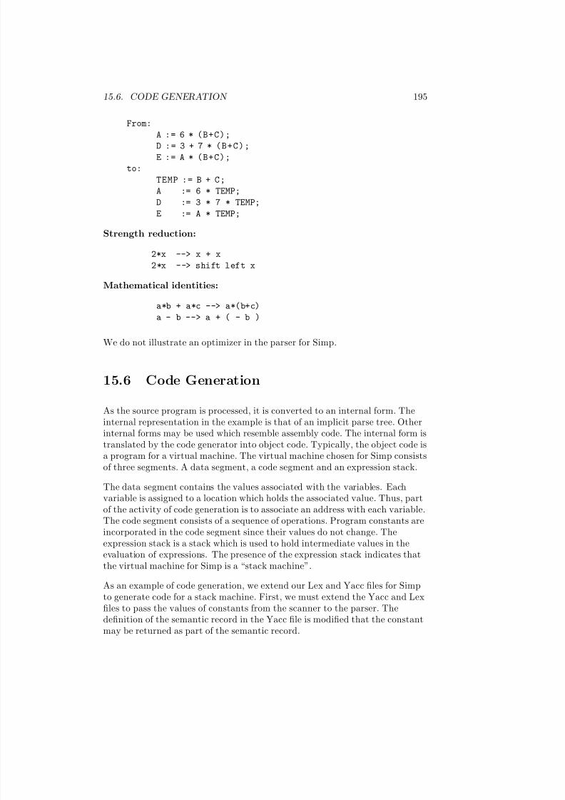
7/3/2019 Theory Introduction to Programming Languages
http://slidepdf.com/reader/full/theory-introduction-to-programming-languages-5584618bb4249 209/233
15.6. CODE GENERATION 195
From:
A := 6 * (B+C);
D := 3 + 7 * (B+C);
E := A * (B+C);
to:
TEMP := B + C;
A := 6 * TEMP;
D := 3 * 7 * TEMP;
E := A * TEMP;
Strength reduction:
2*x --> x + x
2*x --> shift left x
Mathematical identities:
a*b + a*c --> a*(b+c)
a - b --> a + ( - b )
We do not illustrate an optimizer in the parser for Simp.
15.6 Code Generation
As the source program is processed, it is converted to an internal form. The
internal representation in the example is that of an implicit parse tree. Otherinternal forms may be used which resemble assembly code. The internal form istranslated by the code generator into object code. Typically, the object code isa program for a virtual machine. The virtual machine chosen for Simp consistsof three segments. A data segment, a code segment and an expression stack.
The data segment contains the values associated with the variables. Eachvariable is assigned to a location which holds the associated value. Thus, partof the activity of code generation is to associate an address with each variable.The code segment consists of a sequence of operations. Program constants areincorporated in the code segment since their values do not change. Theexpression stack is a stack which is used to hold intermediate values in theevaluation of expressions. The presence of the expression stack indicates thatthe virtual machine for Simp is a “stack machine”.
As an example of code generation, we extend our Lex and Yacc files for Simpto generate code for a stack machine. First, we must extend the Yacc and Lexfiles to pass the values of constants from the scanner to the parser. Thedefinition of the semantic record in the Yacc file is modified that the constantmay be returned as part of the semantic record.
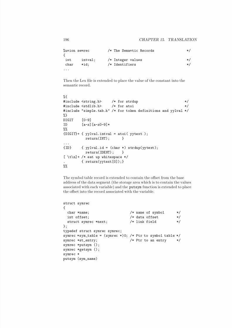
7/3/2019 Theory Introduction to Programming Languages
http://slidepdf.com/reader/full/theory-introduction-to-programming-languages-5584618bb4249 210/233
196 CHAPTER 15. TRANSLATION
%union semrec /* The Semantic Records */
{
int intval; /* Integer values */
char *id; /* Identifiers */
...
Then the Lex file is extended to place the value of the constant into thesemantic record.
%{
#include <string.h> /* for strdup */
#include <stdlib.h> /* for atoi */
#include "simple.tab.h" /* for token definitions and yylval */
%}DIGIT [0-9]
ID [a-z][a-z0-9]*
%%
{DIGIT}+ { yylval.intval = atoi( yytext );
return(INT); }
...
{ID} { yylval.id = (char *) strdup(yytext);
return(IDENT); }
[ \t\n]+ /* eat up whitespace */
. { return(yytext[0]);}
%%
The symbol table record is extended to contain the offset from the baseaddress of the data segment (the storage area which is to contain the valuesassociated with each variable) and the putsym function is extended to placethe offset into the record associated with the variable.
struct symrec
{
char *name; /* name of symbol */
int offset; /* data offset */
struct symrec *next; /* link field */
};
typedef struct symrec symrec;symrec *sym_table = (symrec *)0; /* Ptr to symbol table */
symrec *st_entry; /* Ptr to an entry */
symrec *putsym ();
symrec *getsym ();
symrec *
putsym (sym_name)
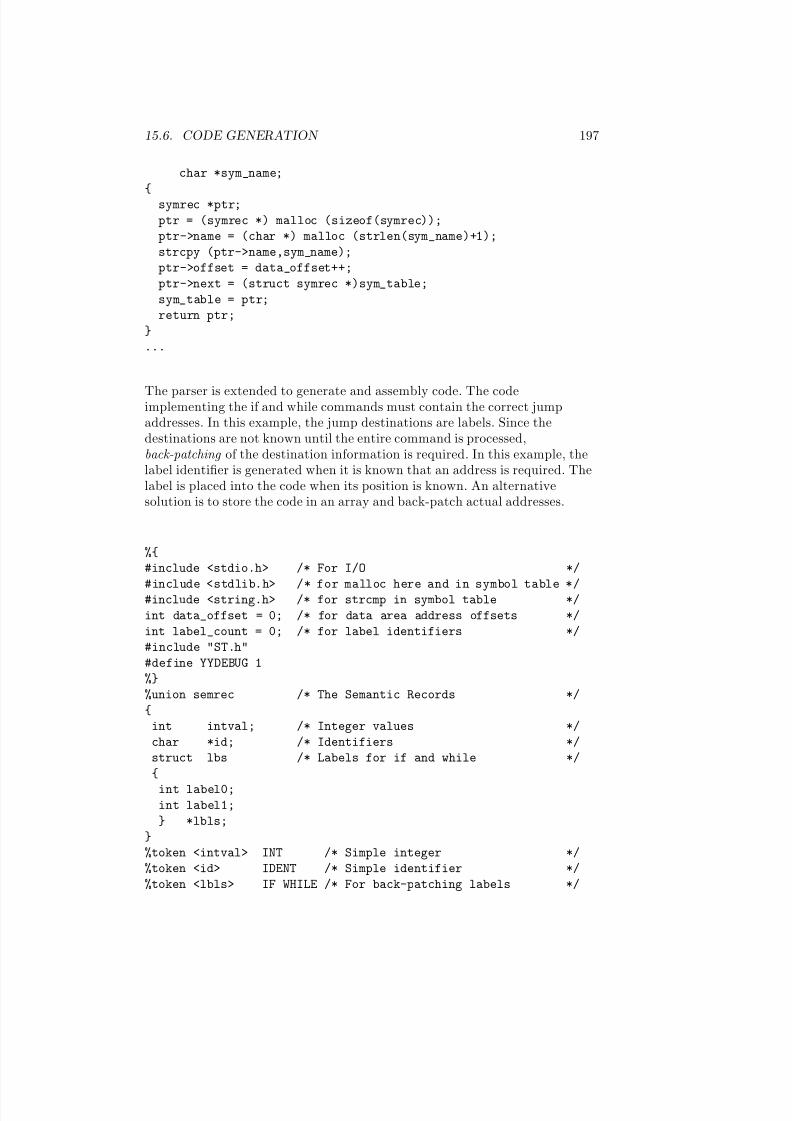
7/3/2019 Theory Introduction to Programming Languages
http://slidepdf.com/reader/full/theory-introduction-to-programming-languages-5584618bb4249 211/233
15.6. CODE GENERATION 197
char *sym_name;
{
symrec *ptr;
ptr = (symrec *) malloc (sizeof(symrec));
ptr->name = (char *) malloc (strlen(sym_name)+1);
strcpy (ptr->name,sym_name);
ptr->offset = data_offset++;
ptr->next = (struct symrec *)sym_table;
sym_table = ptr;
return ptr;
}
...
The parser is extended to generate and assembly code. The codeimplementing the if and while commands must contain the correct jumpaddresses. In this example, the jump destinations are labels. Since thedestinations are not known until the entire command is processed,back-patching of the destination information is required. In this example, thelabel identifier is generated when it is known that an address is required. Thelabel is placed into the code when its position is known. An alternativesolution is to store the code in an array and back-patch actual addresses.
%{
#include <stdio.h> /* For I/O */
#include <stdlib.h> /* for malloc here and in symbol table */#include <string.h> /* for strcmp in symbol table */
int data_offset = 0; /* for data area address offsets */
int label_count = 0; /* for label identifiers */
#include "ST.h"
#define YYDEBUG 1
%}
%union semrec /* The Semantic Records */
{
int intval; /* Integer values */
char *id; /* Identifiers */
struct lbs /* Labels for if and while */
{
int label0;int label1;
} *lbls;
}
%token <intval> INT /* Simple integer */
%token <id> IDENT /* Simple identifier */
%token <lbls> IF WHILE /* For back-patching labels */

7/3/2019 Theory Introduction to Programming Languages
http://slidepdf.com/reader/full/theory-introduction-to-programming-languages-5584618bb4249 212/233
198 CHAPTER 15. TRANSLATION
The semantic record is extended to hold two label identifiers since two labelswill be required for the if and while commands.
The remainder of the file contains the actions associated with code generationfor a stack-machine based architecture.
%token SKIP THEN ELSE FI DO END
%left ’-’ ’+’
%left ’*’ ’/’
%right ’^’ /* Exponentiation */
%%
program : command_sequence { /* print code */ }
;
command_sequence : /* empty */
| command_sequence command ’;’;
command : SKIP
| IDENT ’:’ ’=’ exp { install( $1, IDENT );
printf("assign %ld\n", st_entry->offset ); }
| IF exp { $1 = (struct lbs *) malloc(sizeof(struct lbs));
$1->label0 = label_count++;
printf("jmp_false label %ld\n",$1->label0); }
THEN command_sequence { $1->label1 = label_count++;
printf("goto label %ld\n",$1->label1); }
ELSE { printf("label %ld\n",$1->label0); }
command_sequenceFI { printf("label %ld\n",$1->label1); }
| WHILE { $1 = (struct lbs *) malloc(sizeof(struct lbs));
$1->label0 = label_count++;
printf("label %ld\n", $1->label0); }
exp { $1->label1 = label_count++;
printf("jmp_false label %ld\n",$1->label1); }
DO
command_sequence
END { printf("goto label%ld\n",$1->label0);
printf("label%ld\n",$1->label1); }
;
exp : INT { printf("load_int %ld\n", $1); }| IDENT { if (getsym($1) == 0)
printf("Undefined variable: %s\n", $1);
else
printf("load_var %ld\n", getsym($1)->offset); }
| exp ’<’ exp { printf("less_than%\n"); }
| exp ’=’ exp { printf("equal%\n"); }
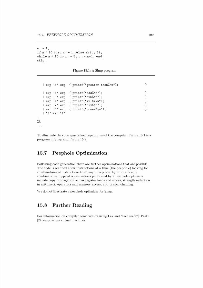
7/3/2019 Theory Introduction to Programming Languages
http://slidepdf.com/reader/full/theory-introduction-to-programming-languages-5584618bb4249 213/233
15.7. PEEPHOLE OPTIMIZATION 199
n := 1;
if n < 10 then x := 1; else skip; fi;
while n < 10 do x := 5; n := n+1; end;
skip;
Figure 15.1: A Simp program
| exp ’>’ exp { printf("greater_than%\n"); }
| exp ’+’ exp { printf("add%\n"); }
| exp ’-’ exp { printf("sub%\n"); }
| exp ’*’ exp { printf("mult%\n"); }| exp ’/’ exp { printf("div%\n"); }
| exp ’^’ exp { printf("power%\n"); }
| ’(’ exp ’)’
;
%%
...
To illustrate the code generation capabilities of the compiler, Figure 15.1 is aprogram in Simp and Figure 15.2.
15.7 Peephole Optimization
Following code generation there are further optimizations that are possible.The code is scanned a few instructions at a time (the peephole) looking forcombinations of instructions that may be replaced by more efficientcombinations. Typical optimizations performed by a peephole optimizerinclude copy propagation across register loads and stores, strength reductionin arithmetic operators and memory access, and branch chaining.
We do not illustrate a peephole optimizer for Simp.
15.8 Further Reading
For information on compiler construction using Lex and Yacc see[27]. Pratt[24] emphasizes virtual machines.
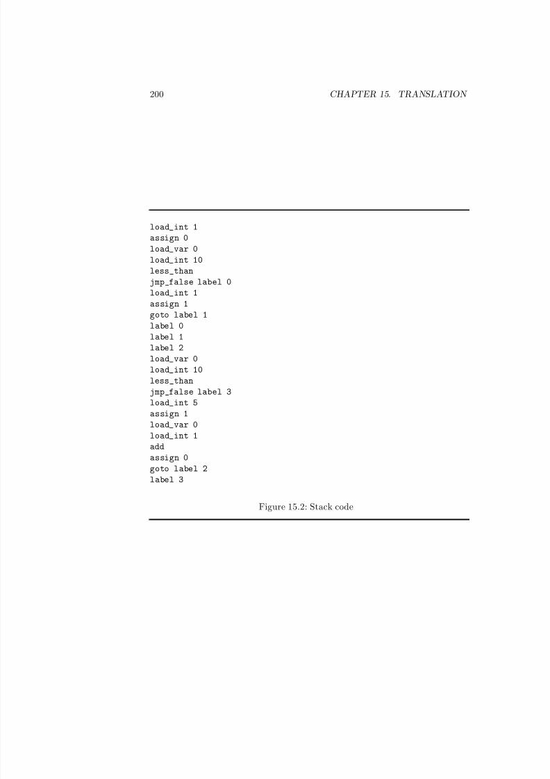
7/3/2019 Theory Introduction to Programming Languages
http://slidepdf.com/reader/full/theory-introduction-to-programming-languages-5584618bb4249 214/233
200 CHAPTER 15. TRANSLATION
load_int 1
assign 0
load_var 0
load_int 10
less_thanjmp_false label 0
load_int 1
assign 1
goto label 1
label 0
label 1
label 2
load_var 0
load_int 10
less_than
jmp_false label 3
load_int 5
assign 1
load_var 0
load_int 1
add
assign 0
goto label 2
label 3
Figure 15.2: Stack code
7/3/2019 Theory Introduction to Programming Languages
http://slidepdf.com/reader/full/theory-introduction-to-programming-languages-5584618bb4249 215/233
Chapter 16
Evaluation of Programming
Languages
16.1 Models of Computation
The first requirement for a general purpose programming languge is that itscomputational model must be universal . That is, every problem that has analgorithmic solution must be solvable in the computational model. Thisrequirement is easily met as the lambda calculus and the imperative model
show.
The computational model must be implementatable on a computer.
Functional Programming:
Logic Programming:
Imperative Programming:
Object-Oriented Programming:
Concurrent Programming:
16.2 Syntax
1 Principle of Simplicity: The language should be based upon as few “basic concepts” as possible.
201
7/3/2019 Theory Introduction to Programming Languages
http://slidepdf.com/reader/full/theory-introduction-to-programming-languages-5584618bb4249 216/233
202 CHAPTER 16. EVALUATION OF PROGRAMMING LANGUAGES
2 Principle of Orthogonality: Independent functions should be controlled by independent mechanisms.
3 Principle of Regularity: A set of objects is said to be regular with respect to some condition if, and only if, the condition is applicable to each element of the set. The basic concepts of the language should be applied consistently and universally.
4 Principle of Type Completeness: There should be no arbitraryrestriction on the use of the types of values. All types have equal status. For example, functions and procedures should be able to have any type asparameter and result. This is also called the principle of regularity.
5 Principle of Parameterization: A formal parameter to an abstract may be from any syntactic class.
6 Principle of Analogy: An analogy is a conformation in pattern between unrelated objects. Analogies are generalizations which are formed when constants are replaced with variables resulting in similarities in structure.Analogous operations should be performed by the same code parameterized by the type of the objects.
7 Principle of Correspondence: For each form of definition there exists a corresponding parameter mechanism and vice versa.
16.3 Semantics
8 Principle of Clarity: The mechanisms used by the language should bewell defined, and the outcome of a particular section of code easily predicted.
9 Principle of Referential Transparency: Any part of a syntactic classmay be replaced with an equal part without changing the meaning of thesyntactic class (substitutivity of equals for equals).
10 Principle of Sub-types: A sub-type may appear wherever an element of the super-type is expected.
16.4 Pragmatics
• Naturalness for the application (relations, functions, objects, processes)
7/3/2019 Theory Introduction to Programming Languages
http://slidepdf.com/reader/full/theory-introduction-to-programming-languages-5584618bb4249 217/233
16.4. PRAGMATICS 203
• Support for abstraction
• Ease of program verification
• Programming environment (editors, debuggers, verifiers, test datagenerators, pretty printers, version control)
• Operating Environment (batch, interactive, embedded-system)
• Portability
• Cost of use (execution, translation, programming, maintenance)
Applicability
11 Principle of Expressivity: The language should allow us to construct as wide a variety of programs as possible.
12 Principle of Extensibility: New objects of each syntactic class may beconstructed (defined) from the basic and defined constructs in a systematicway.
Example: user defined data types, functions and procedures.
Binding, Scope, Lifetime,
Safety
13 Principle of Safety: Mechanisms should be available to allow errors tobe detected.
Type checking-static and dynamic, range checking
14 Principle of the Data Invariant: A data invariant is a property of an object that holds whenever control is not in the object. Objects should bedesigned around a data invariant.
15 Principle of Information Hiding: Each “basic program unit” should only have access to the information that it requires.
16 Principle of Explicit Interfaces: Interfaces between basic program units should be stated explicitly.
7/3/2019 Theory Introduction to Programming Languages
http://slidepdf.com/reader/full/theory-introduction-to-programming-languages-5584618bb4249 218/233
204 CHAPTER 16. EVALUATION OF PROGRAMMING LANGUAGES
17 Principle of Privacy: The private members of a class are inaccessible from code outside the class.
Abstraction
18 Principle of Abstraction: Abstraction is an emphasis on the idea,qualities and properties rather than the particulars (a suppression of detail).An abstract is a named syntactic construct which may be invoked by mentioning the name. Each syntactic class may be referenced as an abstraction. Functions and procedures are abstractions of expressions and commands respectively and there should be abstractions over declarations(generics) and types (parameterized types). Abstractions permit the
suppression of detail by encapsulation or naming. Mechanisms should beavailable to allow recurring patterns in the code to be factored out.
19 Principle of Qualification: A block may be introduced in each syntacticclass for the purpose of admitting local declarations. For example, block commands, block expressions, block definitions.
20 Principle of Representation Independence: A program should bedesigned so that the representation of an object can be changed without affecting the rest of the program.
Generalization
21 Principle of Generalization: Generalization is a broadening of application to encompass a larger domain of objects of the same or different type. Each syntactic class may be generalized by replacing a constituent element with a variable. The idea is to enlarge of domain of applicability of a construct. Mechanisms should be available to allow analogous operations to beperformed by the same code.
polymorphism, overloading, generics
Implementation
22 Principle of Efficiency: The language should not preclude theproduction of efficient code. It should allow the programmer to provide thecompiler with any information which may improve the resultant code.
7/3/2019 Theory Introduction to Programming Languages
http://slidepdf.com/reader/full/theory-introduction-to-programming-languages-5584618bb4249 219/233
16.5. TRENDS IN PROGRAMMING LANGUAGE DESIGN 205
23 Principle of Modularity: Objects of each syntactic class may becompiled separately from the rest of the program.
Novice users of a programming language require language tutorials whichprovide examples and intuitive explanations. More sophisticated users requirereference manuals which catalogue all the features of a programming language.Even more sophisticated students of a programming language require completeand formal descriptions which eliminate all ambiguity from the languagedescription.
16.5 Trends in Programming Language Design
streams, lazy evaluation, reactive systems, knowledge based systems,concurrency, efficient logic and functional languages, OOP.

7/3/2019 Theory Introduction to Programming Languages
http://slidepdf.com/reader/full/theory-introduction-to-programming-languages-5584618bb4249 220/233
206 CHAPTER 16. EVALUATION OF PROGRAMMING LANGUAGES

7/3/2019 Theory Introduction to Programming Languages
http://slidepdf.com/reader/full/theory-introduction-to-programming-languages-5584618bb4249 221/233
Chapter 17
History
17.1 Functional Programming
LISP (LISt Processing) was designed by John McCarthy in 1958. LISP grewout of interest in symbolic computation. In particular, interest in areas such asmechanizing theorem proving, modeling human intelligence, and naturallanguage processing. In each of these areas, list processing was seen as afundamental requirement. LISP was developed as a system for list processingbased on recursive functions. It provided for recursion, first-class functions,and garbage collection. All new concepts at the time. LISP was inadvertantlyimplemented with dynamic rather than static scope rules. Scheme is a modernincarnation of LISP. It is a relatively small language with static rather thandynamic scope rules. LISP was adopted as the language of choice for artificialintelligence applications and continues to be in wide use in the aritficialintelligence community.
ML
Miranda
Haskell is a modern language named after the logician Haskell B. Curry, anddesigned by a 15-member international committee. The design goals forHaskell are have a functional language which incorporates all recent “goodideas” in functional language research and which is suitable for for teaching,research and application. Haskell contains an overloading facility which isincorporated with the polymorphic type system, purely functional i/o, arrays,data abstraction, and information hiding.
207

7/3/2019 Theory Introduction to Programming Languages
http://slidepdf.com/reader/full/theory-introduction-to-programming-languages-5584618bb4249 222/233
208 CHAPTER 17. HISTORY
17.2 Logic Programming
1969 J Robinson and Resolution 1972 Alain Colmerauer
17.3 Imperative Programming
Imperative languages have a rich and varied history. The first imperativeprogramming languages were machine instructions. Machine instructions weresoon replaced with Assembly languages, essentially transliterations of machinecode.
FORTRAN (FORmula TRANslation) was the first high level language to gainwide acceptance. It was designed for scientific applications and featured analgebraic notation, types subprograms and formatted input/output. It wasimplemented in 1956 by John Backus at IBM specifically for the IBM 704machine. Efficient execution was a major concern consequently, its structureand commands have much in common with assembly languages. FORTRANwon wide acceptance and continues to be in wide use in the scientificcomputing community.
COBOL (COmmon Business Oriented Language) was designed (by acommittee of representatives of computer manufactures and the Department of Defense) at the initiative of the U. S. Department of Defense in 1959 andimplemented in 1960 to meet the need for business data processing
applications. COBOL featured records, files and fixed decimal data. It alsoprovided a “natural language” like syntax so that programs would be able tobe read and understood by non-programmers. COBOL won wide acceptancein the business data processing community and continues to be in wide use.
ALGOL 60 (ALGorithmic Oriented Language) was designed in 1960 by aninternational committee for use in scientific problem solving. UnlikeFORTRAN it was designed independently of an implementation, a choicewhich lead to an elegant language. The description of ALGOL 60 introducedthe BNF notation for the definition of syntax and is a model of clarity andcompleteness. Although ALGOL 60 failed to win wide acceptance, itintroduced block structure, structured control statements and recursiveprocedures into the imperative programming paradigm.
PL/I (Programming Languge I) was developed at IBM in the mid 1960s. Itwas designed as a general purpose language to replace the specific purposelanguages like FORTRAN, ALGOL 60, COBOL, LISP, and APL (APL andLISP were consdered in chapter 7). PL/I incorporated block structure,structured control statements, and recursion from ALGOL 60, subprogramsand formatted input/output from FORTRAN, file manipulation and the
7/3/2019 Theory Introduction to Programming Languages
http://slidepdf.com/reader/full/theory-introduction-to-programming-languages-5584618bb4249 223/233
17.4. CONCURRENT PROGRAMMING 209
record structure from COBOL, dynamic storage allocation and linkedstructures from LISP, and some array operations from APL. PL/I introducedexception handling and multitasking for concurrent programming. PL/I wascomplex, difficult to learn, and difficult to implement. For these and otherreasons PL/I failed to win wide acceptance.
Simula 67
ALGOL 68 was designed to be a general purpose language which remediedPL/I’s defects by using a small number of constructs and rules for combiningthe any of the constructs with predictable results–orthogonality. Thedescription of ALGOL 68 issued in 1969 was difficult to understand since itintroduced a notation and terminology that was foreign to the computingcommunity. ALGOL 68 introduced orthogonality and data extensibility as a
way to produce a compact but powerful language. The “ALGOL 68 Report”considered to be one of the most unreadable documents ever printed andimplementation difficulties prevented ALGOL 68’s acceptance.
Pascal was developed partly as a reaction to the problems encountered withALGOL 68 and as an attempt to provide a small and efficient implementationof a language suitable for teaching good programming style.
C is an attempt to provide an efficient language for systems programming.
Modula-2
Ada was developed as the result of a Department of Defense initiative. LikePL/1 and Algol-68, Ada represents an attempt to produce a complete
langauge representing the full range of programming tasks.
17.4 Concurrent Programming
17.5 Object-Oriented Programming

7/3/2019 Theory Introduction to Programming Languages
http://slidepdf.com/reader/full/theory-introduction-to-programming-languages-5584618bb4249 224/233
210 CHAPTER 17. HISTORY
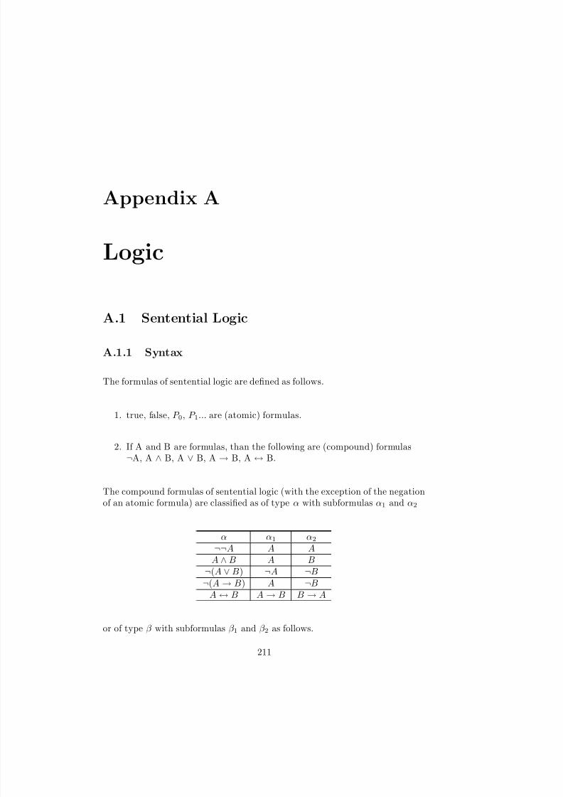
7/3/2019 Theory Introduction to Programming Languages
http://slidepdf.com/reader/full/theory-introduction-to-programming-languages-5584618bb4249 225/233
Appendix A
Logic
A.1 Sentential Logic
A.1.1 Syntax
The formulas of sentential logic are defined as follows.
1. true, false, P 0, P 1... are (atomic) formulas.
2. If A and B are formulas, than the following are (compound) formulas¬A, A ∧ B, A ∨ B, A → B, A ↔ B.
The compound formulas of sentential logic (with the exception of the negationof an atomic formula) are classified as of type α with subformulas α1 and α2
α α1 α2
¬¬A A A
A ∧ B A B¬(A ∨ B) ¬A ¬B
¬(A → B) A ¬BA ↔ B A → B B → A
or of type β with subformulas β 1 and β 2 as follows.
211
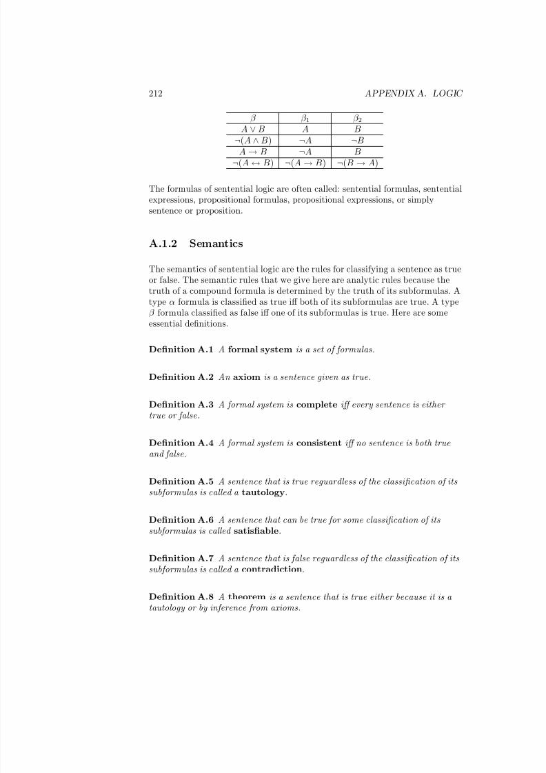
7/3/2019 Theory Introduction to Programming Languages
http://slidepdf.com/reader/full/theory-introduction-to-programming-languages-5584618bb4249 226/233
212 APPENDIX A. LOGIC
β β 1 β 2A ∨ B A B
¬(A ∧ B) ¬A ¬BA → B ¬A B
¬(A ↔ B) ¬(A → B) ¬(B → A)
The formulas of sentential logic are often called: sentential formulas, sententialexpressions, propositional formulas, propositional expressions, or simplysentence or proposition.
A.1.2 Semantics
The semantics of sentential logic are the rules for classifying a sentence as trueor false. The semantic rules that we give here are analytic rules because thetruth of a compound formula is determined by the truth of its subformulas. Atype α formula is classified as true iff both of its subformulas are true. A typeβ formula classified as false iff one of its subformulas is true. Here are someessential definitions.
Definition A.1 A formal system is a set of formulas.
Definition A.2 An axiom is a sentence given as true.
Definition A.3 A formal system is complete iff every sentence is either true or false.
Definition A.4 A formal system is consistent iff no sentence is both trueand false.
Definition A.5 A sentence that is true reguardless of the classification of itssubformulas is called a tautology.
Definition A.6 A sentence that can be true for some classification of itssubformulas is called satisfiable.
Definition A.7 A sentence that is false reguardless of the classification of itssubformulas is called a contradiction.
Definition A.8 A theorem is a sentence that is true either because it is a tautology or by inference from axioms.
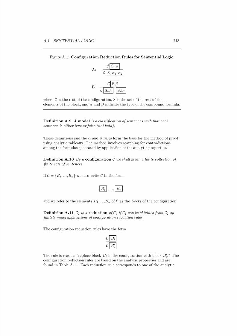
7/3/2019 Theory Introduction to Programming Languages
http://slidepdf.com/reader/full/theory-introduction-to-programming-languages-5584618bb4249 227/233
A.1. SENTENTIAL LOGIC 213
Figure A.1: Configuration Reduction Rules for Sentential Logic
A:C S, α
C S, α1, α2
B:C S,β
C S,β 1 , S,β 2
where C is the rest of the configuration, S is the set of the rest of theelements of the block, and α and β indicate the type of the compound formula.
Definition A.9 A model is a classification of sentences such that each sentence is either true or false (not both).
These definitions and the α and β rules form the base for the method of proof using analytic tableaux. The method involves searching for contradictionsamong the formulas generated by application of the analytic properties.
Definition A.10 By a configuration C we shall mean a finite collection of finite sets of sentences.
If C = {B1,...,Bn} we also write C in the form
B1 ,..., Bn
and we refer to the elements B1,...,Bn of C as the blocks of the configuration.
Definition A.11 C2 is a reduction of C1 if C2 can be obtained from C2 by finitely many applications of configuration reduction rules.
The configuration reduction rules have the form
C Bi
C B
i
The rule is read as “replace block Bi in the configuration with block B
i.” Theconfiguration reduction rules are based on the analytic properties and arefound in Table A.1. Each reduction rule corresponds to one of the analytic

7/3/2019 Theory Introduction to Programming Languages
http://slidepdf.com/reader/full/theory-introduction-to-programming-languages-5584618bb4249 228/233
214 APPENDIX A. LOGIC
properties. Given a block with a formula of type α or β the reduction rulesspecify the replacement of a block with one or more blocks in which theformula is replaced with its subformulas. For example, rule A permits thereplacement of a conjunction with the conjuncts and rule B requires the blockto be replaced with two blocks each containing one of the disjuncts.
The configuration reduction rules may be used to construct a model underwhich a given formula is satisfiable. For example, the configuration reductionrules generate the following sequence of configurations given the propositionalformula, ¬[( p ∨ q) → ( p ∧ q)].
¬[( p ∨ q) → ( p ∧ q)]
( p ∨ q), ¬( p ∧ q)
p, ¬( p ∧ q) , q, ¬( p ∧ q)
p, ¬ p , p, ¬q , q, ¬ p , q, ¬q
Note that the outer two blocks of the last line are contradictory and the innertwo define an interpretation under which the formula is satisfiable.
A.2 Predicate Logic
Predicate Logic (or Predicate Calculus or First-Order Logic) is a generalizationof Sentential Logic. Generalization requires the introduction of variables andthe variables of Predicate Logic are of two kinds: free and bound.
A.2.1 Syntax
1. A sentence is also a predicate with no free variables.
2. If p is a predicate and x is a variable but not a variable in p and T is atype then the following are also predicates. ∀x.T : p(x) and ∃x.T : p(x)which have the same free variables as p but have in addition the bound
variable x. p(x) is formed from p by replacing any number of occurrencesof some constant of type T in p with x. x is said to be free in p(x) and issaid to be bound in ∀x.T : p(x) and ∃x.T : p(x).
The additional formulas of Predicate Logic are compound formulas and theuniversally quantified formulas are of type γ with subformula γ (c). A type γ formula holds iff its subformula holds for each constant of the appropriate type.
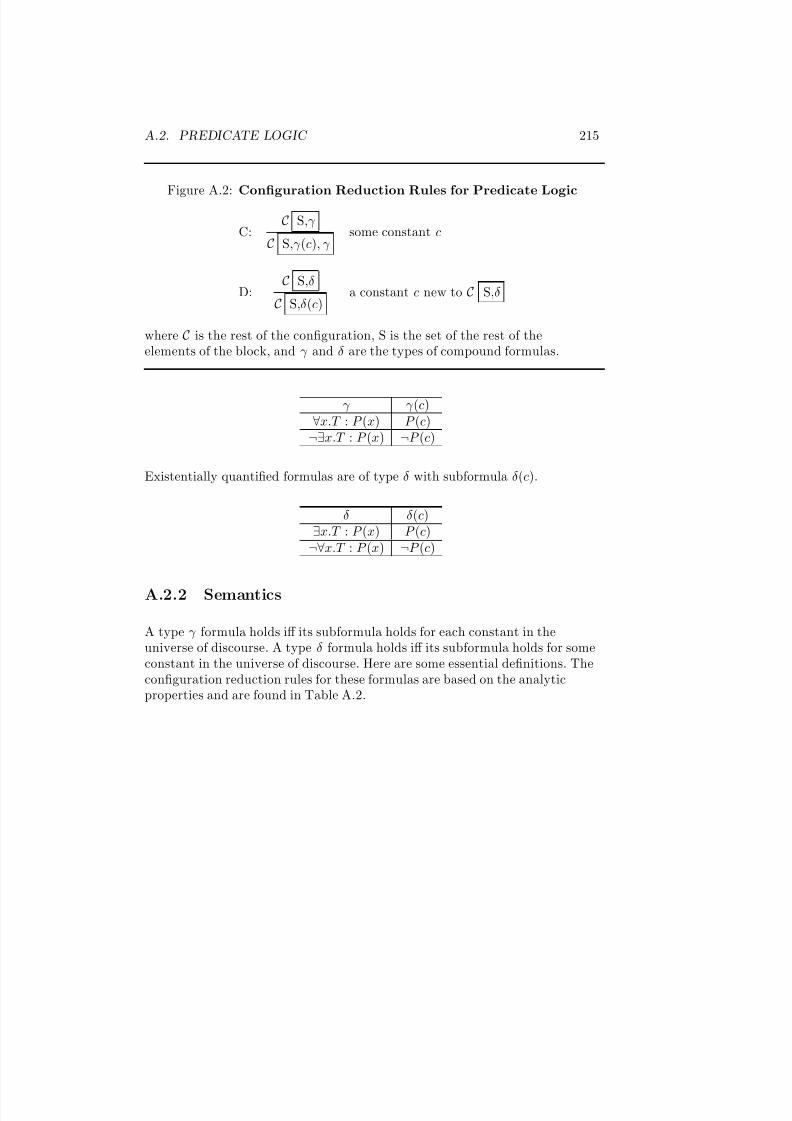
7/3/2019 Theory Introduction to Programming Languages
http://slidepdf.com/reader/full/theory-introduction-to-programming-languages-5584618bb4249 229/233
A.2. PREDICATE LOGIC 215
Figure A.2: Configuration Reduction Rules for Predicate Logic
C:C S,γ
C S,γ (c), γ some constant c
D:C S,δ
C S,δ(c)a constant c new to C S,δ
where C is the rest of the configuration, S is the set of the rest of theelements of the block, and γ and δ are the types of compound formulas.
γ γ (c)∀x.T : P (x) P (c)
¬∃x.T : P (x) ¬P (c)
Existentially quantified formulas are of type δ with subformula δ(c).
δ δ(c)∃x.T : P (x) P (c)
¬∀x.T : P (x) ¬P (c)
A.2.2 Semantics
A type γ formula holds iff its subformula holds for each constant in theuniverse of discourse. A type δ formula holds iff its subformula holds for someconstant in the universe of discourse. Here are some essential definitions. Theconfiguration reduction rules for these formulas are based on the analyticproperties and are found in Table A.2.

7/3/2019 Theory Introduction to Programming Languages
http://slidepdf.com/reader/full/theory-introduction-to-programming-languages-5584618bb4249 230/233
216 APPENDIX A. LOGIC

7/3/2019 Theory Introduction to Programming Languages
http://slidepdf.com/reader/full/theory-introduction-to-programming-languages-5584618bb4249 231/233
Bibliography
[1] Abelson, H., Sussman, G.J., and Sussman, J. Structure and Interpretation
of Computer Programs. MIT Press, Cambridge, Massachusetts, 1985.
[2] Backus, J. W., “Can Programming Be Liberated from the von NeumannStyle?” CACM, vol. 21, no. 8, pp. 613-614.
[3] Barendregt, H. P., The Lambda Calculus: Its Syntax and Semantics. 2ded. North-Holland, 1984.
[4] Bird, R.A. and Wadler, P.L., Introduction to Functional Programming .Prentice/Hall International, 1988.
[5] Boehm, C. and Jacopini, G., “Flow Diagrams, Turnign Machines, andLanguages with Only Two Foramation Rules.” CACM, vol. 9, no. 5, pp.366-371.
[6] Curry. H. B. and Feys, R., Combinatory Logic, Vol. I. North-Holland,1968.
[7] Curry. H. B., Hindley, J. R., and Seldin, J. P., Combinatory Logic, Vol. II.North-Holland, 1972.
[8] Deransart, P., Jourdan, M., and Lorho, B., Attribute Grammars:Definitions, Systems and Bibliography . Lecture Notes in ComputerScience 323. Springer-Verlag, 1988.
[9] Dijkstra, E. W., “Goto Statement Considered Harmful.” Communicationsof the ACM vol. 11 no. 5 (May 1968): pp. 147-149.
[10] Gries, D., The Science of Programming Springer-Verlag, New York, 1981.
[11] Hehner, E. C. R., The Logic of Programming . Prentice/Hall International,1984.
[12] Henderson, Peter, Functional Programming: Application and Implementation . Prentice/Hall International, 1980.
217
7/3/2019 Theory Introduction to Programming Languages
http://slidepdf.com/reader/full/theory-introduction-to-programming-languages-5584618bb4249 232/233
218 BIBLIOGRAPHY
[13] Hindley, J. R., and Seldin, J. P., Introduction to Combinators and λCalculus, Cambridge University Press, London, 1986.
[14] Hopcroft, J. E. and Ullman, J. D., Introduction to Automata Theory,Languages and Computation . Addison-Wesley, 1979.
[15] Knuth, D. E., “Semantics of context-free languages.” MathematicalSystems Theory, vol. 2, 1968, pp. 127-145. Correction in MathematicalSystems Theory, vol. 5, 1971, p. 95.
[16] Kowalski, R. A., “Algorithm = Logic + Control”. CACM vol. 22 no. 7,pp. 424-436, 1979.
[17] Landin, P. J., The next 700 programming languages, Communications of the ACM 9, 157-64 1966.
[18] McCarthy, J., “Recursive functions of symbolic expressions and theircomputation by machine, Part I.” CACM vol. 3 no. 4, pp. 184-195, 10,1960.
[19] McCarthy, J., Abrahams, P. W., Edwards, D. J., Hart, T. P., and Levin,M., LISP 1.5 Programmer’s Manual . 2d ed. MIT Press, Cambridge, MA.1965.
[20] MacLennan, Bruce J., Functional programming: practice and theory .Addison-Wesley Publishing Company, Inc. 1990.
[21] Miller, G. A., The Psychology of Communication . Basic Books, New York,1967.
[22] Peyton Jones, Simon L., The Implementation of Functional Programming Languages. Prentice/Hall International, 1987.
[23] Pittman, T. and Peters, J., The Art of Compiler Design: Theory and Practice. Prentice-Hall, 1992.
[24] Pratt, T. W., Programming Languages: Design and Implementation .Printice-Hall, 1984.
[25] Revesz, G, E., Lambda-Calculus, Combinators, and Functional Programming . Cambridge University Press, Cambridge, 1988.
[26] Schmidt, D. A., Denotational Semantics: A Methodology for LanguageDevelopment . Wm. C. Brown, Dubuque, Iowa, 1988.
[27] Schreiner, A. T. and Freidman, H. G., Introduction to Compiler Construction with Unix Prentice-Hall, 1985.
[28] Scott, D. S., Denotational Semantics: The Scott-Strachey Approach toProgramming Language Theory . MIT Press, 1987.
7/3/2019 Theory Introduction to Programming Languages
http://slidepdf.com/reader/full/theory-introduction-to-programming-languages-5584618bb4249 233/233
BIBLIOGRAPHY 219
[29] Steele, G. L., Jr., Common Lisp. Digital Press, Burlington, MA. 1984.
[30] Tennent, R. D., Principles of Programming Languages, Prentice-HallInternational, 1981.
[31] Wegner, Peter, “Concepts and Paradigms of Object-OrientedProgramming.” OOPS Messenger vol. 1 no. 1 (August 1990): pp. 7-87.
[32] Worf, Benjamin, Language thought and reality, MIT Press, CambridgeMass., 1956.