theory verification methodology - emucivil.emu.edu.tr/courses/civl455/4-theory of software.pdf ·...
TRANSCRIPT
The theoretical part of help contains all theoretical basis employed in computations with our programs.
The program allows for structure verification according to three methodologies:
� Verification according to EN 1997 � Verification according to LRFD � Classical analysis employing verification according to limit states or safety factors,
respectively
The actual calculations (e.g., pressure calculation, determination of bearing capacity of foundation soil) are the same for all three methodologies – they differ only in the way of introducing the design coefficients, combinations and the procedure for verifying the structure reliability.
When adopting the classical approach it is possible to model the structure using in general any type of standard and therefore also EN 1997 or LRFD – for significant complexity of these methods, however, the program was enhanced to allow for their direct application.
Designing a structure according to EN 1997-1 is based on the analysis of limit states.
The stepping stone for a safe design is a correct settings of partial factors for the selected "National Annex" or "Design approach", respectively.
Partial factors are identical for analyses in given program, for individual stages it also possible to choose a "Design situation".
The programs can be grouped into several categories based on the analysis approach and the degree on automation:
� Analysis of walls, supporting structures (walls, abutment, nailed slopes) � Analysis of sheeting structures (sheeting design, sheeting check, earth pressure) � Foundation analysis (spread footing, pile) � Slope stability analysis
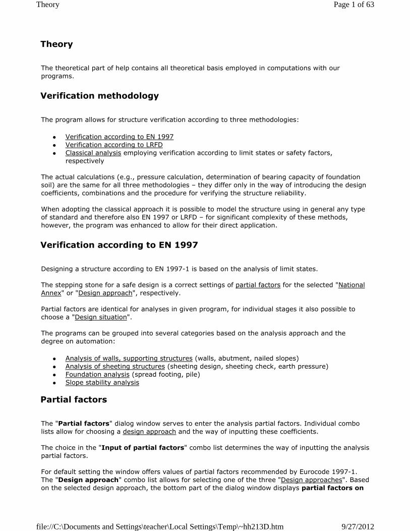
The "Partial factors" dialog window serves to enter the analysis partial factors. Individual combo lists allow for choosing a design approach and the way of inputting these coefficients.
The choice in the "Input of partial factors" combo list determines the way of inputting the analysis partial factors.
For default setting the window offers values of partial factors recommended by Eurocode 1997-1. The "Design approach" combo list allows for selecting one of the three "Design approaches". Based on the selected design approach, the bottom part of the dialog window displays partial factors on
Theory
Verification methodology
Verification according to EN 1997
Partial factors
Page 1 of 63Theory
9/27/2012file://C:\Documents and Settings\teacher\Local Settings\Temp\~hh213D.htm
action, material or resistance, respectively, and combination factors for variable actions. In such a case the values of partial factors cannot be modified. A partial factor adjusting the action of water is an exception.
The user setting allows for specifying arbitrary values of partial factors. Default values, according to national annexes, can be copied into the user values by pressing the "Take over values" button.
Furthermore, it is also possible to choose individual EU countries – the window then displays partial factors corresponding to the selected national annexes (NA). In most cases, only one Design approach is then allowed based on NAD and the program (the type of the analyzed geotechnical task).
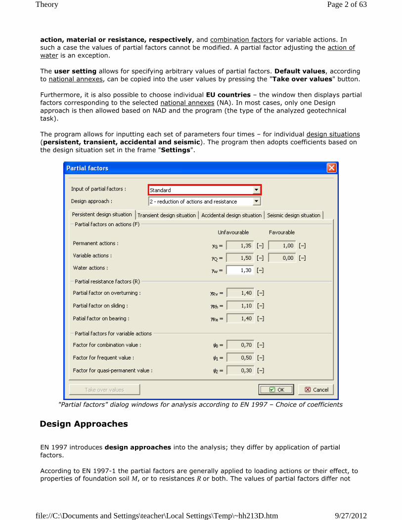
The program allows for inputting each set of parameters four times – for individual design situations (persistent, transient, accidental and seismic). The program then adopts coefficients based on the design situation set in the frame "Settings".
"Partial factors" dialog windows for analysis according to EN 1997 – Choice of coefficients
EN 1997 introduces design approaches into the analysis; they differ by application of partial factors.
According to EN 1997-1 the partial factors are generally applied to loading actions or their effect, to properties of foundation soil M, or to resistances R or both. The values of partial factors differ not
Design Approaches
Page 2 of 63Theory
9/27/2012file://C:\Documents and Settings\teacher\Local Settings\Temp\~hh213D.htm

only by the assumed design approach, but also by the type of geotechnical task (support structures, pile, etc.). The values of partial factors are in general specified by Eurocode in Annexes A; the national choice of values of partial factors specifies NA. The program automatically displays the required coefficients depending on the selected design approach (or possible according to National Annex).
Regarding the fact that individual Design approaches introduce the partial factors into the analysis in a different way, it is logical that the results attributed to these design approaches may also considerably differ. If National Annex does not recommend for a given geotechnical task a Design approach, it is up to the designer to select it (and therefore also to evaluate whether the results correspond to the analyzed situation).
� Design approach 1 – Verification is performed for two sets of coefficients (Combination 1 and Combination 2) used in two separate analyses. Coefficients are applied to loading actions and to material parameters.
� Design approach 2 – Applies partial factors to loading actions and material resistance (bearing capacity).
� Design approach 3 – Applies partial factors to loading actions and at the same type to material (material parameters of soil).
"Partial factors" dialog windows for analysis according to EN 1997 – Choice of design approach
Page 3 of 63Theory
9/27/2012file://C:\Documents and Settings\teacher\Local Settings\Temp\~hh213D.htm

It is used in UK and Portugal.
Verification is performed for two sets of coefficients (Combination 1 and Combination 2) used in two separate analyses. For combination 1 the partial factors are applied to loading actions only, the remaining coefficients are equal to zero. For combination 2 the partial factors are applied to material parameters (material parameters of soil) and to variable loading actions, the remain coefficients are equal to 1,0.
In programs analyzing walls the analysis is carried out for both combinations automatically and the results are presented for the most severe situation. Detailed description of the results for both combinations is available in the output protocol.
This approach is not applicable for programs "Sheeting check" and "Slope stability". The combination, for which the analysis should be carried out, must be selected in the "Partial factors" dialog window.
Programs "Spread footing" and "Pile" require specifying the combination number for the inputted load – the analysis then adopts the corresponding partial factors based on the type of combination.
Design approach 1
Page 4 of 63Theory
9/27/2012file://C:\Documents and Settings\teacher\Local Settings\Temp\~hh213D.htm

Default values recommended by EN 1997-1 for design approach 1
It is used in most countries EU (Germany, Slovakia, Italy...).
The design approach 2 applies the partial factors to loading actions and to material resistance (bearing capacity).
Default values recommended by EN 1997-1 for design approach 2
It is used in the Netherlands and further in most countries for the slope stability analysis.
The design approach 3 applies the partial factors to loading actions and at the same type to material (material parameters of soil).
Compare to other design approaches it extends geotechnical loads – State GEO (loading attributed to soils – e.g. earth pressures, pressures due to a surcharge, water action) and loads applied to structures – State STR (the program considers the self weight of a structure, inputted forces acting on a structure, anchors, geo-reinforcements, mesh overhangs). A different set of coefficients, specified in the "Partial factors" dialog window, is used for each type of loading. Partial factors applied to geotechnical loads are mostly smaller than those applied to structure loads.
Design approach 2
Design approach 3
Page 5 of 63Theory
9/27/2012file://C:\Documents and Settings\teacher\Local Settings\Temp\~hh213D.htm

Default values recommended by EN 1997-1 for design approach 3
The program allows for choosing a national annex in the "Partial factors" dialog window.
National Annex (NA)
Page 6 of 63Theory
9/27/2012file://C:\Documents and Settings\teacher\Local Settings\Temp\~hh213D.htm

"Partial factors" dialog window – choice of National Annex
National annex (NA) offers in detail how to apply Eurocode on national level (in individual EU countries) and it was usually issued together with ENV of a given country.
The National Annex therefore determines the choice of partial factors on national level and application of Design approaches for individual geotechnical tasks. Owing to the fact that content of NA remains open in some member countries, not all national annexes are implemented into individual programs yet.
Our goal is to continuously update the list of national annexes. Therefore we appreciate any information from users from individual EU countries (to that end use email [email protected]).
Programs allow for defining four design situations in the frame "Settings".
� Persistent – considers actions acting on the structure during the assumed lifetime (conventional service of a structure).
� Transient – considers actions acting on the structure over a short time interval (e.g. load actions attributed to construction).
� Accidental – considers exceptional actions on a structure (e.g. blast, vehicle impact, flood, etc.).
� Seismic – considers actions on a structure during seismic activity.
Design situations determine which set of partial factors will be used in the analysis. Selection of design situation makes it possible to change partial factors in individual stages of calculation within one task.
Partial factors adjusting the load action of water can be modified in the "Partial factors" dialog window for all variants of input. The partial factor on influence of water adjusts the magnitude of force due to water action; the magnitude of pore pressure respectively.
Design situation
Partial factors on water
Page 7 of 63Theory
9/27/2012file://C:\Documents and Settings\teacher\Local Settings\Temp\~hh213D.htm
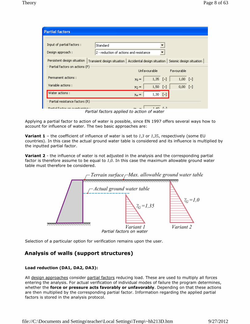
Partial factors applied to action of water
Applying a partial factor to action of water is possible, since EN 1997 offers several ways how to account for influence of water. The two basic approaches are:
Variant 1 – the coefficient of influence of water is set to 1,3 or 1,35, respectively (some EU countries). In this case the actual ground water table is considered and its influence is multiplied by the inputted partial factor.
Variant 2 - the influence of water is not adjusted in the analysis and the corresponding partial factor is therefore assume to be equal to 1,0. In this case the maximum allowable ground water table must therefore be considered.
Partial factors on water
Selection of a particular option for verification remains upon the user.
Load reduction (DA1, DA2, DA3):
All design approaches consider partial factors reducing load. These are used to multiply all forces entering the analysis. For actual verification of individual modes of failure the program determines, whether the force or pressure acts favorably or unfavorably. Depending on that these actions are then multiplied by the corresponding partial factor. Information regarding the applied partial factors is stored in the analysis protocol.
Analysis of walls (support structures)
Page 8 of 63Theory
9/27/2012file://C:\Documents and Settings\teacher\Local Settings\Temp\~hh213D.htm
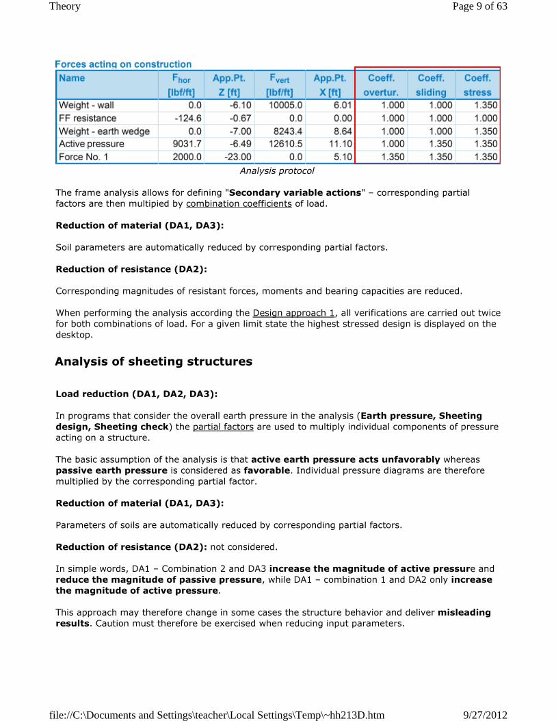
Analysis protocol
The frame analysis allows for defining "Secondary variable actions" – corresponding partial factors are then multipied by combination coefficients of load.
Reduction of material (DA1, DA3):
Soil parameters are automatically reduced by corresponding partial factors.
Reduction of resistance (DA2):
Corresponding magnitudes of resistant forces, moments and bearing capacities are reduced.
When performing the analysis according the Design approach 1, all verifications are carried out twice for both combinations of load. For a given limit state the highest stressed design is displayed on the desktop.
Load reduction (DA1, DA2, DA3):
In programs that consider the overall earth pressure in the analysis (Earth pressure, Sheeting design, Sheeting check) the partial factors are used to multiply individual components of pressure acting on a structure.
The basic assumption of the analysis is that active earth pressure acts unfavorably whereas passive earth pressure is considered as favorable. Individual pressure diagrams are therefore multiplied by the corresponding partial factor.
Reduction of material (DA1, DA3):
Parameters of soils are automatically reduced by corresponding partial factors.
Reduction of resistance (DA2): not considered.
In simple words, DA1 – Combination 2 and DA3 increase the magnitude of active pressure and reduce the magnitude of passive pressure, while DA1 – combination 1 and DA2 only increase the magnitude of active pressure.
This approach may therefore change in some cases the structure behavior and deliver misleading results. Caution must therefore be exercised when reducing input parameters.
Analysis of sheeting structures
Page 9 of 63Theory
9/27/2012file://C:\Documents and Settings\teacher\Local Settings\Temp\~hh213D.htm

Response of sheeting structure upon unloading
Load reduction (DA1, DA2, DA3):
Loading on foundation is taken as a result of the analysis of upper structure.
� load cases are determined according to rules provided by EN 1990:2002 � combinations of load cases are calculated according to EN 1991
The results of calculated combinations the serve as an input into programs Spread footing and Pile.
Either design (bearing capacity analysis, dimensioning of footing) or service (analysis of settlement) load is considered. In Design approach 1, analysis is performed for both, inputted design load (combination 1) as well as inputted service load (combination 2).
Only the structure self-weigh or the weight of soil above footing is multiplied by partial factors in the program. The specified design load must be determined in accord with EN 1990 and EN 1991 standards – individual components of load must be multiplied by corresponding partial factors – the program does not change the inputted load any further.
For design approach 1 each load case is analyzed separately with corresponding partial factors depending on the assumed type of combination.
Reduction of material (DA1, DA3):
Parameters of soils are automatically reduced by corresponding partial factors.
Reduction of load (DA2), for piles (DA1, DA2, DA3):
The program "Pile" assumes partial factors being dependent on the type of pile (bored, driven, CFA). The window serves to define all partial factors. The analysis then adopts partial factors depending on the type of pile selected in the frame "Geometry". Verification of the tensile pile always considers the pile self weight. For the compressive pile the pile self weight can be neglected depending on the setting in the frame "Load". The actual verification analysis is performed according to the theory of limit states.
Vertical and horizontal bearing capacity of foundation is reduced in program "Spread footing".
Analysis of foundations (spread footing, piles)
Page 10 of 63Theory
9/27/2012file://C:\Documents and Settings\teacher\Local Settings\Temp\~hh213D.htm

Load reduction (DA1, DA2, DA3):
Permanent as well as variable loads are reduced in the analysis by partial factorsγG and γQ,
respectively. Depending on the inclination of slip surface the program evaluates whether the gravity force acting on a given block, is favorable or not. If the favorable effect of force is greater than the unfavorable one the program adopts the favorable coefficient. Based on that the weight of block W is pre-multiplied by the partial factor for permanent load.
Influence of water (pore pressure and water above terrain) also reduced by partial factor γw.
Determining whether the force action is favorable or not
For inputted surcharges the program first evaluates whether these act favorably or not then pre-multiplies the overall loading by the corresponding partial factor.
Reduction of material (DA1, DA3):
Parameters of soils are automatically reduced by corresponding partial factors.
Reduction of resistance (DA2):
Resistance on a slip surface is reduced.
Actions of loads that act simultaneously are introduced into the analysis with the help of load combinations defined in EN 1990 Basis of Structural Design. Most of the loads are considered as permanent. Surcharges and inputted forces can be specified as variable loading. The program automatically determines the values of individual partial factors depending on whether a given load acts in favor or unfavorably.
By default the variable loadings are considered as primary. Nevertheless, the "Verification" and
Slope stability analysis
WARNING !!! Calculation of slope stability according to DA2 or DA1 (comb. 1) using total parameters gives very unrealistic results. These are caused by different reduction of self-weight massive (favourable and unfavourable). In case of using above mentioned approaches we recommend hand change of reduction partial factors (i.e. increase partial factor on overall stability and decrease partial factors on actions).
Load combinations
Page 11 of 63Theory
9/27/2012file://C:\Documents and Settings\teacher\Local Settings\Temp\~hh213D.htm

"Dimensions" frames allow for specifying the variable loads as secondary – such a load is then pre-multiplied by the corresponding coefficient reducing its magnitude. Providing that all loads are considered in the basic combination as secondary the program prompts a warning and the verification is not accepted.
Four types of combinations can be specified in the frame "Setting":
Persistent and transient design situation:
Accidental design situation:
Seismic design situation:
Load partial factors and combination coefficients are introduced in the "Partial factors" dialog window.
where: Gk,j - characteristic value of j-th permanent loading
γG,j - partial factor of j-th permanent loading
Qk,i - characteristic value of secondary j-th variable loading
Qk,1 - characteristic value of primary variable loading
γQ,i - partial factor of j-th variable loading
ψ0 - factor for quasi-permanent value of variable loading
where: Gk,j - characteristic value of j-th permanent loading
Qk,1 - characteristic value of primary variable loading
ψ1,i - factor for frequent value of variable loading
ψ2,i - factor for combination value of variable loading
Ad - design value of extreme loading
where: Gk,j - characteristic value of j-th permanent loading
Qk,i - characteristic value of secondary j-th variable loading
ψ2,i - factor for quasi-permanent value of variable loading
AEd - design value of seismic loading
Page 12 of 63Theory
9/27/2012file://C:\Documents and Settings\teacher\Local Settings\Temp\~hh213D.htm
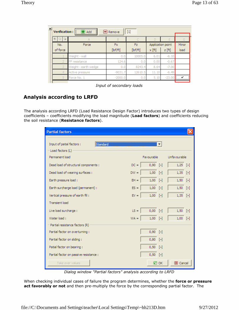
Input of secondary loads
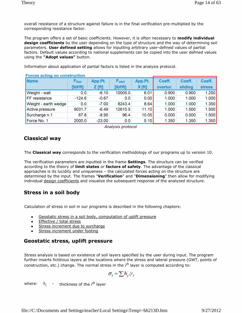
The analysis according LRFD (Load Resistance Design Factor) introduces two types of design coefficients – coefficients modifying the load magnitude (Load factors) and coefficients reducing the soil resistance (Resistance factors).
Dialog window "Partial factors" analysis according to LRFD
When checking individual cases of failure the program determines, whether the force or pressure act favorably or not and then pre-multiply the force by the corresponding partial factor. The
Analysis according to LRFD
Page 13 of 63Theory
9/27/2012file://C:\Documents and Settings\teacher\Local Settings\Temp\~hh213D.htm
overall resistance of a structure against failure is in the final verification pre-multiplied by the corresponding resistance factor.
The program offers a set of basic coefficients. However, it is often necessary to modify individual design coefficients by the user depending on the type of structure and the way of determining soil parameters. User defined setting allows for inputting arbitrary user-defined values of partial factors. Default values according to national supplements can be copied into the user defined values using the "Adopt values" button.
Information about application of partial factors is listed in the analysis protocol.
Analysis protocol
The Classical way corresponds to the verification methodology of our programs up to version 10.
The verification parameters are inputted in the frame Settings. The structure can be verified according to the theory of limit states or factors of safety. The advantage of the classical approaches is its lucidity and uniqueness – the calculated forces acting on the structure are determined by the input. The frames "Verification" and "Dimensioning" then allow for modifying individual design coefficients and visualize the subsequent response of the analyzed structure.
Calculation of stress in soil in our programs is described in the following chapters:
� Geostatic stress in a soil body, computation of uplift pressure � Effective / total stress � Stress increment due to surcharge � Stress increment under footing
Stress analysis is based on existence of soil layers specified by the user during input. The program further inserts fictitious layers at the locations where the stress and lateral pressure (GWT, points of
construction, etc.) change. The normal stress in the ith layer is computed according to:
Classical way
Stress in a soil body
Geostatic stress, uplift pressure
where: hi - thickness of the ith layer
Page 14 of 63Theory
9/27/2012file://C:\Documents and Settings\teacher\Local Settings\Temp\~hh213D.htm

If the layer is found below the ground water table, the unit weight of soil below the water table is specified with the help of inputted parameters of the soil as follows:
� for option "Standard" from expression:
Unit weight of water is assumed in the program equal to 10 kN/m3 or 0,00625 ksi.
Assuming inclined ground behind the structure (β ≠ 0) and layered subsoil the angle β, when
computingthe coefficient of earth pressure K, is reduced in the ith layer using the following expression:
Vertical normal stress σz is defined as:
γi - unit weight of soil
where: γsat - saturated unit weight of soil
γw - unit weight of water
- for option "Compute from porosity" from expression:
where: n - porosity
γs - specific weight of soil
γw - unit weight of water
where: V - volume of soil
Vp - volume of voids
Gd - weight of dry soil
where: γ - unit weight of the soil in the first layer under ground
γi - unit weight of the soil in the ith layer under ground
β - slope inclination behind the structure
Effective/total stress in soil
where: σz - vertical normal total stress
γef - submerged unit weight of soil
z - depth bellow the ground surface
Page 15 of 63Theory
9/27/2012file://C:\Documents and Settings\teacher\Local Settings\Temp\~hh213D.htm

This expression in its generalized form describes so called concept of effective stress:
Total, effective and neutral stress in the soil
Effective stress concept is valid only for the normal stress σ, since the shear stress τ is not
transferred by the water so that it is effective. The total stress is determined using the basic tools of theoretical mechanics, the effective stress is then determined as a difference between the total stress and neutral (pore) pressure (i.e. always by calculation, it can never be measured). Pore pressures are determined using laboratory or in-situ testing or by calculation. To decide whether to use the total or effective stresses is no simple. The following table may provide some general recommendations valid for majority of cases. We should realize that the total stress depends on the way the soil is loaded by its self weight and external effects. As for the pore pressure we assume that for flowing pore water the pore equals to hydrodynamic pressure and to hydrostatic pressure otherwise. For partial saturated soils with higher degree of it is necessary to account for the fact that the pore pressure evolves both in water and air bubbles.
In layered subsoil with different unit weight of soils in individual horizontal layers the vertical total stress is determined as a sum of weight of all layers above the investigated point and the pore pressure:
γw - unit weight of water
where: σ - total stress (overall)
σef - effective stress (active)
u - neutral stress (pore water pressure)
Assume conditions Drained layer Undrained layer
short – term effective stress total stress
long – term effective stress effective stress
where: σz - vertical normal total stress
γ - unit weight of soil
- unit weight of soil in natural state for soils above the GWT and dry layers
- unit weight of soil below water in other cases
Page 16 of 63Theory
9/27/2012file://C:\Documents and Settings\teacher\Local Settings\Temp\~hh213D.htm
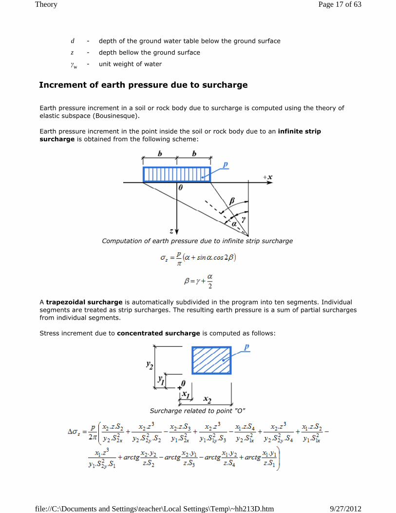
Earth pressure increment in a soil or rock body due to surcharge is computed using the theory of elastic subspace (Bousinesque).
Earth pressure increment in the point inside the soil or rock body due to an infinite strip surcharge is obtained from the following scheme:
Computation of earth pressure due to infinite strip surcharge
A trapezoidal surcharge is automatically subdivided in the program into ten segments. Individual segments are treated as strip surcharges. The resulting earth pressure is a sum of partial surcharges from individual segments.
Stress increment due to concentrated surcharge is computed as follows:
Surcharge related to point "O"
d - depth of the ground water table below the ground surface
z - depth bellow the ground surface
γw - unit weight of water
Increment of earth pressure due to surcharge
Page 17 of 63Theory
9/27/2012file://C:\Documents and Settings\teacher\Local Settings\Temp\~hh213D.htm
where:
Program system considers the following earth pressures categories:
� active earth pressure � passive earth pressure � earth pressure at rest
When computing earth pressures the program allows for distinguishing between the effective and total stress state and for establishing several ways of calculation of uplift pressure. In addition it is possible to account for the following effects having on the earth pressure magnitude:
� influence of loading � influence of water pressure � influence of broken terrain � friction between soil and back of structure � adhesion of soil � influence of earth wedge at cantilever jumps � influence of earthquake
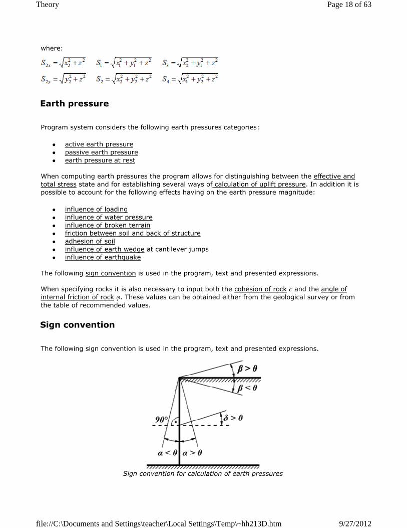
The following sign convention is used in the program, text and presented expressions.
When specifying rocks it is also necessary to input both the cohesion of rock c and the angle of internal friction of rock φ. These values can be obtained either from the geological survey or from the table of recommended values.
The following sign convention is used in the program, text and presented expressions.
Sign convention for calculation of earth pressures
Earth pressure
Sign convention
Page 18 of 63Theory
9/27/2012file://C:\Documents and Settings\teacher\Local Settings\Temp\~hh213D.htm
� inclination of the ground surface β is positive, when the ground rises upwards from the wall � inclination of the back of structure α is possitive, when the toe of the wall (at the back face)
is placed in the direction of the soil body when measured from the vertical line constructed from the upper point of the structure
� friction between the soil and back of structure δ is positive, if the resultant of earth pressure (thus also earth pressure) and normal to the back of structure form an angle measured in the clockwise direction
Active earth pressure is the smallest limiting lateral pressure developed at the onset of shear failure by wall moving away from the soil in the direction of the acting earth pressure (minimal wall rotation necessary for the evolution of active earth pressure is about 2 mrad, i.e. 2 mm/m ofthe wall height).
The following theories and approaches are implemented for the computation of active earth pressure assuming effective stress state:
� The Mazindrani theory � The Coulomb theory � The Müller-Breslau theory � The Caqouot theory � The Absi theory
For cohesive soils the tension cutoff condition is accepted, i.e. if due to cohesion the negative value of active earth pressure is developed or, according to more strict requirements, the value of "Minimal dimension pressure" is exceeded, the value of active earth pressure drops down to zero or set equal to the "Minimal dimensioning pressure".
The program also allows for running the analysis in total stresses.
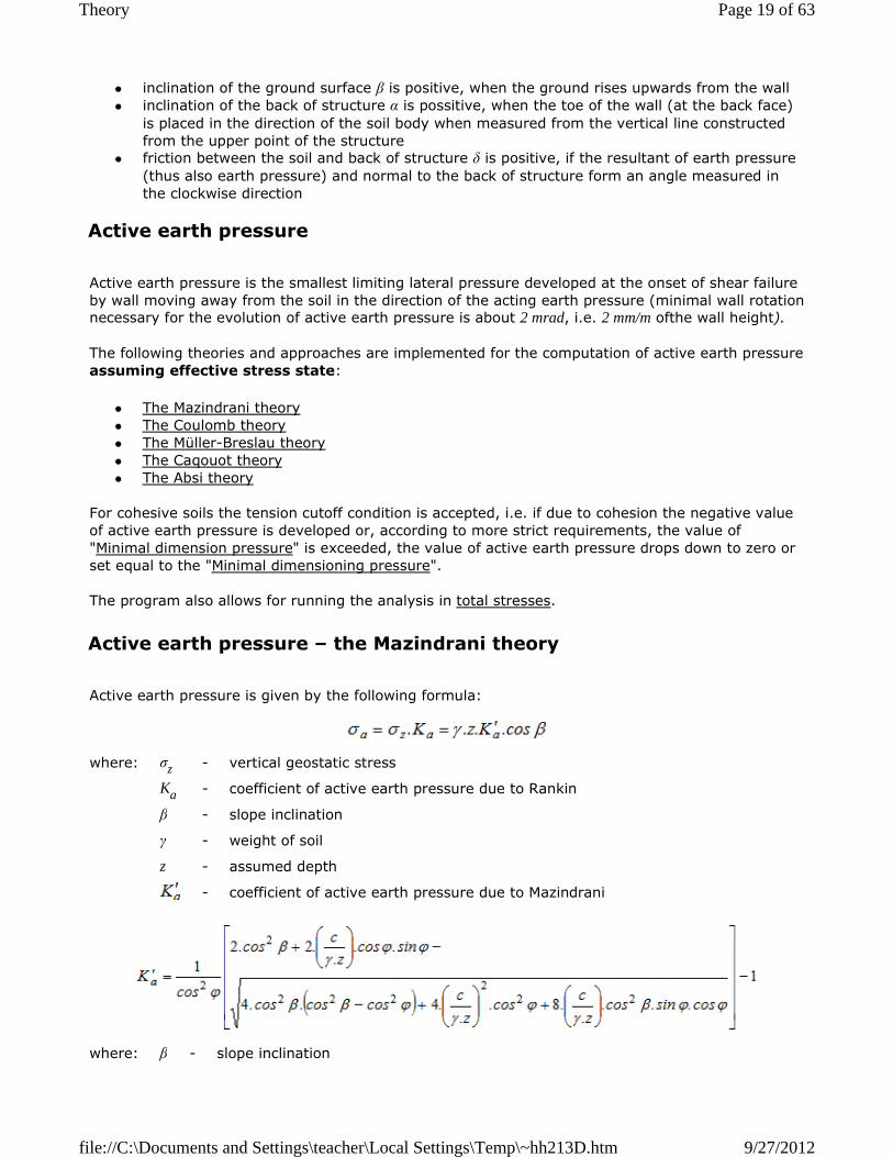
Active earth pressure is given by the following formula:
Active earth pressure
Active earth pressure – the Mazindrani theory
where: σz - vertical geostatic stress
Ka - coefficient of active earth pressure due to Rankin
β - slope inclination
γ - weight of soil
z - assumed depth
- coefficient of active earth pressure due to Mazindrani
where: β - slope inclination
Page 19 of 63Theory
9/27/2012file://C:\Documents and Settings\teacher\Local Settings\Temp\~hh213D.htm
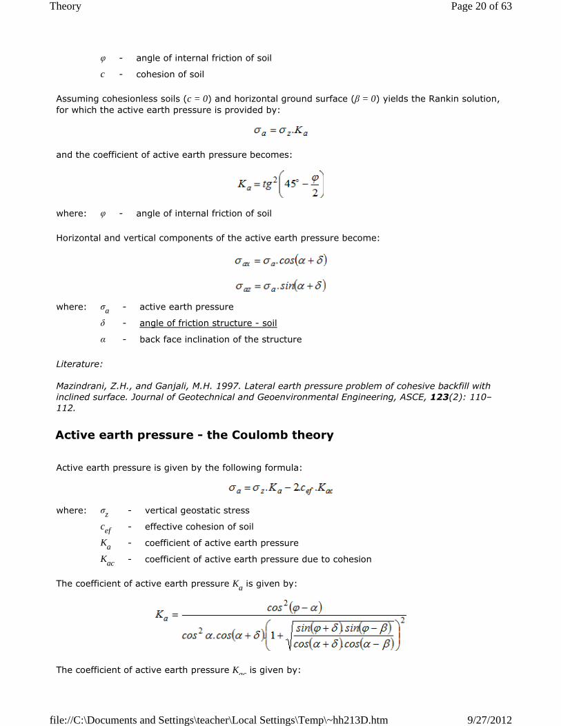
Assuming cohesionless soils (c = 0) and horizontal ground surface (β = 0) yields the Rankin solution, for which the active earth pressure is provided by:
and the coefficient of active earth pressure becomes:
Horizontal and vertical components of the active earth pressure become:
Literature:
Mazindrani, Z.H., and Ganjali, M.H. 1997. Lateral earth pressure problem of cohesive backfill with inclined surface. Journal of Geotechnical and Geoenvironmental Engineering, ASCE, 123(2): 110–112.
Active earth pressure is given by the following formula:
The coefficient of active earth pressure Ka is given by:
The coefficient of active earth pressure Kac is given by:
φ - angle of internal friction of soil
c - cohesion of soil
where: φ - angle of internal friction of soil
where: σa - active earth pressure
δ - angle of friction structure - soil
α - back face inclination of the structure
Active earth pressure - the Coulomb theory
where: σz - vertical geostatic stress
cef - effective cohesion of soil
Ka - coefficient of active earth pressure
Kac - coefficient of active earth pressure due to cohesion
Page 20 of 63Theory
9/27/2012file://C:\Documents and Settings\teacher\Local Settings\Temp\~hh213D.htm
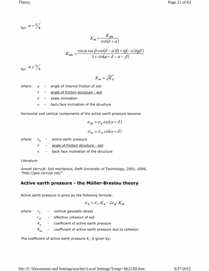
for:
for:
Horizontal and vertical components of the active earth pressure become:
Literature:
Arnold Verruijt: Soil mechanics, Delft University of Technology, 2001, 2006, "http://geo.verruijt.net/"
Active earth pressure is given by the following formula:
The coefficient of active earth pressure Ka is given by:
where: φ - angle of internal friction of soil
δ - angle of friction structure - soil
β - slope inclination
α - back face inclination of the structure
where: σa - active earth pressure
δ - angle of friction structure - soil
α - back face inclination of the structure
Active earth pressure - the Müller-Breslau theory
where: σz - vertical geostatic stress
cef - effective cohesion of soil
Ka - coefficient of active earth pressure
Kac - coefficient of active earth pressure due to cohesion
Page 21 of 63Theory
9/27/2012file://C:\Documents and Settings\teacher\Local Settings\Temp\~hh213D.htm
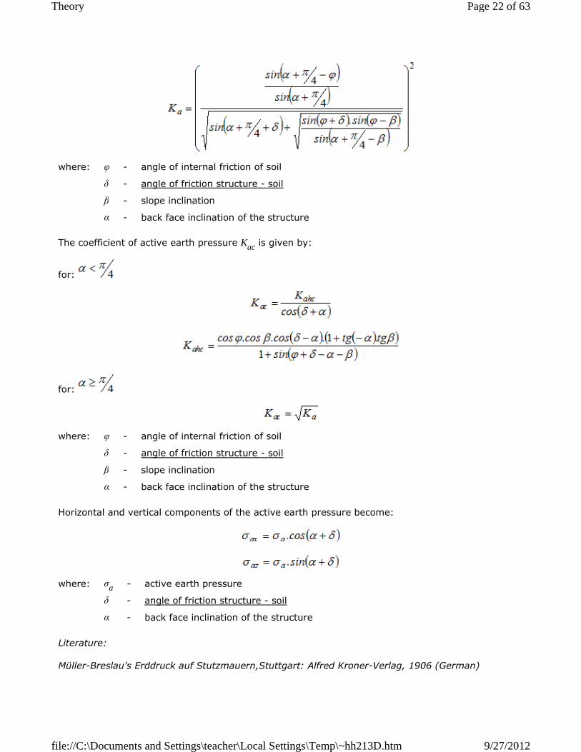
The coefficient of active earth pressure Kac is given by:
for:
for:
Horizontal and vertical components of the active earth pressure become:
Literature:
Müller-Breslau's Erddruck auf Stutzmauern,Stuttgart: Alfred Kroner-Verlag, 1906 (German)
where: φ - angle of internal friction of soil
δ - angle of friction structure - soil
β - slope inclination
α - back face inclination of the structure
where: φ - angle of internal friction of soil
δ - angle of friction structure - soil
β - slope inclination
α - back face inclination of the structure
where: σa - active earth pressure
δ - angle of friction structure - soil
α - back face inclination of the structure
Page 22 of 63Theory
9/27/2012file://C:\Documents and Settings\teacher\Local Settings\Temp\~hh213D.htm

Active earth pressure is given by the following formula:
The following analytical solution (Boussinesque, Caqouot) is implemented to compute the coefficient of active earth pressure Ka:
The coefficient of active earth pressure Kac is given by:
for:
Active earth pressure - the Caqouot theory
where: σz - vertical geostatic stress
cef - effective cohesion of soil
Ka - coefficient of active earth pressure
Kac - coefficient of active earth pressure due to cohesion
where: Ka - coefficient of active earth pressure due to Caquot
KaCoulomb - coefficient of active earth pressure due to Coulomb
ρ - conversion coefficient – see further
where: β - slope inclination behind the structure
φ - angle of internal friction of soil
δ - angle of friction structure - soil
Page 23 of 63Theory
9/27/2012file://C:\Documents and Settings\teacher\Local Settings\Temp\~hh213D.htm

for:
Horizontal and vertical components of the active earth pressure become:
Active earth pressure is given by the following formula:
The program takes values of the coefficient of active earth pressure Ka from a database, built upon
the values published in the book: Kérisel, Absi: Active and passive earth Pressure Tables, 3rd Ed. A.A. Balkema, 1990 ISBN 90 6191886 3.
The coefficient of active earth pressure Kac is given by:
for:
for:
where: φ - angle of internal friction of soil
δ - angle of friction structure - soil
β - slope inclination behind the structure
α - back face inclination of the structure
where: σa - active earth pressure
δ - angle of friction structure - soil
α - back face inclination of the structure
Active earth pressure - the Absi theory
where: σz - vertical geostatic stress
cef - effective cohesion of soil
Ka - coefficient of active earth pressure
Kac - coefficient of active earth pressure due to cohesion
Page 24 of 63Theory
9/27/2012file://C:\Documents and Settings\teacher\Local Settings\Temp\~hh213D.htm
Horizontal and vertical components of the active earth pressure become:
Literature:
Kérisel, Absi: Active and Passive Earth Pressure Tables, 3rd ed., Balkema, 1990 ISBN 90 6191886 3
When determining the active earth pressure in cohesive fully saturated soils, in which case the consolidation is usually prevented (undrained conditions), the horizontal normal total stress σx
receives the form:
The coefficient of earth pressure Kuc is given by:
Passive earth pressure is the highest limiting lateral pressure developed at the onset of shear failure
where: φ - angle of internal friction of soil
δ - angle of friction structure - soil
β - slope inclination
α - back face inclination of the structure
where: σa - active earth pressure
δ - angle of friction structure - soil
α - back face inclination of the structure
Active earth pressure – total stress
where: σx - horizontal total stress (normal)
σz - vertical normal total stress
Kuc - coefficient of earth pressure
cu - total cohesion of soil
where: Kuc - coefficient of earth pressure
cu - total cohesion of soil
au - total adhesion of soil to the structure
Passive earth pressure
Page 25 of 63Theory
9/27/2012file://C:\Documents and Settings\teacher\Local Settings\Temp\~hh213D.htm
by wall moving (penetrating) in the direction opposite to the direction of acting earth pressure (minimal wall rotation necessary for the evolution of passive earth pressure is about 10 mrad, i.e. 10 mm/m ofthe wall height). In most expressions used to compute the passive earth pressure the sign convention is assumed such that the usual values of δ corresponding to vertical direction of the friction resultant are negative. The program, however, assumes these values to be positive. A seldom variant with friction acting upwards is not considered in the program.
The following theories and approaches are implemented for the computation of passive earth pressure assuming effective stress state:
� The Rankin and Mazindrani theory � The Coulomb theory � The Caquot – Kérisel theory � The Müller – Breslau theory � The Absi theory � The Sokolovski theory
The program also allows for running the analysis in total stresses.
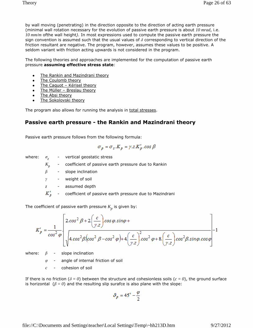
Passive earth pressure follows from the following formula:
The coefficient of passive earth pressure Kp is given by:
If there is no friction (δ = 0) between the structure and cohesionless soils (c = 0), the ground surface is horizontal (β = 0) and the resulting slip surafce is also plane with the slope:
Passive earth pressure - the Rankin and Mazindrani theory
where: σz - vertical geostatic stress
Kp - coefficient of passive earth pressure due to Rankin
β - slope inclination
γ - weight of soil
z - assumed depth
- coefficient of passive earth pressure due to Mazindrani
where: β - slope inclination
φ - angle of internal friction of soil
c - cohesion of soil
Page 26 of 63Theory
9/27/2012file://C:\Documents and Settings\teacher\Local Settings\Temp\~hh213D.htm

the Mazindrani theory then reduces to the Rankin theory. The coefficient of passive earth pressure is then provided by:
Passive earth pressure σp by Rankin for cohesionless soils is given:
Literature:
Arnold Verruijt: Soil mechanics, Delft University of Technology, 2001, 2006, http://geo.verruijt.net/
Mazindrani, Z.H., and Ganjali, M.H. 1997. Lateral earth pressure problem of cohesive backfill with inclined surface. Journal of Geotechnical and Geoenvironmental Engineering, ASCE, 123(2): 110–112.
Passive earth pressure follows from the following formula:
The coefficient of passive earth pressure Kp is given by:
The vertical σpv and horizontal σph components of passive earth pressure are given by:
where: φ - angle of internal friction of soil
where: γ - unit weight of soil
z - assumed depth
Kp - coefficient of passive earth pressure due to Rankin
Passive earth pressure - the Coulomb theory
where: σz - effective vertical geostatic stress
Kp - coefficient of passive earth pressure due to Coulomb
c - cohesion of soil
where: φ - angle of internal friction of soil
δ - angle of friction structure - soil
β - slope inclination
α - back face inclination of the structure
Page 27 of 63Theory
9/27/2012file://C:\Documents and Settings\teacher\Local Settings\Temp\~hh213D.htm
Literature:
Arnold Verruijt: Soil mechanics, Delft University of Technology, 2001, 2006, http://geo.verruijt.net/
Passive earth pressure follows from the following formula:
The vertical σpv and horizontal σph components of passive earth pressureare given by:
where: δ - angle of friction structure - soil
α - back face inclination of the structure
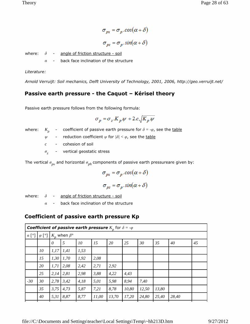
Passive earth pressure - the Caquot – Kérisel theory
where: Kp - coefficient of passive earth pressure for δ = -φ, see the table
ψ - reduction coefficient ψ for |δ| < φ, see the table
c - cohesion of soil
σz - vertical geostatic stress
where: δ - angle of friction structure - soil
α - back face inclination of the structure
Coefficient of passive earth pressure Kp
Coefficient of passive earth pressure Kp for δ = -φ
α [°] φ [°] Kp when β°
0 5 10 15 20 25 30 35 40 45
10 1,17 1,41 1,53
15 1,30 1,70 1,92 2,08
20 1,71 2,08 2,42 2,71 2,92
25 2,14 2,81 2,98 3,88 4,22 4,43
-30 30 2,78 3,42 4,18 5,01 5,98 8,94 7,40
35 3,75 4,73 5,87 7,21 8,78 10,80 12,50 13,80
40 5,31 8,87 8,77 11,00 13,70 17,20 24,80 25,40 28,40
Page 28 of 63Theory
9/27/2012file://C:\Documents and Settings\teacher\Local Settings\Temp\~hh213D.htm

45 8,05 10,70 14,20 18,40 23,80 90,60 38.90 49,10 60,70 69,10
10 1,36 1,58 1,70
15 1,68 1,97 2,20 2,38
20 2,13 2,52 2,92 3,22 3,51
25 2,78 3,34 3,99 4,80 5,29 5,57
-20 30 3,78 4,81 8,58 8,81 7,84 9,12 9,77
35 5,38 8,89 8,28 10,10 12,20 14,80 17,40 19,00
40 8,07 10,40 12,00 18,50 20,00 25,50 38,50 37,80 42,20
45 13,2 17,50 22,90 29,80 38,30 48,90 82,30 78,80 97,30 111,04
10 1,52 1,72 1,83 .
15 1,95 2,23 2,57 2,88
20 2,57 2,98 3,42 3,75 4,09
25 3,50 4,14 4,90 5,82 8,45 8,81
-10 30 4,98 8,01 7,19 8,51 10,10 11,70 12,80
35 7,47 9,24 11,30 13,80 18,70 20,10 23,70 2ó,00
40 12,0 15,40 19,40 24,10 29,80 37,10 53,20 55,10 61,80
45 21,2 27,90 38,50 47,20 80,80 77,30 908,20 124,00 153,00 178,00
10 1,84 1,81 1,93
15 2,19 2,46 2,73 2,91
20 3,01 3,44 3,91 4,42 4,66
25 4,28 5,02 5,81 8,72 7,71 8,16
0 30 8,42 7,69 9,19 10,80 12,70 14,80 15,90
35 10,2 12,60 15,30 18,80 22,30 28,90 31,70 34,90
40 17,5 22,30 28,00 34,80 42,90 53,30 78,40 79,10 88,70
45 33,5 44,10 57,40 74,10 94,70 120,00 153,00 174,00 240,00 275,00
10 1,73 1,87 1,98
15 2,40 2,65 2,93 3,12
20 3,45 3,90 4,40 4,96 5,23
10 25 5,17 5,99 6,90 7,95 9,11 9,67
30 8,17 9,69 11,40 13,50 15,90 18,50 19,90
35 13,8 16,90 20,50 24,80 29,80 35,80 42,30 46,60
40 25,5 32,20 40,40 49,90 61,70 76,40 110,00 113,00 127,00
45 52,9 69,40 90,90 116,00 148,00 i88,00 239,00 303,00 375,00 431,00
10 1,78 1,89 I 2,01
15 2,58 2,821 3,11 3,30
20 3,90 4,38 4,92 5,53 5,83
Page 29 of 63Theory
9/27/2012file://C:\Documents and Settings\teacher\Local Settings\Temp\~hh213D.htm

Reduction coefficient ψ for |δ| < φ
Passive earth pressure follows from the following formula:
The coefficient of passive earth pressure Kp is given by:
20 25 6,18 7,12 8,17 9,39 10,70 11,40
30 10,4 12,30 14,40 16,90 20,00 23,20 25,00
35 18,7 22,80 27,60 33,30 40,00 48,00 56,80 62,50
40 37,2 46,90 58,60 72,50 89,30 111,00 158,00 164,00 185,00
45 84,0 110,00 143,00 184,00 234,00 297,00 378,00 478,00 592,00 680,00
Reduction coefficient of passive earth pressure
φ[°] ψ for |δ| < φ
5 1,0 0,8 0,6 0,4 0,2 0,0
10 1,00 0,999 0,962 0,929 0,898 0,864
15 1,00 0,979 0,934 0,881 0,830 0,775
20 1,00 0,968 0,901 0,824 0,752 0,678
25 1,00 0,954 0,860 0,759 0,666 0,574
30 1,00 0,937 0,811 0,686 0,574 0,467
35 1,00 0,916 0,752 0,603 0,475 0,362
40 1,00 0,886 0,682 0,512 0,375 0,262
45 1,00 0,848 0,600 0,414 0,276 0,174
Passive earth pressure - the Müller – Breslau theory
where: Kp - coefficient of passive earth pressure
c - cohesion of soil
σz - vertical normal total stress
where: φ - angle of internal friction of soil
δ - angle of friction structure - soil
β - slope inclination
Page 30 of 63Theory
9/27/2012file://C:\Documents and Settings\teacher\Local Settings\Temp\~hh213D.htm
The vertical σpv and horizontal σph components of passive earth pressure are given by:
Literature:
Müller-Breslau's Erddruck auf Stutzmauern,Stuttgart: Alfred Kroner-Verlag, 1906 (German)
Passive earth pressure follows from the following formula:
The program takes values of the coefficient Kp from a database, built upon the tabulated values
published in the book: Kérisel, Absi: Active and passive earth Pressure Tables, 3rd Ed. A.A. Balkema, 1990 ISBN 90 6191886 3.
The vertical σpv and horizontal σph components of passive earth pressureare given by:
Literature:
Kérisel, Absi: Active and Passive Earth Pressure Tables, 3rd ed., Balkema, 1990 ISBN 90 6191886 3
Passive earth pressure follows from the following formula:
α - back face inclination of the structure
where: δ - angle of friction structure - soil
α - back face inclination of the structure
Passive earth pressure - the Absi theory
where: Kp - coefficient of passive earth pressure
c - cohesion of soil
σz - vertical normal total stress
where: δ - angle of friction structure - soil
α - back face inclination of the structure
Passive earth pressure - the Sokolovski theory
Page 31 of 63Theory
9/27/2012file://C:\Documents and Settings\teacher\Local Settings\Temp\~hh213D.htm

Individual expressions for determining the magnitude of passive earth pressure and slip surface are introduced in the sequel; the meaning of individual variables is evident from Fig.:
Passive eart pressure slip surface after Sokolovski
Angles describing the slip surface:
where: Kpg - passive earth pressure coefficient for cohesionless soils
Kpc - passive earth pressure coefficient due to cohesion
Kpp - passive earth pressure coefficient due to surcharge
σz - vertical normal total stress
where: φ - angle of internal friction of soil
δp - angle of friction structure - soil
β - slope inclination
Page 32 of 63Theory
9/27/2012file://C:\Documents and Settings\teacher\Local Settings\Temp\~hh213D.htm
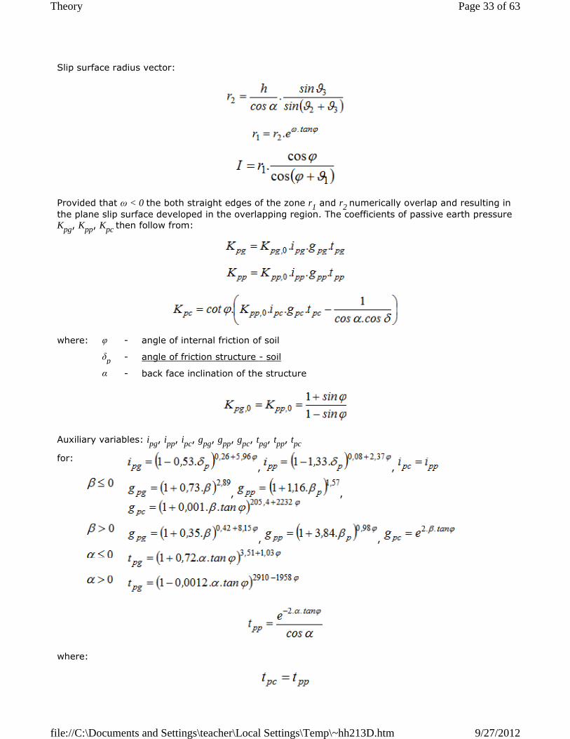
Slip surface radius vector:
Provided that ω < 0 the both straight edges of the zone r1 and r2 numerically overlap and resulting in the plane slip surface developed in the overlapping region. The coefficients of passive earth pressure Kpg, Kpp, Kpc then follow from:
Auxiliary variables: ipg, ipp, ipc, gpg, gpp, gpc, tpg, tpp, tpc
where:
where: φ - angle of internal friction of soil
δp - angle of friction structure - soil
α - back face inclination of the structure
for: , ,
, ,
, ,
Page 33 of 63Theory
9/27/2012file://C:\Documents and Settings\teacher\Local Settings\Temp\~hh213D.htm
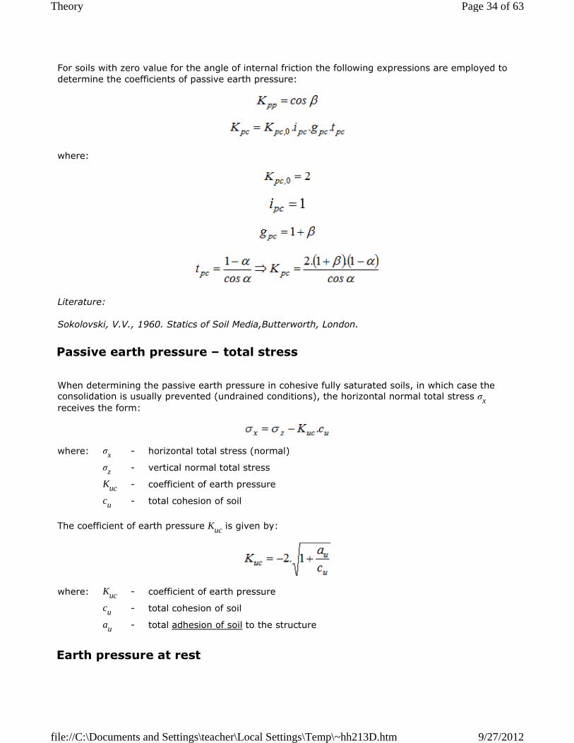
For soils with zero value for the angle of internal friction the following expressions are employed to determine the coefficients of passive earth pressure:
where:
Literature:
Sokolovski, V.V., 1960. Statics of Soil Media,Butterworth, London.
When determining the passive earth pressure in cohesive fully saturated soils, in which case the consolidation is usually prevented (undrained conditions), the horizontal normal total stress σx
receives the form:
The coefficient of earth pressure Kuc is given by:
Passive earth pressure – total stress
where: σx - horizontal total stress (normal)
σz - vertical normal total stress
Kuc - coefficient of earth pressure
cu - total cohesion of soil
where: Kuc - coefficient of earth pressure
cu - total cohesion of soil
au - total adhesion of soil to the structure
Earth pressure at rest
Page 34 of 63Theory
9/27/2012file://C:\Documents and Settings\teacher\Local Settings\Temp\~hh213D.htm

Earth pressure at rest rest is the horizontal pressure acting on the rigid structure. It is usually assumed in cases, when it is necessary to minimize the lateral and horizontal deformation of the sheeted soil (e.g. when laterally supporting a structure in the excavation pit up to depth below the current foundation or in general when casing soil with structures sensitive to non-uniform settlement), or when structures loaded by earth pressures are due to some technological reasons extremely rigid and do not allow for deformation in the direction of loading necessary to mobilize the active earth pressure.
Earth pressure at rest is given by:
For cohesive soils the Terzaghi formula for computing Kr is implemented in the program:
For cohesionless soils the Jáky expression is used:
When computing the pressure at rest for cohesive soils σr using the Jáky formula for the determination of coefficient of earth pressure at rest Kr, it is recommended to use the alternate angle of internal friction φn.
The way of computing the earth pressure at rest can be therefore influenced by the selection of the type of soil (cohesive, cohesionless) when inputting its parameters. Even typically cohesionless soil (sand, gravel) must be introduced as cohesive if we wish to compute the pressure at rest with the help of the Poisson ratio and vice versa.
For overconsolidated soils the expression proposed by Schmertmann to compute the coefficient of earth pressure at rest Kr is used:
The value of the coefficient of earth pressure at rest can be inputted also directly.
Influence of the inclined ground surface at the back of structure on earth pressure at rest is described here.
Literature:
Arnold Verruijt: Soil mechanics, Delft University of Technology, 2001, 2006, http://geo.verruijt.net/
where: ν - Poisson ratio
where: φ - angle of internal friction of soil
where: Kr - coefficient of earth pressure at rest
OCR - overconsolidation ratio
Earth pressure at rest for inclined ground surface at the back of structure
Page 35 of 63Theory
9/27/2012file://C:\Documents and Settings\teacher\Local Settings\Temp\~hh213D.htm

For inclined ground surface behind the structure (0° < β ≤ φ) the earth pressure at rest assumes the form:
For inclined back of wall the values of earth pressure at rest are derived from:
Normal and tangential components are given by:
The deviation angle from the normal line to the wall δ reads:
In some cases it appears more suitable for the analysis of earth pressures to introduce for cohesive soils an alternate angle of internal friction φn that also accounts for the influence of cohesive soil in
conjunction with the normal stress developed in the soil. The magnitude of the normal stress for determining the value of alternate angle of internal friction depends on the type of geotechnical problem, foundation conditions, etc. For deep seated foundation pits or constructions in homogeneous or relatively simple environment the normal stress is introduced in the centroid of the loading mass. In case of shallow pits or complex environment the normal stress is assumed in the
where: φ - angle of internal friction of soil
β - slope inclination
σz - vertical geostatic stress
Kr - coefficient of earth pressure at rest
where: α - back face inclination of the structure
σz - vertical geostatic stress
Kr - coefficient of earth pressure at rest
where: α - back face inclination of the structure
σz - vertical geostatic stress
Kr - coefficient of earth pressure at rest
where: α - back face inclination of the structure
Kr - coefficient of earth pressure at rest
Alternate angle of internal friction of soil
Page 36 of 63Theory
9/27/2012file://C:\Documents and Settings\teacher\Local Settings\Temp\~hh213D.htm

heel of the loading diagram – see figure:
Determination of normal stress for alternate angle of internal friction of soil φn
The alternate angle of internal friction of soil is given by:
When computing the pressure at rest for cohesive soils σr using the Jáky formula for the determination of coefficient of earth pressure at rest K0, it is recommended to use the alternate angle of internal friction φn.
Determination of alternate angle of internal friction of cohesive soil
Figures show the procedure of earth pressure analysis in the case of sloping terrain. The resulting shape of earth pressure distribution acting on the construction is obtained from the sum of triangular distributions developed by individual effects acting on the construction.
where: σz - vertical geostatic stress
φ - angle of internal friction of soil
c - cohesion of soil
Distribution of earth pressures in case of broken terrain
Page 37 of 63Theory
9/27/2012file://C:\Documents and Settings\teacher\Local Settings\Temp\~hh213D.htm
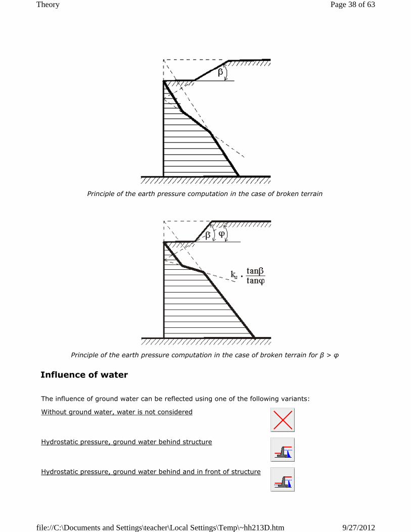
Principle of the earth pressure computation in the case of broken terrain
Principle of the earth pressure computation in the case of broken terrain for β > φ
The influence of ground water can be reflected using one of the following variants:
Influence of water
Without ground water, water is not considered
Hydrostatic pressure, ground water behind structure
Hydrostatic pressure, ground water behind and in front of structure
Page 38 of 63Theory
9/27/2012file://C:\Documents and Settings\teacher\Local Settings\Temp\~hh213D.htm

In this option the influence of ground water is not considered.
Complementary information:
If there are fine soils at and below the level of GWT, one should carefully assess an influence of full saturation in the region of capillary attraction. The capillary attraction is in the analysis reflected only by increased degree of saturation, and therefore the value of γsat is inserted into parameters of
soils.
To distinguish regions with different degree of saturation, one may insert several layers of the same soil with different unit weights. Negative pore pressures are not considered. However, for layers with different degree of saturation it is possible to use different values of shear resistance influenced by suction (difference in pore pressure of water and gas ua - uw).
The heel of a structure is sunk into impermeable subsoil so that the water flow below the structure is prevented. Water is found behind the back of structure only. There is no water acting on the front face. Such a case may occur when water in front of structure flow freely due to gravity or deep drainage is used. The back of structure is loaded by the hydrostatic pressure:
Hydrodynamic pressure
Special distribution of water pressure
Without ground water, water is not considered
Without ground water, water is not considered
Hydrostatic pressure, ground water behind structure
Hydrostatic pressure, ground water behind structure
where: γw - unit weight of water
hw - water tables difference
Page 39 of 63Theory
9/27/2012file://C:\Documents and Settings\teacher\Local Settings\Temp\~hh213D.htm
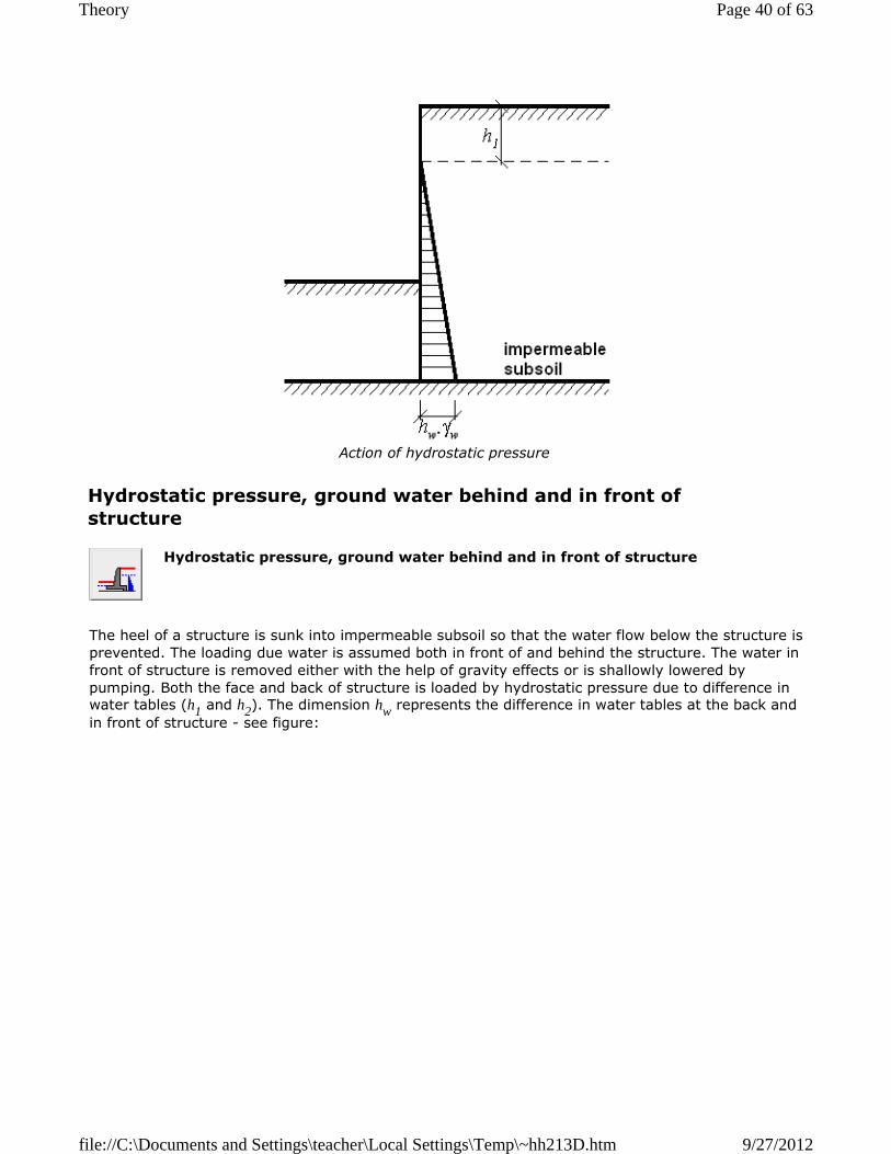
Action of hydrostatic pressure
The heel of a structure is sunk into impermeable subsoil so that the water flow below the structure is prevented. The loading due water is assumed both in front of and behind the structure. The water in front of structure is removed either with the help of gravity effects or is shallowly lowered by pumping. Both the face and back of structure is loaded by hydrostatic pressure due to difference in water tables (h1 and h2). The dimension hw represents the difference in water tables at the back and
in front of structure - see figure:
Hydrostatic pressure, ground water behind and in front of structure
Hydrostatic pressure, ground water behind and in front of structure
Page 40 of 63Theory
9/27/2012file://C:\Documents and Settings\teacher\Local Settings\Temp\~hh213D.htm

Action of hydrostatic pressure
The heel of a structure is sunk into permeable subsoil, which allows free water flow below the structure – see figure. The unit weight of soil lifted by uplift pressure γsu is modified to account for
flow pressure. These modifications then depend on the direction of water flow.
Action of hydrodynamic pressure
When computing the earth pressure in the area of descending flow the program introduces the
Hydrodynamic pressure
Hydrodynamic pressure
Page 41 of 63Theory
9/27/2012file://C:\Documents and Settings\teacher\Local Settings\Temp\~hh213D.htm
following value of the unit weight of soil:
and in the area of ascending flow the following value:
An average hydraulic slope is given:
If the change of unit weight of soil ∆γ provided by:
Is greater than the unit weight of saturated soil γsu, then the leaching appears in front of structure - as a consequence of water flow the soil behaves as weightless and thus cannot transmit any loading. The program then prompts a warning message and further assumes the value of γ = 0. The result therefore no longer corresponds to the original input – is safer.
This option allows an independent (manual) input of distribution of loading due to water at the back and in front of structure using ordinates of pore pressure at different depths. The variation of pressure between individual values is linear. At the same time it is necessary to input levels of tables of full saturation of a soil at the back h1 and in front h2 of structure including possible decrease of unit weight δy in front of structure due to water flow.
Example: Two separated horizon lines of ground water.
There are two permeable layers (sand or gravel) with one impermeable layer of clay in between, which causes separation of two hydraulic horizon lines – see figure:
where: γsu - unit weight of submerged soil
∆γ - alteration of unit weight of soil
i - an average seepage gradient
γw - unit weight of water
where: i - an average seepage gradient
hw - water tables difference
dd - seepage path downwards
du - seepage path upwards
where: i - an average seepage gradient
γw - unit weight of water
Special distribution of water pressure
Special distribution of water pressure
Page 42 of 63Theory
9/27/2012file://C:\Documents and Settings\teacher\Local Settings\Temp\~hh213D.htm

Example of pore pressure distribution
The variation of pore pressure above the clay layer is driven by free ground water table GWT1. The
distribution of pore pressure below the clay layer results from ratio in the lower separated ground water table GWT2, where the ground water is stressed. The pore pressure distribution in clay is
approximately linear.
The capillary attraction is in the analysis reflected only by increased degree of saturation, and therefore the value of γsat is inserted into parameters of soils.
To distinguish regions with different degree of saturation, one may insert several layers of the same soil with different unit weights. Negative pore pressures are not considered. However, for layers with different degree of saturation it is possible to introduce values of shear resistance influenced by suction.
The program makes it possible to account for the influence of tensile surface cracks filled with water. The analysis procedure is evident from the figure. The depth of tensile cracks is the only input parameter.
Influence of tensile cracks
Page 43 of 63Theory
9/27/2012file://C:\Documents and Settings\teacher\Local Settings\Temp\~hh213D.htm

Influence of tensile cracks
When determining the magnitude and distribution of earth pressures it is very difficult to qualify proportions of individual effects. This situation leads to uncertainty in the determination of earth pressure loading diagram. In reality we have to use in the design the most adverse distribution in favor of the safety of structure. For example, in case of braced structures in cohesive soils when using reasonable values of strength parameters of soil along the entire structure we may encounter tensile stresses in the upper part of the structure – see figure. Such tensile stresses, however, cannot be exerted on the sheeting structure (consequence of separation of soil due to technology of construction, isolation and drainage layer). In favor of the safe design of sheeting structure particularly in subsurface regions, where tensile stresses are developed during computation of the active earth pressure, the program offers the possibility to call the option "Minimal dimensioning pressure" in the analysis.
To determine the minimal dimensioning pressure the program employs for layers of cohesive soils as the minimal value of the coefficient of active earth pressure an alternate coefficient Ka = 0,2. Therefore it is ensured that the value of the computed active earth pressure will not drop below 20% of the vertical pressure (Ka ≥ 0,2) – see figure. Application of the minimal dimensioning pressure
assumes for example the possibility of increasing the lateral pressure due to filling of joint behind the sheeting structure with rain water. If the option of minimal dimensioning pressure is not selected the program simply assumes tension cutoff (Ka ≥ 0,0).
Minimal dimensioning pressure
Minimal dimensioning pressure
Page 44 of 63Theory
9/27/2012file://C:\Documents and Settings\teacher\Local Settings\Temp\~hh213D.htm
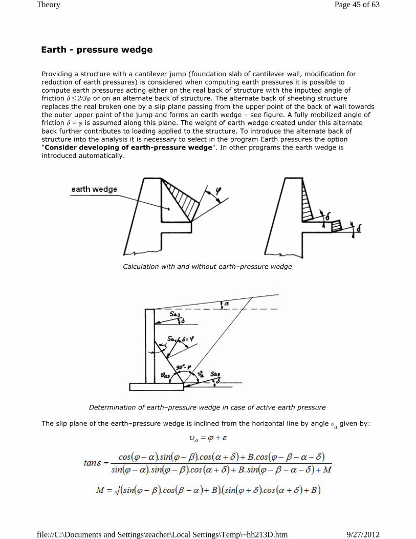
Providing a structure with a cantilever jump (foundation slab of cantilever wall, modification for reduction of earth pressures) is considered when computing earth pressures it is possible to compute earth pressures acting either on the real back of structure with the inputted angle of friction δ ≤ 2/3φ or on an alternate back of structure. The alternate back of sheeting structure replaces the real broken one by a slip plane passing from the upper point of the back of wall towards the outer upper point of the jump and forms an earth wedge – see figure. A fully mobilized angle of friction δ = φ is assumed along this plane. The weight of earth wedge created under this alternate back further contributes to loading applied to the structure. To introduce the alternate back of structure into the analysis it is necessary to select in the program Earth pressures the option "Consider developing of earth-pressure wedge". In other programs the earth wedge is introduced automatically.
Calculation with and without earth–pressure wedge
Determination of earth–pressure wedge in case of active earth pressure
The slip plane of the earth–pressure wedge is inclined from the horizontal line by angle υa given by:
Earth - pressure wedge
Page 45 of 63Theory
9/27/2012file://C:\Documents and Settings\teacher\Local Settings\Temp\~hh213D.htm
The shape of the earth wedge in the layered subsoil is determined such that for individual layers of soil above the wall foundation the program computes the angle υa, which then serves to determine the angle υas. Next, the program determines an intersection of the line drawn under the angle υas from the upper right point of the foundation block with the next layer. The procedure continues by drawing another line starting from the previously determined intersection and inclined by the angle υas. The procedure is terminated when the line intersects the terrain or wall surface, respectively. The wedge shape is further assumed in the form of triangle (intersection with wall) or rectangle (intersection with terrain).
The following types of surcharges are implemented in the program:
Active earth pressure
� Surface surcharge � Strip surcharge � Trapezoidal surcharge � Concentrated surcharge � Line surcharge
Earth pressure at rest
� Surface surcharge � Strip surcharge � Trapezoidal surcharge � Concentrated surcharge
Passive earth pressure
� Surface surcharge
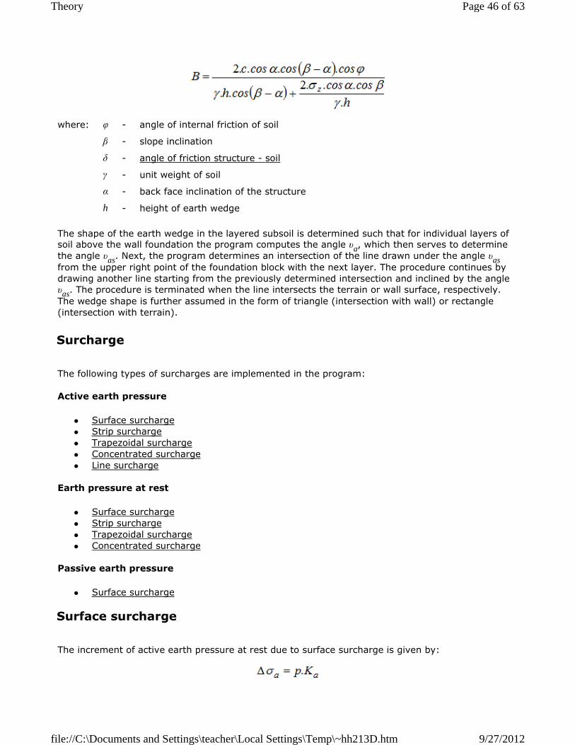
The increment of active earth pressure at rest due to surface surcharge is given by:
where: φ - angle of internal friction of soil
β - slope inclination
δ - angle of friction structure - soil
γ - unit weight of soil
α - back face inclination of the structure
h - height of earth wedge
Surcharge
Surface surcharge
Page 46 of 63Theory
9/27/2012file://C:\Documents and Settings\teacher\Local Settings\Temp\~hh213D.htm
The vertical uniform loading p applied to the ground surface induces therefore over the entire height of the structure a constant increment of active earth pressure – see figure:
Increment of active earth pressure due to vertical uniform ground surface surcharge
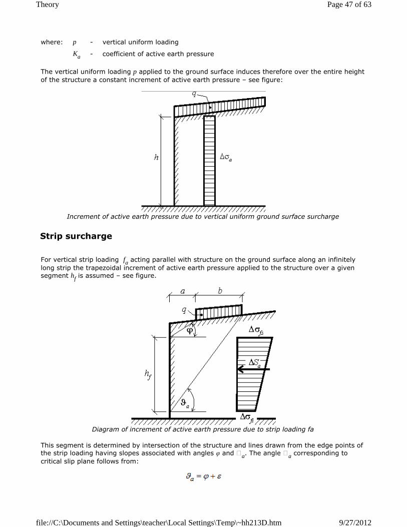
For vertical strip loading fa acting parallel with structure on the ground surface along an infinitely
long strip the trapezoidal increment of active earth pressure applied to the structure over a given segment hf is assumed – see figure.
Diagram of increment of active earth pressure due to strip loading fa
This segment is determined by intersection of the structure and lines drawn from the edge points of the strip loading having slopes associated with angles φ and ϑa. The angle ϑa corresponding to
critical slip plane follows from:
where: p - vertical uniform loading
Ka - coefficient of active earth pressure
Strip surcharge
Page 47 of 63Theory
9/27/2012file://C:\Documents and Settings\teacher\Local Settings\Temp\~hh213D.htm
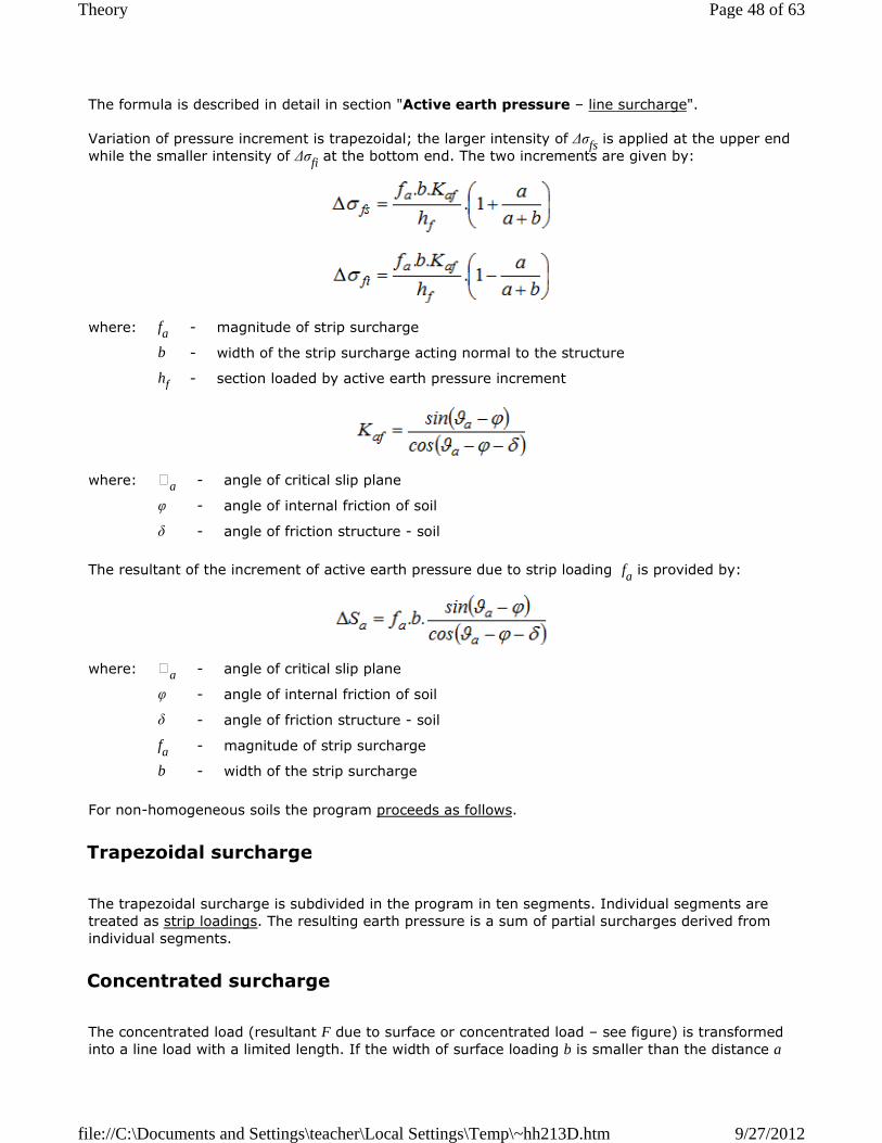
The formula is described in detail in section "Active earth pressure – line surcharge".
Variation of pressure increment is trapezoidal; the larger intensity of ∆σfs is applied at the upper end while the smaller intensity of ∆σfi at the bottom end. The two increments are given by:
The resultant of the increment of active earth pressure due to strip loading fa is provided by:
For non-homogeneous soils the program proceeds as follows.
The trapezoidal surcharge is subdivided in the program in ten segments. Individual segments are treated as strip loadings. The resulting earth pressure is a sum of partial surcharges derived from individual segments.
The concentrated load (resultant F due to surface or concentrated load – see figure) is transformed into a line load with a limited length. If the width of surface loading b is smaller than the distance a
where: fa - magnitude of strip surcharge
b - width of the strip surcharge acting normal to the structure
hf - section loaded by active earth pressure increment
where: ϑa - angle of critical slip plane
φ - angle of internal friction of soil
δ - angle of friction structure - soil
where: ϑa - angle of critical slip plane
φ - angle of internal friction of soil
δ - angle of friction structure - soil
fa - magnitude of strip surcharge
b - width of the strip surcharge
Trapezoidal surcharge
Concentrated surcharge
Page 48 of 63Theory
9/27/2012file://C:\Documents and Settings\teacher\Local Settings\Temp\~hh213D.htm

from the back of wall (see figure) the alternate line loading f having length 1+2*(a+b) receives the
form:
If the width b of surface loading is greater than the distance a from the back of wall (see figure) the alternate line loading f having length 1+2.(a+b) and width (a+b) reads:
Alternate loading for calculation of increment of active earth pressure
For non-homogeneous soils the program proceeds as follows.
Vertical infinitely long line loading f acting on the ground surface parallel with structure leads to a triangular increment of active earth pressure applied to the structure over a given segment hf – see
figure:
where: F - resultant due to surface or concentrated load
a - distance of loading from the back of wall
l - length of load
b - width of surface loading
where: F - resultant due to surface or concentrated load
a - distance of loading from the back of wall
l - length of load
b - width of surface loading
Line surcharge
Page 49 of 63Theory
9/27/2012file://C:\Documents and Settings\teacher\Local Settings\Temp\~hh213D.htm
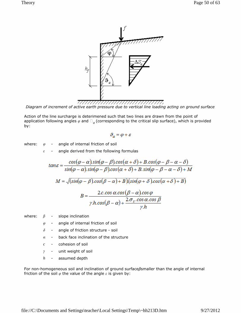
Diagram of increment of active earth pressure due to vertical line loading acting on ground surface
Action of the line surcharge is deterimened such that two lines are drawn from the point of application following angles φ and ϑa
(corresponding to the critical slip surface), which is provided
by:
For non-homogeneous soil and inclination of ground surfaceβsmaller than the angle of internal friction of the soil φ the value of the angle ε is given by:
where: φ - angle of internal friction of soil
ε - angle derived from the following formulas
where: β - slope inclination
φ - angle of internal friction of soil
δ - angle of friction structure - soil
α - back face inclination of the structure
c - cohesion of soil
γ - unit weight of soil
h - assumed depth
Page 50 of 63Theory
9/27/2012file://C:\Documents and Settings\teacher\Local Settings\Temp\~hh213D.htm

The resultant of the increment of active earth pressure due to line loading f is provided by:
For non-homogeneous soils the program proceeds as follows.
For non-homogeneous soil we proceed as follows:
� Compute the angle ϑa for a given soil layer.
� Determine the corresponding magnitude of force Sa and size of the corresponding pressure
diagram. � Determine the magnitude of earth pressure acting below the bottom edge of a given layer,
and its ratio with respect to the overall pressure magnitude. � The surcharge is reduced using the above ratio, then the location of this surcharge on the
upper edge of the subsequent layer is determined. � Compute again the angle ϑa for the next layer and repeat the previous steps until the
bottom of a structure is reached or the surcharge is completely exhausted.
An increment of uniformly distributed earth pressure at rest ∆σr caused by the vertical surface
loading applied on the ground surface behind the structure is computed using the following formula:
where: β - slope inclination
φ - angle of internal friction of soil
δ - angle of friction structure - soil
α - back face inclination of the structure
where: ϑa - angle of critical slip plane
φ - angle of internal friction of soil
δ - angle of friction structure - soil
f - magnitude of line surcharge
Surcharge in non-homogeneous soil
Surface surcharge
where: f - magnitude of surface surcharge
Kr - coefficient of earth pressure at rest
Page 51 of 63Theory
9/27/2012file://C:\Documents and Settings\teacher\Local Settings\Temp\~hh213D.htm

Diagram of increment of earth pressure at rest due to vertical uniform loading acting on ground surface
Uniform strip loading fa acting on the ground surface behind the structure parallel with vertical structure (see figure) creates an increment of earth pressure at rest ∆σr having the magnitude given
by:
Increment of earth pressure due to vertical strip surcharge
The trapezoidal surcharge is subdivided in the program in five segments. Individual segments are
Strip surcharge
where: fa - vertical strip surcharge
α, α1, α2 - evident from figure
Trapezoidal surcharge
Page 52 of 63Theory
9/27/2012file://C:\Documents and Settings\teacher\Local Settings\Temp\~hh213D.htm
treated as strip loadings. The resulting earth pressure is a sum of partial surcharges derived from individual segments.
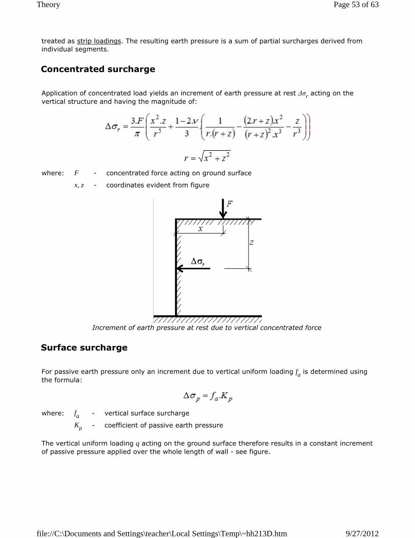
Application of concentrated load yields an increment of earth pressure at rest ∆σr acting on the
vertical structure and having the magnitude of:
Increment of earth pressure at rest due to vertical concentrated force
For passive earth pressure only an increment due to vertical uniform loading fa is determined using
the formula:
The vertical uniform loading q acting on the ground surface therefore results in a constant increment of passive pressure applied over the whole length of wall - see figure.
Concentrated surcharge
where: F - concentrated force acting on ground surface
x, z - coordinates evident from figure
Surface surcharge
where: fa - vertical surface surcharge
Kp - coefficient of passive earth pressure
Page 53 of 63Theory
9/27/2012file://C:\Documents and Settings\teacher\Local Settings\Temp\~hh213D.htm
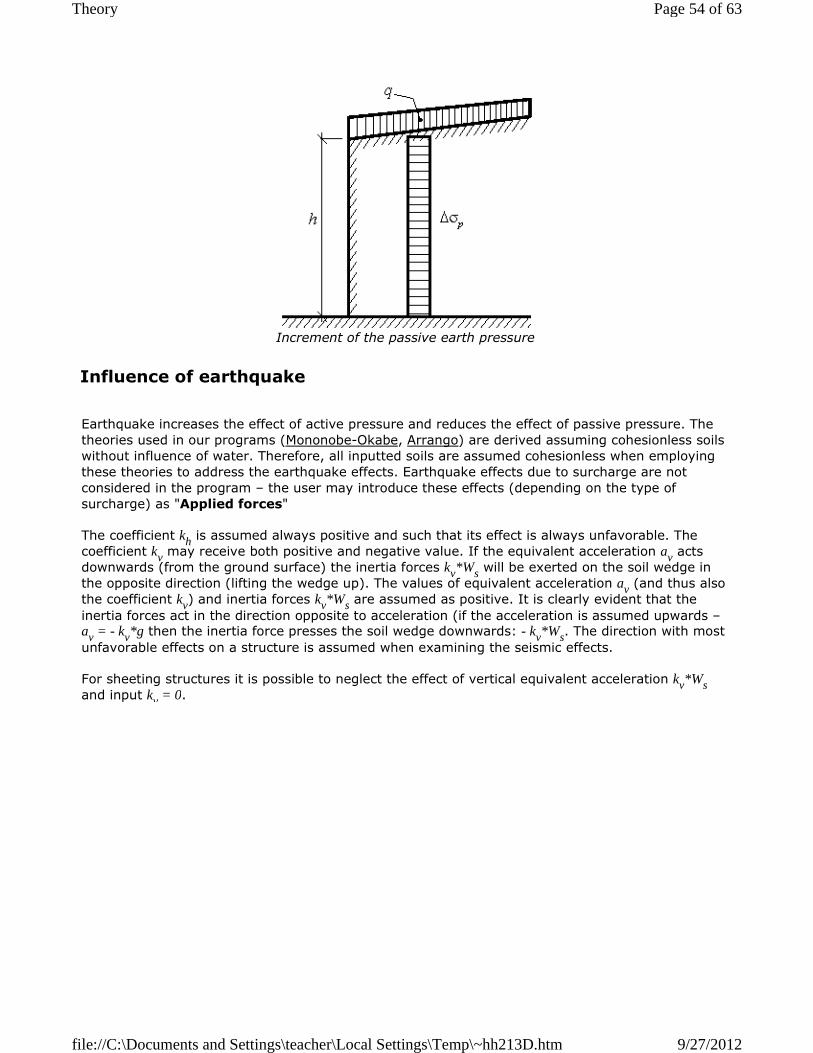
Increment of the passive earth pressure
Earthquake increases the effect of active pressure and reduces the effect of passive pressure. The theories used in our programs (Mononobe-Okabe, Arrango) are derived assuming cohesionless soils without influence of water. Therefore, all inputted soils are assumed cohesionless when employing these theories to address the earthquake effects. Earthquake effects due to surcharge are not considered in the program – the user may introduce these effects (depending on the type of surcharge) as "Applied forces"
The coefficient kh is assumed always positive and such that its effect is always unfavorable. The coefficient kv may receive both positive and negative value. If the equivalent acceleration av acts downwards (from the ground surface) the inertia forces kv*Ws will be exerted on the soil wedge in the opposite direction (lifting the wedge up). The values of equivalent acceleration av (and thus also the coefficient kv) and inertia forces kv*Ws are assumed as positive. It is clearly evident that the
inertia forces act in the direction opposite to acceleration (if the acceleration is assumed upwards –av = - kv*g then the inertia force presses the soil wedge downwards: - kv*Ws. The direction with most
unfavorable effects on a structure is assumed when examining the seismic effects.
For sheeting structures it is possible to neglect the effect of vertical equivalent acceleration kv*Ws and input kv = 0.
Influence of earthquake
Page 54 of 63Theory
9/27/2012file://C:\Documents and Settings\teacher\Local Settings\Temp\~hh213D.htm
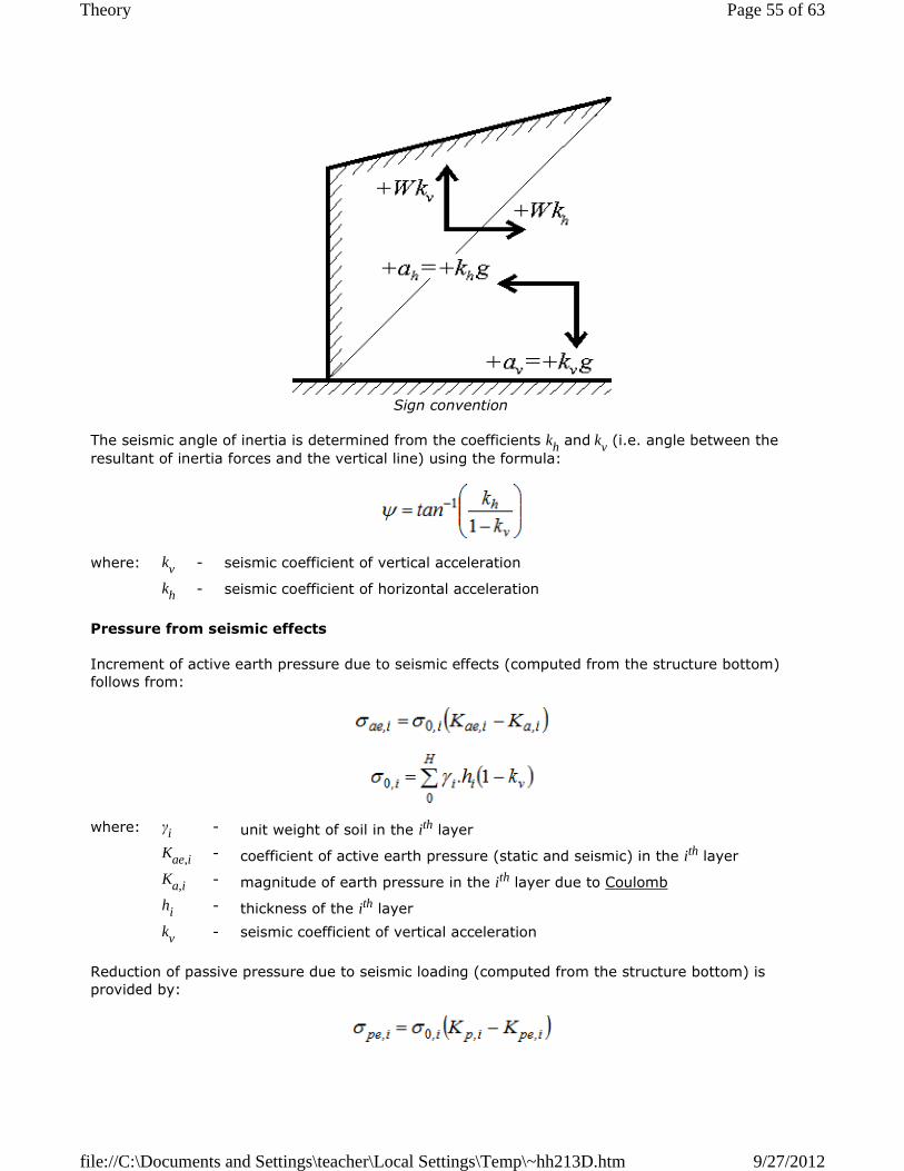
Sign convention
The seismic angle of inertia is determined from the coefficients kh and kv (i.e. angle between the
resultant of inertia forces and the vertical line) using the formula:
Pressure from seismic effects
Increment of active earth pressure due to seismic effects (computed from the structure bottom) follows from:
Reduction of passive pressure due to seismic loading (computed from the structure bottom) is provided by:
where: kv - seismic coefficient of vertical acceleration
kh - seismic coefficient of horizontal acceleration
where: γi - unit weight of soil in the ith layer
Kae,i - coefficient of active earth pressure (static and seismic) in the ith layer
Ka,i - magnitude of earth pressure in the ith layer due to Coulomb
hi - thickness of the ith layer
kv - seismic coefficient of vertical acceleration
Page 55 of 63Theory
9/27/2012file://C:\Documents and Settings\teacher\Local Settings\Temp\~hh213D.htm

Active earth pressure coefficients Kae,i and Kpe,iare computed using the Mononobe-Okabe theory or
the Arrango theory. If there is ground water in the soil body the program takes that into account.
The basic assumption in the program when computing earthquake is a flat ground surface behind structure with inclination β. If that is not the case the program approximates the shape of terrain by
a flat surface as evident from figure:
Terrain shape approximation
Point of application of resultant force
The resultant force is automatically positioned by the program into the center of the stress diagram. Various theories recommend, however, different locations of the resultant force – owing to that it is possible to select the point of application of the resultant force in the range of 0,33 - 0,7H (H is the structure height). Recommended (implicit) value is 0,66H. Having the resultant force the program determines the trapezoidal shape of stress keeping both the inputted point of application of the resultant force and its magnitude.
The coefficient Kae for active earth pressure is given by:
where: γi - unit weight of soil in the ith layer
Kpe,i - coefficient of active earth pressure (static and seismic) in the ith layer
Kp,i - magnitude of earth pressure in the ith layer due to Coulomb
hi - thickness of the ith layer
kv - seismic coefficient of vertical acceleration
Mononobe–Okabe theory
Page 56 of 63Theory
9/27/2012file://C:\Documents and Settings\teacher\Local Settings\Temp\~hh213D.htm

The coefficient Kpe for passive earth pressure is given by:
Deviation of seismic forces ψ must be for active earth pressure always less or equal to the difference of the angle of internal friction and the ground surface inclination (i.e. φ - β). If the values ψ of is greater the program assumes the value ψ = φ - β. In case of passive earth pressure the value of deviation of seismic forces ψ must be always less or equal to the sum of the angle of internal friction and the ground surface inclination (i.e. φ + β). The values of computed and modified angle ψ can be visualized in the output – in latter case the word MODIFIED is also displayed.
Example of the program output
Literature:
Mononobe N, Matsuo H 1929, On the determination of earth pressure during earthquakes. In Proc. Of the World Engineering Conf., Vol. 9, str. 176
Okabe S., 1926 General theory of earth pressure. Journal of the Japanese Society of Civil Engineers, Tokyo, Japan 12 (1)
The program follows the Coulomb theory to compute the values of Ka and Kp while taking into
account the dynamic values (α*, β*).
For active earth pressure:
where: γ - unit weight of soil
H - height of the structure
φ - angle of internal friction of soil
δ - angle of friction structure - soil
α - back face inclination of the structure
β - slope inclination
kv - seismic coefficient of vertical acceleration
kh - seismic coefficient of horizontal acceleration
ψ - seismic inertia angle
Arrango theory
Page 57 of 63Theory
9/27/2012file://C:\Documents and Settings\teacher\Local Settings\Temp\~hh213D.htm
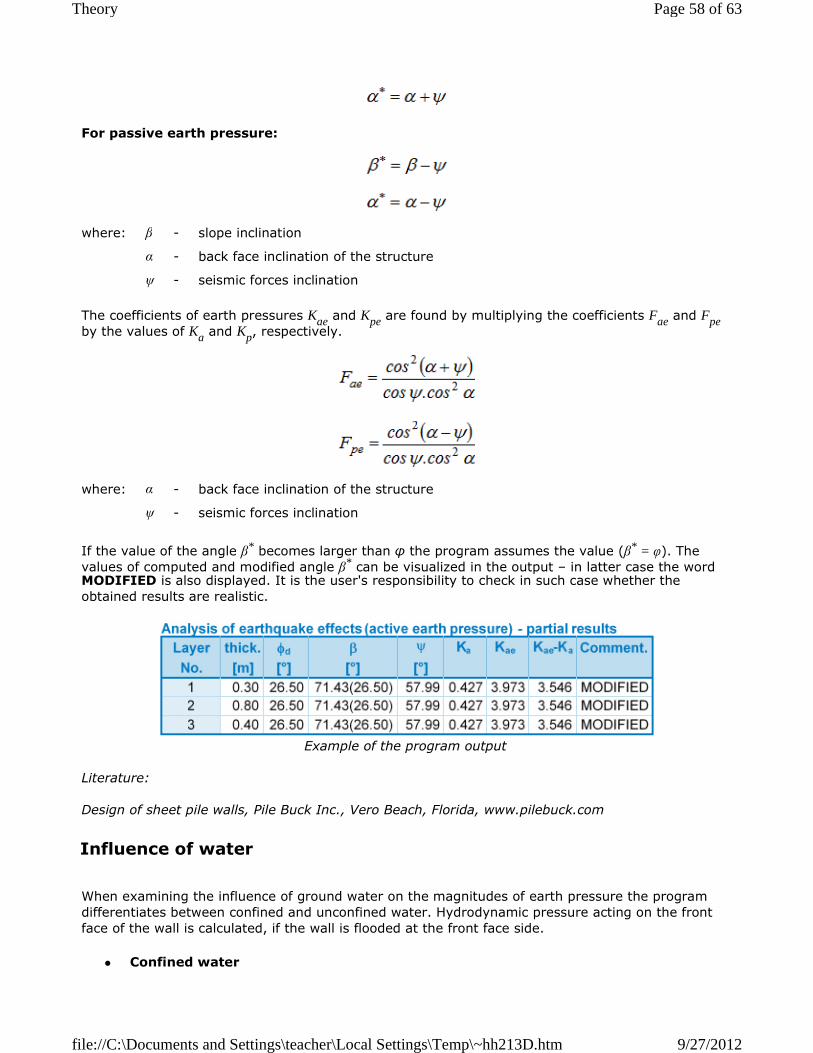
For passive earth pressure:
The coefficients of earth pressures Kae and Kpe are found by multiplying the coefficients Fae and Fpe by the values of Ka and Kp, respectively.
If the value of the angle β* becomes larger than φ the program assumes the value (β* = φ). The values of computed and modified angle β* can be visualized in the output – in latter case the word MODIFIED is also displayed. It is the user's responsibility to check in such case whether the obtained results are realistic.
Example of the program output
Literature:
Design of sheet pile walls, Pile Buck Inc., Vero Beach, Florida, www.pilebuck.com
When examining the influence of ground water on the magnitudes of earth pressure the program differentiates between confined and unconfined water. Hydrodynamic pressure acting on the front face of the wall is calculated, if the wall is flooded at the front face side.
� Confined water
where: β - slope inclination
α - back face inclination of the structure
ψ - seismic forces inclination
where: α - back face inclination of the structure
ψ - seismic forces inclination
Influence of water
Page 58 of 63Theory
9/27/2012file://C:\Documents and Settings\teacher\Local Settings\Temp\~hh213D.htm
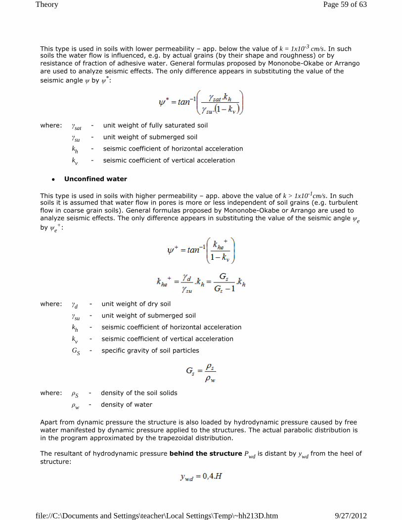
This type is used in soils with lower permeability – app. below the value of k = 1x10⁻³ cm/s. In such soils the water flow is influenced, e.g. by actual grains (by their shape and roughness) or by resistance of fraction of adhesive water. General formulas proposed by Mononobe-Okabe or Arrango are used to analyze seismic effects. The only difference appears in substituting the value of the
seismic angle ψ by ψ*:
� Unconfined water
This type is used in soils with higher permeability – app. above the value of k > 1x10⁻¹cm/s. In such soils it is assumed that water flow in pores is more or less independent of soil grains (e.g. turbulent flow in coarse grain soils). General formulas proposed by Mononobe-Okabe or Arrango are used to analyze seismic effects. The only difference appears in substituting the value of the seismic angle ψe
by ψe+:
Apart from dynamic pressure the structure is also loaded by hydrodynamic pressure caused by free water manifested by dynamic pressure applied to the structures. The actual parabolic distribution is in the program approximated by the trapezoidal distribution.
The resultant of hydrodynamic pressure behind the structure Pwd is distant by ywd from the heel of
structure:
where: γsat - unit weight of fully saturated soil
γsu - unit weight of submerged soil
kh - seismic coefficient of horizontal acceleration
kv - seismic coefficient of vertical acceleration
where: γd - unit weight of dry soil
γsu - unit weight of submerged soil
kh - seismic coefficient of horizontal acceleration
kv - seismic coefficient of vertical acceleration
GS - specific gravity of soil particles
where: ρS - density of the soil solids
ρw - density of water
Page 59 of 63Theory
9/27/2012file://C:\Documents and Settings\teacher\Local Settings\Temp\~hh213D.htm

and its magnitude follows from:
Hydrodynamic pressure acting on the front face of the wall
The resultant of hydrodynamic pressure on the front face of the wall Pwd is distant by ywd from
the heel of structure:
and its magnitude follows from:
If the coefficients kh and kv are not obtained from measurements it is necessary, providing the
analysis is carried out according to 1998-5 Eurocode 8: Design of structures for earthquake resistance - Part 5: Foundations, retaining structures and geotechnical aspects, to input these coefficients as follows:
where: H - height of the structure
where: γw - unit weight of water
kh - seismic coefficient of horizontal acceleration
H - height of the structure
where: H - height of the structure
where: γw - unit weight of water
kh - seismic coefficient of horizontal acceleration
H - height of the structure
EN 1998-5 Seismic effects
where: α - ratio of the design ground acceleration on type A ground (ag / g)
S - soil factor defined in EN 1998-1:2004, chapter 3.2.2.2
R - factor for the calculation of the horizontal seismic coefficient – see tab.
for:
for other cases:
Type of sheeting structure R
Free gravity walls that can accept a displacement up to (mm) 2
Page 60 of 63Theory
9/27/2012file://C:\Documents and Settings\teacher\Local Settings\Temp\~hh213D.htm
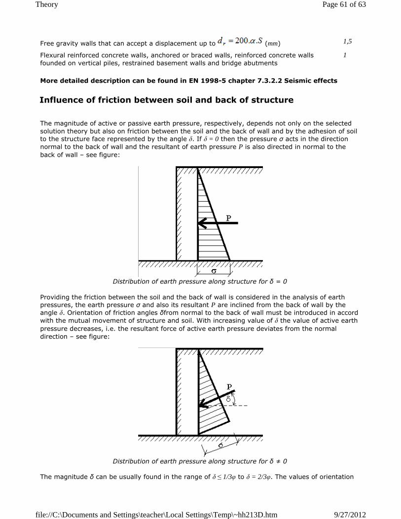
More detailed description can be found in EN 1998-5 chapter 7.3.2.2 Seismic effects
The magnitude of active or passive earth pressure, respectively, depends not only on the selected solution theory but also on friction between the soil and the back of wall and by the adhesion of soil to the structure face represented by the angle δ. If δ = 0 then the pressure σ acts in the direction normal to the back of wall and the resultant of earth pressure P is also directed in normal to the back of wall – see figure:
Distribution of earth pressure along structure for δ = 0
Providing the friction between the soil and the back of wall is considered in the analysis of earth pressures, the earth pressure σ and also its resultant P are inclined from the back of wall by the angle δ. Orientation of friction angles δfrom normal to the back of wall must be introduced in accord with the mutual movement of structure and soil. With increasing value of δ the value of active earth
pressure decreases, i.e. the resultant force of active earth pressure deviates from the normal direction – see figure:
Distribution of earth pressure along structure for δ ≠ 0
The magnitude δ can be usually found in the range of δ ≤ 1/3φ to δ = 2/3φ. The values of orientation
Free gravity walls that can accept a displacement up to (mm) 1,5
Flexural reinforced concrete walls, anchored or braced walls, reinforced concrete walls founded on vertical piles, restrained basement walls and bridge abutments
1
Influence of friction between soil and back of structure
Page 61 of 63Theory
9/27/2012file://C:\Documents and Settings\teacher\Local Settings\Temp\~hh213D.htm
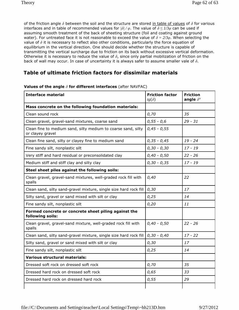
of the friction angle δ between the soil and the structure are stored in table of values of δ for various interfaces and in table of recommended values for |δ| / φ. The value of δ ≤ 1/3φ can be used if assuming smooth treatment of the back of sheeting structure (foil and coating against ground water). For untreated face it is not reasonable to exceed the value of δ = 2/3φ. When selecting the value of δ it is necessary to reflect also other conditions, particularly the force equation of equilibrium in the vertical direction. One should decide whether the structure is capable of transmitting the vertical surcharge due to friction on its back without excessive vertical deformation. Otherwise it is necessary to reduce the value of δ, since only partial mobilization of friction on the back of wall may occur. In case of uncertainty it is always safer to assume smaller vale of δ.
Values of the angle δ for different interfaces (after NAVFAC)
Table of ultimate friction factors for dissimilar materials
Interface material Friction factor tg(δ)
Friction angle δ°
Mass concrete on the following foundation materials:
Clean sound rock 0,70 35
Clean gravel, gravel-sand mixtures, coarse sand 0,55 - 0,6 29 - 31
Clean fine to medium sand, silty medium to coarse sand, silty or clayey gravel
0,45 - 0,55
Clean fine sand, silty or clayey fine to medium sand 0,35 - 0,45 19 - 24
Fine sandy silt, nonplastic silt 0,30 - 0,30 17 - 19
Very stiff and hard residual or preconsolidated clay 0,40 - 0,50 22 - 26
Medium stiff and stiff clay and silty clay 0,30 - 0,35 17 - 19
Steel sheet piles against the following soils:
Clean gravel, gravel-sand mixtures, well-graded rock fill with spalls
0,40 22
Clean sand, silty sand-gravel mixture, single size hard rock fill 0,30 17
Silty sand, gravel or sand mixed with silt or clay 0,25 14
Fine sandy silt, nonplastic silt 0,20 11
Formed concrete or concrete sheet piling against the following soils:
Clean gravel, gravel-sand mixture, well-graded rock fill with spalls
0,40 - 0,50 22 - 26
Clean sand, silty sand-gravel mixture, single size hard rock fill 0,30 - 0,40 17 - 22
Silty sand, gravel or sand mixed with silt or clay 0,30 17
Fine sandy silt, nonplastic silt 0,25 14
Various structural materials:
Dressed soft rock on dressed soft rock 0,70 35
Dressed hard rock on dressed soft rock 0,65 33
Dressed hard rock on dressed hard rock 0,55 29
Page 62 of 63Theory
9/27/2012file://C:\Documents and Settings\teacher\Local Settings\Temp\~hh213D.htm

When performing the analysis in the total stress state it is necessary not only to use the total shear strength parameters of soil φu , cu but also to know the adhesion a of soil to the structure face. The value of adhesion a is usually considered as a fraction of the soil cohesion c. The typical values of a for a given range of the cohesion c are listed in the following table.
Common values of the adhesion of soil a
Masonry on wood (Gross grain) 0,50 26
Steel on steel at sheet pile interlocks 0,30 17
Adhesion of soil
Soil Cohesion c [kPa] Adhesion a [kPa]
Soft and very soft cohesive soil 0 - 12 0 – 12
Cohesive soil with medium consistency 12 - 24 12 – 24
Stiff cohesive soil 24 - 48 24 - 36
Hard cohesive soil 48 - 96 36 – 46
Page 63 of 63Theory
9/27/2012file://C:\Documents and Settings\teacher\Local Settings\Temp\~hh213D.htm