Reliability Engineering 13 (1985) 175-180

There is No Such Thing as a Free Lunch: A Comment on a New Method for Reliability Demonstration

Benjamin Reiser

RAFAEL, PO Box 2250. Haifa 31021, Israel

(Received: 10 May 1985)

A B S T R A C T

A new distribution-free method for reliability demonstration tests has recently been proposed. It has further been claimed that this method can be applied when only one or two samples are available. An investigation of the confidence level properties of this method demonstrates that it is completely ineffective and that the claims made on its behalf are fallacious.

1 I N T R O D U C T I O N

Recently Ichikawa t has criticized the conventional method for distribution-free reliability demonstrat ion testing based on the binomial distribution for requiring the testing of a large number of samples. As an alternative he has suggested a new method based on certain probability inequalities which can be applied using only one or two samples.

The reliability demonstrat ion problem to be discussed can be formulated as follows: Let t be the random variable representing time to failure for some system with mean # and variance a 2. For some specified mission time t., it is required to verify that

Ps(t . , ) = Prob (t < t.,) < Psa (1)

where Pya is the maximum permitted probability of failure.

175 Reliability Engineering 0143-8174/85/$03.30 © Elsevier Applied Science Publishers Ltd, England, 1985. Printed in Great Britain

1 7 6 Benjamin Reiser

Ichikawa 1 demonstrated that eqn (1) is satisfied if

0 - 2

(# _ t,,)x + 0-~- < Ps . (2)

He further recommends that when n observations t l , . . . , t, are available on t, the usual estimates o f # and 0-2

~ /

IJ = i = y , ti/n i = 1

and

a x = ) , ( t i - / ~ ) 2 / ( n - 1)

i = l

be used in eqn (1) and that if the inequality is satisfied it be concluded that the reliability requirement is met. A sample of size n = 2 is sufficient to carry out these computa t ions . If the variance 0-2 is known, using /~ instead of/~ reduces eqn (2) to

X/1 -- P ~a O)

and a sample of size one can be used. Fur thermore , if it is known that the distr ibution of t is cont inuous with

one mode at the location of its mean then the sharper inequality

4a 2

9(~ - tin) 2 ~ e~" (4)

can be used instead of eqn (2). For known a : this reduces to

2a +

Thus, if for a given data set eqn (4) holds, Ichikawa concludes that the required reliability has been demonstra ted .

Ichikawa further suggests that the procedure using eqn (2) or (4) has a confidence level of about 50 %.

As Reiser z has noted, eqns (2) and (4) do not hold unless the following condit ion, overlooked by Ichikawa, 3 is added:

t~ ~ # (6)

A new method.[br reliability demonstration 177

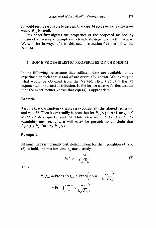
It would seem reasonable to assume that eqn (6) holds in many situations where Py~ is small.

This paper investigates the propert ies of the proposed method by means of a few simple examples which indicate its general ineffectiveness. We will, for brevity, refer to this new distribution-free method as the N D F M .

2 S O M E P R O B A B I L I S T I C P R O P E R T I E S OF T H E N D F M

In the following we assume that sufficient data are available to the experimenter such that # and a 2 are essentially known. We investigate what would be obtained f rom the N D F M when t actually has an exponential or normal distribution. In the former case we further assume that the experimenter knows that eqn (4) is appropriate.

Example 1

Assume that the r andom variable t is exponentially distr ibuted with/~ = 0 and o-2 = 0 2. Then it can readily be seen that for P I , < ½ there is no t,, > 0 which satisfies eqns (2) and (6). Thus, even without taking sampling variability into account , it will never be possible to conclude that Pi(t,,) < Py~ for any P ~ < ½.

Example 2

Assume that t is normally distributed. Then, for the inequalities (4) and (6) to hold, the mission time t,. must satisfy

2o-

3 _so /e (7)

Py(tm) = Prob (t < t,.) < Prob ( t _< #

( = Prob t - # < a 3

Thus

178 Be~!jamin Reiser

Since ( t - l ~ ) / t r has the standard normal distribution

- 3 (8)

where ~ represents the cumulative standard normal distribution function and t,~ is such that eqn (4) holds. Pj., is the maximum permitted failure

probability while ~N- 2/3x/Pz~) represents the maximum actual failure probability (assuming normality) given that eqn (4) is satisfied or, in other words, the maximum failure probability verifiable by the NDFM. Table 1 evaluates eqn (2) for various values of P~.

TABLE 1

~ - 2/3x/Py~)

Pfa 0.05 0.| 0.25 0.5

Py(t,,) < 0.001 4 0.001 7 0.091 2 0.17

From Table 1 we see that, for example, if Psa = 0.05 any case for which the actual failure probability is greater than 0.0014 but still less than 0.05 could never be identified as meeting the reliability criteria of Pya = 0.05 by means of the NDFM.

These two examples show the extreme conservativeness of the criteria (2) and (4). Many cases which, in fact, meet the reliability requirement could never (regardless of sample size) be demonstrated to do so by means of the NDFM.

3 SOME S A M P L I N G PROPERTIES OF THE NDFM

Assume that the experimenter has the observations ti, i = l , . . . , n available, that a 2 is known, and that Psa = 0.05 for some given t,,.

E x a m p l e 1

Assume that n = 1 and that the actual distribution is exponential with mean 0. The experimenter using the N D F M will conclude that the reliability requirement is met if (from eqn (3))

/J = t 1 >_ t,~ + 4.4a (9)

A new method.lbr reliability demonstration 179

If t,, is such that the reliability requirement is actually met, then

1 - e-tin/° < 0"05

or, equivalently, that

0 < t,, < - 0 In 0.95 = 0.050

Not ing that tr = 0 results in

0.011 = e - 4"'~5

= Prob(t~ >_ 4.450) < Prob (t 1 > t,, + 4-4tr) < Prob (t~ > 4.40)

= e - 4 ~ = 0.012

Thus, the probabili ty of concluding that the reliability requirement is met when it is in fact met is at most 0.012. One certainly cannot claim a 50 ~ confidence level here. As example 1 of Section 2 shows, increasing the sample size n does not help. As n increases the distribution of # becomes more concentra ted a round 0 = a and thus the probabili ty of eqn (9) being satisfied decreases.

Example 2

Assume that t is normally distr ibuted and that the experimenter while not knowing the distribution knows that it is cont inuous with one mode at the location of its mean and therefore applies eqn (5). Thus for n = 1 the N D F M states that the reliability requirement is demonst ra ted if

~ = t 1 ~ t,, + 3.0tr (10)

If t,, is such that the requirement of Pfa = 0.05 is met exactly, i.e. Py( t , , )=0 .05 , then t m = # - l ' 6 4 5 a and eqn (10) becomes t l > # + 1.355tr. Under the normal i ty assumpt ion

P r o b ( / l > # + l . 3 5 5 a ) = P r ° b ( t ~ - # > t r 1 . 355 )=0 .09

Thus, for P.r(t,,) = PIa = 0.05 there is a 9 ~ probabili ty of concluding that the requirement is met. This can be compared with the 50 ~ claimed for the N D F M .

Note that as n increases the Prob(~-># + 1.355a)decreases. The N D F M has the undesirable proper ty of performing worse with increasing sample size.

180 Ben/arnin Reiser

4 CO NCLUSIONS

The conventional (binomially based) nonparametric method for reliability demonstration has been criticized for requiring too large a sample size. However, this is simply the price that must be paid for not making parametric assumptions. The N D F M attempts to avoid paying this price through the use of certain inequalities. In fact the price is paid in a different manner. The N D F M provides an extremely conservative procedure for which in many cases products with very low (and sometimes even zero) failure probability will not be deemed acceptable. This property makes the N D F M completely ineffective.

A C K N O W L E D G E M E N T

I wish to thank Mrs Markiewicz for pointing out an error in an earlier draft of this paper.

REFERENCES

1. Ichikawa, M. Proposal of a new distribution-free method for reliability demonstration tests, Reliability Engineering, 9(2) (1984), pp. 99-105.

2. Reiser, B. A remark on Ichikawa's upper bound of probability of failure, this issue, pp. 181-3.

3. Ichikawa, M. New formula for upper bound of probability of failure, Reliability Engineering, 5(3) (1983), pp. 173-80.