thermal and thermal-mechanical analysis of thermo-active pile
TRANSCRIPT
Thermal and Thermal-Mechanical Analysis
of Thermo-Active Pile Foundations
Rui Manuel Freitas Assunção
Thesis to obtain the Master of Science Degree in
Civil Engineering
Supervisor: Prof. Peter John Bourne-Webb
Examination Committee
Chairperson: Prof. Jaime Alberto dos Santos
Supervisor: Prof. Peter John Bourne-Webb
Member of Committee: Prof. Teresa Maria Bodas de Araújo Freitas
March 2014

ii

iii
Abstract
Abstract
Thermo-active foundations make use of shallow geothermal energy to heat or cool buildings. By making
use of this green and renewable energy form, this technology can significantly reduce building energy
and maintenance costs in the long term and reduce carbon dioxide emissions. However, a complete
understanding of the thermal-mechanical behaviour of such foundations has not yet been achieved
which has been a major obstacle to the uptake and the industrial development of this technology. A
thermal and thermal-mechanical numerical study of a thermal active pile was performed in this thesis
using the finite element software Abaqus. The thermal analysis focused on some of the modelling
aspects of the problem such as the simulation of the heating of the pile and definition of the ground
surface temperature. The thermal-mechanical analysis studied the effect, in terms of thermally induced
stresses in the pile, of the relationship between soil and concrete coefficients of thermal expansion, of
the ground surface temperature and of the pile length to diameter ratio. The relationship between soil
and concrete coefficient of thermal expansion coefficients was found to have a key role in the observed
behaviour of the pile affecting both the direction (compression/tension) and the magnitude of the
developed thermally induced stresses in the pile. The ground surface temperature showed an important
effect when the soil was more thermally expansive than concrete, leading to considerable further stress
changes in the pile. An increase in the pile length to diameter ratio also led to an increase of the thermally
induced stresses in the pile.
Keywords
Foundation pile; thermal-mechanical; geothermal energy; finite elements.

iv
Resumo
v
Resumo
As fundações termoativas usam energia geotérmica superficial para aquecer e arrefecer edifícios.
Através do uso desta energia renovável e amiga do ambiente, esta tecnologia permite reduzir
significativamente os custos de aquecimento/arrefecimento de um edifício a longo prazo e as suas
emissões de dióxido de carbono. No entanto, um entendimento completo do comportamento
termomecânico destas fundações ainda não foi alcançado, o que tem sido um dos maiores obstáculos
ao desenvolvimento industrial desta tecnologia. Um estudo numérico térmico e termomecânico de uma
estaca termoativa foi realizado nesta tese através do uso do software de elementos finitos Abaqus. A
análise térmica focou-se em alguns aspetos de modelação do problema como a simulação do
aquecimento da estaca termoativa e a correta definição da temperatura da superfície do solo. A análise
termomecânica estudou o efeito, em termos de esforços induzidos termicamente na estaca, da relação
entre os coeficientes de expansão térmica do solo e do betão, da temperatura da superfície do solo e
da relação entre o diâmetro e o comprimento da estaca. Os resultados mostraram que a relação entre
o coeficiente de expansão térmica do solo e do betão desempenha um papel fundamental no
comportamento da estaca, afetando tanto a direção como a magnitude dos esforços termicamente
induzidos. Quando o solo tem maior coeficiente de expansão térmica que o betão, a temperatura da
superfície do solo exibiu um efeito importante na estaca, levando a consideráveis alterações de
esforços na mesma. Um aumento da relação comprimento/diâmetro da estaca conduziu a um aumento
dos esforços termicamente induzidos na mesma.
Palavras-chave
Estaca; termomecânica; energia geotérmica; elementos finitos.

vi

vii
Table of Contents
Table of Contents
Abstract ...................................................................................................................... iii
Resumo ...................................................................................................................... iv
Table of Contents ...................................................................................................... vii
List of Figures ............................................................................................................. ix
List of Tables ............................................................................................................. xii
List of Acronyms ....................................................................................................... xiii
List of Symbols ......................................................................................................... xiv
1 Introduction .................................................................................................... 1
1.1 Overview ........................................................................................................... 2
1.2 Motivation and Contents ................................................................................... 3
1.3 Structure of the Thesis ...................................................................................... 4
2 Geothermal Energy and Heat Pump Systems ............................................... 5
2.1 Shallow Geothermal Energy and its Use ........................................................... 6
2.2 Ground Source Heat Pump Systems ................................................................ 7
2.2.1 Introduction ............................................................................................................ 7
2.2.2 Efficiency of the GSHP Systems ........................................................................... 9
3 Heat Transfer Mechanisms .......................................................................... 11
3.1 Heat Transfer Mechanisms ..............................................................................12
3.1.1 Conduction ........................................................................................................... 12
3.1.2 Convection ........................................................................................................... 13
3.1.3 Radiation .............................................................................................................. 13
3.2 Heat Transfer in Soils ......................................................................................13
3.2.1 Thermal Conduction in Soils and Concrete ......................................................... 14
3.2.2 Thermal Expansion in Soils and Concrete .......................................................... 16
3.3 Heat Transfer in Thermo-Active Piles...............................................................17
4 The Effect of Heating and Cooling of a Pile ................................................. 19
4.1 Thermally Induced Deformation – General Principles ......................................20
4.1.1 Free Body Response (No Restraint) ................................................................... 20

viii
4.1.2 Perfectly Restrained Body ................................................................................... 21
4.1.3 Partially Restrained Body .................................................................................... 21
4.2 Experimental Observations of the Effect of Heating and Cooling a Pile............23
4.2.1 École Polytechnique Fédérale de Lausanne ....................................................... 23
4.2.2 Lambeth College, London ................................................................................... 27
4.3 Numerical Analysis of the Effect of Heating and Cooling a Pile ........................29
4.3.1 Bodas Freitas et al., 2013 and Cruz Silva, 2012 ................................................. 29
4.3.2 Di Donna et al., 2013 ........................................................................................... 31
4.3.3 Suryatriyastuti et al., 2013 ................................................................................... 34
5 Thermal Analysis ......................................................................................... 39
5.1 Introduction ......................................................................................................40
5.2 Thermal Load through the Pile .........................................................................40
5.2.1 Axisymmetric Thermal Model .............................................................................. 41
5.2.2 2D Thermal Model ............................................................................................... 47
5.3 Thermal Loss through the Ground-Floor Slab and Ground Surface Temperature 51
5.3.1 Numerical Model Implementation ........................................................................ 51
5.3.2 Analysis Methodologies and Objectives .............................................................. 53
5.3.3 Results and Discussion ....................................................................................... 53
6 Thermal-Mechanical Analyses ..................................................................... 57
6.1 Introduction ......................................................................................................58
6.2 Numerical Model Implementation .....................................................................58
6.2.1 Materials and material behaviour ........................................................................ 58
6.2.2 Geometry, Mesh, Boundary Conditions and Initial Conditions ............................ 59
6.2.3 Pile-Soil Interface Behaviour ............................................................................... 61
6.2.4 Model Validation .................................................................................................. 62
6.3 Analysis Methodology and Objectives ..............................................................64
6.4 Results and Discussion ....................................................................................66
6.4.1 Baseline Analysis................................................................................................. 66
6.4.2 Parameter Study .................................................................................................. 69
7 Conclusions ................................................................................................. 81
7.1 Conclusions and Results Summary .................................................................82
7.2 Future Developments .......................................................................................83
References ............................................................................................................... 85

ix
List of Figures
List of Figures Figure 1-1. Number of energy piles installed in Austria between 1984 and 2004 (Brandl, 2006). 2
Figure 2-1. Ground temperature at depth in Europe and tropics (Brandl, 2006). ......................... 6
Figure 2-2. Various types of ground heat exchangers (Amis, 2011). ............................................ 7
Figure 2-3. Scheme of a ground source heat pump system with energy piles as ground heat exchangers (Brandl, 2006). ................................................................................. 8
Figure 2-4. Heat pump and its interactions with the primary and secondary circuits (Bourne-Webb, 2014). ................................................................................................................... 8
Figure 3-1. Predominant heat transfer mechanisms by grain size and degree of saturation (Loveridge 2012, redrawn from Farouki, 1986). ................................................ 14
Figure 3-2. Soil thermal conductivity values as a function of moisture content (ASHRAE Fundamentals, 2009). ........................................................................................ 15
Figure 3-3. Thermal volumetric strain of Kaolin clay during drained heating (Cekerevac & Laloui (2004)). .............................................................................................................. 17
Figure 3-4. Thermo-active pile heat transfer: a) plan of thermal pile components; b) temperature differences (Powrie & Loveridge, 2013). ........................................................... 18
Figure 4-1. Thermal response of a non-restrained pile (free body): a) heating; b) cooling (Bourne-Webb, et al., 2013)............................................................................................. 20
Figure 4-2. Thermal response of a perfectly restrained pile: a) heating; b) cooling (Bourne-Webb, et al., 2013). ....................................................................................................... 21
Figure 4-3. Thermal response of a pile laterally restrained: (a) heating; (b) cooling (Bourne-Webb, et al., 2013). ....................................................................................................... 22
Figure 4-4. Thermal response of a pile laterally and end restrained: (a) heating; (b) cooling (Bourne-Webb, et al., 2013). ............................................................................. 22
Figure 4-5. Combined mechanical and thermal load effects on a partially restrained pile. Dash-dotted lines represent the effect of stronger thermal load or pile restraint. (a) Mechanical load only; (b) combined mechanical load and heating; (c) combined mechanical load and cooling; (Bourne-Webb, et al., 2013). .............................. 23
Figure 4-6. Soil stratigraphy and location of measurement instruments (Laloui et al., 2006). .... 24
Figure 4-7. Test pile configuration (Laloui et al., 2006). .............................................................. 24
Figure 4-8. Thermo-mechanical loading history (Laloui et al., 2006). ......................................... 25
Figure 4-9. Temperature values imposed in the pile (Laloui et al., 2006). .................................. 26
Figure 4-10. Thermal vertical stresses under a thermal load of 13.4ºC (Laloui et al., 2006). ..... 26
Figure 4-11. Thermo-mechanical vertical stresses in the pile: (a) experimental results; (b) numerical simulations). ...................................................................................... 27
Figure 4-12. Observed response of the Lambeth College main pile test: (a) end of heating; (b) end of cooling (Bourne-Webb et al., 2013). ....................................................... 28
Figure 4-13. Steady-state temperature field as function of surface thermal boundary condition (contour interval: 2ºC) (Bodas Freitas et al., 2013). .......................................... 29
Figure 4-14. Change in pile axial stress due to temperature change of +30°𝐶 (Bodas Freitas et al., 2013). ........................................................................................................... 30
Figure 4-15. Change in pile-soil interface shear stress due to temperature change of +30°𝐶 (Bodas Freitas et al., 2013). .............................................................................. 30
Figure 4-16. Numerical model: geometry, mesh and boundary conditions (Di Donna et al., 2013). ........................................................................................................................... 31

x
Figure 4-17. Thermally induced displacement of the foundation (Di Donna et al., 2013). .......... 32
Figure 4-18. Effects of heating on the axial stress in Pile 2 (Di Donna et al., 2013). .................. 33
Figure 4-19. Effects of heating and cooling on the axial stress in Pile 2 (Di Donna et al., 2013). ................................................................................................................. 33
Figure 4-20. Ground temperature profile under climatic effect (Suryatriyastuti et al., 2013). ..... 34
Figure 4-21. Ground temperature profile in the winter mode: (a) the initial conditions. (b) at the end of the thermal load (Suryatriyastuti et al., 2013). ........................................ 35
Figure 4-22. Thermally induced mechanical behaviour of the pile at winter and summer mode: ... (a) thermal axial force (b) thermal axial displacement (Suryatriyastuti et al., 2013). 35
Figure 4-23. Cyclic variation in the pile head displacement (Suryatriyastuti et al., 2013). .......... 36
Figure 4-24. Thermally induced normal force at the beginning and at the end of the thermal cycles (Suryatriyastuti et al., 2013). .............................................................................. 37
Figure 5-1. Usual thermo-active pile construction details: (a) absorber pipes fixed to a pile reinforcement; (b) absorber pipes installed in the centre of the pile (Powrie & Loveridge, 2013). ............................................................................................... 40
Figure 5-2. Axisymmetric thermal model: finite element mesh and thermal boundary conditions. .......................................................................................................... 42
Figure 5-3. Modes of heating: (a) centreline heating; (b) edge heating; (c) full body heating. ... 43
Figure 5-4. Model temperature field at steady state for the full body heating case and for the base case thermal conductivity values. ...................................................................... 44
Figure 5-5. Radial temperature profiles at a 5m depth. ............................................................... 45
Figure 5-6. Radial temperature profiles at a 5 m depth (zoomed closer to the pile). .................. 45
Figure 5-7. Radial temperature profiles at a 5m depth with centreline heating. .......................... 46
Figure 5-8. Radial temperature profiles at a 5m depth with edge heating. ................................. 46
Figure 5-9.Influence of the interface thermal conductance value. .............................................. 47
Figure 5-10. 2D Thermal Model: finite element mesh, geometry and thermal boundary conditions. ........................................................................................................................... 48
Figure 5-11. Pile ring configuration. ............................................................................................ 48
Figure 5-12. Pile pipe configuration. ............................................................................................ 49
Figure 5-13. Temperature fields through time for the two pile configurations (the bold black lines represent the pile-soil interface). ....................................................................... 50
Figure 5-14. Pile-soil interface temperature profiles around pile circumference through time and at the steady state.............................................................................................. 51
Figure 5-15. 30m Slab numerical model: mesh and thermal boundary conditions. .................... 52
Figure 5-16. 30 m Slab model temperature field for an outside temperature of 0ºC. ................. 53
Figure 5-17. 30 m Slab model temperature field for an outside temperature of 25ºC. ............... 54
Figure 5-18. Horizontal temperature profile below the 15m slab. ............................................... 55
Figure 5-19. Horizontal temperature profile below the 30m slab. ............................................... 55
Figure 6-1. Mesh and boundary conditions of the thermal-mechanical model for the baseline analysis. ............................................................................................................. 60
Figure 6-2. Interface elements constitutive model: total slip versus shear stress. ...................... 62
Figure 6-3. Pile load-settlement curve. ........................................................................................ 63
Figure 6-4. Mobilized pile-soil interface shear stress. ................................................................. 63
Figure 6-5. Stresses in the pile and in the pile-soil interface....................................................... 66
Figure 6-6. Pile vertical displacement. ........................................................................................ 67
Figure 6-7.Thermally induced stresses (heating and cooling thermal loads). ............................. 68
Figure 6-8. Thermally induced stresses for three cases of soil and concrete thermal expansion values. ................................................................................................................ 71
Figure 6-9. Thermally induced vertical displacements in the pile for three cases of soil and concrete thermal expansion values. .................................................................. 71

xi
Figure 6-10. Thermally induced stresses for three different ground surface temperatures. ....... 72
Figure 6-11. Thermally induced vertical displacements for three different ground surface temperatures. ..................................................................................................... 73
Figure 6-12. Thermally induced stresses for three different pile lengths. ................................... 74
Figure 6-13. Maximum thermally induced axial stress in the pile as a function of the ground surface temperature (15m pile). ......................................................................... 75
Figure 6-14. Maximum thermally induced axial stress in the pile as a function of the ground surface temperature (30m pile). ......................................................................... 75
Figure 6-15. Maximum thermally induced axial stress in the pile as a function of the ground surface temperature (45m pile). ......................................................................... 76
Figure 6-16. Maximum thermally induced axial stress in the pile as a function of the ground surface temperature (soil half as thermally expansive as concrete). ................ 77
Figure 6-17. Maximum thermally induced axial stress in the pile as a function of the ground surface temperature (soil two times more thermally expansive than concrete). 77
Figure 6-18. Maximum thermally induced axial stress in the pile as a function of the ground surface temperature (soil four times more thermally expansive than concrete). ........................................................................................................... 78
Figure 6-19. Maximum thermally induced axial stress on the pile as a function of the ratio between soil and concrete thermal expansion coefficients (30m Pile). ........................... 79

xii
List of Tables
List of Tables Table 3-1. Usual thermal conductivity values of substances common in soils (Rees et al.,
2000). ................................................................................................................. 15
Table 5-1. Soil and concrete thermo-physical properties used in the base analysis. ................. 41
Table 6-1.Soil and concrete mechanical properties. ................................................................... 59
Table 6-2. Parameter changes applied to the model. ................................................................. 64

xiii
List of Acronyms
List of Acronyms BC
COP
CTE
GSHP
OCR
SPF
Boundary Condition
Coefficient of Performance
Coefficient of Thermal Expansion
Ground Source Heat Pump
Over Consolidation Ratio
Seasonal Performance Factor

xiv
List of Symbols
List of Symbols
α - Linear coefficient of thermal expansion (𝑚/𝑚/𝐾)
β - Volumetric coefficient of thermal expansion (𝑚3/𝑚3/𝐾)
𝜏 – Shear stress (kPa)
ѵ – Poisson’s ratio
𝜀𝑇 – Thermal strain
ρ – Density (𝐾𝑔/𝑚3)
σ – Stefan Boltzmann constant (5.670373(21)x10−8 𝑊/𝑚2𝐾4 )
A – Area (m2)
c – Specific heat capacity (𝐽/𝐾𝑔. 𝐾)
d – Diameter (m)
D – Thermal diffusivity ( 𝑚2/𝑠)
E – Young Modulus (MPa)
h – Heat transfer coefficient (𝑊/𝑚2. 𝐾)
k – Thermal conductivity (𝑊/𝑚. 𝐾)
kc – Concrete thermal conductivity (𝑊/𝑚. 𝐾)
ks – Soil thermal expansion (𝑊/𝑚. 𝐾)
K – Coefficient of lateral stress
L – Length (m)
L0 – Initial length (m)
Nc – Bearing capacity factor
𝑞𝑠 – Shaft shear resistance (kN)
Q – Rate of heat transfer (𝑊)
P – Axial load (kN)
R – Radius, radial coordinate (m)
T – Temperature (ºC or 𝐾)

xv

xvi

1
Chapter 1
Introduction
1 Introduction
This chapter gives a brief introduction to thermo-active foundations; how they function and how they fit
in the current state of civil construction and the World’s ongoing demand for green and efficient energy
usage. The motivation and the objectives behind this work are also presented and at the end of the
chapter, the thesis structure is outlined.

2
1.1 Overview
The World’s energy consumption is rising due to population growth and the overall improvement of living
standards, at the same time, fossil fuels are becoming less reliable due to negative environmental
impacts, overuse of natural energy resources, rising prices and political instability in some of the major
production countries. This reality has led to a drive towards urban sustainability as we seek to meet our
energy demands through the use of renewable energies.
The majority of a building’s energy consumption is used to maintain a comfortable environmental
temperature within it. A sustainable building design can critically decrease this energy consumption by
a combination of two main aspects: the use of renewable energies to meet most of the building’s energy
demands and a good thermal design that minimizes these demands by reducing heat transfer between
the building and its exterior.
Geothermal energy contained in the subsurface of the Earth has been found to have a great potential
as a directly usable and renewable energy. Shallow geothermal energy can be extracted from trench
collectors and borehole heat exchangers, or through foundation elements, which when used for this
purpose are also referred to as thermo-active foundations or energy foundations. Among these options,
the use of foundation elements as ground heat exchangers has been rising in the past years. For
instance, in Austria, the number of energy foundation piles installed grew almost exponentially between
1998 and 2004 (Figure 1-1).
Figure 1-1. Number of energy piles installed in Austria between 1984 and 2004 (Brandl, 2006).
By using foundation elements, which are already required for structural reasons, as ground heat
exchangers, a considerable initial cost saving is achieved when compared to the construction of a
separate system for the sole purpose of ground heat exchanging.

3
Concrete is also a favourable material for exchanging heat with the ground due to its high thermal
conductivity and thermal storage capacity. Among the foundation elements, piles make the best ground
heat exchangers as they maximize the surface area of concrete in contact with the soil and extend to
greater depths than shallow foundations where the soil temperature is less affected by the exterior air
temperature, allowing better heat extraction.
Heat is extracted or injected into the ground by the circulation of a fluid through polyethylene pipes
installed inside these foundation elements. Ground heat exchangers such as energy piles are generally
used in conjugation with a heat pump, which is referred to as a ground-coupled heat pump system. The
heat pump is required to adjust the temperature levels extracted from the ground to more suitable levels,
depending on the building’s heating or cooling needs. The energy obtained via a ground-coupled heat
pump system can be used in conventional air-conditioning systems and other low-temperature heating
systems such as floor and wall heating. Data from existing applications report that the use of energy
piles can save up to two thirds of a building’s conventional heating and cooling costs (Brandl, 2006),
and lead to a reduction in CO2 emissions of up to 50% (Laloui et al., 2006).
While energy piles have increasingly been used in recent years, a full understanding of their thermal-
mechanical behaviour has yet to be achieved due to the complexity of the problem and a lack of
published quantitative evidence regarding their thermal-mechanical behaviour. In fact, energy piles
show a very complex behaviour as the strain and stresses induced by the temperature changes in the
pile will depend on both the concrete and soil thermal and mechanical properties which, in the case of
the latter, often vary with depth. Temperature changes can also affect the soil properties and possibly
the behaviour of the pile-soil interface.
Thermally induced stresses in the pile can potentially reduce the design safety margin when compared
to a conventional pile design which does not take into consideration the thermal load. Current thermal
pile design often neglects the effect of the thermal load while published evidence points to the possibility
of considerable additional stresses and strains in the pile due to the thermal load. The lack of a complete
understanding of the effect of the thermal load in the structural behaviour of the pile has been a major
obstacle to the uptake and to the industrial development of this technology as it is difficult to demonstrate
to clients that besides being an economically viable and green technology, it is also safe.
1.2 Motivation and Contents
This work aims to fill some gaps regarding the understanding of the thermal-mechanical behaviour of
energy piles and contribute, in conjugation with other ongoing and past investigations, to the ultimate
goal of gaining a complete understanding of the effects of the thermal load on a foundation element. In
order to achieve these goals, systematic thermal and a thermal-mechanical numerical analysis of an
energy pile was performed and the results are reported and discussed in this thesis.
Besides contributing to a better understanding of the energy pile problem from a purely thermal point of
view, some of the aspects investigated in the thermal analysis helped to define some of the

4
characteristics of the thermal-mechanical model such as the ground surface temperature and how heat
was applied to the pile. The following aspects were investigated in the thermal analysis:
The simulation of the pile thermal load in a numerical model;
The effect of soil and concrete thermal conductivity values in the temperature fields obtained;
Ground surface temperature immediately below the ground floor slab of a modern building.
In the thermal-mechanical analysis, the effects of the thermal load in the mechanical behaviour of the
pile were studied. Specifically, the following aspects were investigated:
The influence of the ground surface temperature;
The effect of differing relative values for the concrete and the soil coefficient of thermal
expansion;
The influence of the pile length and therefore the length to diameter ratio.
1.3 Structure of the Thesis
This thesis is composed of seven main chapters which are ordered as follows:
1. Introduction;
2. Ground Source Energy and Heat Pump Systems;
3. Heat Transfer Mechanisms;
4. The Effect of Heating and Cooling a Pile;
5. Thermal Analysis;
6. Thermal-Mechanical Analysis;
7. Conclusions and Recommendations for Future Work.
In Chapter 1, a general overview of thermo-active foundations technology has been presented. Chapters
2, 3 and 4 constitute the literature review of the thesis, where an overview of thermal pile behaviour is
given as well as the theoretical concepts necessary to understand it. In Chapters 5 and 6, the thermal
and thermal-mechanical analysis respectively are presented. The numerical models used to perform
these analyses are described and then the results are detailed and discussed. Finally, in Chapter 7, a
summary of the most pertinent results is presented, conclusions are drawn and recommendations for
future developments are made

5
Chapter 2
Geothermal Energy and
Heat Pump Systems
2 Geothermal Energy and Heat Pump Systems
This chapter provides an overview of geothermal energy, and how it can be extracted and efficiently
used to heat or cool a building through the use of ground source heat pump (GSHP) systems.

6
2.1 Shallow Geothermal Energy and its Use
Geothermal energy is the energy stored as heat in the ground. Ground heat exchangers, such as energy
piles, allow heat exchange between the ground and an energy consuming entity such as buildings.
In most regions of the world, ground temperature is not affected by climatic and daily temperature
changes below a depth of about 10 m to 15 m (Figure 2-1). Due to this constancy in ground temperature,
heat can be extracted or injected in the ground using a ground heat exchanger system.
Figure 2-1. Ground temperature at depth in Europe and tropics (Brandl, 2006).
There are two main types of ground source heat exchangers, open and closed systems, they are,
however, all based on the same principle: the use of a circulating fluid, generally water, to extract or
inject heat into the ground.
In open systems, water is directly extracted/injected into aquifers. Two wells are generally required, one
to extract the ground water and another to re-inject it into the same aquifer.
In closed systems, a fluid, generally a water/ glycol mix, circulates inside plastic tubes, called absorber
pipes, which can be placed directly into boreholes or cast inside foundation elements such as piles. As
the fluid circulates inside these pipes, it will exchange heat with the ground, to provide heating during
the winter and cooling during the summer. Figure 2-2 illustrates the types of ground heat exchangers
previously mentioned.
The use of concrete foundation piles as heat exchangers has seen an increase in usage during the past
years. As previously mentioned, by taking advantage of these necessary structural elements, we avoid
the construction of boreholes for the sole purpose of heat exchanging which will lead to a reduction in
the initial capital cost of the system.
With the development of more efficient technology and the overall increase in knowledge about the
subject, geothermal energy is increasingly becoming a reliable source of sustainable and green energy.

7
Figure 2-2. Various types of ground heat exchangers (Amis, 2011).
2.2 Ground Source Heat Pump Systems
2.2.1 Introduction
Ground source energy heat pump (GSHP) systems allow the extraction of heat from the ground at a
relatively low temperature which is then increased by a heat pump and used in a heating delivery system.
These systems can be reversible, meaning they can also be used for cooling.
Heat pump systems are constituted by a number of components which can be sub-divided into the
primary circuit, heat pump and the secondary circuit (Figure 2-3).
The primary circuit contains the absorber pipes which can be placed inside earth-contact concrete
elements or directly into boreholes, their respective connecting lines, a circulation pump and the header
block which connects the ground heat exchanger to the heat pump. A heat exchange fluid, generally a
water/glycol solution, is pumped through these absorber pipes using a circulation pump, which will allow
energy exchange between the heat pump and the ground.
As previously mentioned, the heat pump is responsible for raising the temperature levels of the pumped
fluid to more usable values at the cost of a small amount of electrical energy, it also makes the
connection between the primary and secondary circuits as shown in Figure 2-4.

8
Figure 2-3. Scheme of a ground source heat pump system with energy piles as ground heat
exchangers (Brandl, 2006).
Figure 2-4. Heat pump and its interactions with the primary and secondary circuits (Bourne-
Webb, 2014).
Heat pumps integrate a compression-expansion circuit through which circulates a refrigerant.
Refrigerants are chemical substances used in heat cycles which present a reversible phase transition
from a liquid to a gas, and a low boiling point. In heating mode, using heat extracted from the ground,
water circulating through the primary circuit heats the refrigerant which due to its low boiling point

9
vaporizes reaching the compressor in a gaseous phase. The compressor increases the pressure of the
refrigerant and, as the Boyle’s Law states, when the pressure of a gas is increased at constant volume,
its temperature also increases. After this process, the refrigerant will be at a usable temperature,
typically between 30⁰C and 45⁰C, and it heats the water circulating through the secondary circuit which
is then responsible for distributing the heat through the building. At the end of the cycle, the refrigerant
goes through an expansion valve which lowers its temperature leading to its condensation and the start
of a new cycle. As previously mentioned, heat pump systems, can either be unidirectional allowing either
heating or cooling only or be bidirectional allowing the system to be reversible, meaning it can be
changed from cooling to heating and vice-versa, as desired.
The last component of the GSHP system, the secondary circuit, includes a circulation pump, the
distribution pipes and the heating/air conditioning delivery system responsible for heating or cooling the
building.
2.2.2 Efficiency of the GSHP Systems
In order to increase the efficiency of the heat pump, the difference between extracted and actually used
temperature must be as low as possible, as this will minimize the input of electrical energy necessary.
To do so, when heating, low temperature delivery systems, such as underfloor heating which only
requires a heating delivery of 30⁰C to 45⁰C, should be adopted. When cooling, the same principle of
minimizing the difference between extracted and usable temperatures should also be taken into
consideration.
The efficiency of a heat pump can be quantified by the coefficient of performance (COP) which is defined
by:
𝐶𝑂𝑃 =𝑒𝑛𝑒𝑟𝑔𝑦 𝑜𝑢𝑡𝑝𝑢𝑡 𝑎𝑓𝑡𝑒𝑟 ℎ𝑒𝑎𝑡 𝑝𝑢𝑚𝑝
𝑒𝑛𝑒𝑟𝑔𝑦 𝑖𝑛𝑝𝑢𝑡 𝑓𝑜𝑟 𝑜𝑝𝑒𝑟𝑎𝑡𝑖𝑜𝑛 (Equation 2-1)
The energy input for operation includes the energy required to operate the heat pump and the circulation
pumps. Naturally, the higher the COP value the more efficient is the heat pump. For economic reasons,
a value of COP≥4 should be achieved (Brandl, 2006). To achieve this value, the usable temperature in
the secondary circuit when heating should not exceed 45⁰C and the extraction temperature in the
absorber pipes should not fall below zero to 5⁰C.
The overall performance of the ground source energy heat pump system can be quantified by the
seasonal performance factor (SPF) which is identical to the heat pump COP but includes the remaining
components of the system, including the secondary circuit.
The SPF is defined by:
𝑆𝑃𝐹 =𝑢𝑠𝑎𝑏𝑙𝑒 𝑒𝑛𝑒𝑟𝑔𝑦 𝑜𝑢𝑡𝑝𝑢𝑡 𝑜𝑓 𝑡ℎ𝑒 𝑒𝑛𝑒𝑟𝑔𝑦 𝑠𝑦𝑠𝑡𝑒𝑚
𝑒𝑛𝑒𝑟𝑔𝑦 𝑖𝑛𝑝𝑢𝑡 𝑜𝑓 𝑡ℎ𝑒 𝑒𝑛𝑒𝑟𝑔𝑦 𝑠𝑦𝑠𝑡𝑒𝑚 (Equation 2-2)

10
GSHP systems usually have an SPF value of 3.5 to 4, meaning, we can generally achieve an energy
output at least 3.5 times higher than our electrical energy input.
Ground source energy may save up to two-thirds of the conventional heating costs of a building by
taking advantage of clean and renewable geothermal energy (Brandl, 2006). With worldwide building
regulations tending to minimize new construction’s energy consumption or even aiming for zero-net
energy buildings, ground source energy systems are an efficient and cost-effective way to help achieve
this goal. While the capital costs of these systems are high, maintenance and operating costs are low
meaning that in the long term they will not only repay the initial investment but lead to considerable cost
savings.

11
Chapter 3
Heat Transfer Mechanisms
3 Heat Transfer Mechanisms
This chapter gives an overview of the three main heat transfer mechanisms (conduction, convection and
radiation). Amongst these three mechanisms, thermal conduction will be particularly discussed as it is
the main mechanism of heat transfer in soils.

12
3.1 Heat Transfer Mechanisms
Each body has a certain amount of internal energy which is related to the random movement of its
atomic particles (i.e. kinetic and potential energy) and to its specific phase (i.e. liquid, solid, gas); this
internal energy is commonly referred to as thermal energy. Temperature is the average value of a body’s
particles thermal energy. The transfer of thermal energy is defined as heat and is measured in Joules
(J). Heat flow can occur due to phase changes, which is not considered in this thesis, or by three distinct
mechanisms: conduction, convection and radiation, as follows:
3.1.1 Conduction
If there is a temperature gradient within a body, heat will flow from the higher temperature region to the
lower temperature region due to molecular motion and interaction, as adjacent atoms vibrate against
each other or as electrons move from one atom to another. This phenomenon is known as thermal
conduction which only occurs within a body or between two bodies that are in contact.
Conduction is defined at a steady state if the rate of heat transfer doesn’t change with time, meaning
that the amount of heat entering any section of the body is equal to the amount of heat coming out. At
steady state, experience has shown that conductive heat transfer can be expressed by the Fourier’s law
which, in one dimension, takes the form:
𝑄
𝐴= −𝑘
𝑑𝑇
𝑑𝑥 (Equation 3-1)
According to the Fourier’s law, the rate of heat transfer through a material, Q/A, is proportional to the
magnitude of the temperature gradient, dT/dx, and opposite to it in sign. The constant of
proportionality, 𝑘 (𝑊/𝑚𝐾), is called the thermal conductivity and reflects the ability of a certain material
to conduct heat. An overview of soil and concrete thermal conductivity is given in Section 3.2.1.
During conductive heat flow, if temperatures are changing in time and thus the temperature gradients
are not constant, conduction is in a transient state. In a transient state, Equation 3-1 no longer applies
and the mathematical analysis of the problem is more complex, often requiring numerical solutions or
approximation theories. In a transient state, conductive heat transfer can be described by the heat
diffusion equation:
𝑑2𝑇
𝑑𝑥2=
𝜌𝑐
𝑘
𝑑𝑇
𝑑𝑡=
1
𝐷
𝑑𝑇
𝑑𝑡 (Equation 3-2)
Where 𝜌 (kg/m3) is the density, and 𝑐 (J/kg.K) the specific heat capacity of the material; i.e. the amount
of energy per unit mass required to raise the temperature of a body by one degree. The thermal
diffusivity, 𝐷 (𝑚2
𝑠) = 𝑘
𝜌𝑐⁄ , is a measure of how quickly a material responds to temperature changes.

13
3.1.2 Convection
Convection is the process of heat transfer through the movement of a fluid or a gas. In general, it can
be seen as the heat transferred between a surface and a moving fluid at a different temperature. For
instance, convective heat transfer can take place in permeable soils as a result of seepage flow. If the
soil particles and the water are at different temperatures, convective heat transfer will take place.
Convection can be described by the Newton’s law of cooling:
𝑄
𝐴= ℎ(𝑇 − 𝑇𝑓) (Equation 3-3)
Where h (𝑊/𝑚2𝐾) is the heat transfer coefficient. This parameter depends on the properties of the fluid,
for example its viscosity, density, specific heat capacity, as well as on the properties of the surface such
as its roughness and the interface geometry. 𝑇 and 𝑇𝑓 represent respectively the temperature of the fluid
and the surface over which it is flowing.
3.1.3 Radiation
All bodies emit energy constantly through electromagnetic radiation. The intensity of this energy flux
depends on the body’s temperature and the nature of its surface. For instance, if we sit in front of a fire
most of the heat we feel is transferred to us by radiation. The Stefan Boltzmann law describes the
amount of energy radiated from a black body in relation to its absolute temperature:
𝑄
𝐴= 𝜎𝑇4 (Equation 3-4)
Where 𝜎 is a constant of proportionality named the Stefan-Boltzmann constant and has the value of
5.670373(21)×10−8 𝑊/𝑚2𝐾4 and 𝑇 is the absolute temperature in Kelvin, K. As most bodies are not
black bodies and are not isolated, the exact calculation of its radiated heat is hard to measure and will
be lower than the one idealized by Stefan-Boltzmann’s law. When determining the radiated heat of a
non-black body, the result obtained from Equation 3-4 is usually multiplied by an emissivity factor, which
for the case of concrete usually has a value between 0.85 and 0.94
(http://www.engineeringtoolbox.com/emissivity-coefficients-d_447.html, accessed 09 February 2014).
3.2 Heat Transfer in Soils
Even though all of the three heat transfer mechanisms previously mentioned can take place in a soil
medium, thermal conduction is generally the dominant process, while convection and radiation usually
have negligible or small effects. However, some particular cases exist, for instance if the soil presents
a high degree of saturation and a large grain size, convection may become important as we should
expect a significant percolation of water through the soil particles. In unsaturated soils, moisture
migration due to evaporation and subsequent condensation may be an important process as well since
it induces phase changes in the soil and therefore affects its thermal properties, particularly, by changing

14
its degree of saturation. Figure 3-1, illustrates the previous statements, indicating some of the cases,
according to the degree of saturation and grain size of the soil, when convective or radiative heat transfer
as well as moisture migration become more important.
Figure 3-1. Predominant heat transfer mechanisms by grain size and degree of saturation
(Loveridge 2012, redrawn from Farouki, 1986).
Being the predominant process of heat transfer through soils, thermal conduction will be the focus of
the following section and the only thermal heat transfer process taken into consideration in the thermal
and thermal-mechanical analyses performed in Chapters 5 and 6.
3.2.1 Thermal Conduction in Soils and Concrete
Heat conduction takes place in all the soil constituents, i.e. the soil particles, pore water, and pore air.
As previously mentioned, the thermal conductivity, usually denoted as 𝑘 (𝑊/𝑚𝐾), is a proportionality
factor relating the rate at which heat is transferred by conduction to a temperature gradient.
The thermal conductivity of soils is a difficult parameter to measure or estimate as it depends on a vast
number of factors such as water content, mineral composition, porosity, density and temperature. For
instance, saturated soils with a high content of quartz will generally have a high thermal conductivity as
quartz is a highly conductive mineral and the thermal conductivity of water is one order of magnitude
higher than that of air. Frozen soils also present higher thermal conductivity than when unfrozen
because ice has a thermal conductivity about four times higher than water. Table 3-1, indicates typical
thermal conductivity values of common soil constituents:

15
Substance Thermal conductivity (𝐖/𝐦𝐊)
Quartz 8.79
Clay Minerals 2.93
Organic Matter 0.25
Water 0.57
Ice 2.18
Air 0.025
Table 3-1. Usual thermal conductivity values of substances common in soils (Rees et al., 2000).
Regarding the effects of temperature on the thermal conductivity of soils, Hiraiwa et al (2000) measured
the thermal conductivity of two different soils as a function of temperature (zero to 75˚C). Results showed
that, in general, thermal conductivity increased with temperature. This increase in soil thermal
conductivity due to the temperature increase (zero to 75˚C) was up to 0.75 𝑊/𝑚𝐾, depending also on
the water content and the specific type of soil analysed.
Given the high dependence of thermal conductivity on the soil characteristics, it is to be expected that a
wide variety of thermal conductivity values are found in the literature and are being used in numerical
simulations. Typical thermal conductivity values of soils lie in a range from about 0.5 𝑊/𝑚𝐾 to 3 𝑊/𝑚𝐾
(Figure 3-2).
Figure 3-2. Soil thermal conductivity values as a function of moisture content (ASHRAE
Fundamentals, 2009).
16
Like soil, concrete is constituted by different materials/substances which present different chemical and
physical properties. As a composite material, concrete’s thermal conductivity will be a function of the
thermal and physical properties of its constituents such as cement, aggregates and additives. The
density, moisture content and temperature of the concrete will also affect its thermal conductivity.
Depending on these factors, the thermal conductivity of concrete can vary between 1 𝑊/𝑚𝐾 and 4
𝑊/𝑚𝐾. For instance, Neville (1995), reports typical thermal conductivity values of saturated concrete
between 1.4 𝑊/𝑚𝐾 and 3.6 𝑊/𝑚𝐾.
It is apparent that the thermal conductivity for both soil and concrete has a wide range values. In Section
5.2.1, as part of the thermal analysis, the effect of varying the thermal conductivity of the concrete and
the soil between 1 𝑊/𝑚𝐾 and 3 𝑊/𝑚𝐾, in terms of developed temperature fields in the model, will be
investigated.
3.2.2 Thermal Expansion in Soils and Concrete
The coefficient of thermal expansion (CTE) describes the tendency of a material to change in volume
when subjected to a temperature change and it is defined as the fractional increase in length per unit
rise in temperature. Most materials increase in volume when heated due to the increased thermal
vibration of their atoms which results in an increase in the average separation distance of adjacent
atoms, however, this is not the case for soils, which can also present a contractive behaviour when
heated.
Thermal strains in soils due to thermal loading are the result of thermal expansion/contraction of the soil
particles and pore water, which due to their different thermal expansion coefficients results in the build-
up of excess pore pressures, and the rearrangement of the solid skeleton of the soil. Many past studies
(Cekerevac & Lalou, 2004, Sultan et al., 2004 and Baldi et al.,1988) report a great influence of the over
consolidation ratio (OCR) on the thermal volume changes of clays. When heated, normal and lightly
over consolidated clays present a plastic contractive behaviour while high OC clays an elastically
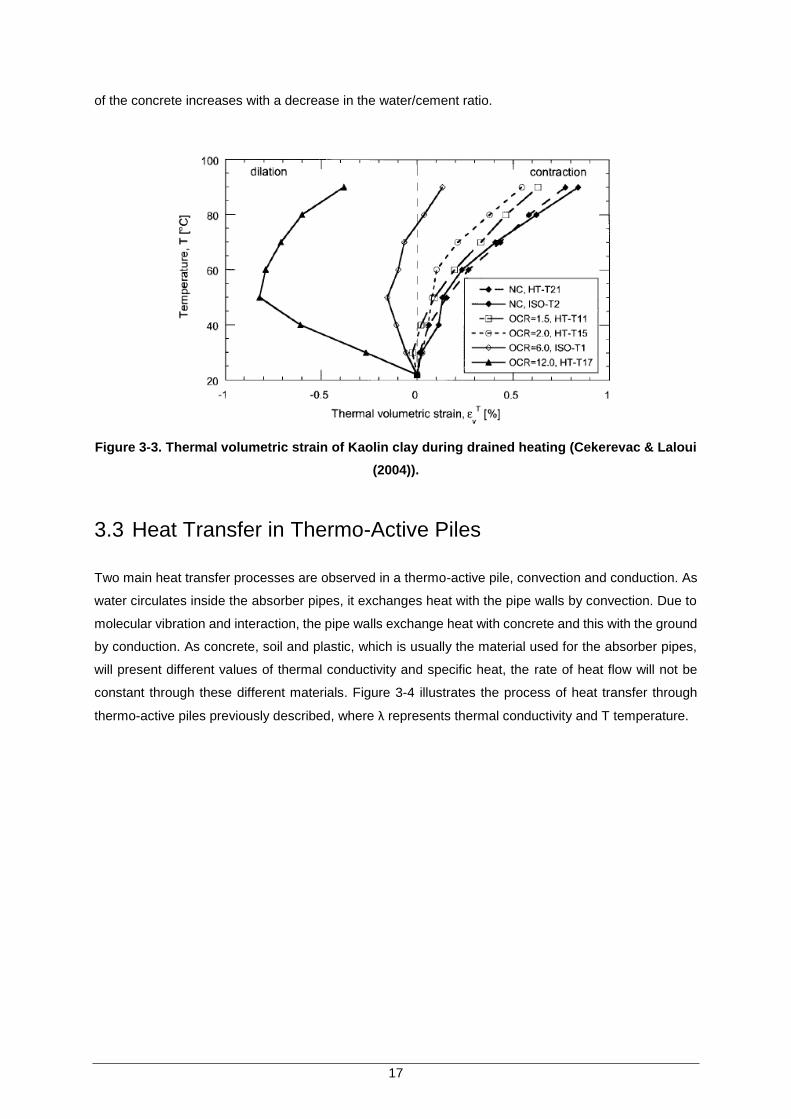
expansive behaviour which increases with OCR and is followed by plastic contraction as illustrated in
Figure 3-3. This means that clays can present positive or negative thermal expansion coefficients
depending mainly on their OCR values but also on their mineralogical properties and the temperature
magnitudes they are subjected to.
As with most construction materials and unlike soil, concrete always presents a positive coefficient of
thermal expansion meaning that it will increase in volume when heated and reduce in volume when
cooled. Aggregates are the main component of concrete and have a great influence over its thermal
expansive behaviour. Different aggregate types will present different mineralogical content which will
make them more or less thermal expansive, for instance, siliceous aggregates present high thermal
expansion and consequently, concrete which contains these aggregates will generally also exhibit a
high thermal expansion. Tatro (2006) reports values of concrete linear CTE between 0.76E-5 m/m/K
and 1.36E-5 m/m/K, depending on the aggregate type used in its production. The water/cement ratio
also influences the thermal expansion value of the concrete as it changes the thermal expansion of the
cement past which constitutes 15 to 20% of its volume. In general, the coefficient of thermal expansion
17
of the concrete increases with a decrease in the water/cement ratio.
Figure 3-3. Thermal volumetric strain of Kaolin clay during drained heating (Cekerevac & Laloui
(2004)).
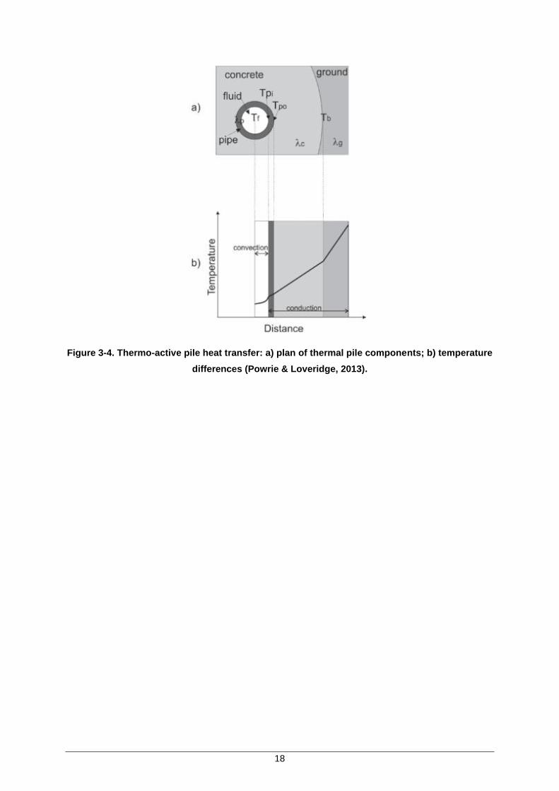
3.3 Heat Transfer in Thermo-Active Piles
Two main heat transfer processes are observed in a thermo-active pile, convection and conduction. As
water circulates inside the absorber pipes, it exchanges heat with the pipe walls by convection. Due to
molecular vibration and interaction, the pipe walls exchange heat with concrete and this with the ground
by conduction. As concrete, soil and plastic, which is usually the material used for the absorber pipes,
will present different values of thermal conductivity and specific heat, the rate of heat flow will not be
constant through these different materials. Figure 3-4 illustrates the process of heat transfer through
thermo-active piles previously described, where λ represents thermal conductivity and T temperature.
18
Figure 3-4. Thermo-active pile heat transfer: a) plan of thermal pile components; b) temperature
differences (Powrie & Loveridge, 2013).

19
Chapter 4
The Effect of Heating and
Cooling of a Pile
4 The Effect of Heating and Cooling of a Pile
This chapter gives an overview of what is to be expected in terms of developed strains and stresses in
a pile when it is subjected to a temperature change, as well as the base theory which describes their
development. The results of prominent field studies and numerical analyses performed on thermo-active
piles will then be analysed and compared to the theoretical base initially presented.

20
4.1 Thermally Induced Deformation – General Principles
When a body is subjected to a temperature change, it will attempt to expand if heated or contract if
cooled. If the body is free to expand/contract it will change in volume without any development of
additional stresses. However, if the body is partially or fully restrained thermally induced stresses will
develop, whose magnitude will be proportional to the amount of restraint the body is subjected to.
The following sub-sections give an overview of what is to be expected in terms of thermally induced
stresses on a pile which is subjected to three different restraint levels: no restraint (free body), perfect
restraint and partial restraint.
4.1.1 Free Body Response (No Restraint)
When heated or cooled, a free body will expand or contract proportionally to its coefficient of linear
thermal expansion, α (𝑚/𝑚/𝐾), and to the applied change in temperature, ∆𝑇, as expressed by Equation
4-1, where 𝜀𝑇−𝐹𝑟𝑒𝑒 represents the free thermal strain.
𝜀𝑇−𝐹𝑟𝑒𝑒 = 𝛼∆𝑇 (Equation 4-1)
The resulting geometry change, due to the thermal load can be written as:
∆𝐿 = 𝐿0 𝜀𝑇−𝐹𝑟𝑒𝑒 (Equation 4-2)
Since the body is free to expand/contract, it will change in geometry without mobilizing any additional
stresses. Figure 4-1 illustrates the previous statement, considering a pile as the free body.
Figure 4-1. Thermal response of a non-restrained pile (free body): a) heating; b) cooling
(Bourne-Webb, et al., 2013).
21
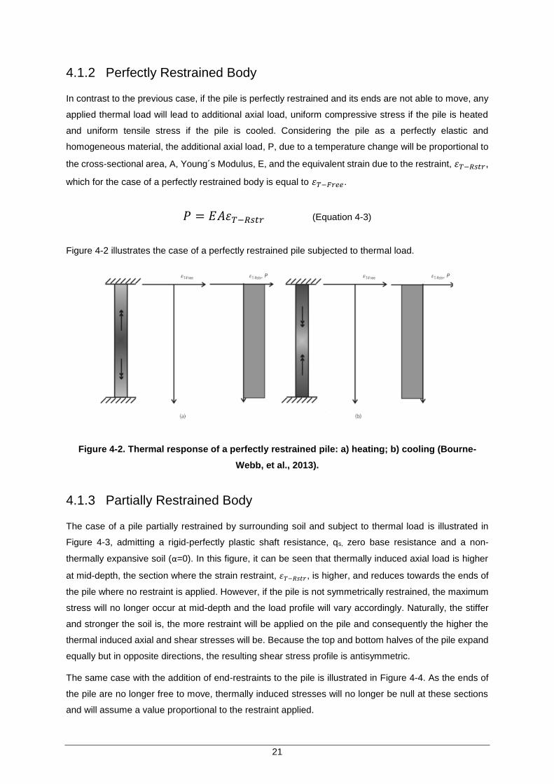
4.1.2 Perfectly Restrained Body
In contrast to the previous case, if the pile is perfectly restrained and its ends are not able to move, any
applied thermal load will lead to additional axial load, uniform compressive stress if the pile is heated
and uniform tensile stress if the pile is cooled. Considering the pile as a perfectly elastic and
homogeneous material, the additional axial load, P, due to a temperature change will be proportional to
the cross-sectional area, A, Young´s Modulus, E, and the equivalent strain due to the restraint, 𝜀𝑇−𝑅𝑠𝑡𝑟,
which for the case of a perfectly restrained body is equal to 𝜀𝑇−𝐹𝑟𝑒𝑒.
𝑃 = 𝐸𝐴𝜀𝑇−𝑅𝑠𝑡𝑟 (Equation 4-3)
Figure 4-2 illustrates the case of a perfectly restrained pile subjected to thermal load.
Figure 4-2. Thermal response of a perfectly restrained pile: a) heating; b) cooling (Bourne-
Webb, et al., 2013).
4.1.3 Partially Restrained Body
The case of a pile partially restrained by surrounding soil and subject to thermal load is illustrated in
Figure 4-3, admitting a rigid-perfectly plastic shaft resistance, qs, zero base resistance and a non-
thermally expansive soil (α=0). In this figure, it can be seen that thermally induced axial load is higher
at mid-depth, the section where the strain restraint, 𝜀𝑇−𝑅𝑠𝑡𝑟, is higher, and reduces towards the ends of
the pile where no restraint is applied. However, if the pile is not symmetrically restrained, the maximum
stress will no longer occur at mid-depth and the load profile will vary accordingly. Naturally, the stiffer
and stronger the soil is, the more restraint will be applied on the pile and consequently the higher the
thermal induced axial and shear stresses will be. Because the top and bottom halves of the pile expand
equally but in opposite directions, the resulting shear stress profile is antisymmetric.
The same case with the addition of end-restraints to the pile is illustrated in Figure 4-4. As the ends of
the pile are no longer free to move, thermally induced stresses will no longer be null at these sections
and will assume a value proportional to the restraint applied.

22
Figure 4-3. Thermal response of a pile laterally restrained: (a) heating; (b) cooling (Bourne-
Webb, et al., 2013).
Figure 4-4. Thermal response of a pile laterally and end restrained: (a) heating; (b) cooling
(Bourne-Webb, et al., 2013).
The typical response of a friction pile subjected to a mechanical load with no end-restraints considered
is illustrated in Figure 4-5(a). Figure 4-5(b) and (c) illustrate the effects of a subsequent thermal load
on the pile, heating and cooling respectively, which are the summation of the effects indicated in Figure
4-3 on the mechanical load transfer profile illustrated in Figure 4-5(a).

23
Figure 4-5. Combined mechanical and thermal load effects on a partially restrained pile. Dash-
dotted lines represent the effect of stronger thermal load or pile restraint. (a) Mechanical load
only; (b) combined mechanical load and heating; (c) combined mechanical load and cooling;
(Bourne-Webb, et al., 2013).
While the concepts previously mentioned are very straight forward and easily understandable, in reality,
the problem of a thermally loaded foundation pile is of great complexity. Soil is generally highly
heterogeneous and therefore, the restraint it will induce in the pile will most likely change in depth. As
the soil will also be heated/cooled together with the pile, it will also experience expansion/contraction,
and the relationship between the concrete and soil thermal expansion values is likely to play a role in
the resulting behaviour. A further look into thermal pile behaviour and an overview of past field
experiments is now made.
4.2 Experimental Observations of the Effect of Heating and
Cooling a Pile
In this section, the results of two tests performed on energy piles located in Lausanne, Switzerland and
South London, United Kingdom are analysed. These tests were conducted with the aim of improving
our knowledge regarding the impact of the thermal load on the geotechnical performance of pile
foundations. The documentation of observational results is also important as these allow numerical
models to be validated, i.e. to evaluate the ability of the models to recreate the behaviours we see in
reality.
4.2.1 École Polytechnique Fédérale de Lausanne
The results of an in situ test carried on an energy pile at the École Polytechnique Fédérale de Lausanne
(EPFL) in Switzerland, were reported by Laloui et al., (2006). The tested pile was located at the side of
a 100 m long by 30 m wide building. The nominal pile diameter was 88 cm and its depth 25.8 m, the soil
stratigraphy was complex and after various geotechnical investigations five different soil layers were
identified (Figure 4-6). Over the top half of the pile, alluvial soil was identified while in the bottom half,
24
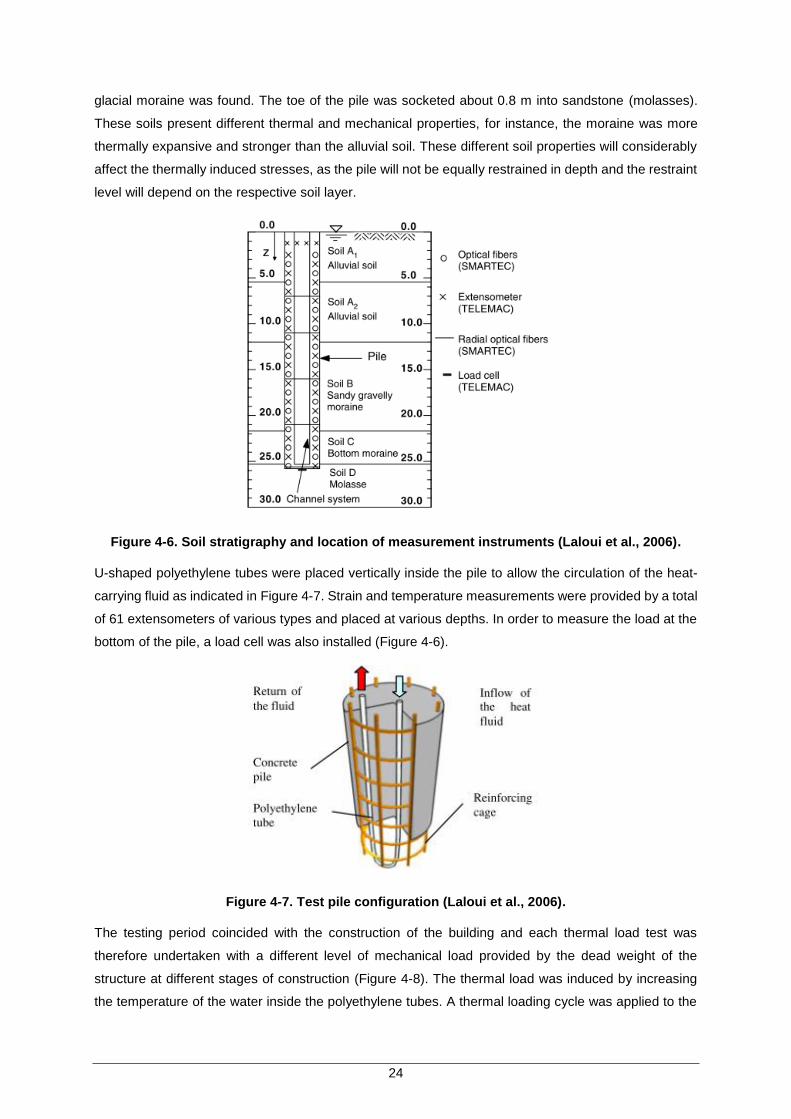
glacial moraine was found. The toe of the pile was socketed about 0.8 m into sandstone (molasses).
These soils present different thermal and mechanical properties, for instance, the moraine was more
thermally expansive and stronger than the alluvial soil. These different soil properties will considerably
affect the thermally induced stresses, as the pile will not be equally restrained in depth and the restraint
level will depend on the respective soil layer.
Figure 4-6. Soil stratigraphy and location of measurement instruments (Laloui et al., 2006).
U-shaped polyethylene tubes were placed vertically inside the pile to allow the circulation of the heat-
carrying fluid as indicated in Figure 4-7. Strain and temperature measurements were provided by a total
of 61 extensometers of various types and placed at various depths. In order to measure the load at the
bottom of the pile, a load cell was also installed (Figure 4-6).
Figure 4-7. Test pile configuration (Laloui et al., 2006).
The testing period coincided with the construction of the building and each thermal load test was
therefore undertaken with a different level of mechanical load provided by the dead weight of the
structure at different stages of construction (Figure 4-8). The thermal load was induced by increasing
the temperature of the water inside the polyethylene tubes. A thermal loading cycle was applied to the

25
pile at the end of the construction of each story. In addition to the measurements made during the casting
of the pile (Test 0), a total of seven tests were carried out. The loading history of the pile can be seen in
Figure 4-8; Test 1 was started in May 1998 and Test 7 completed in April 1999.
Test 1 differs from the subsequent tests since at this stage the restraint at the pile head was low as only
the substructure of the building was in place at the time, while in the remaining tests, pile head restraint
is considerably higher due to the construction of the building structure. Test 1 was also subjected to a
higher thermal load (∆𝑇 = 21°𝐶) than the following tests (∆𝑇 = 15°𝐶). A finite element thermo-
mechanical model of the test pile was also developed with the aim of recreating the observed
experimental results.
Figure 4-8. Thermo-mechanical loading history (Laloui et al., 2006).
4.2.1.1 Thermally Induced Stresses (Test 1)
As previously mentioned, during Test 1 no mechanical load other than the self-weight of the pile was
applied and a heating-cooling cycle was imposed (12 days of heating then 16 days of natural cooling)
as indicated by Figure 4-9. At this stage the restraint on the pile head was also diminished as only the
substructure of the building was constructed. While the head of the pile was largely free to move, the
pile was partially restrained along the pile shaft by the development of friction on the pile-soil interface
and at the toe due to the presence of the sandstone. As the pile cannot expand freely, thermally induced
stresses are expected to develop. Figure 4-10 illustrates the axial stress changes in the pile during Test
1 when it was subjected to a temperature increase of 13.4ºC.

26
Figure 4-9. Temperature values imposed in the pile (Laloui et al., 2006).
Figure 4-10. Thermal vertical stresses under a thermal load of 13.4ºC (Laloui et al., 2006).
The heating thermal load led to the development of significant compressive stresses in the pile reaching
a maximum value of about 3 MPa. It was also assessed that as the surrounding types of soil changed
so did the stress levels, which can be seen in Figure 4-10, where the soil layers A, B,C and D can be
identified. The thermal loading also led to a maximum uplift of the pile of about 4 mm.
4.2.1.2 Thermal-mechanical behaviour of the pile (Test 7)
During test 7, the pile was under mechanical load due to the weight of the completed building which led
to a vertical stress of about 1.3 MPa at the pile head, the load was carried entirely on the pile shaft with
the toe carrying almost no load, “Mech.” in Figure 4-11(a). The effect of the thermal load (T = +15°C)
was quite significant as it led to a considerable compressive overstress of about 1.2 MPa at the pile
head and 2 MPa at the toe (“Mech.+Ther”, Figure 4-11(a)).

27
Figure 4-11. Thermo-mechanical vertical stresses in the pile: (a) experimental results; (b)
numerical simulations).
Comparing the results from Figure 4-11 (a) to the ones idealized in Figure 4-5, the influence of the soil
non-homogeneity over the thermally induced stresses can clearly be seen. Due to different resistance
and thermal expansion properties, different soil types will induce different levels of restraint on the pile
as they will mobilize different levels of interface shear stress and therefore lead to different thermally
induced stresses.
The effect of the pile’s end restraint can also be seen, in Figure 4-5 no end restraints are applied to the
pile and therefore no thermal stresses develop in these sections. However, the pile in Figure 4-11 is
restrained at its head due to the building structure above it and at its toe due to it being socketed in the
sandstone. This restraint led to considerable thermally induced stress in these sections.
Laloui et al. (2006) concluded that the numerical model was found able to reproduce the complex
behaviour of the energy pile and reproduced well the experimental results. However, comparing Figure
4-11(a) and (b), it can be observed that the previous statement is only true to some extent. Some flaws
can be pointed in the numerical model results, especially the reproduction of the stresses induced by
the mechanical load and the magnitude of the predicted thermal stresses at the pile’s head which were
considerably lower than those measured experimentally.
4.2.2 Lambeth College, London
Situated within the grounds of the Clapham Centre of Lambeth College in South London, this test pile
was carried as part of a project which involves the construction of a new five-storey building. The
observational results from this test pile were reported by Bourne-Webb et al., 2009. The new building is
supported on bored pile foundations with 143 piles of 600 mm nominal diameter, which also incorporate
heat exchange pipe loops for use in the ground-source heat-pump system. In order to better understand
the impact of the thermal load over the pile’s mechanical behaviour, a 23 m long, 600 mm diameter test
pile was loaded to a nominal working load of 1200 kN and then subjected to cycles of heating (input
temperature of +56⁰C) and cooling (input temperature of -6⁰C).
28
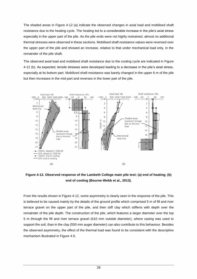
The shaded areas in Figure 4-12 (a) indicate the observed changes in axial load and mobilised shaft
resistance due to the heating cycle. The heating led to a considerable increase in the pile’s axial stress
especially in the upper part of the pile. As the pile ends were not highly restrained, almost no additional
thermal stresses were observed in these sections. Mobilised shaft resistance values were reversed over
the upper part of the pile and showed an increase, relative to that under mechanical load only, in the
remainder of the pile shaft.
The observed axial load and mobilised shaft resistance due to the cooling cycle are indicated in Figure
4-12 (b). As expected, tensile stresses were developed leading to a decrease in the pile’s axial stress,
especially at its bottom part. Mobilized shaft resistance was barely changed in the upper 6 m of the pile
but then increases in the mid-part and reverses in the lower part of the pile.
Figure 4-12. Observed response of the Lambeth College main pile test: (a) end of heating; (b)
end of cooling (Bourne-Webb et al., 2013).
From the results shown in Figure 4-12, some asymmetry is clearly seen in the response of the pile. This
is believed to be caused mainly by the details of the ground profile which comprised 5 m of fill and river
terrace gravel on the upper part of the pile, and then stiff clay which stiffens with depth over the
remainder of the pile depth. The construction of the pile, which features a larger diameter over the top
5 m through the fill and river terrace gravel (610 mm outside diameter), where casing was used to
support the soil, than in the clay (550 mm auger diameter) can also contribute to this behaviour. Besides
the observed asymmetry, the effect of the thermal load was found to be consistent with the descriptive
mechanism illustrated in Figure 4-5.

29
4.3 Numerical Analysis of the Effect of Heating and Cooling a
Pile
Few numerical studies have yet been published regarding the thermal-mechanical behaviour of energy
piles. In this section, we will take a look at some of these studies and their respective findings and
conclusions, some of which have been further investigated in this thesis.
4.3.1 Bodas Freitas et al., 2013 and Cruz Silva, 2012
Bodas Freitas et al. (2013) and Cruz Silva (2012), describe the development of an axisymmetric
numerical model in the finite element software ADINA. A single pile with diameter of 1 m and length of
30 m was considered, the side and bottom boundaries of the finite element mesh were set at a distance
of 60 m and 90 m respectively. Both the concrete making up the pile and the surrounding soil were
considered as purely elastic materials with Young modulus of 30 GPa and 30 MPa respectively. Even
though the soil Young modulus base value was 30 MPa an increase in this value to 60 MPa was also
tested. The concrete coefficient of volumetric thermal expansion, was set to 3.0𝐸−5𝐾−1, while three
different values of the same parameter were tested for the soil: 0, 1.5𝐸−5 and 6.0𝐸−5𝐾−1. The
mechanical load applied to the pile (about 4.7 MN) was modelled by applying a boundary pressure of 6
MPa at the pile’s head, and the thermal load, by the application of an increment of temperature ∆𝑇 =
+30°𝐶 to all elements making up the pile, under steady state heat flow conditions.
The effect of the relationship between pile and soil coefficient of volumetric thermal expansion, the
stiffness of the soil and the thermal boundary condition on the ground surface were assessed in this
study. While a change in the thermal boundary condition on the ground surface won’t affect the
temperature of the pile, it will have a significant effect on the temperature of the surrounding soil (Figure
4-13), as the soil itself will contract or expand due to thermal load, this change will affect the pile-soil
interaction.
Figure 4-13. Steady-state temperature field as function of surface thermal boundary condition
(contour interval: 2ºC) (Bodas Freitas et al., 2013).

30
The results in terms of change in pile axial stress and pile-soil interface shear stress due to the thermal
load of +30°𝐶 are plotted in Figures 4-14 and 4-15 respectively.
Figure 4-14. Change in pile axial stress due to temperature change of +𝟑𝟎°𝑪 (Bodas Freitas et
al., 2013).
Figure 4-15. Change in pile-soil interface shear stress due to temperature change of +𝟑𝟎°𝑪
(Bodas Freitas et al., 2013).
From the above results, the following conclusions were made:
Changing the soil coefficient of thermal expansion has a big impact on the resulting thermally
induced stresses in the pile. When the soil was more expansive than the concrete (𝛽𝑠𝑜𝑖𝑙 =
6𝐸−5𝐾−1𝑎𝑛𝑑 𝛽𝑐𝑜𝑛𝑐𝑟𝑒𝑡𝑒 = 3𝐸−5 𝐾−1) tensile axial stresses developed for the case of an adiabatic

31
surface, Figure 4-14 (a), while in the remaining cases (lower values of 𝛽soil and constant
temperature surface), heating led to compressive stresses;
The applied ground surface thermal boundary condition impacts heavily the results if the soil is
more thermally expansive than the concrete;
An increase in soil Young modulus led to an increase in the thermally induced stresses, which
was expected as a stiffer soil will impose more restraint on the pile.
Understanding in greater detail the relationship between the concrete and soil thermal expansion values,
as well as the influence of the ground surface thermal boundary condition, is the main aim of this thesis
and is further investigated in Chapters 5 and 6.
4.3.2 Di Donna et al., 2013
Di Donna et al. (2013) developed a numerical model with thermo-hydro-numerical coupling of a group
of thermally-activated piles connected to a ground slab, which aimed to investigate the effects of cyclic
temperature variations on the different aspects involved in the geotechnical design of thermally-
activated pile foundations.
The foundation modelled comprised 150 piles with a diameter of 80 cm and a length of 20 m which were
spaced 7 m apart in both directions. The slab was 110 m long and had a thickness of 0.5 m. Due to the
symmetry of the problem and for simplicity reasons only, the numerical model was limited to 4 piles in
2D plane strain conditions (Figure 4-16). However, this simplification involves considering a circular pile
as an infinite wall in the plane perpendicular to the one of the simulation. To account for this
consideration, the pile axial stiffness was adjusted to an equivalent Young modulus, other parameters
such as porosity and thermal conductivity were also adjusted to weighted average values. Because the
deformation in the third direction is also prevented, the thermal expansion coefficient of the pile was also
adjusted to the real one divided by (1+ѵ).
Figure 4-16. Numerical model: geometry, mesh and boundary conditions (Di Donna et al.,
2013).

32
Both the concrete and the soil were considered as porous materials with a liquid and solid phase, and
the whole medium was considered as fully saturated. The piles and slab are made of concrete which
behaves thermo-elastically while the soil behaviour was simulated by a thermoelastic-thermoplastic
constitutive model named ACMEG-T which allows for the consideration of thermal cyclic effects on the
response of the material. Taking into consideration both the liquid and the solid phases, the soil
presented a linear coefficient of thermal expansion of 3 m/m/K and the concrete 1.856 m/m/K, meaning
that soil was approximately twice as thermally expansive as concrete. The pile-soil interface was set to
behave according to the same ACMEG-T model with the same parameters as the soil but a lower angle
of shearing resistance. Thermal loading of the piles was achieved by applying a heat flux in heating and
cooling equivalent to 150 W/m along the pile.
The initial temperature of both soil and piles was set to 11ºC while the temperature of the slab was fixed
at 15ºC throughout the computation which aimed to simulate a regulated temperature in the interior of
the building. The remaining thermal boundary conditions of the model were set to be adiabatic.
Figure 4-17 shows the thermally induced displacements of the foundation through time due to the cyclic
thermal load. Two phenomena were observed: One is cyclic vertical displacements of the foundation
due to elastic dilative behaviour of the soil, which is reversible during cooling, and makes the foundation
move upwards during heating and downwards during cooling. The other is an irreversible displacement
induced by the cyclic thermal loading due to an increase in the soil pore water pressure during the
heating phase and the following consolidation. The irreversible displacement induced a settlement of
0.3 cm (12% of the settlement induced by the mechanical load) while the elastic cyclic settlement had
an amplitude of 0.6 cm. Because all the piles were heated and cooled equally no differential settlements
were induced by the thermal load, however, according to the Di Donna et al. (2013), if thermal load is
not equal to all piles potential differential cyclic settlements problems may occur.
Figure 4-17. Thermally induced displacement of the foundation (Di Donna et al., 2013).
Figure 4-18 shows the evolution through time of the thermally induced vertical stresses in Pile 2 (Figure
4-16) at the end of a heating phase. As previously described in Section 4.1, pile heating led to an
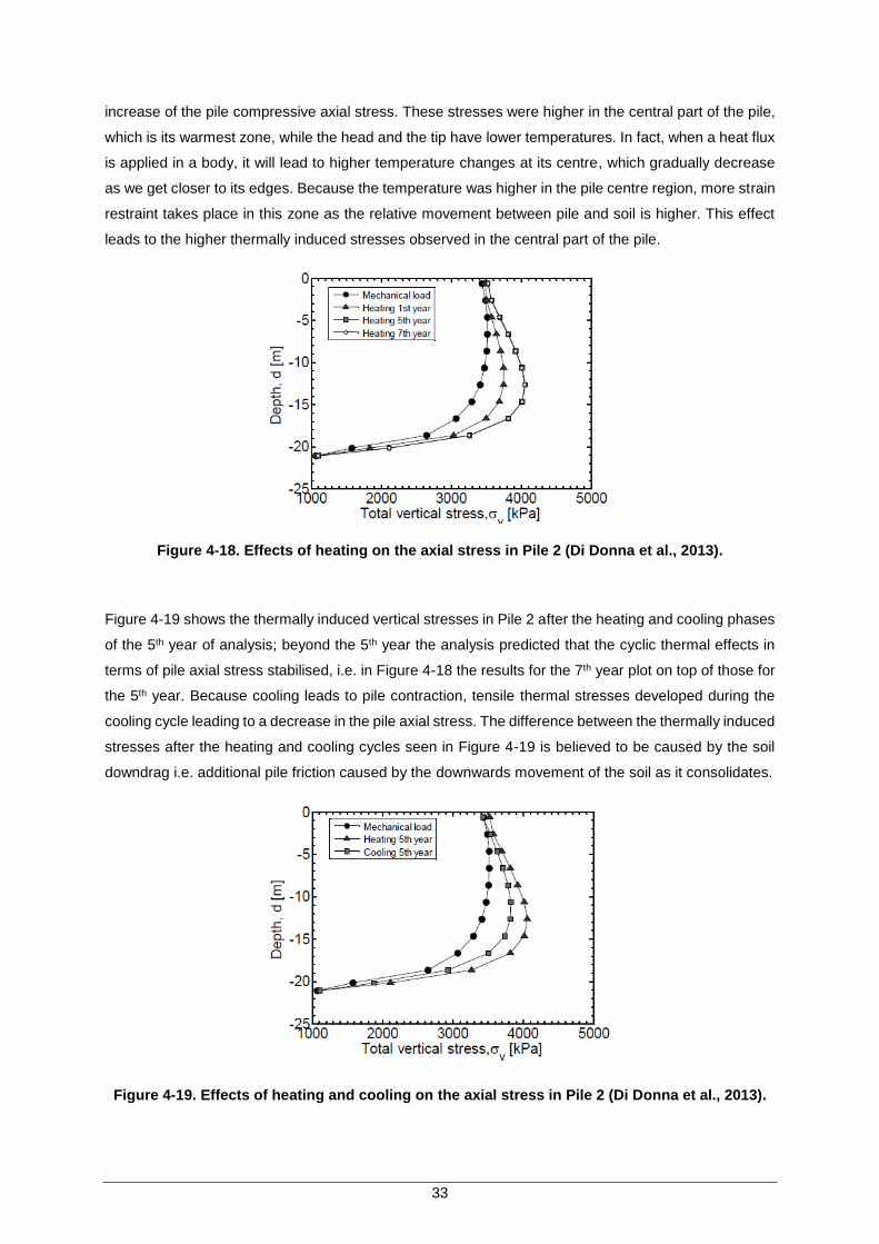
33
increase of the pile compressive axial stress. These stresses were higher in the central part of the pile,
which is its warmest zone, while the head and the tip have lower temperatures. In fact, when a heat flux
is applied in a body, it will lead to higher temperature changes at its centre, which gradually decrease
as we get closer to its edges. Because the temperature was higher in the pile centre region, more strain
restraint takes place in this zone as the relative movement between pile and soil is higher. This effect
leads to the higher thermally induced stresses observed in the central part of the pile.
Figure 4-18. Effects of heating on the axial stress in Pile 2 (Di Donna et al., 2013).
Figure 4-19 shows the thermally induced vertical stresses in Pile 2 after the heating and cooling phases
of the 5th year of analysis; beyond the 5th year the analysis predicted that the cyclic thermal effects in
terms of pile axial stress stabilised, i.e. in Figure 4-18 the results for the 7th year plot on top of those for
the 5th year. Because cooling leads to pile contraction, tensile thermal stresses developed during the
cooling cycle leading to a decrease in the pile axial stress. The difference between the thermally induced
stresses after the heating and cooling cycles seen in Figure 4-19 is believed to be caused by the soil
downdrag i.e. additional pile friction caused by the downwards movement of the soil as it consolidates.
Figure 4-19. Effects of heating and cooling on the axial stress in Pile 2 (Di Donna et al., 2013).
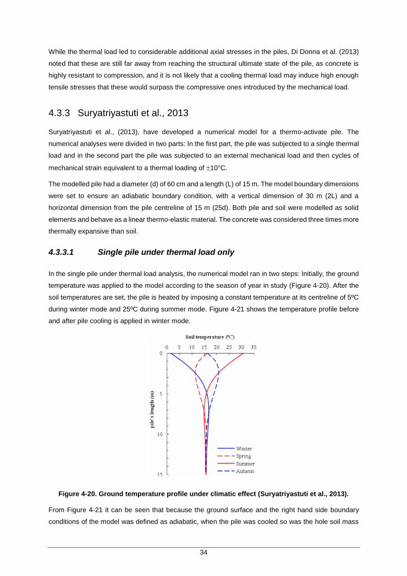
34
While the thermal load led to considerable additional axial stresses in the piles, Di Donna et al. (2013)
noted that these are still far away from reaching the structural ultimate state of the pile, as concrete is
highly resistant to compression, and it is not likely that a cooling thermal load may induce high enough
tensile stresses that these would surpass the compressive ones introduced by the mechanical load.
4.3.3 Suryatriyastuti et al., 2013
Suryatriyastuti et al., (2013), have developed a numerical model for a thermo-activate pile. The
numerical analyses were divided in two parts: In the first part, the pile was subjected to a single thermal
load and in the second part the pile was subjected to an external mechanical load and then cycles of
mechanical strain equivalent to a thermal loading of 10°C.
The modelled pile had a diameter (d) of 60 cm and a length (L) of 15 m. The model boundary dimensions
were set to ensure an adiabatic boundary condition, with a vertical dimension of 30 m (2L) and a
horizontal dimension from the pile centreline of 15 m (25d). Both pile and soil were modelled as solid
elements and behave as a linear thermo-elastic material. The concrete was considered three times more
thermally expansive than soil.
4.3.3.1 Single pile under thermal load only
In the single pile under thermal load analysis, the numerical model ran in two steps: Initially, the ground
temperature was applied to the model according to the season of year in study (Figure 4-20). After the
soil temperatures are set, the pile is heated by imposing a constant temperature at its centreline of 5ºC
during winter mode and 25ºC during summer mode. Figure 4-21 shows the temperature profile before
and after pile cooling is applied in winter mode.
Figure 4-20. Ground temperature profile under climatic effect (Suryatriyastuti et al., 2013).
From Figure 4-21 it can be seen that because the ground surface and the right hand side boundary
conditions of the model was defined as adiabatic, when the pile was cooled so was the hole soil mass

35
at the top of the model. This is however an unrealistic situation, in reality, the ground surface temperature
will be imposed by the temperature of the overlying structure and the outside air temperature and should
remain almost unchanged after the cooling thermal load is applied to the pile. The temperature profiles
illustrated in Figure 4-13 are believed to better represent the effect of the pile heating in the surrounding
soil temperature.
Figure 4-21. Ground temperature profile in the winter mode: (a) the initial conditions. (b) at the
end of the thermal load (Suryatriyastuti et al., 2013).
Figure 4-22 (a) and (b) illustrate the thermally induced mechanical behaviour of the pile in terms of
developed axial stress and axial displacement respectively. The heating thermal load led to pile
expansion and the development of compressive stresses as part of this expansion is restrained by the
surrounding soil, while the cooling thermal load led to the opposite behaviour. These results are in
accordance to the theoretical ones previously described (Figure 4-3), with the difference that in this case
the pile is partially restrained at its base by the soil, leading to non-symmetrical stress and displacement
profiles.
Figure 4-22. Thermally induced mechanical behaviour of the pile at winter and summer mode:
(a) thermal axial force (b) thermal axial displacement (Suryatriyastuti et al., 2013).

36
4.3.3.2 Combined mechanical and cyclic thermal loading
In this analysis, the pile is initially mechanically and incrementally loaded up to 33% of its ultimate static
load resistance. After the mechanical load is applied, cycles of mechanical strain equivalent to a thermal
loading of 10°C were imposed on the pile. The magnitude of the strain cycles was calculated according
to Equation 4-1 (free thermal strain) which admits that no restraint is applied to the pile. Some criticism
can be made regarding this decision since by simulating the thermal load with additional strains in the
pile and not actually by heating and cooling it, part of the thermal-mechanical interaction between the
pile and soil is lost, and implies that the soil is unaffected by temperature change. A total of 24 cycles of
strain were applied to the pile starting with strain equivalent to a cooling cycle and followed by strain
equivalent to a heating cycle. Interface elements were introduced at the pile-soil contact zone following
a constitutive interface law called Modjoin which is capable of modelling cyclic degradation phenomena.
Figure 4-23 shows the evolution of the pile head settlement due to the thermal cycles. The cooling
thermal load led to contraction of the pile and therefore an increase in the pile head settlement while the
opposite behaviour happened when a heating cycle took place. At the end of all the thermal cyclic
loading, an additional plastic settlement of 3 mm (7% of the settlement induced by the mechanical load)
was verified due to the degradation of the pile-soil interface resistance through the thermal cycles.
Figure 4-23. Cyclic variation in the pile head displacement (Suryatriyastuti et al., 2013).
Figure 4-24 illustrates the axial normal force on the pile at the beginning and at the end of the thermal
cycles. It was observed that the variation in normal force increased more in heating cycles than in cooling
ones, this happens because when the pile is expanding the pile-soil interface generated more restraint
than when it contracts. At the end of the 24th cycle, a maximum normal force increase of 16% relative to
the value induced by the mechanical load was predicted.

37
Figure 4-24. Thermally induced normal force at the beginning and at the end of the thermal
cycles (Suryatriyastuti et al., 2013).
Suryatriyastuti et al. (2013) concluded that the cyclic degradation of the mechanical resistance of
thermally actived piles is not negligible and should be taken into account in the geotechnical design of
such piles. While this conclusion is true for the particular set of parameters used, no evidence of cyclic
thermal degradation in thermo-active piles has yet been demonstrated in reality and the cyclic
degradation reported in this study is probably a mere consequence of the constitutive law adopted for
the interface.

38
39
Chapter 5
Thermal Analysis
5 Thermal Analysis
In this chapter the results of a series of numerical thermal analyses are presented and discussed. These
analyses were performed in order to better understand the pile-soil interaction problem from a purely
thermal point of view, and to determine some of the thermal properties of the numerical thermal-
mechanical model used in Chapter 6.

40
5.1 Introduction
In the analysis of the response of thermally activated pile foundations, a complex interaction resulting
from the temperature field (and especially the surface temperature) and the thermal and mechanical
properties of the pile and the soil, in particular the coefficient of thermal expansion, has been highlighted
(Bodas Freitas et al. 2013, Cruz Silva, 2012).
In this section, and in order to better understand the first part of this interaction problem (i.e. the
temperature field), the heat exchanger pile problem was studied from a purely thermal point of view and
the following aspects were investigated:
The simulation of the pile thermal load in a numerical model;
The effect of soil and concrete thermal conductivity values;
Heat loss through ground slabs and ground surface temperature.
Some of the findings and conclusions reported in this section are later implemented in a thermal-
mechanical numerical model (Chapter 6) in order to investigate their influence in the thermo-mechanical
response of a pile.
5.2 Thermal Load through the Pile
Thermal load on piles is often simulated in numerical models by applying a constant temperature
increase or a heat flux to all elements or nodes constituting the pile. In reality, heat flows from absorber
pipes which are either placed close to the centreline of the pile or close to the pile edge where the pipes
are attached to the reinforcement cage. (Figure 5-1). This means that the temperature in the pile is not
uniform and tends to be higher near the pipes, where the heat exchange fluid circulates, and reduces
with distance from them.
Figure 5-1. Usual thermo-active pile construction details: (a) absorber pipes fixed to a pile
reinforcement; (b) absorber pipes installed in the centre of the pile (Powrie & Loveridge, 2013).

41
The main objectives of the analyses performed in this section are to assess how the heating of the pile
is simulated affects the temperature field of the model and if the pile thermal load can be simplified by
the application of constant temperature or a heat flux all over the pile or if the absorber pipe geometry
should be modelled.
In order to look at the temperature fields both in depth and in plan, two finite element models were
developed using the software Abaqus: one was axisymmetric and the other two-dimensional (2D).
Alternatively it would also be possible to create a single 3D model but due to the added complexity that
this required, the former option was preferred.
5.2.1 Axisymmetric Thermal Model
In many cases, piles are axisymmetric bodies and they can be numerically modelled by an axisymmetric
2D model. While presenting identical results, the use of an axisymmetric model instead of a 3D model
presents a considerable advantage in terms of calculation time because the 3D model will require a
much higher number of finite elements.
The pile has a diameter of 1 m and is 30 m deep, the bottom and side boundaries of the finite element
model were set at a distance of 90 m (3L) and 60 m (2L) respectively. Bottom and side thermal
boundaries were defined at a constant 12ºC in accordance to Figure 2-1, while the top boundary was
defined as having no heat flux (adiabatic) since in this study we don’t want to take into consideration the
effect of the outside temperature. All the elements in the model have an initial temperature of 12ºC.The
geometry, boundary conditions and mesh configuration of the model are indicated in Figure 5-2. Two
different materials, concrete and soil, whose thermal properties are indicated in Table 5-1 were created.
The pile is modelled with solid elements assigned the properties for concrete while the surrounding
ground is modelled with solid elements assigned the properties for soil. Since only thermal conduction
will take place in the model, no mechanical properties need to be specified.
Soil Concrete
Thermal Conductivity ,k (𝑾/𝒎. 𝑲) 1 2
Specific Heat, 𝒄 ( 𝑱/𝒌𝒈. 𝑲) 1220 940
Density, ρ (𝒌𝒈/𝒎𝟑) 1600 2450
Table 5-1. Soil and concrete thermo-physical properties used in the base analysis.
In Abaqus, in order for two bodies in contact to transfer heat by conduction, an interface thermal
conductance value must be defined, which is a property that indicates the ability of an interface to
conduct heat. As soil is a granular material and concrete has a rough surface, a perfect contact between
these bodies is impossible to achieve and thermal resistance will develop in this interface mainly due to
voids existing between the two surfaces. Interface thermal conductance is defined as the ratio between
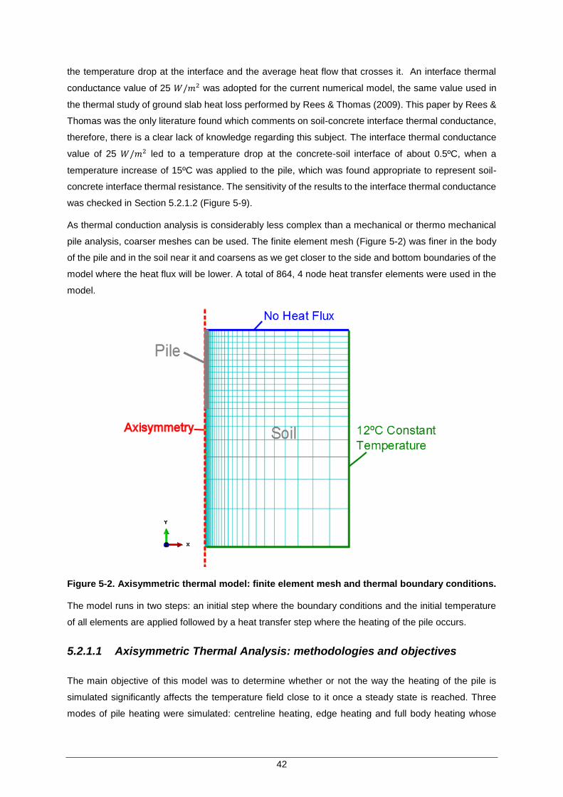
42
the temperature drop at the interface and the average heat flow that crosses it. An interface thermal
conductance value of 25 𝑊/𝑚2 was adopted for the current numerical model, the same value used in
the thermal study of ground slab heat loss performed by Rees & Thomas (2009). This paper by Rees &
Thomas was the only literature found which comments on soil-concrete interface thermal conductance,
therefore, there is a clear lack of knowledge regarding this subject. The interface thermal conductance
value of 25 𝑊/𝑚2 led to a temperature drop at the concrete-soil interface of about 0.5ºC, when a
temperature increase of 15ºC was applied to the pile, which was found appropriate to represent soil-
concrete interface thermal resistance. The sensitivity of the results to the interface thermal conductance
was checked in Section 5.2.1.2 (Figure 5-9).
As thermal conduction analysis is considerably less complex than a mechanical or thermo mechanical
pile analysis, coarser meshes can be used. The finite element mesh (Figure 5-2) was finer in the body
of the pile and in the soil near it and coarsens as we get closer to the side and bottom boundaries of the
model where the heat flux will be lower. A total of 864, 4 node heat transfer elements were used in the
model.
Figure 5-2. Axisymmetric thermal model: finite element mesh and thermal boundary conditions.
The model runs in two steps: an initial step where the boundary conditions and the initial temperature
of all elements are applied followed by a heat transfer step where the heating of the pile occurs.
5.2.1.1 Axisymmetric Thermal Analysis: methodologies and objectives
The main objective of this model was to determine whether or not the way the heating of the pile is
simulated significantly affects the temperature field close to it once a steady state is reached. Three
modes of pile heating were simulated: centreline heating, edge heating and full body heating whose

43
characteristics are as follows:
Centreline Heating: The pile is heated up to a constant temperature of 30°C (∆𝑇 = +18⁰𝐶) on the
centreline over its full length. (Figure 5-3 (a)). This heating mode aims to simulate the case where
the absorber pipes are placed in the centre of the pile Figure 5-1 (b).
Edge Heating: The pile is heated up to 30°C (∆𝑇 = +18⁰𝐶) along a line which runs the depth of
the pile and is located at a distance of 0.375 m (0.75R) from the pile centreline (Figure 5-3 (b)). This
heating mode aims to simulate the case where the absorber pipes are attached to the reinforcement
cage, close to the edge of the pile. Figure 5-1 (a).
Full Body Heating: All elements making up the pile are heated to 30°C (∆𝑇 = +18⁰𝐶) (Figure 5-3
(c)).This is the heating mode usually adopted in many published numerical studies of thermal active
piles.
Figure 5-3. Modes of heating: (a) centreline heating; (b) edge heating; (c) full body heating.
In order to assess if the three heating modes previously described produce similar temperature fields or
not, steady state analyses were run for each of these and the results compared.
The second objective of the axisymmetric thermal study was to assess the influence of the values of
thermal conductivity assumed for the soil and concrete on the temperature fields obtained. To do so,
four steady state analyses were carried for each of the edge heating and centreline heating modes. In
each of these four analyses, soil and concrete thermal conductivity values were varied as follows:
Base Case: In the base case, soil and concrete thermal conductivity values were those indicated in
Table 5-1 (𝑘𝑐 = 2 𝑊/𝑚. 𝐾; 𝑘𝑠 = 1 𝑊/𝑚. 𝐾) and are the values that were used in the remaining
thermal analysis performed in this thesis. In the base case concrete is twice as thermally conductive
as soil.
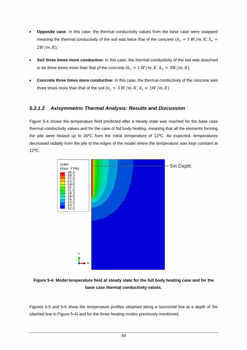
44
Opposite case: In this case, the thermal conductivity values from the base case were swapped
meaning the thermal conductivity of the soil was twice that of the concrete (𝑘𝑐 = 1 𝑊/𝑚. 𝐾; 𝑘𝑠 =
2𝑊/𝑚. 𝐾);
Soil three times more conductive: In this case, the thermal conductivity of the soil was assumed
to be three times more than that of the concrete (𝑘𝑐 = 1 𝑊/𝑚. 𝐾; 𝑘𝑠 = 3𝑊/𝑚. 𝐾);
Concrete three times more conductive: In this case, the thermal conductivity of the concrete was
three times more than that of the soil (𝑘𝑐 = 3 𝑊/𝑚. 𝐾; 𝑘𝑠 = 1𝑊/𝑚. 𝐾).
5.2.1.2 Axisymmetric Thermal Analysis: Results and Discussion
Figure 5-4 shows the temperature field predicted after a steady state was reached for the base case
thermal conductivity values and for the case of full body heating, meaning that all the elements forming
the pile were heated up to 30⁰C from the initial temperature of 12⁰C. As expected, temperatures
decreased radially from the pile to the edges of the model where the temperature was kept constant at
12⁰C.
Figure 5-4. Model temperature field at steady state for the full body heating case and for the
base case thermal conductivity values.
Figures 5-5 and 5-6 show the temperature profiles obtained along a horizontal line at a depth of 5m
(dashed line in Figure 5-4) and for the three heating modes previously mentioned.

45
Figure 5-5. Radial temperature profiles at a 5m depth.
Figure 5-6. Radial temperature profiles at a 5 m depth (zoomed closer to the pile).
It can be seen from Figures 5-5 and 5-6 that while edge heating and full body heating led to similar
temperature profiles, the difference between each being less than half a degree, centreline heating led
to considerably lower temperatures; about 5⁰C at the pile-soil interface (R=0.5 m) when compared to
the other two heating cases.
It can be concluded from these results that if the thermal pile being modelled has its absorber pipes
placed close to edge of the pile (Figure 5-1 (a)), full body heating, which is often used in numerical
simulations, will produce similar results to edge heating and is therefore a reasonable approximation.
However, if the absorber pipes are placed along the centreline of the pile (Figure 5-1 (b)), pile heating
should not be simulated as a full body heating and centreline heating should be adopted.
Figures 5-7 and 5-8 show the temperature profiles obtained alongside a horizontal line at a depth of 5
m for the four combinations of thermal conductivity values previously mentioned and for centreline
heating and edge heating modes respectively. The profiles shown are only for the first 4 m radially of
the model which include the pile section (0 to 0.5 m) and 3.5 m of surrounding soil. In these figures, kc
and ks represent the thermal conductivity of concrete and soil respectively.
0
5
10
15
20
25
30
0 10 20 30 40 50 60
Tem
per
atu
re (
⁰C)
Distance from the pile centreline (m)
Full Body Heating
Edge Heating
Centerline Heating
16
18
20
22
24
26
28
30
0,0 0,5 1,0 1,5 2,0 2,5 3,0 3,5 4,0
Tem
per
atu
re (
⁰C)
Distance from the pile centreline (m)
Full Body Heating
Edge Heating
Centerline Heating

46
Figure 5-7. Radial temperature profiles at a 5m depth with centreline heating.
Figure 5-8. Radial temperature profiles at a 5m depth with edge heating.
From Figures 5-7 and 5-8 the following conclusions can be taken:
The influence of both soil and concrete thermal conductivity was more significant for the
centreline heating case (Figure 5-7) than for the edge heating case (Figure 5-8). These results
were expected since with centreline heating, heat flows from the centre of the pile and has to
be thermally conducted through the concrete pile and into the soil while in case of edge heating,
only the concrete cover to the reinforcement cage will affect the thermal flow and the pile body
will be at a fairly constant temperature. Therefore, with full body heating and edge heating the
pile will play a lesser role in the overall heat transfer process.
An increase in concrete thermal conductivity will lead to higher temperatures overall as it will be
able to transfer heat from the heating source in the pile into the remaining elements of the pile
and into the soil more quickly. When the soil thermal conductivity is increased, the opposite
happens and lower temperatures were obtained due to the soil being able to transfer heat from
10
14
18
22
26
30
0 0,5 1 1,5 2 2,5 3 3,5 4
Tem
per
atu
re (
⁰C)
Distance from the pile's centerline (m)
Base Case (kc=2; ks=1)
Oppostie Case (kc=1; ks=2)
soil 3 times more conductive(kc=1; ks=3)
concrete 3 times moreconductive (kc=3; ks=1)

47
the model’s boundaries faster, which are at a constant 12ºC, and the model reaches a steady
state at lower temperatures.
As previously mentioned, in order for two bodies in contact to transfer heat by conduction an interface
thermal conductance value must be defined, which indicates the ability of the interface to conduct heat.
In order to evaluate the sensitivity of the results to this parameter, the temperature profiles at a depth of
5m and for different thermal conductance values were plotted (Figure 5-9). In this figure the thermal
properties of both soil and concrete are those of the base case (Table 5-1) and the pile heating method
was edge heating.
Figure 5-9.Influence of the interface thermal conductance value.
From Figure 5-9 it can be seen that the thermal conductance value of 25 W/m2 ,which was adopted for
the thermal and thermal-mechanical analyses, leads to a temperature drop at the interface of about
0.5ºC when the pile is heated from 15ºC to 30ºC. As expected, because the heat flux that reaches the
interface is constant in each of these cases, the temperature drop at the interface was proportional to
the thermal conductance value defined.
5.2.2 2D Thermal Model
As previously mentioned, a 2D thermal model was also developed in order to see temperature profiles
in plan since the previous axisymmetric model only allowed us to see temperature profiles in depth. In
the 2D thermal model, we take advantage of the bi-directional symmetry of the problem and only one
fourth of the pile and the surrounding soil is modelled. As in the axisymmetric model, the pile diameter
is 1 m and the side boundary of the model was set at a distance of 60 m. The geometry, boundary
conditions and mesh configuration of the model are indicated in Figure 5-10. The initial temperature of
all elements is set to 12⁰C.The same materials and their associated thermal properties described in
Table 5-1 were used.
18
21
24
27
30
0,0 0,5 1,0 1,5 2,0 2,5
Tem
per
atu
re (⁰
C)
Distance from the pile centerline (m)
conductance=1
conductance=2.5
conductance=10
conductance=25
conductance=100

48
Figure 5-10. 2D Thermal Model: finite element mesh, geometry and thermal boundary
conditions.
Two different pile configurations were considered:
Ring Configuration: In this configuration the pile is heated along a circular line located at a
distance of 0.75R from the pile centre (Figure 5-11). This case corresponds to what is modelled
when “edge heating” is used in an axisymmetric model (Figure 5-3 (b)).
Figure 5-11. Pile ring configuration.
Pipe Configuration: With this configuration, the aim is to model what really happens in a
thermo-active pile. As the hot water circulates through the pipes of the pile, the pipe walls will
heat and this heat will transfer by conduction to the pile and soil. A standard thermal pile

49
configuration was modelled (Figure 5-12), where the 1 m diameter pile contains 4 pairs of pipes.
The pipe diameter is 0.038 m and they are placed at a distance of 0.39 m from the pile centre
(approximating the position of the tubes when attached to the inside of a reinforcement cage).
Figure 5-12. Pile pipe configuration.
The model runs in two steps: an initial step where the boundary conditions and the initial temperature
of all elements are applied followed by a heat transfer step where the heating of the pile occurs.
5.2.2.1 2D Thermal Analysis: methodologies and objectives
The aim of these analyses was to determine whether or not the thermo-active pile problem can be
simplified and studied with an axisymmetric model where heating in the ring configuration will take place
or if the pipe layout should be modelled which would require the development of a 3D a model. Both
steady state and transient analyses were performed for the two configurations previously described,
circular and pipe layout and the resulting temperature fields compared. The initial temperatures of all
elements is 12⁰C while the temperature of the red zones indicated in Figures 5-11 and 5-12 were raised
to a constant temperature of 30⁰C (∆𝑇 = +18⁰𝐶) in order to simulate the thermal load on the pile.
5.2.2.2 2D Thermal Analysis: results and discussion
The evolution with time of the temperature field in the pile and the surrounding soil is shown in Figure
5-13. Figure 5-14 shows the evolution of the temperature at the pile-soil interface until a steady state is
reached. The temperature at the pile-soil interface is important as it is the relationship between the
temperature of the pile and the surrounding soil together with their respective thermal expansion values

50
that are expected to dictate the thermo-mechanical response of the pile-soil system.
The transient analysis highlights a considerable difference in terms of temperature levels in the pile and
surrounding soil for the two configurations studied, especially during the first weeks of heating. The pipe
configuration led to lower temperature levels in the pile than the ring configuration during the first weeks
(Figure 5-13). However, the difference between the two cases diminishes as time passes and as we get
closer to a steady state where similar temperature levels were displayed (Figure 5-14).
It can be concluded that for a steady state analysis of the thermal active pile problem, the definition of a
pipe configuration is not necessary which means that the ring configuration, typically modelled in an
axisymmetric study, is a good approximation of reality. However, if either a transient analysis is carried
out, where the behaviour of the pile during the first weeks of functioning is the object of study or if the
thermal load is changing with time, the pipe configuration should be adopted and a 3D model of the pile
is therefore required.
It can also be observed from Figure 5-13 that the concrete heated faster than soil due to both its higher
thermal conductivity and lower specific heat.
Figure 5-13. Temperature fields through time for the two pile configurations (the bold black
lines represent the pile-soil interface).

51
Figure 5-14. Pile-soil interface temperature profiles around pile circumference through time and
at the steady state.
5.3 Thermal Loss through the Ground-Floor Slab and Ground
Surface Temperature
Bodas Freitas et al., 2013, reported the significant influence of the ground surface temperature on the
behaviour of a thermo-active pile in particular when the soil is more thermally expansive than the
concrete. In a numerical simulation, the definition of the ground surface temperature will significantly
affect the temperature of the soil, dictating how much it will expand or contract relative to the pile and
therefore their thermo-mechanical response.
In this section we want to investigate what temperature values are to be expected at the ground surface
below a building which is constructed in accordance with current regulations for thermal isolation. As
part of a building’s foundations, thermal piles are placed beneath it and the ground surface temperature
will be conditioned by the heat flows incoming from both the building’s interior and from the exterior
environment. This study determined what values to adopt for the surface temperature in the thermal-
mechanical numerical study presented in Chapter 6.
5.3.1 Numerical Model Implementation
An axisymmetric model consisting of a ground slab underlain by soil was developed using the finite
element software Abaqus. The slab has a thickness of 0.4 m and a thermal conductivity of 0.1 𝑊/𝑚. 𝐾
resulting in a U-value of 0.25 𝑊/𝑚2𝐾 . The U-value of a construction element is defined as the ratio

52
between its thermal conductivity and its thickness and describes the amount of heat loss that occurs
through this element (Eurima, 2011). The higher the U-value the worse are the insolation characteristics
of the element and therefore the more energy heat is lost. Even though there is no current regulation on
ground floor slabs U-values in Portugal, in the United Kingdom, for instance, the U-value for a ground
floor slab must lie between 0.20 𝑊/𝑚2𝐾 and 0.25 𝑊/𝑚2𝐾 (Eurima, 2011).
Two slab radii were examined, 15 m and 30 m which considering the axisymmetry of the model
correspond to a 30 m and 60 m diameter building respectively. The overall model dimensions are the
same as indicated in section 5.2.1. The surface of the slab was maintained at a constant temperature
of 20⁰C, which intended to recreate the fairly constant comfort temperature that we can expect inside a
modern building environment.
The mesh geometry and thermal boundary conditions for the case of a 30 m slab are indicated in Figure
5-15, the mesh was made thinner at the top of the model and specially near the edge of the slab, where
greater heat fluxes are expected, and gradually coarsens up as we get closer to the model boundaries
were heat fluxes will be minimal. The model contains a total of 828 four node heat transfer elements
which all have an initial temperature of 12⁰C. Soil properties are as previously indicated in Table 5-1.
Figure 5-15. 30m Slab numerical model: mesh and thermal boundary conditions.
The model runs in two steps: an initial step where the initial temperature of all elements as well as the
bottom and right side thermal boundary conditions are applied (Figure 5-15 in dark green), followed by
a heat transfer step where the temperature of the slab and ground surface are applied. In order to avoid
numerical difficulties due to the definition of two different temperature magnitudes at the same node, a

53
linear temperature transition is defined across a length of 0.5 m next to the slab edge, where the interior
temperature linearly grows/decreases until it matches the outside temperature. The same principle of
temperature linear transition was also applied at the right corner of the model across a length of 10m
where the outside temperature linearly increases/decreases until it reaches 12ºC.
5.3.2 Analysis Methodologies and Objectives
As previously mentioned, the aim of this model is to determine temperature levels at the ground surface
(beneath the slab) and to assess how these are affected by heat flows coming from the building interior
and from the outside. To do so, a steady state thermal analysis was carried for three different outside
temperatures (0⁰C, 12⁰C and 25⁰C) which aim to recreate usual outdoor temperatures for Winter, Spring
and Summer respectively and for the two different slab radii (15 m and 30 m). The upper surface of the
slab is maintained at a constant temperature of 20⁰C.
5.3.3 Results and Discussion
Figures 5-16 and 5-17 illustrate temperature fields of the model at a steady state, for the outside
temperatures of 0⁰C and 25⁰C respectively and for the case of the 30 m slab. Note that only the top half
of the model is represented in these figures since we are only interested in the temperature field below
the slab.
Figure 5-16. 30 m Slab model temperature field for an outside temperature of 0ºC.
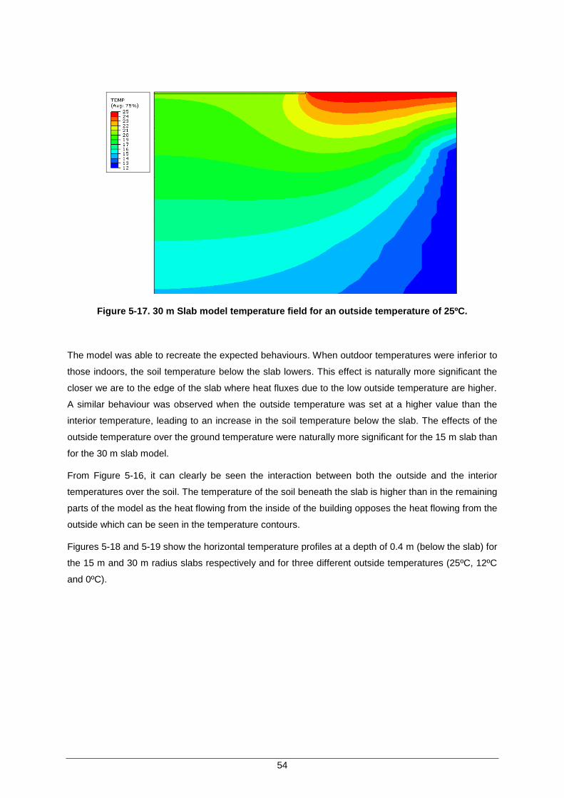
54
Figure 5-17. 30 m Slab model temperature field for an outside temperature of 25ºC.
The model was able to recreate the expected behaviours. When outdoor temperatures were inferior to
those indoors, the soil temperature below the slab lowers. This effect is naturally more significant the
closer we are to the edge of the slab where heat fluxes due to the low outside temperature are higher.
A similar behaviour was observed when the outside temperature was set at a higher value than the
interior temperature, leading to an increase in the soil temperature below the slab. The effects of the
outside temperature over the ground temperature were naturally more significant for the 15 m slab than
for the 30 m slab model.
From Figure 5-16, it can clearly be seen the interaction between both the outside and the interior
temperatures over the soil. The temperature of the soil beneath the slab is higher than in the remaining
parts of the model as the heat flowing from the inside of the building opposes the heat flowing from the
outside which can be seen in the temperature contours.
Figures 5-18 and 5-19 show the horizontal temperature profiles at a depth of 0.4 m (below the slab) for
the 15 m and 30 m radius slabs respectively and for three different outside temperatures (25ºC, 12ºC
and 0ºC).

55
Figure 5-18. Horizontal temperature profile below the 15m slab.
Figure 5-19. Horizontal temperature profile below the 30m slab.
For the 15 m slab case (Figure 5-18), results showed that for an outside temperature of 0ºC (winter
case) the ground surface temperature below the slab averaged 15.2ºC over the first 7.5 m which then
exponentially lowers as we get closer to its edge. When the outside temperature was set to 25ºC
(summer case) the same temperature value was 20.4ºC but increasing as we get closer to the slab’s
edge When the outside temperature was 12ºC an intermediate case between the two previously
described was verified.
Regarding the 30 m slab case (Figure 5-19), results showed for that for an outside temperature of 0ºC
(winter case) the ground surface temperature below the slab averaged 17.8ºC over the first 15 m which
then exponentially lowers as we get closer to its edge. When the outside temperature was set to 25ºC
(summer case) the same temperature value was 19.7ºC which increases as we get closer to the slab’s
edge.
0
5
10
15
20
25
30
0 10 20 30 40 50 60
Tem
per
atu
re (˚
C)
Distance from the slab centreline (m)
25˚C Outdoor Temp
0˚C Outdoor Temp
12ºC Outdoor Temp
0
5
10
15
20
25
30
0 10 20 30 40 50 60
Tem
per
atu
re (˚
C)
Distance from the slab centreline (m)
25˚C Outdoor Temp
0˚C Outdoor Temp
12˚C Outdoor Temp

56
According to the results illustrated in Figures 5-18 and 5-19, and taking into consideration that a steady
state analysis corresponds to an extreme case, we can conclude that the ground surface temperature
below the central zone of a building constructed according to current European regulations for thermal
insulation will be approximately that of the building’s interior decreased by 2 to 5ºC during winter or
increased by 0 to 1ºC during summer, depending on the dimensions of the building, the exact outdoor
temperature and proximity to the building edge. It can also be concluded that larger buildings will be
less affected in terms of temperature change beneath their ground floor slabs by the outside
temperature, when compared to smaller buildings since the soil itself acts as thermal insulation to heat
flowing from the building exterior.
Following these results and taking into consideration the model with the 30 m slab which is believed to
better represent the large building dimensions where thermal active piled foundations are usually
applied, a top temperature boundary condition of 18ºC will be used as the base case for the thermal-
mechanical model described in Section 6.2, the rather extreme values of 12ºC and 24ºC will also be
tested. This range of ground surface temperatures is believed to cover all the possible ground surface
temperatures that can be expected below the ground slab of any modern building. In effect, by simulating
the temperature below the ground slab with a constant magnitude, the modelling that follows assumes
that the pile is under the centre of a building of sufficient extent that heat flow from the building is
essentially one-dimensional and that seasonal effects can be neglected.
It is also important to mention that in reality, steady state conditions are unlikely to develop given the
seasonal nature of outdoor temperatures. Thomas & Rees (1999) present observations from a building
that was monitored which showed that the effect of seasonal temperature fluctuations on ground
temperatures are mainly seen only in the first few metres around the edges of the building.

57
Chapter 6
Thermal-Mechanical Analyses
6 Thermal-Mechanical Analyses
In this chapter, the results of a series of thermal-mechanical numerical analyses of a thermo-active pile
are presented and discussed.
58
6.1 Introduction
The thermal analysis performed in the previous section was of great importance to better understand
the problem of a heat exchanger pile from a purely thermal point of view. It was also helpful to determine
how certain modelling aspects such as the heating of the pile will affect the observed temperature fields
and if those results correspond to what is observed in reality.
In this section, the mechanical aspect of the problem was also taken into consideration, in order to
investigate how the thermal load affects the mechanical behaviour of the pile. Many of the conclusions
and findings of the previous thermal analysis will be taken into consideration in the development of the
thermal-mechanical model in this section. The impact of some thermal characteristics such as ground
surface temperature over the mechanical response of the pile will also be further investigated.
The following aspects of the thermo-active pile problem were the objective of study in this section:
The influence of the ground surface temperature;
The effect of differing relative values for the concrete and the soil coefficient of thermal
expansion;
The influence of the pile length and therefore the length to diameter ratio.
In order to investigate these aspects, a thermal-mechanical numerical model of the thermally-activated
pile problem was developed using the finite element software Abaqus. This model was used to run a
series of steady state thermal-mechanical analyses whose results are reported and discussed.
6.2 Numerical Model Implementation
The axisymmetric thermal model previously developed in Section 5.2.1 (Figure 5-2) was adopted but
was subject to some changes as the inclusion of the mechanical and thermal-mechanical effects added
a lot of complexity to the problem. These changes and the overall characteristics of the thermal-
mechanical model are discussed in the following sections.
6.2.1 Materials and material behaviour
Two materials were defined, concrete and soil. The same thermal properties used in the baseline
thermal analysis were adopted (Table 5-1) while the mechanical and thermal-mechanical properties are
indicated in Table 6-1.
The concrete linear coefficient of thermal expansion was assumed as 1.0E-5 m/m/K, according to data
published in Tatro (2006) who reports values of concrete CTE between 0.76E-5 m/m/K and 1.36E-5
m/m/K, depending on the aggregate type used in its production. Although a soil linear coefficient of

59
thermal expansion of 2E-5 m/m/K was adopted for the baseline analysis, values of 0.5E-5 m/m/K and
4E-5 m/m/K were also tested. As previously discussed in section 3.2.2, these three values can be related
to a lightly overconsolidated (OC), moderately OC and a heavily OC soil respectively. According to
Cekerevac and Laloui (2004), soil thermal expansion will increase with an increase in its OCR, and
highly OC soils can show a coefficient of thermal expansion several times higher than concrete.
Concrete was modelled as a purely elastic material while the soil was modelled as an elastic-perfectly
plastic material with a Tresca failure criteria: 1
2(𝜎1 − 𝜎2) ≤ 𝜏𝑢, where 𝜎1 and 𝜎2 are the principal stresses
and 𝜏𝑢 is the maximum shearing resistance of the soil. Plasticity was included in the soil model in order
to assess if the thermal load in combination with the design mechanical load were enough to induce soil
plasticity
Soil Concrete
Young Modulus, E (MPa) 30 30 000
Poisson's Coefficient, 0.3 0.3
Maximum shearing resistance, 𝝉u (kPa)
75 -
Linear coefficient of thermal expansion , α (m/m/K)
2E-5 1E-5
Table 6-1. Soil and concrete mechanical and thermal-mechanical properties.
6.2.2 Geometry, Mesh, Boundary Conditions and Initial Conditions
6.2.2.1 Geometry and Finite Element Mesh
The geometry of the thermal-mechanical model remains identical to that of the thermal model described
in Section 5.2.1. The pile in the baseline analysis has a diameter of 1 m and length of 30 m; piles of the
same diameter but with lengths of 15 m and 45 m were also tested as one of the parameter variations.
The bottom and side boundaries of the model were set at a distance of 90 m (3L) and 60 m (2L)
respectively. These boundary distances were proposed by Cruz Silva, 2012, who modelled a thermo-
active pile with the same geometry using the software ADINA. These boundary distances were also
tested using Abaqus and were found adequate to ensure the boundaries did not affect the pile response
significantly.
With the addition of mechanical behaviour to the model, the mesh previously developed for the
axisymmetric thermal model had to be reworked. In order to obtain adequate results, the thermal-
mechanical analysis demanded thinner elements than a purely thermal analysis, especially those
elements close to the pile which are responsible for dictating the development of its base and shear

60
resistance. Therefore, the mesh was refined, especially at the pile-soil interface and close to the pile. A
total of 3569 heat transfer four node elements were created for the baseline model (30 m long pile)
(Figure 6-1). The final mesh size was achieved through an iterative process, where the element size
was decreased up to a final state where any further decrease would not produce significant changes in
the result. Naturally, some mesh reworking was necessary when the pile length was changed to 15 m
and 45 m but its overall geometry and element density remained the same.
Figure 6-1. Mesh and boundary conditions of the thermal-mechanical model for the baseline
analysis.
6.2.2.2 Initial Conditions
Initial vertical stresses corresponding to both the weight of soil and concrete were applied to all the
elements of the model. The coefficient of lateral stress, K, was set to 1 meaning that the initial horizontal
stresses were considered equal to the vertical ones. All the elements of the model also have an initial
temperature of 15ºC. This is an idealization of what will happen in reality; as illustrated in Figure 2-1, the
temperature profile in the uppermost part of the soil profile will vary due to the actual climatic conditions
at the surface. For these analyses the simplification was made to reduce the number of variables being
considered.
6.2.2.3 Boundary Conditions
Following the results reported in Section 5.3, the thermal boundary condition on the top surface of the
model was set to a constant temperature of 18ºC for the baseline analysis. This was considered another
key parameter for the study and values of 12ºC and 24ºC were also considered as one of the parameter

61
variations.
The bottom and right hand side thermal boundary conditions of the model were set to a constant
temperature of 15ºC. While in the thermal model a value of 12ºC was used for these boundaries, it was
decided to increase it to 15ºC in the thermal-mechanical model so the results are somewhat comparable
to those reported by Bodas Freitas et al., 2013 who also used a value of 15ºC for these boundaries.
According to Figure 2-1, the soil temperature after a depth of 10 m to 15 m will be situated in between
12ºC to 15ºC in most European regions, so either of these values is acceptable.
Following the conclusions of Section 5.2.1, where full body heating and edge heating were found to
produce similar temperature fields at a steady state, and since the aim of the model was to recreate a
thermal pile whose absorber pipes are placed close to its edges (Figure 5-1 (a)), the heating of the pile
was simulated by applying an increase of 30ºC to all the elements making up the pile (full body heating).
While most of the analysis discussed in this thesis will only feature pile heating, a thermal cooling load
of -15ºC will also be tested. Since the heating thermal load will rise the pile temperature to 45ºC while
the ground surface will remain at 18ºC in the baseline analysis, a linear temperature decrease from 45ºC
to 18ºC at the ground surface next to the pile head was defined across a length of 0.5 m (Figure 6-1 in
orange). The same principle of pile-soil linear temperature transition was also applied when the ground
surface temperature was set to 12ºC and 24ºC. If this transition is not defined, calculation problems
were expected due to the definition of two very different temperature magnitudes at the same node.
Note that a temperature transition was not necessary to be defined at the upper right corner of the model
as the temperature difference between right BC and ground surface BC is much lower and any small
imprecision in the calculation of the temperature field in this zone will not affect the response of the pile.
Regarding the mechanical boundary conditions, the right boundary of the model is fixed in the horizontal
direction while the bottom boundary is fixed in both directions. The left boundary of the model
corresponds to the axis of symmetry.
Both thermal and mechanical boundary conditions are illustrated in Figure 6-1.
6.2.3 Pile-Soil Interface Behaviour
Initially, a perfectly rough pile-soil interface was assumed. However, this interface makes slippage
between the pile and the soil impossible as the interface of both these bodies is “tied” together.
It was then decided to simulate pile-soil interface behaviour by the addition of a layer of zero-thickness
interface elements whose tangential behaviour is modelled with an elastic-perfectly plastic constitutive
model (Figure 6-2). The interface elements mobilize shear resistance depending on the relative
displacement (slip) between the solid elements representing the soil and those representing the
concrete; in this case, reaching a maximum shearing resistance of 75 kPa for a total slip of 0.0015 m
(0.15%d).
The slip is measured as the vertical distance between nodes which initially, before any load is applied,
are connected (slip = zero). The amount of relative displacement required to fully mobilize the interface
resistance is not an intrinsic property and will depend on both the soil and the pile surface properties.

62
Figure 6-2. Interface elements constitutive model: total slip versus shear stress.
6.2.4 Model Validation
Unlike an elastic model, there are no analytical or numerical solutions available for the evaluation and
comparison of the bearing capacity of a pile in an elastic-plastic medium. In this study, model validation
was done through the analysis of the pile load-settlement curve in order to access if the model behaves
coherently and as expected.
The pile was loaded incrementally through the imposition of a settlement at its head and the predicted
load-settlement curve is plotted in Figure 6-3. The load was measured as the average axial stress at the
top four nodes of the pile, which constitute the pile head. The mobilized interface shear stress for four
different settlement values is plotted in Figure 6-4.
Two different pile behaviour phases can clearly be seen in Figure 6-3. Initially the pile has a stiffer
behaviour as it mobilizes mostly lateral resistance. During this initial phase the load-settlement curve is
approximately linear as both the soil and the interface are in an elastic state. At a settlement of about
18 mm, the pile lateral shearing resistance is fully mobilized which can be seen in Figure 6-3. Further
loading will then lead to a different behaviour as only base resistance remains to be mobilized and
therefore any load increment will lead to large settlement as the base resistance of the pile only accounts
for about 10% of the total pile resistance. This “two phase behaviour” is generally seen in real load tests
performed on piles placed in stiff clays, which work mainly through the mobilization of lateral shearing
resistance. At 400 mm settlement (40%d), the pile reached an ultimate load of 9.8 MPa (about 7.7 MN).
The pile-soil interface behaved as intended reaching a maximum shearing resistance of 75 kPa which
was obtained at a pile head settlement of about 18 mm. This means that for a settlement of 18mm the
soil nodes at the pile-soil interface averaged a vertical deformation of about 16.5 mm (91.7% of the
applied settlement) and the slip between the pile and soil was 1.5 mm, this being the maximum elastic
slip defined for the interface behaviour (see Figure 6-2).
Some perturbation of the interface shear stress profile (Figure 6-4) can be seen at the pile’s foot due to

63
soil movement and deformation in this zone.
The pile reached a total base resistance of 651 kN which given a 𝜏𝑢 value of 75 kPa results in a bearing
capacity factor, 𝑁𝑐, of 11 which is an acceptable value for a stiff clay.
Given these results, it can be concluded that the model is capable of modelling the mechanical
behaviour of a friction pile and produces sensible results.
Figure 6-3. Pile load-settlement curve.
Figure 6-4. Mobilized pile-soil interface shear stress.
0255075
100125150175200225250275300325350375400
0 2000 4000 6000 8000 10000
Sett
lem
ent
(mm
)
Axial Stress at the Pile Head (kPa)
0
5
10
15
20
25
30
0 15 30 45 60 75 90
Dep
th (
m)
Interface Shear Stress (kPa)
5mm Settlement
10mm Settlement
15mm Settlement
20mm Settlement
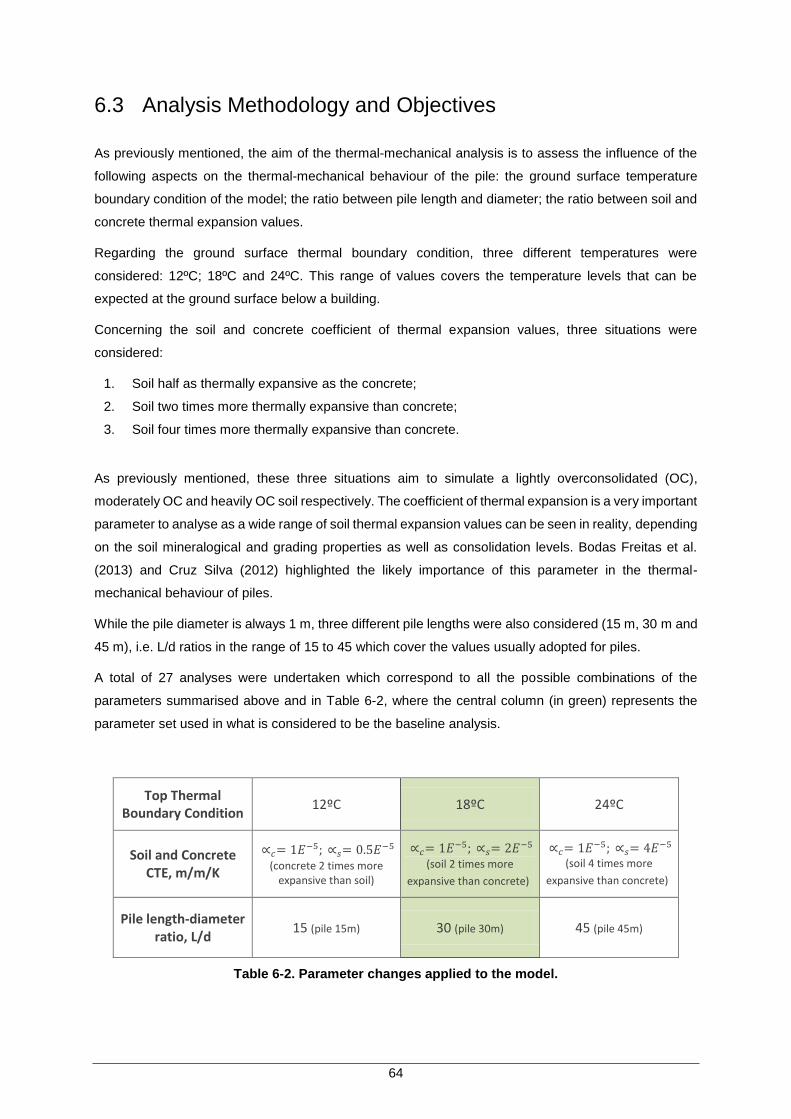
64
6.3 Analysis Methodology and Objectives
As previously mentioned, the aim of the thermal-mechanical analysis is to assess the influence of the
following aspects on the thermal-mechanical behaviour of the pile: the ground surface temperature
boundary condition of the model; the ratio between pile length and diameter; the ratio between soil and
concrete thermal expansion values.
Regarding the ground surface thermal boundary condition, three different temperatures were
considered: 12ºC; 18ºC and 24ºC. This range of values covers the temperature levels that can be
expected at the ground surface below a building.
Concerning the soil and concrete coefficient of thermal expansion values, three situations were
considered:
1. Soil half as thermally expansive as the concrete;
2. Soil two times more thermally expansive than concrete;
3. Soil four times more thermally expansive than concrete.
As previously mentioned, these three situations aim to simulate a lightly overconsolidated (OC),
moderately OC and heavily OC soil respectively. The coefficient of thermal expansion is a very important
parameter to analyse as a wide range of soil thermal expansion values can be seen in reality, depending
on the soil mineralogical and grading properties as well as consolidation levels. Bodas Freitas et al.
(2013) and Cruz Silva (2012) highlighted the likely importance of this parameter in the thermal-
mechanical behaviour of piles.
While the pile diameter is always 1 m, three different pile lengths were also considered (15 m, 30 m and
45 m), i.e. L/d ratios in the range of 15 to 45 which cover the values usually adopted for piles.
A total of 27 analyses were undertaken which correspond to all the possible combinations of the
parameters summarised above and in Table 6-2, where the central column (in green) represents the
parameter set used in what is considered to be the baseline analysis.
Top Thermal Boundary Condition
12ºC 18ºC 24ºC
Soil and Concrete CTE, m/m/K
∝𝑐= 1𝐸−5; ∝𝑠= 0.5𝐸−5 (concrete 2 times more
expansive than soil)
∝𝑐= 1𝐸−5; ∝𝑠= 2𝐸−5
(soil 2 times more
expansive than concrete)
∝𝑐= 1𝐸−5; ∝𝑠= 4𝐸−5 (soil 4 times more
expansive than concrete)
Pile length-diameter ratio, L/d
15 (pile 15m) 30 (pile 30m) 45 (pile 45m)
Table 6-2. Parameter changes applied to the model.

65
The thermal-mechanical analysis is run in three steps (geostatic, static and temperature-displacement)
and at a steady state. The three steps are performed in sequence where the results of one step become
the initial conditions of the following one. After the analysis is complete, not only the results of the final
step are available but also the results of the previous ones. Each of the three steps has the following
purpose:
1. Geostatic Step: The geostatic step is the initial step for most geotechnical studies performed in
Abaqus. In this step, the initial stresses corresponding to the weight of both the pile and the soil are
applied to the model. An initial temperature of 15ºC is also applied to all elements of the model. In
the geostatic step, Abaqus checks if the introduced stresses are in equilibrium and if all the elements
remain at an elastic state or not.
2. Static Step: In the static step the mechanical load is applied to the pile;
The mechanical load on the pile is applied as a uniform pressure at its head. A uniform pressure
load was preferred to a settlement load since the pile head must be able to move freely when the
thermal load is applied. Specifying a fixed displacement would not allow the pile head to freely
deform and would greatly affect the development of the thermally induced stresses.
The applied mechanical load value was calculated as the design load of the pile according to the
European regulation for geotechnical design (NP EN 1997-1). To obtain the design resistance, the
partial coefficients for resistance (𝛾𝑏 = 1.6; 𝛾𝑠 = 1.3) and the correlation factor (𝜉3 = 𝜉4 = 1.4) were
applied to both the shaft and the base resistances of the pile.
Regarding the base case (30 m pile), the calculated ultimate shaft resistance was 7069 kN and the
ultimate base resistance was 651 kN. By applying the appropriate partial factors from NP EN 1997-
1 to these values a pile design compression resistance of 4175 kN is obtained. Given the pile
diameter of 1 m, this translates into a uniform pressure of about 5.3 MPa. The same methodology
was applied in order to determine the mechanical load applied to both the 15 m and 45 m piles
which resulted in uniform pressures of 2.8 MPa and 7.8 MPa respectively.
3. Temperature-Displacement Step: In this last step the thermal load is applied to the pile.
The thermal load is applied as a “full body heat” (Figure 5-3 (a)), where the temperature of all the
pile elements was uniformly raised to 45ºC from the initial temperature of 15ºC (ΔT = +30ºC). While
an increase of 30ºC in the pile temperature is somewhat of an extreme value, field tests performed
in the past showed that it can happen in hot summers when the cooling demand is very high. This
value was chosen as we wanted to assess the maximum effect due to the thermal load that we can
expect in a thermally activated pile. The effect of a cooling thermal load (ΔT = -15ºC) was also
tested, however, in order not to excessively increase the number of analyses performed, the
parameter study discussed in Section 6.4.2 considers only a heating thermal load.

66
6.4 Results and Discussion
6.4.1 Baseline Analysis
As previously mentioned, the baseline analysis or base case corresponds to a 30 m long pile, an 18ºC
top thermal boundary condition and a soil with a coefficient of thermal expansion (2E-5 m/m/K) twice
that of the concrete (1E-5 m/m/K).
6.4.1.1 Baseline Analysis: Heating
Axial normal stresses in the pile, Figure 6-5 (a), and the pile-soil interface shear stresses, Figure 6-5
(b), show the effect of the mechanical load only, the thermal load only (temperature increase of 30°C)
and the combined effect of both these loads. Note that in Abaqus, positive axial stress values mean
tensile stress while negative values mean compressive stress.
Figure 6-5. Stresses in the pile and in the pile-soil interface.
Similar behaviours to those described in Section 4.1 were verified. The thermal load increased the axial
compressive load in the pile. The maximum thermally induced axial stress was 182.2 kPa and occurred
at a depth of 18.7 m which corresponds to the point where the strain restraint was highest. If the pile
was symmetrically restrained this point would be located at 15 m depth (middle of the pile) however, in
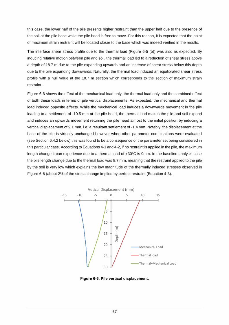
67
this case, the lower half of the pile presents higher restraint than the upper half due to the presence of
the soil at the pile base while the pile head is free to move. For this reason, it is expected that the point
of maximum strain restraint will be located closer to the base which was indeed verified in the results.
The interface shear stress profile due to the thermal load (Figure 6-5 (b)) was also as expected. By
inducing relative motion between pile and soil, the thermal load led to a reduction of shear stress above
a depth of 18.7 m due to the pile expanding upwards and an increase of shear stress below this depth
due to the pile expanding downwards. Naturally, the thermal load induced an equilibrated shear stress
profile with a null value at the 18.7 m section which corresponds to the section of maximum strain
restraint.
Figure 6-6 shows the effect of the mechanical load only, the thermal load only and the combined effect
of both these loads in terms of pile vertical displacements. As expected, the mechanical and thermal
load induced opposite effects. While the mechanical load induces a downwards movement in the pile
leading to a settlement of -10.5 mm at the pile head, the thermal load makes the pile and soil expand
and induces an upwards movement returning the pile head almost to the initial position by inducing a
vertical displacement of 9.1 mm, i.e. a resultant settlement of -1.4 mm. Notably, the displacement at the
base of the pile is virtually unchanged however when other parameter combinations were evaluated
(see Section 6.4.2 below) this was found to be a consequence of the parameter set being considered in
this particular case. According to Equations 4-1 and 4-2, if no restraint is applied in the pile, the maximum
length change it can experience due to a thermal load of +30ºC is 9mm. In the baseline analysis case
the pile length change due to the thermal load was 8.7 mm, meaning that the restraint applied to the pile
by the soil is very low which explains the low magnitude of the thermally induced stresses observed in
Figure 6-6 (about 2% of the stress change implied by perfect restraint (Equation 4-3).
Figure 6-6. Pile vertical displacement.
0
5
10
15
20
25
30
-15 -10 -5 0 5 10 15
Dep
th (
m)
Vetical Displacement (mm)
Mechanical Load
Thermal load
Thermal+Mechanical Load

68
While a “standard” thermal pile behaviour was observed for the baseline case, in reality the thermally
induced stresses are highly dependent on the relationship between pile and soil coefficients of thermal
expansion as well as the temperature field in the ground, as will be verified and discussed in the following
sections.
6.4.1.2 Baseline Analysis: Cooling
If thermal piles are used for heating a building instead of cooling, their temperature will reduce. In this
section the effects of a cooling thermal load (ΔT = -15ºC) are discussed and compared to the effects of
the heating thermal load previously analysed.
The effect of the heating and cooling thermal loads on the pile axial stress and pile-soil interface shear
stress are shown in Figure 6-7 (a) and Figure 6-7 (b) respectively.
Figure 6-7.Thermally induced stresses (heating and cooling thermal loads).
As expected, when the pile was cooled (ΔT=-15ºC) an opposite behaviour to the one previously
described for the heating thermal load (ΔT=+30ºC) was verified. As the pile is cooled it will tend to

69
contract, however, due to the restraint imposed in the pile by the soil, this contraction will be partially
prevented leading to the development of tensile stresses on the pile. For the case of ΔT=+30ºC, it can
be seen that the point of maximum restraint, which is the point of maximum axial stress, occurs at a
greater depth than for the case of ΔT=-15ºC, this phenomena is believed to be caused by a reduction of
the foot restraint. When the pile is cooled, the soil will also be cooled and tend to contract instead of
expand which is believed to lead to reduced restraint at the pile foot. Because the foot restraint reduces
the pile becomes more symmetrically restrained and the section of maximum strain restraint will get
closer to the middle of the pile.
While intuitively it would be expected that the thermally induced stresses in the pile would be proportional
to the thermal load, in fact, the results show that cooling apparently led to higher stress changes, even
though the temperature change was half that used for heating. This behaviour is related to the influence
of the ground surface temperature and to the fact that the soil is more thermally expansive than concrete.
In order to better explain these effects, a supplementary analysis was undertaken whereby only the
surface temperature was applied to the model (orange dashed line in Figure 6-7). In this supplementary
analysis, the change in axial stress was tensile with a value of about 180 kPa which is due to the warming
of the surface from the initial value of 15⁰C to 18⁰C and the associated soil expansion relative to that of
the pile. Now, when the change in axial stress due to the change in pile temperature is re-examined, the
change due to heating of +30⁰C is approximately twice that of cooling by -15⁰C. It is also interesting to
note that for the set of parameters used in this analysis, the thermal induced stresses in the pile due to
the sole increase in the ground surface temperature by 3ºC were of the same magnitude as those
induced by a pile heating of 30ºC. The effect of the relationship between soil and concrete thermal
expansion values and the ground surface temperature over the thermally induced stresses in the pile is
further studied in Sections 6.4.2.1 and 6.4.2.2 respectively.
Note that the effect of the surface temperature has not been decoupled as it was considered that the
two forms of thermal loading are likely to occur more-or-less simultaneously, i.e. the building will come
to some long-term temperature equilibrium at the same time that the foundation piles are being used for
heating and cooling. It is interesting to note however that the effect on the pile response due to the
surface temperature alone is of a similar magnitude to that seen for the temperature changes applied to
the pile.
In order to not excessively increase the number of numerical analyses performed in the parameter study
presented in Section 6.4.2, the pile was only subjected to heating (ΔT = +30ºC) and cooling was not
considered.
6.4.2 Parameter Study
6.4.2.1 Soil and concrete coefficient of thermal expansion
Figure 6-8 (a) and (b) illustrate the axial stress and interface shear stress changes developed due to
the heating thermal load (ΔT = +30ºC) for the three combinations of soil and concrete thermal expansion

70
values previously detailed. All the remaining model parameters remained the same as in the baseline
analysis.
These figures clearly show the influence of the relative values of the concrete and soil thermal expansion
coefficients with respect to the changes in axial stress and shear stress during thermal loading,
confirming the results reported by Bodas Freitas et al, (2013). In fact, this relationship is responsible for
dictating not only the magnitude of the thermally induced stresses but also their direction.
When soil is half as thermally expansive as concrete (blue lines in Figure 6-8) similar behaviour to what
was previously described in the heating baseline analysis (Section 6.4.1.1) was observed, however the
magnitude of the developed stresses was considerably higher. This happens because the soil has a
lower tendency to expand; the relative movement between the soil and the pile is greater and therefore
the change in shear stress in the interface is larger. This results is greater restraint of the pile and
consequently, the development of larger magnitude thermally induced axial stress.
When the soil is four times more expansive than concrete, the pile goes into tension. In this case,
because the soil is considerably more thermally expansive than concrete, it will expand more than the
pile, which leads to the development of tensile stresses.
When the soil is two times more expansive than concrete (the base case), we are in a situation in
between the two previously described. As the soil is more expansive than the concrete, tensile stresses
would be expected in response to heating, this doesn’t happen because the pile is at a higher
temperature than the soil. For the combination of parameters used in this case, the resultant effect is
for the pile to expand slightly more than the soil does and the two effects, soil and pile expansion, end
up opposing each other and resulting in low magnitude thermally induced compressive stresses.

71
Figure 6-8. Thermally induced stresses for three cases of soil and concrete thermal expansion
values.
The change in pile vertical displacements due to the thermal load is plotted in Figure 6-9. It can be seen
that as we increase the coefficient of thermal expansion of the soil, the more the pile moves upwards
due to the thermal load. This is due to the added increase in volume the soil experiences which “pushes”
the pile upwards. Comparing the results from the cases when the soil is 2 times and 4 times more
expansive than concrete, it can also be seen that the pile is also slightly stretched due to the high tensile
stresses the soil imposes over it. In fact, according to Equations 4-1 and 4-2, if the effect of soil
expansion is ignored, the maximum length change the pile can experience due to a thermal load of
+30ºC is 9mm, while for the case when the soil was 4 times more thermally expansive than concrete,
this length change was 9.4mm, proving the stretching effect the soil has over the pile.
Figure 6-9. Thermally induced vertical displacements in the pile for three cases of soil and
concrete thermal expansion values.
6.4.2.2 Ground Surface Temperature
Figures 6-10 (a) and (b) illustrate the thermally induced stresses in the pile and interface for three
different ground surface temperature boundary conditions: 12ºC; 18ºC (base case) and 24ºC. These
boundary conditions aim to recreate the range of ground surface temperature that can be expected
below a building’s ground slab. Naturally, these boundary conditions will have a great effect over the
soil temperature field especially in the upper part of the model and therefore affect how much it will try
to expand or contract, and how it will interact with the pile.
Because all the elements forming the pile are heated to a constant temperature of 45ºC, a change in
the ground surface thermal boundary condition will only affect the temperature of the soil and therefore

72
how much it expands or contracts. Besides the ground surface temperature, all the other model
parameters remained the same as in the baseline analysis.
Figures 6-10 (a) and (b) show a clear influence of ground surface temperature over both the magnitude
and direction of the thermally induced stresses in the pile. In comparison to the base case (red line), an
increase in ground surface temperature changed the thermally induced axial stresses from compressive
to tensile and the direction of the interface shear stresses. To understand this behaviour it is important
to remember that in this analysis, the soil is twice as thermally expansive as the pile; therefore, any
increase in temperature will lead to a significant expansion of the soil. By increasing the ground surface
temperature, we also increase the average temperature of the soil mass beneath it, which will lead to
expansion and the development of tensile stresses in the pile, as the soil will expand more than the pile.
The opposite phenomenon happens when we decrease the ground surface temperature. Reducing the
temperature of the soil below the initial state will lead to contraction and the development of larger
compressive stresses in the pile. In this case, even though the pile is less expansive than the soil,
because it is subjected to considerably higher temperatures it will still show a tendency to expand more
than the soil which will lead to compressive thermally induced stresses.
Figure 6-10. Thermally induced stresses for three different ground surface temperatures.
The change in pile vertical displacements due to the ground surface temperature is plotted in Figure
6-11. From this figure it can be seen that as we increase the ground surface temperature the more pile
moves upwards. This behaviour is due to the added soil expansion, especially at the upper part of the
model, caused by an increase in the ground surface temperature. As the soil tends to expand against
the pile, it will induce tension in the pile and lift it. For instance, for the case of a 24ºC thermal BC, the

73
pile total length change due to the thermal load was 9.1mm, while Equations 4-1 and 4-2, which don’t
take into consideration the effect of the soil expansion, predict a maximum pile length change of 9mm.
Figure 6-11. Thermally induced vertical displacements for three different ground surface
temperatures.
6.4.2.3 Pile diameter-length ratio
Figures 6-12 (a) and (b) illustrate the thermally induced stresses in the pile and pile-soil interface for
three different pile lengths: 15 m; 30 m (base case) and 45 m. The pile diameter is 1 m for the three
cases, the soil is two times more expansive than concrete, and all the remaining model parameters are
those of the baseline analysis.
While a change in the pile length didn’t induce any behaviour changes in the pile, i.e. the resultant effect
was compressive thermally induced stresses in all three cases, the magnitude of the developed stresses
was clearly affected by this change as the longer the pile (larger the ratio, L/d), the larger were the
mobilized pile axial normal stresses and the pile-soil interface shear stresses (Figures 6-12(a) and (b)).
Two phenomena are believed to be the cause of this increase in thermally induced stresses:
1. The main cause derives from the fact that the longer the pile is, the more it will expand or contract
when subjected to a temperature change and therefore the higher the shear stresses mobilized at
the pile-soil interface will be. This mobilization of shear stress will induce strain restraint in the pile
and thermally induced stresses are directly proportional to the amount of strain restraint (Equation
4-3). If the soil and the interface remain elastic, the increase in thermally induced stress due to the
increase in strain restraint with pile length is believed to be a linear effect.
2. A second cause of this behaviour, while perhaps less important than that described above, is the
variation of the soil temperature field with depth. In fact, in the baseline analysis, the top boundary
0
5
10
15
20
25
30
-5 0 5 10 15
Dep
th (
m)
Vetical Displacement (mm)
12ºC Thermal BC
18ºC Thermal BC (base case)
24ºC Thermal BC

74
of the model is kept at 18ºC while the bottom at 15ºC, This means that temperature field around the
15 m pile will be generally warmer than that of say the 45 m pile and therefore, in the former case,
the effect of the temperature change in the pile on the soil temperature will be less. If the temperature
change is less, then the relative movement on the pile-soil interface will be smaller leading to lower
changes in shear stress and pile restraint.
Figure 6-12. Thermally induced stresses for three different pile lengths.
6.4.2.4 Result summary and interaction between the studied parameters
Figures 6-13, 6-14 and 6-15 illustrate the maximum thermally induced axial load in the pile as a function
of the ground surface temperature for the three pile lengths and the three ratios of soil to concrete
coefficients of thermal expansion previously considered. Each figure corresponds to a fixed pile length
(15 m, 30 m and 45 m). As noted previously, in these figures, positive axial load values represent tensile
stress and negative values, compressive stress.
These figures show a strong influence of the ground surface temperature over the thermally induced
axial load on the pile, as previously assessed in Section 6.4.2.2. A clear connection between this
influence and the relationship between soil and concrete coefficients of thermal expansion can be seen.
In fact, the effect of the ground surface temperature will greatly increase with an increase of the
coefficient of thermal expansion of the soil and the thermally induced stresses will become increasingly
tensile. This behaviour can be explained as the higher the soil coefficient of thermal expansion is, the

75
more it will tend to expand relative to the pile for the same temperature change and therefore the more
tensile the stresses it will induce.
As discussed in Section 6.4.2.3, the longer the pile, the higher the thermally induced stresses will be
due to the increase in the pile restraint.
Figure 6-13. Maximum thermally induced axial stress in the pile as a function of the ground
surface temperature (15m pile).
Figure 6-14. Maximum thermally induced axial stress in the pile as a function of the ground
surface temperature (30m pile).

76
Figure 6-15. Maximum thermally induced axial stress in the pile as a function of the ground
surface temperature (45m pile).
The same data set is re-visualised in Figures 6-16, 6-17 and 6-18 however in this case each figure
corresponds to a fixed value of the ratio between the soil and concrete coefficient of thermal expansion.
Once again, positive axial load values represent tensile stress while negative values compressive stress.
When the soil is less thermally expansive than concrete (Figure 6-16), the ground surface temperature
has a minimal impact over the thermally induced stresses in a pile of a particular length, and the stress
changes are always compressive. Since in this case the concrete is more expansive than soil and since
the pile will be at a higher temperature than the soil independently of the ground surface temperature
adopted, it is natural that a variation of the ground surface temperature won’t induce significant change
as the pile will always expand considerably more than the soil. However, as we increase the soil’
coefficient of thermal expansion (Figures 6-17 and 6-18), the ground surface temperature becomes
increasingly important and thermally induced stresses become increasingly tensile.
When the soil is two times more expansive than the concrete (Figure 6-17), this complex and interesting
interaction between pile and soil can clearly be seen. In this case, even though the soil coefficient of
thermal expansion is higher than the concrete, for the low ground surface temperatures we still verify
compressive stresses because the pile temperature is considerably higher than that of the soil, and the
pile will expand more than the soil does. However, as we increase the ground surface temperature and
therefore the soil temperature, this behaviour starts to reverse and the compressive stresses start
reducing and eventually, the thermally induced stresses on the pile become tensile. The surface
temperature at which this transition occurs can be seen to vary with the pile length.

77
Figure 6-16. Maximum thermally induced axial stress in the pile as a function of the ground
surface temperature (soil half as thermally expansive as concrete).
Figure 6-17. Maximum thermally induced axial stress in the pile as a function of the ground
surface temperature (soil two times more thermally expansive than concrete).
When the soil is four times more expansive than the concrete (Figure 6-18), the soil tendency to expand
will always surpass that of the concrete if the ground surface temperature is 13ºC or higher. In this case,
thermally induced compressive stresses will only develop in the pile for very low ground surface
temperatures (<12ºC), which is when the pile will start expanding more than the soil.

78
Figure 6-18. Maximum thermally induced axial stress in the pile as a function of the ground
surface temperature (soil four times more thermally expansive than concrete).
Figure 6-19 shows the same data set redrawn yet again with the thermally induced axial stresses
expressed as a function of the ratio between soil and concrete coefficient of thermal expansion (αsoil and
αconc) and for a pile length of 30 m. Once again, the significant influence of the ground surface
temperature over the thermally developed stresses is clearly seen. However and as expected, these
lines converge to the same value for the case of a soil with a coefficient of thermal expansion of zero.
In fact, when the soil coefficient of thermal expansion is zero, a change of the ground surface
temperature won’t produce any effect because the soil becomes “immune” in terms of volumetric
changes to any thermal load and the pile temperature is unaffected by the ground surface temperature
as it was modelled to heat uniformly to 45ºC and to remain at this temperature.
When the ratio of soil to concrete coefficient of thermal expansion is equal to zero, the maximum
thermally induced axial stress in the 30 m pile in Figure 6-22 is about 900 kN; in the 15 m long pile it
was about 300 kN and the 45 m pile, 1600 kN. In relation to the length of the pile, the thermally induced
stress in the pile when the ratio of soil to concrete coefficient of thermal expansion is equal to zero, is
approximately linear.
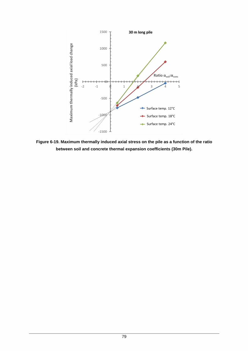
79
Figure 6-19. Maximum thermally induced axial stress on the pile as a function of the ratio
between soil and concrete thermal expansion coefficients (30m Pile).

80

81
Chapter 7
Conclusions
7 Conclusions
The current thesis intended to analyse in a systematic way the thermal-mechanical behaviour of thermo-
active piles. Thermal and thermal-mechanical numerical analyses were conducted whose main results
and conclusions are summarized in this chapter.

82
7.1 Conclusions and Results Summary
Thermal and thermal-mechanical numerical analyses of a thermally activated pile were performed in
this thesis using the finite element software Abaqus. It is believed that these analyses produced
important and interesting results which will definitely contribute to improving our current knowledge
regarding the thermal-mechanical behaviour of energy foundations. Some of the reported findings may
also help in the future development of numerical models as a number of simulation hypotheses and
simplifications were studied in order to investigate their legitimacy.
Regarding the thermal analysis, the most significant results were the following:
At a steady state, full body and edge heating produced similar temperature fields; however those
obtained from centreline heating showed considerably lower temperatures especially at the pile-
soil interface (Figure 5-6). Consequently, if the energy pile being simulated has its heat
exchange pipes placed close to the centreline, full body heating or edge heating are not
appropriate and centreline heating should be adopted.
The pipe layout and ring heating produced similar temperature fields at a steady state; however
a transient analysis showed that the temperature fields differed considerably during the first
weeks of heating (Figure 5-14). If a transient analysis of an energy pile is required, it is
recommended that the pipe layout is modelled.
The ground surface temperature below the central zone of a building constructed according to
current European regulations for thermal insulation will be approximately that of the building’s
interior decreased by 2 to 5ºC during winter or increased by 0 to 1ºC during summer, depending
on the dimensions of the building, the exact outdoor temperature and proximity to the building
edge. As thermally activated piles are generally placed beneath the building, these results can
be used to determine an approximate value for the ground surface temperature which can be
applied to a numerical simulation.
Regarding the thermal-mechanical analysis, the most significant results were the following:
The relative values of the coefficient of thermal expansion for the soil and the concrete play a
key role in dictating the direction and the magnitudes of the developed stresses in a pile
subjected to thermal loading. Results showed that even for the same thermal load, this ratio can
dictate if the thermally induced stresses in the pile will be compressive or tensile.
If the soil is more thermally expansive than concrete, the ground surface temperature has a very
important influence over the thermally induced stresses developed in the pile. This effect was
however considerably less significant if the concrete is more expansive than soil. It is therefore
83
recommended that numerical simulations of energy piles pay close attention to the correct
definition of the ground surface temperature.
For the same pile diameter, the longer the pile, the larger the thermally induced stresses will be.
This phenomenon is believed to be caused mainly by the increased shear stress mobilized at
the pile-soil interface which increases restraint on the pile. To a lesser extent, the variation of
the ground temperature with depth may also affect the development of thermally induced
stresses for piles with different lengths, especially when soil presents a higher thermal
expansion coefficient than concrete.
7.2 Future Developments
Following the thermal mechanical analysis performed in this thesis, it was determined that the
relationship between the coefficient of thermal expansion of concrete and soil has a vital influence over
the observed thermal-mechanical behaviour of an energy pile. While a homogenous soil was admitted
in this study, in reality, soils are generally heterogeneous and different soil layers, whose thermal-
mechanical properties are not the same, can usually be identified in most construction sites. Therefore,
it would be important to run a similar study as the one presented in this thesis but where two or more
different soil layers are modelled and whose coefficients of thermal expansion, in particular, vary. This
change is expected to produce considerable changes in the thermally induced stresses in the pile which
will be the result of the complex interaction between the soil layers and the pile. The understanding of
this interaction would be an important step in achieving a complete understanding of the effects of the
thermal load over a foundation pile.
While an isolated thermo-active pile was considered in this thesis, in reality, a number of piles are
required to effectively heat/cool a building and therefore these piles are usually placed in groups. The
addition of one or more piles to the model will lead to changes in its temperature field which, as
discussed in this thesis, will lead to significant stress changes in the piles, especially if the soil is more
thermally expansive than concrete. It would be of great interest to assess how significant these stress
changes would be in order to better understand if the thermo-active pile problem can be studied from a
single pile perspective or if the modelling of the pile group is required.
Other possible developments to the analyses discussed in this thesis are:
Studying the behaviour of the thermo-active pile through time by adopting a cyclic thermal load,
according to the heating/cooling seasons, instead of a constant temperature increase/decrease.
This study will also require a change from a steady state to a transient thermal-mechanical
analysis and the development of a 3D pile model with a pipe layout;
Addressing the influence of the soil and pile-soil interface stiffness to the observed thermal-
mechanical response of the pile.

84
85
References
References
Amis, T. (2011) Energy foundation in the UK. UK Ground Source Heat Pump Association conference,
Ground Source Live, Petersborough (http://www.gshp.org.uk/Ground_Source_Live_2011.html).
ASHRAE (2009). ASHRAE Handbook—Fundamentals (SI), American Society of Heating, Refrigerating
and Air-Conditioning.
Bodas Freitas, T. M., Cruz Silva, F. and Bourne-Webb, P.J. (2013). The response of energy foundations
under thermo-mechanical loading, Accepted for publication in the Proc. 18th ICSMFE, Paris, 4 pages.
Bourne-Webb, P. J., Amatya, B., Soga, K., Amis, T., Davidson, T. & Payne, P. (2009) Energy pile test
at Lambeth College, London: geotechnical and thermodynamic aspects of pile response to heat cycles,
Geotechnique, 59 (3), 237-248.
Bourne-Webb, P., Amatya, B. & Soga, K. (2013) A framework for understanding energy pile behaviour,.
Proceedings of the Institution of Civil Engineers Geotechnical Engineering.
Bourne-Webb, P. (2014) A framework for understanding energy pile behaviour. Presented to British
Geotechnical Association evening meeting.
Brandl, H. (2006) Energy foundations and other thermo active ground structures, Geotechnique, 56 (2),
81 – 122.
Baldi G, Hueckel T, Pelegrini R. Thermal volume changes of the mineral-water system in low-porosity
clay soils.Canadian Geotechnical Journal 1988; 25:807–825.
Cekerevac C and Laloui L (2004) Experimental study of thermal effects on the mechanical behaviour of
a clay. International Journal for Numerical and Analytical Methods in Geomechanics 28(3): 209–228.
Cruz Silva F. 2012. Load-displacement behaviour of thermo-active piles. MSc Thesis, Instituto Superior
Técnico, Lisboa, Portugal, 105 pages.
Di Donna, A., Dupray, F., & Laloui, L. (2013). Effect of thermo-plasticity of soils on the design of energy
piles, Proc. European Geothermal Conference, EGC 2013, Pisa, Italy, 1-8.
Eurima, 2011. U-values in Europe. European Insulation Manufacturer Association
(http://www.eurima.org/index.php?page=u-values-in-europe).
Farouki, O. T. (1986) Thermal Properties of Soils, Series on Rock and Soil Mechanics Volume 11, Trans
Tech Publications, Germany.
Hiraiwa, Y. & Kasubuchi, Y. (2000) Temperature dependence of thermal conductivity of soil over a wide
range of temperatures (5-75oC), European Journal of Soil Science, 51, 211-218.

86
Laloui, L., Nuth, M. & Vulliet, L. (2006) Experimental and numerical investigations of the behaviour of
heat exchanger pile, International Journal for Numerical and Analytical Methods in Geomechanics, 30,
763-781.
Loveridge, F. (2012). The Thermal Performance of Foundation Piles used as Heat Exchangers in
Ground Energy Systems. PhD thesis. University of Southampton, Southampton, United Kingdom, 179
pages.
Neville, A.M., 1995. Properties of concrete, 4th edition. Longman, London.
Perry, J., Loveridge, F. & Bourne-Webb. P. (2011). Ground Sourced Energy, Evolution, Winter 2011,
20-23.
Powrie, W.,& Loveridge, F. (2013). Pile heat exchangers: thermal behaviour and interactions.
Proceedings of the ICE – Geotechnical Engineering, 166(2), 178-196.
Rees, S. W., Adjali, M. H., Zhou, Z., Davies, M. & Thomas, H. R. (2000) Ground heat transfer effects on
thermal performance of earth contact structures, Renewable and Sustainable Energy Reviews, 4, 213-
265.
Rees, S. W., & Thomas, H. R. (2009). Measured and simulated heat transfer to foundation soils.
Géotechnique, 59(4), 365–375.
Surayatriyastuti, M., Mroueh, H, and Burlon, S. (2013). Numerical analysis of a thermo-active pile under
cyclic thermal loads, Proc. European Geothermal Conference, EGC 2013, Pisa, Italy, 1-8.
Sultan, N., Delage, P. & Cui, Y. J. (2002). Temperature effects on the volume change behaviour of
Boom clay. Engineering Geology 64, 135-145.
Tatro S.B., (2006). Thermal properties, in – STP169D Significance of tests and properties of concrete
and concrete-making materials, Lamond and Pielert eds., ASTM International, USA, p. 226-237.
Thomas H. R., Rees S. W. (1999). The thermal performance of ground floor slabs – a full scale in-situ
experiment. Building and Environment 34 (1999). Pp 139 – 164.