thermal models in emeraude a sensitivity study
TRANSCRIPT

Emeraude thermal models: a sensitivity study © KAPPA 1988‐2011 Emeraude 2.60 ‐ 1/23
Thermal models in Emeraude
A Sensitivity Study
This document aims at helping the Emeraude user to understand the differences between the Segmented Model and the Energy Model, facilitating the selection of one or the other when interpreting a PL job. This document provides a brief theoretical description of each model, followed by a sensitivity study exhibiting the influence of different parameters (geophysical, geometrical or PVT) on these models.
Finally, time dependency for both models is compared and the Energy model is checked versus a real multiphase case exhibiting the possible importance of annular free convection.

Emeraude thermal models: a sensitivity study © KAPPA 1988‐2011 Emeraude 2.60 ‐ 2/23
Table of Contents I. Physical properties of some common materials ............................................................................. 3
II. Segmented Model ........................................................................................................................... 4
I.a. Theory ...................................................................................................................................... 4
I.a.1 Within inflow zones ............................................................................................................. 4
I.a.2 Between inflow zones ......................................................................................................... 5
I.b. Sensitivity analysis ................................................................................................................... 5
I.b.1 dP Joule‐Thomson ............................................................................................................... 6
I.b.2 Heat loss coefficient ............................................................................................................ 7
I.b.3 Parameters acting on the HLC ............................................................................................. 7
I.b.4 Fluid heat capacity ............................................................................................................... 9
I.b.5 Fluid thermal conductivity ................................................................................................. 10
I.b.6 Sensitivity summary .......................................................................................................... 10
III. Energy model ............................................................................................................................. 11
II.a. Theory .................................................................................................................................... 11
II.a.1 Mass balance ..................................................................................................................... 11
II.a.2 Energy balance .................................................................................................................. 11
II.a.3 Heat loss coefficient calculation ........................................................................................ 13
II.a.4 Pressure drop calculation .................................................................................................. 14
II.b. Sensitivity analysis ................................................................................................................. 15
II.b.1 Reservoir thermal conductivity ..................................................................................... 15
II.b.2 Reservoir radius ............................................................................................................. 15
II.b.3 Fluid heat capacity ......................................................................................................... 16
II.b.4 Heat loss coefficient ...................................................................................................... 16
II.b.5 Parameters acting on the HLC ....................................................................................... 18
II.b.6 Parameters acting on heat transport from/to the reservoir ......................................... 19
II.b.7 Sensitivity summary ...................................................................................................... 21
IV. Influence of other parameters .................................................................................................. 22
III.a. Time dependency .................................................................................................................. 22
III.b. Annular free convection .................................................................................................... 22
Emeraude thermal models: a sensitivity study © KAPPA 1988‐2011 Emeraude 2.60 ‐ 3/23
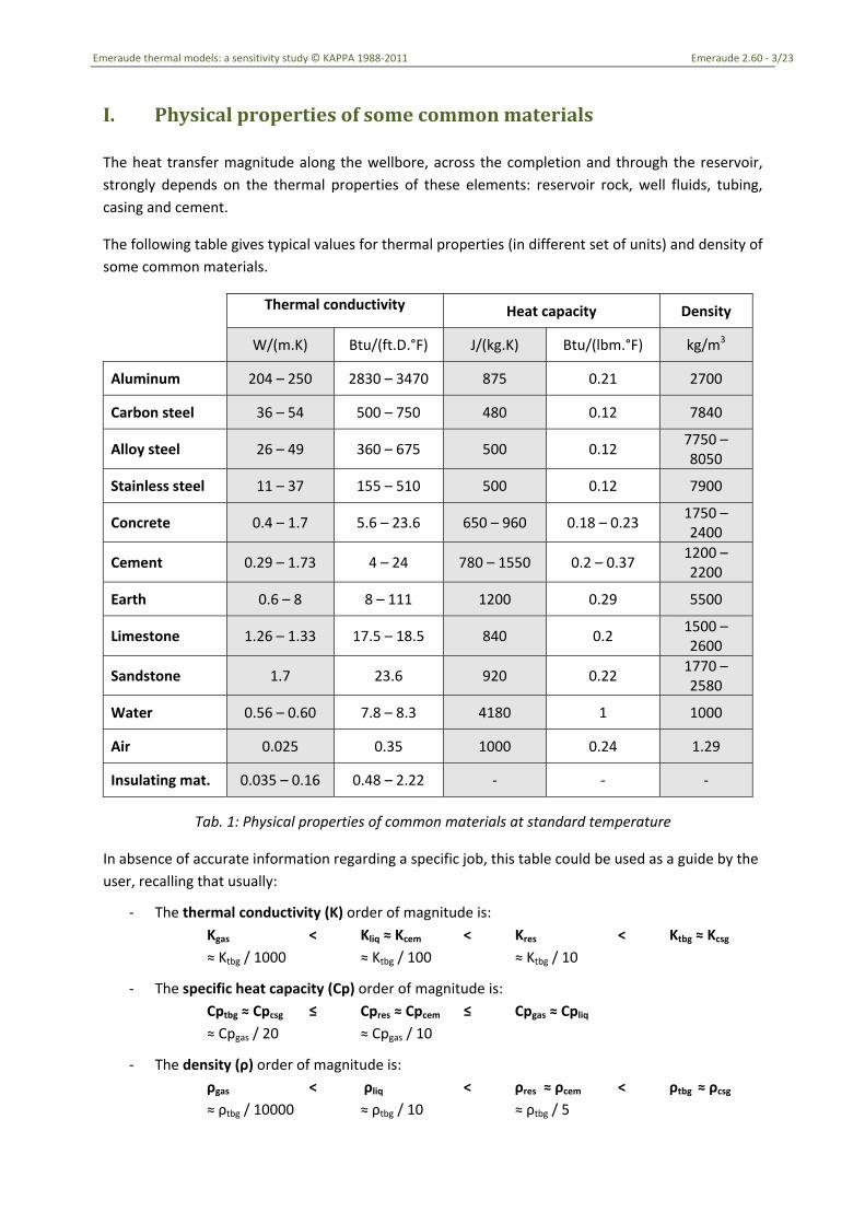
I. Physical properties of some common materials The heat transfer magnitude along the wellbore, across the completion and through the reservoir, strongly depends on the thermal properties of these elements: reservoir rock, well fluids, tubing, casing and cement.
The following table gives typical values for thermal properties (in different set of units) and density of some common materials.
Thermal conductivity Heat capacity Density
W/(m.K) Btu/(ft.D.°F) J/(kg.K) Btu/(lbm.°F) kg/m3
Aluminum 204 – 250 2830 – 3470 875 0.21 2700
Carbon steel 36 – 54 500 – 750 480 0.12 7840
Alloy steel 26 – 49 360 – 675 500 0.12 7750 – 8050
Stainless steel 11 – 37 155 – 510 500 0.12 7900
Concrete 0.4 – 1.7 5.6 – 23.6 650 – 960 0.18 – 0.23 1750 – 2400
Cement 0.29 – 1.73 4 – 24 780 – 1550 0.2 – 0.37 1200 – 2200
Earth 0.6 – 8 8 – 111 1200 0.29 5500
Limestone 1.26 – 1.33 17.5 – 18.5 840 0.2 1500 – 2600
Sandstone 1.7 23.6 920 0.22 1770 – 2580
Water 0.56 – 0.60 7.8 – 8.3 4180 1 1000
Air 0.025 0.35 1000 0.24 1.29
Insulating mat. 0.035 – 0.16 0.48 – 2.22 ‐ ‐ ‐
Tab. 1: Physical properties of common materials at standard temperature
In absence of accurate information regarding a specific job, this table could be used as a guide by the user, recalling that usually:
‐ The thermal conductivity (K) order of magnitude is: Kgas < Kliq ≈ Kcem < Kres < Ktbg ≈ Kcsg ≈ Ktbg / 1000 ≈ Ktbg / 100 ≈ Ktbg / 10
‐ The specific heat capacity (Cp) order of magnitude is: Cptbg ≈ Cpcsg ≤ Cpres ≈ Cpcem ≤ Cpgas ≈ Cpliq ≈ Cpgas / 20 ≈ Cpgas / 10
‐ The density (ρ) order of magnitude is: ρgas < ρliq < ρres ≈ ρcem < ρtbg ≈ ρcsg ≈ ρtbg / 10000 ≈ ρtbg / 10 ≈ ρtbg / 5

Emeraude thermal models: a sensitivity study © KAPPA 1988‐2011 Emeraude 2.60 ‐ 4/23
II. Segmented Model
II.a. Theory Two distinct models are used, whether the simulation is made within, or outside inflow zones.
II.a.1 Within inflow zones The temperature is calculated from enthalpy balance.
The enthalpy of the fluid at the bottom of the inflow zone is calculated as:
Tb, the bottom temperature, is read directly from the reference temperature log. The Cp’s are the heat capacities of the various fluids, defined in the PVT model. The enthalpy at the top of the inflow zone is given by:
It is assumed that the geothermal temperature profile is given. The incoming fluids are supposed to enter at a temperature equal to the geothermal temperature at the mid‐point of the inflow zone, Tgeo. For the gas, the entry temperature is corrected for Joule‐Thomson. Joule‐Thomson: For the gas, an isenthalpic process is assumed, leading to:
Enthalpy balance between the top and bottom of the inflow zone gives:
Therefore:
Note that this equation does hold only if all the contributions are positive. Extensions are made in other situations.
Emeraude thermal models: a sensitivity study © KAPPA 1988‐2011 Emeraude 2.60 ‐ 5/23
II.a.2 Between inflow zones With Reference to the SPE Reprint Series No 19, and more specifically the paper "Use of Temperature Log For Determining Flow Rates in Producing Wells", by Curtis & Witterholt, the temperature above a fluid entry zone is given by:
This equation was introduced by Ramey. Tf = wellbore temperature TGe = geothermal temperature at depth of fluid entry gG = geothermal gradient z = distance from fluid entry measured upwards Tfe = wellbore temperature at depth of fluid entry A = relaxation distance
Under certain assumptions, the relaxation distance A can be expressed as:
In Emeraude, the user is asked to input a Heat loss coefficient equal to the inverse of:
Heat loss coefficient: it can be expressed using the formation heat conductivity, and diffusivity. The time function, f(t), is given by Ramey and could then be calculated knowing the production time. Another approach allows calculating this coefficient directly from the log, if the surface rates are known. Both approaches are available in Emeraude, but note that in the latter case, the calculation will be done automatically when reaching Zone Rates the first time. Also, the heat loss coefficient can be included in the regression when matching surface conditions (only if kept constant over the entire log interval). II.b. Sensitivity analysis As described above, two parameters are governing the Segmented Model: ‐ Delta‐P Joule‐Thomson (dPJT): applies on the inflow zones to quantify a temperature change
due to a pressure change. However, the equation describing the heat transfer from the reservoir to the well neglects several phenomena such as: thermal conduction, kinetic and potential energy changes. In order to properly consider them, the dP value must be corrected for these effects: as it corresponds to a non linear equilibrium, the correction cannot be simply evaluated a priori, but must be obtained by a trial and error procedure.
‐ Heat loss coefficient (HLC): applies between the inflow zones and accounts for the heat transfer by conduction in the reservoir and across the completion.
The following figures show the influence of dPJT and HLC on the Segmented Model predictions, as well as the influence of other parameters on the HLC. The results have been obtained by running several cases on a single phase gas producer (methane), with three contributing zones (this corresponds to Emeraude Guided Session B10).

Emeraude thermal models: a sensitivity study © KAPPA 1988‐2011 Emeraude 2.60 ‐ 6/23
Fig. 1: Temperature profiles for different dPJT
Fig. 2: Temperature profiles for different HLC
II.b.1 dP Joule‐Thomson Fig. 1 above shows the thermal profiles predicted by the Segmented Model when the dPJT (pressure drop) increases from 0 psi ( ) to 100 psi ( ), the zone contributions being unchanged from one case to another. The calculated temperature profiles range from 163.8°F to 166.6°F.
Starting from the geothermal ( ) below the lower inflow (white zones visible on the zones track), the cooling over this inflow increases with dPJT. Then, between the bottom inflow and the middle one, the Segmented Model restarts calculating the temperature from the geothermal with the same HLC for all cases, and independently of the temperature found at the top of the inflow below: all curves are identical. When reaching the middle inflow, the dPJT induces a cooling as expected, although possibly counter balanced by the heating induced by the temperature of the fluid coming from below and the thermal conduction through the reservoir.
The dPJT effect is only on inflow zones: the higher the pressure drop, the higher the cooling, although this cooling may sometimes not entirely counter balance the geothermal effect.

Emeraude thermal models: a sensitivity study © KAPPA 1988‐2011 Emeraude 2.60 ‐ 7/23
II.b.2 Heat loss coefficient Fig. 2 above shows the thermal profiles predicted by the Segmented Model when the HLC increases from 0.1 W/(m.°C) ( ) to 1000 W/(m.°C) ( ), the zone contributions being kept unchanged. The calculated temperature profiles range from 164.2°F to 166.6°F.
Starting from the geothermal ( ) below the lower inflow, the dPJT value induces an important cooling over this inflow. There is no effect of the HLC. Then, between the bottom inflow and the middle one, the HLC governs the heat transfer, and it can be seen that the larger the HLC, the more the temperature tends to the geothermal. This is due to an increasing thermal conduction effect through the wellbore, which tends to homogenize the temperature at each depth. Then in the middle inflow, the dPJT governs the heat transfer and the HLC value has no effect (note that in all case, as explained in section I.a, the temperature restarts from the input thermal profile at the bottom of the inflow). Between the middle and the top inflow, again, the increasing HLC induces an increasing thermal conduction and makes the thermal profile tends to the geothermal. It can be noticed that the temperature can stabilize above the geothermal, as shown in this example, if the conduction is not large enough to overcome the heat transported by convection by the moving fluids. The same explanation holds for the last inflow and above.
The HLC effect is only between inflow zones: the higher the HLC, the higher the temperature tendency to homogenize and reach the geothermal profile at each depth. However, this can sometimes be counter balanced the heat transported by convection by the moving fluids.
II.b.3 Parameters acting on the HLC In the segmented model, the HLC accounts for conduction across the completion as well as in the reservoir. Several parameters can then affect its value, such as the thermal conductivity of the completion materials and the reservoir rock, or the production time.
0
10
20
30
40
50
60
70
0.01 0.1 1 10 100
HLC = f(Ke) ‐ Ke [W/m/°C]HLC = f(Cpe) ‐ Cpe [Btu/lbm/°F]HLC = f(ρe) ‐ ρe [g/cc]
Fig. 3: HLC in W/(m.°C), function of the reservoir physical properties
The dependency of the HLC on different reservoir properties is shown on the previous graph (Fig. 3, thermal conductivity, Ke, heat capacity, Cpe, and density, ρe). It can be noticed that while the
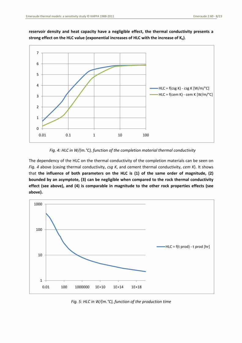
Emeraude thermal models: a sensitivity study © KAPPA 1988‐2011 Emeraude 2.60 ‐ 8/23
reservoir density and heat capacity have a negligible effect, the thermal conductivity presents a strong effect on the HLC value (exponential increases of HLC with the increase of Ke).
0
1
2
3
4
5
6
7
0.01 0.1 1 10 100
HLC = f(csg K) ‐ csg K [W/m/°C]HLC = f(cem K) ‐ cem K [W/m/°C]
Fig. 4: HLC in W/(m.°C), function of the completion material thermal conductivity
The dependency of the HLC on the thermal conductivity of the completion materials can be seen on Fig. 4 above (casing thermal conductivity, csg K, and cement thermal conductivity, cem K). It shows that the influence of both parameters on the HLC is (1) of the same order of magnitude, (2) bounded by an asymptote, (3) can be negligible when compared to the rock thermal conductivity effect (see above), and (4) is comparable in magnitude to the other rock properties effects (see above).
1
10
100
1000
0.01 100 1000000 1E+10 1E+14 1E+18
HLC = f(t prod) ‐ t prod [hr]
Fig. 5: HLC in W/(m.°C), function of the production time

Emeraude thermal models: a sensitivity study © KAPPA 1988‐2011 Emeraude 2.60 ‐ 9/23
The dependency of the HLC on the production time can be seen on Fig. 5 above. It shows that the longer the production time, the lower the HLC, i.e. the smaller the thermal conduction effect. Further remarks on the time dependency of the Segmented Model is given in a later section, when comparing both the Segmented Model and the Energy Model.
II.b.4 Fluid heat capacity Fig. 6 below shows the thermal profiles predicted by the Segmented Model when the produced fluid specific heat capacity (Cpg) increases from 0.043 Btu/(lbm.°F) ( ) to 9.9 Btu/(lbm.°F) ( ), the zone contributions being unchanged and identical on each zone (initial solution of the global improve). The calculated temperature profiles range from 163.7°F to 166.6°F.
Fig. 6: Temperature profiles for different Cpg Fig. 7: Temperature profiles for different Kg
Starting from the geothermal ( ) below the lower inflow, the dPJT value induces an important cooling over this inflow. It can be seen that the higher the fluid heat capacity, the lower the cooling effect on the inflow zones (the same can be seen on each inflow): the fluid heat capacity effect

Emeraude thermal models: a sensitivity study © KAPPA 1988‐2011 Emeraude 2.60 ‐ 10/23
counter balances the pressure drop effect on inflow zones, by facilitating convective heat transport by the fluid coming from below. Between the inflows, the temperature profile has a tendency to stay close to the temperature at the top of the inflow below when the fluid heat capacity is increasing: between the inflows, the fluid heat capacity tends to counter balance the thermal conduction , again by facilitating convective heat transport by the fluid coming from below.
II.b.5 Fluid thermal conductivity Fig. 7 above shows the temperature profiles predicted by the Segmented Model when the produced fluid thermal conductivity (Kg) increases from 0.01 W/(m.°C) ( ) to 40 W/(m.°C) ( ), the zone contributions being kept unchanged and identical on each zone. The calculated temperature profiles range from 164.2°F to 166.6°F.
It can be seen that increasing the fluid thermal conductivity has no influence on the thermal response given by the model.
II.b.6 Sensitivity summary The following table summarizes the effects identified when increasing the value of the different parameters considered in this sensitivity study.
Parameter Effect
dPJT Inflow zones: Cooling
HLC Between inflow: T. homogenizes and tends to geothermal
Fluid Cp Inflow zones: Between inflow:
T. homogenizes and tends to geothermal T. tends to the T. above or below (flow direction)
Fluid K No effect
Res. thermal cond. Between inflow: On HLC only – Large T. homogenizes and tends to geothermal
Production time Between inflow: On HLC only – Large T. tends to the T. above or below (flow direction)
Res. Cp and ρ Between inflow: On HLC only – Small
Casing thermal cond. Between inflow: On HLC only – Small
Cement thermal cond. Between inflow: On HLC only – Small
Tab.2: Segmented Model sensitivity to various parameters

Emeraude thermal models: a sensitivity study © KAPPA 1988‐2011 Emeraude 2.60 ‐ 11/23
III. Energy model
III.a. Theory In this model the wellbore is discretized into small well segments. Each segment is defined by its bottom pressure ( ) and temperature
( ), its bottom mass flow rate ( ) and its
mass contribution from the reservoir ( ).
Note that we refer hereafter to mass rates by and to volumetric rates by . The
wellbore/reservoir interface is defined by its pressure ( ) and temperature ( ), while
the reservoir is characterized, far from the well, by its geothermal temperature ( )
and by its average pressure ( ).
−sP
−sT
q
−sq
Q
sfT
isq
geoT
sfP
eP
Fig. 8: well discretization
III.a.1 Mass balance The mass balance equation applied to each segment gives:
Where )2
,2
(~ −− ++= ssss TTPPρρ denotes the average segment density.
III.a.2 Energy balance Energy conservation equations can be written for the individual well segments on the one hand, and for the reservoir part on the other hand. We will refer to these equations as E1 and E2 respectively, and expressions are given below for different flow directions. The resulting set of equations needs to be solved simultaneously for the couple of unknown ( ), which is performed by an iterative
method until convergence is achieved. sfs TT ,
For a producer, the temperature is updated starting from the lowest producing segment and going up the well to the top reservoir. For an injector, it is updated from the injection point going down the well.
The schematics below are respectively showing three different configurations: a producer (Fig. 9a), a producer with thief(s) inflow zones (Fig. 9b), and an injector (Fig. 9c). The corresponding equations
are given next, where tildes denote averaged segment quantities and , . 2wrA ⋅= π dLrA wsf ⋅= π2
−−− ⋅+⋅=+= ssississ QQqqq ρρ~

Emeraude thermal models: a sensitivity study © KAPPA 1988‐2011 Emeraude 2.60 ‐ 12/23
(Fig. 9a)
(Fig. 9b)
(Fig. 9c)
( ) 0~22
12
12
12
2
22
2
22
2
2 =−⋅+⎟⎟⎠
⎞⎜⎜⎝
⎛⋅−⋅+⋅+⎟
⎟⎠
⎞⎜⎜⎝
⎛⋅+⋅−⎟
⎟⎠
⎞⎜⎜⎝
⎛⋅−⋅+⋅
−
−−−− ssfwb
sf
is
sfsfis
s
sss
s
ssss TTDdlgq
Ahqq
Ahqdlgq
AhQ
ρρρρ1 =E
a) Energy equations for a producer (Fig. 9a):
b) Energy equations for a producer with a thief zone (Fig. 9b):
c) Energy equations for a injector (Fig. 9c):
The energy balance in each well element (E1) includes convective heat fluxes (the internal, kinetic and potential energy being transported by fluid movement from / to the segment below, above and the reservoir), as well as conductive heat flux between the wellbore sand face and the segment itself. The reservoir energy balance (E2) considers convective heat fluxes (the internal, kinetic and potential energy being transported by fluid movement from / to the well segment), as well as
( ) ( ) 0~2
12 2
2
2 =−⋅+−⋅+⎟⎟⎠
⎞⎜⎜⎝
⎛−⋅+⋅= geosfresssfwbres
sf
is
sfsfis TTDTTDhq
AhqE
ρ
( ) 0~2~2
1~2
12
12
2
22
2
22
2
2 =−⋅+⎟⎟⎠
⎞⎜⎜⎝
⎛⋅+⋅+⋅−⎟
⎟⎠
⎞⎜⎜⎝
⎛⋅+⋅−⎟
⎟⎠
⎞⎜⎜⎝
⎛⋅−⋅+⋅
−
−−−− ssfwb
is
sfis
s
sss
s
ssss TTDdlgq
Ahqq
Ahqdlgq
AhQ
ρρρρ1=E
( ) ( ) 0~~2
1~2 2
2
2 =−⋅+−⋅+⎟⎟⎠
⎞⎜⎜⎝
⎛−⋅+⋅−= geosfresssfwbres
is
sfis TTDTTDhq
AhqE
ρ
( ) 0~2~2
1~2
12
11 2
2
22
2
22
2
2 =−⋅+⎟⎟⎠
⎞⎜⎜⎝
⎛⋅−⋅+⋅−⎟
⎟⎠
⎞⎜⎜⎝
⎛⋅+⋅+⋅+⎟
⎟⎠
⎞⎜⎜⎝
⎛⋅+⋅−= ++
−
−−− ssfwb
is
sfis
s
ssss
s
sss TTDdlgq
Ahqdlgq
AhQq
AhqE
ρρρ
ρ
( ) ( ) 0~~2
1~2 2
2
2 =−⋅+−⋅+⎟⎟⎠
⎞⎜⎜⎝
⎛−⋅+⋅−= geosfresssfwbgeo
is
sfis TTDTTDhq
AhqE
ρ

Emeraude thermal models: a sensitivity study © KAPPA 1988‐2011 Emeraude 2.60 ‐ 13/23
conductive heat flux between the wellbore sand face and the segment itself, and between the wellbore sand face and the reservoir. The conductance terms, D’s, are computed based on the well completion and reservoir parameters information (see HLC calculation below). In these equations, the enthalpies (h), densities (ρ) and flow rates (q, Q) are those of the fluid mixture.
Finally, to close the system, the external sand face, , and the reservoir pressure, , must be
known: these can either be user inputs or calculated by Emeraude on the basis of the well and the reservoir description (see Pressure drop calculation below).
sfP eP
III.a.3 Heat loss coefficient calculation The thermal conductance terms are defined as:
)/ln(/2*weresres rrdLD ⋅⋅= πλ
wwb rdLUD ⋅⋅⋅= π2
The Heat Loss coefficient (HLC) is defined as wrUHLC ⋅⋅= π2 where the Heat Transfer Coefficient,
U, is evaluated from the general formulae:
)(
lnlnlnln1
rcci
to
cem
co
wto
c
ci
coto
ann
to
cito
t
ti
toto
hhrr
kr
rr
kr
rr
kr
rr
kr
rr
U ++
⎟⎠⎞⎜
⎝⎛
+⎟⎠⎞⎜
⎝⎛
+⎟⎠⎞⎜
⎝⎛
+⎟⎠⎞⎜
⎝⎛
=
Where denote thermal conductivities and terms and are corrective terms accounting for
the annulus free convection and the annulus radiation respectively (Hassan and Kabir, 2002). Note that the presence of these corrective terms for the annulus introduces a dependence of U on the temperature, increasing the nonlinearity of the system, which may lead to a large increase in computational time. It is hence recommended NOT to use these corrections unless for very specific problems such as when the annulus is filled with gas.
k ch rh
Neglecting the free convection and radiation in the annulus, we can rewrite
)2()1(
)2()1(
1
2
ln
2
ln
2
ln
2
ln
wbwb
wbwb
cem
co
w
c
ci
co
ann
to
ci
t
ti
to
wb DDDD
kr
r
kr
r
kr
r
kr
r
dLD+⋅
=
⎥⎥⎥⎥
⎦
⎤
⎢⎢⎢⎢
⎣
⎡
⋅
⎟⎠⎞⎜
⎝⎛
+⋅
⎟⎠⎞⎜
⎝⎛
+⋅
⎟⎠⎞⎜
⎝⎛
+⋅
⎟⎠⎞⎜
⎝⎛
⋅=
−
ππππ
1
)1(
2
ln
2
ln−
⎥⎥⎥⎥
⎦
⎤
⎢⎢⎢⎢
⎣
⎡
⋅
⎟⎠⎞⎜
⎝⎛
+⋅
⎟⎠⎞⎜
⎝⎛
⋅=ann
to
ci
t
ti
to
wb kr
r
kr
r
dLDππ
1
)2(
2
ln
2
ln−
⎥⎥⎥⎥
⎦
⎤
⎢⎢⎢⎢
⎣
⎡
⋅
⎟⎠⎞⎜
⎝⎛
+⋅
⎟⎠⎞⎜
⎝⎛
⋅=cem
co
w
c
ci
co
wb kr
r
kr
r
dLDππ

Emeraude thermal models: a sensitivity study © KAPPA 1988‐2011 Emeraude 2.60 ‐ 14/23
Where accounts for tubing and annular, and accounts for casing and cement. Note that
the first term needs a thermal conductivity for the annular and should be taken into account only when the static annular fluid is known (typically only above the production packer).
)1(wbD )2(
wbD
If the annular/tubing term is not to be taken into account (infinite conductivity): . )2(wbwb D=D
In the special case of a tubing leak into the annulus, the thermal conductivity of the annulus is taken as equal to that of the flowing fluid mixture in the annulus.
III.a.4 Pressure drop calculation In the absence of prescribed external pressure needed to compute the enthalpy (see equation E2 above), one can try to back‐calculate this pressure based on the well skin (S), the geometry of the perforations and the reservoir characteristics.
These pressure drops are computed iteratively at the average pressure point and at flowing wellbore temperature, in order to fulfill:
The viscosity is the mixture viscosity at the average pressure. The external pressure is then computed iteratively:
Positive skin
Negative skin
])ln([2
)(G
T
THsese S
rwreS
Lwh
hkQPPP ++⋅⋅
⋅⋅⋅
=−=Δπ
μ
])[ln(2
)(
][2
)(
};{|
};{|
GTH
TPsfe
T
TH
TPssf
Srwre
hkQ
PP
SLwh
hkQ
PP
sR
sW
+⋅⋅⋅
⋅+=
⋅⋅⋅⋅
⋅+=
πμ
π
μ
])[ln(2
)( };{| SLwhS
rwre
hkQ
PP
PP
TG
TH
TPsfe
ssf
sR ⋅++⋅⋅⋅
⋅+=
=
πμ

Emeraude thermal models: a sensitivity study © KAPPA 1988‐2011 Emeraude 2.60 ‐ 15/23
The Pseudo‐skin, SG, depends on the slant, the anisotropy, the geometry of the perforations and the formation. It is evaluated from Chen et al. (1995), with an anisotropic correction from Pucknell & Clifford (1991).
III.b. Sensitivity analysis As described above, several parameters are governing the Energy Model predictions: ‐ Reservoir geophysical properties: on the inflows. Govern the heat transport by the moving
fluids from or to the reservoir. This includes the Joule‐Thomson effect. ‐ Heat loss coefficient (HLC): over the entire well. Governs the thermal conduction across the
completion. ‐ Reservoir thermal properties: over the entire well. Govern the thermal conduction across the
reservoir.
The following presents the influence of these parameters on the Energy Model predictions, as well as the influence of other parameters on the HLC. As for the Segmented Model, this has been obtained by running several cases on a single phase gas producer (methane), with three contributing zones corresponding to Emeraude Guided Session B10.
III.b.1 Reservoir thermal conductivity Fig. 10 below shows the temperature profiles predicted by the Energy Model when the reservoir thermal conductivity (Ke) increases from 0.1 W/(m.°C) ( ) to 1000 W/(m.°C) ( ), the zone contributions being unchanged. The calculated temperature profiles range from 163.9°F to 166.6°F.
Starting from the geothermal ( ) below the lower inflow, a cooling can be seen over this inflow: it corresponds to an important pressure drop across the reservoir. One can notice that the higher the reservoir thermal conductivity, the lower the cooling. Then, between the bottom inflow and the middle one, the temperature predicted by the Energy Model tends to the geothermal value, and this tendency increases with Ke.
As the reservoir thermal conductivity increases, the temperature in the well homogenizes faster and tends towards the geothermal value. This effect can become predominant.
III.b.2 Reservoir radius Fig. 11 below shows the temperature profiles predicted by the Energy Model when the reservoir radius (re) increases from 0.03 ft ( ) to 1e5 ft ( ), the zone contributions being unchanged. The calculated temperature profile ranges from 163.9°F to 166.6°F.
In essence, this would mean that the geothermal profile is reached further away from the wellbore with an increase in the reservoir radius: for a given set of parameters, the bigger the reservoir radius, the lower the temperature homogenization due to conduction. This effect is expected to be opposite to that of the production time, because the larger the production time, the closer the geothermal to the wellbore.

Emeraude thermal models: a sensitivity study © KAPPA 1988‐2011 Emeraude 2.60 ‐ 16/23
Fig. 10: Temperature profiles for different Ke
Fig. 11: Temperature profiles for different re
III.b.3 Fluid heat capacity Fig. 12 below shows the temperature profiles predicted by the Energy Model when the produced fluid heat capacity (Cpg) increases from 0.043 Btu/(lbm.°F) ( ) to 9.9 Btu/(lbm.°F) ( ), the zone contributions being unchanged and identical on each zone. The calculated temperature profiles range from 164.2°F to 166.6°F.
It can be seen that at each depth, the temperature below propagates in an easier way: increasing the fluid heat capacity strongly reduces the Joule Thomson cooling effect. This facilitates the heat transport by convection along the wellbore.
III.b.4 Heat loss coefficient Fig. 13 below shows the temperature profiles predicted by the Energy Model when the HLC increases from 0.06 W/(m.°C) ( ) to 630 W/(m.°C) ( ), the zone contributions being unchanged. The calculated temperature profiles range from 164.1°F to 166.6°F.

Emeraude thermal models: a sensitivity study © KAPPA 1988‐2011 Emeraude 2.60 ‐ 17/23
Starting from the geothermal ( ) below the lower inflow, a cooling can be seen over this inflow: it corresponds to an important pressure drop across the reservoir, independent of the value of the HLC. Then, between the bottom inflow and the middle one, the temperature predicted by the Energy Model tends to the formation temperature close o the wellbore with increasing HLC values.
As the HLC increases, the temperature homogenizes faster and tends towards the sandface temperature, this effect strongly limited by small reservoir thermal conductivity (Ke) which tends to limit the temperature difference between the sandface and the flowing fluid in the wellbore. The HLC effect would be more pronounced for larger Ke or smaller values of production time, for which the sandface temperature profile would be closer to the geothermal one.
Fig. 12: Temperature profiles for different Cpg
Fig. 13: Temperature profiles for different HLC

Emeraude thermal models: a sensitivity study © KAPPA 1988‐2011 Emeraude 2.60 ‐ 18/23
III.b.5 Parameters acting on the HLC Different parameters act on the HLC value, such as the thermal conductivity of the completion materials, and the completion geometry.
The dependency of the HLC on the thermal conductivity of the different completion materials can be seen on the Fig. 14 (casing thermal conductivity, csg K, and cement thermal conductivity, cem K). The plot shows that influence of both parameters on the HLC presents the same behavior, and is limited by an asymptote. For common materials, the influence of the casing (or tubing) is usually predominant (the inverse would correspond to unrealistic cement conductivities).
Fig. 14: HLC in W/(m.°C), function of the completion material thermal conductivity
The dependency of the HLC on the completion geometry can be seen on Fig. 15 (ratios of internal diameter, ID, to outer diameter, OD). This plot shows that influence of the casing thickness, tubing (by extension) and cement is of the same order of magnitude, and that the HLC highly increases with a decreasing annulus space between the casing and the cement.
0
500
1000
1500
2000
2500
3000
3500
4000
4500
0.01 0.1 1 10 100 1000 10000 100000
HLC = f(csg K) ‐ csg K [W/m/°C]
HLC = f(cem K) ‐ cem K [W/m/°C]

Emeraude thermal models: a sensitivity study © KAPPA 1988‐2011 Emeraude 2.60 ‐ 19/23
Fig. 15: HLC in W/(m.°C), function of the completion geometry
III.b.6 Parameters acting on heat transport from/to the reservoir Heat transport due to the fluid moving from the inflow zones to the well (or reverse), strongly depends on the pressure drop across the considered reservoir zones. In addition, the Joule‐Thomson effect can also play a role.
As explained earlier, Emeraude allows the user proceeding with one of the following choices:
0
500
1000
1500
2000
2500
3000
3500
4000
0 0.2 0.4 0.6 0.8 1
HLC = f(Csg ID / Csg OD)
HLC = f(Csg OD / Cem OD)
HLC = f(Csg ID / Cem OD)
1‐ Directly enter a pressure drop value for each inflow 2‐ Give the geophysical properties for each inflow together with the well skin, and let Emeraude
calculates the corresponding pressure drop
With unchanged zone contributions, each temperature track on Fig. 16 shows, from left to right, the temperature profiles when increasing the following parameters over the top inflow:
• The pressure drop: from 1 psi to 150 psi, • The permeability: from 0.1 mD to 1000 mD, • The vertical to radial permeability ratio: from 0.0001 to 1, • The porosity: from 0.001 to 1, • The skin: from ‐20 to 20.

Emeraude thermal models: a sensitivity study © KAPPA 1988‐2011 Emeraude 2.60 ‐ 20/23
Fig. 16: Temperature profiles for varying geophysical parameters
The white arrows show the temperature profile evolution for an increase of the above parameters. They point to the left for an increase in the observed temperature cooling, and to the right for a decrease in the observed temperature cooling. The temperature varies between 157°F and 166.6°F.
It can be seen on the first temperature track that, as expected, the larger the pressure drop, the larger the cooling.
The second temperature track shows that an increase in the reservoir permeability reduces the cooling: this is because the pressure drop required to achieve the zone contribution is reduced when the permeability increases. Hence, the larger the permeability, the lower the cooling.
The third temperature track shows that, for a partially perforated interval, an increase in the vertical to radial permeability ratio reduces the cooling; the amplitude of the reduction being bounded. Again, this is because the pressure drop required to reach the zone contribution is reduced when the vertical permeability increases. Hence, for a partially perforated interval, the bigger the vertical to radial permeability ratio, the lower the cooling (although bounded). Note that, because the flow is only radial to the well when considering a fully perforated interval, there will be no impact of the permeability ratio on the amplitude of the temperature cooling.
The fourth temperature track shows that a porosity change has no significant effect on the temperature cooling.
The fifth temperature track shows that an increase of the skin value increases the temperature cooling. This is because the pressure drop required to reach the zone contribution is increased when

Emeraude thermal models: a sensitivity study © KAPPA 1988‐2011 Emeraude 2.60 ‐ 21/23
the skin increases. Hence, the bigger the skin, the bigger the temperature cooling. On the contrary, highly negative skin values induce a small temperature cooling and at a given depth, the temperature is strongly influenced by the temperature of the preceding point in the direction of the flow: for high negative skins, the heat transport by convection along the well dominates.
III.b.7 Sensitivity summary The following table summarizes the effects identified when increasing the value of the different parameters considered in this sensitivity study.
Parameter Effect
Ke Can be large T. homogenizes and tends to geothermal
Res. radius Limits conduction Limits T. tendency to geothermal
Fluid Cp Facilitates convection along the well
T. tends to T. above or below (dep. flow dir.)
HLC Bounded effect T. homogenizes and tends to geothermal
Kcsg, Ktbg, Kcem Through the HLC The cement effect is the least
Material thickness Through the HLC Slightly increasing when annulus space decreases
dP Inflow zones: Increases the cooling
Permeability Inflow zones: Reduces the cooling
Permeability ratio Inflow zones: Partially perforated intervals: reduces the cooling Fully perforated intervals: no effect
Skin Inflow zones: Increases cooling High negative skin facilitates convection along the well
Porosity Inflow zones: No effect
Tab.3: Energy Model sensitivity to various parameters

Emeraude thermal models: a sensitivity study © KAPPA 1988‐2011 Emeraude 2.60 ‐ 22/23
IV. Influence of other parameters
IV.a. Time dependency Time dependence of the models is taken into account only when considering the heat transport by conduction: it appears in the expression of the HLC. The following tracks show the evolution of the temperature profile at different production times in a single phase case, with one producing interval at the very bottom: the geothermal profile is in red, the Energy Model prediction in blue and the Segmented Model prediction in green.
Temperature profiles at different production times predicted by both models
The Energy model solution appears to be more physically acceptable, as it is bounded, whereas the Segmented Model predicts a continuous increase of the temperature over the depth interval, due to the unlimited conduction effect carried over by the HLC.
IV.b. Annular free convection The Energy Model allows considering annular free convection when evaluating the heat transfer. This is often negligible, but it may have a significant impact on the solution when the annular fluid is particularly sensitive to the thermal gradient existing across and along the well (typically, when invaded with gas).
The following plot shows the multiphase field case described by Hassan & Kabir in SPE 22948. The red dots correspond to the measurements, the blue curve to the Energy Model without considering the annular free convection, and the green curve considering annular free convection.

Emeraude thermal models: a sensitivity study © KAPPA 1988‐2011 Emeraude 2.60 ‐ 23/23
Geothermal ( ) and temperature profiles with ( ) and without ( ) free convection compared
to measurements ( )
This shows the importance of the annular free convection and it also provides a good assessment of the Energy Model in multiphase flow (the single phase case has been checked versus a Rubis simulation, see Emeraude guided session B10).