thermo-viscous effects on finite amplitude sound...

Thermo-viscous effects on finite amplitude sound propagation in a rectangular waveguide

M.J. Anderson

Department of Mechanical Engineering, Universityof Idaho, Moscow, Idaho 83843

P.G. Vaidya Department of Mechanical and Materials Engineering, Washington State University, Pullman, Washington 99164-2920

(Received 23 August 1990; accepted for publication 4 April 1991 )

The role that thermo-viscous effects play in the propagation of finite level sound in a waveguide has been reexamined from a fundamental perspective. In the past, nonlinear acoustic interactions have been described by energy conserving modulation of spectral amplitudes as wave packets travel axially down the waveguide. To account for thermo-viscous effects in this modulation, investigators have included without formal justification into the modulation equations dissipative terms with a magnitude corresponding to the Kirchhoff rate of attenuation encountered in linear theory. In this investigation, the problem of the propagation of finite magnitude p, lane waves is analyzed in a different manner. As opposed to previous investigations, all three modes (acoustic, vorticity, and entropy) are considered from the outset. The boundary conditions are extended to 'include vanishing normal and tangential fluid velocity, as well as vanishing fluid temperature perturbations. A new solution at second order is presented (second order being the first correction due to nonlinearity), which is uniform in the spatial variables. As a consequence, it is shown that the thermo-viscous effects are incorporated into the spectral amplitude modulation equations through one of the boundary conditions. These modulation equations apply to both plane and higher-order modes, including the region arbitrarily near the cutoff frequency for the higher-order modes. It is shown that the small parameter 1/x/•, where N = poDc/p (the acoustic Reynolds number), is a special scale for analysis of nonlinear interactions in a waveguide. In particular, the relative magnitude of the sound source and l/f•- is a determining factor that predicts whether nonlinear interactions will be significant.

PACS numbers: 43.25.Jh, 43.20. Mv

INTRODUCTION

The behavior of finite level sound propagating in a waveguide has been the object of several investigations. These investigations have shown that when sound levels become finite (say greater than 125 dB re: 20pPa in air at 200 Hz), the effects of nonlinearity under quite general circumstances become measurably significant. Because of this fact, the prediction of the qualities of the nonlinear effects are of practical engineering importance.

It has been known for some time that finite level plane waves at all frequencies will mutually interact in a rectangular waveguide, generating sum and difference harmonics as a result of their interaction. •'• Using various techniques, it was shown that the interactions are described by an infinite set of bilinear first-order differential equations governing the amplitude of each plane wave, • or a similar nonlinear coordinate transformation, 2 each dependent upon the axial distance traveled by the waves. In this theory, the interaction of plane waves is energy conserving, and therefore identical with the behavior associated with the Earnshaw solution)

Furthermore, the behavior of finite level higher-order modes has also been investigated using the same methodologies as for the plane modes. Vaidya and Wang 4 and Gins-

berg 2 have shown that a particular subset of higher-order modes will interact, this subset being those higher-order modes having equal phase velocity. The amplitudes of these modes were also observed to modulate as the waves travel

axially down the waveguide, the modulation being determined by bilinear first-order differential equations or equiv- alent nonlinear coordinate transformations. Again, this theory predicted energy conservant nonlinear interactions.

In all of the preceding investigations, the fluctuations occurring in the waveguide were presumed to be governed by a nonlinear wave equation that includes the effect of quadratic nonlinearity originating from the continuum equations but ignores dissipation and requires that the velocity fluctuations be isentropic and irrotational. In effect, these methodologies neglected the presence of the vorticity and entropy modes. As a consequence, the boundary condition applied at the waveguide walls is vanishing normal velocity. This means that the viscous and thermal boundary layer processes are not included in the problem solving philosophy from the beginning. To achieve practical results, however, Vaidya and Wang 4 and Hamilton and TenCate 5 have ac- counted for the boundary layer processes by incorporating dissipative terms in the first-order differential equations that

1056 J. Acoust. Soc. Am. 90 (2), Pt. 1, August 1991 0001-4966/91/081056-12500.80 @ 1991 Acoustical Society of America 1056

model the attenuation presumed to effect the nonlinear mod- u!ation of the interacting higher-order modes.

An exception to the methodologies adopted in the previously described work is the investigation undertaken by Burns 6 in the 1960s. Burns calculated the sound field that

would occur in a cylindrical tube with a source generating fluctuations that are finite in magnitude. In his investigation, Burns required the normal and tangential velocity fluctuations to vanish at the boundaries, as well as the fluid temperature perturbations. The method applied by Burns to this problem was straight perturbation expansion, and as a consequence his solution c(•ntained secular terms. Due to the complexity of the procedure, only results for plane modes were presented, although in principle the procedure could be applied to determine the nonlinear interaction of higher-order modes as well. It was found that acoustic boundary layer processes did alter the nonlinear modulation of the plane waves that were considered.

In the present investigation, we will reexamine the problem of finite level sound propagation in a waveguide from a fundamental perspective. This perspective will incorporate the viscous and thermal boundary layer processes directly into the development of the equations that describe the nonlinear interaction of plane waves by including the vorticity and entropy modes in the analysis. Inclusion of the entropy and vorticity modes will require that the boundary conditions at the waveguide wall are vanishing normal and tangential velocity, and continuity of temperature (in this case, we will consider the waveguide wall material to be a much better conductor of heat than the medium inside the wave-

guide). The new perspective is made possible by a discovery ? in the application of the method of multiple scales to the corresponding problem of the propagation of linear sound in the same waveguide. The main results of the subsequently described work have been presented in a separate docu- ment. s

I. PROBLEM DEFINITION AND GOVERNING EQUATIONS

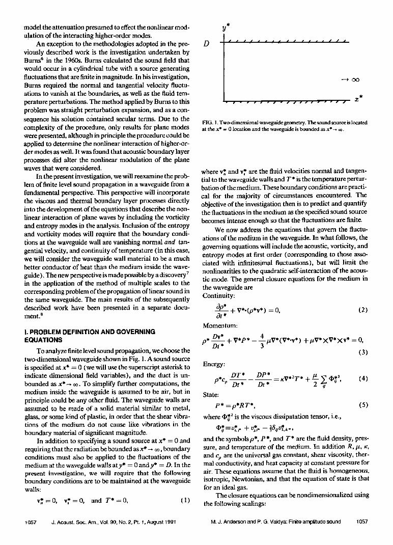
To analyze finite level sound propagation, we choose the two-dimensional waveguide shown in Fig. 1. A sound source is specified at x* = 0 (we will use the superscript asterisk to indicate dimensional field variables), and the duct is unbounded as x*--, oo. To simplify further computations, the medium inside the waveguide is assumed to be air, but in principle could be any other fluid. The waveguide walls are assumed to be made of a solid material similar to metal,

glass, or some kind of plastic, in order that the shear vibrations of the medium do not cause like vibrations in the

boundary material of significant magnitude. In addition to specifying a sound source at x* = 0 and

requiring that the radiation be bounded as x*-• 0o, boundary conditions must also be applied to the fluctuations of the medium at the waveguide walls aty* = 0 andy* = D. In the present investigation, we will require that the following boundary conditions are to be maintained at the waveguide walls:

v,=0, v,*=0, and T*=0, (1)

D

FIG. 1. Two-dimensional waveguide geometry. The sound source is located at the x* = 0 location and the waveguide is bounded as x*

where %* and v,* are the fluid velocities normal and tangential to the waveguide walls and T* is the temperature perturbation of the medium. These boundary conditions are practical for the majority of circumstances encountered. The objective of the investigation then is to predict and quantify the fluctuations in the medium as the specified sound source becomes intense enough so that the fluctuations are finite.

We now address the equations that govern the fluctuations of the medium in the waveguide. In what follows, the governing equations will include the acoustic, vorticity, and entropy modes at first order (corresponding to those associated with infinitesimal fluctuations), but will limit the nonlinearities to the quadratic self-interaction of the acoustic mode. The general closure equations for the medium in the waveguide are Continuity:

Op_•_* + V*-(p*v*) = O, (2) Ot*

Momentum:

p, Dr* • --+ V'P*-- pV*(V*.v*) +/t?*X?*Xv* = O, Dt *

(3)

Energy:

DT* DP* -- •cV*"T* +•- • •, (4) ,o*% Dt * Dt * .. State:

P* =p*RT*, (5)

where (I)•. 2 is the viscous dissipatation tensor, i.e., *• * 2 • •i• -vi.r + v•.,, - •SijVk.k*,

and the symbols p*, P*, and T* are the fluid density, pressure, and temperature of the medium. In addition R, p, •, and c•, are the universal gas constant, shear viscosity, thermal conductivity, and heat capacity at constant pressure for air. These equations assume that the fluid is homogeneous, isotropic, Newtonian, and that the equation of state is that for an ideal gas.

The closure equations can be nondimensionalized using the following scalings:

1057 J. Acoust. Sec. Am., Vol. go, No. 2, Pt. 1, August 1991 M.J. Anderson and P. G. Vaidya: Finite amplitude sound 1057

P* -P• p* - po* v* P-- , p----, v=--,

PO* po* c

T* -- TO* T-- ,

To*

t- , (x,y,z) = - , , , D D

where the "0" subscript denotes the ambient value of a field variable. In the above scalings, c is the isentropic speed of sound and D is a length scale that corresponds to the width of the waveguide under consideration. Implementation of the above scalings into the closure set [ (2)-(5)] results in the oa following nondimensional equations that govern the fluctuations in the waveguide: oat Continuity:

OaP + V.v + V-(pv) = 0, (6) Momentum:

Dv 1

(p + 1) -•- +--¾P------

Energy:

4 1

3N V(V.v) + •VXVXv = 0, (7)

DT y-- 1 DP (p+ 1)

Dt 7/ Dt

_ I V2T_ • 1 c 2 • NPr N cpTo •'•' (8) State:

p= (P+ 1)/(T+ 1) - 1, (9)

where 7/is the ratio of specific heats, Pr is the Prandtl number, and N = po*Dc/g is the acoustic Reynolds number of the fluid, in this case air. The nondimensional set (6-9) retains all information associated with fluid motions.

In the subsequent analysis, the set [(6)-(9)] will be analyzed using the perturbation method of multiple scales. In this context, nonlinear terms will be retained only through quadratic order. In general, the dependent variables will be expanded in a sequence similar to

Or= al + -- a2 + --

1

where a is a field variable and the quantity 1/x•- is the scale used in the expansion. Furthermore, similar expansions with the same scale will be applied to chosen independent variables when necessary. As a consequence, if interest is re- stricted to the first correction due to nonlinearity, all activity of magnitude less than O(l/N) can be neglected.

In the Appendix, it is shown that if the two-dimensional fluid velocity and temperature fluctuations are decomposed according to

v=V• +Vde+ Vx(;ez), (10)

T = - (7/- 1) + •VP oat 2

+ NPr• + (3Pr-1) oa&• oa----•-, (11) then the closure equations can under certain assumptions be reduced to

Vorticity:

oat 1_ V=; = 0, (12) 8t N

Acoustic:

+ I 7/-- I ,

= oaT \ at / + Vq•a.Vq•a , (13) Entropy:

8• 1 V2•e = 0. (14) Ot N Pr

The decomposition (10) splits the velocity field into its compressible and incompressible pa•itions, with the compressible partition further subdivided into those which pre- dominantly generate entropy, and those that do not. As such, 4, corresponds to the acoustic mode, 4• corresponds to the entropy mode, and • corresponds to the yogicity mode. In the set [ ( 12)-(14) ], only the nonlinear self-interaction of the acoustic mode has been retained. Quadratic products containing 4• and • have been ignored. The precise terns that have been eliminated are stated in the Appendix.

The fluid velocity and temperature decompositions [ ( 10),( 11 ) ] then allow the boundary conditions ( 1 ) for a two-dimensional waveguide to be written in terms of the field variables •, 4e, and • as

--+• •-o, (•) & & Ox

NPr• -- (Z-- 1) •" =0. (17) Ot

In the temperature boundary condition (17), only the leading-order terms in the decomposition (11) have been retained. The higher-order terms do not contribute to the problem solution because of the nature of the perturbation expansion to be described in the subsequent section.

II. PERTURBATION ANALYSIS OF THE FINITE LEVEL FLUCTUATIONS

The boundary value problem will be solved first for plane-wave sources with the perturbation method of multiple scales. ø Solutions for higher-order modes will then be stated. For the higher-order modes, it will be seen that the results will apply even in the case that the frequency is arbitrarily near the cutoff frequency. In both cases, a special expansion of the independent and dependent variables using

1058 J. Acoust. Soc. Am., Vol. 90, No. 2, Pt. 1, August 1991 M.J. Anderson and P. G. Vaidya: Finite amplitude sound 1058

the acoustic Reynolds number Nasa scale will be used. This expansion was applied successfully to the associated linear problem. ? The expansion used for the perturbation analysis is

qSa = 1 qS•, (x,g,y,t) + ½•2 (x,g,y,t)

+ "' + qL• (x,•,y,t), (18)

I • 1

+ '" + ½,, (x,•,rl,y,t), (19)

1 2 1

= (•-)•2(x,•,rl,y,t) • (•)•,(x,•',rl,y,t)+ +'" + ½n (X,½,'t,y,t), (20)

where the new axial and tranverse coordinates ½ and r/are

• = --, (21a)

•/= .V•5•. (2lb) Note that the entropy and vorticity modes begin at smaller orders in magnitude as would be calculated in the case of infinitesimal fluctuations. The above expansions [( 18)- (20)] will effectively sort out the effects of singularity (in the entropy and vorticity modal equations) and nonlinearity (in the acoustic mode equation).

After substitution of the above expansions [ (18)-(20) ] into the modal equations [ ( 12)-(14) ] and boundary conditions [(15)-(17)] and upon subsequently equating the coeftiecients of ( 1/x/-ff) • we obtain the following sequential system of problems:

02½o• 02½• O•a• •-I- -- ax • • Ot •

BCs:

Pr• -- (•- 1) 0• =0, Ot

-- 0•

=-2 •+(y-1)•• Ot a9t •

(23a)

(23b)

(23c)

(25)

=0, (26a)

a.,,: =ø' and following at higher orders in the coefficient 1/x/-•,

(26b)

(26c)

(27)

--= o, (28)

--=0. (29)

The above sequential (BCs) set [ (22)-(29) ] of equations and boundary conditions is the same that results from application of the just described perturbation analysis to the linear problem, with the exception of the extra forcing terms due to nonlinear interactions for the acoustic mode (24). Note that due to the expansions [ (18)-(20) ] chosen for the velocity potentials, the nonlinear sources for the acoustic mode are O(l/N), well within the range of accuracy for the modal decomposition. The source terms for the acoustic mode have been identified as being resonant for plane waves, and eventually lead to manifestations of nonlinear behavior in

(22) The manner in which the boundary conditions [ (23),(26) ] appear in the problem gives special insight into the solution. At O(l/f•), the first-order acoustic mode is entirely determined by the boundary condition c•½o•/r•y = [(23b)]. The first-order quantities 4• and • are then uniquely determined by their governing equations [(25),(28)] and the remaining boundary conditions [ (23a),(23c) ]. At second order, we observe that the acoustic mode •2 is uniquely determined by its governing equation (24) and the associated boundary condition (26b), because thefirst-order quantities • and ½• are already known. This means that the first correction to the acoustic mode due to nonlinearity is determined by the quadratic sources present in the equation and the first-order vorticity and entropy modes.

Returning now to the solution of the problem for plane waves, we identify the solutions of the lowest-order set [ (22),(25),(28) ] subject to the boundary conditions (23). We choose a superposition of plane waves and calculate the

(24) associated vorticity and entropy mode components

1059 d. Acoust. $oc. Am., Vol. 90, NO. 2, Pt. 1, August 1991 M.d. Anderson and P. G. Vaidya: Finite amplitude sound 1059

q•,• = • A,(2)e i"'ø(" ') A- [c.c.], (30)

Xe i"'ø(x-'• + [c.c.], (31)

q• _ iw(y-- 1) • nAn(•)(•,o + •n•) Pr .= •

•e •-• + [v.c.], (32)

where [c.c.] denotes the complex conjugate and the voni- city and entropy transverse mode shapes are

•o = exp( -- [ ( 1 - i)•/•]

•.• = exp(-- [(1 -- i)•/•] (•-- V)),

= - [ -

- [(1 - - In the above fo•ulations, the frequency has been nondimensionalized according to w = w*D/c. The supe•osition of plane waves (30) contains an infinite set at hamonics n = 1 ..... •, where w represents the "lowest common denominator." The infinite set is necessary because nonlinear effects will generate sum and difference frequencies from the fundamental (the fundamental being the ha•onics present at the source, x • • = 0) ad infinitum. For example, if two harmonics of 1• and 110 Hz are present at the source, then the lowest common denominator frequency is 10 Hz, which corresponds to the difference frequency. Note that the coefficients A,0) must be chosen so that the coe•cients •nwA• (0)• are of such magnitude to ensure a convergent series for specification of fluid velocity at the source.

Now we proceed to solve the first correction system for the plane-mode source at the next higher order. Focusing first on the acoustic mode, we place the first-order solution 4• into (24) to obtain

8x • Oy • 8t •

•e •(•-" + [c.c.], (33)

where

n-- 1

• • • k(n - •)•_• k•l

• • kn(n-k)•_•A•, k=n+l

the overbar indicates the complex conjugate, and the prime indicates the derivative of a function with respect to its argument. The bilinear • term represents the nonlinear self- interaction of the acoustic mode.

It is immediately evident that the acoustic mode equation (33) is apparently resonant, which has been pointed out previously in the literature. The resonance manifests itself in a solution for • that goes as

• •xd •- '• • [c.c.], (•4)

which is unbounded as x • •. Hence, the prevailing opinion has been to interpret the forcing terms in (33) as secular, and use the removal of secularity as the condition to determine the functional dependence of the modal coefficients A, (2) on the slow coordinate 2. Removal of the secular forcing terms in (33) will then result in the ordinary differential equations

A•(2)=[o.•2(y+l)/2n]tb,, n=l ..... •o. (35)

These equations determine the modulation of the source spectra as it travels axially down the duct. It can be shown that they are energy conservant in nature, and in fact correspond to the Earnshaw solution for plane waves as pointed out by Ginsberg/ Consequently, they do not include the viscous and thermal boundary layer processes. These equations, however, have been in the past supplemented with dissipation terms that model viscous and thermal boundary layer processes as pointed out in the Introduction.

In a previous application of the method of multiple scales to the corresponding linear problem, 7 it was pointed out that the unbounded solution (34) at second order is not the only one available. In fact, it can be shown that

1 •2ointø(x -- t) X(y--•, • + [c.e.] (36)

is also a solution of the apparently resonant acoustic mode equation (33). The alternative solution (36) is bounded in magnitude throughout the domain of independent variables, so that the perturbation expansion (18) for • is globally uniform (at least through order l/N).

To complete the specification of •2 using the alternative form (36), we place •b•2 into the balance of normal velocities (26b), which results in the ordinary differential equations

A '. (2) --

+w•(Y+l) •,, n=l ..... •. (37) 2n

These equations incorporate the dissipation due to the viscous and thermal boundary layer processes directly through the applicable boundary condition, in contrast to the energy conservant set (35), which is based upon an argument of secularity. Since the functional form for the A,(2) for plane modes has now been determined, the second-order correction •.• (36) can now be simplified. Using (37). •b• becomes

ž(y---•-) e '"'ø'x t) A- [C.C.]. '38) We see that, although 4•2 is bounded throughout the domain of the spatial variables, the convergence of the sum in the sense that 4,2 must remain O( 1 ) is in question. This convergence question is thought to influence the accuracy of the

1060 d. Acoust. Soc. Am., Vol. 90, No. 2, Pt. 1, August 1991 M.J. Anderson and P. G. Vaidya: Finite amplitude sound 1060

modulation equations themselves, and is discussed in Sec. III.

As shown for the plane modes, a corresponding uniform solution exists for analysis of higher-order modes. For higher-order modes, we choose the following solutions for the first-order system:

•,• = • A, cos nqrryei"ø'•'-""•+ [c.c.], (39) n I

•, = (1--i) • xf•A,[7,-.o_ (_l),q7/-,, ] Xd "(*v'-'•'• + [c.c.], (40)

q6•,- \0(y--l) •. nA.[g,.o+(_l).qg,., ] Pr n•,

Xe i"k•'- ø'ø + [c.e.], (41)

where k• is found from

k• = [o•1 - (qrr/co) 2 for o>qrr, (42a) [ia•(q•r/co) •- 1 for o<qrr, q= 1 ..... oo. (42b) As for the specification of plane modes at the source, the coefficients •1,in this case must have magnitudes sufficient to ensure the convergence of a velocity series with coefficients I n•t• (0) I- The acoustic mode solution (39) represents a wave packet that travels down the waveguide at the same phase speed. It is well known in the literature that these components will interact nonlinearly as they travel down the waveguide.

If the first-order acoustic mode (39) is placed into the second-order acoustic mode equation (24), one obtains

a

ax ay at

= • (.io'(•/+ 1)(I)• -- 2ik,.4•,(•')) , =, \ 4nqrr

ß )<cos nqrrye •"{%'- o,• + Q + [c.c.], (43)

where •, is as defined previously, and Q are those terms that do not manifest themselves at first order, unless the frequency (o is much greater than qrr. In the case ofo>>qrr, some of the terms in Q will cause a detuned resonance with plane modes, as pointed out by Ginsberg and Miao. m If (a/qrr•O( 1 ) relative to O(1/x[•), the forcing terms in the Q term do not resonate because their dispersion relation does not correspond to the linear operator present in the acoustic mode equation. As shown for the plane waves, however, the apparently resonant forcing terms in (43) above admit a uniform solution for •,z, which is

,, • \ 4nqrr qrr • -- Xsin nqrrye '"•'- o,,) + q•o + [c.c.]. (44)

The symbol • corresponds to the second-order field corresponding the the Q forcing terms. As was the case for the plane waves, the functional dependence of the .4. on the coordinate • is determined by the balance of normal velocities (26b) at second order, with the result

(7)1 kq.4 •, (•') + ( 1 -- i)(a 2,,/•-• y -- 1 + 1 -- .4, (•)

ro3(y+ 1) •,, n = 1 ..... m. (45) 4n

As with the case of the plane wav•, the dissipative terms •espond to the Kirchhoff rate. Note that the •uation •omes singular as k• •0, but admits a solution for eve• value of kq • 0.

As was the c•e for the plane waves, determination of the • (•) through (45) for the higher-order modes allows the expr•sion (•) for •2 to be simplified. Application of (45) to (•) results in

•2 _ (1 + i)• r--l+l_

Xsin nq•e •- • + • + [c.c.l. (46) Unlike the s•ond-order mrr•tion for plane m•es, the second-order field for the higher-order m•es does not seem to suffer a problem with asymptotic convergence.

III. DISCUSSION OF THE RESULTS

We have seen that the nonlinear modulation of a source

spectrum is governed by Eqs. (37) for plane modes and (45) for higher-order modes. In general, these equations are similar in behavior, so the properties of these modulation equations will be discussed from the perspective of the plane modes, with the exception of the behavior of the higher-order modes near the cutoff frequency.

The bilinear equations governing the amplitudes of acoustic modes derived in the present investigation are different than those obtained in the past in that they account for viscous and thermal boundary layer processes. As such, the equations (37) governing the amplitudes of plane waves should give results similar to those obtained by Burns 6 for axial distances that do not manifest the secularity contained in the Burns expansion. We note that the results given by Burns are not directly comparable to those of the present investigation because Burns chose a cylindrical geometry, while we have chosen two-dimensional rectangular geometry. The modulation equations (45) for higher-order modes, however, have not yet appeared in the technical literature.

We would like to point out that the nonlinear modulation of the higher-order modes in the present derivation (45) apply arbitrarily near the cutoff frequency. Note that the modulation equations (45) become singular at k• = 0, but admit a solution otherwise. If we apply the coordinate transformation

= to the modulation equations (45) for the higher-order modes, we obtain

.• ;, (•) + ( 1 -- i)o 24Y•[ (r - 1 )/,/• + 1 - (err/o_,) • ] XA.(•) = {o'•(y+ !)/4nltl)•. (47)

1061 d. Acoust. Sec. Am., Vol. 90, No. 2, Pt. 1, August 1991 M.d. Anderson and P. G. Vaidya: Finite amplitude sound 1061

This transformation shows that the modulation of the higher-order modes remains invariant to the "actual" distance

traveled by the wave, as it undergoes multiple reflections from the waveguide boundary.

Some of the general properties of the bilinear modulation equations can be ascertained, including the existence and stability of equilibria. For example, it is immediately apparent that an equilibrium point of the modulation equations is A i = 0 for all i. What is the stability of this equilibrium point? Are there any other equilibrium points, and if so, are they stable or unstable? To answer these questions, we consider the Euclidean norm of the instantaneous "state"

(the "state" being the values of A,, n = 1 ..... oo )

I = •,• Ak•k, (48) which also corresponds roughly to the intensity of the sound in the waveguide. It can be shown that the rate of change of/ with respect to the slow coordinate • is Plane:

dI(•)_ • 2x/•'• •. (•')A. (•), (49a) HOMs:

X •] x/•A.•)A.•), for c•>qz'. n•l

(49b)

This computation shows that the distance of the state from the equilibrium at Ai = 0 is always shrinking, and will as- ymptotically approach this equilibrium as •-, oo. This behavior is as expected, because energy is always physically lost by the sound wave as it travels down the waveguide.

In addition to assessing the stability of the equilibrium point at Ai = 0, we can also argue that Ai = 0 is the only equilibrium present in this dynamic model via contradiction. Suppose, for example, that an equilibrium existed at A• %0. We know then that this statement then contradicts the com-

putation for dI(•)/d•, which states that, for all dI(•)/d•<O. Therefore, A• =0 is the only equilibrium present in the modulation equations.

The nature of the perturbation expansion (18) for and the structure of the bilinear equations that govern the source spectra allows one to quickly assess the degree ofnon- linearity present in a given system. Referring to the perturbation expansion, we see that the magnitude A, is set by the relative magnitudes of the actual sound level and the acoustic Reynolds number N of the fluid. For example, for a single frequency plane-wave source at 200 Hz and SPL of 128 dB (re: 20 •Pa), the magnitude of the corresponding A, is • 1. Referring now to the bilinear modulation equation (37), we see that the dissipation and bilinear term •,, are roughly of the same order in magnitude. For this source, then, we would expect to see nonlinear effects. If the same source was at a sound pressure level of 108 dB (re: 20 •tPa), then the magnitude of the corresponding A,, would be • 0.1. In this

case we would expect the linear effect of dissipation to domi- nate over nonlinear effects.

This characterization of the linear versus nonlinear ef-

fects through the relative magnitudes of the sound level and acoustic Reynolds number is similar to but not identical to the parameter F as discussed by Blackstock • in his application of Burgers equation to the propagation of plane waves. The parameter F discussed by Blackstock would be o: l/N, while the scaling adopted in the present investigation is •c 1/x/•, the difference being that the attenuation mecha- nism discussed by Blackstock was from dilitational absorp- tion, while the predomoninat attenuation processes in the present investigation result from thermal and viscous boundary layer processes. The essence of the argument is that there exists an absolute scale relative to the particular medium from which to judge the qualitative behavior of sound propagation, and the acoustic Reynolds number N plays a fundamental role.

Since the acoustic Reynolds number N seems to play a special role in the qualitative behavior of sound propagation, it is appropriate to discuss its physical significance. If we group the quantities that compose the acoustic Reynolds number N

N = D(p•'c/iu),

we see that N is composed of the ratio of two length scales; one is D, and the other is a length scale determined entirely by the properties of the medium. It can be shown •2 that this length scale is in fact related to the mean free path of the molecules in the gas (assuming a "hard sphere" model for air and a Maxwellian velocity distribution for the molecules modeled as hard spheres). The mean free path l s under these assumptions is

= (

which is reasonably accurate in a small temperature range about 300 K. Therefore, we see that the linear versus nonlinear behavior of sound is governed by the relative magnitude of the sound level and the mean free path of the molecules in the medium. This argument of course is only relevant for air as, for example, in water intermolecular forces are much more complicated for such a simple analogy.

At first glance it would seem that the amplitudes A, computed from the modulation equations (37) would be

valid over axial scales when • O( 1 ) relative to 1/x/•. Inte- grations, however, show that the spectra predicted by the modulation equations are accurate until the axial distance reaches approximately 80% of the discontinuity distance. The authors believe that this limitation is caused by the gen- eration of higher and higher frequency harmonics as the axial distance is increased.

To examine the hypothesis regarding the limitation on the validity of the modulation equations caused by the gener- ation of high-frequency harmonics, we present the integration of a single frequency plane source at 2000 Hz whose magnitude corresponds to 148.4 SPL (re: 20/•Pa) and a duct width of 0.05 m. This example has been chosen to loosely correspond with waveforms whose measurement has been recorded in the technical literature (see Fig. 5 of Ref.


E =- 0.00

o • ...... '='.66 ...... ',:66 ...... ¾.66 ...... •;6• Time (nondimensionol seconds)

Id)

•e == 0.08

...... '•'.66 ...... '•:66 ...... V.66 ....... ø'Time (nondimensionol seconds)

• 0.04

. ' ...... •.66 ....... ,;.6• ...... ¾.66 ...... •;6a ø'Time (nondimensionol seconds)

0.09

o. a.oo ,,.• 'e'.• ...... 'a',• Time (nondimensionol seconds)

(f) 3.oo

13_

-• 0.00 0

• O.O7 z

, ' ...... •'.• ....... ,;.• ...... 'e'.• ...... '•'.• ø'Time (nondimensional seconds)

•e == O. 10

o.< ...... '•.66 ....... ,;.66 ...... '•'.66 ...... '•.60 Time (nondimensional seconds)

FIG. 2. Temporal pressure waveforms computed for a plane-wave source with the modulation equations (37). The source conditions for this example were •4• = 1.5 + O/and to = 0.302, which corresponds to 148.4 dB SPL (re: 20/zPa) at 2000 Hz in a waveguide of width 0.05 m. In the above graphs (a)-(f), the waveform is shown as it would be measured at various axial distances, measured in the slow coordinate •'. In the present circumstance, the discontinuity distance in terms of • is •' = O. 109. The nondimensional pressure on the vertical axis is P times

13). Shown in Fig. 2(a)-(f) are the temporal waveforms that the modulation equations (37) predict would be recorded at axial distances of • = 0.0, 0.04, 0.07, 0.08, 0.09,and 0.10, respectively. The discontinuity distance in terms of the

slow coordinate •'is •' = 0.109. In the integration of the modulation equations (37) shown in Fig. 2, the infinite set of modes •1, has been truncated to 300. We see from Fig. 2 that the waveforms appear as expected through •'=0.08, after

1063 J. Acoust. Soc. Am., VoL 90. No. 2, Pt. 1, August ! 991 M.J. Anderson and P. G. Vaidya: Finite amplitude sound 1063

which time an anomaly in the waveform is observed. In an attempt to discover the reason for the lapse in

validity of the previous spectral evolution for •> 0.08, we have recorded the spread of energy into higher frequency ranges as the wave travels axially down the waveguide. Shown in Fig. 3 is a measure of the spread of energy into higher frequencies as the integration is carried out with vary- ing number of modes. We observe that for •<0.8, the spread of energy into higher frequency modes is moderate for all cases (and in fact is independent of the number of modes retained in the integration), but as • exceeds 0.08, the spread of energy into high-frequency harmonics rapidly acceler- ates. This spread into the high-frequency range is prevented by the integration of a truncated set of modes, and presum- ably leads to the anomaly observed in the waveforms shown in Fig. 2.

The anomaly observed in the waveform shown in Fig. 2 indicates that the modulation predicted by Eqs. (37) and (45) is invalidated by the spread of energy into higher frequency ranges as the wave travels axially down the waveguide. Although this is an apparent cause and effect observa- tion, we can speculate further among two underlying reasons that are associated with the spread of energy. In effect, the spread of energy into higher frequency ranges is a symptom of more fundamental reasons why the modulation equations have a limited range in validity. These reasons are the existence of frequency-dependent small signal attenuation, and an upper limit on frequency due to the effect of"near resonance" of higher-order modes with plane modes.

The spread of energy into the high-frequency range seems to invalidate an integration of a finite set of plane modes. The authors believe, however, that even if one were able to integrate an infinite set of modes, the modulation predicted by the equations (37) could still suffer from the same problem for a different reason. A clue for this predicted breakdown is given by the correction (38) observed at second order for plane modes. These second-order corrections

400 -

•300

•_200

100

Dietonce

O.OO 0.05 O. 10 O. 15

Slow Coordinote •

FIG. 3. A measure of the spread of energy into higher frequency ranges as the wave shown in Fig. 2 travels axially down the waveguide. The measure of spread N• is the minimum mode number that contains a magnitude that is at least 10- • times the magnitude of the fundamental •. The different symbols correspond to the numbers of modes that were retained in the integration.

contain an (nca) •/• coefficient, which grows as the index n increases. By construction [requiring a convergent series (30) for velocity], we know that the coefficients ]ntoA• (0) I are sufficient for convergence. However, at second order,

this convergence is not guaranteed because of the extra n• multiplier. This extra multiplier means that the second-order correction may contain components at high frequency that are at least as large as the components at first order at the same frequency. It is believed that the spread of energy into higher frequency ranges manifests frequency-dependent small signal attenuation, which has been relegated to second order by the perturbation expansion. The ordering sequence begins to fail when the frequency of a particular mode exceeds the smallness of the scale parameter l/•r•. This problem regarding the effect of small signal attenuation on nonlinear interaction has been identified in other circumstances. •4

A limitation on the accuracy of the equations (45) governing the amplitudes of higher-order modes is that, for high frequencies •o >>q•r, a detuned resonance will occur between higher-order modes and plane modes, as alluded to earlier, and as pointed out by Ginsberg and Miao. •ø Otherwise, the equations (45) would also seem to suffer the same limitation on their accuracy due to frequency-dependent attenuation.

IV. CONCLUSIONS

The problem of the propagation of finite amplitude sound in a waveguide has been reexamined to explain the role of viscous and thermal processes in the corresponding mathematical theory. A new form for the second-order correction due to nonlinear interaction has been discovered that

allows the entropy and vorticity modes to be included in the perturbation analysis from the beginning, and shows how the viscous and thermal processes are incorporated into the nonlinear modulation equations through a boundary condition, as opposed to removal of secularity, as has been the case in the past.

A unique perturbation expansion scale •-• was applied to solve the nonlinear equations. Upon using this scale for the perturbation analysis, it was found that singular terms in the entropy and vortieity diffusion equations could be unam- biguously sorted. More important, it was shown that the parameter relative magnitude of the source sound field and the parameter x/• is a determining factor with respect to the degree of nonlinear interactions that will occur in the waveguide. This fact is of interest, since the acoustic Reynolds number N depends entirely upon a fundamental length scale that is a property of the medium. On a practical level, com- parison of the magnitude of the source sound with • for the medium gives a designer a quick and dirty way to esti- mate the degree of nonlinear interaction present in a particular system.

Use of the modulation equations derived in this paper has limitations in the axial distance to which they can be applied. The limitation is thought to result from the type of perturbation expansion chosen, which does not allow for the encroachment of frequency-dependent attenuation as shock is approached. This limitation then predicates the question


of whether a new expansion scale can be chosen that will allow these effects to be included as their magnitude becomes large enough to manifest themselves at first order.

The methodology presented in this paper can be used to determine the nature of the finite level sound field for higher- order modes arbitrarily near the cutoff frequency. This in- eludes calculation of the modulation of the first-order fields

as well as determination of the second-order correction, pro- viding that the equations are applied in their range of validity.

APPENDIX

In the Appendix, the reduction of the general continuum equations from the usual form [ (6)-(9) ] to those cited in the present investigation [ ( 12)-(14) ] is detailed. In general, the reduction process follows directly from modal decomposition theory, I• which is the genesis for the notion of independent acoustic, vorticity, and entropy modes. In what follows, only the nonlinear self-interaction of the acoustic mode is retained as sources in the governing equations, nonlinear sources involving the entropy, and vorticity modes will be ignored. Furthermore, quadratic terms containing a 1/Ncoefficient will be neglected, as they will not play a role in the analysis due to the sealing [ (18)-(20)] chosen for expansion of the dependent variables.

We begin by eliminating density p from continuity (6) with the equation of state (9) to obtain

•P •T OT •P •T

+r -2T 8t o•t 0t

- V.(Pv) + V.(Tv)

=F1 (P,T,v), (AI)

where the quadratic nonlinearities have been represented with the symbol F•. Use of the above form (A 1 ) for continuity allows the elimination of the pressure P from the left- hand side of the equation of momentum (7) to obtain oa•v 1 4 I a9

V(V-v) ?(V-v) a•t z y 3 N a•t

+l•ttVXVxv_l 1 o•T_3F• i VF,, (A2) N y o9t 3t y where the symbol Fz is

F• =p • -- v-Vv.

To the same order in accuracy, the densityp may be replaced in F 2 above to obtain

F:• = (P-- T) 0% _ v-Vv. (A3) 3t

At this point it is evident that the momentum equation can be split into two parts, each of which controls an independent velocity partition. One of the partitions is the gradient of a scalar potential function, and the other is an incompressible vector function. These velocity partitions can be shown to be mutually exclusive.

Any arbitrary vector field can be decomposed into a sum of these partitions, so that the vector field F• can be symbolically decomposed into

F• = VG + VXH, (A4)

where G is the scalar function and H is the vector potential. Although a general decomposition is always possible, the convective acceleration terms v. Vv must be decomposed with spectral methods if a symbolic decomposition of the rotational part of the velocity field is desired.

To split the momentum equation into its potential and incompressible parts, the velocity is decomposed according to

v = V• + VX•,, (A5)

so that the momentum equation becomes

_ 0G) V(.o• I V• • 4 I • V2•+IFm •- k Ot • y 3 NOt y

Ot \ Ot

If the quantities in parentheses vanish, then the momentum equation will be satisfi•. The decomposition of the momentum equation then gives the following set:

8t • y 3 NOt Ot y

+ vxvx = H. Ot

It is known (see S•. 5.2 of Ref. 16, for example) that, in the case of the lineariz• •uation, this d•omposition gives the complete solution even if the v•tor • is not divergence-free. It stands to rea•n that this proof can be extended to weakly nonlinear systems through the use of a •urbation expansion. Funhe•ore, if the disturbances in the medium are two-dimensional, then the incompressible fluctuations may • described by • = •(x,y)e• and H = •(x,y)e•, r•p•- tively, where e• is a unit vector denoting the dir•tion per- pendicular to the plane of the two-dimensional waveguide. Then •. (A7) constraining these fluctuations is governed by the scalar equation

8• 1 .V• • = •. (A8) 8t N

The momentum equation then has been d•om•s• into one part that controls the •tential fluctuations V• and one paa that controls the incompr•sible fluctuations V X (•ez). The nonlinear sources are the potcritiCs F, and •, which are formed from products of •, •, and the fluid temperature T.

Referring now at the energy equation (8), the pressure is again eliminated from the leahand side with the use of the equation of continuity (A1) to obtain

• NPr y 8t y (A9)

where the symbol F 3 corresponds to the quadratic nonlin- earlties in the energy equation, i.e.,

F3 = - v'VT--p •-• -T + Y-- 1 v-VP+ #t y

1 c 2

(AlO)

1065 d. Acoust. Soc. Am., Vol. 90, No. 2, Pt. 1, August 1991 M.J. Anderson and P. G. Vaidya: Finite amplitude sound 1005

In vector matrix format, the closure equations now become

a• i V• • = •/,, at N

I 1 4 1 a y 3 NOt y-1

(All)

(A12)

(A13)

The set now consists of three equations and three unknowns: 4, •, and T. The final step in the derivation is to define a coordinate transformation between the {4 T}reoordinates to a new set that

will decouple the momentum equation for the potential fluctuations (A 12) and the energy equation (A 13 ). This transformation is readily available from the theory of modal decomposition applied to infinitesimal fluctuations. We define the coordinate transformation (see Ref. 15, Sec. 3, Chap. 10 for a discussion of the theory behind this transformation)

(A14)

where the symbols •a and •, represent the potential fluctuations that correspond to the acoustic and entropy modes, respectively. Application of the transformation (A14) to the left-hand side of the set [ (A12), (A13)] and subsequent premultiplication by the matrix

, (A15)

will diagonalize the left-hand operator of the coupled set. In theory, this decomposition can be applied to any degree of accuracy desired. In practice, due to the smallness of the parameter I/N, the leading-order terms are sufficient.

In association with the diagonalization of the left-hand side of the set [ (A 12), (A 13) ], the same operations must be applied to the right-hand side, which are the quadratic nonlinearities. In what follows, the philosophy will be to retain in the acoustic mode equation only the nonlinearities that are generated from 4• 40 productsß In general, combinations that are to be neglected are 4a4e, 4a•, 4e4•, 4•, and • interactions. In addition, all of the nonlinear sources in the entropy and vorticity modes are to be neglectedß The pressure P and density p can be replaced to the same order in accuracy by the following relations:

p__, _ y J• 8t

-- -- y• (•a + •) (from Momentum), = __o

8t at

Additionally, it is evident that the Helmholtz decomposition (AS) for the vector field F2 can be rearranged to obtain

F2 = ñ v ( i v(v4.v4) + + vxm (A16)

where the symbols • and V X H correspond to those interactions that contain the vorticity and entropy potentials • and •. Following application of the coordinate transformation (AI4) and the matrix operator (AI5) to the right-hand side of the coupled set [(A12), (AI3) }, and after keeping only the •a•. interactions in the acoustic mode, one obtains for the previously coupled set

V•. a2•b. el(r--1 4\ a z at • N\ Pr +T)• v •

] = • \ at ! + v•.v•a , (A17)

8•.- 1 V•4. = O. (A18) at N Pr

In the above derivation, quadratic sources containing the 1/N coefficient have also been neglected. If the nonlinear source • for the vorticity mode is then neglected, the final product [ (AS), (A17), (A18)] is obtained.

1066 J. Acoust. Soc. Am., Vol. 90, No. 2, Pt. 1, August 1991 M.d. Anderson and P. G. Vaidya: Finite amplitude sound 1066

A. B. Coppens, "Theoretical Study of Finite-Amplitude Traveling Waves in Rigid-Walled Ducts: Behavior for Strengths Precluding Shock Forma- tion," I. Acoust. Soc. Am. 49, 306-318 (1971).

2I. H. Ginsberg, "Finite Amplitude Two-Dimensional Waves in a Rectan- gular Duct Induced by Arbitrary Periodic Excitation," J. Aeoust. SOc. Am. 65, 1127-1133 (1979).

•R. T. Beyer, 1Vonline,,r Acoustics (Naval Ship Systems Command, De- partment of the Navy, 1974). p. G. Vaidya and K. S. Wang, "Nonlinear Propagation of Complex Sound Fields in Rectangular Ducts, Part I: The Self-Excitation Phenomenon," I. Sound Vib. S0 (1), 29-42 (1977). M. F. Hamilton and $. A. TenCate, "Finite Amplitude Sound Near Cutoff in Higher-Order Modes of a Rectangular Duct," J. Aeoust. SOc. Am. 84, 327-334 ( 1988}.

6 S. E. Bums, "Finite-Amplitude Distortion in Air at High Acoustic Pres- sures," J. Aeoust. Sec. Am. 41, 1157-1169 (1966). M. J. Anderson and P. G. Vaidya, "The Application of the Method of Multiple Scales to Linear Waveguide Boundary Value Problems," J. Aeoust. Soc. Am. 88, 2450-2458 ( 1990}. M. $. Anderson and P. G. Vaidya, "The Role of Viscous and Thermal Boundary Layer Processes in Finite Amplitude Sound Propagation in

Waveguides," in Frontiers of Nonlinear Acoustics, edited by M. F. Hamil- ton and D. T. Blackstock, Proc. 12th Int. Syrup. Nonlinear Acoust., Aus- tin, Texas (Elsevier Applied Science, Austin, Texas, 1990}, pp. 309-314.

9A. H. Nayfeb, Perturbation Methods (Wiley, New York, 1973). mj. H. Ginsberg and H. C. Miao, "Finite Amplitude Distortion and Dis-

persion of a Nonplanar Mode in a Waveguide," J. Acoust. SOc. Am. 80, 91 i-920 (1986). D. T. Blackstock, "Thermoviscous Attenuation of Plane, Periodic, Fi- nite-Amplitude Sound Waves," J. Acoust. SOc. Am. • 534-542 (1964).

t2p. A. Thompson, Compres•ible-FluM Dynamics (McGraw-Hill, New York, 1972).

• D. A. Webster and D. T. Blackstock, "Finite-Amplitude Saturation of Plane Sound Waves in Air," J. Acoust. Sac. Am. 62, 518-523 (1977).

•' F. M. Pestorius and D. T. Blackstock, "Propagation of Finite-Amplitude Noise," in Finite-Amplitude Wave Effects in Fluids, edited by L. Bjomo (IPC Science Technology, 1974), pp. 24-29.

t• A.D. Pierce, ,4coustic•' ,4n Introduction to its Physical Principles and •4p- plications (McGraw-Hill, New York, 1981 ).

•*A. C. Eringen and • S. Suhibi, Elaxtod),namics, Volumell, Linear Theo- O' (Academic, New York, 1975}.


thermo-viscous effects on finite amplitude sound...

Documents