thermoconvective instabilities of a non uniform joule

HAL Id: hal-01722244https://hal-mines-paristech.archives-ouvertes.fr/hal-01722244

Submitted on 3 Mar 2018

HAL is a multi-disciplinary open accessarchive for the deposit and dissemination of sci-entific research documents, whether they are pub-lished or not. The documents may come fromteaching and research institutions in France orabroad, or from public or private research centers.

L’archive ouverte pluridisciplinaire HAL, estdestinée au dépôt et à la diffusion de documentsscientifiques de niveau recherche, publiés ou non,émanant des établissements d’enseignement et derecherche français ou étrangers, des laboratoirespublics ou privés.

Thermoconvective instabilities of a non uniformJoule-heated liquid enclosed in a rectangular cavity

Franck Pigeonneau, Alexandre Cornet, Fredéric Lopépé

To cite this version:Franck Pigeonneau, Alexandre Cornet, Fredéric Lopépé. Thermoconvective instabilities of a nonuniform Joule-heated liquid enclosed in a rectangular cavity. Journal of Fluid Mechanics, CambridgeUniversity Press (CUP), 2018, 843, pp.601-636. 10.1017/jfm.2018.168. hal-01722244

https://hal-mines-paristech.archives-ouvertes.fr/hal-01722244

https://hal.archives-ouvertes.fr

This draft was prepared using the LaTeX style file belonging to the Journal of Fluid Mechanics 1

Thermoconvective instabilities of a nonuniform Joule-heated liquid enclosed in a

rectangular cavity

Franck Pigeonneau1†, Alexandre Cornet2 and Fredéric Lopépé3

1MINES ParisTech, PSL Research University, CEMEF - Centre de mise en forme desmatériaux, CNRS UMR 7635, CS 10207, Claude Daunesse 06904 Sophia Antipolis cedex,

France2Ecole normale supérieure Paris-Saclay, Université Paris-Saclay, 61 avenue du President

Wilson 94230 Cachan, France3ISOVER Saint-Gobain CRIR – B.P. 10019, 60291 Rantigny cedex, France

(Received xx; revised xx; accepted xx)

Natural convection produced by a non-uniform internal heat source is studied numeri-cally. Our investigation is limited to a two-dimensional enclosure with an aspect ratioequal to two. The energy source is Joule dissipation produced by an electric potentialapplied through two electrodes corresponding to a fraction of the vertical walls. Thesystem of conservative equations of mass, momentum, energy and electric potentialis solved assuming the Boussinesq approximation with a discontinuous Galerkin finiteelement method integrated over time. Three parameters are involved in the problem: theRayleigh number Ra, the Prandtl number Pr and the electrode length Le normalized bythe enclosure height. The numerical method has been validated in a case where electrodeshave the same length as the vertical walls leading to a uniform source term. The thresholdof convection is established above a critical Rayleigh number, Racr = 1702. Due toasymmetric boundary conditions on thermal field, the onset of convection is characterizedby a transcritical bifurcation. Reduction of the size of the electrodes (from bottom up)leads to disappearance of the convection threshold. As soon as the electrode lengthis smaller than the cavity height, convection occurs even for small Rayleigh numbersbelow the critical value determined previously. At moderate Rayleigh number, the flowstructure is mainly composed of a left clockwise rotation cell and a right anticlockwiserotation cell symmetrically spreading around the vertical middle axis of the enclosure.Numerical simulations have been performed for a specific Le = 2/3 with Ra ∈ [1; 105]and Pr ∈ [1; 103]. Four kinds of flow solutions are established characterized by a two-cell symmetric steady-state structure with down-flow in the middle of the cavity for thefirst one. A first instability occurs for which a critical Rayleigh number depends stronglyon the Prandtl number when Pr < 3. The flow structure becomes asymmetric with onlyone steady-state cell. A second instability occurs above a second critical Rayleigh numberthat is quasi-constant when Pr > 10. The flow above the second critical Rayleigh numberbecomes periodic in time showing that the onset of unsteadiness is similar to the Hopfbifurcation. When Pr < 3, a fourth steady-state solution is established when the Rayleighnumber is larger than the second critical value characterized by a steady-state structurewith up-flow in the middle of the cavity.

Key words: buoyancy-driven instability, convection in cavities, electrohydrodynamics

† Email address for correspondence: [email protected]

2 F. Pigeonneau, A. Cornet and F. Lopépé

1. Introduction

Heating by Joule dissipation is employed in various industrial processes and particu-larly in the glass industry. Electric melting is commonly used for production of potentiallyvolatile, polluting glasses, high-added-value products and also in other sectors like woolinsulation (Ross & Tincher 2004). One of the main advantages of this process is its highthermal efficiency due to the bulk heat source and its high level of insulation. Indeed, theintroduction of electrodes in the liquid creates electric currents leading to a volumetricheat source through the Joule effect. Moreover, raw materials overlie the top surface of thefurnace leading to thermal insulation (Stanek 1977). Due to the expansion coefficient ofmolten glass, natural convection contributes to the chemical and thermal homogenizationof the liquid. The level of the convection depends on the glass properties and is one ofthe main issues for engineers involved in the furnace design.

Molten glass or more accurately “glass former” liquid can be considered as a Newtonianfluid and is characterized by a high viscosity. Indeed, when the temperature is approxi-mately 1400C, the dynamic viscosity is approximately ten thousand times greater thanthat of water (Scholze 1990). Moreover, the thermal conductivity is small even if radiationis the main mode of heat transfer (Viskanta & Anderson 1975). Consequently, one ofthe main characteristics of molten glass is the high Prandtl number which can rangefrom 102 for clear glasses up to 105 for dark glasses. The Joule-heated problem in theframework of glass synthesis using electrodes has been considered by Curran (1971, 1973),who show that the use of uniform electric conductivity does not change the numericalresults significantly. He also showed that thermal gradients are more pronounced fordark glass. A three-dimensional numerical simulation has been made by Choudhary(1986) in a configuration with horizontal electrodes. In previous work, only stationarysolutions are determined and spatial resolution remains poor. Moreover, nothing wasdone to predict the general features of the scaling laws of velocity and heat transfer.More recently, Sugilal et al. (2005) studied the flow and heat transfer regimes in a two-dimensional enclosure for a uniform Joule heated fluid taking into account the Lorentzforce in the momentum balance. They found the critical Rayleigh number numerically anddetermined the Nusselt number for the stationary regime. Gopalakrishnan et al. (2010)performed successful numerical simulations in a two-dimensional configuration to studythe mixing of molten glass dealing with a periodic condition applied to electrodes. Theyshowed that the flow becomes unsteady even with stationary boundary conditions for adark glass. Nevertheless, the previous contributions have not studied whether instabilitiesoccur from the physics, rather than from poor numerical resolution.

Consequently, the purpose of this work is to study the thermoconvective instabilitieswhich can occur in an enclosure filled with an electrically conducting liquid. Indeed,from the industrial point of view, it is very important to know parameters leading tounsteady behavior which can be the source of bad working conditions. In the same spiritof previous works performed to study the heat and mass transfer of liquid non-uniformlyheated from above in a rectangular enclosure (Flesselles & Pigeonneau 2004; Pigeonneau& Flesselles 2012; Uguz et al. 2014), a simple cavity heated by Joule effect is considered.The electric field is delivered by two electrodes with lengths corresponding to a fractionof the vertical walls of the enclosure.

Apart from this industrial motivation, natural convection with a volumetric heatsource has been studied for a long time. When the source term is spatially uniform,

Thermoconvective instabilities of a non uniform Joule-heated liquid 3

convection appears when the so-called Rayleigh number exceeds a threshold as in classicalRayleigh-Bénard problems. The critical Rayleigh number depends on the temperatureprofile determined in a basic solution. One of the first contributions to this topic wasmade by Tritton & Zarraga (1967) who experimentally investigated free convection for auniformly heated layer of water showing the onset of convection for a smaller Rayleighnumber compared to the classical Rayleigh-Bénard problem. The linear stability ofthe experiment achieved by those authors has been confirmed by Roberts (1967) whodetermined the critical Rayleigh number. The thermal behavior has also been studiedwhen the Rayleigh number is larger than the critical value. Thirlby (1970) numericallyinvestigated free convection with an internal heat source for an infinite layer of fluid.Convection was analyzed both in two-dimensional and three-dimensional configurations.Kulacki & Goldstein (1975) determined the critical Rayleigh numbers both with a linearstability and with an energetic analysis in various cases depending on boundary conditionsimposed on the top and bottom walls. Emara & Kulacki (1980) provided a numericalstudy for a range of Prandtl numbers between 0.05 and 20 and for Rayleigh numbers upto 5 · 108.

Despite these contributions, a careful analysis of heat and mass transfer in the case of anon-uniform Joule heated cavity is still lacking. Even if the occurence of time-dependentsolutions has been seen by Gopalakrishnan et al. (2010), the nature of the instability wasnot characterized accurately. Moreover, unsteady solutions observed by Sugilal et al.

(2005) and Gopalakrishnan et al. (2010) with poor time and space resolutions arequestionable. In this paper, we investigate the case of an enclosure heated in volumewith an electric field generated by two electrodes with lengths corresponding to a fractionof the vertical walls. Our main aims are to characterize the flow and the heat transferas a function of relevant parameters and to analyze the transition regimes in a two-dimensional enclosure. To carry out this work, we develop an accurate numerical solverto study unsteady solutions with a discontinuous Galerkin finite element method.

In the following, section 2 describes the problem statement in which balance equationsare presented and assumptions are also specified. In section 3, the numerical accuracyof the solver is assessed in particular for the case where the electrode lengths are equalto the cavity height. In section 4, results obtained for a non-uniform Joule-heated cavitywith shortened electrodes are presented. Finally, we draw conclusions in § 5. AppendixA provides a scaling analysis used to normalize the system of equations involved in thisproblem.

2. Problem statement

We consider a rectangular cavity of length L and height H filled with an electricallyconducting liquid in a gravity field g as shown in Figure 1. The enclosure is reported to aCartesian framework (x, y) for which the unit vector along the x-axis is ex and ey alongthe y-axis. The electrodes are a fraction of the left and right vertical walls which providethe electric field. Their length is equal to Le as depicted in Figure 1. The boundaries ∂Ω1

and ∂Ω2 correspond to the left and right electrodes, respectively, on which an electricpotential designated by Φ is applied. More accurately, the following Dirichlet conditionsare imposed: on ∂Ω1, Φ = Φ0 and on ∂Ω2, Φ = 0. The boundary ∂Ω3 composed bythe rest of the vertical walls apart from electrodes and by the bottom horizontal wall isconsidered as an electric and thermal insulator. A uniform temperature T0 is applied onthe top of the enclosure ∂Ω4. This boundary is also assumed to be an electric insulator.A no-slip boundary condition is applied on all boundaries.

Before introducing the governing equations, the physical properties have to be dis-


H

L

Le

x

y

gLiquid, Ω

ρ, β, η, λ, Cp, σ, µ

∂T∂y

= 0, ∂Φ∂y

= 0

T = T0,∂Φ∂y

= 0

∂T

∂x=

0,

∂Φ

∂x=

0

∂T

∂x=

0,

∂Φ

∂x=

0

∂T∂x

= 0, Φ = Φ0 ∂T∂x

= 0, Φ = 0

∂Ω1 ∂Ω2

∂Ω3

∂Ω4

Figure 1: Cavity, domain Ω, filled with an electric liquid conductor. A potential is appliedon vertical electrodes, boundaries ∂Ω1 and ∂Ω2 while a temperature is applied on thefrontier ∂Ω4.

cussed in the context of the glass melting process. The physical properties involved inthe problem are given in Figure 1 for which the density ρ is defined at the temperatureT0. For a glass former liquid, the typical value of ρ is approximately 2300 kg/m3. Thedensity variation with the temperature T is taken into account in the framework of theBoussinesq approximation characterized by the volumetric thermal dilatation coefficientβ close to 10−4 K−1. The dynamic viscosity η depends strongly on temperature. Indeed, itis classically admitted that glass former liquids follow a Vogel-Fulcher-Tammann relationcharacterized by an exponential behavior of the dynamic viscosity as a function oftemperature (Scholze 1990). Typically for window glass, the dynamic viscosity changesfrom 103 to 5 Pa·s when the temperature increases from 1000 to 1500C. Taking intoaccount this dependence does not change the main phenomena that we want to pinpointin this work (Gramberg et al. 2007; Chiu-Webster et al. 2008; Pigeonneau & Flesselles2012). Of course the thermal dependence prevails for accurate computations achieved forthe design purpose on domains close to real industrial plants.

Heat transfer is characterized by thermal conductivity, λ, which must take into accountthe radiative contribution. More accurately, a glass former liquid is a semitransparentmedium. In the limit where the radiative absorption is important, the radiative transfercan be seen as a Fourier flux for which the thermal conductivity is a function of theabsolute temperature to the power three (see Viskanta & Anderson (1975) for moredetails). Nevertheless, in this work, λ is assumed constant. For typical temperaturesexperienced by a glass former liquid in a furnace, λ is generally equal to 10 to 100W·m−1·K−1. The specific heat capacity Cp is approximately 1200 J·kg−1·K−1 meaningthat the thermal diffusivity κ = λ/(ρCp) is small (∼ 10−6 m2·s−1). Consequently, therelevant feature for such liquid is that viscous diffusion is more efficient than thermaldiffusion. In other words, the Prandtl number recalled later must be larger than one.Typically, this dimensionless number is approximately 102–104 for glass former liquids.

Finally, σ and µ, corresponding respectively to the electric conductivity and themagnetic permeability, are involved in the electromagnetic field. The electric conductivityis strongly related to the ion mobility in oxide glasses (Scholze 1990). It is expected that σincreases with temperature according to the Arrhenius law. Nevertheless, the activationenergy stays moderate. Therefore, the electric conductivity varies in the approximate


range from 10 S·m−1 to 30 S·m−1 when T is in the range [1000, 1400]C. Consequently,once again, this property is assumed to be constant in the following. Finally, we recall thatthe magnetic permeability µ is the product of the vacuum permeability, µ0 = 4π · 10−7

H·m−1, and the relative permeability µr. For common glasses used for thermal insulationapplications, µr is close to 1 meaning that µ is quasi equal to the vacuum permeability.

Rigorously, the coupling between the fluid motion, heat transfer and electromagnetismhas to be done with the Navier-Stokes, energy conservation and Maxwell equations. How-ever, the problem can be greatly simplified. First, note that in practice to avoid foulingof the electrodes, an alternating current is provided with frequencies of approximately10 Hz–100 Hz. Using typical values of electric conductivity and magnetic permeability, itmay be shown that Faraday induction does not play a significant role meaning that theelectric field E derives from a scalar potential, Φ since ∇×E = 0. Ohm’s law given by

J = σ (E + u×B) , (2.1)

expresses that the current density J is proportional to the electric field and to thecross product of the velocity u and the magnetic field B (Laplace force). The secondcontribution can be neglected because this term is quantified by the magnetic Reynoldsnumber

Rem = Reµσν, (2.2)

in which Re is the Reynolds number and ν = η/ρ is the kinematic viscosity. Due to thehigh viscosity the Reynolds number stays moderate (∼ 10−1 to 1). Moreover, the smallmagnetic permeability leads to a magnetic Reynolds number smaller than one meaningthat the contribution of the Laplace force can be neglected.

The driving forces in such a problem are the buoyancy force due to thermal dilatationproportional to ρgβ∆T with ∆T the temperature range which will be quantified in thefollowing and the Lorentz force given by J × B. The ratio of the Lorentz to buoyancyforces is given by

||J ×B||ρgβ∆T

=Ha2

Gr, (2.3)

with Ha the Hartmann and Gr the Grashof numbers defined as follows

Ha =σ∆ΦH

ν

√

µ

ρ, (2.4)

Gr =gβ∆TH3

ν2. (2.5)

Since the source term in the energy equation is due to Joule dissipation, the range ofvariation of ∆T can be estimated by balancing heat diffusion with the Joule dissipationwhich gives the order of magnitude of ∆T (see for more details Appendix A):

∆T =σΦ2

0H2

2λL2. (2.6)

The typical potential difference applied between electrodes is approximately 100 Vleading to typical values of Hartmann number less than one. Moreover, the range of tem-perature experienced by the liquid is close to 103 K. Consequently, the Grashof numberis expected to be greater than 103 meaning that in general, for glass melting applications,Lorentz forces can be neglected. The same assumptions have been made in the previousworks of Stanek (1977); Choudhary (1986) and, more recently, Gopalakrishnan et al.

(2010).Under such conditions, the determination of the electric field in the liquid can be


decoupled from heat and mass transfer. The electric potential will be determined bysolving a Laplace equation.

The governing equations of motion are the Navier-Stokes equations with the gravi-tational body force due to the non-uniform temperature field coupled with the energybalance. This system of equations is called the Navier-Stokes-Fourier equations accordingto Zeytounian (2004). As mentioned above, Joule dissipation which is proportional to thenorm of the electric potential gradient to the power two will be given by the resolutionof the Laplace equation on Φ.

The governing equations are normalized according to the usual method as detailed inAppendix A. The spatial coordinates are normalized by the height of the cavity, the timet by H2/κ, the velocity u by

√β∆TgH and the temperature is written as follows

θ =T − T0∆T

, (2.7)

with ∆T given by (2.6). Consequently, the balance equations are given by

∇ · u = 0, (2.8)

1

Pr

∂u

∂t+

√

Ra

Pru ·∇u = −∇p+∇

2u+

√

Ra

Prθey, (2.9)

∂θ

∂t+√PrRa∇θ · u = ∇

2θ + 2L2 (∇Φ)2, (2.10)

∇2Φ = 0. (2.11)

in which u is the velocity, p the pressure taking into account the hydrostatic contribution.The Rayleigh number Ra and the Prandtl number Pr are given by

Ra =gβ∆TH3

νκ, (2.12)

Pr =ν

κ. (2.13)

Equations (2.8)–(2.10) arise from the mass, the momentum and the energy balances.The Laplace equation (2.11) comes from the free divergence of the electric current whichis given by Ohm’s law. In the energy equation (2.10), the viscous dissipation source termhas been neglected. Note that L in eq. (2.10) is the dimensionless length of the enclosure,i.e. equal to 2 in the present case.

Note that reversal of the boundary conditions on the electric potential does not changethe Joule dissipation term. Moreover, boundary conditions on temperature and velocityrespect the symmetry about the middle axis of the enclosure. Consequently, left-rightsymmetry is fulfilled in the present problem. Nevertheless, up-down symmetry currentlyobserved in a cavity differentially heated end walls (Batchelor 1954; de Vahl Davis 1983)is not valid with our thermal boundary conditions applied on the top and bottom walls.

This set of equations is solved numerically using our own solver written with the RheolefC++ library (Saramito 2015a). Since the electric potential and the Joule dissipation donot depend on time, they are computed at the beginning of the numerical procedureusing a classical Galerkin formulation with a second-order polynomial. For Navier-Stokes-Fourier equations, a discontinuous Galerkin finite element method has been developedwith the same library (Saramito 2015b). The numerical method has been designed tobe fully implicit. The non-linear Navier-Stokes problem is numerically solved using adamped Newton method (see (Saramito 2015b) for more details).


The initial conditions are the following

u(x, 0) = 0,θ(x, 0) = 0,

∀ x ∈ Ω, (2.14)

which consider that the fluid is at rest with a uniform temperature equal to the valueimposed at the top wall. From these initial conditions, the unsteady problem is solveduntil time convergence or for a certain time when time convergence is not observed. Thesame second-order polynomial is used for the temperature, pressure and velocity fields.The time derivatives are determined using the backward differential formula at the secondorder (BDF-2) which ensures that the numerical solver is unconditionally stable (Süli &Mayers 2003). The Navier-Stokes solver has been previously tested on the driven cavitybenchmark proving a high level of accuracy of the numerical implementation (Saramito2016). The time convergence is checked by computing the L2-norm of the time derivativesof velocity and temperature evaluated by the backward differential formula at the secondorder. The steady state is considered reached when the norms of time derivatives of bothvelocity and temperature are below 10−10. Since this numerical technique is now wellknown, no further details are provided. People interested in this numerical method canfind all details in the textbook of Di Pietro & Ern (2012).

The next section is devoted to preliminary results obtained when the electrode lengthis equal to the cavity height, i.e. Le = 1. In section 4, attention will be drawn to thesituation where Le 6= 1.

3. Preliminary results with Le = 1

To control the numerical accuracy of our solver, computations have been performedwhen Le = 1 leading to a uniform source term in the temperature equation. It is possibleto compare such a situation with previous works performed theoretically or numerically.

Numerical simulations have been done in a rectangular cavity with a length equalto twice its height. The dimensionless mesh size is equal to 5 · 10−2 giving 1868 finiteelements. The range of Rayleigh number is taken in [1600, 2000] and three values ofPrandtl number have been studied: Pr = 1, 10 and 102. During each numerical simulation,the maximum of the Euclidean velocity norm found in the enclosure at every time step isrecorded. Due to the normalization proposed above and proved in Appendix A, numericalvalues of the velocity have to be multiplied by the square root of the Grashof numberto be equal to a Reynolds number and by

√Ra Pr to be equivalent to a Péclet number

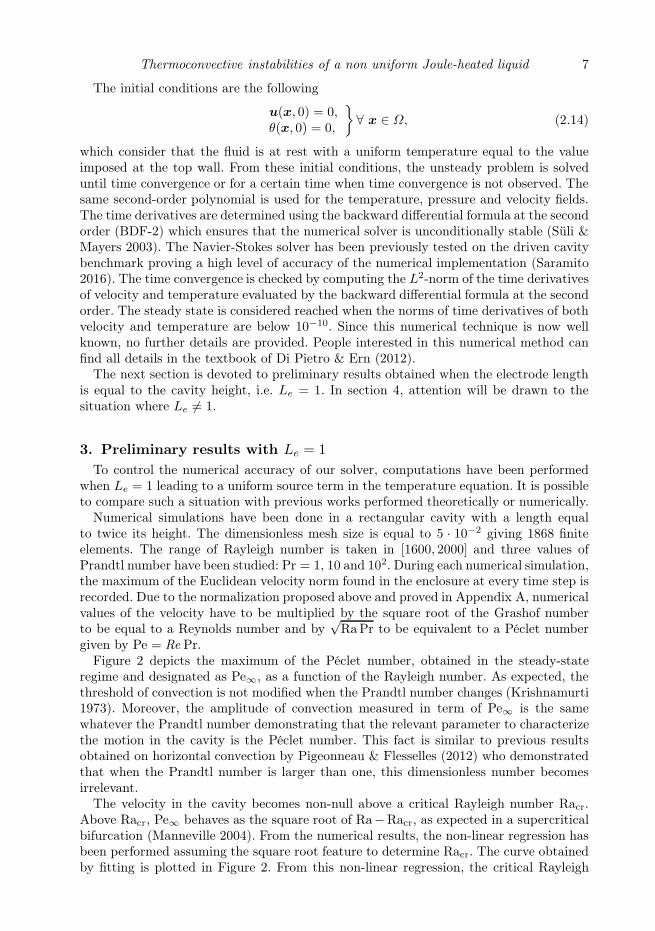
given by Pe = Re Pr.Figure 2 depicts the maximum of the Péclet number, obtained in the steady-state

regime and designated as Pe∞, as a function of the Rayleigh number. As expected, thethreshold of convection is not modified when the Prandtl number changes (Krishnamurti1973). Moreover, the amplitude of convection measured in term of Pe∞ is the samewhatever the Prandtl number demonstrating that the relevant parameter to characterizethe motion in the cavity is the Péclet number. This fact is similar to previous resultsobtained on horizontal convection by Pigeonneau & Flesselles (2012) who demonstratedthat when the Prandtl number is larger than one, this dimensionless number becomesirrelevant.

The velocity in the cavity becomes non-null above a critical Rayleigh number Racr.Above Racr, Pe∞ behaves as the square root of Ra−Racr, as expected in a supercriticalbifurcation (Manneville 2004). From the numerical results, the non-linear regression hasbeen performed assuming the square root feature to determine Racr. The curve obtainedby fitting is plotted in Figure 2. From this non-linear regression, the critical Rayleigh


1650 1700 1750 1800 1850 1900 1950 20000

0.5

1

1.5

2

2.5

3

3.5

4

Pe ∞

Ra

Pr = 1Pr = 10Pr = 102

Pe∞ = 2.086 · 10−1√

Ra−1702

Figure 2: Pe∞ as a function of Ra for L = 2, Le = 1 and Pr = 1, 10 and 100 obtainedwith a mesh size equal to h = 5 · 10−2.

number has been found to be 1702. To control the spatial resolution, we performed thesame numerical computations for Pr = 1 with a mesh size equal to 2.5 ·10−2, giving 7394finite elements. We do not observe any difference from the previous spatial resolution onRacr. Our critical Rayleigh number is larger than the solution given for a linear stabilityachieved in a periodic domain without vertical walls, for which Kulacki & Goldstein(1975) found a critical Rayleigh number equal to 1386. The finite domain and the no-slipboundary condition at each wall constrain the fluid to be at rest. Consequently, it isexpected to find a larger threshold value. The critical Rayleigh number obtained here isclose to the value determined numerically by Sugilal et al. (2005) in the same geometryand conditions. These authors employed a finite volume method with a uniform meshsize equal to 1/60 in both the space directions. They found a critical Rayleigh numberequal to 1650. Nevertheless, no effort was made to study the mesh convergence in thatcontribution.

Figure 3 plots the time behavior of the Reynolds number divided by the steady-statevalue for four Rayleigh numbers larger than the critical value in an enclosure of aspectratio equal to 2. The mesh size is h = 5 · 10−2 and the Prandtl number is equal to one.As expected in the case of a supercritical bifurcation, after an exponential growth, theamplitude of the velocity reaches the steady-state limit.

This kind of behavior can be described by the following equation (Manneville 2004)

Re

Re∞

=αeβrt√

1 + α2e2βrt, (3.1)

for which α and β are two constants of integration and the reduced control parameter ris defined by

r =Ra−Racr

Racr. (3.2)

The solid line in Figure 3 corresponds to this solution with α = 5.71·10−7 and β = 10.295.Figure 4 depicts the temperature field obtained for Ra = 1700, 1800, 1900 and for

Pr = 1. The temperature increases from the top to the bottom in the temperature range[0, 1] which does not change significantly for the three values of Ra meaning that the


0 0.25 0.5 0.75 1 1.25 1.5 1.75 2 2.25 2.510

-6

10-5

10-4

10-3

10-2

10-1

100

Re/Re∞

rt

Ra = 1775Ra = 1800Ra = 1825Ra = 1850Eq. (3.1)

Figure 3: Re/Re∞ as a function of rt for L = 2, Le = 1, Pr = 1 and for four Rayleighnumbers larger than the critical value.

(a) Ra = 1700 (b) Ra = 1800 (c) Ra = 1900

Figure 4: Isolines of temperature field in the enclosure for L = 2, Le = 1 and Pr = 1 witha mesh size h = 5 ·10−2 at (a) Ra = 1700, (b) Ra = 1800 and (b) Ra = 1900. Ten isolinesequally spaced between 0 (on the top boundary) and 1 (on the bottom boundary) havebeen drawn on each sub-figures.

values of isolines in Figure 4 are equivalent between the three solutions. At Ra = 1700which is just below the critical Rayleigh number established above, the fluid is at restand the temperature is expected to be in agreement with a simple solution of a pureheat diffusion equation given by Eq. (A 2) recalled in Appendix A. Above the criticalRayleigh number, the temperature field is advected by fluid motion. In our solution, thevelocity field is structured in two cells with a clockwise rotation for the left cell and ananticlockwise rotation for the right cell as shown in Figure 5. The maximum norm ofthe velocity is localized exactly in the middle of the enclosure and its value is equal to6.7 · 10−2. The two cell centres are on the line y = 1/2 with a localization at x = 0.575for the left cell and x = 1.425 for the right cell.

It is noteworthy that the sense of rotation of the two cells is arbitrary and comesfrom the numerical perturbations that arise, for instance, from small mesh anisotropy.Theoretically, both directions of rotation are possible. To examine this point, a numericalsimulation has been performed starting from the reverse of the steady-state solutionobtained at Ra = 1900 presented in Figure 5. The steady-state solution of this secondrun is shown in Figure 6 in which anticlockwise-clockwise cells are obtained. Whereasfrom the first solution, the Reynolds number obtained in the steady-state regime isequal to 2.92, the second solution gives a value equal to 2.76 showing that it is not


Figure 5: Velocity field in the enclosure for L = 2, Le = 1 and Pr = 1 with a mesh sizeh = 5 · 10−2 at Ra = 1900.

(a) Temperature (b) Velocity

Figure 6: Steady-state solution with anticlockwise-clockwise cells obtained by reversingthe solution with clockwise-anticlockwise cells for Ra = 1900. In sub-figure (a) tentemperature isolines are equally spaced between 0 (on the top boundary) and 1 (onthe bottom boundary).

purely the reverse of the first solution. This is due to the fact that the flow solutiondepends on the thermal features. Temperature isolines of this second solution depictedin figure 6a show that temperature is advected in the opposite direction in comparisonto the solution given in figure 4c. Due to the boundary conditions on θ between thebottom and top walls, up and down symmetry does not exist. The same observationhas been underlined by Bergeon et al. (1998) who investigated Marangoni convection.Consequently, the bifurcation observed here should be a transcritical bifurcation for whichone branch of the solution is supercritical and the second branch is subcritical.

In classical Rayleigh-Bénard convection, the thermal flux on boundaries where thetemperature is imposed is usually taken to define the Nusselt number. Here, due to thepresence of the source term and the energy conservation, the thermal gradient integratedover the top boundary is imposed and can not be used to define the Nusselt number.According to Roberts (1967) and Thirlby (1970) (see also (Goluskin 2016)), the averagetemperature over the cavity length is introduced as follows

〈θ〉(y, t) = 1

L

∫ L

0

θ(x, y, t)dx. (3.3)

The Nusselt number is seen as the ratio of the average temperature at the bottom wallwithout convection to the average temperature at the same location with convection.Since for a uniform volume source term, the temperature at the bottom wall is equal to


1650 1700 1750 1800 1850 1900 1950 20001

1.02

1.04

1.06

1.08

1.1

Nu

Ra

Pr = 1Pr = 10Pr = 100Nu = Ra / [Ra−0.585(Ra−Racr)]Nu = Ra / [Ra−0.599(Ra−Racr)]

Figure 7: Nu as a function of Ra for L = 2, Le = 1 and Pr = 1, 10 and 100 obtainedwith a mesh size equal to h = 2.5 · 10−2.

one, the Nusselt number is defined by

Nu =1

〈θ〉(0, t) . (3.4)

Figure 7 plots the Nusselt number as a function of Rayleigh number for three Prandtlnumbers. Below Racr, the Nusselt number is obviously equal to one since the fluid is atrest. Above Racr, Nu behaves quasi-linearly with Ra. The increase of the Nusselt numberis due to the decrease of the average temperature produced by the fluid motion. This isthe main signature of this case in which, when fluid motion occurs, the temperature inthe enclosure becomes more and more homogeneous with a decrease in the amplitude ofthe temperature range. More accurately, Thirlby (1970) proposed to describe the Nusseltnumber as follows

Nu =Ra

Ra−Γ (Ra−Racr), (3.5)

in which the coefficient Γ can be determined from the linear stability. Using the predictionof Roberts (1967), Thirlby (1970) gave a value for Γ = 0.599. From our numerical resultsobtained with three values of the Prandtl number, a regression computation gives a valueof Γ = 0.585. The solution obtained by the law given by Eq. (3.5) is provided as a solidline. To compare with the linear stability solution, we plot in Figure 7 the solution ofThirlby (1970) with Γ = 0.599 showing that the two laws are close even if in our casethe problem is described in a finite domain.

These preliminary results show that our numerical method is very accurate in describ-ing natural convection with a volumetric source term. The bifurcation occurring in thisconfiguration has been very well reproduced in agreement with the theoretical predictionsalready published. Now, we turn our attention to the situation where Le 6= 1 which isseldom studied.


Figure 8: Joule dissipation corresponding to 2L2(∇Φ)2 in the enclosure for Le = 2/3drawn over 16 colors equally ranged in [0; 5].

4. Convective regimes and transitions for Le 6= 1

From the practical point of view, electrodes are often shorter than the height of theenclosure. To study the effect of shortening of the electrodes, numerical simulations havebeen performed by cutting electrodes symmetrically from the bottom of the enclosure.

4.1. Onset of convection for Le < 1

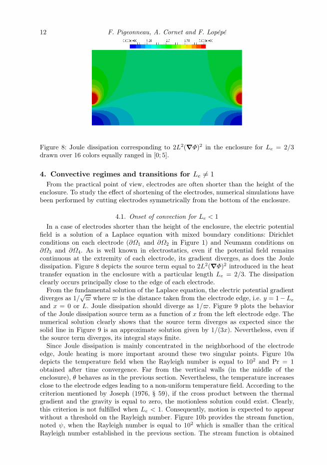
In a case of electrodes shorter than the height of the enclosure, the electric potentialfield is a solution of a Laplace equation with mixed boundary conditions: Dirichletconditions on each electrode (∂Ω1 and ∂Ω2 in Figure 1) and Neumann conditions on∂Ω3 and ∂Ω4. As is well known in electrostatics, even if the potential field remainscontinuous at the extremity of each electrode, its gradient diverges, as does the Jouledissipation. Figure 8 depicts the source term equal to 2L2(∇Φ)2 introduced in the heattransfer equation in the enclosure with a particular length Le = 2/3. The dissipationclearly occurs principally close to the edge of each electrode.

From the fundamental solution of the Laplace equation, the electric potential gradientdiverges as 1/

√ where is the distance taken from the electrode edge, i.e. y = 1−Le

and x = 0 or L. Joule dissipation should diverge as 1/. Figure 9 plots the behaviorof the Joule dissipation source term as a function of x from the left electrode edge. Thenumerical solution clearly shows that the source term diverges as expected since thesolid line in Figure 9 is an approximate solution given by 1/(3x). Nevertheless, even ifthe source term diverges, its integral stays finite.

Since Joule dissipation is mainly concentrated in the neighborhood of the electrodeedge, Joule heating is more important around these two singular points. Figure 10adepicts the temperature field when the Rayleigh number is equal to 102 and Pr = 1obtained after time convergence. Far from the vertical walls (in the middle of theenclosure), θ behaves as in the previous section. Nevertheless, the temperature increasesclose to the electrode edges leading to a non-uniform temperature field. According to thecriterion mentioned by Joseph (1976, § 59), if the cross product between the thermalgradient and the gravity is equal to zero, the motionless solution could exist. Clearly,this criterion is not fulfilled when Le < 1. Consequently, motion is expected to appearwithout a threshold on the Rayleigh number. Figure 10b provides the stream function,noted ψ, when the Rayleigh number is equal to 102 which is smaller than the criticalRayleigh number established in the previous section. The stream function is obtained


0 0.05 0.1 0.15 0.2 0.25 0.3 0.35 0.4 0.45 0.50

10

20

30

40

50

60

x

2L

2(∇

Φ)2

Num. sol.2L2(∇Φ)2 = 1/(3x)

Figure 9: Joule dissipation source term 2L2(∇Φ)2 as a function of x from the left electrodeedge, i.e. x = (0, 1− Le) in the enclosure for Le = 2/3.

(a) Temperature(b) Stream function

ψ = −9.55 · 10−4 ψ = 9.55 · 10−4

Figure 10: Temperature θ ∈ [0, 0.84] (drawn over 16 colors equally spaced) and streamfunction ψ obtained after time convergence for Pr = 1, Ra = 102 and Le = 2/3. Streamisolines are equally spaced over 30 values ranged in [−9.55 · 10−4; 9.55 · 10−4].

by solving a Poisson equation with a source term equal to the opposite of the vorticity.On the boundary, ψ is imposed equal to zero. An arrow has been added in Figure 10bto indicate the direction of the flow in the middle of the enclosure. Moreover, the valuesof ψ are given close to the cell centers in Figure 10b. The sign of ψ pinpoints therotation direction of cells which are clockwise and anticlockwise for the left and rightcells respectively, noting that this result is not a particular branch of solutions. Indeed,the vorticity direction results from the cross product ∇θ × ey, as can be easily verifiedby taking the rotational of the momentum equation (2.9). The direction of the thermalgradient in the neighborhood of the electrode edges being from the middle of the cavitytoward the vertical walls, the rotation directions of the left and right cells are necessarilyclockwise and anticlockwise respectively.

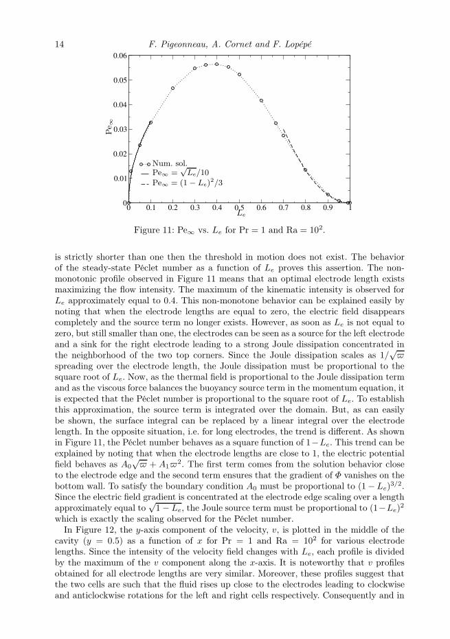
To study the nature of the transition when the electrode length changes, numericalcomputations have been done for Le ∈]0, 1[. The Prandtl number is set equal to 1 andthe Rayleigh number is equal to 102. As shown in Figure 11, when the electrode length


0 0.1 0.2 0.3 0.4 0.5 0.6 0.7 0.8 0.9 10

0.01

0.02

0.03

0.04

0.05

0.06

Pe ∞

Le

Num. sol.Pe∞ =

√Le/10

Pe∞ = (1− Le)2/3

Figure 11: Pe∞ vs. Le for Pr = 1 and Ra = 102.

is strictly shorter than one then the threshold in motion does not exist. The behaviorof the steady-state Péclet number as a function of Le proves this assertion. The non-monotonic profile observed in Figure 11 means that an optimal electrode length existsmaximizing the flow intensity. The maximum of the kinematic intensity is observed forLe approximately equal to 0.4. This non-monotone behavior can be explained easily bynoting that when the electrode lengths are equal to zero, the electric field disappearscompletely and the source term no longer exists. However, as soon as Le is not equal tozero, but still smaller than one, the electrodes can be seen as a source for the left electrodeand a sink for the right electrode leading to a strong Joule dissipation concentrated inthe neighborhood of the two top corners. Since the Joule dissipation scales as 1/

√

spreading over the electrode length, the Joule dissipation must be proportional to thesquare root of Le. Now, as the thermal field is proportional to the Joule dissipation termand as the viscous force balances the buoyancy source term in the momentum equation, itis expected that the Péclet number is proportional to the square root of Le. To establishthis approximation, the source term is integrated over the domain. But, as can easilybe shown, the surface integral can be replaced by a linear integral over the electrodelength. In the opposite situation, i.e. for long electrodes, the trend is different. As shownin Figure 11, the Péclet number behaves as a square function of 1−Le. This trend can beexplained by noting that when the electrode lengths are close to 1, the electric potentialfield behaves as A0

√ + A1

2. The first term comes from the solution behavior closeto the electrode edge and the second term ensures that the gradient of Φ vanishes on thebottom wall. To satisfy the boundary condition A0 must be proportional to (1− Le)

3/2.Since the electric field gradient is concentrated at the electrode edge scaling over a lengthapproximately equal to

√1− Le, the Joule source term must be proportional to (1−Le)

2

which is exactly the scaling observed for the Péclet number.In Figure 12, the y-axis component of the velocity, v, is plotted in the middle of the

cavity (y = 0.5) as a function of x for Pr = 1 and Ra = 102 for various electrodelengths. Since the intensity of the velocity field changes with Le, each profile is dividedby the maximum of the v component along the x-axis. It is noteworthy that v profilesobtained for all electrode lengths are very similar. Moreover, these profiles suggest thatthe two cells are such that the fluid rises up close to the electrodes leading to clockwiseand anticlockwise rotations for the left and right cells respectively. Consequently and in


0 0.25 0.5 0.75 1 1.25 1.5 1.75 2

-0.75

-0.5

-0.25

0

0.25

0.5

0.75

1

x

v/max(v)

Le = 0.01Le = 0.1Le = 0.3Le = 0.6Le = 0.9Le = 0.99

Figure 12: v/max(v) vs. x for Pr = 1 and Ra = 102 for various Le plotted for y = 0.5.

0 0.1 0.2 0.3 0.4 0.5 0.6 0.7 0.8 0.9 10

10

20

30

40

50

60

70

80

90

100

Pe ∞

Le

Ra = 104

Ra = 105

Pe∞ = 61.66 4√Le

Pe∞ = 17.86√Le

Pe∞ = 98.03 − 37.95(1 − Le)

Pe∞ = 22.39 − 23.1(1 − Le)2

Figure 13: Pe∞ vs. Le in the situation where Ra = 104 or 105 and for Pr = 1.

perfect agreement with our explanation given above using Joseph’s criterion, only oneflow structure exists when Le becomes less than one.

To go further, two other cases have been investigated for Ra = 104 and Ra = 105

which are larger than the critical Rayleigh number of the previous section. The influenceof the electrode length is also investigated for Pr = 1. For all numerical simulations, asteady-state regime is established. Figure 13 plots the Péclet number obtained after timeconvergence versus Le. The behavior changes strongly in comparison with the previousresults obtained at Ra = 102. Indeed, the Péclet number increases monotonically withLe for a Rayleigh number equal to 104. Using the previous analysis about the scaling ofthe Joule dissipation term, approximate solutions have been established for small Le andwhen 1− Le ≪ 1. Since the Rayleigh number is above the critical Rayleigh number it isclearly found that the flow does not vanish when Le goes to one.


(a) Le = 0.8 (b) Le = 0.9

Figure 14: Temperature field obtained for Ra = 105, Pr = 1 and for (a) Le = 0.8 and (b)Le = 0.9. In sub-figure (a), θ ∈ [0; 0.39] is drawn with a map of 16 colors equally spacedand in sub-figure (b), θ ∈ [0; 0.36].

Numerical computations performed at Ra = 105 provide new results. First, the increaseof the Péclet number at small Le is sharper than the solution obtained at Ra = 104. Thisresult can be easily explained by noting that at large Rayleigh number, the flow is mainlydriven by inertia. In this case, the balance in the momentum equation is achieved betweenthe inertia term and the buoyancy source. Consequently, the velocity scales as the squareroot of temperature. Since the temperature is proportional to the Joule dissipation, itis expected that when the electrode length is small, the velocity and in consequence thePéclet number scales as Le to the power one fourth. The approximate solution given inFigure 13 shows that this trend is verified.

The Péclet number presents a discontinuity between Le = 0.8 and 0.9. When Le 6 0.8,the Péclet number increases quasi-linearly with the electrode length which once again canbe explained using the scaling of the Joule dissipation term and the fact that the flowis in the inertial regime. To explain the discontinuity above Le = 0.8, it is necessaryto explore the flow structures. The temperature field is plotted for Ra = 105, Pr = 1and when the electrode lengths are equal to Le = 0.8 and Le = 0.9 in Figure 14. Thetemperature field for Le = 0.8 (panel a) is mainly driven by the convective transfermeaning that the structure is composed by the down-flow in the middle of the enclosureas already seen when Ra = 102. For Le = 0.9 (panel b), the flow structure shifts toanother solution with up-flow in the middle of the cavity creating a plume. Even if thedown-flow structure is favored, the up-flow structure can be stable. This solution can beconsidered as a disconnected branch investigated in more detail by Torres et al. (2014).

In fact, we postpone careful analysis of the different structures to subsection 4.3 studiedfor a electrode length equal to 2/3. We will see that the up-flow structure giving rise toa plume is observed for small Prandtl number.

4.2. Steady-state convective regime for Le = 2/3

In this subsection, the electrode lengths are set equal to 2/3 and we investigate theeffect of the Rayleigh and Prandtl numbers on the heat and mass transfer. Results in thissection are limited in the case for which the time convergence occurs. It is numericallyobserved that the range of Rayleigh number having a steady-state solution decreaseswhen the Prandtl number increases. Figures 15 and 16 provide the temperature andthe stream function for Ra = 104 and 105, respectively. While the temperature field atRa = 102, depicted in the previous subsection (Figure 10), is close to the solution of apure heat diffusion regime, the advection becomes stronger and stronger at Ra = 104

and 105, to become a main contribution in the solution of the temperature field. When



ψ = −4.6 · 10−2 ψ = 4.6 · 10−2

Figure 15: (a) θ ∈ [0, 0.55] mapped over 16 colors equally spaced; (b) stream functionranged in ±4.6 · 10−2 plotted with 30 isolines equally spaced obtained after timeconvergence for Pr = 1, Ra = 104 and Le = 2/3.


ψ = −4.36 · 10−2 ψ = 4.36 · 10−2

Figure 16: (a) θ ∈ [0, 0.36] mapped over 16 colors equally spaced; (b) stream functionranged in ±4.36 · 10−2 plotted with 30 isolines equally spaced obtained after timeconvergence for Pr = 1, Ra = 105 and Le = 2/3.

the Rayleigh number is equal to 102 and 104, the centers of the two cells are located onthe horizontal median of the enclosure. For Ra = 105, the vortex centers go down andbecome closer. In this situation, the flow structure is composed by two counter-rotatingcells with the formation, in the middle of the enclosure, of a jet directed downwards.

This observation of the flow structure indicates that at least two flow regimes existin this problem, in agreement with the scaling analysis provided in Appendix A. Atlow Rayleigh number, the flow regime is driven by heat conduction, whereas when theRayleigh number is large, the temperature field is driven by convection.

Figure 17 represents the steady-state Péclet number as a function of the Rayleighnumber obtained for four Prandtl numbers. The two regimes are clearly established inFigure 17. When the Rayleigh number is smaller than 103, the Péclet number behaveslinearly as a function of Rayleigh number. The pre-factor of the law depends on the lengthof the electrodes following the results obtained in subsection 4.1. Above Ra = 103, thebehavior of Pe∞ changes towards a convective regime for which the Péclet number scalesas the square root of the Rayleigh number. The first regime is in perfect agreement withthe scaling established in Appendix A in which the Reynolds number is proportional tothe Grashof number implying that the Péclet number is linear with the Rayleigh number.

The second regime needs enlightenment. Indeed, if only the momentum equation


100

101

102

103

104

10510

-4

10-3

10-2

10-1

100

101

102

Pe ∞

Ra

Pr = 1Pr = 10Pr = 102

Pr = 103

Pe∞ = 3 · 10−4 RaPe∞ = 0.28

√Ra

Figure 17: Pe∞ as a function of Ra for L = 2, Le = 2/3 and Pr = 1, 10, 102 and 103

obtained with a mesh size equal to h = 2.5 · 10−2.

is considered, as it was done in the scaling analysis, the balance of the inertial andthe buoyancy forces predicts that the dimensionless velocity is constant meaning thatthe Reynolds number should be proportional to

√

Ra /Pr and consequently the Péclet

number should scale as√

RaPr which is not the case. To establish the right scaling, itis crucial to take into account the fact that the Prandtl number is larger than one. Inthis case, the inertia does not play a significant role in the momentum equation meaningthat the balance is once again achieved between the viscous and the buoyancy terms asfollows

u0 ∼√

Ra

Prθ0, (4.1)

in which u0 is the order of magnitude of the dimensionless velocity and θ0 the typical valueof the reduced temperature. From the energy equation, the balance at large Rayleigh andPrandtl numbers is given by the convective term and the Joule dissipation such as

u0θ0 ∼ S√RaPr

, (4.2)

with S an arbitrary constant. Using these two equations, u0 is inversely proportionalto the square root of the Prandtl number. Consequently, the Reynolds number scalesas

√Ra/Pr and the Péclet number becomes proportional to the square root of the

Rayleigh number as is the case in Figure 17. The two kinematic regimes are insensitiveto the Prandtl number as observed in Figure 17 since the Péclet number does not changesignificantly when the Prandtl number increases from 1 to 103.

As shown in Figure 10-(b), Figure 15-(b) and Figure 16-(b), the temperature rangebecomes narrower when the Rayleigh number increases. To be more accurate in terms ofthermal behavior, the average temperature given by Eq. (3.3) is depicted in Figure 18.Four Prandtl numbers have been investigated. The Rayleigh number ranges between 102

and 2.4 · 104 for Prandtl numbers larger than 1. The last value of Ra has been chosenin order to have a steady-state solution. For Pr = 1, the largest value of the Rayleighnumber is equal to 105. For the two small Rayleigh numbers, the average temperatureprofile over the y-axis is close to the solution without convection. A sharp difference


0

0.2

0.4

0.6

0.8

1

0 0.2 0.4 0.6 0.80

0.2

0.4

0.6

0.8

1

0 0.2 0.4 0.6 0.8

y

y

〈θ〉〈θ〉

(a) Pr = 1 (b) Pr = 10

(c) Pr = 102 (d) Pr = 103

Ra = 102

Ra = 103

Ra = 3 · 103

Ra = 104

Ra = 2.4 · 104

Ra = 105

Figure 18: x-axis average temperature profile (y vs. 〈θ〉) for (a) Pr = 1, (b) Pr = 10, (c)Pr = 102 and Pr = 103 and for various Rayleigh numbers ranging between 102 to 105 forL = 2 and Le = 2/3 obtained with a mesh size equal to h = 2.5 · 10−2.

occurs when the Rayleigh number is larger than 103. The temperature profile becomesincreasingly flat far away the top horizontal wall. It is noteworthy that the temperatureprofiles are very similar for the four Prandtl numbers.

The Nusselt number defined by eq. (3.4) has been plotted in Figure 19 as a functionof Ra and for the four Prandtl numbers already mentioned. Clearly, two regimes areidentified: for Ra less than 103, the Nusselt number is constant while for Ra above 103

the Nusselt number increases with respect to Ra. Notice that the Nusselt number in theconductive regime is larger due to the fact that without motion the temperature range isa little smaller when the electrode length is shorter than the cavity height, as can be seenin Figure 18. For Prandtl numbers equal to 10 to 103, the profiles are completely similarmeaning that the Prandtl number does not play a significant role. Moreover, a nonlinearfitting shows that the Nusselt number increases slowly with the Rayleigh number sincethe dependence is logarithmic as already pointed out by Sugilal et al. (2005). For aPrandtl number equal to one, the Nusselt number has been determined up to the limitover which the solution becomes unsteady. Even if the logarithmic behavior is depictedas well for Pr = 1, the slope changes.

The Péclet and the Nusselt numbers provided in this subsection have been reportedwhen a steady-state regime is obtained. Over a threshold in terms of Rayleigh numberdepending of the Prandtl number, the stationary state with the symmetrical structure isnot reached. The following two subsections are devoted to the study of these transitions.


100

101

102

103

104

105

1

1.5

2

2.5

3

3.5

Nu

Ra

Pr = 1Pr = 10Pr = 102

Pr = 103

Nu = −3.917 + 0.688 ln(Ra)

Figure 19: Nu as a function of Ra for L = 2, Le = 2/3 and Pr = 1, 10, 102 and 103

obtained with a mesh size equal to h = 2.5 · 10−2.

4.3. Break-up of the symmetric solution for Le = 2/3

To control the steady-state regime, the L2-norms of the time derivatives of the velocityand temperature fields with the backward differential formula at the second order aredetermined as a function of time. To improve the time resolution, the time step is setequal to 2 ·10−3. The typical behavior of the time derivative of the velocity field obtainedfor a particular Prandtl number equal to 10 is depicted in Figure 20. The Rayleighnumber ranges between 1.1 · 104 and 2.5 · 104. The computation is stopped either whenthe maximum of the time derivatives of velocity and temperature becomes less than10−10 or when a predefined time is reached. At small Rayleigh numbers, convergenceis quickly reached. Whatever the Rayleigh number, the time derivative of the velocitydecreases exponentially with time due to the convergence following eigenmodes of theNavier-Stokes-Fourier equations. At short times, the fastest mode predominates whileat long times when the largest modes have already converged only the smallest moderemains which corresponds to the second behavior seen in Figure 20. When the Rayleighnumber increases, the absolute value of the smallest eigenvalue decreases, requiring alonger time to observe convergence. The fastest mode does not change significantly withthe Rayleigh number as shown in Figure 20 where rates of convergence at short times arepractically identical whatever Ra. In contrast, the smallest mode depends strongly onthe Rayleigh number. These results mean that the time derivative of the velocity duringthe second step behaves as follows:

∂u(x, t)

∂t= A(x)eγt, (4.3)

in which the eigenvalue γ characterizes the time convergence. As depicted in Figure 20,below a critical value, γ is negative and when the Rayleigh number becomes larger thana threshold which is close to 2.5 · 104 for Pr = 10, γ becomes positive meaning that thesystem evolves toward another state. The critical Rayleigh number of this first transitionwill be designated Racr1 .

When the Prandtl number is equal to one, the occurrence of the transition differs. First,Racr1 is much larger and requires more numerical accuracy. To determine the critical


0 5 10 15 20 25 30 35 40 45 50 55 6010

-10

10-9

10-8

10-7

10-6

10-5

10-4

10-3

10-2

10-1

100

t

||∂u ∂t||

Ra = 1.1 · 104Ra = 1.3 · 104Ra = 1.2 · 104Ra = 1.7 · 104Ra = 1.9 · 104Ra = 2.1 · 104Ra = 2.3 · 104Ra = 2.5 · 104

Figure 20: L2-norm of the time derivative of the velocity in the cavity as a function oftime for L = 2, Le = 2/3 and Pr = 10 obtained with a mesh size equal to h = 2.5 · 10−2

and a time step equal to 2 · 10−3.

Rayleigh number we perform numerical simulations by increasing the spatial resolutionwith a mesh size equal to 1.76 · 10−2 which increases the number of finite elements by afactor of two. The time step is once again taken equal to 2 · 10−3. Figure 21 depicts theL2-norm of the time derivative of the velocity as a function of time for three Rayleighnumbers taken close to the threshold. The critical Rayleigh number Racr1 is between1.66 · 105 and 1.67 · 105 meaning that when the Prandtl number is equal to one, we cantake Racr1 = 1.665 · 105 with an uncertainty equal to 0.6 %. While for Pr = 10 two stepsare observed in the convergence toward the steady-state regime, only one step emergesfor Pr = 1, underlining that the spectrum of eigenvalues is narrower for Pr = 1 than fora larger Prandtl number.

When the Prandtl number is larger than one, the critical Rayleigh number is deter-mined by studying the behavior of the eigenvalue γ given in eq. (4.3). Due to a strongvariation of the critical Rayleigh number when Pr ∈ [1; 10], γ is investigated when thePrandtl number ranges between 2 and 103. The eigenvalue γ has been determined byfitting the time derivative with a decaying exponential function of time. Figure 22 depicts−γ as a function of Ra. For each Prandtl number, a quadratic function of Ra is found.For the smallest Prandtl numbers, the Rayleigh number for which γ becomes positiveis large while when the Prandtl number becomes larger than 10, profiles of −γ mergetoward a unique behavior meaning that the critical Rayleigh number does not changesignificantly.

To determine more accurately the value of Racr1 , each curve of −γ is fitted with aquadratic function of Ra. The value of Racr1 is determined by finding the zero value of−γ. The solid line with circle symbols given later in Figure 33 presents the first criticalRayleigh number Racr1 as a function of the Prandtl number in which the critical Rayleighnumber obtained for Pr = 1 has been added. Racr1 decreases strongly when Pr is in therange [1; 10]. As already mentioned when Pr = 1, the critical Rayleigh number Racr1 is1.665 · 105 while above Pr = 10, Racr1 is approximately equal to 2.5 · 104 and does notchange significantly for larger Prandtl numbers.

The thermal and kinematic structures shown in Figure 15 for Ra = 104 and Pr = 1


0 2 4 6 8 10 1210

-10

10-9

10-8

10-7

10-6

10-5

10-4

10-3

10-2

10-1

100

t

‖∂u ∂t‖

Ra = 1.64 · 105Ra = 1.66 · 105Ra = 1.67 · 105

Figure 21: L2-norm of the time derivative of the velocity in the cavity as a function oftime for L = 2, Le = 2/3 and Pr = 1 obtained with a mesh size equal to h = 1.76 · 10−2

and a time step equal to 2 · 10−3.

10000 20000 30000 40000 500000

0.25

0.5

0.75

1

1.25

1.5

1.75

2

2.25

Ra

−γ

Pr = 2Pr = 3Pr = 10Pr = 30Pr = 102

Pr = 3 · 102Pr = 103

Figure 22: Behavior of −γ as a function of Ra number for Pr ∈ [2; 103].

for which two counter-rotating cells are observed do not stay stable above the criticalRayleigh number Racr1 . This bifurcation can be seen by looking the behavior of the L2-norm of u as a function of time. A typical curve is given in Figure 23 when Ra = 3.5 ·104and Pr = 102 corresponding to a condition above the transition. After a fast increase,the velocity norm reaches a first plateau. When the time is larger than 13, the velocitydecreases to reach a second plateau.

The modification of the flow structure can be seen by looking the iso-values of thetemperature field shown in Figure 24 for which six snapshots have been reported. Forthe two first snapshots, the structures are symmetric obtained when the velocity reachesthe first plateau in Figure 23. The observation of the stream function at the same timesrepresented in Figure 25 allows us to see the flow structure. For the two first snapshots,the flow structure is characterized by two counter-rotating cells. While at small times the


0 2 4 6 8 10 12 14 16 18 200

0.005

0.01

0.015

0.02

0.025

0.03

‖u‖

t

Figure 23: L2-norm of u as a function of time obtained for Pr = 102 and Ra = 3.5 · 104for L = 2, and Le = 2/3.

(a) t = 9, θ ∈ [0; 0.40] (b) t = 10, θ ∈ [0; 0.41] (c) t = 11, θ ∈ [0; 0.41]

(d) t = 12, θ ∈ [0; 0.43] (e) t = 13, θ ∈ [0; 0.48] (f) t = 14, θ ∈ [0; 0.51]

Figure 24: Snapshots of 10 equally spaced isolines of θ obtained for Pr = 102 and Ra =3.5 · 104 when time is equal to (a) t = 9, (b) t = 10, (c) t = 11, (d) t = 12, (e) t = 13 and(f) t = 14.

temperature field is symmetric with respect to the middle vertical axis, the symmetry isbroken when time becomes larger than 11 which is in the range where the L2-norm ofthe velocity plotted in Figure 23 decreases. The stream function shows that the left-handcell becomes more and more important relative to the right-hand cell (see Figure 25).When the time is larger than 14, a steady-state asymmetric flow structure is observedwith only one cell.

The transition from the two symmetric cells to one asymmetric cell also has an effect onthe behavior of the Nusselt number. In Figure 26, the time behavior of Nu is plotted whenthe Rayleigh number is equal to 3.5 · 104 and Pr = 102. As for the norm of the velocityfield, two values of the Nusselt number arise. The first plateau is obtained when the flowstructure is composed by the two symmetric cells. After a fast transition obtained when


(a) t = 9, [−4.82; 4.82] · 10−3 (b) t = 10, [−4.86; 4.73] · 10−3 (c) t = 11, [−4.97; 4.60] · 10−3

(d) t = 12, [−5.20; 4.1] · 10−3 (e) t = 13, [−5.30; 2.29] · 10−3 (f) t = 14, [−5.46; 0.00] · 10−3

Figure 25: Snapshots of 10 equally spaced isolines of ψ obtained for Pr = 102 andRa = 3.5 · 104 when time is equal to (a) t = 9, (b) t = 10, (c) t = 11, (d) t = 12, (e)t = 13 and (f) t = 14. For each sub-figure, the range of ψ has been reported in eachsub-caption.

0 2 4 6 8 10 12 14 16 18 202.5

3

3.5

4

4.5

5

t

Nu

Figure 26: Nu as a function of time obtained for Pr = 102 and Ra = 3.5 · 104 for L = 2,and Le = 2/3.

t ∼ 13, the Nusselt number decreases by 13% to reach a second constant value when thesecond regime is fully established.

The asymmetric solution observed in sub-figures 24f and 25f is characterized by aclockwise cell. This rotation is chosen artificially by the solver. Indeed, due to the left-right symmetry, a solution with an anticlockwise rotation cell is totally possible. Froma previous converged solution, a numerical test with an initialized solution obtained bychanging x in L−x proves that the anticlockwise cell structure is also a solution meaningthat we found two branches of solutions respecting the symmetry of the problem.

Once again, the transition when the Prandtl number is equal to one is different. A


(a) t = 1.5, θ ∈ [0; 0.35] (b) t = 2, θ ∈ [0; 0.36] (c) t = 2.3, θ ∈ [0; 0.28]

(d) t = 2.6, θ ∈ [0; 0.27] (e) t = 3, θ ∈ [0; 0.32] (f) t = 3.6, θ ∈ [0; 0.32]

Figure 27: Snapshots of 10 equally spaced isolines of θ obtained for Pr = 1 and Ra =1.68 · 105 for (a) t = 1.5, (b) t = 2, (c) t = 2.3, (d) t = 2.6, (e) t = 3 and (f) t = 3.6.

numerical simulation has been made at Ra = 1.68 · 105. Figure 27 depicts six snapshotsof iso-values of θ. Starting from a symmetric structure relatively similar to the previousone observed at Pr = 100, the flow structure changes completely, as can be seen inFigure 27-(c). Two counter-rotating cells are present but with a change in rotation.Before the transition, the fluid moves up close to the vertical boundaries while at thetransition, the fluid moves down close to the vertical walls. After a period of transition,the flow is structured with two counter-rotating cells for which the fluid moves up in themiddle of the cavity leading to a creation of a plume. As seen in Figure 27-(f) obtained att = 3.6, the structure is quite symmetric which is not the case of the transition observedwhen the Prandtl number is larger than 3. The solution obtained for Pr = 1 is similar tothat reported by Sugilal et al. (2005).

It is noteworthy that when the Prandtl number is less than 3, the flow structurebecomes asymmetric over Racr1 as observed for larger Pr. Moreover, numerical solutionsperformed for larger Rayleigh numbers converge toward a steady-state structure similarto the one observed at Pr = 1. For a Prandtl number larger than 3, this transition is notobserved but the solution becomes unsteady, as will be shown in the next subsection.

4.4. Hopf bifurcation for large Ra and Pr > 10

Solutions found for (Ra = 3.5 · 104,Pr = 102) and (Ra = 1.68 · 105,Pr = 1) stay in asteady-state regime, since after the transition, the time convergence is numerically found.By increasing the Rayleigh number when Pr > 3, a second instability is established forwhich the solution becomes periodic in time. Using a simple dichotomy method, theonset of the second instability is determined. This second instability is characterized bya critical Rayleigh number Racr2 . Figure 33, given later, depicts the behavior of Racr2 asa function of Pr (solid line with square symbols).

To see the occurrence of the periodic solution, Figure 28 presents the behavior ofthe L2-norm of the velocity for four Rayleigh numbers when the Prandtl number isequal to 10. As already seen in Figure 23, the norm of the velocity rapidly reaches aplateau corresponding to the symmetric configuration followed by a decrease of the flowintensity. Figure 28 depicts the behavior after the first transition. The establishmentof the periodic solution depends on the gap between the Rayleigh number used fora particular computation and Racr2 . The transition occurs earlier when the Rayleigh


6 7 8 9 100.05

0.06

0.07

0.08

5 5.5 6 6.5 7

4.5 5 5.5 60.05

0.06

0.07

0.08

4 4.5 5

‖u‖

‖u‖

tt

(a) Ra = 4.5 · 104 (b) Ra = 5 · 104

(c) Ra = 5.5 · 104 (d) Ra = 6 · 104

Figure 28: ‖u‖ as a function of t for Pr = 10 and (a) Ra = 4.5 · 104, (b) Ra = 5 · 104, (c)Ra = 5.5 · 104 and (d) Ra = 6 · 104.

number increases. The periodic regime begins with an increase in the amplitude ofoscillations and its duration becomes shorter as Ra increases. Amplitudes of velocityoscillations grow with the Rayleigh number.

In order to see the effect of the second transition on the thermal structure, the Nusseltnumber is plotted as a function of time in Figure 29 when the Prandtl number is equal to10 and for four Rayleigh numbers equal to 4.5 ·104, 5 ·104, 5.5 ·104 and 6 ·104. As alreadymentioned above, the transition to the second instability occurs later when the Rayleighnumber is lightly larger than the critical Rayleigh number. The periodic solution doesnot lead to a strong effect on the Nusselt number. While the oscillation on the velocityis clearly observed when Ra = 4.5 · 104, the Nusselt number stays more and less stableabove the second transition. The amplitude of Nu increases for larger Rayleigh numbersbut the increase is very weak. We previously observed that the Nusselt number evolvesslowly with the Rayleigh number when Ra is smaller than Racr1 . Therefore, it is expectedto see a weak effect on heat transfer.

In order to show typical results, we provide a movie available at https://doi.org/10.1017/jfm.2018.168recording the temperature field determined when the Pr = 102 and Ra = 4 · 104. Fromthe initial condition for which the temperature is set equal to zero, the temperaturefield rapidly reaches the first regime corresponding to the symmetric condition. After acertain time, the flow moves to the asymmetric structure. Finally, the oscillations startto grow before reaching the periodic regime. The oscillations are mainly observed closeto the right vertical wall in the enclosure. Nevertheless, as already pointed out in theprevious subsection in which a steady-state one cell structure has been obtained, theperiodic solution with an anticlockwise cell can be obtained numerically. This meansthat once again two branches of solutions are possible.

Additional calculations have been made for Prandtl numbers equal to 10, 102 and


2 3 4 5 6 72.9

3

3.1

3.2

3.3

3.4

3.5

Nu

t

Ra = 4.5 · 104Ra = 5 · 104Ra = 5.5 · 104Ra = 6 · 104

Figure 29: Nu as a function of t for Pr = 10 and for Ra = 4.5 · 104, 5 · 104, 5.5 · 104 and6 · 104.

(a) Pr = 10

0 10 20 30 40 50 600

0.005

0.01

0.015

A

f

Ra = 4.5 · 104Ra = 5 · 104Ra = 5.5 · 104Ra = 6 · 104

(b) Pr = 102

0 10 20 30 40 50 600

0.001

0.002

0.003

0.004

f

Ra = 4 · 104Ra = 4.5 · 104Ra = 5 · 104Ra = 6 · 104

Figure 30: Fourier spectra of the norm of ‖u‖ for Pr = 10 and 102.

103 and for various Rayleigh numbers above Racr2 . In order to obtain more informationabout the nature of the second instability, a Fourier analysis has been performed in thetime range for which the flow is fully periodic. Figure 30 depicts the Fourier spectraobtained for two Prandtl numbers and four Rayleigh numbers. The amplitude and thefrequency are respectively designated by A and f . Signals are very close to a sinusoidalbehavior with a fundamental frequency and an amplitude corresponding to the velocityoscillation seen in Figure 28. Secondary peaks are observed at a frequency equal to asecond harmonic of the signal but with a much smaller amplitude.

From the asymmetric solution established when the Rayleigh number is above Racr1 ,the flow solution converges toward a limit cycle when Ra > Racr2 . The periodic solutionsobserved here look like a supercritical Hopf bifurcation which can be characterized by theamplitude and the frequency of oscillations (Manneville 2004). Using the Fourier analysis,the amplitude and the frequency of the fundamental harmonic can be determined. Asalready pointed out in § 4.2, the flow motion is very well described in terms of thePéclet number whatever the Prandtl number. In order to have an amplitude similar tothe Péclet number, the fundamental amplitude is multiplied by

√RaPr. According to


0 0.1 0.2 0.3 0.4 0.5 0.60

2

4

6

8

10

12

A√

RaPr

r

Pr = 10Pr = 102

Pr = 103

A√

RaPr = 13.053√r

Figure 31: Fundamental amplitude A√

Ra Pr as a function of the reduced controlparameter r for three Prandtl numbers.

Manneville (2004, pages 128-129), the oscillation amplitude is a function of the reducedcontrol parameter r given for this second instability by

r =Ra−Racr2

Racr2. (4.4)

Figure 31 presents the fundamental amplitude multiplied by√

RaPr as a function of rfor Pr = 10, 102 and 103. Even if numerical results are little scattered meaning thatthe limits of our numerical resolutions are close, a clear trend is observed. A non-linearregression shows that the amplitude grows as the square root of r as expected in the Hopfbifurcation. Moreover, the fundamental frequency f plotted as a function of r providedin Figure 32 shows that f is a linear function of the reduced control parameter.

It is noteworthy that the periodic solution presents a master result whatever thePrandtl number which has important consequences for industrial applications. Moreover,when the Prandtl number is larger than 102, the critical Rayleigh numbers Racr1 andRacr2 do not depend on Pr. Consequently, only the Rayleigh number remains as a controlparameter of the flow.

4.5. Stability diagram

A summary of the four main structures obtained for the specific electrode length Le =2/3 is provided in Figure 33. Below the curve giving Racr1 , the flow is composed of aunique symmetric structure with a left clockwise cell and a right anticlockwise cell. Thefluid goes from the top to the bottom in the middle of the enclosure. In this regime, thePéclet number is a linear function of Ra when Ra < 103 and a square root function ofRa when Ra > 103. Above the first critical Rayleigh number, an asymmetric structure isobserved for which anticlockwise or clockwise cells are obtained. The characteristic of thetransition between symmetric/asymmetric solutions is hard to establish with our timeintegration method. A stability study would be needed to explain why the symmetricsolution does not stay stable. Nevertheless, the base solution is hard to extract to performa stability analysis. Physically, the mechanism of the destabilization would be due to


0 0.1 0.2 0.3 0.4 0.5 0.6

22

24

26

28

30

f

r

Pr = 10Pr = 102

Pr = 103

f = 22.32 + 12.45r

Figure 32: Fundamental frequency f as a function of the reduced control parameter r forthree Prandtl numbers.

the instability of the central jet. Indeed, if the jet shifts a little horizontally then adisequilibrium in pressure occurs pushing the jet toward the side where the jet is shifted.

Below a Prandtl number equal to 3 and above a second critical Rayleigh number, athird flow structure is observed characterized by a left anticlockwise cell and a rightclockwise cell leading to vertical flow in the middle of the enclosure. Finally when thePrandtl number is larger than 3 and for Ra > Racr2 , an unsteady asymmetric structurearises. Due to left-right symmetry of the problem, two branches of solutions with anti-and clockwise cells exist.

4.6. Consequences for electric glass melting

Results obtained may have important consequences for the glass melting process. First,the occurrence of asymmetric structures can lead to a disequilibrium of the electric circuitand of the fusion of raw materials. When the flow structure shifts from a symmetricstructure to an asymmetric situation for which hot spots are observed close to electrodes,the raw materials can disappear and the thermal insulation is strongly affected. Moreover,electrodes can be eroded strongly. Unsteady solutions can also be a source of processinstabilities difficult to control for glass makers.

From the linear regression given in Figure 32, the dimensionless frequency is larger than22.32. In order to have an idea concerning the value of this frequency in SI units, thedimensionless frequency has to be multiplied by κ/H2. Since the typical height in glassmelting industry is approximately one meter, only the value of the thermal diffusivity isrequired. As already mentioned in the introduction and in § 2, radiation is the main modeof thermal transfer. Using a simple Rosseland approximation, the thermal conductivityis given by (Viskanta & Anderson 1975)

λ =16n2σSBT

3

3βR, (4.5)

with n is the refractive index typically equal to 1.5 for glass former liquids, σSB isthe Stefan-Boltzmann constant equal to 5.67 · 10−8 W·m−2·K−4, T is the absolutetemperature and βR is the Rosseland absorption coefficient given in m−1. For the typical


100

101

102

10310

4

105

Ra

Pr

Symmetric steady-state cells

Asymmetric steady-state anti- or clockwise cell

Steady-state cells

Racr1

Racr2

Asymmetric unsteady anti- or clockwise cell

Figure 33: Stability diagram (Pr,Racr1,2) describing the three main structures obtainednumerically when Le = 2/3. The first transition is delimited by Racr1 given in solid linewith circle symbols. The second transition is given by Racr2 in solid line with squaresymbols.

glass composition used to make wool insulation, the Rosseland absorption coefficient isequal to 200 m−1. Since the thermal diffusivity is given by λ/(ρCp) and if the temperatureis taken equal to 1300C, κ is approximately 3 · 10−6 m2·s−1. Using the dimensionlessfrequency equal to 22.23, we found that oscillations occur at 3 · 10−4 Hz correspondingto a time period of approximately one hour. For a dark glass, the Rosseland absorptioncoefficient is much larger and is typically equal to 1000 m−1 giving a smaller oscillationfrequency of approximately 6 · 10−5 Hz (time period close to 5 h).

5. Conclusion

This work has been devoted to natural convection in a Joule-heated cavity. A non-uniform volumetric heat source is produced by an electric field applied with two verticalelectrodes localized on the vertical walls of the enclosure. The coupled Navier-Stokes, heattransfer and electric potential equations are solved using a discontinuous Galerkin finiteelement technique. The solver is tested in a situation for which the heat source is uniformin volume leading to a threshold in convection similar to in classical Rayleigh-Bénardconvection. The critical Rayleigh number is determined. The bifurcation is similar to atranscritical one for which two solutions are possible. The heat transfer is characterizedby computing the average temperature profile over the horizontal coordinate.

After this preliminary test validating the numerical solver, we shorten the electrodesfrom the bottom. In such a case, the threshold disappears and the flow exists as soon


as the Rayleigh number is larger than zero. By studying the full range of the electrodelength, an optimal length has been obtained when the Rayleigh number is less than 1702.

Numerical simulations have been made for a large range of Prandtl number, between1 to 103 and a large range of Rayleigh number, up to 105 limited at only one electrodelength set equal to 2/3 of the cavity height. This case presents a large possibility ofsolutions starting from a symmetric two-cell steady-state with two rotation directions,an asymmetric cell steady-state and finally asymmetric cell time-periodic solutions. Inthe first kind of solution, the intensity of convection can be characterized in terms of thePéclet number. Two regimes arise: one obtained when the Rayleigh number is smallerthan 103, exhibiting a linear behavior of the Péclet number versus the Rayleigh number;the second regime is characterized by a square root dependency of the Péclet number asa function of Rayleigh number.

On increasing the Rayleigh number, the flow does not remain in the symmetricstructure. Using the behavior of the convergence toward the steady-state regime, weestablish the behavior of the critical Rayleigh number as a function of the Prandtl numberof this first transition. At small Prandtl number, the dependency on the critical Rayleighnumber is very important. However, when the Prandtl number is larger than 10, thecritical Rayleigh number does not change significantly and is equal to 2.5 · 104.

This second solution becomes periodic in time above a second critical Rayleigh numberwhich is less sensitive to the Prandtl number. Performing numerical simulations forRayleigh numbers above the second critical Rayleigh number allows us to quantify theamplitudes and frequencies of the observed oscillations. We prove that the nature ofthe second instability is a supercritical Hopf bifurcation. A stability diagram has beenestablished. Even though one electrode length has been investigated, it is expected thatwith another electrode length the critical Rayleigh numbers will change. However thevarious solutions established in this work should be the same.

In terms of industrial processes, the occurrence of a periodic flow can be a source ofdifficulties in controlling industrial plants. In the glass industry, the typical Rayleighnumber is always larger than the critical value found in the present study. Moreover,we observe that the flow structure can change dramatically which can be deleterious forworking conditions. Conversely, these instabilities could be an opportunity to control theheat and mass transfer since we establish a simple relation between oscillating solutionsand the Rayleigh number. The purpose here should be to improve the homogeneizationprocess, which is very important in applications because the forming process is mainlycontrolled by the thermal and chemical homogeneities of the glass former liquid at theexit of the furnace.

Even if careful attention has been paid to obtain good numerical accuracy, our solutionshave a limit in terms of space and time resolutions. Due to the large range of possiblesolutions and the dependence on up to three parameters, a continuation method wouldbe more appropriate to explore the stability of this kind of problem. Moreover, our studyfocuses only on two-dimensional configurations and only one length of electrode has beeninvestigated. To examine whether such instabilities are also present in more realisticsituations, we plan to extend this work to three-dimensional numerical simulations inthe near future.

Acknowledgements

The authors would like to thank Michael J. Toplis (IRAP, Toulouse) for his help in thepreparation of the article. We are also indebted to anonymous referees for perspicacious


comments and suggestions in the structure of this article which strongly improved itsquality.

Supplementary movie

Supplementary movie is available at https://doi.org/10.1017/jfm.2018.168.

Appendix A. Scaling analysis

In the problem statement, the set of conservative equations are normalized by charac-teristic quantities justified by a scaling analysis provided in this appendix.

A.1. Temperature scale

The scale of temperature range can be established by studying the solution withoutmotion. Indeed, when the electric potential is applied on the entire vertical boundary,i.e. Le = H , Φ is given by the following linear relation

Φ = Φ0

(

1− x

L

)

. (A 1)

With this electric field, the temperature without motion can also be found easily. Itssolution is

T = T0 +σΦ2

0H2

2λL2

(

1− y2

H2

)

. (A 2)

With this solution, the difference of temperature can be defined as follows:

∆T =σΦ2

0H2

2λL2, (A 3)

which arises from the balance between thermal conduction and Joule dissipation.When the electrode length is smaller than H , the electric field is no longer a linear

function of x and the accurate solution must be determined numerically. As it pointedout in § 4, Φ exhibits strong variations close to electrodes. However, outside the verticalwalls, the electric potential is quasi-linear meaning that the Joule dissipation source isapproximately uniform. The range of temperature does not change significantly and theprevious estimation can be applied. With such a scaling, the temperature can be writtenin the following dimensionless form:

θ =T − T0∆T

. (A 4)

Note that when Le = H , the thermal field is independent of x and is thermally unstable.

A.2. Velocity scale

The space coordinates are normalized with the height of the enclosure, H . Beforestudying the scaling of the velocity, the dimensionless forms of the potential Φ, and J

have to be defined. It is obvious that Φ is reduced by Φ0. Following Ohm’s law,

J = −σ∇Φ, (A 5)

where J is normalized by σΦ0/H .The velocity field is normalized by a scale U , the time by τ and the pressure by δP .

In the following, all dimensionless variables are written with the same symbols alreadyintroduced so that no misunderstanding is possible.


It is noteworthy that due to the fact that the pressure gradient must be kept in themomentum equation in order to satisfy the continuity equation, δP is on the order ofρgβ∆TH . Reporting these scalings in the momentum equation gives the general form ofthe momentum equation

Re

(

St∂u

∂t+ u ·∇u

)

= −∇p+∇2u+

Gr

Reθey, (A 6)

for which the dimensionless numbers are the following

Re =UH

ν: Reynolds number, (A 7)

St =H

τU: Strouhal number, (A 8)

Gr =gβ∆TH3

ν2: Grashof number, (A 9)

and ν = η/ρ is the kinematic viscosity. Recall that the Reynolds number is the ratio ofthe inertial to viscous forces. The Strouhal number which will be examined in the nextsubsection compares the relevant time scale of the dynamics to the advection time overthe height of the cavity. The Grashof number is a relevant number when buoyancy forcesare involved in the dynamics. It can be seen as the ratio of the momentum diffusion timeto advection time due to buoyancy forces. Recall that the Grashof number can be givenas a function of two other classical numbers as follows

Gr =Ra

Pr, (A 10)

with Ra the Rayleigh number and Pr the Prandtl number defined by eqs. (2.12) and(2.13) respectively.

Two main scenarii appear as a function of the Reynolds number. First, if Re is assumedsmall, a balance force is achieved between the viscosity and buoyancy effects leading tothe following scaling of the Reynolds number:

Re = Gr . (A 11)

In such a situation, the velocity scale U is proportional to β∆TgH2/ν. Conversely, ifthe inertia is important, the balance is achieved between inertial and buoyancy terms.Consequently, the Reynolds number behaves as

Re =√

Gr, (A 12)

leading to the order of magnitude of U being equal to√β∆TgH.

A.3. Time scale

The time scale is given by the amplitude of the Strouhal number. Since two types oftransfer occur in this problem, i.e. momentum and heat, the dynamics is controlled by theslowest phenomena. In order to establish the order of magnitude of the Strouhal number,the thermal equation can be rewritten in a dimensionless form using the previous scalingas follows

St∂θ

∂t+∇θ · u =

1

Pr Re

[

∇2θ + 2L2 (∇Φ)

2]

. (A 13)

Recall here the length L is the dimensionless length.By using the dimensionless momentum equation (A 6) and assuming that the Reynolds


number is larger than one, the Strouhal number can be scaled by

St = min

(

1

Re,

1

PrRe

)

, (A 14)

for which two limit cases arise as a function of the Prandtl number. Since in the frameworkof this study the Prandtl number is considered larger than one, the Strouhal number isgiven by

St =1

PrRe, (A 15)

meaning that the time scale is controlled by the thermal diffusion for which the typicaltime scale is τ = H2/κ.

To solve numerically the coupled Navier-Stokes-Fourier equations, the velocity scaleis taken in the limit of large Reynolds number meaning that this dimensionless numberis the square root of the Grashof number. This choice has been done because when theGrashof number is large the buoyancy term becomes important. By taking Re =

√Gr,

a better balance of the various terms in the momentum equation is obtained since theconvective and buoyancy terms are of the same order of magnitude.

Following these developments, the momentum and thermal partial differential equa-tions can be written as follows

1

Pr

∂u

∂t+

√

Ra

Pru ·∇u = −∇p+∇

2u+

√

Ra

Prθey, (A 16)

∂θ

∂t+√

Pr Ra∇θ · u = ∇2θ + 2L2 (∇Φ)

2, (A 17)

meaning that the momentum equation is quasi-steady when Pr ≫ 1.

REFERENCES

Batchelor, G. K. 1954 Heat tranfert by free convection across a closed cavity between verticalboundaries at different temperatures. Quart. Appl. Math. 12, 209–233.

Bergeon, A., Henry, D., Behadid, H. & Tuckerman, L. S. 1998 Marangoni convectionin binary mixtures with Soret effect. J. Fluid Mech. 375, 143–177.

Chiu-Webster, S., Hinch, E. J. & Lister, J. R. 2008 Very viscous horizontal convection.J. Fluid Mech. 611, 395–426.

Choudhary, M. K. 1986 A three-dimensional mathematical model for flow and heat transferin electrical glass furnaces. IEEE Trans. Ind. Appl. IA-22 (5), 912–921.

Curran, R. L. 1971 Use of mathematical modeling in determining the effects of electrodeconfiguration on convection currents in an electric glass melter. IEEE Trans. Ind. Appl.IGA-7 (1), 116–129.

Curran, R. L. 1973 Mathematical model of an electric glass furnace: Effects of glass color andresistivity. IEEE Trans. Ind. Appl. IA-9 (3), 348–357.

Di Pietro, D. A. & Ern, A. 2012 Mathematical aspects of discontinuous Galerkin methods.Heidelberg: Springer-Verlag.

Emara, A. A. & Kulacki, F. A. 1980 A numerical investigation of thermal convection in aheat-generating fluid layer. J. Heat Transfer 102 (3), 531–537.

Flesselles, J.-M. & Pigeonneau, F. 2004 Kinematic regimes of convection at hight Prandtlnumber in a shallow cavity. C. R. Mécanique 332, 783–788.

Goluskin, D. 2016 Internally Heated Convection and Rayleigh-Bénard Convection. Springer.Gopalakrishnan, S., Thess, A., Weidmann, G. & Lange, U. 2010 Chaotic mixing in a

Joule-heated glass melt. Phys. Fluids 22 (1), 013101.Gramberg, H. J. J., Howell, P. D. & Ockendon, J. R. 2007 Convection by a horizontal

thermal gradient. J. Fluid Mech. 586, 41–57.Joseph, D. D. 1976 Stability of fluid motions II . Berlin: Springer-Verlag.


Krishnamurti, R. 1973 Some further studies on the transition to turbulent convection. J. FluidMech. 60 (02), 285–303.

Kulacki, F. A. & Goldstein, R. J. 1975 Hydrodynamic instability in fluid layers withuniform volumetric energy sources. Appl. Sci. Res. 31 (2), 81–109.

Manneville, P. 2004 Instabilities, Chaos and Turbulence. World Scientific PublishingCompany.

Pigeonneau, F. & Flesselles, J.-M. 2012 Practical laws for natural convection of viscousfluids heated from above in a shallow cavity. Int. J. Heat Mass Transfer 55, 436–442.

Roberts, P. H. 1967 Convection in horizontal layers with internal heat generation. theory. J.Fluid Mech. 30 (01), 33–49.

Ross, C. P. & Tincher, G. L. 2004 Glass Melting Technology: A Technical and EconomicAssessment . Werterville (OH, USA): Glass Manufacturing Industry Council.

Saramito, P. 2015a Efficient C++ finite element computing with Rheolef . CNRS-CCSD ed.Saramito, P. 2015b Efficient C++ finite element computing with Rheolef: vol. 2. Discontinuous

Galerkin methods. CNRS-CCSD ed.Saramito, P. 2016 Complex fluids. Modeling and Algorithms, Mathématiques et Applications,

vol. 79. Springer.Scholze, H. 1990 Glass. Nature, Structures and Properties. Berlin: Springer-Verlag.Stanek, J. 1977 Electric melting of glass. Paris: Elsevier.Sugilal, G., Wattal, P. K. & Iyer, K. 2005 Convective behaviour of a uniformly Joule-

heated liquid pool in a rectangular cavity. Int. J. Therm. Sci. 44, 915–925.Süli, E. & Mayers, D. F. 2003 An Introduction to Numerical Analysis. Cambridge (UK):

Cambridge University Press.Thirlby, R. 1970 Convection in an internally heated layer. J. Fluid Mech. 44 (04), 673–693.Torres, J. F., Henry, D., Komiya, A. & Maruyama, S. 2014 Bifurcation analysis of steady

natural convection in a tilted cubical cavity with adiabatic sidewalls. J. Fluid Mech. 756,650–688.

Tritton, D. J. & Zarraga, M. N. 1967 Convection in horizontal layers with internal heatgeneration. experiments. J. Fluid Mech. 30 (01), 21–31.

Uguz, K. E., Labrosse, G., Narayanan, R. & Pigeonneau, F. 2014 From steady tounsteady 2-D horizontal convection at high Prandtl number. Int. J. Heat Mass Transfer71, 469–474.

de Vahl Davis, G. 1983 Natural convection of air in a square cavity: a bench mark numericalsolution. Int. J. Numer. Methods Fluids 3 (3), 249–264.

Viskanta, R. & Anderson, E. E. 1975 Heat transfer in semitransparent solids. Advances inheat transfer 11, 317–441.

Zeytounian, R. K. 2004 Theory and applications of viscous fluid flows. Berlin: Springer.

thermoconvective instabilities of a non uniform joule

Documents