Thermodynamics and life

Ilya Prigogine

1917 - 2003

Lectures on Medical Biophysics

Dept. Biophysics, Medical faculty, Masaryk University in Brno

Lecture outline

• Basic concepts of non-equilibrium thermodynamics of living systems

• Diffusion • Osmosis and osmotic pressure

Basic concepts of non-equilibrium thermodynamics of living systems

• There is an internal „source“ of entropy in non-equilibrium systems.

• The amount of entropy produced per unit volume in unit time is called the entropy production rate σ.

Prigogine principle

• For states not too far from tmd. equilibrium, the Prigogine principle applies:At constant external conditions, an open system spontaneously proceeds towards a state with a minimum entropy production rate.

• This state is called a stationary state (in biology: state of dynamic equilibrium, homeostasis respectively).

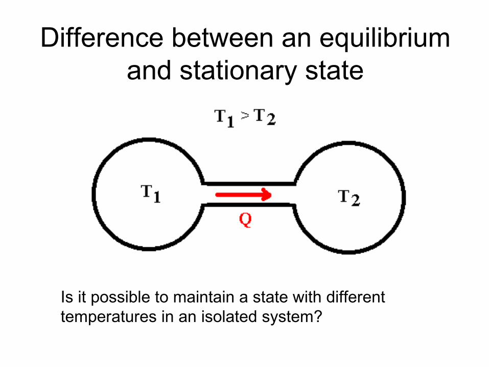
Difference between an equilibrium and stationary state

Is it possible to maintain a state with different temperatures in an isolated system?

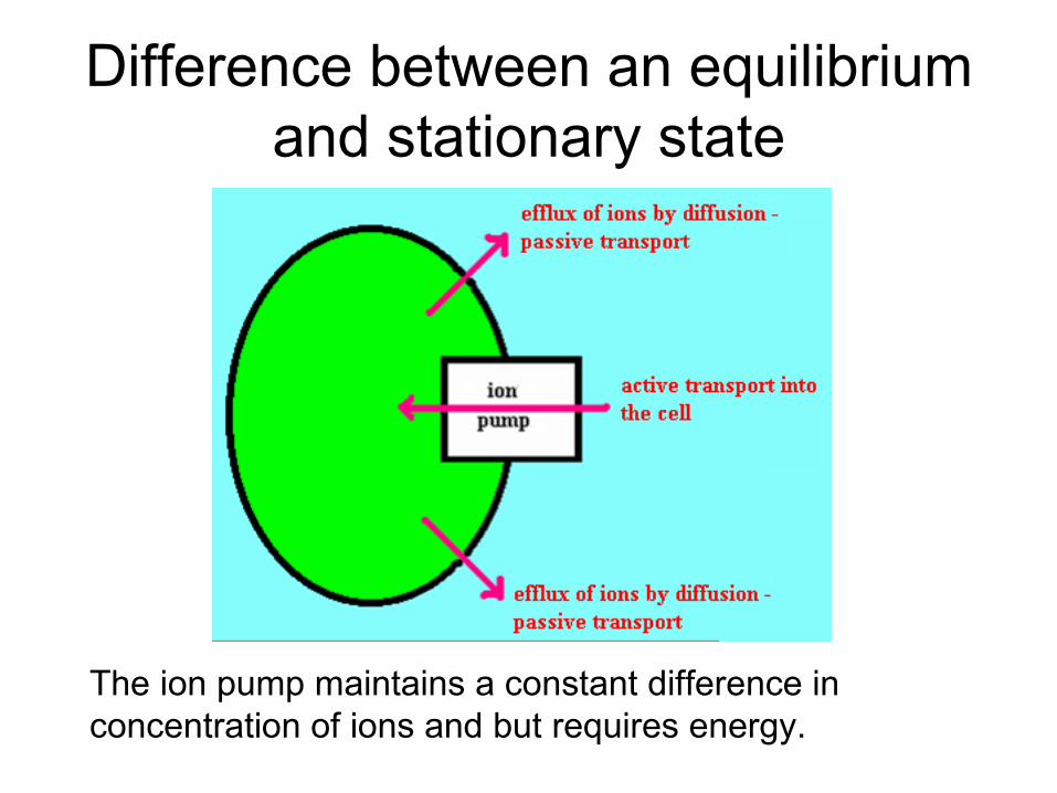
Difference between an equilibrium and stationary state

The temperature difference can be maintained only in an open system involving a heat pump which requires an energy input to function.

Heat pump

Difference between an equilibrium and stationary state

The ion pump maintains a constant difference in concentration of ions and but requires energy.

Fluctuations and generalised le Chatelier principle

• Fluctuations are small deviations from the equilibrium or stationary state arising from internal stochastic (random) processes. Small disturbances are small deviations from the equilibrium or stationary state arising from external processes.

• Generalised le Chatelier principle:– When a system is at a stationary state, any small fluctuations

lead to fluxes of particles or energy which cause the system to return to the original stationary state.

• Critical or bifurcation point (from this point the system can develop in two different ways – e.g. return to the original stationary state or go to another one)

Dissipative structures

• Ordered non-equilibrium time-space structures are called dissipative structures. We cannot apply Boltzmann formula on them. According to Prigogine, they originate as a consequence of a fluctuation. They are stabilised by energy exchange with environment. The dissipative structures belong among problems solved by non-linear non-equilibrium thermodynamics. They can appear only in conditions far enough from equilibrium and a sufficient energy and substance flow is necessary. (Example: „Bénard instability“)

Autocatalytic reactions• A general equation of the autocatalytic reaction:

nA + X ←→ 2X + (n - 1)A, It can be followed by:

X ←→ F• In the autocatalytic reaction, a compound X is formed from

compound A under in presence of the substance X. It means that the substance X acts as a catalyst in its formation. When the substance A is available in sufficient amount, the amount of X grows exponentially. F can be a product formed from compound X.

• Autocatalytic reaction of it's kind is also the replication of DNA. It should be admitted that a complex of „common“ chemical reactions can demonstrate itself as an autocatalytic reaction.

• The replication of DNA is a complex of metabolic processes which results in formation of a copy carrying the same genetic information.

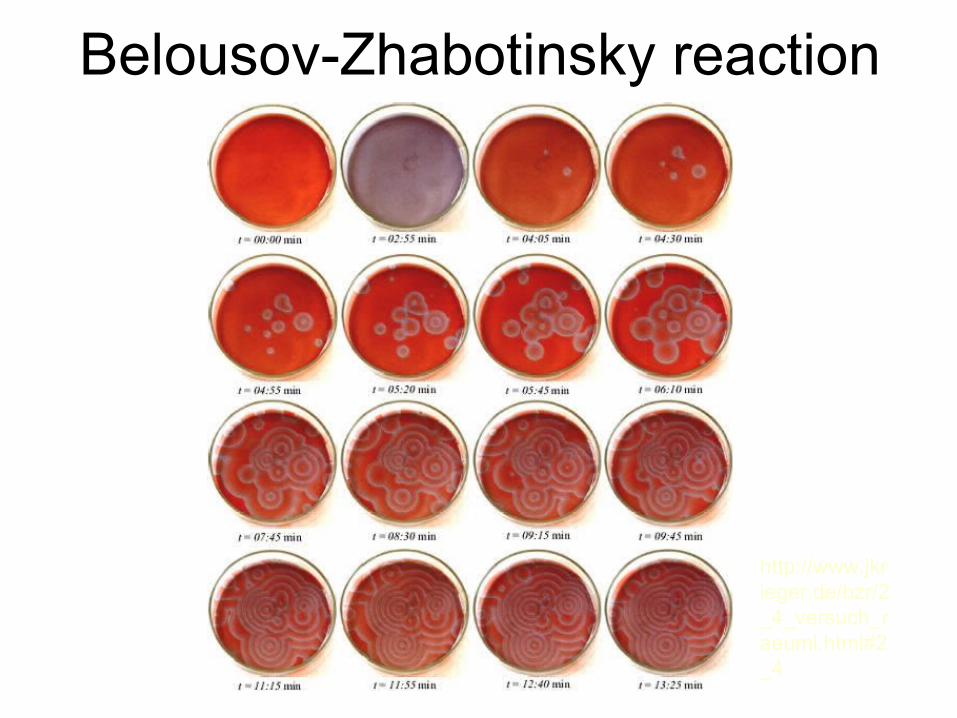
Belousov-Zhabotinsky reaction

http://www.jkrieger.de/bzr/2_4_versuch_raeuml.html#2_4

Examples of thermodynamic approach to problem solution:

Non-equilibrium thermodynamics:

Diffusion

Equilibrium thermodynamics:

Osmosis

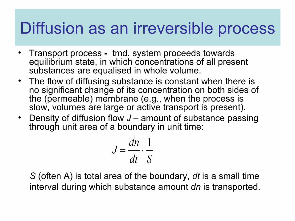
Diffusion as an irreversible process• Transport process - tmd. system proceeds towards

equilibrium state, in which concentrations of all present substances are equalised in whole volume.

• The flow of diffusing substance is constant when there is no significant change of its concentration on both sides of the (permeable) membrane (e.g., when the process is slow, volumes are large or active transport is present).

• Density of diffusion flow J – amount of substance passing through unit area of a boundary in unit time:

S (often A) is total area of the boundary, dt is a small time interval during which substance amount dn is transported.

1st Fick lawA.E. Fick (1885):(substance moves in the direction of the x-axis, one-dimensional case of diffusion):

D - diffusion coefficient [m2.s-1]Typical values of D:from 1.10-9 for small molecules to 1.10-12 for big macromolecules

Concentration gradient

Diffusion coefficient

• Approximate formula for the diffusion coefficient was derived by A. Einstein:

k is Boltzmann constantT is thermodynamic temperatureη is dynamic viscosityr is particle radius.

The term 6π.h.r is called friction or hydrodynamic coefficient f .

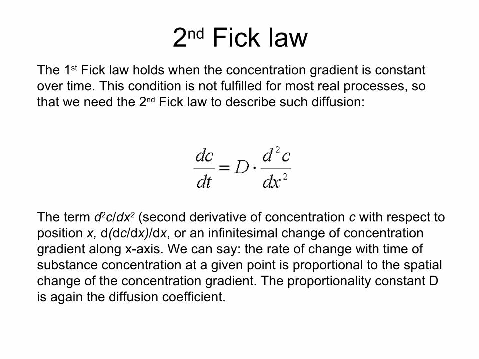
2nd Fick lawThe 1st Fick law holds when the concentration gradient is constant over time. This condition is not fulfilled for most real processes, so that we need the 2nd Fick law to describe such diffusion:

The term d2c/dx2 (second derivative of concentration c with respect to position x, d(dc/dx)/dx, or an infinitesimal change of concentration gradient along x-axis. We can say: the rate of change with time of substance concentration at a given point is proportional to the spatial change of the concentration gradient. The proportionality constant D is again the diffusion coefficient.

Osmosis and osmotic pressure

Solvent can pass through the membrane but not the solute. System proceeds to tmd. equilibrium by equalisation of concentrations of substances in the whole system by solvent diffusion from space I into the space II.

Result: pressure increase in space II.

Pfeffer experiment

van't Hoff formula

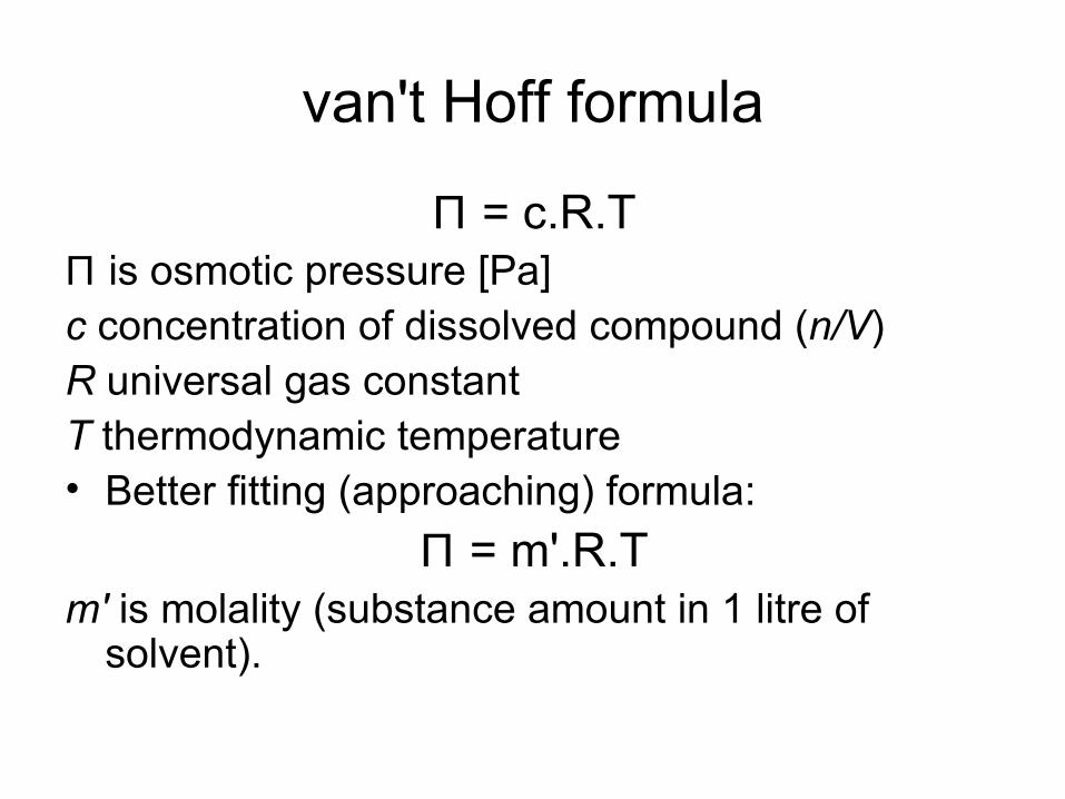
Π = c.R.TΠ is osmotic pressure [Pa]c concentration of dissolved compound (n/V)R universal gas constantT thermodynamic temperature• Better fitting (approaching) formula:

Π = m'.R.Tm' is molality (substance amount in 1 litre of

solvent).

van't Hoff formula

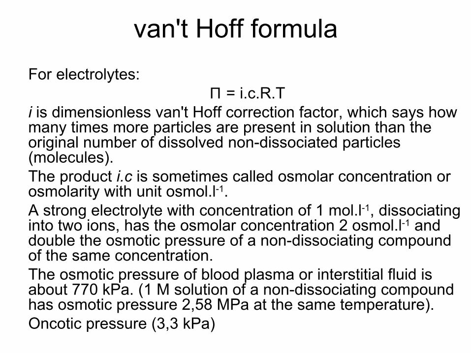
For electrolytes:Π = i.c.R.T

i is dimensionless van't Hoff correction factor, which says how many times more particles are present in solution than the original number of dissolved non-dissociated particles (molecules). The product i.c is sometimes called osmolar concentration or osmolarity with unit osmol.l-1.A strong electrolyte with concentration of 1 mol.l-1, dissociating into two ions, has the osmolar concentration 2 osmol.l-1 and double the osmotic pressure of a non-dissociating compound of the same concentration.The osmotic pressure of blood plasma or interstitial fluid is about 770 kPa. (1 M solution of a non-dissociating compound has osmotic pressure 2,58 MPa at the same temperature).Oncotic pressure (3,3 kPa)

Tonicity of solutions

• solutions having osmotic pressure lower than blood plasma has are hypotonic, with the same pressure are isotonic, and with higher pressure than blood plasma are hypertonic.

• endoosmosis: haemolysis• The range of concentrations of hypotonic

solutions in which partial or full haemolysis does not occur = osmotic resistance of erythrocytes.

• exoosmosis: plasmorrhysis (in plants - plasmolysis)

• receptors (volumoreceptors in kidneys and osmoreceptors in hypothalamus)

How does it look?

Echinocytes – erythrocytes exposed to a hypertonic solution. http://webteach.mccs.uky.edu/COM/pat823/online_materials/diglectures/rbcs/imgshtml/image36.html

Plasmolysis of epidermal cells of onion in hypertonic medium.

http://www.pgjr.alpine.k12.ut.us/science/whitaker/Cell_Chemistry/Plasmolysis.html

Author: Vojtěch Mornstein

Language revision: Carmel J. Caruana

Presentation design: - - -

Last revision: June 2009