thermodynamics lecture series email: [email protected] . [email protected] applied...
TRANSCRIPT

Thermodynamics Lecture Series
email: [email protected]://www5.uitm.edu.my/faculties/f
sg/drjj1.html
Applied Sciences Education Research Group (ASERG)
Faculty of Applied SciencesUniversiti Teknologi MARA
Ideal Rankine Cycle –Ideal Rankine Cycle –The Practical CycleThe Practical Cycle
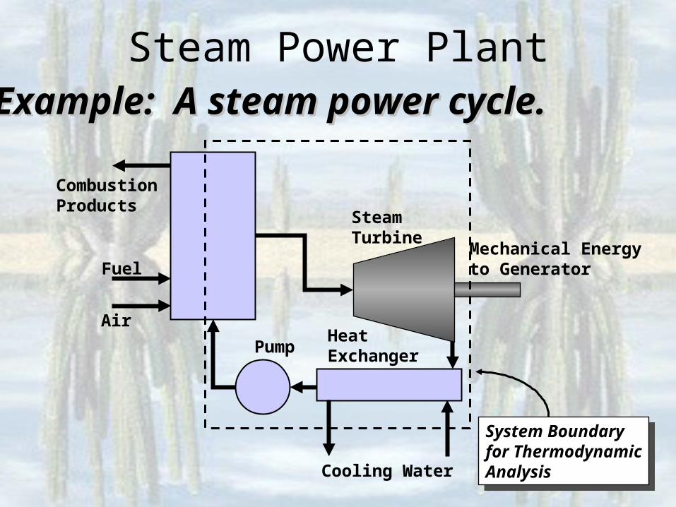
Example: A steam power cycle.Example: A steam power cycle.
SteamTurbine
Mechanical Energyto Generator
Heat Exchanger
Cooling Water
Pump
Fuel
Air
CombustionProducts
System Boundaryfor ThermodynamicAnalysis
System Boundaryfor ThermodynamicAnalysis
Steam Power Plant

Second LawSecond Law
Steam Power Plant
High T Res., TH
Furnace
qin = qH
net,out
Low T Res., TL
Water from river
An Energy-Flow diagram for a SPP
qout = qL
Working fluid:
Water Purpose:
Produce work,
Wout, out
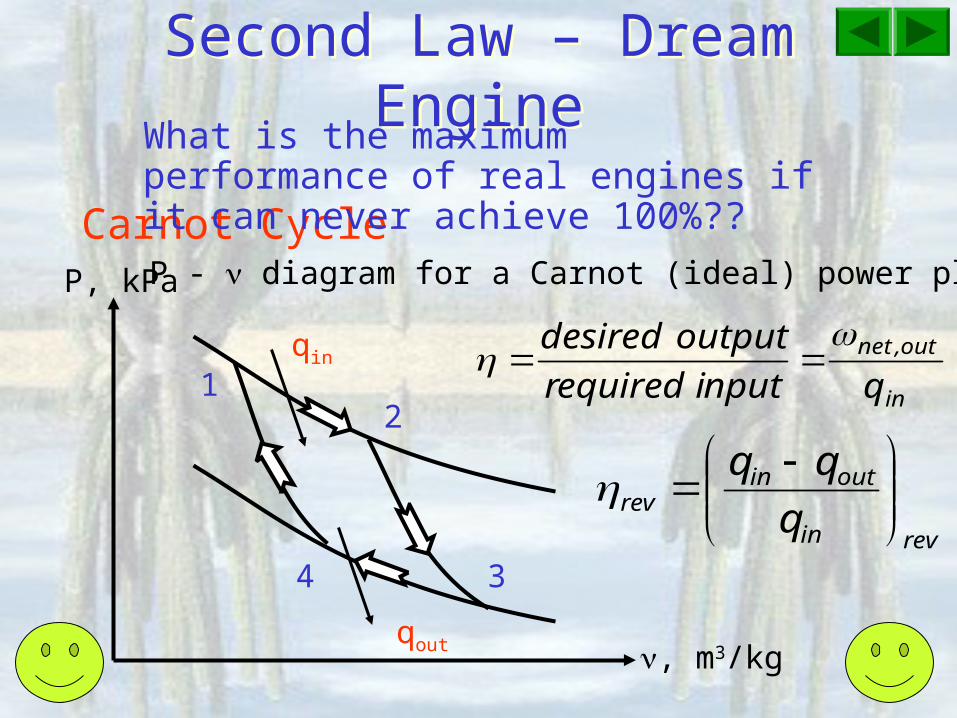
Second Law – Dream EngineSecond Law – Dream Engine
Carnot CycleP - diagram for a Carnot (ideal) power plantP, kPa
, m3/kgqout
qin
2
34
1
What is the maximum performance of real engines if it can never achieve 100%??
in
out,net
qnputi equiredr
output desired
revin
outinrev q

Carnot Principles• For heat engines in contact with the
same hot and cold reservoir P1: 1 = 2 = 3 (Equality)P2: real < rev (Inequality)
Second Law – Will a Process HappenSecond Law – Will a Process Happen
Processes satisfying Carnot Principles obeys the Second Law of
Thermodynamics
revreal
;(K)
(K)
H
L
revH
L
T
T
q
q
(K)
(K) 11
H
L
revH
Lrev T
T
q
q
Consequence

Clausius Inequality :• Sum of Q/T in a cyclic process must be
zero for reversible processes and negative for real processes
K
kJ ,0
T
Q
Second Law – Will a Process HappenSecond Law – Will a Process Happen
,0T
Q
,0T
Q
Kkg
kJ ,0
T
q
reversible
impossible
real
,0T
Q
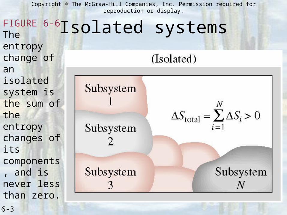
Copyright © The McGraw-Hill Companies, Inc. Permission required for reproduction or display.
6-3
FIGURE 6-6The entropy change of an isolated system is the sum of the entropy changes of its components, and is never less than zero.
Isolated systems
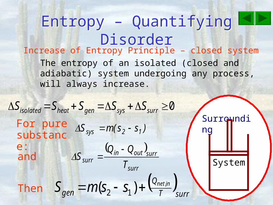
Increase of Entropy Principle – closed systemThe entropy of an isolated (closed and adiabatic) system undergoing any process, will always increase.
Entropy – Quantifying DisorderEntropy – Quantifying Disorder
Surrounding
System
0 surrsysgenheatisolated SSSSS
)ss(mS 12sys
surr
surroutinsurr T
QQS
For pure substance:
surrT
Q
geninnetssmS ,)( 12
and
Then
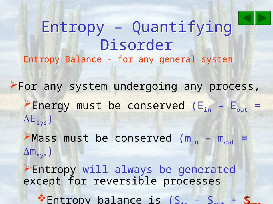
Entropy Balance – for any general system
Entropy – Quantifying DisorderEntropy – Quantifying Disorder
For any system undergoing any process,
Energy must be conserved (Ein – Eout = Esys)
Mass must be conserved (min – mout = msys)
Entropy will always be generated except for reversible processes
Entropy balance is (Sin – Sout + SSgengen = Ssys)

Copyright © The McGraw-Hill Companies, Inc. Permission required for reproduction or display.
6-18
FIGURE 6-61Mechanisms of entropy transfer for a general system.
Entropy Transfer
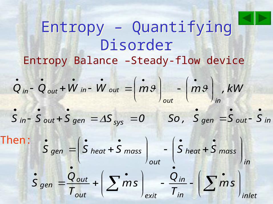
Entropy Balance –Steady-flow device
Entropy – Quantifying DisorderEntropy – Quantifying Disorder
outinoutin WWQQ
kW ,mminout
0SSSS sysgenoutin
inoutgen SSS,So
Then:
in
massheat
out
massheatgen SSSSS
inletin
in
exitout
outgen sm
T
Qsm
T
QS

Entropy Balance –Steady-flow device
Entropy – Quantifying DisorderEntropy – Quantifying Disorder
outinoutin WWQQ
kW ,m inletexit
Turbine:
kW ,000 34 hhmW out
Assume adiabatic, kemass = 0,
pemass = 0
where
mmm exitinlet
K
kWssmS gen ,00 34
EntropyBalance K
kWsmsm
T
Q
T
QS
in
in
out
outgen ,3344
In,3
Out

Entropy Balance –Steady-flow device
Entropy – Quantifying DisorderEntropy – Quantifying Disorder
outinoutin WWQQ
kW ,mminletexit
K
kW,smsmsm
T
Q
T
QS 112233
in
in
out
outgen
Mixing Chamber:
exitinlet mm
where
kW,hmhmhmWWQQ 112233outinoutin
1
3
2
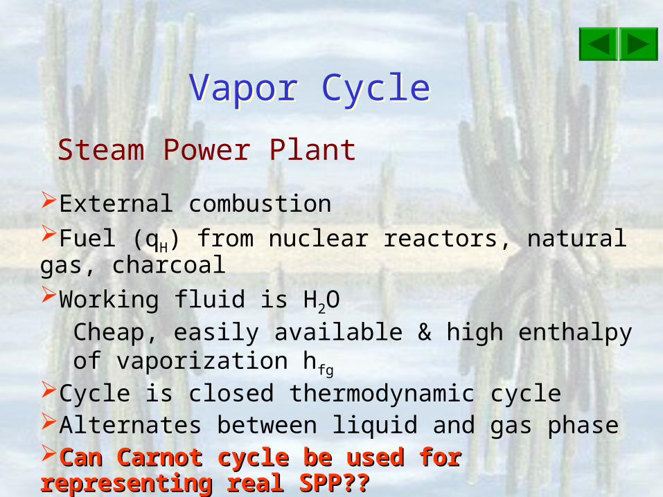
Steam Power Plant
Vapor Cycle Vapor Cycle
External combustionFuel (qH) from nuclear reactors, natural gas, charcoal Working fluid is H2O
Cheap, easily available & high enthalpy of vaporization hfg
Cycle is closed thermodynamic cycleAlternates between liquid and gas phaseCan Carnot cycle be used for representing Can Carnot cycle be used for representing real SPP??real SPP??Aim: To decrease ratio of TL/TH

Efficiency of a Carnot Cycle SPP
Vapor Cycle – Carnot CycleVapor Cycle – Carnot Cycle
55.0273374
273151
T
T1
H
Lrev
627.0273500
273151
T
T1
H
Lrev

Impracticalities of Carnot Cycle
Vapor Cycle –Carnot CycleVapor Cycle –Carnot Cycle
Isothermal expansion: TH
limited to only Tcrit for H2O. High moisture at turbine
exit Not economical to design
pump to work in 2-phase (end of Isothermal compression)
No assurance can get same xfor every cycle (end ofIsothermal compression)s3 = s4s1 = s2
qin = qH
T, C
Tcrit
TH
TL
qout = qL
s, kJ/kgK

Impracticalities of Alternate Carnot Cycle
Vapor Cycle – Alternate Carnot CycleVapor Cycle – Alternate Carnot Cycle
s3 = s4s1 = s2
qin = qHT, C
Tcrit
TH
TL
qout = qL
s, kJ/kgK
Still ProblematicIsothermal expansion but at
variable pressurePump to very high pressure
Can the boiler sustain the high P?
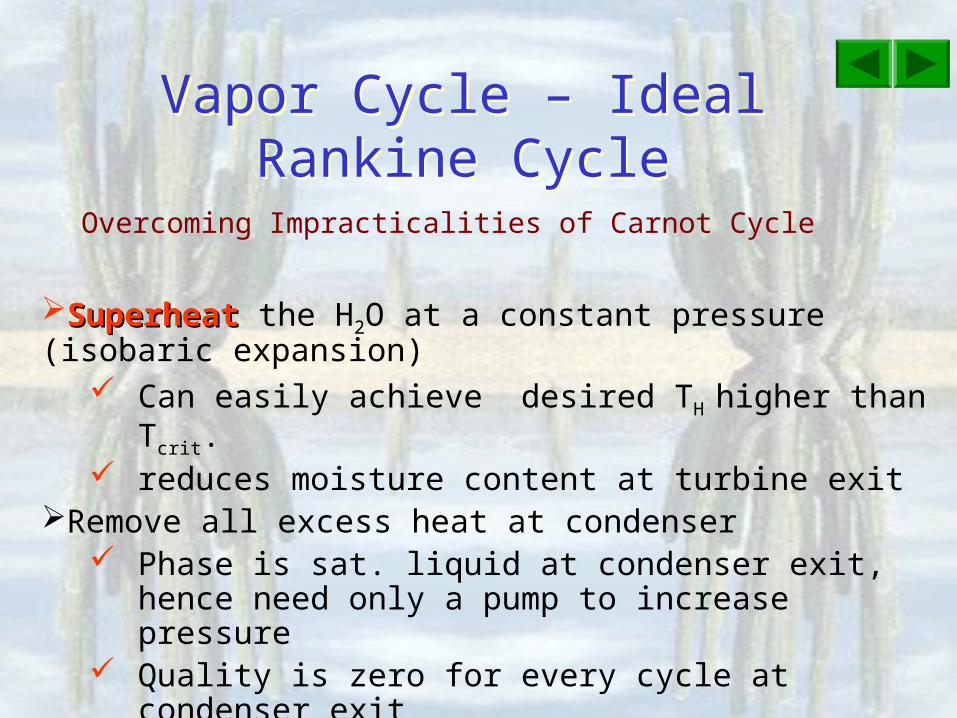
Overcoming Impracticalities of Carnot Cycle
Vapor Cycle – Ideal Rankine CycleVapor Cycle – Ideal Rankine Cycle
SuperheatSuperheat the H2O at a constant pressure (isobaric expansion) Can easily achieve desired TH higher than Tcrit. reduces moisture content at turbine exit
Remove all excess heat at condenser Phase is sat. liquid at condenser exit, hence
need only a pump to increase pressure Quality is zero for every cycle at condenser exit
(pump inlet)

Vapor Cycle – Ideal Rankine CycleVapor Cycle – Ideal Rankine Cycle
Pum
p
Boiler
Turbin
e
Condenser
High T Res., TH
Furnace
qin = qH
inout
Low T Res., TL
Water from river
A Schematic diagram for a Steam Power Plant
qout = qL
Working fluid:
Water
qin - qout = out - in
qin - qout = net,out

T- s diagram for an Ideal Rankine Cycle
Vapor Cycle – Ideal Rankine CycleVapor Cycle – Ideal Rankine Cycle
T, C
s, kJ/kgK
1
2
Tcrit
TH
TL= Tsat@P4
Tsat@P2
s3 = s4s1 = s2
qin = qH
4
3
PH
PL
in
out
pump
qout = qL
condenser
turbineboiler

Copyright © The McGraw-Hill Companies, Inc. Permission required for reproduction or display.
9-2
FIGURE 9-2The simple ideal Rankine cycle.
Vapor Cycle – Ideal Rankine CycleVapor Cycle – Ideal Rankine Cycle
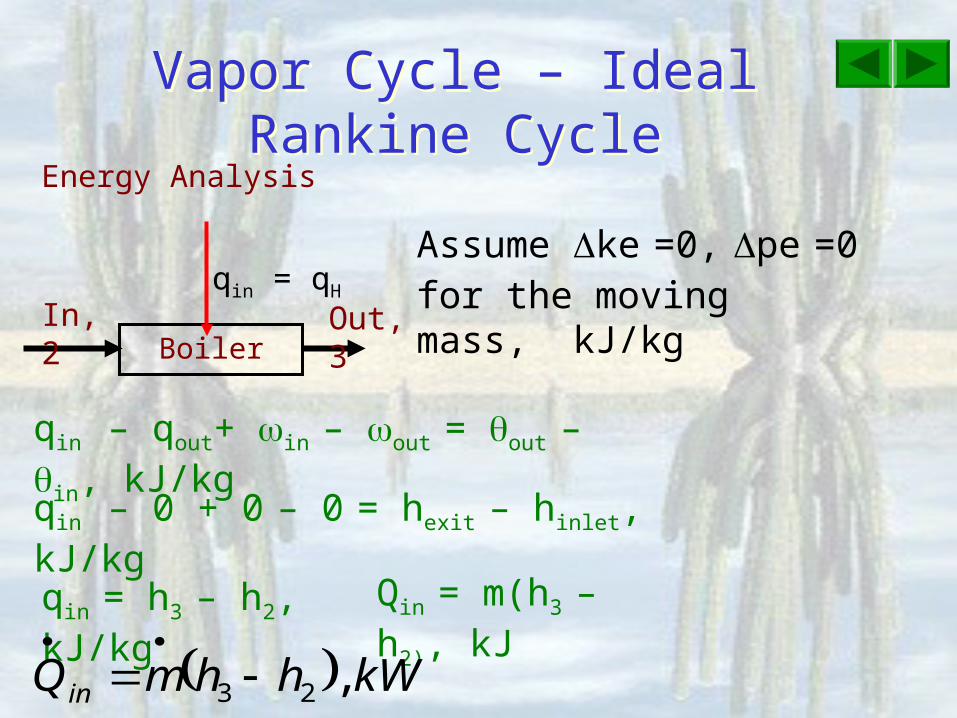
BoilerIn,2 Out,3
qin = qH
Energy Analysis
qin – qout+ in – out = out – in, kJ/kg
qin – 0 + 0 – 0 = hexit – hinlet, kJ/kg
qin = h3 – h2, kJ/kg
Assume ke =0, pe =0 for the moving mass, kJ/kg
Qin = m(h3 – h2), kJ
kWhhmQin ,23
Vapor Cycle – Ideal Rankine CycleVapor Cycle – Ideal Rankine Cycle
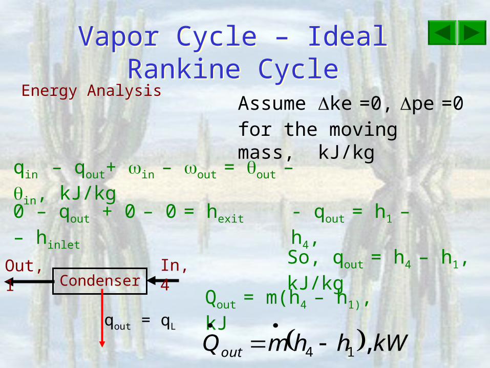
CondenserOut,1 In,4
qout = qL
Energy Analysis
qin – qout+ in – out = out – in, kJ/kg
0 – qout + 0 – 0 = hexit – hinlet - qout = h1 – h4,
So, qout = h4 – h1, kJ/kg
Assume ke =0, pe =0 for the moving mass, kJ/kg
Qout = m(h4 – h1), kJ
kWhhmQout ,14

Vapor Cycle – Ideal Rankine CycleVapor Cycle – Ideal Rankine CycleEnergy Analysis
qin – qout+ in – out = out – in, kJ/kg
0 – 0 + – out = hexit – hinlet, kJ/kg
- out = h4 – h3, kJ/kg So,out = h3 – h4, kJ/kg
out
In,3
Out,4
Turbin
e
Assume ke =0, pe =0 for the moving mass, kJ/kg
Wout = m(h3 – h4), kJ
kWhhmW out ,43

Vapor Cycle – Ideal Rankine CycleVapor Cycle – Ideal Rankine CycleEnergy Analysis
qin – qout+ in – out = out – in, kJ/kg
0 – 0 + in – = hexit – hinlet, kJ/kg
in = h2 – h1, kJ/kg
Pum
pin
Out,2
In,1
2
1
2
1
2
1in,pump dP0dPPd
1212in,pump hhPP
For reversible pumps
where1P@f12
So, Win = m(h2 – h1), kJ
kWhhmW in ,12
Vapor Cycle – Ideal Rankine CycleVapor Cycle – Ideal Rankine CycleEnergy Analysis
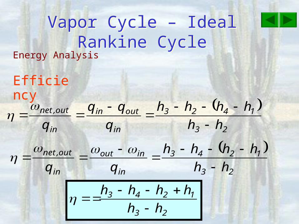
23
1423
in
outin
in
out,net
hh
hhhh
q
q
Efficiency
23
1243
in
inout
in
out,net
hh
hhhh
23
1243
hh
hhhh
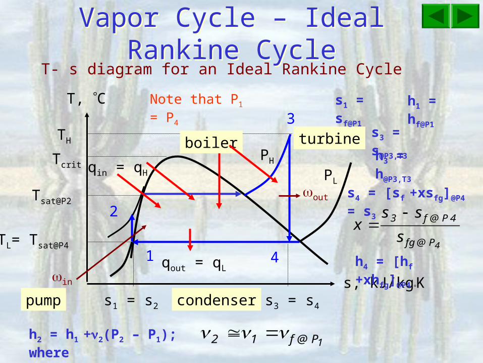
T- s diagram for an Ideal Rankine Cycle
Vapor Cycle – Ideal Rankine CycleVapor Cycle – Ideal Rankine Cycle
T, C
s, kJ/kgK
1
2
Tcrit
TH
TL= Tsat@P4
Tsat@P2
s3 = s4s1 = s2
qin = qH
4
3
PH
PL
in
out
pump
qout = qL
condenser
turbineboiler
s1 = sf@P1 h1 = hf@P1
s3 = s@P3,T3
s4 = [sf +xsfg]@P4 = s3
h3 = h@P3,T3
h4 = [hf +xhfg]@P4
4P@fg
4P@f3
s
ssx
h2 = h1 +2(P2 – P1); where1P@f12
Note that P1 = P4
Vapor Cycle – Ideal Rankine CycleVapor Cycle – Ideal Rankine CycleEnergy Analysis
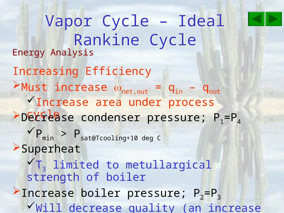
Increasing EfficiencyMust increase net,out = qin – qout
Increase area under process cycleDecrease condenser pressure; P1=P4
Pmin > Psat@Tcooling+10 deg C
Superheat T3 limited to metullargical strength of boiler
Increase boiler pressure; P2=P3
Will decrease quality (an increase in moisture). Minimum x is 89.6%.

Copyright © The McGraw-Hill Companies, Inc. Permission required for reproduction or display.
9-4
FIGURE 9-6The effect of lowering the condenser pressure on the ideal Rankine cycle.
Lowering Condenser Pressure

Copyright © The McGraw-Hill Companies, Inc. Permission required for reproduction or display.
9-5
FIGURE 9-7The effect of superheating the steam to higher temperatures on the ideal Rankine cycle.
Superheating Steam

Copyright © The McGraw-Hill Companies, Inc. Permission required for reproduction or display.
9-6
FIGURE 9-8The effect of increasing the boiler pressure on the ideal Rankine cycle.
Increasing Boiler Pressure

Copyright © The McGraw-Hill Companies, Inc. Permission required for reproduction or display.
9-8
FIGURE 9-10T-s diagrams of the three cycles discussed in Example 9–3.

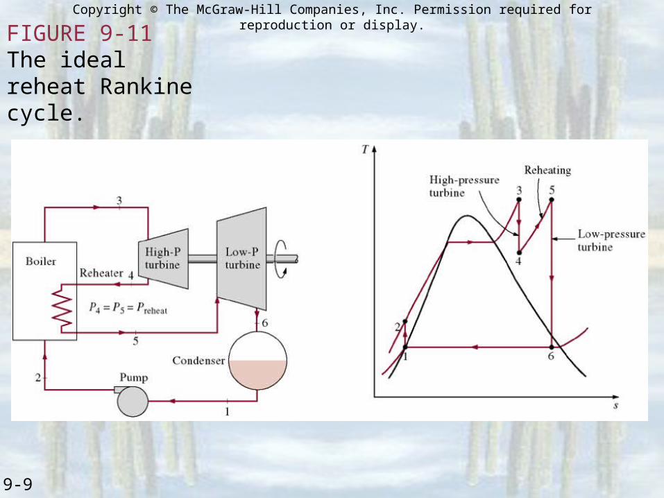
Vapor Cycle – Reheat Rankine CycleVapor Cycle – Reheat Rankine CycleP
ump
Boiler Hig
h P
turbine
Condenser
High T Reservoir, TH
qin = qH
in
out,1
qout = qL
Low T Reservoir, TL
Low P
turbine out,2
1
2
3
4
5
6
qreheat
Copyright © The McGraw-Hill Companies, Inc. Permission required for reproduction or display.
FIGURE 9-11The ideal reheat Rankine cycle.
9-9
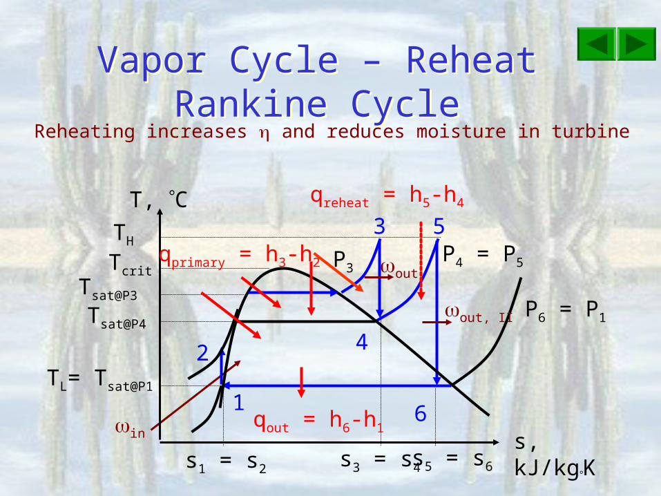
Reheating increases and reduces moisture in turbine
Vapor Cycle – Reheat Rankine CycleVapor Cycle – Reheat Rankine Cycle
TL= Tsat@P1
in
s5 = s6s1 = s2
Tcrit
TH
Tsat@P4
Tsat@P3
s3 = s4
qout = h6-h1
out, II
P4 = P5
P6 = P1
61
5
4
qreheat = h5-h4
qprimary = h3-h2 outP3
3
2
T, C
s, kJ/kgK

Energy Analysis
Vapor Cycle – Reheat Rankine CycleVapor Cycle – Reheat Rankine Cycle
q in = qprimary + qreheat = h3 - h2 + h5 - h4 qout = h6-h1
net,out = out,1 + out,2 - in = h3 - h4 + h5 - h6 – h2 + h1
4523
164523
in
outin
in
out,net
hhhh
hhhhhh
q
q
4523
12654321,
hhhh
hhhhhh
qq in
inoutout
in
outnet
Energy Analysis
Vapor Cycle – Reheat Rankine CycleVapor Cycle – Reheat Rankine Cycle
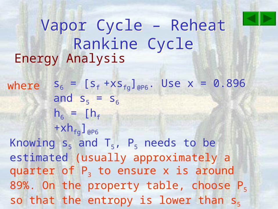
where s6 = [sf +xsfg]@P6. Use x = 0.896 and s5 = s6
Knowing s5 and T5, P5 needs to be estimated (usually approximately a quarter of P3 to ensure x is around 89%. On the property table, choose P5 so that the entropy is lower than s5 above. Then can find h5 = h@P5,T5.
h6 = [hf +xhfg]@P6

Energy Analysis
Vapor Cycle – Reheat Rankine CycleVapor Cycle – Reheat Rankine Cycle
s1 = sf@P1where
s3 = s@P3,T3 = s4.
h1 = hf@P1
h3 = h@P3,T3
h2 = h1 +2(P2 – P1); where1P@f12
From P4 and s4, lookup for h4 in the table. If not found, then do interpolation.
P5 = P4.

Copyright © The McGraw-Hill Companies, Inc. Permission required for reproduction or display.
9-7
FIGURE 9-9A supercritical Rankine cycle.
Supercritical Rankine Cycle