thesis an analysis of the dairy industry: regional impacts
TRANSCRIPT

THESIS
AN ANALYSIS OF THE DAIRY INDUSTRY: REGIONAL IMPACTS AND RATIONAL
PRICE FORMATION
Submitted by
Graham Swanepoel
Department of Agricultural and Resource Economics
In partial fulfillment of the requirements
For the Degree of Master of Science
Colorado State University
Fort Collins, Colorado
Summer 2014
Master’s Committee:
Advisor: Joleen Hadrich
Stephen R. Koontz
Craig McConnel

Copyright by Graham Swanepoel 2014
All Rights Reserved

ii
ABSTRACT
AN ANALYSIS OF THE DAIRY INDUSTRY: REGIONAL IMPACTS AND RATIONAL
PRICE FORMATION
In the first chapter an Input-Output model was used to estimate the economic contribution of
the combined dairy industry to the local Colorado economy. Due to the substantial increase in
the dairy industry over the last decade, there was need to quantify the economic role of dairy
industry, from dairy producers to dairy processers, and measure the linkages with allied
industries in terms of output, value added, and employment contributions. It was estimated that
the total economic contribution of the dairy industry exceeded $3 billion in 2012, and accounted
for roughly 4,333 jobs.
In the chapter two Class III milk futures contracts are examined for the presence of rational
price formation due to increasing uncertainty surrounding revenue streams for dairy producers.
Presence of rational price formation suggests an efficient market, allowing for increased
confidence in the futures market. A system of 12 seemingly unrelated regressions is used to
investigate rational price formation. Futures contracts are found to be acting in an allocative
capacity from 11 months to 3 months prior to expiration month. In the last 2 months, the forward
pricing role is dominant taking into account the supply and demand dynamics in the market. It is
found that Class III milk futures play both roles well, indicating that they are efficient in utilizing
all information available through the last 12 months of trading.

iii
TABLE OF CONTENTS
ABSTRACT .................................................................................................................................................. ii
CHAPTER 1: ECONOMIC CONTRIBUTION OF THE DAIRY INDUSTRY TO THE COLORADO
ECONOMY .................................................................................................................................................. 1
REFERENCES ........................................................................................................................................... 26
CHAPTER 2: BRINGING TRANSPARENCY TO CLASS III MILK FUTURES: EVIDENCE
OF RATIONAL PRICE FORMATION ............................................................................................... 28
REFERENCES ........................................................................................................................................... 56

1
Chapter One:
Economic Contribution of the Dairy Industry to the Colorado Economy
Introduction
The Pacific and Mountain dairy states1 have significantly increased their share of the United
States (US) national dairy herd and now account for approximately 38% of the total dairy cows
in the US (USDA, 2012). Pacific and Mountain dairy states have increased herd size by 14% and
29% correspondingly from 2000 to 2012, while more traditional dairy regions such as the
Northeast and Lake2 States have decreased 18% and 3%, respectively. This information implies
a pattern of transfer of production out of the traditional dairy regions to the Pacific and Mountain
regions.
Within the Mountain dairy region, Colorado has experienced some of the highest growth.
Colorado is seen as a promising dairy location due the space available, proximity to feed inputs,
and expected population growth in the state (Pritchett, Thorvaldson, & Fraiser, 2006). Table 1.1
shows the evolution of the Colorado dairy industry from 2000 to 2012; cow numbers have
increased 51% to 134,000, and total production by 67% to 3.2 million pounds of milk over the
same time period (USDA, 2012). As the role of dairy farms have increased in states regarded as
relatively new dairy producing states, quantifying the economic contribution of the industry
becomes necessary (Cabrera et. al, 2008).
1 USDA Region Classification: Pacific Region: Washington, Oregon, California, Alaska, and Hawaii.
Mountain Region: Montana, Nevada, Arizona, New Mexico, Colorado, Utah, Wyoming, and Idaho. USDA (2012) 2 USDA Region Classification: Northeast: Maine, New Hampshire, Vermont, Massachusetts, Rhode Island,
Connecticut, New York, New Jersey, Pennsylvania, Delaware, Maryland. Lake States: Michigan, Wisconsin,
Minnesota. USDA (2012)

2
Table 1.1. Colorado Dairy Industry Growth
2000 2012 % Increase
Cow numbers (thousands) 89 134 51%
Milk per cow (lbs/yr) 21,618 23,978 11%
Total milk prod (mil. lbs) 1,924 3,213 67%
Three reasons have been identified for quantifying the economic contribution of the dairy
industry to a state; use in policy decisions, benefits for society, and potential effect on linked
industries (Cabrera et. al, 2008). Helmburger & Chen (1994) examined the short and long term
benefits and costs of terminating milk support programs. Through an analysis of three policy
options, they were able to identify the contribution of dairy farms to the economy under each
scenarios. Balagtas et al. (2003) studied potential repercussions for linked industries and the
overall benefits to society. Through an investigation of new markets and uses for current
agricultural products, they were able to anticipate the effect on the market of innovations. In
addition to the three primary reasons to quantify the economic contribution of the dairy industry,
it also provides a sense of pride for dairy farmers in the state, and provides the public with an
awareness of the economic contribution the dairy farm industry to the community (Cabrera et. al,
2008). Day and Minnesota IMPLAN Group Inc. (2013) list other uses of impact or contribution
analysis, ranging from effective ways to invest into local economies, to identifying impacts on
tax revenues.
Economic contribution is defined as the gross change in economic activity associated with an
industry, event, or policy in an existing regional economy. This is not to be confused with impact
analysis, which considers the increase or reduction in total economic activity in a region due to
some event like a new environmental regulation, a change in tax policy, or entrance of a new
business (Watson et al. 2007). Economic contribution analysis generates results broken into

3
three categories; direct, indirect, and induced contributions. Direct economic contributions are
essentially those resulting from the dairy industries purchases, i.e. purchase of feed grain by a
dairy producer, and the jobs which are created in the dairy producer’s operation. Indirect
economic contributions are the revenues from the sale of dairy products re-spent in the local
economy. The indirect contribution of the dairy industry on local economies includes purchases
of a variety of agricultural inputs and professional services by industries supporting the dairy
industry, i.e. a feed supplier has increased purchases of feed to meet the increased demand from
the dairy producer (Day & Minnesota IMPLAN Group Inc., 2013). Indirect contributions can
also appear as jobs and income in local industries serving the dairy industry (vets, feed suppliers,
implement suppliers, trucking and transport). Induced economic contributions are the local goods
and services purchased by people using the salaries and wages earned contributing to the
productivity of the dairy industry (typically thought of as longer term contributions, Cabrera et
al. 2008). The induced effects can be thought of in terms of jobs and income for retailers, bank
tellers, grocery store clerks, restaurant employees, and gas station attendants, among others
(Neibergs & Brady, 2013).
An economic contribution study is a variation of an Input-Output (I-O) model, which should
not be confused with the annual sales of an industry. An I-O model, or economic contribution
study, helps track the flow of money from one entity to another, allowing for the representation
of the interconnectedness of industries, households, and government entities within the study
area (Day & Minnesota IMPLAN Group Inc., 2013), and the sales of an industry is just the
beginning of the analysis. This rationale is important for this study, as the output of one industry
becomes the input for another industry. In the scope of this study, the output from dairy

4
producers becomes the input for the fluid milk and butter processing, as well as the cheese
processing industry. Using sales as a starting point also becomes important in the evaluation of
any shocks to an industry, as the increase or decrease in sales is first step in generating any
potential shocks (Day & Minnesota IMPLAN Group Inc., 2013).
The dairy industry, as part of the broader agricultural sector, is classified as a basic industry
to the Colorado state economy. Basic industries provide income to a region by producing an
output, purchasing production inputs, services and labor. The production of dairy milk and
processing products represent the direct economic contribution of the industry to the locality
(Seidl & Weiler, 2000). This logic dictates the method of further analysis contained within this
paper. We estimate the economic contribution of each of the separate areas contained in the
whole dairy industry; dairy producers, fluid milk and butter manufacturing, cheese
manufacturing, and ice cream and frozen dessert manufacturing. In addition to this, we aggregate
all of previously mentioned areas into a combined industry, which represents the contribution of
the dairy industry as a whole to Colorado.
There is relatively little prior literature that have used I-O analysis to estimate the
contribution of the dairy industry to the state, regional, or local economy. Relevant studies
include Neibergs and Brady (2013), Washington State; Cabrera et al. (2008), New Mexico;
Janssen et al. (2006), alternative sized dairy farms in South Dakota; Hussain et al. (2003), Earth
County, Texas; and Seidl and Weiler, (2000), North Eastern Colorado. Neibergs and Brady
(2013), used a survey of producers to generate primary data used to compare to the I-O generated
results. Seidl and Weiler’s study in 2000 provides us with a unique “starting value”, from which

5
to compare how the economic contribution of the dairy industry has grown over the 12 years
spanning the two studies. I-O analysis has been used extensively in other sectors of the economy.
Within the broader agricultural sector I-O analysis has been used to evaluate the economic
contributions of different sectors to the state or regional economies. Mon and Hooland (2005)
used I-O models to evaluate organic apple production in Washington State, while Daniel,
English, & Jensen, (2007) investigated the effect of increasing ethanol and biofuel production in
the US. Outside of agriculture, I-O models and IMPLAN have been widely used in the forestry
industry. IMPLAN was originally developed by the US Forest Service (Hotvedt, Busby, &
Jacob, 1988) and has continued to be used in studies since, such as Hjerpe, and Kim, (2008) who
analyzed the economic impacts of reducing wildfire risk through various management methods.
In Colorado, the primary use of I-O models have been within the water sector. Gunter et al.
(2012), and McKean and Spencer (2003) both used I-O models in examinations of how to deal
with drought issues in specific watersheds. Howe and Goemans, (2003), and Pritchett,
Thorvaldson, and Fraiser (2006) examined water transfer issues using the I-O methodology, and
Houk, Fraiser and Schuck (2004) used it to study the effects of water logging and soil
salinization. In addition to the areas already mentioned, I-O models have also been used in
regional economic studies (Weiler et al. 2003). The significant body of literature that uses I-O
modeling techniques is a testament to the accuracy and effectiveness of the method, and so was
chosen as the primary method of analysis in the examination of the contribution that dairy has on
the Colorado economy.

6
This paper adds to the limited body of literature on the contribution of the dairy producers
industry to regional economies, and also goes further by quantifying the estimated contribution
of the entire dairy industry to the regional economy. Quantifying the dairy industry provides a
snapshot of the contributions being made to the regional economy, aiding in future economic
analysis, policy making and allowing for the examination of benefits provided to society from
the dairy industry. The work done in this study provides a holistic view of the dairy industry by
examining each sector of the industry, (dairy producers, fluid milk and butter manufacturers,
cheese manufactures, and ice cream and frozen dessert manufacturers), and the industry as a
whole to accurately quantify the contributions made to the local Colorado economy.
The remainder of this paper is organized as follows. The methods and materials section
describes the I-O model in more detail applying it specifically to the Colorado dairy industry
with further descriptions of the data used. The results and conclusion section follows.
Methods and Materials
An I-O analysis was conducted using the IMpact analysis for PLANning (IMPLAN) model
software. First developed by Leontief (1936), the I-O model provides a simple method to
describe an economy by tracing a change in inputs purchased resulting from a shock in final
demand3. I-O models provide estimates of the change in in economic activity, i.e. a change in
total revenues, across all sectors of a local economy resulting from a change in final demand. I-O
analysis uses an economic framework that traces the flow of goods and services, income, and
employment among related sectors in a defined regional economy. Therefore, the results can be
interpreted as a snapshot of a regional economy in equilibrium (Cabrera, et. al, 2008). Linear
3 Final demand is defined as the value of goods and services produced and sold to final users (Minnesota
IMPLAN Group Inc., 2013). This does not include the sale of intermediate goods used as an input to production in
another industry.
7
relationships are used within I-O analysis to reflect production processes that equate industry
inputs and outputs (e.g. dairy farms) within a specific geographic region (e.g., CO). I-O models
are “demand driven” models, in which the demand for the output of an industry can be examined
to determine its impacts on the other sectors of the economy as a result of their interdependences.
The IMPLAN model, as an interpretation of the I-O theory, is based on the US national
income, product accounts, and various other regional data sources. County level data contained
within IMPLAN’s software was used to create the regional economy, which the authors
described as the whole state of Colorado. I-O models are relatively easy to use and results can
be obtained quickly and at a low cost (with the availability of data and software packages, such
as IMPLAN). This model is very widely used so results are comparable to other studies, and all
sectors of a regional economy are included. IMPLAN collect data from the U.S. Bureau of Labor
Statistics (BLS) Covered Employment and Wages (CEW) program, U.S. Bureau of Economic
Analysis (BEA) Regional Economic Information System (Rea) program, and various other4
economic reports (Day & Minnesota IMPLAN Group Inc., 2013).
IMPLAN is a backward economic linkage model, and as such, it only includes the impacts of
the industry being studied. This is one of the main shortcomings of I-O models in that they do
not model impacts to industries in the supply chain that use the output from the primarily
impacted industries (Gunter et al. 2012). For this study, both the dairy producing and processing
sectors are of relevance, so the sum of both economic contributions would be equal to the
importance of the whole dairy industry to Colorado. Stevens et al. (2005) found milk to be
4 U.S. Bureau of Economic Analysis Benchmark I/O Accounts of the U.S., BEA Output estimates, BLS
Consumer Expenditure Survey, U.S. Census Bureau County Business Patterns (CBP) program), U.S. Census Bureau
Decennial Census and Population Surveys, U.S. Census Bureau Economic Censuses and Surveys, U.S. Department
of Agriculture Census. There is a 5 month lag in the data being released to the public due to the collection time (Day
& Minnesota IMPLAN Group Inc., 2013).
8
essentially a necessity with nearly inelastic demand and therefore we have assumed that if there
were no dairy industry in Colorado, then consumers would still buy the same amount of dairy
products, however, these would be imported from outside the region. Dollars spent on imports
would represent a loss to the region (Neibergs & Brady, 2013).
Results of an economic contribution study are usually described in terms of multipliers,
where a multiplier refers to the total amount of economic activity generated by a dollar of export
sales (Seidl & Weiler, 2000). The most common multipliers are Type I (direct + indirect
effects), and Type II or social accounting matrix, SAM (SAM = direct + indirect + induced
effects). These contributions are analyzed in terms of industry outputs, employment, labor
income, and value added to the economy (Day and Minnesota IMPLAN Group Inc., 2013). In
addition to the results of IMPLAN in multiplier form, results are also displayed in dollar terms
for output and value added, and number of employees. For these results, output is described in
terms of dollars of sales per dollar of sales outside the region, and employment is the number of
jobs created per one million dollars of sales (Seidl & Weiler, 2000). Value added is the dollars of
local earnings per dollar of export sales; it can also be described as the difference between an
industry’s total output and the cost of its intermediate inputs. Value added consists of
compensation of employees, taxes on production and imports less subsidies, and gross operating
surplus (Minnesota IMPLAN Group Inc., 2013).
Results and Discussion
Our IMPLAN analysis looks at the dairy industry in its separate entities and then as a whole,
in which the parts are combined into one “dairy industry”. The specific areas of focus were: (1)

9
dairy producers, (2) fluid milk and butter processors, (3) cheese manufacturers, and (4) ice cream
and frozen dessert manufacturing. For each of separate industries we identified multipliers and
the economic contribution towards the Colorado economy. Our last industry is (5) the total
Colorado dairy industry. This industry was generated using the IMPLAN software, and is an
aggregation of all the specific dairy areas mentioned above.
Dairy Producer Sector
The dairy producer industry within Colorado is comprised of dairy cattle and milk producers,
NAICS5 classification 12, and was estimated to have total direct sales of $368,328,484 which
provided $593,525,940 of total economic contribution. Table 1.2 indicates that the dairy
producer industry indirectly contributed $167,155,589 of output to the local economy, as well as
an induced contribution of $58,041,867. There was a $279,439,104 contribution through value
added processes within the industry in the 2012 calendar year. The dairy industry was directly
responsible for a total of 1,238 jobs in the state, while indirect (i.e. suppliers) and induced (i.e.
banks, and groceries) industries contribute 631, and 402 jobs respectively.
The total output multiplier for the dairy producers industry was estimated at 1.61, indicating
that $1.61 total sales take place in Colorado for each dollar of sales outside of Colorado, for
example sales of $1 million of milk generated $1.61 million in local economic activity. Dairy
producers provided an estimated 7 jobs per million dollars of sales, 3.83 directly within the dairy
producers industry, 1.95 indirectly, and 1.24 through induced industries. As a stand-alone
industry, the dairy producer industry ranked as the 130th largest industry in the Colorado
economy.
5 North American Industry Classification System

10
Table 1.2. Dairy Producers- Multipliers and Economic Contribution
Output Value Added Employment Employee Compensation
Direct 1.00 0.47 3.83 0.10
Indirect 0.45 0.16 1.95 0.09
Induced 0.16 0.10 1.24 0.06
Total 1.61 0.73 7.02 0.25
Direct $ 368,328,484 $ 179,867,492 1,238 $ 10,072,020
Indirect $ 167,155,589 $ 61,431,114 631 $ 9,352,637
Induced $ 58,041,867 $ 38,140,498 402 $ 5,728,336
Total $ 593,525,940 $ 279,439,104 2,270 $ 25,152,992
Fluid Milk and Butter Processors
Table 1.3 details the estimates of multipliers and the respective economic contribution from
the fluid milk and butter manufacturing sector in Colorado, NAICS 55. IMPLAN estimated that
direct sales of milk and butter provide $759,565,524 in economic contribution, and resulted in
over $1.6 billion in total economic output for the region in 2012. There was an indirect economic
contribution from the fluid milk and butter sector of over $660 million (i.e. increased sales for
suppliers of inputs to the fluid milk and butter processors) and in excess of $176 million of
induced economic activity (i.e. contribution from industries where labor spend their wages, such
as grocery stores). Value added from fluid milk and butter manufacturing sector provided an
additional $363,482,912 in economic activity.
The sector was estimated to employ a total of 1,140 people statewide, comprised of 134
directly employed in the fluid milk and butter manufacturing, 663 indirectly employed, and a
further 343 people employed in induced industries. An estimated 6.07 jobs will be created for
every $1 million dollars of sales, of which the majority of jobs would occur in indirectly related
industries, such as suppliers to the fluid milk and butter manufacturing industry. A total output
multiplier of 2.11 indicated that $2.11 of total sales take place for every dollar of sales outside

11
Colorado. The fluid milk and butter manufacturing industry, on its own, ranked as the 72nd
largest industry in the Colorado economy.
Table 1.3. Fluid Milk and Butter Manufactures- Multipliers and Economic Contribution
Output Value Added Employment Employee Compensation
Direct 1.00 0.23 0.71 0.09
Indirect 0.88 0.40 3.53 0.20
Induced 0.23 0.15 1.82 0.08
Total 2.11 0.77 6.07 0.37
Direct $ 759,465,524 $ 106,542,389 134 $ 31,882,610
Indirect $ 666,183,459 $ 187,972,635 663 $ 70,904,518
Induced $ 176,049,260 $ 68,967,888 343 $ 30,534,391
Total $ 1,601,698,242 $ 363,482,912 1,140 $ 133,321,518
Cheese Manufacturing
Table 1.4 displays the economic contribution of the cheese manufacturing industry (NAICS
56). A total output of $766,760,610 was derived from direct sales of $368,261,484 in 2012.
Within the output estimates, the cheese industry contributed $325,747,566 through indirect
economic contribution and a further $72,741,560 through induced industries.
The cheese manufacturing industry contributed over $70 million through value added
processes. An output multiplier of 2.08 for the industry indicated $2.08 of local sales for every
$1 dollar of sales of cheese products. The industry was estimated to employ 773 people, 131
within the direct cheese manufacturing, 441 indirectly (i.e. suppliers of inputs needed in the
cheese manufacturing process), and 201 through induced industries (i.e. grocery stores). The
breakdown of jobs shows similarities to that of the fluid milk and butter manufacturing industry,
as most likely the supplier companies are the same. Total employee compensation was estimated
at just over $42 million. IMPLAN analysis estimated that there are almost 6 jobs created for
every $1 million of sales, most of the additional jobs occurred in indirect industries. The cheese
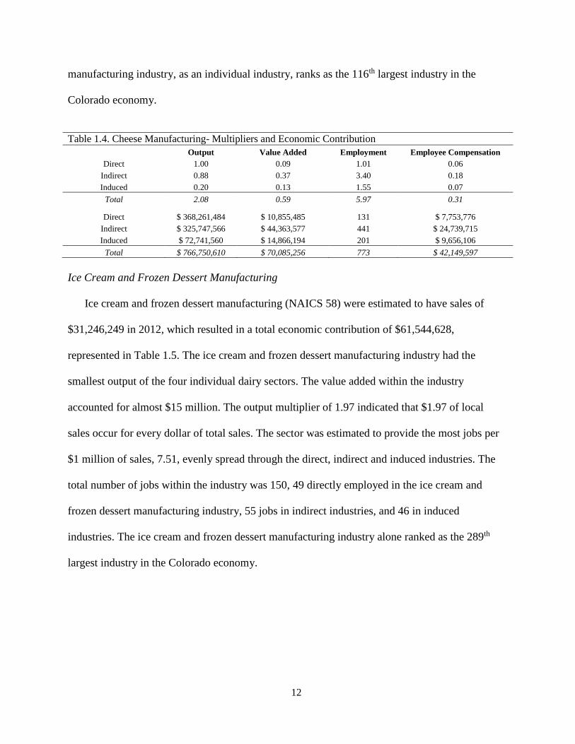
12
manufacturing industry, as an individual industry, ranks as the 116th largest industry in the
Colorado economy.
Table 1.4. Cheese Manufacturing- Multipliers and Economic Contribution
Output Value Added Employment Employee Compensation
Direct 1.00 0.09 1.01 0.06
Indirect 0.88 0.37 3.40 0.18
Induced 0.20 0.13 1.55 0.07
Total 2.08 0.59 5.97 0.31
Direct $ 368,261,484 $ 10,855,485 131 $ 7,753,776
Indirect $ 325,747,566 $ 44,363,577 441 $ 24,739,715
Induced $ 72,741,560 $ 14,866,194 201 $ 9,656,106
Total $ 766,750,610 $ 70,085,256 773 $ 42,149,597
Ice Cream and Frozen Dessert Manufacturing
Ice cream and frozen dessert manufacturing (NAICS 58) were estimated to have sales of
$31,246,249 in 2012, which resulted in a total economic contribution of $61,544,628,
represented in Table 1.5. The ice cream and frozen dessert manufacturing industry had the
smallest output of the four individual dairy sectors. The value added within the industry
accounted for almost $15 million. The output multiplier of 1.97 indicated that $1.97 of local
sales occur for every dollar of total sales. The sector was estimated to provide the most jobs per
$1 million of sales, 7.51, evenly spread through the direct, indirect and induced industries. The
total number of jobs within the industry was 150, 49 directly employed in the ice cream and
frozen dessert manufacturing industry, 55 jobs in indirect industries, and 46 in induced
industries. The ice cream and frozen dessert manufacturing industry alone ranked as the 289th
largest industry in the Colorado economy.
13
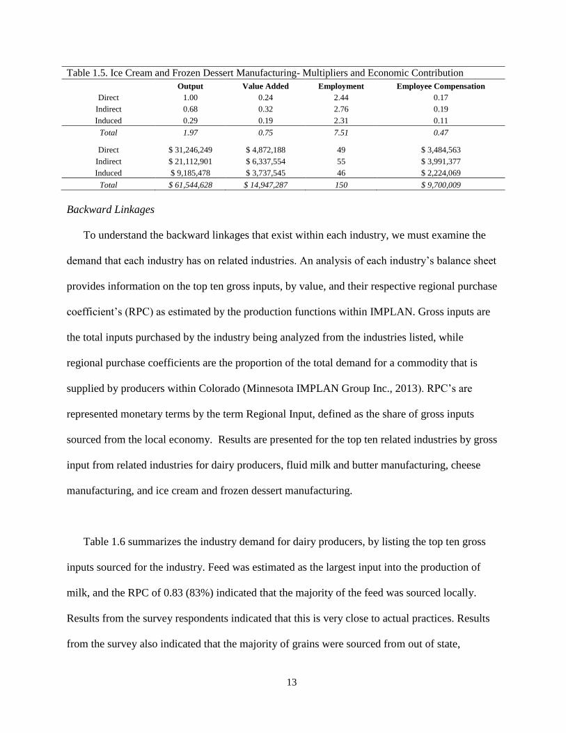
Table 1.5. Ice Cream and Frozen Dessert Manufacturing- Multipliers and Economic Contribution
Output Value Added Employment Employee Compensation
Direct 1.00 0.24 2.44 0.17
Indirect 0.68 0.32 2.76 0.19
Induced 0.29 0.19 2.31 0.11
Total 1.97 0.75 7.51 0.47
Direct $ 31,246,249 $ 4,872,188 49 $ 3,484,563
Indirect $ 21,112,901 $ 6,337,554 55 $ 3,991,377
Induced $ 9,185,478 $ 3,737,545 46 $ 2,224,069
Total $ 61,544,628 $ 14,947,287 150 $ 9,700,009
Backward Linkages
To understand the backward linkages that exist within each industry, we must examine the
demand that each industry has on related industries. An analysis of each industry’s balance sheet
provides information on the top ten gross inputs, by value, and their respective regional purchase
coefficient’s (RPC) as estimated by the production functions within IMPLAN. Gross inputs are
the total inputs purchased by the industry being analyzed from the industries listed, while
regional purchase coefficients are the proportion of the total demand for a commodity that is
supplied by producers within Colorado (Minnesota IMPLAN Group Inc., 2013). RPC’s are
represented monetary terms by the term Regional Input, defined as the share of gross inputs
sourced from the local economy. Results are presented for the top ten related industries by gross
input from related industries for dairy producers, fluid milk and butter manufacturing, cheese
manufacturing, and ice cream and frozen dessert manufacturing.
Table 1.6 summarizes the industry demand for dairy producers, by listing the top ten gross
inputs sourced for the industry. Feed was estimated as the largest input into the production of
milk, and the RPC of 0.83 (83%) indicated that the majority of the feed was sourced locally.
Results from the survey respondents indicated that this is very close to actual practices. Results
from the survey also indicated that the majority of grains were sourced from out of state,
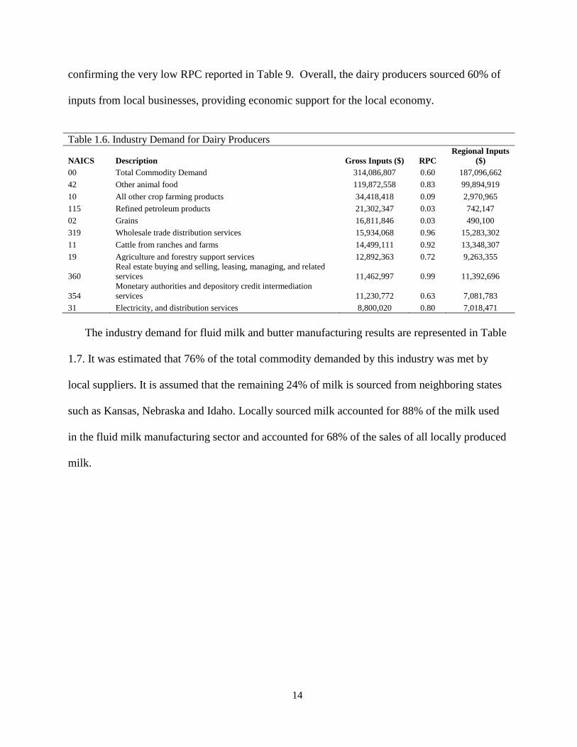
14
confirming the very low RPC reported in Table 9. Overall, the dairy producers sourced 60% of
inputs from local businesses, providing economic support for the local economy.
Table 1.6. Industry Demand for Dairy Producers
NAICS Description Gross Inputs ($) RPC
Regional Inputs
($)
00 Total Commodity Demand 314,086,807 0.60 187,096,662
42 Other animal food 119,872,558 0.83 99,894,919
10 All other crop farming products 34,418,418 0.09 2,970,965
115 Refined petroleum products 21,302,347 0.03 742,147
02 Grains 16,811,846 0.03 490,100
319 Wholesale trade distribution services 15,934,068 0.96 15,283,302
11 Cattle from ranches and farms 14,499,111 0.92 13,348,307
19 Agriculture and forestry support services 12,892,363 0.72 9,263,355
360
Real estate buying and selling, leasing, managing, and related
services 11,462,997 0.99 11,392,696
354
Monetary authorities and depository credit intermediation
services 11,230,772 0.63 7,081,783
31 Electricity, and distribution services 8,800,020 0.80 7,018,471
The industry demand for fluid milk and butter manufacturing results are represented in Table
1.7. It was estimated that 76% of the total commodity demanded by this industry was met by
local suppliers. It is assumed that the remaining 24% of milk is sourced from neighboring states
such as Kansas, Nebraska and Idaho. Locally sourced milk accounted for 88% of the milk used
in the fluid milk manufacturing sector and accounted for 68% of the sales of all locally produced
milk.

15
Table 1.7. Industry Demand for Fluid Milk and Butter Manufacturing
NAICS Description
Gross Inputs
($) RPC
Regional Inputs
($)
00 Total Commodity Demand 1,238,215,340 0.76 938,029,175
12 Dairy cattle and milk products 434,912,820 0.88 381,244,554
55 Fluid milk and butter 220,162,963 0.93 204,652,859
319 Wholesale trade distribution services 62,123,794 0.96 59,586,586
381 Management of companies and enterprises 49,088,152 0.99 48,645,241
335 Truck transportation services 46,378,562 0.80 37,187,976
127 Plastics materials and resins 44,585,435 0.03 1,353,382
107 Paperboard containers 34,604,464 0.48 16,476,510
149 Other plastics products 23,846,824 0.19 4,511,229
57 Dry, condensed, and evaporated dairy products 23,742,482 0.37 8,832,445
31 Electricity, and distribution services 23,289,704 0.80 18,574,741
Table 1.8 summarizes the industry demand for the cheese industry. Of a total of almost $700
million in inputs, Colorado’s local economy provided 64%. Cheese manufacturing sourced 88%
of milk inputs from local producers, but cheese only accounted for 31% of total Colorado milk
sales. As expected, the top ten gross inputs for fluid milk and butter manufacturing, closely
resemble the top ten gross inputs for cheese manufacturing.
Table 1.8. Industry Demand Cheese Manufacturing
NAICS Description Gross Inputs ($) RPC
Regional Inputs
($)
00 Total Commodity Demand 696,665,344 0.64 443,397,977
56 Cheese 242,970,488 0.39 94,807,367
12 Dairy cattle and milk products 200,638,966 0.88 175,880,107
319 Wholesale trade distribution services 46,931,584 0.96 45,014,844
55 Fluid milk and butter 28,839,849 0.93 26,808,131
335 Truck transportation services 22,907,420 0.80 18,367,982
57 Dry, condensed, and evaporated dairy products 20,915,784 0.37 7,780,885
381 Management of companies and enterprises 15,438,227 0.99 15,298,931
142
Plastics packaging materials and un-laminated films and
sheets 8,985,203 0.13 1,126,630
31 Electricity, and distribution services 8,041,440 0.80 6,413,463
107 Paperboard containers 7,906,752 0.48 3,764,707
Table 1.9 indicates that the ice cream and frozen dessert manufacturing had an estimated $46
million of inputs, of which 59% are provided by local industries. Once again, it was estimated
that 88% of milk inputs required was sourced from local dairies, accounting for less than 1% of
total local dairy milk sales.

16
Table 1.9. Industry demand for Ice Cream and Frozen Dessert Manufacturing
NAICS Description
Gross Inputs
($) RPC
Regional Inputs
($)
00 Total Commodity Demand 46,597,342 0.59 27,531,365
05 Tree nuts 685,109 0.00 2,970
12 Dairy cattle and milk products 1,861,287 0.88 1,631,604
13 Poultry and egg products 856,080 0.16 135,226
21 Coal 9,016 0.12 1,065
31 Electricity, and distribution services 898,287 0.80 716,430
32 Natural gas, and distribution services 124,910 0.92 115,050
33 Water, sewage treatment, and other utility services 39,900 0.97 38,709
39 Maintained and repaired nonresidential structures 478,050 0.97 463,586
44 Corn sweeteners, corn oils, and corn starches 1,219,806 0.01 18,047
45 Soybean oil and cakes and other oilseed products 3,638 0.01 23
The industry demand tables show the importance of the codependent system that exists
between local dairy producers and manufacturing plants located within the state, without one, the
other would not exist in the same capacity.

17
Selected County Specific Data
Three counties were analyzed in-depth. Weld, Morgan, and Larimer counties represent the top three dairy counties by production and
cow numbers. And as such, further analysis was undertaken to identify their contributions to the state economies, both individually
and as an aggregated area.
Table 1.10. Dairy cattle and milk production
Weld County Larimer County Morgan County
Output
($)
Value
Added ($)
Employ
ment
Employee
Compensa
tion ($) Output ($)
Value
Added ($)
Employ
ment
Employee
Compensa
tion ($) Output ($)
Value Added
($)
Employ
ment
Employee
Compensa
tion ($)
Direct 1.00 0.47 2.71 0.05 0.07 0.47 7.44 0.07 0.03 0.47
1.62
0.03
Indirect 0.16 0.06 0.90 0.03 0.03 0.07 1.28 0.03 0.02 0.04
0.57
0.02
Induced 0.06 0.04 0.56 0.02 0.03 0.07 0.98 0.03 0.01 0.03
0.41
0.01
Total 1.22 0.57 4.18 0.09 0.13 0.61 9.70 0.13 0.06 0.54
2.60
0.06
Direct 241,900,524 115,264,764 520 6,781,063 27,101,616 18,229,320 286 1,940,034 57,498,029 43,525,752
106
1,893,539
Indirect 38,442,444 14,211,101 173 4,144,502 11,455,379 2,795,765 49 820,018 29,087,622 3,614,399
37
957,921
Induced 14,703,297 9,435,441 108 2,478,152 11,532,753 2,557,768 38 825,557 18,849,324 2,499,893
27
620,751
Total 295,046,265 138,911,306 801 13,403,717 50,089,748 23,582,853 373 3,585,609 105,434,975 49,640,044
171
3,472,211
Table 1.10 represents the county specific data relating to dairy cattle and milk production for the top three producing states. Weld
County contributes the highest output at $295,046,265, followed by Morgan ($105,434,975), and Larimer at $50,089,748. Weld
County also employs the most people (801), however Larimer is second in this indicator at 373 employees, and Morgan County with
171 employees. Larimer County also shows the highest employment multiplier at 9.70.

18
Table 1.11. Fluid milk and butter manufacturing
Weld County Larimer County Morgan County
Output ($)
Value
Added ($)
Employ
ment
Employee
Compensa
tion ($) Output ($)
Value
Added ($)
Employ
ment
Employee
Compensa
tion ($) Output ($)
Value Added
($)
Employ
ment
Employee
Compensa
tion ($)
Direct
1.00 0.22
0.72
0.08
0.07 0.22
0.72
0.07
0.14 0.27
0.67
0.14
Indirect
0.33 0.15
1.43
0.05
0.04 0.10
1.27
0.04
0.03 0.13
1.00
0.03
Induced
0.06 0.04
0.58
0.02
0.02 0.05
0.77
0.02
0.02 0.04
0.68
0.02
Total
1.39 0.41
2.72
0.15
0.14 0.37
2.76
0.14
0.19 0.45
2.36
0.19
Direct
256,739,530
41,790,840
68
15,779,247
13,988,013
3,661,696
5
951,810
28,803,536
6,463,246
8
4,080,629
Indirect
84,076,200
29,204,635
134
9,552,401
8,980,833
1,619,957
9
611,098
6,842,344
3,132,826
11
969,362
Induced
16,039,800
7,525,148
54
3,357,825
4,937,442
866,193
6
335,967
3,662,283
1,070,986
8
518,840
Total
356,855,530
78,520,623
256
28,689,472
27,906,288
6,147,846
20
1,898,875
39,308,163
10,667,059
26
5,568,831
With regard to fluid milk and butter manufacturing, Table 1.11 indicates the results of the analysis. Weld County had the highest
output of $356,855,530, followed by Morgan County and Larimer County with values of $39,308,163 and $28,689,472 respectively.
Employment results follow the same trend, Weld County indicating 256 employees in the industry, trailed by Morgan County and
Larimer County with 26 and 20 employees each.

19
Table 1.12. Cheese manufacturing
Weld County Larimer County Morgan County
Output ($)
Value
Added ($)
Employ
ment
Employee
Compensa
tion ($) Output ($)
Value
Added ($)
Employ
ment
Employee
Compensa
tion ($) Output ($)
Value Added
($)
Employ
ment
Employee
Compensa
tion ($)
Direct
1.00 0.07
1.04
0.03
0.03 0.07
1.03
0.03
0.06 0.09
1.01
0.06
Indirect
0.28 0.13
1.21
0.04
0.04 0.08
1.07
0.04
0.05 0.16
1.22
0.05
Induced
0.04 0.02
0.35
0.01
0.01 0.03
0.45
0.01
0.01 0.03
0.44
0.01
Total
1.31 0.22
2.60
0.08
0.08 0.18
2.55
0.08
0.11 0.28
2.66
0.11
Direct
3,096,295
80,387
2
47,397
9,582,920
712,626
12
252,941
324,545,031
19,562,722
247
18,572,772
Indirect
855,339
161,373
2
63,601
13,536,542
859,703
12
357,297
258,082,579
34,101,674
299
14,769,319
Induced
118,973
29,405
1
15,980
5,059,537
320,744
5
133,547
65,284,012
6,097,859
107
3,736,015
Total
4,070,608
271,165
4
126,979
28,178,999
1,893,073
29
743,785 105,434,975 49,640,044
171
3,472,211
Location of the cheese industry is clearly identifiable through an analysis of the results provided in Table 1.12. Morgan County
contributes the highest output at $105,434,975. Larimer County contributes a total output of $28,178,999, while Weld County only
contributes an output of $4,070,608. As expected, employment values mirror the output trend. Morgan County ranks highest,
followed by Larimer County, and Weld County indicating the lowest employment in the sector. Values of 171, 29, and 4 employees in
each respective county were observed.
The analysis also revealed that there was no ice cream and frozen dessert manufacturing sector in the three counties.

20
Table 1.13. Aggregated County Specific Dairy Industries
Weld County Larimer County Morgan County
Output ($)
Value
Added ($)
Employ
ment
Employee
Compensa
tion ($) Output ($)
Value
Added ($)
Employ
ment
Employee
Compensa
tion ($) Output ($)
Value Added
($)
Employ
ment
Employee
Compensa
tion ($)
Direct
0.06
0.33
1.62
0.06
0.06
0.30
3.97
0.06
0.06
0.15
1.07
0.06
Indirect
0.04
0.09
0.94
0.04
0.04
0.08
1.03
0.04
0.05
0.12
1.28
0.05
Induced
0.02
0.04
0.54
0.02
0.02
0.05
0.78
0.02
0.01
0.03
0.47
0.01
Total
0.12
0.46
3.10
0.12
0.12
0.43
5.78
0.12
0.12
0.31
2.82
0.12
Direct
360,342,360
156,946,367
555
23,192,614
52,611,208
22,135,824
290
3,086,194
376,017,044
59,370,042
323
21,877,855
Indirect
205,840,175
43,161,208
321
13,248,433
31,961,430
5,604,647
75
1,874,870
337,112,534
48,670,549
386
19,614,268
Induced
89,789,867
17,595,519
185
5,779,120
21,602,397
3,883,301
57
1,267,205
79,525,181
12,028,767
141
4,627,025
Total
655,972,402
217,703,095
1,061
42,220,168
106,175,035
31,623,772
422
6,228,268
792,654,758
120,069,358
849
46,119,148
Table 1.13 shows the results of aggregating the all dairy sectors within each County. The aggregation of dairy within each county
allows for the analysis of the dairy industry as a whole, taking into account all aspects of production and manufacturing. Morgan
County had the largest total output contribution of the three counties, $792,654,758, this was followed by Weld County and lastly
Larimer County who contributed $655,972,402 and $106,175,035 respectively. However an analysis of employees in each county
shows that Weld County leads with an estimated 1,061 employees, where Morgan County was estimated to only contribute 849 jobs,
and Larimer County 422 jobs. Larimer County is estimated to have the highest employment multiplier at 5.78, while Weld County and
Morgan County have reported employment multipliers of 3.10 and 2.82 each.

21
Table 1.15. County Contributions Cont.
Morgan County Combined Counties
Description Output ($) Value Added ($) Employment Output ($) Value Added ($) Employment
Dairy cattle and milk production 105,434,975 49,640,044 171 450,570,984 212,134,199 1,344
Fluid milk and butter manufacturing 39,308,163 10,667,059 26 424,069,977 95,335,527 303
Cheese manufacturing 647,911,621 59,762,255 652 680,161,255 61,926,492 686
Dairy Sector Total 792,654,758 120,069,358 849 1,554,802,216 369,396,217 2,333
Table 1.14 and Table 1.15 provide a summary of the County contributions by sector, as well as combining the three counties into one
entity so as to evaluate the contribution of the region to the state economy. The results of Weld, Larimer and Morgan counties mirror
the results discussed in Table 13, 14, 15, and 16. These will not be discussed to prevent repetition. However, aggregating the three
counties into a single entity provides interesting results. The aggregated counties provide and estimated total output of
$1,554,802,216. In addition to the output, an estimated 2,333 people were employed as a result of the dairy industry being present in
the region.
Table 1.14. County Contributions
Weld County Larimer County
Description Output ($) Value Added ($) Employment Output ($) Value Added ($) Employment
Dairy cattle and milk production 295,046,265 138,911,306 801 50,089,748 23,582,853 373
Fluid milk and butter manufacturing 356,855,530 78,520,623 256 27,906,288 6,147,846 20
Cheese manufacturing 4,070,608 271,165 4 28,178,999 1,893,073 29
Dairy Sector Total 655,972,402 217,703,095 1,061 106,175,035 31,623,772 422

22
Combined Industry
In an examination of the combined dairy industry (generated through the aggregation of the
dairy producers, fluid milk and butter manufacture, cheese manufacture, ice cream and frozen
dessert manufacturing industries) represented in Table 1.16, the industry as a whole provided
over $3 billion in economic contribution to the Colorado state economy in 2012, ranking as the
43rd largest industry. As expected the ranking of the combined industry is higher than any of the
individual industries by themselves, this final ranking more accurately represents the economic
contribution that the dairy industry has on the Colorado economy. Approximately $1.5 billion
was calculated in direct sales of dairy products, $1.2 billion in indirect economic activity, and
over $300 million in induced economic activity. The dairy industry combined created 4,333 jobs
and generated 5.91 jobs per $1 million in sales. Over $210 million was paid out in employee
compensation.
Table 1.16. Combined Dairy Industry- Multipliers and Economic Contribution
Output Value Added Employment Employee Compensation
Direct 1.00 0.24 1.43 0.08
Indirect 0.81 0.32 2.78 0.18
Induced 0.22 0.14 1.69 0.08
Total 2.02 0.69 5.91 0.34
Direct $1,495,530,605 $253,032,640 1,051 $51,971,705
Indirect $1,205,968,467 $331,560,978 2,040 $110,175,334
Induced $322,020,348 $143,360,878 1,242 $48,177,078
Total $3,023,519,421 $727,954,496 4,333 $210,324,117
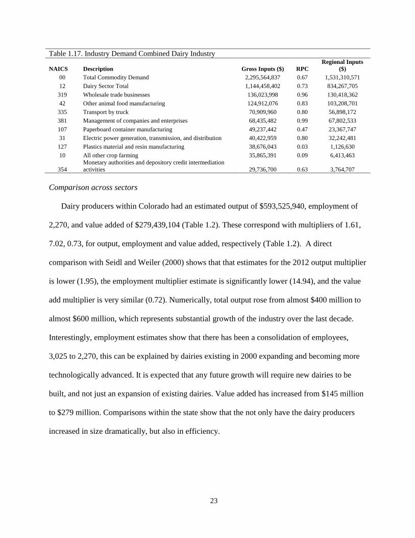
An analysis of the gross inputs for the dairy sector as a whole is reported in Table 1.17, which
indicates that of over $2 billion, 67% was sourced from local suppliers.
23
Table 1.17. Industry Demand Combined Dairy Industry
NAICS Description Gross Inputs ($) RPC
Regional Inputs
($)
00 Total Commodity Demand 2,295,564,837 0.67 1,531,310,571
12 Dairy Sector Total 1,144,458,402 0.73 834,267,705
319 Wholesale trade businesses 136,023,998 0.96 130,418,362
42 Other animal food manufacturing 124,912,076 0.83 103,208,701
335 Transport by truck 70,909,960 0.80 56,898,172
381 Management of companies and enterprises 68,435,482 0.99 67,802,533
107 Paperboard container manufacturing 49,237,442 0.47 23,367,747
31 Electric power generation, transmission, and distribution 40,422,959 0.80 32,242,481
127 Plastics material and resin manufacturing 38,676,043 0.03 1,126,630
10 All other crop farming 35,865,391 0.09 6,413,463
354
Monetary authorities and depository credit intermediation
activities 29,736,700 0.63 3,764,707
Comparison across sectors
Dairy producers within Colorado had an estimated output of $593,525,940, employment of
2,270, and value added of $279,439,104 (Table 1.2). These correspond with multipliers of 1.61,
7.02, 0.73, for output, employment and value added, respectively (Table 1.2). A direct
comparison with Seidl and Weiler (2000) shows that that estimates for the 2012 output multiplier
is lower (1.95), the employment multiplier estimate is significantly lower (14.94), and the value
add multiplier is very similar (0.72). Numerically, total output rose from almost $400 million to
almost $600 million, which represents substantial growth of the industry over the last decade.
Interestingly, employment estimates show that there has been a consolidation of employees,
3,025 to 2,270, this can be explained by dairies existing in 2000 expanding and becoming more
technologically advanced. It is expected that any future growth will require new dairies to be
built, and not just an expansion of existing dairies. Value added has increased from $145 million
to $279 million. Comparisons within the state show that the not only have the dairy producers
increased in size dramatically, but also in efficiency.
24
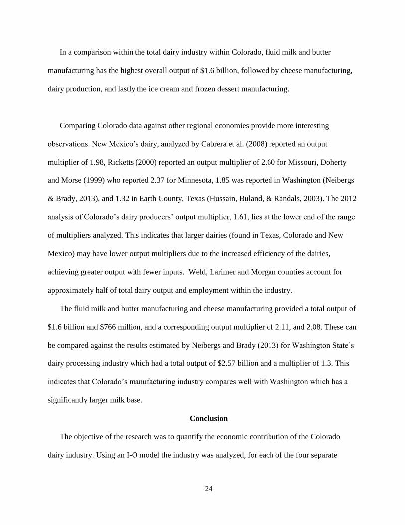
In a comparison within the total dairy industry within Colorado, fluid milk and butter
manufacturing has the highest overall output of $1.6 billion, followed by cheese manufacturing,
dairy production, and lastly the ice cream and frozen dessert manufacturing.
Comparing Colorado data against other regional economies provide more interesting
observations. New Mexico’s dairy, analyzed by Cabrera et al. (2008) reported an output
multiplier of 1.98, Ricketts (2000) reported an output multiplier of 2.60 for Missouri, Doherty
and Morse (1999) who reported 2.37 for Minnesota, 1.85 was reported in Washington (Neibergs
& Brady, 2013), and 1.32 in Earth County, Texas (Hussain, Buland, & Randals, 2003). The 2012
analysis of Colorado’s dairy producers’ output multiplier, 1.61, lies at the lower end of the range
of multipliers analyzed. This indicates that larger dairies (found in Texas, Colorado and New
Mexico) may have lower output multipliers due to the increased efficiency of the dairies,
achieving greater output with fewer inputs. Weld, Larimer and Morgan counties account for
approximately half of total dairy output and employment within the industry.
The fluid milk and butter manufacturing and cheese manufacturing provided a total output of
$1.6 billion and $766 million, and a corresponding output multiplier of 2.11, and 2.08. These can
be compared against the results estimated by Neibergs and Brady (2013) for Washington State’s
dairy processing industry which had a total output of $2.57 billion and a multiplier of 1.3. This
indicates that Colorado’s manufacturing industry compares well with Washington which has a
significantly larger milk base.
Conclusion
The objective of the research was to quantify the economic contribution of the Colorado
dairy industry. Using an I-O model the industry was analyzed, for each of the four separate

25
sectors within the Colorado dairy industry, dairy producers, fluid milk and butter manufacturers,
cheese manufactures, ice cream and frozen dessert manufacturers. After estimating the economic
contribution of each sector alone, the four individual components were aggregated into one
industry. The quantification of the industry allows for future policy decisions to be made with the
necessary knowledge, it provides an understanding of the social impact of the dairy industry,
details the impacts on related industry, and allows for the long term benefits of the industry to be
effectively analyzed. Primary results generated from the IMPLAN estimation were the total
output from each of the four industries; $593,525,940, $1,601,698,242, $766,750,610,
$61,544,628 respectively. This results in a combined economic contribution of over $3 billion to
the Colorado regional economy. Dairy producer industry created a total of 2,270 jobs in the
economy, fluid milk and butter manufacturing, 1,140, cheese manufacturing, 773, and ice cream
and frozen dessert manufacturing created a total of 150 jobs in the regional economy. The total
dairy industry combined to provide 4,333 jobs in the Colorado economy. For every $1 million
dollars of sales in the respective industries, it was estimated that 7.02 jobs would be created in
the dairy producers industry, 6.07 jobs in the fluid milk and butter manufacturing, 5.67 jobs in
the cheese manufacturing industry, and 7.51 jobs in the ice cream and frozen dessert industry.
The implications of this research are that there is room for growth in the dairy industry in
Colorado, and any additional growth in the dairy industry would be expected to benefit the
Colorado economy.
26
References
Balagtas, J. V., Hutchinson, F. M., Krochta, J. M., & Sumner, D. A. (2003). Anticipating
market effects of new uses for whey and evaluating returns to research and development. Journal
of dairy science, 86(5), 1662-1672.
Cabrera, V. E., Hagevoort, R., Solís, D., Kirksey, R., & Diemer, J. A. (2008). Economic
impact of milk production in the state of New Mexico. Journal of dairy science, 91(5), 2144-
2150.
Daniel, G., English, B. C., & Jensen, K. (2007). Sixty billion gallons by 2030: economic and
agricultural impacts of ethanol and biodiesel expansion. American Journal of Agricultural
Economics, 89(5), 1290-1295.
Day, F. & Minnesota IMPLAN Group (2013). Principles of Impact Analysis and IMPLAN
Applications. Minnesota IMPLAN Group Inc., Stillwater MN.
Doherty, B. A., Morse, G. W. (1999) Economic importance of Minnesota's dairy industry
.Ext. Serv. Bull. 07371. University of Minnesota, Minneapolis.
Gunter, A., Goemans, C., Pritchett, J. G., & Thilmany, D. D. (2012). Linking an Equilibrium
Displacement Mathematical Programming Model and an Input-Output Model to Estimate the
Impacts of Drought: An Application to Southeast Colorado. In 2012 Annual Meeting, August
12-14, 2012, Seattle, Washington (No. 124930). Agricultural and Applied Economics
Association.
Helmberger, P., & Chen, Y. H. (1994). Economic Effects of US Dairy Programs. Journal of
Agricultural & Resource Economics, 19(2).
Hjerpe, E. E., & Kim, Y. S. (2008). Economic impacts of southwestern national forest fuels
reductions. Journal of Forestry, 106(6), 311-316.
Hotvedt, J. E., Busby, R. L., & Jacob, R. E. (1988). Use of IMPLAN for regional input-
output studies. Buena Vista, Florida: Southern Forest Economic Association.
Houk, E. E., Frasier, W. M., & Schuck, E. C. (2004). The regional effects of waterlogging
and soil salinization on a rural county in the Arkansas River basin of Colorado. In Western
Agricultural Economics Association Meeting, Honolulu, HI.
Howe, C. W., & Goemans, C. (2003). Water Transfers and Their Impacts: Lessons from
Three Colorado Water Markets. JAWRA Journal of the American Water Resources
Association, 39(5), 1055-1065.
Hussain, S., Jafri, A., Buland, D., & Randals, S. (2003, April). Economic Impact of the Dairy
Industry in the Erath County, Texas. In Annual meeting of the Southwestern Social Sciences
Association, San Antonio, Texas.

27
Janssen, L., Taylor, G., Gerlach, M. E., & Garcia, A. (2006). Economic Impacts of
Alternative Sized Dairy Farms in South Dakota (No. 060001). South Dakota State University,
Department of Economics.
Leontief, W. W. (1936). Quantitative input and output relations in the economic systems of
the United States. The review of economic statistics, 105-125.
McKean, J. R., & Spencer, W. P. (2003). Implan understates agricultural input-output
multipliers: An application to potential agricultural/green industry drought impacts in
Colorado. Journal of Agribusiness, 21(2), 231-246.
Minnesota IMPLAN Group (2013). IMPLAN data for Colorado counties (2012). Minnesota
IMPLAN Group Inc., Stillwater MN.
Mon, P. N., & Holland, D. W. (2006). Organic apple production in Washington State: An
input–output analysis. Renewable Agriculture and Food Systems, 21 (02), 134-141.
Neibergs, J. S., & Brady, M. (2013). 2011 Economic Contribution Analysis of Washington
Dairy Farms and Dairy Processing: An Input-Output Analysis. School of Economic Sciences.
Washington State University Extension.
Pritchett, J., Thorvaldson, J., & Frasier, M. (2008). Water as a crop: Limited irrigation and
water leasing in Colorado. Applied Economic Perspectives and Policy, 30(3), 435-444.
Ricketts, R. (2000). Economic impact of the Missouri dairy industry. A strategic plan for
Missouri's dairy industry. University of Missouri, Columbia.
Seidl, A., & Weiler, S. (2000). Estimated economic impact of Colorado dairies. Department
of Agricultural and Resource Economics. Colorado State University Extension.
Watson, P., Wilson, J., Thilmany, D., & Winter, S. (2007). Determining economic
contributions and impacts: What is the difference and why do we care. Journal of Regional
Analysis and Policy, 37(2), 140-146.
Weiler, S., Loomis, J., Richardson, R., & Shwiff, S. (2002). Driving regional economic
models with a statistical model: hypothesis testing for economic impact analysis. The Review of
Regional Studies, 32(1), 97-111.
USDA. (2012) USDA/NASS Annual Milk Production, Disposition, and Income (PDI) and
Milk Production, various years. http://quickstats.nass.usda.gov/. Accessed March 2014.
28
Chapter 2:
Bringing Transparency to Class III Milk Futures: Evidence of Rational
Price Formation
Introduction
Dairy producers have faced increased volatility in milk prices over the last decade. This
increased uncertainty around revenues has added to management worries for dairy producers
who already face substantial variability in feed input costs. Class III milk prices are the most
traded contract of all futures contracts available to dairy producers, and as such are also the basis
of farm gate milk prices. With increasing uncertainty, a need has developed to bring some clarity
to the futures price evolution. There have been historically high levels of government
involvement in the pricing of dairy products; however, this is tapering off. As a result, milk
products are more responsive to supply and demand (Anderson & Ibendahl, 2000). With
increased market exposure, volatility has increased in the milk price market (Bozic, Newton,
Tharen, & Gould, 2012), coupled with increased volatility in feed inputs, producers have been
advised to manage risk more intensely. The use of hedging using futures contracts has been a
traditional risk management tool; however, trading volumes in the Class III milk futures contract
remains thin. Low trading volumes have been associated with a lack of knowledge of the market
and a lack of futures trading knowledge. To address some of the concerns of market participants,
a step is taken to bring more transparency to the Class III milk futures contracts by investigating
the presence of rational rice formation within the final year of a contracts life.

29
Literature Review
The United States (US) milk market does not fit into the standard competitive industry
mold. There have been numerous government programs which have altered the competitive
landscape through time. Dairy price support programs, import quotas on dairy products, and
federal milk marketing orders are examples of policy programs which have been implemented in
attempts to aid dairy farmers. Processed fluid milk and manufactured products are subject to
wholesale and retail price determination through the combined programs of price supports,
quotas, and marketing orders (Chouinard, Davis, LaFrance, & Perloff, 2010). This demonstrates
that the federal government has played a prominent role in the establishment of the farm value of
milk, or dairy pricing. Despite heavy government intervention in milk pricing, it is not the only
price determining method, market based pricing, similar to other agricultural commodity
products are also mechanisms for price discovery. Cash and futures markets located at the
Chicago Mercantile Exchange (CME), play key roles in price discovery.
The two predominant policy programs (sometimes called administered pricing programs)
currently implemented are the dairy product price support program (DPPSP) and federal milk
marketing orders (FMMOs) (Jesse and Cropp, 2008). The two policies originated sixty years ago
and have existed in various forms since their creation. They operate independently unless market
prices decline to such a point that support levels are breached. The DPPSP provides price support
for dairy farmers through government purchases of dairy products at legislated minimum prices
(Shields, 2009). Under the DPPSP policy, the federal government has the ability to purchase
unlimited amounts of butter, American cheese, and nonfat dry milk from dairy processors at
specified minimum prices. This creates a market floor price, and if prices drop to such a level,

30
the DPPSP program will begin purchasing product to support the price level and will continue
until the market price rises above the support price. However, when market prices are above
support levels, DPPSP does not factor in the market and milk pricing is based on supply and
demand (Shields, 2009).
The FMMO system was designed to stabilize market conditions and generally does not
support prices. The FMMP program was enacted during the 1920s and early 1930s when
volatility in market prices were at levels perceived to be too high. FMMOs mandate minimum
prices that processors in milk marketing areas must pay producers or their agents (e.g. dairy
cooperatives) for delivered milk depending on its end use, regardless of whether market prices
are high or low. Minimum milk prices are based on current wholesale dairy product prices
collected by USDA’s National Agricultural Statistics Service (NASS) in a weekly survey of
manufacturers, which are determined in large part by prices established on the CME (Shields,
2009). For this paper we are primarily concerned with Class III milk prices. The current Class III
milk FMMO program is derived using the following formula:
(1) 𝐶𝑙𝑎𝑠𝑠 𝐼𝐼𝐼 𝑝𝑟𝑖𝑐𝑒/𝑐𝑤𝑡
= 9.6396 𝑋 𝑁𝐴𝑆𝑆 𝑐ℎ𝑒𝑒𝑠𝑒 𝑝𝑟𝑖𝑐𝑒/𝑙𝑏 + 0.4199 𝑋 𝑁𝐴𝑆𝑆 𝑏𝑢𝑡𝑡𝑒𝑟 𝑝𝑟𝑖𝑐𝑒/𝑙𝑏
+ 5.8643 𝑋 𝑁𝐴𝑆𝑆 𝑑𝑟𝑦 𝑤ℎ𝑒𝑦 𝑝𝑟𝑖𝑐𝑒/𝑙𝑏 − 2.8189
The interpretation of the formula is as follows: a 10 cent-per-pound increase (decrease) in
cheese, butter, and dry whey prices will lead to an increase (decrease) the Class III price by 96.4,
42.0, and 58.6 cents per hundredweight, respectively. The combined make allowance, which is
built in manufacturing margin for processors, for cheese plants in this case is $2.82 per
hundredweight of milk used to make cheese (Jesse and Cropp, 2008). Therefore, as the FMMO
price is based on weekly USDA-NASS data, minimum prices rise and fall each month with

31
industry-wide changes in the dairy and dairy product market. Farmers receive a price for their
milk based on the minimum prices and on how their milk is utilized (fluid vs. manufacturing) in
the marketing order, which collectively is called “classified pricing”. FMMOs also address how
market profits are distributed among the producers delivering milk to federal marketing order
areas, called “pooling”, whereby all farmers receive a “blend price” each month based on order-
wide revenue. The blend price is the weighted average price in a marketing order, with the
weights being the volume of milk sold in each of the four classes6 (Shields, 2009).
Market based pricing in the dairy market works in the same manner as it would with
other commodities, generating current and future price level estimates for milk and dairy
products through competing bids from buyers and sellers who have different perceptions of
overall demand and supply conditions, along with expectations for changes in government
policy. Wholesale dairy product cash prices for cheese and butter are determined daily at the
CME during trading sessions that usually last only five minutes, nonfat dry milk on the other
hand also trades daily, but there is very little activity (Jesse and Cropp, 2008). These futures
prices are the basis of numerous contracts nationwide between dairy manufacturers and
wholesale or retail buyers of basic dairy products (Shields, 2009). Class III milk futures are the
primary drivers of farm prices as it is the single largest class use of milk and because Class I
(fluid) and Class II (soft manufactured product) minimum prices are established using Class III
prices. Class III futures and options are 200,000 pound monthly contracts that cash settle when
the Class III price is announced at the end of each month, contracts and options are available 24
months in advance (Wolf and Widmar, 2013).
6 Class I-Fluid, Class II-Soft Manufactured Product, Class III-Hard Cheeses and Cream Cheese, and Class IV-
Dry Milk Products and Butter

32
As we can see dairy pricing in the US is a combination of market-based and administered
(through public dairy programs) prices. Each influences the other to determine the overall price
level and price movements to some extent. In addition to the dynamics mentioned above,
perishability and year round daily production create challenges for pricing and marketing milk
and milk products (Shields, 2009). Dairy supply and demand also experience mismatched
seasonality, supply peaks in fall and demand is highest in January (Dong, Du, & Gould, 2011).
Despite the use of administered pricing policies, the dairy market has experienced
increased volatility in the Class III milk price. The volatility began after the 1970s and 1980s,
where dairy programs provided substantial price support. After a decrease in price support in the
mid-1980s volatility has increased on an annual basis ever since. A reduction in price support
and an increasing export dependent market are two primary drivers of increased volatility. Wolf
and Widmar (2013), using a monthly coefficient of variation to measure volatility, found that the
average monthly coefficient of variation from increased from 13.6% for the 1990 through 1999
time period to 20.4% for the period of 2000 to 2012 period. Open interest and volume traded of
Class III contracts have increased in the last 10 years (Wolf and Widmar, 2013), but are still very
small compared to other agricultural commodities.
The increased volatility has added another challenge to farmers who rely on futures
prices as a barometer of the market price for milk. In particular milk producers have faced
challenges effectively using them as indicators of future events, or in risk management strategies.
As a result of the heavy federal government involvement, market signals are not always
interpreted correctly, and can result in a delay in producers getting the information necessary to
33
make production decisions. Dairy farmers typically make production decisions based on price
received for their products, and will respond to prices by either reducing or increasing
production, if there is inefficiency in that price, production decisions will be adversely affected
resulting in an over or under supply of milk (Shields, 2009). The relatively large volatility of
Class III milk futures and the involvement of policy programs, may explain the lack of trading in
the futures market. This is counter-intuitive, as increased risk of revenue streams should prompt
producers to utilize hedging strategies more often, and also should entice speculators to the
market who benefit from volatility.
As noted earlier, there has been some increase in futures trading, but not by as much as
expected. Dairy farmers face risk related to output (milk) as well as feed costs (inputs), it is
critical that they manage both aspects of risk (Shields, 2009). With regard to using Class III
futures, some reasons for not trading in the futures market cited are lack of knowledge of futures
trading, lack of understanding of the market, and the reliance on existing dairy policies and or
cooperatives. Cooperatives are involved in risk management practices, including shifting
production between plants or product types in order to receive the highest return, integrating into
consumer and niche markets to diversify away from commodity market volatility, and forming
partnerships with other firms to shift business risk (Shields, 2009).
Malkiel and Fama (1970) described an efficient market as one that incorporates all
relevant and available information into the price. While another interpretation of an efficient
market is found in Working’s 1958 paper describing the theory of anticipatory prices, which
states that decisions on cash and futures prices take into account all available and relevant

34
information concerning historical relationships as well as current and expected supply-demand
conditions. From these definitions we can test for rational price formation in Class III milk
contracts by examining past price performance.
Koontz, Hudson, and Hughes, (1992) argue that futures contract prices reflect expected
market conditions when contracts are close enough to the delivery month that supply of the
underlying commodity cannot be changed. However, it is also stated that before this period of
“fixed-supply”, futures contract prices should be priced to reflect the competitive equilibrium, or
where output price equals average costs of production. The initial investigation into this line of
analysis was conducted by Tomek and Gray (1970), who identified two roles of futures markets
which are emphasized in the analysis of market performance. The first role, the allocative role,
was investigated by Working (1948) in a study of grain basis relationships and storage costs. In
the allocative role, availability of futures contracts for storable commodities, going out to a year
in the future, are thought to provide price incentives which influence storage decisions and
subsequently allocate grain consumption through the crop year. Analysis of the second role,
forward pricing, emerged with the futures trading in semi-storable commodities (e.g. onions and
potatoes) and nonstorable commodities (e.g. livestock). Price levels of futures contracts for
nonstorable commodities, deliverable up to 24 months in the future in the case of Class III milk
futures contracts, should forecast anticipated supply-demand conditions in these forward
markets. Futures markets for semi storable commodities (such as Class III milk futures) are
thought to combine these two roles (Koontz, Hudson, and Hughes, 1992).

35
Futures markets for seasonally produced commodities with continuous stocks are perhaps
the best known and best understood. In these markets the average cash price for a season
depends on the demand and supply conditions for the year, with monthly prices varying
seasonally around the average. Hence, a futures price for a particular delivery month depends
upon the expected average economic conditions for the year and upon conditions peculiar to that
month (Tomek and Gray, 1970). They suggest that futures markets for all commodities play both
roles, allocative and forward pricing, to some degree and that the storage characteristics of the
commodity determine the extent of each role. Therefore, for storable commodities, both roles are
played well, however, the role is primarily allocative, and by influencing storage decisions,
futures prices become self-fulfilling forecasts. For semi-storable commodities, the futures market
should play an allocative role across the time period that the crop is in storage (within the crop
year) but a forward pricing role across periods when the crop is not stored (across crop years).
Finally, for nonstorable commodities, such as livestock, the futures market should play a forward
pricing role (Koontz, Hudson, and Hughes, 1992). If the futures do not play these roles well,
then they would be inefficient and therefore participants in the futures market are not utilizing all
information available.
To determine whether Class III milk futures, a semi-storable commodity, follow this
price formation, we use the rational described by Koontz, Hudson, and Hughes, (1992), and
Dewbre, 1981 who use competitive market equilibrium conditions to examine if futures prices
follow a rational price formation process. The process implies that when a futures contract for a
nonstorable commodity is near maturity, the forward pricing role is consistent with rational price
formation, while further from maturity it will play more of an allocative role. Futures prices for

36
nearby contracts should reflect underlying supply and demand information as the information
becomes available. However, prior to committing the animals to feed, rational price formation
would suggest that the futures prices for distant and very distant contracts trade around expected
and then actual average costs of production. If futures contract prices reflect feeding costs, the
futures market is rational because it reflects competitive market equilibrium conditions.
The semi-storable nature of Class III milk futures are expected to show this distinction
between roles more clearly. The purpose of this paper is to provide an understanding of how
Class III contracts trade, and by providing transparency to the market, it is anticipated that
trading volume increases.
Model
The general model is based on research conducted by Koontz, Hudson, and Hughes,
(1992), where they test the rational price formulation theory proposed by Working (1948) and
Dewbre (1981). To begin this analysis, we determine a proxy for supply and demand (Equation
2) as well as feed cost equations (Equation 3) which will be included as independent variables in
the final regression used to test for evidence of rational pricing (Equation 4).
A set of 12 seemingly unrelated regressions were run to capture the effect of the
settlement price for a contract 𝑖 months from expiration from today 𝑡. Class III Milk futures
have 12 contracts (one for every month January – December) trading at any point in time, 𝑖 =
0, … ,11. Seemingly unrelated regressions accounted for the effect of supply and demand in the
last 12 months of a contracts life, before expiration. In Equation (2), 𝑆𝐷∗(𝑡+𝑖) is a proxy that
relates the effect that current, 𝑡, monthly supply and demand data, represented through an
equilibrium price or settlement price, have on all other open contracts that are 𝑖 months from

37
expiration. To account for seasonality within the demand functions dummy variables were
included, excluding January. Dummy variables are represented using the variable 𝐷.
(2) 𝑆𝐷∗(𝑡+𝑖) = 𝛽0 + ∑ 𝛽1
𝑖−1
𝑖=0
𝑆𝑃(𝑡+𝑖) + ∑ 𝛽2𝐷
11
𝑖=1
+ 𝜇𝑖
In contrast to the Koontz, Hudson, and Hughes, (1992) analysis which focused on beef
cattle and hogs in feedlot programs where feed costs make up 80-90% of variable costs, dairy
feeding costs are approximately 50-70% of variable costs (Bozic et al., 2012; Dhuyvetter, 2011).
However, despite feed costs not accounting for as large a percentage of variable costs as in the
beef and swine sectors, they were still the most prominent cost faced by producers (Wolf and
Widmar, 2013). Traders and producers also have the ability to forecast feed costs, allowing for
trading models to be built out.
In Equation (3), 𝐹𝐶∗𝐾 refers to the ration or feed cost in a given month 𝐾. 𝐹𝐶∗
𝐾 is a
function of 𝐹𝐶𝑡−𝑘 which represents feed cost in month 𝑘 prior to period 𝑡, where (𝑘 = 0, . . ,11).
A time trend variable is also incorporated using time squared values. Seasonality within
production is accounted for by using monthly dummy variables, which are all compared to
January as the base month. Again, 12 seemingly unrelated regressions were run, this accounted
for the 12 months of feed costs, i.e., feed costs for every month, in the last year of trading for any
give contract.
(3) 𝐹𝐶∗𝐾 = 𝛿1 + 𝛿2𝑡𝑖𝑚𝑒 + 𝛿3𝑡𝑖𝑚𝑒2 + ∑ 𝛿4𝐷
𝐾
𝑘=1
+ ∑ 𝛿5𝐴𝑅𝐽𝐹𝐴𝑡−𝑘
𝐾
𝑘=1
+ 𝜖𝑘
Equation (4) is the final equation in our system of equations, where 𝑆𝑃(𝑡+𝑖) refers to the
average monthly settlement price of the Class III Milk contract expiring in current month 𝑡 with 𝑖

38
months remaining for trade, 𝑖 (= 0,…, 11) signifying months prior to the delivery month7 in time
period 𝑡. 𝐹𝐶∗𝐾 refers to the aggregate U.S. feed costs per cwt for any given dairy producer in
month given by contract 𝑘 in time period 𝑡. While 𝑆𝐷∗(𝑡+𝑖) is a proxy of supply and demand in
the market, represented through the effect that the closing price of a contract in time 𝑡 with
𝑖 months remaining to delivery. In other words, Equation (4) illustrates that the settle price for a
contract in any given month prior to expiration is affected by the feeding costs in that month, and
the supply and demand conditions represented through the settlement price in time period 𝑡.
(4) 𝑆𝑃(𝑡+𝑖) = 𝛼0 + 𝛼1𝐹𝐶∗𝐾 + 𝛼2𝑆𝐷∗
(𝑡+𝑖) + 휀𝑘
The equations are defined as a contemporaneous system, where futures prices in a given
delivery month were modelled as a function of feeding costs and supply and demand conditions
in that month, and so on for months two to eleven. The contemporaneous system is thought to
provide evidence of rational price formation. The focus of this system is based on the
relationship between the feed and supply and demand variables and futures price during the
placement period. The settlement price and feed cost variable values should move together over
this time horizon and the relationship between the two variables should also expose the point at
which the relationship deteriorates. This deterioration is thought to occur in the nearby months,
during a period when the market views future supply of milk into the market as fixed, after this
point the supply and demand variable will move with the settlement price.
The necessary condition for rational price formation is that the estimated coefficient on
the cost variable is insignificantly different from one (𝛽1 = 1) in models where the time to
maturity of the futures price variable is greater than the length of the feeding period. In other
words, futures price should reflect costs in periods where supply decisions are flexible, and
7 Delivery month is the month in which the contract will expire or settle. For example a July 2015 contract, will
be delivered upon, or settle, or expire at the end of July in 2015.

39
subsequently reflect supply and demand conditions once they are perceived as fixed. However, if
rational price formation links futures prices to costs early in the contract life, and if, after the
placement period, futures prices symmetrically move above and below costs in the sample of
data, then the estimated cost coefficient may continue to be insignificantly different from one in
some nearby contract models. This means that even if the relationship between futures price and
variable costs is deteriorating, the tying of the futures prices to costs early in trading and to
symmetric price adjustments after the placement period may result in the appearance that prices
continue to move with costs during the nearby months.
Data
Data was collected from various sources to satisfy the requirements of Equation (2) and
(3). Settlement price (𝑆𝑃) was collected from the Understanding Dairy Markets web resource
(Gould, 2014), where daily announced Class III prices were collected from January 2001 to June
2013. The daily data was aggregated to monthly price averages, and the last day of the last
closing month of the contract was used as the settlement price. It is noteworthy, that the actual
announced price for Class III milk contracts were released on the first Friday following the
closing month of the contract, as this is when the FMMO price is released (Jesse and Cropp,
2008). The reasoning for using this price and not the announced price, was that volatility
decreased (Dong, Du, & Gould, 2011) due to the release of the weekly FMMO prices, and all
positions would have been made prior to the closing of the month. The data set yielded 150
observations.
Monthly ration/feed cost (𝐹𝐶∗) was developed using the Agricultural Reform, Food and
Jobs Act (ARFJA) Feed Ration as described by Bozic (2013). This ration was based on monthly

40
average national prices of corn, soybean meal and alfalfa hay as denoted in annual USDA
reports, the data collected covered the period January 2001 to June 2013 and is described by:
(5) 𝐴𝑅𝐹𝐽𝐴 = 1.0728 𝑥 𝐶𝑜𝑟𝑛 𝑃𝑟𝑖𝑐𝑒 + 0.00735 𝑋 𝑆𝑜𝑦𝑏𝑒𝑎𝑛 𝑀𝑒𝑎𝑙 𝑃𝑟𝑖𝑐𝑒+ 0.0137 𝑋 𝐴𝑙𝑓𝑎𝑙𝑓𝑎 𝐻𝑎𝑦 𝑃𝑟𝑖𝑐𝑒
Settlement price was used in both Equation (2) and (4), where is served as both a
regressand and a regressor. Feed cost data calculated by Equation (5) was used in Equation (3) as
the regressand.
Table 2.1 illustrates the summary statistics of all data used as inputs in Equations (2) and
(3) (where ARFJA Ration was described using Equation (5)). There were 150 observations for
all data collected, equating to monthly data points for the time period January 2001 to June 2013.
ARFJA Ration represents the calculated values based on Bozic, (2013) data, while the 12 groups
represented by 𝑖 = 0, … ,11, where 𝑖 are the months before the expiration month of a contract 𝑘.
These data show the ration cost for the month on a per hundredweight of milk basis. The mean
ration cost was approximately seven dollars, however a maximum ration cost, realized during
2012, peaked at over $15, while the minimum cost was less than $4. The wide range of feed
costs indicate how large an impact changing feed costs can have on a dairy producers’
profitability. Standard deviation of the values were similar for all data. Settlement Price (𝑖 =
0, … ,11) outlines a summary of the settlement price, or monthly average price that a contract
𝑘, would trade for the 12 months prior to expiration. The mean milk price over the period of
study was approximately $14, while the highest price received was over $21, and the lowest
price was close to $9. Standard deviation was higher closer to the expiration month and then
reduced. Again these milk price data indicate the high volatility present in the price of milk over
the period of study.
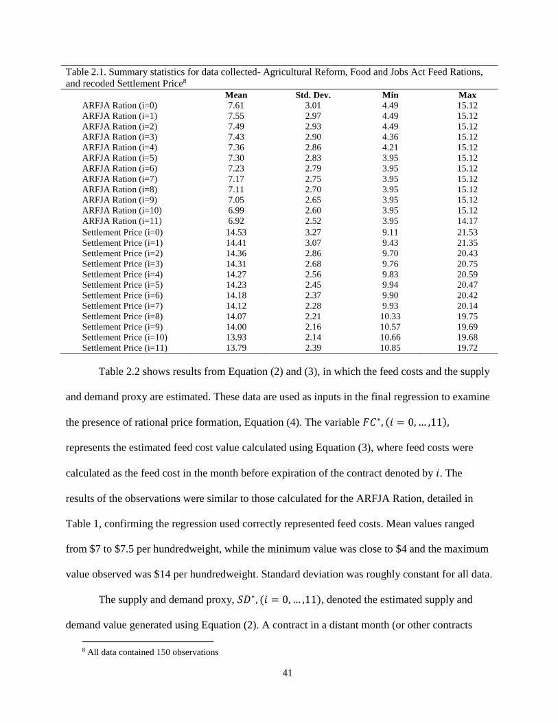
41
Table 2.1. Summary statistics for data collected- Agricultural Reform, Food and Jobs Act Feed Rations,
and recoded Settlement Price8
Mean Std. Dev. Min Max
ARFJA Ration (i=0) 7.61 3.01 4.49 15.12
ARFJA Ration (i=1) 7.55 2.97 4.49 15.12
ARFJA Ration (i=2) 7.49 2.93 4.49 15.12
ARFJA Ration (i=3) 7.43 2.90 4.36 15.12
ARFJA Ration (i=4) 7.36 2.86 4.21 15.12
ARFJA Ration (i=5) 7.30 2.83 3.95 15.12
ARFJA Ration (i=6) 7.23 2.79 3.95 15.12
ARFJA Ration (i=7) 7.17 2.75 3.95 15.12
ARFJA Ration (i=8) 7.11 2.70 3.95 15.12
ARFJA Ration (i=9) 7.05 2.65 3.95 15.12
ARFJA Ration (i=10) 6.99 2.60 3.95 15.12
ARFJA Ration (i=11) 6.92 2.52 3.95 14.17
Settlement Price (i=0) 14.53 3.27 9.11 21.53
Settlement Price (i=1) 14.41 3.07 9.43 21.35
Settlement Price (i=2) 14.36 2.86 9.70 20.43
Settlement Price (i=3) 14.31 2.68 9.76 20.75
Settlement Price (i=4) 14.27 2.56 9.83 20.59
Settlement Price (i=5) 14.23 2.45 9.94 20.47
Settlement Price (i=6) 14.18 2.37 9.90 20.42
Settlement Price (i=7) 14.12 2.28 9.93 20.14
Settlement Price (i=8) 14.07 2.21 10.33 19.75
Settlement Price (i=9) 14.00 2.16 10.57 19.69
Settlement Price (i=10) 13.93 2.14 10.66 19.68
Settlement Price (i=11) 13.79 2.39 10.85 19.72
Table 2.2 shows results from Equation (2) and (3), in which the feed costs and the supply
and demand proxy are estimated. These data are used as inputs in the final regression to examine
the presence of rational price formation, Equation (4). The variable 𝐹𝐶∗, (𝑖 = 0, … ,11),
represents the estimated feed cost value calculated using Equation (3), where feed costs were
calculated as the feed cost in the month before expiration of the contract denoted by 𝑖. The
results of the observations were similar to those calculated for the ARFJA Ration, detailed in
Table 1, confirming the regression used correctly represented feed costs. Mean values ranged
from $7 to $7.5 per hundredweight, while the minimum value was close to $4 and the maximum
value observed was $14 per hundredweight. Standard deviation was roughly constant for all data.
The supply and demand proxy, 𝑆𝐷∗, (𝑖 = 0, … ,11), denoted the estimated supply and
demand value generated using Equation (2). A contract in a distant month (or other contracts
8 All data contained 150 observations

42
being traded at the same time) is affected by the current month’s settlement price, and therefore
the supply and demand proxy represents the effect on contracts further from expiration, 𝑘.
Standard deviation in month 𝑘 was very low, which is expected due to only seasonal fluctuations
being taken into consideration in the seasonal month, however, standard deviations started higher
and then reduced further from expiration date. These values closely represent the settlement price
values, indicating the use of an efficient regression in Equation (2). The mean value was close to
$14.50, with a minimum value observed of less than $10, and a maximum value of close to $21.
The estimates generated, 𝐹𝐶∗ and 𝑆𝐷∗, were used as inputs in Equation (4) to produce an
estimated settlement price, where 𝑆𝑃∗, (𝑖 = 0, … ,11) represents the predicted values. These
estimated settlement prices can be compared to the actual collected Settlement Price, detailed in
Table 1. Mean values observed were around $14, while the minimum value was slightly below
$11, the maximum value was above $22. Standard deviations for these estimated values, do
indicated some potential issues. For contracts nine and ten months from expiration standard
deviations are low, indicating an issue with the data, which will be addressed later in the paper.
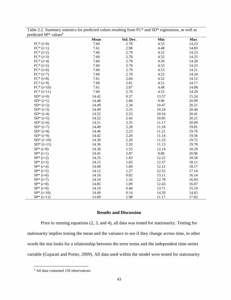
43
Table 2.2. Summary statistics for predicted values resulting from FC* and SD* regressions, as well as
predicted SP* values9
Mean Std. Dev. Min Max FC* (i=0) 7.60 2.78 4.53 14.23
FC* (i=1) 7.61 2.98 4.48 14.83
FC* (i=2) 7.60 2.79 4.52 14.23
FC* (i=3) 7.60 2.78 4.52 14.25
FC* (i=4) 7.60 2.78 4.50 14.28
FC* (i=5) 7.60 2.78 4.53 14.23
FC* (i=6) 7.60 2.79 4.53 14.21
FC* (i=7) 7.60 2.78 4.53 14.24
FC* (i=8) 7.61 2.84 4.52 14.12
FC* (i=9) 7.60 2.81 4.51 14.17
FC* (i=10) 7.61 2.87 4.48 14.08
FC* (i=11) 7.60 2.76 4.55 14.29
SD* (i=0) 14.42 0.57 13.57 15.24
SD* (i=1) 14.48 2.84 9.90 20.99
SD* (i=2) 14.49 2.34 10.47 20.21
SD* (i=3) 14.49 2.55 10.24 20.44
SD* (i=4) 14.52 2.53 10.54 20.41
SD* (i=5) 14.52 2.43 10.85 20.21
SD* (i=6) 14.51 2.35 11.17 20.09
SD* (i=7) 14.49 2.28 11.18 19.81
SD* (i=8) 14.46 2.23 11.21 19.76
SD* (i=9) 14.42 2.20 11.14 19.56
SD* (i=10) 14.39 2.20 11.23 19.72
SD* (i=11) 14.36 2.20 11.13 19.78
SP* (i=0) 14.38 1.55 12.14 18.29
SP* (i=1) 14.41 2.87 9.86 20.96
SP* (i=2) 14.25 1.83 12.22 18.58
SP* (i=3) 14.15 1.65 12.37 18.11
SP* (i=4) 14.08 1.69 12.12 18.17
SP* (i=5) 14.12 1.27 12.52 17.14
SP* (i=6) 14.16 0.82 13.11 16.14
SP* (i=7) 14.10 1.16 12.78 16.93
SP* (i=8) 14.85 1.09 12.43 16.07
SP* (i=9) 14.19 0.40 13.71 15.19
SP* (i=10) 14.49 0.14 14.20 14.65
SP* (i=11) 13.69 1.98 11.17 17.82
Results and Discussion
Prior to running equations (2, 3, and 4), all data was tested for stationarity. Testing for
stationarity implies testing the mean and the variance to see if they change across time, in other
words the test looks for a relationship between the error terms and the independent time-series
variable (Gujarati and Porter, 2009). All data used within the model were tested for stationarity
9 All data contained 150 observations

44
using the Augmented Dickey Fuller (ADF) test10. Results determined that the data set was
stationary and no adjustments needed to be made.
As mentioned previously, 12 models were calculated for Equation (2) and (3), this
allowed 12 seemingly related equations to be estimated for Equation (4), to reflect the 12 months
that the futures contracts would trade over 𝑖 = 0, … , 11. On the completion of generating
the 𝑆𝐷∗ and 𝐹𝐶∗ variables, an additional test was run to determine if the models exhibited serial
correlation, or “a lag correlation between two different series” (Gujarati and Porter, 2009). Serial
correlation in the case of our time series data would mostly likely be a problem of inertia, the
Cobweb Phenomenon, or lags in the data, leading to successive observations being
interdependent (Gujarati and Porter, 2009). This leads to the regressions not exhibiting efficient
estimators, potentially not allowing for the identification of significant coefficients,
underestimating the true variance, overestimating R2, and ultimately resulting in 𝑡 and 𝐹 tests no
longer being valid. The Durbin-Watson d-test11 was run to detect the presence of serial
correlation in the regressions. First-order serial correlation was found to be present in all three
equation systems. The regressions were corrected using the Prais-Winsten transformation
method, a generalized least-squares method to estimate the parameters in the regressions, the
transformed regressions were regressed in the difference form while maintaining the first
10 The ADF is used to test for stationarity and correct for correlation within the error term ∆𝑋𝑡 = 𝛿𝑋𝑡−1 + 𝜇𝑡.
𝑋𝑡 represents the various independent variables used in the model. Variables are regressed against the lagged values
of themselves, 𝑋𝑡−1 in addition to an error term 𝜇𝑡. Delta, 𝛿, is what the hypothesis test of the ADF test is analyzing.
The null hypothesis is that if delta is equal to zero then there exists a unit root and the variable is non-stationary. The
alternative hypothesis is that delta is greater than zero, meaning the time series is stationary. 11 The Durbin-Watson d statistic is simply the ratio of the sum of squared differences in successive residuals to
the RSS. 𝑑 =∑ (𝑢𝑡
𝑡=𝑛𝑡=2 −𝑢𝑡−1)2
∑ 𝑢𝑡2𝑡=𝑛
𝑡=1 .
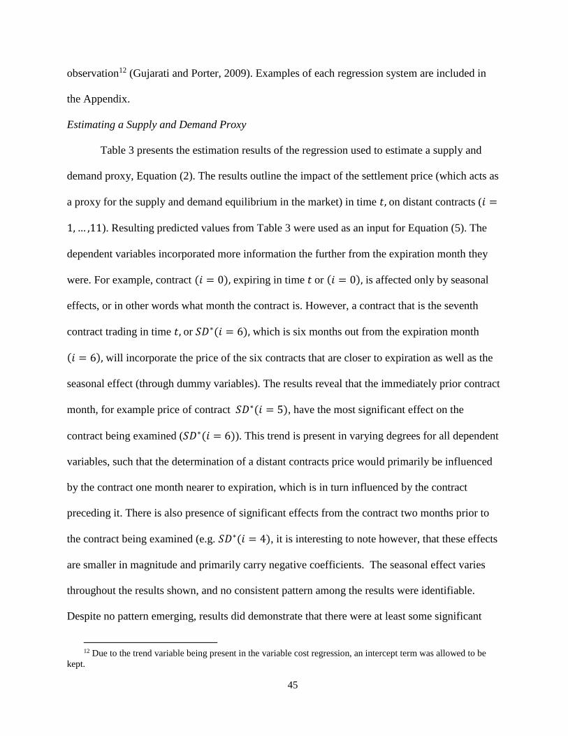
45
observation12 (Gujarati and Porter, 2009). Examples of each regression system are included in
the Appendix.
Estimating a Supply and Demand Proxy
Table 3 presents the estimation results of the regression used to estimate a supply and
demand proxy, Equation (2). The results outline the impact of the settlement price (which acts as
a proxy for the supply and demand equilibrium in the market) in time 𝑡, on distant contracts (𝑖 =
1, … ,11). Resulting predicted values from Table 3 were used as an input for Equation (5). The
dependent variables incorporated more information the further from the expiration month they
were. For example, contract (𝑖 = 0), expiring in time 𝑡 or (𝑖 = 0), is affected only by seasonal
effects, or in other words what month the contract is. However, a contract that is the seventh
contract trading in time 𝑡, or 𝑆𝐷∗(𝑖 = 6), which is six months out from the expiration month
(𝑖 = 6), will incorporate the price of the six contracts that are closer to expiration as well as the
seasonal effect (through dummy variables). The results reveal that the immediately prior contract
month, for example price of contract 𝑆𝐷∗(𝑖 = 5), have the most significant effect on the
contract being examined (𝑆𝐷∗(𝑖 = 6)). This trend is present in varying degrees for all dependent
variables, such that the determination of a distant contracts price would primarily be influenced
by the contract one month nearer to expiration, which is in turn influenced by the contract
preceding it. There is also presence of significant effects from the contract two months prior to
the contract being examined (e.g. 𝑆𝐷∗(𝑖 = 4), it is interesting to note however, that these effects
are smaller in magnitude and primarily carry negative coefficients. The seasonal effect varies
throughout the results shown, and no consistent pattern among the results were identifiable.
Despite no pattern emerging, results did demonstrate that there were at least some significant
12 Due to the trend variable being present in the variable cost regression, an intercept term was allowed to be
kept.

46
seasonal coefficients for all regressions run. The R2 value is very high from 𝑆𝐷∗(𝑖 = 1)
onwards, indicating that a contracts’ price in time 𝑡 is mostly explained by contracts closer to
expiration. The variable Rho indicates correlation between the variables, and can indicate the
presence of serial correlation within the observations. Table 2.3 results demonstrate that Rho
values are high in the expiration month, but are not an issue further out, which can be interpreted
as serial correlation not being a large issue.
Estimating Feed Cost
The results outlined in Table 2.4 are representative of Equation (3) which outlines the
estimated feed costs facing producers. Feed cost estimates were generated as a function of time
and season. Predicted values of feed costs were used as an input into Equation (4) as part of the
rational price formation analysis. Results from the estimation indicated that the time squared
variable was significant for all 12 regressions, however the magnitude of the coefficient was very
small. Seasonal effects of feed costs were present for all regressions, indicating the importance of
seasonal fluctuations within crop prices having a large impact on feed costs. It was interesting to
note that the seasonal impacts were never constant, a pattern emerged from the data that implied
in any given contract month, a minimum of four dummy variables would be significant, but the
months were different for each regression. Feed costs were included in the rational price
formation process, as they were the main costs faced by dairy producers, this estimation of feed
costs helps determine at which point the market perceives the supply of milk fixed. The presence
of serial correlation was detected in the data testing stage, and as previously described the Prais-
Winston correction was applied to all regressions. Despite this corrective procedure, it was noted
that the Rho values in Table 2.4 were close to 1, indicating the presence of serial correlation.
This was an unexpected result, and could have major consequences on any final results.

47
Table 2.3. OLS estimation results for the Supply and Demand proxy, using Equation (2) Dependent Variables
Independent Variables SD*(i=0) SD*(i=1) SD*(i=2) SD*(i=3) SD*(i=4) SD*(i=5)
SP (i=10)
SP (i=9)
SP (i=8)
SP (i=7)
SP (i=6)
SP (i=5)
SP (i=4)
1.402***
(0.09)
SP (i=3)
1.615*** -0.335**
(0.07) (0.15)
SP (i=2)
1.226*** -0.680*** 0.0101
(0.05) (0.11) (0.12)
SP (i=1)
0.883*** -0.334*** 0.0363 -0.0693
(0.04) (0.05) (0.06) (0.06)
SP (i=0)
0.905*** -0.117*** 0.0275 0.00954 -0.0288
(0.03) (0.04) (0.02) (0.02) (0.02)
Feb -0.205 0.36 -0.0416 0.11 0.0379 -0.0536
(0.34) (0.26) (0.11) (0.07) (0.08) (0.07)
Mar -0.0451 0.402 0.157 0.235** -0.0149 -0.161**
(0.46) (0.29) (0.15) (0.09) (0.08) (0.08)
Apr 0.228 0.44 0.382** 0.312*** -0.0418 -0.352***
(0.54) (0.30) (0.17) (0.10) (0.08) (0.08)
May 0.429 0.577* 0.529*** 0.179 -0.145* -0.631***
(0.59) (0.31) (0.18) (0.11) (0.08) (0.08)
Jun 1.128* 0.600* 0.450** 0.0453 -0.404*** -0.424***
(0.62) (0.31) (0.20) (0.12) (0.08) (0.09)
Jul 0.909 0.602* 0.567*** -0.267** -0.205** -0.436***
(0.63) (0.31) (0.20) (0.12) (0.09) (0.09)
Aug 1.434** 0.398 0.071 -0.132 -0.176** -0.415***
(0.62) (0.32) (0.20) (0.12) (0.08) (0.08)
Sep 1.462** 0.127 -0.113 -0.139 -0.281*** -0.163*
(0.60) (0.32) (0.19) (0.11) (0.08) (0.09)
Oct 1.284** -0.32 -0.142 -0.182* -0.0961 -0.140*
(0.55) (0.31) (0.18) (0.11) (0.08) (0.08)
Nov 0.711 0.135 -0.196 -0.0682 -0.0545 -0.220***
(0.48) (0.30) (0.15) (0.09) (0.08) (0.08)
Dec 0.652* -0.434 0.00764 0.00436 -0.0924 -0.161**
(0.36) (0.27) (0.12) (0.07) (0.08) (0.07)
Cons 13.77*** 1.112** 3.266*** 1.166*** 0.425*** 0.562***
(1.22) (0.43) (0.43) (0.24) (0.12) (0.13)
Obs 150 150 150 150 150 150
R-squared 0.1 0.895 0.885 0.964 0.993 0.991
Rho 0.919 0.286 0.815 0.665 0.092 0.188
Standard errors in parentheses
*** p<0.01, ** p<0.05, * p<0.1

48
Table 2.3. OLS estimation results for the Supply and Demand proxy, using Equation (2). Cont.. Dependent Variables
Independent Variables SD*(i=6) SD*(i=7) SD*(i=8) SD*(i=9) SD*(i=10) SD*(i=11)
SP (i=10)
1.345***
(0.09)
SP (i=9)
1.025*** -0.394***
(0.07) (0.13)
SP (i=8)
1.265*** 0.13 0.00317
(0.08) (0.12) (0.13)
SP (i=7)
1.374*** -0.18 -0.103 -0.0842
(0.09) (0.14) (0.12) (0.13)
SP (i=6)
1.145*** -0.476*** 0.0906 -0.310*** 0.137
(0.09) (0.14) (0.14) (0.11) (0.13)
SP (i=5) 1.317*** -0.0779 0.201 -0.301** 0.394*** 0.0623
(0.08) (0.15) (0.15) (0.14) (0.12) (0.13)
SP (i=4) -0.309** -0.13 -0.109 0.196 -0.139 -0.0675
(0.13) (0.14) (0.15) (0.14) (0.12) (0.12)
SP (i=3) 0.0213 0.198 -0.0255 0.00369 0.0477 -0.0378
(0.14) (0.15) (0.15) (0.14) (0.12) (0.13)
SP (i=2) -0.035 -0.134 0.0968 -0.188* -0.174* 0.105
(0.11) (0.11) (0.12) (0.11) (0.09) (0.10)
SP (i=1) -0.00618 -0.0729 -0.131** 0.0721 0.144*** -0.140***
(0.05) (0.06) (0.06) (0.06) (0.05) (0.05)
SP (i=0) -0.0148 0.0526** 0.0483** 0.0326 -0.0232 0.0582***
(0.02) (0.02) (0.02) (0.02) (0.02) (0.02)
Feb -0.0927 -0.246*** -0.0318 0.125* 0.0351 0.00181
(0.06) (0.07) (0.07) (0.07) (0.06) (0.06)
Mar -0.276*** -0.409*** -0.0443 0.237*** -0.0873 0.123
(0.07) (0.08) (0.09) (0.08) (0.07) (0.08)
Apr -0.491*** -0.417*** 0.00213 0.230** 0.0258 0.125
(0.08) (0.09) (0.11) (0.10) (0.08) (0.09)
May -0.385*** -0.301*** 0.0297 0.318*** 0.181** 0.189**
(0.09) (0.10) (0.11) (0.10) (0.09) (0.09)
Jun -0.351*** -0.241** 0.0998 0.473*** 0.211** 0.279***
(0.08) (0.10) (0.10) (0.10) (0.09) (0.10)
Jul -0.316*** -0.118 0.258** 0.409*** 0.213** 0.366***
(0.08) (0.10) (0.10) (0.10) (0.09) (0.09)
Aug -0.191** -0.00451 0.225** 0.431*** 0.287*** 0.420***
(0.08) (0.09) (0.09) (0.09) (0.08) (0.09)
Sep -0.128* -0.0884 0.278*** 0.621*** 0.282*** 0.324***
(0.08) (0.08) (0.09) (0.08) (0.09) (0.09)
Oct -0.171** -0.0375 0.434*** 0.531*** 0.227*** 0.126
(0.07) (0.08) (0.08) (0.09) (0.08) (0.09)
Nov -0.0457 0.0695 0.443*** 0.393*** 0.0172 -0.0156
(0.07) (0.08) (0.08) (0.08) (0.08) (0.08)
Dec 0.042 0.0438 0.261*** 0.165** -0.118** 0.0256
(0.07) (0.07) (0.07) (0.07) (0.06) (0.06)
Cons 0.566*** 0.420*** 0.137 -0.222 -0.0226 -0.0105
(0.13) (0.15) (0.16) (0.15) (0.14) (0.14)
Obs 150 150 150 150 150 150
R-squared 0.992 0.99 0.989 0.989 0.992 0.992
Rho 0.215 0.261 0.241 0.295 0.325 0.267
Standard errors in parentheses
*** p<0.01, ** p<0.05, * p<0.1
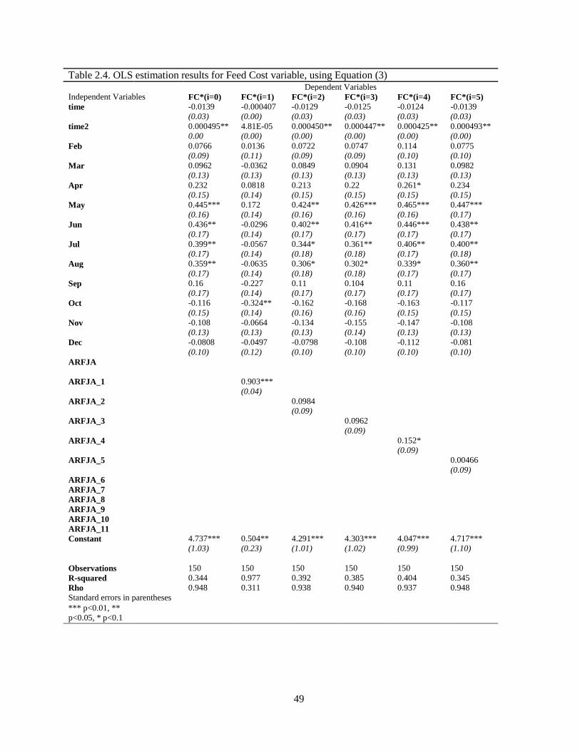
49
Table 2.4. OLS estimation results for Feed Cost variable, using Equation (3) Dependent Variables
Independent Variables FC*(i=0) FC*(i=1) FC*(i=2) FC*(i=3) FC*(i=4) FC*(i=5)
time -0.0139 -0.000407 -0.0129 -0.0125 -0.0124 -0.0139
(0.03) (0.00) (0.03) (0.03) (0.03) (0.03)
time2 0.000495** 4.81E-05 0.000450** 0.000447** 0.000425** 0.000493**
0.00 (0.00) (0.00) (0.00) (0.00) (0.00)
Feb 0.0766 0.0136 0.0722 0.0747 0.114 0.0775
(0.09) (0.11) (0.09) (0.09) (0.10) (0.10)
Mar 0.0962 -0.0362 0.0849 0.0904 0.131 0.0982
(0.13) (0.13) (0.13) (0.13) (0.13) (0.13)
Apr 0.232 0.0818 0.213 0.22 0.261* 0.234
(0.15) (0.14) (0.15) (0.15) (0.15) (0.15)
May 0.445*** 0.172 0.424** 0.426*** 0.465*** 0.447***
(0.16) (0.14) (0.16) (0.16) (0.16) (0.17)
Jun 0.436** -0.0296 0.402** 0.416** 0.446*** 0.438**
(0.17) (0.14) (0.17) (0.17) (0.17) (0.17)
Jul 0.399** -0.0567 0.344* 0.361** 0.406** 0.400**
(0.17) (0.14) (0.18) (0.18) (0.17) (0.18)
Aug 0.359** -0.0635 0.306* 0.302* 0.339* 0.360**
(0.17) (0.14) (0.18) (0.18) (0.17) (0.17)
Sep 0.16 -0.227 0.11 0.104 0.11 0.16
(0.17) (0.14) (0.17) (0.17) (0.17) (0.17)
Oct -0.116 -0.324** -0.162 -0.168 -0.163 -0.117
(0.15) (0.14) (0.16) (0.16) (0.15) (0.15)
Nov -0.108 -0.0664 -0.134 -0.155 -0.147 -0.108
(0.13) (0.13) (0.13) (0.14) (0.13) (0.13)
Dec -0.0808 -0.0497 -0.0798 -0.108 -0.112 -0.081
(0.10) (0.12) (0.10) (0.10) (0.10) (0.10)
ARFJA
ARFJA_1
0.903***
(0.04)
ARFJA_2
0.0984
(0.09)
ARFJA_3
0.0962
(0.09)
ARFJA_4
0.152*
(0.09)
ARFJA_5
0.00466
(0.09)
ARFJA_6
ARFJA_7
ARFJA_8
ARFJA_9
ARFJA_10
ARFJA_11
Constant 4.737*** 0.504** 4.291*** 4.303*** 4.047*** 4.717***
(1.03) (0.23) (1.01) (1.02) (0.99) (1.10)
Observations 150 150 150 150 150 150
R-squared 0.344 0.977 0.392 0.385 0.404 0.345
Rho 0.948 0.311 0.938 0.940 0.937 0.948
Standard errors in parentheses
*** p<0.01, **
p<0.05, * p<0.1
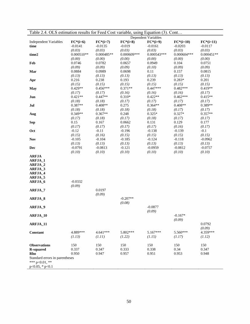
50
Table 2.4. OLS estimation results for Feed Cost variable, using Equation (3). Cont…
Dependent Variables
Independent Variables FC*(i=6) FC*(i=7) FC*(i=8) FC*(i=9) FC*(i=10) FC*(i=11)
time -0.0141 -0.0135 -0.019 -0.0161 -0.0203 -0.0117
(0.03) (0.03) (0.03) (0.03) (0.03) (0.03)
time2 0.000510** 0.000485** 0.000609*** 0.000543*** 0.000604*** 0.000451**
(0.00) (0.00) (0.00) (0.00) (0.00) (0.00)
Feb 0.0746 0.0782 0.0657 0.0949 0.104 0.0751
(0.09) (0.09) (0.09) (0.10) (0.09) (0.09)
Mar 0.0884 0.0989 0.0698 0.11 0.157 0.0815
(0.13) (0.13) (0.13) (0.13) (0.13) (0.13)
Apr 0.216 0.238 0.193 0.239 0.283* 0.201
(0.15) (0.15) (0.15) (0.15) (0.15) (0.15)
May 0.429** 0.456*** 0.371** 0.447*** 0.482*** 0.419**
(0.17) (0.17) (0.16) (0.16) (0.16) (0.17)
Jun 0.421** 0.447** 0.310* 0.422** 0.462*** 0.415**
(0.18) (0.18) (0.17) (0.17) (0.17) (0.17)
Jul 0.387** 0.408** 0.275 0.364** 0.408** 0.389**
(0.18) (0.18) (0.18) (0.18) (0.17) (0.17)
Aug 0.349** 0.367** 0.248 0.325* 0.327* 0.357**
(0.17) (0.18) (0.17) (0.18) (0.17) (0.17)
Sep 0.15 0.167 0.0662 0.131 0.129 0.177
(0.17) (0.17) (0.17) (0.17) (0.16) (0.17)
Oct -0.12 -0.11 -0.196 -0.138 -0.139 -0.1
(0.15) (0.16) (0.15) (0.15) (0.15) (0.15)
Nov -0.105 -0.104 -0.185 -0.124 -0.118 -0.0962
(0.13) (0.13) (0.13) (0.13) (0.13) (0.13)
Dec -0.0791 -0.0813 -0.121 -0.0959 -0.0812 -0.0757
(0.10) (0.10) (0.10) (0.10) (0.10) (0.10)
ARFJA
ARFJA_1
ARFJA_2
ARFJA_3
ARFJA_4
ARFJA_5
ARFJA_6 -0.0332
(0.09)
ARFJA_7
0.0197
(0.09)
ARFJA_8
-0.207**
(0.08)
ARFJA_9
-0.0877
(0.09)
ARFJA_10
-0.167*
(0.09)
ARFJA_11
0.0792
(0.09)
Constant 4.889*** 4.641*** 5.802*** 5.167*** 5.560*** 4.359***
(1.13) (1.11) (1.22) (1.15) (1.17) (1.12)
Observations 150 150 150 150 150 150
R-squared 0.337 0.347 0.333 0.338 0.34 0.347
Rho 0.950 0.947 0.957 0.951 0.953 0.948
Standard errors in parentheses
*** p<0.01, **
p<0.05, * p<0.1

51
Rational Price Formation
Table 2.3 and 2.4, have outlined the estimators which will be used as inputs into Equation
(4), which tests for the presence of rational price formation. Results are presented in a diagonal
format, so as to show each of the 12 seemingly unrelated regressions distinctly, the presentation
also allows for the time between each contract to be perceived correctly. For each regression
result, the dependent variable (e.g.𝑆𝑃 (𝑖 = 0)) was a function of the feed costs in that month,
(𝐹𝐶∗), and the supply and demand proxy, (𝑆𝐷∗(𝑖 = 0)), and each regression represents a
different month. The necessary condition for rational price formation is that the estimated
coefficient on the cost variable is insignificantly different from one (𝛽1 = 1). Theory also
indicates that the futures will play an allocative and forward pricing role in the lifetime of the
contract.
Results outlined in Table 2.5 provide evidence of rational price formation in Class III
milk futures contracts. The coefficient on feed costs is insignificantly different from one
at 𝑆𝑃 (𝑖 = 2), this implies that the market views the supply of milk as fixed from this period
onwards for a given contract. Further evidence of the rational price formation, is that the
coefficient on supply and demand is insignificant at 𝑆𝑃 (𝑖 = 1), indicating that the market is now
only taking into account the supply and demand information available on the market.
An interpretation of the feed cost coefficient becoming insignificantly different from one,
can be tied into dairy production practices through an examination of breeding practices. In a 12
month time horizon, cows are initially bred at 12 months of age and gestation is 9 month13. It is
assumed that the dairy cow will be integrated into the milking herd at the 10th month (provided
they are bred on the first try). This can be interpreted as the dairy producer views his production
13 On average a cow will give birth once every 12 months providing there are no delays in breeding.

52
fixed at the point of a cow entering the milking herd, at this point onwards feed costs associated
with that production would also be made and not change until that cow has to be bred again.
Results within Table 2.5 show that the Settlement Price of a contract in the distant
months follows the feed cost, or cost of production, in line with the competitive equilibrium
argument. Although Settlement Price is a function of feed costs in distant months, the
relationship does break down. An analysis of coefficients on 𝐹𝐶∗ show the coefficients
decreasing from 0.653 in 𝐹𝐶∗(𝑖 = 2), to 0.452 in 𝐹𝐶∗(𝑖 = 7), however the coefficients are still
highly statistically significant at this point. During this period when futures contract prices are
tracking the feed costs, the futures contract is said to be playing an allocative role. Once supply
is perceived as fixed, in 𝑆𝑃 (𝑖 = 1), the market focuses on supply and demand data, and it is said
the futures contracts play a forward pricing role, it is interesting to note that the forward pricing
role is only present for the last two months of a contract’s life.
A problem arises in the results when Rho is examined. The values of Rho, indicating
correlation are very high, signifying the presence of serial correlation. Serial correlation also
provides a potential explanation for the coefficients found on 𝐹𝐶∗(𝑖 = 8) and 𝑆𝐷∗(𝑖 = 8) where
the sign of the coefficient reverses. These two results, values of Rho and the change in
coefficient sign, indicate serial correlation is adversely affecting the results of Equation (4),
resulting in biased results.
An examination of the inputs reveals that feed costs are the primary driver of the serial
correlation that is present in Equation (4).

53
Table 2.5. OLS estimations for the presence of rational price formation through Equation (3)
Dependent Variables
Independent Variables SP (i=0) SP (i=1) SP (i=2) SP (i=3) SP (i=4) SP (i=5)
FC*(i=0) 0.531**
(0.26)
SD*(i=0) 0.830***
(0.28)
FC*(i=1)
0.0848**
(0.04)
SD*(i=1)
0.949***
(0.04)
FC*(i=2) 0.653***
(0.23)
SD*(i=2) 0.00344
(0.08)
FC*(i=3)
0.632***
(0.22)
SD*(i=3)
-0.0632
(0.08)
FC*(i=4) 0.716***
(0.20)
SD*(i=4) -0.170**
(0.07)
FC*(i=5)
0.562***
(0.20)
SD*(i=5)
-0.176**
(0.07)
FC*(i=6)
SD*(i=6)
FC*(i=7)
SD*(i=7)
FC*(i=8)
SD*(i=8)
FC*(i=9)
SD*(i=9)
FC*(i=10)
SD*(i=10)
FC*(i=11)
SD*(i=11)
Cons
-1.633 0.0349 9.232*** 10.26*** 11.11*** 12.41***
(4.51) (0.47) (2.00) (1.87) (1.77) (1.80)
Obs 150 150 150 150 150 150
R-squared 0.094 0.869 0.076 0.087 0.14 0.143
Rho 0.887 0.240 0.900 0.911 0.921 0.930
Standard errors in parentheses
*** p<0.01, ** p<0.05, * p<0.1
54
Table 2.5. OLS estimations for the presence of rational price formation through Equation (3). Cont..
Dependent Variables
Independent Variables SP (i=6) SP (i=7) SP (i=8) SP (i=9) SP (i=10) SP (i=11)
FC*(i=0)
SD*(i=0)
FC*(i=1)
SD*(i=1)
FC*(i=2)
SD*(i=2)
FC*(i=3)
SD*(i=3)
FC*(i=4)
SD*(i=4)
FC*(i=5)
SD*(i=5)
FC*(i=6) 0.369*
(0.21)
SD*(i=6) -0.126*
(0.07)
FC*(i=7)
0.452**
(0.17)
SD*(i=7)
-0.0535
(0.07)
FC*(i=8) -0.347
(0.25)
SD*(i=8) -0.0586
(0.08)
FC*(i=9)
0.182
(0.20)
SD*(i=9)
-0.0694
(0.08)
FC*(i=10) -0.0365
(0.21)
SD*(i=10) -0.0174
(0.08)
FC*(i=11)
0.452***
(0.12)
SD*(i=11)
0.377***
(0.14)
Cons 13.20*** 11.44*** 18.34*** 13.80*** 15.02*** 4.838***
(1.96) (1.68) (3.81) (2.32) (2.86) (1.48)
Obs 150 150 150 150 150 150
R-squared 0.122 0.168 0.044 0.107 0.064 0.091
Rho 0.944 0.933 0.991 0.975 0.988 0.582
Standard errors in parentheses
*** p<0.01, ** p<0.05, * p<0.1
Conclusion
The objective of the research was to test Class III milk pricing for the presence of rational
price formation. Through an analysis of Class III milk futures contracts 12 months before
expiration, an analysis of pricing rational takes place to determine whether the market is acting
efficiently. Theory suggests that contracts in distant months reflect market conditions, or feed
55
costs, but as the contract moves closer to expiration, the supply of the commodity becomes fixed
and the market price the contract according to the supply and demand dynamics affecting the
market. Using a system of 12 seemingly unrelated regressions, it is determined that Class III
milk futures contracts do follow rational pricing. Futures contracts are found to be acting in an
allocative capacity from 11 months to 3 months prior to expiration month. In the last 2 months,
the forward pricing role is dominant taking into account the supply and demand dynamics in the
market. If is found that Class III milk futures play both roles well, indicating that they are
efficient in utilizing all information available through the last 12 months of trading.
The implications of this study are that by creating a more transparent Class III futures
market it will entice more participants into the market. Increased trade within the market allows
for more effective hedging strategies, as speculators take on risk as opposed to producers.
Additional trading within the market allows for a more accurate price formation process to take
place as more information can be incorporated into the market through the different trading
strategies that individual traders may take. Through more trading, and more efficient price
determination, there is the potential for government involvement to decrease and allow a truly
competitive market to evolve.

56
References
Anderson, J. D., & Ibendahl, G. A. (2000). Risk management tools for dairy farmers: Options
on dairy futures. Cooperative Extension Service, College of Agriculture, University of Kentucky.
Bozic, M., Newton, J., Thraen, C. S., & Gould, B. W. (2012). Mean-reversion in income over
feed cost margins: Evidence and implications for managing margin risk by US dairy
producers. Journal of dairy science, 95(12), 7417-7428.
Bozic, M., Thraen, C.S. & Newton, J. (2013) “Managing Milk Price and Feed Cost Volatility
in the United States” in World Dairy Situation 2013 (in press)
Chouinard, H., Davis, D. E., LaFrance, J., & Perloff, J. M. (2010). Milk Marketing Orders:
Who Wins and Who Loses? Choices, 25(2).
Dewbre, J. H. (1981). Interrelationships between Spot and Futures Markets: Some
Implications of Rational Expectations. American Journal of Agricultural Economics, 63(5), 926-
933.
Dhuyveter, K., (2011). Factors Impacting Dairy Profitability: An Analysis of Kansas Farm
Management Association Dairy Enterprise Data. Department of Agricultural Economics, Kansas
State University.
Dong, F., Du, X., & Gould, B. W. (2011, July). Milk Price Volatility and its Determinants.
In AAEA and NAREA Joint Annual Meeting, Pittsburg (pp. 24-26).
Gould, B. W., (2014). Understanding Dairy Markets, Agricultural and Applied Economics,
UW Madison. http://future.aae.wisc.edu/
Gujarati, D. N., & Porter, D. C. (1999). Essentials of econometrics.Jesse, E., & Cropp, B.
(2008). Basic Milk Pricing Concepts for Dairy Farmers. Economic Research, 180, 200.
Koontz, S. R., Hudson, M. A., & Hughes, M. W. (1992). Livestock Futures Markets and
Rational Price Formation: Evidence for Live Cattle and Live Hogs. Southern Journal of
Agricultural Economics, 24, 233-233.
Malkiel, B. G., & Fama, E. F. (1970). Efficient capital markets: A review of theory and
empirical work*. The journal of Finance, 25(2), 383-417.
Shields, D. A., (2009) Dairy Pricing Issues. CRS Report to Congress #40903. Available at
http://www.nationalaglawcenter.org/assets/crs/R40903.pdf.
Tomek, W. G., & Gray, R. W. (1970). Temporal relationships among prices on commodity
futures markets: Their allocative and stabilizing roles. American Journal of Agricultural
Economics, 52(3), 372-380.
Wolf, C. A. (2012). Dairy farmer use of price risk management tools. Journal of dairy
science, 95(7), 4176-4183.

57
Wolf, C. A., Widmar, N. J. O., (2013) Adoption of Milk and Feed Forward-ricing Methods
by Dairy Farmers. Michigan State University, AgBioResearch
Working, H. (1948). Theory of the inverse carrying charge in futures markets. Journal of
Farm Economics, 30(1), 1-28.