CREDIT VALUE-AT-RISK UNDER TRANSITION PROBABILITY

(AN INTERAL RATING APPROACH)

BY

Badar-e-Munir

A thesis submitted in partial fulfillment of the requirements for the degree of

B.S Actuarial Science & Risk Management

Karachi University

2007

Approved by Mrs. Tahira Raza Chairperson of Supervisory Committee

Date 6-02-07

KARACHI UNIVERSITY

ABSTRACT

CREDIT VALUE-AT-RISK UNDER TRANSITION PROBABILITY

(AN INTERAL RATING APPROACH)

By Badar-e-Munir

Chairperson of the Supervisory Committee: Mrs. Tahira Raza

This paper gives the uses of numerical methods in rating based Credit Risk

Models. Generally such models use transition probabilities matrices to describe

probabilities from moving from one rating state to another rating state and then

calculate Value-At-Risk figures for portfolios. The value-at-risk framework is

used in model to calculate the maximum potential loss or expected loss of the

portfolio. However the several impediments to these measurements: a) credit risk

models deal with a default event for which one cannot assume simple

(logarithmic) normality and b) Data are subject to many constraints that will

reflect on many aspects of parameter estimation and setting, including default

rate, recovery rate and default correlation.

TABLE OF CONTENTS

Acknowledgments............................................................................................................... ii Glossary.............................................................................................................................. iiiii My Supervisor biography……………………………………………………... iv Chapter 1 Introduction…………………………………………………………….....01 Chapter 2 Rating Based Credit Risk Models…………………………………………..02 JLT Model……………………………………………………………..03 Cohort Model…………………………………………………………..03 Chapter 3 Applications of Credit Risk Models………………………………………...05 Chapter 4 Modelling Correlations…………………………………………………….06 Chapter 5 Probability Density Function of Credit Losses……………………………..07 Chapter 6 Credit Metrics Model……………………………………………………....08 Chapter 7 Value at Risk…………………………………………………………….....11 Chapter 8 Results………………………………………………………………….....13 Conclution……………………………………………………………………15 Appendix……………………………………………………………………..16 References

ii

ACKNOWLEDGMENTS

It is my pleasure to acknowledge the guidance and support of my thesis

supervisors: Mrs. Tahira Raza for her endless patience, encouragement, insight

and guidance and Mrs. Tahira Raza for giving me an opportunity and inspiring

me to succeed.

I would also like to acknowledge “National Bank of Pakistan”.

My deepest gratitude goes to all of my friends and family for their moral support,

understanding and help which allowed me to stay focused and maintains a good

quality of life during this process.

iii

Glossary

Basel II Basel II Capital Accord

CAR Capital Adequacy Ratio

IRB Advanced Internal Ratings Based Approach for

CR Credit risk

LGD Loss Given Default

M Maturity

PD Probability of Default

RWA Risk Weighted Assets

RAROC Risk Adjusted Return of Capital

EC Economic Capital

VaR Value at Risk

CVaR Credit Value at Risk

DM Default Mode

UL Unexpected Loss

EL Expected Loss

iv

MY SUPERVISOR BIOGRAPHY

Tahira Raza is currently working as head of risk review division at National Bank of Pakistan. She is a consummate banker and has worked at top level executive positions in various divisions of National Bank of Pakistan. In addition to MBA in finance from IBA (Karachi) she acquired DAIBP in which she secured 7 th position in Pakistan. Her versatile banking career spans over more than 30 years and features areas such as:

• Assets Liabilities Management • Credit Risk Modeling and Management • Credit Management • Micro Credit • Corporate and Consumer Loans • Basel II Implementation • Risk Rating Framework

For her contribution to the banking profession she has been awarded various honors such as:

• Selected as one of the two finalists for the position of FWBL President through interview process and recommended by the Finance Minster for final selection by the President of Pakistan in the Year 2001.

• Received Women Banker of the year 2006 Award from FPCCI Received best performance Award in Year 2006 by President NBP.

• Received best performance Award in Year 2005 by President NBP. • Best executive Award 1995 by President FWBL. • Best GM Award 1996 by President FWBL

She is a devoted professional banker and actively contributes through the forums such as the following:

• Member on a high powered Committee set up by Governor SBP for HR Development in banking sector.

• Member on a Committee to review and deliberate on prudential rules set by the central bank under the aegis of Pakistan Banks Association.

• Member of PBA’s committee on Basel II implementation. • Basel II Implementation. • Risk Rating Framework.

C h a p t e r 1

INTRODUCTION

Borrowing and lending money have been one of the oldest financial transactions. They are the core of the modern world’s sophisticated economy, providing funds to corporate and income to households. Nowadays, corporate and sovereign entities borrow either on the financial markets via bonds and bond-type products or they directly borrow money at financial institutions such as banks and savings associations. The lenders, e.g. Banks, private investors, insurance companies or fund Managers are faced with the risk that they might lose a portion or even all of their Money in case the borrower cannot meet the promised payment requirements. In recent years, to manage and evaluate Credit Risk for a portfolio especially so-Called rating based systems have gained more and more popularity. These systems Use the rating of a company as the decisive variable and not - like the formerly used So-called structural models the value of the firm - when it comes to evaluate the Default risk of a bond or loan. The popularity is due to the straightforwardness of the approach but also to the upcoming "New Capital Accord" of the Basel Committee on Banking Supervision, a regulatory body under the Bank of International Settlements, publicly known as Basel II. Basel II allows banks to base their capital Requirement on internal as well as external rating systems. Thus, sophisticated Credit risk models are being developed or demanded by banks to assess the risk of their credit portfolio better by recognizing the different underlying sources of Risk. Default probabilities for certain rating categories but also the probabilities for moving from one rating state to another are important issues in such Credit Risk Models. We will start with a brief description of the main ideas of rating-based Credit Risk Models and then give a survey on numerical methods that can be applied when it comes to estimating continuous time transition matrices or adjusting Transition probabilities.

2

C h a p t e r 2

RATING BASED CREDIT RISK MODELS

An Example

Source: Standard & Poor’s Credit Week (15 April 96)

3

THE JLT MODEL

Deterioration or improvement in the credit quality of the issuer is highly important for example if someone wants to calculate VaR figures for a portfolio or evaluate credit derivatives like credit spread options whose payouts depend on the yield spreads that are influenced by such changes. One common way to express these changes in the credit quality of market participants is to consider the ratings given by agencies like Standard & Poors and Moody`s. Downgrades or upgrades by the rating agencies are taken very seriously by market players to price bonds and loans, thus effecting the risk premium and the yield spreads. Jarrow/Lando/Turnbull (JLT) in 1997 constructed a model that considers different credit classes characterized by their ratings and allows moving within these classes. In this section, we will describe the basic idea of the the JLT model THE COHORT METHOD

In order to calculate transition probabilities from historical data, one can use the cohort method. The cohort method is most widely used and easy but, as will be shown, suffers an efficiency loss because of simplification. The cohort method assigns transition probabilities to every initial rating. It does so by using the relative frequencies of migration from historical data. It simply sums up the number of ratings in a certain state at the end of a period and divides it by the number of ratings at the beginning of the period. Table 1 shows the general construction for the corresponding transition matrix. Here pjk is the probability of migrating from state j to k. Let the total number of firms be N. Then in rating state j there are nj firms at the beginning of the period and njk migrated to state k at the end of the period. The estimated transition probability for stochastically independent migrations from initial rating j to k is: pjk = (njk / nj). The last row consists of zeros for all elements but the last one. This stems from the assumption that once an entity defaulted it will not leave this state again. Hence, the last row is identical for every possible transition matrix. Displaying the last row can therefore assumed to be optional. A transition matrix describes the probability of being in any of the various states in time T + 1 given state T. It is thus a full description of the probability distribution.

4

Table 1 : Probability for rating migration from rating j to K. The Cohort method for data has taken by Source: Credit Metrics Technical Document, the rating categories are assumed to be AAA, AA, A: and Default. The resulting matrix is (7x8) or, in the general case, (8-1) x 8 reflecting the absorbing property in the case of Default. That is the probability for leaving default once you defaulted is assumed to be zero. The entries in the first row of Table 2 show the behavior of initial AAA rated obligor's. A characteristic feature of rating transition matrices is the high probability mass on the diagonal. It shows that obligors are most likely to stay in their current rating.

AAA AA A BBB BB B CCC AAA 90.81% 0.70% 0.09% 0.02% 0.03% 0.01% 0.21%AA 8.15% 90.64% 2.27% 0.33% 0.14% 0.11% 0.23%A 0.68% 7.79% 91.05% 5.95% 0.67% 0.24% 0.35%BBB 0.12% 0.64% 5.52% 86.93% 7.73% 0.43% 1.30%BB 0.09% 0.06% 0.74% 5.30% 80.53% 6.48% 2.38%B 0.08% 0.14% 0.26% 1.17% 8.84% 83.46% 11.24%CCC 0.04% 0.02% 0.01% 0.12% 1.00% 4.07% 64.50%Default 0.03% 0.01% 0.06% 0.18% 1.06% 5.20% 19.79%

5

C h a p t e r 3

APPLICATIONS OF CREDIT RISK MODELS

Credit risk modeling methodologies allow a tailored and flexible approach to price measurement and risk management. Models are, by design, both influenced by and responsive to shifts in business lines, credit quality, market variables and the economic environment. Furthermore, models allow banks to analyze marginal and absolute contributions to risk, and reflect concentration risk within a portfolio. These properties of models may contribute to an improvement in a bank’s overall credit culture. The degree to which models have been incorporated into the credit management and economic capital allocation process varies greatly between banks. While some banks have implemented systems that capture most exposures throughout the organization, others only capture exposures within a given business line or legal entity. Additionally, banks have frequently developed separate models for corporate and retail exposures, and not all banks capture both kinds of exposures. The internal applications of model output also span a wide range, from the simple to the complex. For example, only a small proportion of the banks surveyed by the Task Force are currently using outputs from credit risk models in active portfolio management; however, a sizable number noted they plan to do so in the future. Current applications included: (a) setting of concentration and exposure limits; (b) setting of hold targets on syndicated loans; (c) risk-based pricing; (d) improving the risk/return profiles of the portfolio; (e) evaluation of risk-adjusted performance of business lines or managers using risk-adjusted return on capital (“RAROC”); and (f) economic capital allocation. Institutions also rely on model estimates for setting or validating loan loss reserves, either for direct calculations or for validation purpose.

6

C h a p t e r 4

MODELING CORRELATIONS

Credit metrics allows for correlated ratings transitions consists of assuming that each obligor’s ratings transitions are driven by a normally distributed

Portfolio management of credit risk cannot be performed in isolation without understanding the full impact of correlation on the portfolio. The movements in credit quality of different obligors are correlated; it is not prudent to set all correlations to zero, ignoring their implications for portfolio credit risk management. It must be kept in mind that the higher the degree of correlation, the greater is the volatility (i.e. unexpected loss) of a portfolio’s value attributable to credit risk. Since we are dealing with a DM approach, we are only interested in correlation of default occurrences. The portfolio by industry-specific information (industry sectors) and then calculating only the average default correlations within and between industry sectors. The asset returns correlation to quantify the default correlation, such as the Credit metrics model. In this latter case, using asset return correlation, we can obtain the default correlation of two discrete events over one year period based on the formula:

Where P1 and P2 are the probabilities of default for asset 1 and asset 2 respectively, while P1, 2 is the probability that both assets default.

7

C h a p t e r 5

PROBABILITY DENSITY FUNCTION OF CREDIT LOSSES

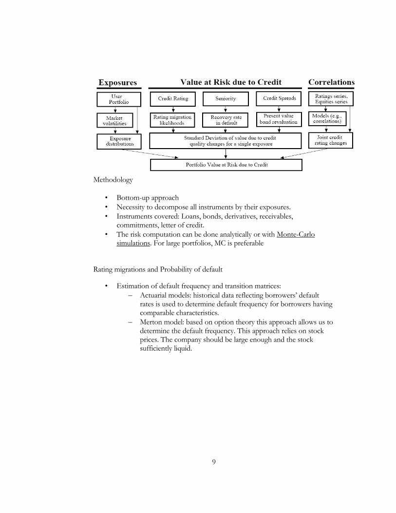
When estimating the amount of economic capital needed to support their credit risk activities, many large sophisticated banks employ an analytical framework that relates the overall required economic capital for credit risk to their portfolio’s probability density function of credit losses (PDF), which is the primary output of a credit risk model. A bank would use its credit risk modeling system (described in detail below) to estimate such a PDF. An important property of a PDF is that the probability of credit losses exceeding a given amount X (along the x-axis) is equal to the (shaded) area under the PDF to the right of X. A risky portfolio, loosely speaking, is one whose PDF has a relatively long and fat tail. The expected credit loss (shown as the left-most vertical line) shows the amount of credit loss the bank would expect to experience on its credit portfolio over the chosen time horizon. Banks typically express the risk of the portfolio with a measure of unexpected credit loss (i.e. the amount by which actual losses exceed the expected loss) such as the standard deviation of losses or the difference between the expected loss and some selected target credit loss quartile. The estimated economic capital needed to support a bank’s credit risk exposure is generally referred to as its required economic capital for credit risk. The process for determining this amount is analogous to value at risk (VaR) methods used in allocating economic capital against market risks. Specifically, the economic capital for credit risk is determined so that the estimated probability of unexpected credit loss exhausting economic capital is less than some target insolvency rate. Capital allocation systems generally assume that it is the role of reserving policies to cover expected credit losses, while it is that of economic capital to cover unexpected credit losses. Thus, required economic capital is the additional amount of capital necessary to achieve the target insolvency rate, over and above that needed for coverage of expected losses. A target insolvency rate equal to the shaded area, the required economic capital equals the distance between the two dotted lines. Broadly defined, a credit risk model encompasses all of the policies, procedures and practices used by a bank in estimating a credit portfolio’s PDF.

8

C h a p t e r 6

CREDIT METRICS MODEL

The three major drivers of the portfolio credit risk are the probability of default, loss given default, and correlations. Credit Metrics is a one-period, rating-based model that uses the simulation of multiple normally distributed risk factors to yield a Credit value at risk. To compute the probability of default inputs, the rating (e.g AA) and horizon there is a probability of transition to another rating. Using calculated transition matrices, the probability of a position moving from its current rating to a rating that indicates default. The Gathering of Inputs: This step includes calculating many measures such as probabilities of default, recovery rates statistics, factor correlations and their relationships to the obligors, yield curve data and individual exposures that are distinct from the other inputs. Generating Correlated Migration Events: This step attempts to measure the extent to which the debt positions will tend to experience a similar rating change or transitions (e.g the probability that two investment grade bonds will both be down graded to non investment grade). Measuring “Marked to Model” losses: The results from step 2 can generate simulations that give profits or losses from the transition. For simulated values that correspond to default, the procedure would compute a recovery rate using the beta distribution for non default firms in the simulation; forward curves estimate the value of the positions. Calculating the Portfolio loss distribution: This is done by comparing the current value of the portfolio to the estimate of the terminal value, which is the sum of all the forward values of the positions. A distribution terminal value is computed using different values of the risk factors. This distribution is used to compute Value at Risk (VaR) and different risk measure.

9

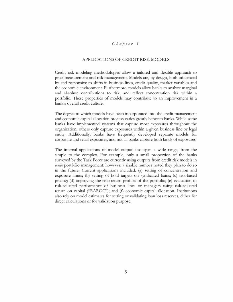
Methodology

• Bottom-up approach • Necessity to decompose all instruments by their exposures. • Instruments covered: Loans, bonds, derivatives, receivables,

commitments, letter of credit. • The risk computation can be done analytically or with Monte-Carlo

simulations. For large portfolios, MC is preferable Rating migrations and Probability of default

• Estimation of default frequency and transition matrices: – Actuarial models: historical data reflecting borrowers’ default

rates is used to determine default frequency for borrowers having comparable characteristics.

– Merton model: based on option theory this approach allows us to determine the default frequency. This approach relies on stock prices. The company should be large enough and the stock sufficiently liquid.

10

Correlations among defaults

• Correlations between credit events (default or migration) are an important input data.

• Credit defaults or migration are not independent events but present correlations.

• Assessing correlation is not an easy task. There are two main possible approaches:

– Actuarial methods – Equity-based methods

• Lack of data is an issue (this is a general issue in credit risk models) • It is difficult to assess the sensitivity of risk metrics to the error in

correlations. • Model sensitivity to correlations (and all other key parameters!) should be

tested. Key concepts in Credit Risk Modeling

• Probability Density Function (PDF) of credit losses: – This is the main output of credit risk models. – Allows us to determine: EL, UL, economic capital to cover

• Expected loss gives the “average” loss expected to occur over the model’s time horizon.

• Portfolio risk is measured by unexpected loss. • UL gives the measure of allocated economic capital

11

C h a p t e r 7

VALUE – AT - RISK

To assess the performance of different credit risk models, we compare VaR measures for a one-year holding period with the actual outturns of different portfolios. These comparisons are complicated, however, by the fact that the model described above abstracts from interest volatility in calculating risk measures. To see how well the model measures credit risk, one must, therefore, remove from the portfolio value realization that part of the value change that is attributable to changes in the default-free term structure. The empirical distribution generated by the credit risk model indicates that for

some confidence level, c, Probt (PT < γ ) = c for a cut-o point or ‘VaR

quantile’, γ , then we can compare the return in equation with the quantity:

Then the loss on the position has exceeded the VaR. γ can be directly deduced from the portfolio value empirical distribution or by assuming normality. In this case, the 99% VaR, may be calculated by inverting the probability statement:

To obtain:

12

Where µp and σp are the portfolio’s analytical mean and volatility.

13

C h a p t e r 8

RESULTS

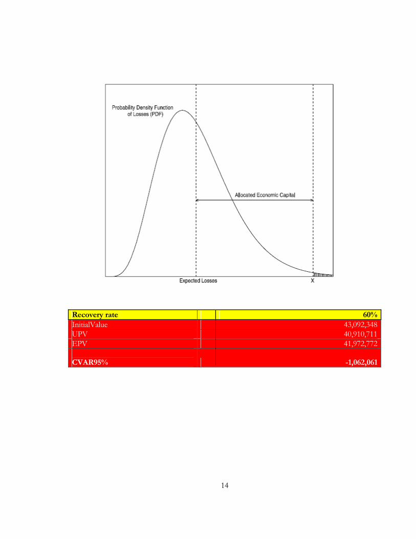
The VaR estimate is based on a one-year holding period and a 99% confidence level. The Basel Committee on Banking Supervision (1996), an exception occurs when the outturn loss on a portfolio exceeds the VaR measure supplied by a VaR model. Such an exception takes place when the solid line representing year-on-year return fall below one of the VaR levels. If the Credit risk models were correctly measuring risk, and we had non-overlapping observations. VaRs derived from a Monte Carlo generated portfolio distribution for various values and for a 10% recovery rate in the case of default. The VaR level and the number of exceptions are highly sensitive to the choice ofα. The obligors in our sample for which we have equity prices estimate a as the correlation between the firm’s equity. The average Monte Carlo VaR with the VaR derived by assuming that portfolio values are normally distributed. The large difference between the two risk measures is due, as one should expect, to the pronounced negative skew ness and leptokurtosis of loan portfolio distributions, caused by the potentially large downfalls that follow default events.

14

Recovery rate 60%InitialValue 43,092,348UPV 40,910,711EPV 41,972,772 CVAR95% -1,062,061

15

CONCLUSION In this paper, I conduct the first out-of-sample evaluation of a new type of credit risk models. The model we study derives risk estimates for a portfolio of credit exposures by exploiting the information embedded in the exposures’ credit rating. The most important feature of the new methodology is to provide a way to model the correlation of rating migrations. Approach consists of implementing the model over a five to eight year period on large portfolios. Month-by-month, we calculate the risk measures implied by the model and compare them with the actual outcomes as credit spreads move around. I conclude that a standard implementation of the model may lead to several underestimations of portfolio risk. We find this problem can be eased by using conservative parameterizations. Results suggest that it would be prudent to build in safety margin into capital allocation decisions and regulatory capital calculations if at a future date they were based on output from the current generation of rating-based credit risk models.

16

APPENDIX

DATA For the current research I used the data from Credit Metrics Technical Document. TRANSITION MATRIX

AAA AA A BBB BB B CCC AAA 90.81% 0.70% 0.09% 0.02% 0.03% 0.01% 0.21%AA 8.15% 90.64% 2.27% 0.33% 0.14% 0.11% 0.23%A 0.68% 7.79% 91.05% 5.95% 0.67% 0.24% 0.35%BBB 0.12% 0.64% 5.52% 86.93% 7.73% 0.43% 1.30%BB 0.09% 0.06% 0.74% 5.30% 80.53% 6.48% 2.38%B 0.08% 0.14% 0.26% 1.17% 8.84% 83.46% 11.24%CCC 0.04% 0.02% 0.01% 0.12% 1.00% 4.07% 64.50%Default 0.03% 0.01% 0.06% 0.18% 1.06% 5.20% 19.79%

RATING MIGRATION THRESHOLD

AAA AA A BBB BB B CCC AAA #NUM! #NUM! #NUM! #NUM! #NUM! #NUM! #NUM! AA -1.32915 2.457263 3.121389 3.540084 3.431614 3.719016 2.862736A -2.3116 -1.36199 1.984501 2.696844 2.92905 3.035672 2.619728BBB -2.68745 -2.37814 -1.50704 1.530068 2.391056 2.687449 2.413503BB -2.82016 -2.83379 -2.30085 -1.49314 1.367719 2.413503 2.035506B -2.96774 -2.92905 -2.71638 -2.17808 -1.23186 1.455973 1.698571CCC -3.19465 -3.43161 -3.19465 -2.74778 -2.04151 -1.32431 1.006448Default -3.43161 -3.71902 -3.23888 -2.91124 -2.3044 -1.62576 -0.84915

CORRELATION MATRIX (BETWEEN INDICES SECTORS)

1 2 3 4 5 6 7 8 9 10 11 12 13 14 15 16 17 18 19 20

1 1 0.45 0.45 0.45 0.15 0.15 0.15 0.15 0.15 0.15 0.1 0.1 0.1 0.1 0.1 0.1 0.1 0.1 0.1 0.12 0.45 1 0.45 0.45 0.15 0.15 0.15 0.15 0.15 0.15 0.1 0.1 0.1 0.1 0.1 0.1 0.1 0.1 0.1 0.13 0.45 0.45 1 0.45 0.15 0.15 0.15 0.15 0.15 0.15 0.1 0.1 0.1 0.1 0.1 0.1 0.1 0.1 0.1 0.14 0.45 0.45 0.45 1 0.15 0.15 0.15 0.15 0.15 0.15 0.1 0.1 0.1 0.1 0.1 0.1 0.1 0.1 0.1 0.15 0.15 0.15 0.15 0.15 1 0.35 0.35 0.35 0.35 0.35 0.2 0.2 0.2 0.2 0.2 0.2 0.2 0.15 0.1 0.16 0.15 0.15 0.15 0.15 0.35 1 0.35 0.35 0.35 0.35 0.2 0.2 0.2 0.2 0.2 0.2 0.2 0.15 0.1 0.17 0.15 0.15 0.15 0.15 0.35 0.35 1 0.35 0.35 0.35 0.2 0.2 0.2 0.2 0.2 0.2 0.2 0.15 0.1 0.18 0.15 0.15 0.15 0.15 0.35 0.35 0.35 1 0.35 0.35 0.2 0.2 0.2 0.2 0.2 0.2 0.2 0.15 0.1 0.19 0.15 0.15 0.15 0.15 0.35 0.35 0.35 0.35 1 0.35 0.2 0.2 0.2 0.2 0.2 0.2 0.2 0.15 0.1 0.110 0.15 0.15 0.15 0.15 0.35 0.35 0.35 0.35 0.35 1 0.2 0.2 0.2 0.2 0.2 0.2 0.2 0.15 0.1 0.111 0.1 0.1 0.1 0.1 0.2 0.2 0.2 0.2 0.2 0.2 1 0.5 0.5 0.5 0.5 0.2 0.2 0.2 0.1 0.112 0.1 0.1 0.1 0.1 0.2 0.2 0.2 0.2 0.2 0.2 0.45 1 0.5 0.5 0.5 0.2 0.2 0.2 0.1 0.113 0.1 0.1 0.1 0.1 0.2 0.2 0.2 0.2 0.2 0.2 0.45 0.5 1 0.5 0.5 0.2 0.2 0.2 0.1 0.114 0.1 0.1 0.1 0.1 0.2 0.2 0.2 0.2 0.2 0.2 0.45 0.5 0.5 1 0.5 0.2 0.2 0.2 0.1 0.115 0.1 0.1 0.1 0.1 0.2 0.2 0.2 0.2 0.2 0.2 0.45 0.5 0.5 0.5 1 0.2 0.2 0.2 0.1 0.116 0.1 0.1 0.1 0.1 0.15 0.15 0.15 0.15 0.15 0.15 0.2 0.2 0.2 0.2 0.2 1 0.6 0.55 0.25 0.2517 0.1 0.1 0.1 0.1 0.15 0.15 0.15 0.15 0.15 0.15 0.2 0.2 0.2 0.2 0.2 0.6 1 0.55 0.25 0.2518 0.1 0.1 0.1 0.1 0.15 0.15 0.15 0.15 0.15 0.15 0.2 0.2 0.2 0.2 0.2 0.6 0.6 1 0.25 0.2519 0.1 0.1 0.1 0.1 0.1 0.1 0.1 0.1 0.1 0.1 0.1 0.1 0.1 0.1 0.1 0.3 0.3 0.25 1 0.6520 0.1 0.1 0.1 0.1 0.1 0.1 0.1 0.1 0.1 0.1 0.1 0.1 0.1 0.1 0.1 0.3 0.3 0.25 0.65 1

UNCORRELATED RANDOM VARIABLES 1 2 3 4 5 6 7 8 9 10 11 12 13 14 15 16 17 18 19 20

1 0.38704 1.2 0.55 -1 -0.3 -1.5 -0.9 1.96 -0.4 0.17 0.72 -0.4 -2.5 1 -2.8 -0.1 0.59 1.7 1.1 0.42 0.95206 -0.4 0.03 -0.3 -0.1 -1 -0.3 3.08 1.4 2.21 1.55 0.13 0.8 1.24 -0.7 -0.1 0.37 -0.1 -0.7 0.43 0.26726 -0.3 -0 -0.6 0.96 -0.7 -0.9 1.94 -0.3 1.53 0.87 -0.4 -0.3 -1.1 -0.9 0.6 -0.7 -0.3 0.7 -0.44 0.14204 -1.4 0.11 1.2 0.76 -1 0.2 -0.9 0.4 0.1 -1.6 -1.2 0.1 -0.5 1.2 0.4 0.94 0 1.8 1.35 -0.4824 -0.4 -1.1 -1.2 1.09 -1.4 2 -0.8 0.2 -1.7 -0.6 2.22 1.6 0.56 0.3 -0.7 -0.5 -0.5 0.9 -0.26 -3.4781 -0.1 -1.2 -0.8 0.49 2.58 -1.2 1.37 0.7 -1.5 -0.3 -0.2 -1 1.35 -0.6 -1 -1 1 0.7 0.97 1.65187 0.2 1.18 -0.2 -1.3 -0.8 0.7 -0.7 1.3 -0.2 -0 -0.5 1.1 0.01 -1.1 1 2.6 1.9 -1.9 -08 0.18493 0 0.68 -1 -1 -1.8 1.2 0.43 1.1 1.37 0.34 -1.2 -0.8 -0.6 0.7 -0.9 0.57 0.7 0.9 -0.29 -2.3062 0.9 -0.6 1.31 -0.6 -1.6 -0.7 0.41 0.3 2.02 -0.4 0.28 -0.9 1.05 0.8 -0.5 0.6 1.2 0.7 -2

10 -0.6575 -0.2 0.14 0.16 0.24 -1.1 -0.3 -1.6 1 -2.4 -0.4 0.57 1 0.39 -0.6 1.3 -0.4 3.8 0.3 -0.6

. . . . . . . . . . . . . . . . . . . . .

. . . . . . . . . . . . . . . . . . . . .

. . . . . . . . . . . . . . . . . . . . .

. . . . . . . . . . . . . . . . . . . . .

. . . . . . . . . . . . . . . . . . . . .9993 -0.6387 -1.7 0.6 0.07 -0.7 -0.8 -1.5 0.01 0.4 0.39 -1.5 -0.4 -0.8 0.89 -1.5 -0.6 1.04 -0.5 0.3 0.29994 0.74031 0.4 0.67 1.08 -1 -1.1 -0.4 0.08 0 0.37 -1.8 -0.3 -0.6 -0.4 -0.2 0 0.05 -0.1 0.9 -0.49995 -0.9279 0.6 -0.7 1.83 0.6 -0.1 -0.9 1.46 -0.6 0.58 -0.1 0.27 0.1 0.48 1 -0.2 -1.9 -0.7 -0.9 -0.29996 0.68843 -0.4 0.23 0.73 -0.1 1.29 -0.6 0.72 -1.2 0.01 1.77 -0.1 -1 0.32 0.9 -0.7 -1 -0.8 -0 -19997 -0.0808 0.1 1.57 -1.6 0.42 0.83 -1.6 1.18 0.6 -0.4 -1.4 -1.1 1.6 -0.2 0.6 0.2 0.12 0.3 -0.5 1.4

2

9998 1.61606 2.9 -2.6 -0 2.08 -1 -0.7 -1.2 -0.2 0.74 0.36 0.84 -2.1 -1.4 0.3 1.5 -0.4 -0.6 -1.2 0.79999 0.89286 -0.3 -2.4 -0.3 -0.9 0.41 0.7 0.73 0.9 0.7 -0.2 0.43 -0.9 0.87 0.8 -0.9 1.08 0.4 1.6 0.2

10000 1.45237 1 2.87 0.07 0.17 0.27 0.9 -1.8 0.1 -1 0.57 2.22 -0.6 0.2 0.5 0.8 1.18 0.7 2.1 0.8

3

MIGRATIONS SIMULATED

Rating AAA AA AA AA AA AA A A A A BBB BBB BBB BBB BBB BB BB B B CCC

Asset # 2 1 7 8 9 13 4 10 11 20 6 14 15 16 17 3 12 5 19 18

AAA AA AA AA AA A A A A A BBB BBB BB BBB f BB BB B B B AAA AA AA AA AA AA A AA A AA A BBB A A BBB BB BB B B CCC AAA AA AA AA AA AA A A A A BBB BBB BBB BBB BBB BB BB B B CCC AAA AA AA AA AA AA A A A A BB BB BBB BBB BBB BB BB B BB Default AAA AA AA A AA AA A A A A BBB A A BBB BBB BB BB B B CCC Default A BBB BBB AA AA A A A A BBB BBB BBB BBB BBB B B B B CCC AAA AA AA AA AA AA A A A A BBB BBB BBB BBB BBB BB A A B CCC AAA AA AA AA AA A A A A A BBB BBB BBB BBB BBB BB BB B B CCC AA AA AA AA AA A A A A A BBB BBB BBB BBB BBB BB BB B B Default AAA AA AA AA AA AA A BBB A BB BBB BBB BBB BBB BBB BB BB AA B CCC AAA AA AA AA AA AA A A A A BBB BBB BBB BBB BBB BB BB B B CCC AAA AA AA AA AA AA A A A A BB BBB BBB BBB BBB BB BB B B AAA AAA AA AA AA AA AA A A A A BBB BBB BBB BBB BBB BB B Default B CCC AAA AA AA A AA A A A A A BBB BBB BBB BB BBB CCC BB B Default Default AAA AA AA AA A A A A A A BBB BBB BBB BBB BBB BB BB B B CCC AAA AA AA AA AA AA A A A A BBB BBB BBB BBB BBB BB Default B B CCC AAA AA AA AA AA AA A A A A BBB BBB BBB BBB BBB BB BB B Default Default AAA AA AA AA AA AA A A AA A BBB BBB BBB BBB BBB BB BB B B CCC AAA AA AA AA AA AA A A A A BBB BBB BBB BBB BBB BB BB B B CCC

4

PORTFOLIO

Asset# Rating Nominal Maturity1 AA 7,000,000 32 AAA 4,000,000 43 BB 1,000,000 34 A 1,000,000 45 B 1,000,000 36 BBB 1,000,000 47 AA 1,000,000 28 AA 10,000,000 59 AA 5,000,000 2

10 A 3,000,000 211 A 1,000,000 412 BB 2,000,000 513 AA 600,000 314 BBB 1,000,000 215 BBB 3,000,000 216 BBB 2,000,000 417 BBB 1,000,000 618 CCC 500,000 519 B 1,000,000 320 A 3,000,000 5

1Y FWD ZC Interest rate curves (flat) + credit spread

Portfolio Value 42078807.51

42396900.4 42176836.47 42249549.46 42149119.68 38373511.3

42370561.48 42169361.07 41818391.6

42049865.37 42176836.47 42264694.82 41411996.66 40844625.78 42107066.04 42232599.91 41186676.01

.

.

.

.

.

.

.

.

. 41851146.72 42148954.76 41801816.21 41900884.34 42176836.47 42293616.48 42260200.59

AAA 4.00%

AA 4.50%

A 5.00%

BBB 6.00%

BB 7.20%

B 8.90%

CCC 15.00%

Portfolio Values Distribution

33,000,000

35,000,000

37,000,000

39,000,000

41,000,000

43,000,000

45,000,000

1 65 129 193 257 321 385 449 513 577 641 705 769 833 897 961

InitialValue 43,092,348UPV 40,910,711EPV 41,972,772 CVAR95% -1,062,061

2

92%

1%

7%AAAAAABBBBBBCCCDefault

ZZ

Rating Migrations

3

REFERENCES

International Convergence of Capital Measurement and Capital Standards: BASEL COMMITTEE ON BANKING SUPERVISION (2006) by BIS: Bank of International Settlements. BASEL COMMITTEE ON BANKING SUPERVISION (1999a), Credit Risk Modeling: Current Practices and Applications, Document No. 49, April. Working Paper “Adjustment and Application of Transition Matrices in Credit Risk Models” by Stefan TrÄuck and Emrah Ä Ozturkmen 2004 Credit Metrics Technical Document by J.P. Morgan (1999). Credit Metrics (4th ed.). http://www.creditmetrics.com. Phillips Jorion By FRM hand book 3rd Edition. Working Paper “Rating Migrations” by Malte Kleindiek and Prof. Dr. Wolfgang Hardle Working Paper Rating-Based Credit risk modeling An Empirical Analysis by Pamela Nickell, William Perraudin, Simone Varotto: May 6 2005. CARTY L.V. AND D. LIEBERMAN (1996) Defaulted Bank Loan Recoveries, Moody’s Special Report, November. FEDERAL RESERVE BOARD OF GOVERNORS (1998), Credit Risk Models at Major U.S. Banking Institutions: Current State of the Art and Implications for Assessments of Capital Adequacy, Federal Reserve System Task Force on Internal Credit Risk Models, May. ZAZZARA C. (1999), Il ruolo del capitale nelle banche e la sua regolamentazione: dall’Accordo di Basilea del 1988 ad oggi, Rivista Minerva Bancaria, No. 5. SAUNDERS A. (1999), Credit Risk Measurement. New Approaches to Value at Risk and other Paradigms, Wiley Frontiers in Finance, New York. Altman, Edward I., and Anthony Saunders, 1997, Credit risk measurement: Developments over the last 20 years, Journal of Banking and Finance 21, 1721-1742.

4

WEB BASED REFERENCE www.google.com www.riskglossary.com www.bis.org www.garp.org www.investopedia.com