thesis by tait sherman pottebaum in partial fulfillment of
TRANSCRIPT

The relationship between near-wake structure and heat transfer for anoscillating circular cylinder in cross-flow
Thesis byTait Sherman Pottebaum
In Partial Fulfillment ofthe Requirements for the Degree of
Doctor of Philosophy
California Institute of Technology
Pasadena, California
2003
(Defended April 11, 2003)

ii
© 2003
Tait Sherman Pottebaum
All Rights Reserved

iii
Acknowledgements
First, I would like to thank my advisor, Professor Mory Gharib. You have
taught me about much more than just fluid mechanics and performing experiments.
I appreciate the support, freedom and understanding that you have given me.
Thank you for believing that where I go and the person I am when I leave Caltech
are as much a part of your job as the research that I did while I was here.
I would also like to thank Professor Tony Leonard, Professor Anatol Roshko
and Joe Klamo for their many comments, suggestions and insights throughout the
process of doing this research. Professor Leonard also served on my thesis
committee and provided useful feedback on this thesis. I also appreciate the sense
of camaraderie that Joe Klamo brought to the Noah Lab.
I also would like to thank the other members of my thesis committee:
Professors Joe Shepherd, Melany Hunt and Mark Richardson.
I could not have learned what I needed to know without the help of many
others in the Gharib group. In particular, I want to thank Han Park, Dana Dabiri and
David Jeon for their assistance with experimental techniques.
Finally, I want to thank those people whose contributions are less tangible,
but equally important. To Sarah and to my entire family, thank you for being my
support and motivation. Thank you to my friends at GALCIT, Gabe Acevedo-Bolton,
Matt Fago and Mike Rubel, for making this whole experience more fun.
This research was supported by NSF Grant CTS-9903346.

iv
This thesis is dedicated to my wife, Sarah,
for all the love and support she has given me through this process
and for her everlasting faith in my capabilities.

v
Abstract
A series of experiments were carried out in order to understand the
relationship between wake structure and heat transfer for a transversely oscillating
circular cylinder in cross-flow and to explore the dynamics of the vortex formation
process in the wake. The cylinder’s heat transfer coefficient was determined over a
range of oscillation amplitudes up to 1.5 cylinder diameters and oscillation
frequencies up to 5 times the stationary cylinder natural shedding frequency. The
results were compared to established relationships between oscillation conditions
and wake structure. Digital particle image thermometry/velocimetry (DPIT/V) was
used to measure the temperature and velocity fields in the near-wake for a set of
cases chosen to be representative of the variety of wake structures that exist for this
type of flow. The experiments were carried out in a water tunnel at a Reynolds
number of 690.
It was found that wake structure and heat transfer both significantly affect one
another. The wake mode, a label indicating the number and type of vortices shed in
each oscillation period, is directly related to the observed heat transfer
enhancement. The dynamics of the vortex formation process, including the
trajectories of the vortices during roll-up, explain this relationship. The streamwise
spacing between shed vortices was also shown to affect heat transfer coefficient for
the 2S mode, which consists of two single vortices shed per cycle. The streamwise
spacing is believed to influence entrainment of freestream temperature fluid by the
forming vortices, thereby affecting the temperature gradient at the cylinder base.
This effect may exist for other wake modes, as well.

viThe cylinder’s transverse velocity was shown to influence the heat transfer by
affecting the circulation of the wake vortices. For a fixed wake structure, the
effectiveness of the wake vortices at enhancing heat transfer depends on their
circulation. Also, the cylinder’s transverse velocity continually changes the
orientation of the wake with respect to the freestream flow, thereby spreading the
main source of heat transfer enhancement—the vortices near the cylinder base—
over a larger portion of the cylinder surface.
Previously observed heat transfer enhancement associated with oscillations
at frequencies near the natural shedding frequency and its harmonics were shown to
be limited to amplitudes of less than about 0.5 cylinder diameters.
A new phenomenon was discovered in which the wake structure switches
back and forth between distinct wake modes. Temperature induced variations in the
fluid viscosity are believed to be the cause of this mode-switching. It is hypothesized
that the viscosity variations change the vorticity and kinetic energy fluxes into the
wake, thereby changing the wake mode and the heat transfer coefficient. This
discovery underscores the role of viscosity and shear layer fluxes in determining
wake mode, potentially leading to improved understanding of wake vortex formation
and pinch-off processes in general.
Aspect ratio appears to play a role in determining the heat transfer coefficient
mainly for non-oscillating cylinders. The heat transfer is also affected by aspect ratio
for oscillation conditions characterized by weak synchronization of the wake to the
oscillation frequency.

vii
Table of Contents
Acknowledgements ................................................................................................ iii
Abstract .................................................................................................................... v
List of Figures .......................................................................................................... x
List of Tables....................................................................................................... xxiii
List of Symbols ................................................................................................... xxiv
1 Introduction....................................................................................................... 1
1.1 Introduction.............................................................................................................................. 1
1.2 Reviews .................................................................................................................................... 21.2.1 Circular cylinder wakes..................................................................................................... 21.2.2 Heat transfer from non-oscillating cylinders...................................................................... 61.2.3 Heat transfer from transversely oscillating cylinders in cross-flow ................................... 8
1.3 Objectives and organization.................................................................................................12
Tables and figures for Chapter 1 .................................................................................................. 14
2 Experimental setup and methods ................................................................. 21
2.1 Introduction............................................................................................................................ 21
2.2 Water tunnel ........................................................................................................................... 21
2.3 Heated cylinder...................................................................................................................... 23
2.4 Cylinder oscillations ............................................................................................................. 24
2.5 Embedded thermocouple temperature measurements..................................................... 26
2.6 Determination of heat transfer coefficient .......................................................................... 27
2.7 Digital particle image thermometry/velocimetry ................................................................ 30
Tables and figures for Chapter 2 .................................................................................................. 35
3 Dependence of heat transfer coefficient on the frequency and amplitude offorced oscillations ................................................................................................. 44

viii3.1 Introduction............................................................................................................................ 44
3.2 Experimental conditions....................................................................................................... 44
3.3 Experimental setup and procedures ................................................................................... 45
3.4 Results.................................................................................................................................... 47
3.5 Discussion.............................................................................................................................. 473.5.1 Uncertainty and repeatability .......................................................................................... 473.5.2 Synchronization with the Strouhal frequency and its harmonics .................................... 493.5.3 Wake modes ................................................................................................................... 503.5.4 Transverse velocity ......................................................................................................... 52
3.6 Conclusion ............................................................................................................................. 54
Figures for Chapter 3..................................................................................................................... 56
4 Wake mode transitions and the mode-switching phenomenon ................. 64
4.1 Introduction............................................................................................................................ 64
4.2 Time-dependent analysis of data from earlier experiments ............................................. 64
4.3 Verification of wake mode-switching .................................................................................. 67
4.4 Connection between temperature and wake mode............................................................ 69
4.5 Mode-switching mechanism model ..................................................................................... 71
4.6 Conclusion ............................................................................................................................. 75
Tables and figures for Chapter 4 .................................................................................................. 76
5 Wake structure and convective heat transfer coefficient ........................... 87
5.1 Introduction............................................................................................................................ 87
5.2 Experimental conditions....................................................................................................... 87
5.3 Experimental setup and procedures ................................................................................... 88
5.4 Results.................................................................................................................................... 93
5.5 Discussion.............................................................................................................................. 945.5.1 Uncertainty...................................................................................................................... 945.5.2 Identifying wake mode .................................................................................................... 955.5.3 Formation length ............................................................................................................. 965.5.4 Streamwise spacing between vortices............................................................................ 995.5.5 Wake mode and heat transfer ...................................................................................... 1005.5.6 Transverse velocity .......................................................................................................1015.5.7 Aspect ratio ................................................................................................................... 104

ix5.6 Conclusion ........................................................................................................................... 105
Tables and figures for Chapter 5 ................................................................................................ 108
6 Conclusion .................................................................................................... 215
Appendix A Digital particle image thermometry/velocimetry .......................... 218
Appendix B Steady, one-dimensional model for estimating heat transfercoefficient using embedded thermocouple data............................................... 222
Appendix C Unsteady, one-dimensional model of cylinder response to stepchange in heat transfer coefficient and determination of the cylinder thermaltime constant ....................................................................................................... 231
References ........................................................................................................... 235

x
List of Figures
Figure 1.1: Basic flow of interest—transversely oscillating cylinder in uniformfreestream flow ................................................................................................. 15
Figure 1.2: Non-dimensional vortex shedding frequency, or Strouhal number, as afunction of Reynolds number. Compilation of data from various authors, figurefrom Norberg (2003) ......................................................................................... 15
Figure 1.3: Wake modes observed by Williamson and Roshko (1988).................... 16Figure 1.4: Wake mode regions identified by Williamson and Roshko (1988) ......... 17Figure 1.5: Angular coordinate, �, measured from the upstream stagnation point... 18Figure 1.6: Local non-dimensional heat transfer coefficient (Nu�) as a function of
angular position for various Reynolds numbers. From Incropera and Dewitt(1996) ............................................................................................................... 18
Figure 1.7: Normalized heat transfer coefficient as a function of non-dimensionaloscillation frequency for A/D = 0.2 at various Reynolds numbers. From Park(1998) ............................................................................................................... 19
Figure 1.8: Local non-dimensional heat transfer coefficient as a function of angularposition for various non-dimensional oscillation frequencies at Re = 1600 andA/D = 0.064. From Gau et al. (1999) ............................................................... 19
Figure 1.9: Oscillation conditions for which heat transfer has been studied by otherauthors with wake mode boundaries from Williamson and Roshko (1988)....... 20
Figure 2.1: Diagram of water tunnel and basic arrangement of experiment............. 36Figure 2.2: Schematic of temperature control system for the water tunnel .............. 37Figure 2.3: Cylinder exterior dimensions and internal structure (not to scale);
dimensions are listed in Table 2.2 .................................................................... 37Figure 2.4: Cylinder carriage assembly mounted above the water tunnel test section;
major components are labeled.......................................................................... 38Figure 2.5: Schematic of cylinder motion control loop.............................................. 38Figure 2.6: Schematic of the thermocouple data transmission path ........................ 39Figure 2.7: Geometry for model of heat transfer inside the cylinder ........................ 39Figure 2.8: Heat transfer coefficient determined using one-dimensional model vs.
heat transfer coefficient predicted by Zhukauskas (1972) correlation............... 40Figure 2.9: Illumination and imaging setup for digital particle image
thermometry/velocimetry (not to scale)............................................................. 41Figure 2.10: Color system used for TLC calibration; the white point is at the origin,
the pure RGB primaries are labeled, hue (H) is the angle between the v1 axisand the color measured counterclockwise, saturation (S) is the distance of acolor from the origin, and intensity (I) is directed out of the paper; lengths arescaled by I to make the figure applicable for any value of I .............................. 42
Figure 2.11: TLC calibration data for a sampling of color-averaging windows ......... 43Figure 3.1: Oscillation conditions considered for the AR = 14.2 cylinder ................. 56Figure 3.2: Oscillation conditions considered for the AR = 21.3 cylinder ................. 57Figure 3.3: Contours of heat transfer coefficient normalized by non-oscillating
cylinder heat transfer coefficient (Nu/Nu0) for the AR = 14.2 cylinder ............... 58

xiFigure 3.4: Contours of heat transfer coefficient normalized by non-oscillating
cylinder heat transfer coefficient (Nu/Nu0) for the AR = 21.3 cylinder ............... 59Figure 3.5: Normalized heat transfer coefficient (Nu/Nu0) vs. non-dimensional
oscillation frequency (f*) at selected small amplitudes for the AR = 14.2 cylinder.......................................................................................................................... 60
Figure 3.6: Normalized heat transfer coefficient (Nu/Nu0) vs. non-dimensionaloscillation frequency (f*) at selected small amplitudes for the AR = 21.3 cylinder.......................................................................................................................... 60
Figure 3.7: Contours of normalized heat transfer coefficient (Nu/Nu0) for the AR =14.2 cylinder with wake mode boundaries from Williamson and Roshko (1988)superimposed ................................................................................................... 61
Figure 3.8: Contours of normalized heat transfer coefficient (Nu/Nu0) for the AR =21.3 cylinder with wake mode boundaries from Williamson and Roshko (1988)superimposed ................................................................................................... 62
Figure 3.9: Normalized heat transfer coefficient (Nu/Nu0) vs. non-dimensional rmstransverse cylinder velocity (Vrms/U) for both cylinders ..................................... 63
Figure 3.10: Normalized heat transfer coefficient (Nu/Nu0) vs. non-dimensional rmstransverse cylinder velocity (Vrms/U) for AR = 14.2 cylinder with wake modesidentified and data near harmonic synchronizations removed; curves are least-squares polynomial fits to the data ................................................................... 63
Figure 4.1: Time series of thermocouple temperature for several oscillationconditions near the 2S/2P transition using the AR = 14.2 cylinder ................... 76
Figure 4.2: Contours of normalized standard deviation of heat transfer coefficienttime series ( � �0Nu/Nu Nu/Nu
0� ) for the AR = 14.2 cylinder ............................... 77
Figure 4.3: Contours of normalized standard deviation of heat transfer coefficienttime series ( � �0Nu/Nu Nu/Nu
0� ) for the AR = 21.3 cylinder ............................... 78
Figure 4.4: Contours of normalized standard deviation of heat transfer coefficienttime series ( � �0Nu/Nu Nu/Nu
0� ) for the AR = 14.2 cylinder with wake mode
boundaries from Williamson and Roshko (1988) superimposed....................... 79Figure 4.5: Contours of normalized standard deviation of heat transfer coefficient
time series ( � �0Nu/Nu Nu/Nu0
� ) for the AR = 21.3 cylinder with wake modeboundaries from Williamson and Roshko (1988) superimposed....................... 80
Figure 4.6: Time series of thermocouple temperature for data set synchronized withDPIV using AR = 14.2 cylinder oscillating at 1/f* = 5.60, A/D = 0.35; timesrepresented by heavy lines are included in the phase averaged DPIV data..... 81
Figure 4.7: Phase averaged non-dimensional vorticity ( UD� ) for 0dtdTtc � ;cylinder motion divided into 16 phase bins, every other bin shown; positivevorticity contours are solid, negative vorticity contours are dashed; minimumcontour levels = ± 0.33, contour spacing = 0.33 ............................................... 82
Figure 4.8: Phase averaged non-dimensional vorticity ( UD� ) for 0dtdTtc � ;cylinder motion divided into 16 phase bins, every other bin shown; positivevorticity contours are solid, negative vorticity contours are dashed; minimumcontour levels = ± 0.33, contour spacing = 0.33 ............................................... 82

xiiFigure 4.9: Cylinder thermal time constant (�) as a function of normalized heat
transfer coefficient (Nu/Nu0).............................................................................. 83Figure 4.10: Hysteresis loop used to in simulation to represent the unknown mode-
switching mechanism........................................................................................ 84Figure 4.11: Temperature on cylinder axis vs. time for simulation based on
hysteresis model of mode-switching; properties of AR = 14.2 cylinder were usedwith typical values of Nu/Nu0 for the 2S and 2P modes; switching temperaturesT1 and T2 were 0.4°C above the steady 2S surface temperature and 0.2°Cbelow the steady 2P surface temperature ........................................................ 85
Figure 4.12: Model of the mode-switching mechanism........................................... 86Figure 5.1: Cases investigated using DPIV/T; + symbol indicates AR = 14.2 cylinder,
○ symbol indicates AR = 21.3 cylinder............................................................ 110Figure 5.2: Oscillating cases investigated using DPIV/T for the AR = 14.2 cylinder
(S), case numbers shown ............................................................................... 111Figure 5.3: Oscillating cases investigated using DPIV/T for the AR = 21.3 cylinder
(L), case numbers shown ............................................................................... 112Figure 5.4: Sample image pair from case S19; color equalized and brightness
increased to improve print quality ................................................................... 113Figure 5.5: Velocity field determined from the pair of images in Figure 5.4 ........... 114Figure 5.6: Normalized vorticity (�D/U) field determined from the pair of images in
Figure 5.4; contour spacing 0.2, positive contours solid, negative contoursdashed............................................................................................................ 114
Figure 5.7: Normalized temperature ((T-T∞)/(Tsurf- T∞)) field determined from the pairof images in Figure 5.4; minimum contour 0.015, contour spacing 0.005....... 115
Figure 5.8: Mean and rms normalized velocity (u/U) and normalized vorticity (�D/U)for case S0; rms velocity contours are at 0.1 intervals; vorticity contours are at0.5 intervals, negative contours are dashed, positive contours are solid ........ 116
Figure 5.9: Mean and rms normalized velocity (u/U) and normalized vorticity (�D/U)for case S1; rms velocity contours are at 0.1 intervals; vorticity contours are at0.5 intervals, negative contours are dashed, positive contours are solid ........ 117
Figure 5.10: Phase-averaged normalized vorticity (�D/U) for case S1; 1 cycledivided into 16 bins, every other bin shown; minimum contours ±0.2, contourspacing 0.2, positive contours solid, negative contours dashed ..................... 118
Figure 5.11: Phase-averaged normalized temperature ((T-T∞)/(Tsurf- T∞)) for case S1;1 cycle divided into 16 bins, every other bin shown; minimum contour 0.015,contour spacing 0.005 .................................................................................... 118
Figure 5.12: Mean and rms normalized velocity (u/U) and normalized vorticity (�D/U)for case S2; rms velocity contours are at 0.1 intervals; vorticity contours are at0.5 intervals, negative contours are dashed, positive contours are solid ........ 119
Figure 5.13: Phase-averaged normalized vorticity (�D/U) for case S2; 1 cycledivided into 16 bins, every other bin shown; minimum contours ±0.2, contourspacing 0.2, positive contours solid, negative contours dashed ..................... 120
Figure 5.14: Phase-averaged normalized temperature ((T-T∞)/(Tsurf- T∞)) for case S2;1 cycle divided into 16 bins, every other bin shown; minimum contour 0.015,contour spacing 0.005 .................................................................................... 120

xiiiFigure 5.15: Mean and rms normalized velocity (u/U) and normalized vorticity (�D/U)
for case S3; rms velocity contours are at 0.1 intervals; vorticity contours are at0.5 intervals, negative contours are dashed, positive contours are solid ........ 121
Figure 5.16: Phase-averaged normalized vorticity (�D/U) for case S3; 1 cycledivided into 16 bins, every other bin shown; minimum contours ±0.2, contourspacing 0.2, positive contours solid, negative contours dashed ..................... 122
Figure 5.17: Phase-averaged normalized temperature ((T-T∞)/(Tsurf- T∞)) for case S3;1 cycle divided into 16 bins, every other bin shown; minimum contour 0.015,contour spacing 0.005 .................................................................................... 122
Figure 5.18: Mean and rms normalized velocity (u/U) and normalized vorticity (�D/U)for case S4; rms velocity contours are at 0.1 intervals; vorticity contours are at0.5 intervals, negative contours are dashed, positive contours are solid ........ 123
Figure 5.19: Phase-averaged normalized vorticity (�D/U) for case S4; 1 cycledivided into 16 bins, every other bin shown; minimum contours ±0.2, contourspacing 0.2, positive contours solid, negative contours dashed ..................... 124
Figure 5.20: Phase-averaged normalized temperature ((T-T∞)/(Tsurf- T∞)) for case S4;1 cycle divided into 16 bins, every other bin shown; minimum contour 0.015,contour spacing 0.005 .................................................................................... 124
Figure 5.21: Mean and rms normalized velocity (u/U) and normalized vorticity (�D/U)for case S5; rms velocity contours are at 0.1 intervals; vorticity contours are at0.5 intervals, negative contours are dashed, positive contours are solid ........ 125
Figure 5.22: Phase-averaged normalized vorticity (�D/U) for case S5; 3 cyclesdivided into 48 bins, every other bin for 1st cycle shown; minimum contours ±0.2,contour spacing 0.2, positive contours solid, negative contours dashed ........ 126
Figure 5.23: Phase-averaged normalized temperature ((T-T∞)/(Tsurf- T∞)) for case S5;3 cycles divided into 48 bins, every other bin for 1sr cycle shown; minimumcontour 0.015, contour spacing 0.005............................................................. 126
Figure 5.24: Phase-averaged vorticity (�D/U) for case S5; 3 cycles divided into 48bins, every other bin for 2nd cycle shown; minimum contours ±0.2, contourspacing 0.2, positive contours solid, negative contours dashed ..................... 127
Figure 5.25: Phase-averaged normalized temperature ((T-T∞)/(Tsurf- T∞)) for case S5;3 cycles divided into 48 bins, every other bin for 2nd cycle shown; minimumcontour 0.015, contour spacing 0.005............................................................. 127
Figure 5.26: Phase-averaged normalized vorticity (�D/U) for case S5; 3 cyclesdivided into 48 bins, every other bin for 3rd cycle shown; minimum contours±0.2, contour spacing 0.2, positive contours solid, negative contours dashed 128
Figure 5.27: Phase-averaged normalized temperature ((T-T∞)/(Tsurf- T∞)) for case S5;3 cycles divided into 48 bins, every other bin for 3rd cycle shown; minimumcontour 0.015, contour spacing 0.005............................................................. 128
Figure 5.28: Mean and rms normalized velocity (u/U) and normalized vorticity (�D/U)for case S6; rms velocity contours are at 0.1 intervals; vorticity contours are at0.5 intervals, negative contours are dashed, positive contours are solid ........ 129
Figure 5.29: Phase-averaged normalized vorticity (�D/U) for case S6; 1 cycledivided into 16 bins, every other bin shown; minimum contours ±0.2, contourspacing 0.2, positive contours solid, negative contours dashed ..................... 130

xivFigure 5.30: Phase-averaged normalized temperature ((T-T∞)/(Tsurf- T∞)) for case S6;
1 cycle divided into 16 bins, every other bin shown; minimum contour 0.015,contour spacing 0.005 .................................................................................... 130
Figure 5.31: Mean and rms normalized velocity (u/U) and normalized vorticity (�D/U)for case S7; rms velocity contours are at 0.1 intervals; vorticity contours are at0.5 intervals, negative contours are dashed, positive contours are solid ........ 131
Figure 5.32: Phase-averaged normalized vorticity (�D/U) for case S7; 3 cyclesdivided into 48 bins, every other bin for 1st cycle shown; minimum contours ±0.2,contour spacing 0.2, positive contours solid, negative contours dashed ........ 132
Figure 5.33: Phase-averaged normalized temperature ((T-T∞)/(Tsurf- T∞)) for case S7;3 cycles divided into 48 bins, every other bin for 1st cycle shown; minimumcontour 0.015, contour spacing 0.005............................................................. 132
Figure 5.34: Phase-averaged vorticity (�D/U) for case S7; 3 cycles divided into 48bins, every other bin for 2nd cycle shown; minimum contours ±0.2, contourspacing 0.2, positive contours solid, negative contours dashed ..................... 133
Figure 5.35: Phase-averaged normalized temperature ((T-T∞)/(Tsurf- T∞)) for case S7;3 cycles divided into 48 bins, every other bin for 2nd cycle shown; minimumcontour 0.015, contour spacing 0.005............................................................. 133
Figure 5.36: Phase-averaged normalized vorticity (�D/U) for case S7; 3 cyclesdivided into 48 bins, every other bin for 3rd cycle shown; minimum contours±0.2, contour spacing 0.2, positive contours solid, negative contours dashed 134
Figure 5.37: Phase-averaged normalized temperature ((T-T∞)/(Tsurf- T∞)) for case S7;3 cycles divided into 48 bins, every other bin for 3rd cycle shown; minimumcontour 0.015, contour spacing 0.005............................................................. 134
Figure 5.38: Mean and rms normalized velocity (u/U) and normalized vorticity (�D/U)for case S8; rms velocity contours are at 0.1 intervals; vorticity contours are at0.5 intervals, negative contours are dashed, positive contours are solid ........ 135
Figure 5.39: Phase-averaged normalized vorticity (�D/U) for case S8; 2 cyclesdivided into 32 bins, every other bin for 1st cycle shown; minimum contours ±0.2,contour spacing 0.2, positive contours solid, negative contours dashed ........ 136
Figure 5.40: Phase-averaged normalized temperature ((T-T∞)/(Tsurf- T∞)) for case S8;2 cycles divided into 32 bins, every other bin for 1st cycle shown; minimumcontour 0.015, contour spacing 0.005............................................................. 136
Figure 5.41: Phase-averaged vorticity (�D/U) for case S8; 2 cycles divided into 32bins, every other bin for 2nd cycle shown; minimum contours ±0.2, contourspacing 0.2, positive contours solid, negative contours dashed ..................... 137
Figure 5.42: Phase-averaged normalized temperature ((T-T∞)/(Tsurf- T∞)) for case S8;2 cycles divided into 32 bins, every other bin for 2nd cycle shown; minimumcontour 0.015, contour spacing 0.005............................................................. 137
Figure 5.43: Mean and rms normalized velocity (u/U) and normalized vorticity (�D/U)for case S9; rms velocity contours are at 0.1 intervals; vorticity contours are at0.5 intervals, negative contours are dashed, positive contours are solid ........ 138
Figure 5.44: Phase-averaged normalized vorticity (�D/U) for case S9; 2 cyclesdivided into 32 bins, every other bin for 1st cycle shown; minimum contours ±0.2,contour spacing 0.2, positive contours solid, negative contours dashed ........ 139

xvFigure 5.45: Phase-averaged normalized temperature ((T-T∞)/(Tsurf- T∞)) for case S9;
2 cycles divided into 32 bins, every other bin for 1st cycle shown; minimumcontour 0.015, contour spacing 0.005............................................................. 139
Figure 5.46: Phase-averaged normalized vorticity (�D/U) for case S9; 2 cyclesdivided into 32 bins, every other bin for 2nd cycle shown; minimum contours±0.2, contour spacing 0.2, positive contours solid, negative contours dashed 140
Figure 5.47: Phase-averaged normalized temperature ((T-T∞)/(Tsurf- T∞)) for case S9;2 cycles divided into 32 bins, every other bin for 2nd cycle shown; minimumcontour 0.015, contour spacing 0.005............................................................. 140
Figure 5.48: Mean and rms normalized velocity (u/U) and normalized vorticity (�D/U)for case S10; rms velocity contours are at 0.1 intervals; vorticity contours are at0.5 intervals, negative contours are dashed, positive contours are solid ........ 141
Figure 5.49: Phase-averaged normalized vorticity (�D/U) for case S10; 1 cycledivided into 16 bins, every other bin shown; minimum contours ±0.2, contourspacing 0.2, positive contours solid, negative contours dashed ..................... 142
Figure 5.50: Phase-averaged normalized temperature ((T-T∞)/(Tsurf- T∞)) for caseS10; 1 cycle divided into 16 bins, every other bin shown; minimum contour0.015, contour spacing 0.005 ......................................................................... 142
Figure 5.51: Mean and rms normalized velocity (u/U) and normalized vorticity (�D/U)for case S11; rms velocity contours are at 0.1 intervals; vorticity contours are at0.5 intervals, negative contours are dashed, positive contours are solid ........ 143
Figure 5.52: Phase-averaged normalized vorticity (�D/U) for case S11; 2 cyclesdivided into 32 bins, every other bin for 1st cycle shown; minimum contours ±0.2,contour spacing 0.2, positive contours solid, negative contours dashed ........ 144
Figure 5.53: Phase-averaged normalized temperature ((T-T∞)/(Tsurf- T∞)) for caseS11; 2 cycles divided into 32 bins, every other bin for 1st cycle shown; minimumcontour 0.015, contour spacing 0.005............................................................. 144
Figure 5.54: Phase-averaged normalized vorticity (�D/U) for case S11; 2 cyclesdivided into 32 bins, every other bin for 2nd cycle shown; minimum contours±0.2, contour spacing 0.2, positive contours solid, negative contours dashed 145
Figure 5.55: Phase-averaged normalized temperature ((T-T∞)/(Tsurf- T∞)) for caseS11; 2 cycles divided into 32 bins, every other bin for 2nd cycle shown; minimumcontour 0.015, contour spacing 0.005............................................................. 145
Figure 5.56: Mean and rms normalized velocity (u/U) and normalized vorticity (�D/U)for case S12; rms velocity contours are at 0.1 intervals; vorticity contours are at0.5 intervals, negative contours are dashed, positive contours are solid ........ 146
Figure 5.57: Phase-averaged normalized vorticity (�D/U) for case S12; 2 cyclesdivided into 32 bins, every other bin for 1st cycle shown; minimum contours ±0.2,contour spacing 0.2, positive contours solid, negative contours dashed ........ 147
Figure 5.58: Phase-averaged normalized temperature ((T-T∞)/(Tsurf- T∞)) for caseS12; 2 cycles divided into 32 bins, every other bin for 1st cycle shown; minimumcontour 0.015, contour spacing 0.005............................................................. 147
Figure 5.59: Phase-averaged normalized vorticity (�D/U) for case S12; 2 cyclesdivided into 32 bins, every other bin for 2nd cycle shown; minimum contours±0.2, contour spacing 0.2, positive contours solid, negative contours dashed 148

xviFigure 5.60: Phase-averaged normalized temperature ((T-T∞)/(Tsurf- T∞)) for case
S12; 2 cycles divided into 32 bins, every other bin for 2nd cycle shown; minimumcontour 0.015, contour spacing 0.005............................................................. 148
Figure 5.61: Mean and rms normalized velocity (u/U) and normalized vorticity (�D/U)for case S13; rms velocity contours are at 0.1 intervals; vorticity contours are at0.5 intervals, negative contours are dashed, positive contours are solid ........ 149
Figure 5.62: Phase-averaged normalized vorticity (�D/U) for case S13; 1 cycledivided into 16 bins, every other bin shown; minimum contours ±0.2, contourspacing 0.2, positive contours solid, negative contours dashed ..................... 150
Figure 5.63: Phase-averaged normalized temperature ((T-T∞)/(Tsurf- T∞)) for caseS13; 1 cycle divided into 16 bins, every other bin shown; minimum contour0.015, contour spacing 0.005 ......................................................................... 150
Figure 5.64: Mean and rms normalized velocity (u/U) and normalized vorticity (�D/U)for case S14; rms velocity contours are at 0.1 intervals; vorticity contours are at0.5 intervals, negative contours are dashed, positive contours are solid ........ 151
Figure 5.65: Phase-averaged normalized vorticity (�D/U) for case S14; 1 cycledivided into 16 bins, every other bin shown; minimum contours ±0.2, contourspacing 0.2, positive contours solid, negative contours dashed ..................... 152
Figure 5.66: Phase-averaged normalized temperature ((T-T∞)/(Tsurf- T∞)) for caseS14; 1 cycle divided into 16 bins, every other bin shown; minimum contour0.015, contour spacing 0.005 ......................................................................... 152
Figure 5.67: Mean and rms normalized velocity (u/U) and normalized vorticity (�D/U)for case S15; rms velocity contours are at 0.1 intervals; vorticity contours are at0.5 intervals, negative contours are dashed, positive contours are solid ........ 153
Figure 5.68: Phase-averaged normalized vorticity (�D/U) for case S15; 1 cycledivided into 16 bins, every other bin shown; minimum contours ±0.2, contourspacing 0.2, positive contours solid, negative contours dashed ..................... 154
Figure 5.69: Phase-averaged normalized temperature ((T-T∞)/(Tsurf- T∞)) for caseS15; 1 cycle divided into 16 bins, every other bin shown; minimum contour0.015, contour spacing 0.005 ......................................................................... 154
Figure 5.70: Mean and rms normalized velocity (u/U) and normalized vorticity (�D/U)for case S16; rms velocity contours are at 0.1 intervals; vorticity contours are at0.5 intervals, negative contours are dashed, positive contours are solid ........ 155
Figure 5.71: Phase-averaged normalized vorticity (�D/U) for case S16; 1 cycledivided into 16 bins, every other bin shown; minimum contours ±0.2, contourspacing 0.2, positive contours solid, negative contours dashed ..................... 156
Figure 5.72: Phase-averaged normalized temperature ((T-T∞)/(Tsurf- T∞)) for caseS16; 1 cycle divided into 16 bins, every other bin shown; minimum contour0.015, contour spacing 0.005 ......................................................................... 156
Figure 5.73: Mean and rms normalized velocity (u/U) and normalized vorticity (�D/U)for case S17; rms velocity contours are at 0.1 intervals; vorticity contours are at0.5 intervals, negative contours are dashed, positive contours are solid ........ 157
Figure 5.74: Phase-averaged normalized vorticity (�D/U) for case S17; 1 cycledivided into 16 bins, every other bin shown; minimum contours ±0.2, contourspacing 0.2, positive contours solid, negative contours dashed ..................... 158

xviiFigure 5.75: Phase-averaged normalized temperature ((T-T∞)/(Tsurf- T∞)) for case
S17; 1 cycle divided into 16 bins, every other bin shown; minimum contour0.015, contour spacing 0.005 ......................................................................... 158
Figure 5.76: Mean and rms normalized velocity (u/U) and normalized vorticity (�D/U)for case S18; rms velocity contours are at 0.1 intervals; vorticity contours are at0.5 intervals, negative contours are dashed, positive contours are solid ........ 159
Figure 5.77: Phase-averaged normalized vorticity (�D/U) for case S18; 1 cycledivided into 16 bins, every other bin shown; minimum contours ±0.2, contourspacing 0.2, positive contours solid, negative contours dashed ..................... 160
Figure 5.78: Phase-averaged normalized temperature ((T-T∞)/(Tsurf- T∞)) for caseS18; 1 cycle divided into 16 bins, every other bin shown; minimum contour0.015, contour spacing 0.005 ......................................................................... 160
Figure 5.79: Mean and rms normalized velocity (u/U) and normalized vorticity (�D/U)for case S19; rms velocity contours are at 0.1 intervals; vorticity contours are at0.5 intervals, negative contours are dashed, positive contours are solid ........ 161
Figure 5.80: Phase-averaged normalized vorticity (�D/U) for case S19; 1 cycledivided into 16 bins, every other bin shown; minimum contours ±0.2, contourspacing 0.2, positive contours solid, negative contours dashed ..................... 162
Figure 5.81: Phase-averaged normalized temperature ((T-T∞)/(Tsurf- T∞)) for caseS19; 1 cycle divided into 16 bins, every other bin shown; minimum contour0.015, contour spacing 0.005 ......................................................................... 162
Figure 5.82: Mean and rms normalized velocity (u/U) and normalized vorticity (�D/U)for case S20; rms velocity contours are at 0.1 intervals; vorticity contours are at0.5 intervals, negative contours are dashed, positive contours are solid ........ 163
Figure 5.83: Phase-averaged normalized vorticity (�D/U) for case S20; 1 cycledivided into 16 bins, every other bin shown; minimum contours ±0.2, contourspacing 0.2, positive contours solid, negative contours dashed ..................... 164
Figure 5.84: Phase-averaged normalized temperature ((T-T∞)/(Tsurf- T∞)) for caseS20; 1 cycle divided into 16 bins, every other bin shown; minimum contour0.015, contour spacing 0.005 ......................................................................... 164
Figure 5.85: Mean and rms normalized velocity (u/U) and normalized vorticity (�D/U)for case S21; rms velocity contours are at 0.1 intervals; vorticity contours are at0.5 intervals, negative contours are dashed, positive contours are solid ........ 165
Figure 5.86: Phase-averaged normalized vorticity (�D/U) for case S21; 1 cycledivided into 16 bins, every other bin shown; minimum contours ±0.2, contourspacing 0.2, positive contours solid, negative contours dashed ..................... 166
Figure 5.87: Phase-averaged normalized temperature ((T-T∞)/(Tsurf- T∞)) for caseS21; 1 cycle divided into 16 bins, every other bin shown; minimum contour0.015, contour spacing 0.005 ......................................................................... 166
Figure 5.88: Mean and rms normalized velocity (u/U) and normalized vorticity (�D/U)for case S22; rms velocity contours are at 0.1 intervals; vorticity contours are at0.5 intervals, negative contours are dashed, positive contours are solid ........ 167
Figure 5.89: Phase-averaged normalized vorticity (�D/U) for case S22; 1 cycledivided into 16 bins, every other bin shown; minimum contours ±0.2, contourspacing 0.2, positive contours solid, negative contours dashed ..................... 168

xviiiFigure 5.90: Phase-averaged normalized temperature ((T-T∞)/(Tsurf- T∞)) for case
S22; 1 cycle divided into 16 bins, every other bin shown; minimum contour0.015, contour spacing 0.005 ......................................................................... 168
Figure 5.91: Mean and rms normalized velocity (u/U) and normalized vorticity (�D/U)for case S23; rms velocity contours are at 0.1 intervals; vorticity contours are at0.5 intervals, negative contours are dashed, positive contours are solid ........ 169
Figure 5.92: Phase-averaged normalized vorticity (�D/U) for case S23; 1 cycledivided into 16 bins, every other bin shown; minimum contours ±0.2, contourspacing 0.2, positive contours solid, negative contours dashed ..................... 170
Figure 5.93: Phase-averaged normalized temperature ((T-T∞)/(Tsurf- T∞)) for caseS23; 1 cycle divided into 16 bins, every other bin shown; minimum contour0.015, contour spacing 0.005 ......................................................................... 170
Figure 5.94: Mean and rms normalized velocity (u/U) and normalized vorticity (�D/U)for case S24; rms velocity contours are at 0.1 intervals; vorticity contours are at0.5 intervals, negative contours are dashed, positive contours are solid ........ 171
Figure 5.95: Phase-averaged normalized vorticity (�D/U) for case S24; 1 cycledivided into 16 bins, every other bin shown; minimum contours ±0.2, contourspacing 0.2, positive contours solid, negative contours dashed ..................... 172
Figure 5.96: Phase-averaged normalized temperature ((T-T∞)/(Tsurf- T∞)) for caseS24; 1 cycle divided into 16 bins, every other bin shown; minimum contour0.015, contour spacing 0.005 ......................................................................... 172
Figure 5.97: Mean and rms normalized velocity (u/U) and normalized vorticity (�D/U)for case S25; rms velocity contours are at 0.1 intervals; vorticity contours are at0.5 intervals, negative contours are dashed, positive contours are solid ........ 173
Figure 5.98: Phase-averaged normalized vorticity (�D/U) for case S25; 1 cycledivided into 16 bins, every other bin shown; minimum contours ±0.2, contourspacing 0.2, positive contours solid, negative contours dashed ..................... 174
Figure 5.99: Phase-averaged normalized temperature ((T-T∞)/(Tsurf- T∞)) for caseS25; 1 cycle divided into 16 bins, every other bin shown; minimum contour0.015, contour spacing 0.005 ......................................................................... 174
Figure 5.100: Mean and rms normalized velocity (u/U) and normalized vorticity(�D/U) for case S26; rms velocity contours are at 0.1 intervals; vorticity contoursare at 0.5 intervals, negative contours are dashed, positive contours are solid........................................................................................................................ 175
Figure 5.101: Phase-averaged normalized vorticity (�D/U) for case S26; 1 cycledivided into 16 bins, every other bin shown; minimum contours ±0.2, contourspacing 0.2, positive contours solid, negative contours dashed ..................... 176
Figure 5.102: Phase-averaged normalized temperature ((T-T∞)/(Tsurf- T∞)) for caseS26; 1 cycle divided into 16 bins, every other bin shown; minimum contour0.015, contour spacing 0.005 ......................................................................... 176
Figure 5.103: Mean and rms normalized velocity (u/U) and normalized vorticity(�D/U) for case S27; rms velocity contours are at 0.1 intervals; vorticity contoursare at 0.5 intervals, negative contours are dashed, positive contours are solid........................................................................................................................ 177

xixFigure 5.104: Phase-averaged normalized vorticity (�D/U) for case S27; 1 cycle
divided into 16 bins, every other bin shown; minimum contours ±0.2, contourspacing 0.2, positive contours solid, negative contours dashed ..................... 178
Figure 5.105: Phase-averaged normalized temperature ((T-T∞)/(Tsurf- T∞)) for caseS27; 1 cycle divided into 16 bins, every other bin shown; minimum contour0.015, contour spacing 0.005 ......................................................................... 178
Figure 5.106: Mean and rms normalized velocity (u/U) and normalized vorticity(�D/U) for case S28; rms velocity contours are at 0.1 intervals; vorticity contoursare at 0.5 intervals, negative contours are dashed, positive contours are solid........................................................................................................................ 179
Figure 5.107: Phase-averaged normalized vorticity (�D/U) for case S28; 1 cycledivided into 16 bins, every other bin shown; minimum contours ±0.2, contourspacing 0.2, positive contours solid, negative contours dashed ..................... 180
Figure 5.108: Phase-averaged normalized temperature ((T-T∞)/(Tsurf- T∞)) for caseS28; 1 cycle divided into 16 bins, every other bin shown; minimum contour0.015, contour spacing 0.005 ......................................................................... 180
Figure 5.109: Mean and rms normalized velocity (u/U) and normalized vorticity(�D/U) for case S29; rms velocity contours are at 0.1 intervals; vorticity contoursare at 0.5 intervals, negative contours are dashed, positive contours are solid........................................................................................................................ 181
Figure 5.110: Phase-averaged normalized vorticity (�D/U) for case S29; 1 cycledivided into 16 bins, every other bin shown; minimum contours ±0.2, contourspacing 0.2, positive contours solid, negative contours dashed ..................... 182
Figure 5.111: Phase-averaged normalized temperature ((T-T∞)/(Tsurf- T∞)) for caseS29; 1 cycle divided into 16 bins, every other bin shown; minimum contour0.015, contour spacing 0.005 ......................................................................... 182
Figure 5.112: Mean and rms normalized velocity (u/U) and normalized vorticity(�D/U) for case S30; rms velocity contours are at 0.1 intervals; vorticity contoursare at 0.5 intervals, negative contours are dashed, positive contours are solid........................................................................................................................ 183
Figure 5.113: Phase-averaged normalized vorticity (�D/U) for case S30; 1 cycledivided into 16 bins, every other bin shown; minimum contours ±0.2, contourspacing 0.2, positive contours solid, negative contours dashed ..................... 184
Figure 5.114: Phase-averaged normalized temperature ((T-T∞)/(Tsurf- T∞)) for caseS30; 1 cycle divided into 16 bins, every other bin shown; minimum contour0.015, contour spacing 0.005 ......................................................................... 184
Figure 5.115: Mean and rms normalized velocity (u/U) and normalized vorticity(�D/U) for case L0; rms velocity contours are at 0.1 intervals; vorticity contoursare at 0.5 intervals, negative contours are dashed, positive contours are solid........................................................................................................................ 185
Figure 5.116: Mean and rms normalized velocity (u/U) and normalized vorticity(�D/U) for case L1; rms velocity contours are at 0.1 intervals; vorticity contoursare at 0.5 intervals, negative contours are dashed, positive contours are solid........................................................................................................................ 186

xxFigure 5.117: Phase-averaged normalized vorticity (�D/U) for case L1; 1 cycle
divided into 16 bins, every other bin shown; minimum contours ±0.2, contourspacing 0.2, positive contours solid, negative contours dashed ..................... 187
Figure 5.118: Mean and rms normalized velocity (u/U) and normalized vorticity(�D/U) for case L2; rms velocity contours are at 0.1 intervals; vorticity contoursare at 0.5 intervals, negative contours are dashed, positive contours are solid........................................................................................................................ 188
Figure 5.119: Phase-averaged normalized vorticity (�D/U) for case L2; 1 cycledivided into 16 bins, every other bin shown; minimum contours ±0.2, contourspacing 0.2, positive contours solid, negative contours dashed ..................... 189
Figure 5.120: Mean and rms normalized velocity (u/U) and normalized vorticity(�D/U) for case L3; rms velocity contours are at 0.1 intervals; vorticity contoursare at 0.5 intervals, negative contours are dashed, positive contours are solid........................................................................................................................ 190
Figure 5.121: Phase-averaged normalized vorticity (�D/U) for case L3; 1 cycledivided into 16 bins, every other bin shown; minimum contours ±0.2, contourspacing 0.2, positive contours solid, negative contours dashed ..................... 191
Figure 5.122: Mean and rms normalized velocity (u/U) and normalized vorticity(�D/U) for case L4; rms velocity contours are at 0.1 intervals; vorticity contoursare at 0.5 intervals, negative contours are dashed, positive contours are solid........................................................................................................................ 192
Figure 5.123: Phase-averaged normalized vorticity (�D/U) for case L4; 1 cycledivided into 16 bins, every other bin shown; minimum contours ±0.2, contourspacing 0.2, positive contours solid, negative contours dashed ..................... 193
Figure 5.124: Mean and rms normalized velocity (u/U) and normalized vorticity(�D/U) for case L5; rms velocity contours are at 0.1 intervals; vorticity contoursare at 0.5 intervals, negative contours are dashed, positive contours are solid........................................................................................................................ 194
Figure 5.125: Phase-averaged normalized vorticity (�D/U) for case L5; 1 cycledivided into 16 bins, every other bin shown; minimum contours ±0.2, contourspacing 0.2, positive contours solid, negative contours dashed ..................... 195
Figure 5.126: Mean and rms normalized velocity (u/U) and normalized vorticity(�D/U) for case L6; rms velocity contours are at 0.1 intervals; vorticity contoursare at 0.5 intervals, negative contours are dashed, positive contours are solid........................................................................................................................ 196
Figure 5.127: Phase-averaged normalized vorticity (�D/U) for case L6; 1 cycledivided into 16 bins, every other bin shown; minimum contours ±0.2, contourspacing 0.2, positive contours solid, negative contours dashed ..................... 197
Figure 5.128: Mean and rms normalized velocity (u/U) and normalized vorticity(�D/U) for case L7; rms velocity contours are at 0.1 intervals; vorticity contoursare at 0.5 intervals, negative contours are dashed, positive contours are solid........................................................................................................................ 198
Figure 5.129: Phase-averaged normalized vorticity (�D/U) for case L7; 1 cycledivided into 16 bins, every other bin shown; minimum contours ±0.2, contourspacing 0.2, positive contours solid, negative contours dashed ..................... 199

xxiFigure 5.130: Mean and rms normalized velocity (u/U) and normalized vorticity
(�D/U) for case L8; rms velocity contours are at 0.1 intervals; vorticity contoursare at 0.5 intervals, negative contours are dashed, positive contours are solid........................................................................................................................ 200
Figure 5.131: Phase-averaged normalized vorticity (�D/U) for case L8; 1 cycledivided into 16 bins, every other bin shown; minimum contours ±0.2, contourspacing 0.2, positive contours solid, negative contours dashed ..................... 201
Figure 5.132: Mean and rms normalized velocity (u/U) and normalized vorticity(�D/U) for case L9; rms velocity contours are at 0.1 intervals; vorticity contoursare at 0.5 intervals, negative contours are dashed, positive contours are solid........................................................................................................................ 202
Figure 5.133: Phase-averaged normalized vorticity (�D/U) for case L9; 1 cycledivided into 16 bins, every other bin shown; minimum contours ±0.2, contourspacing 0.2, positive contours solid, negative contours dashed ..................... 203
Figure 5.134: Mean and rms normalized velocity (u/U) and normalized vorticity(�D/U) for case L10; rms velocity contours are at 0.1 intervals; vorticity contoursare at 0.5 intervals, negative contours are dashed, positive contours are solid........................................................................................................................ 204
Figure 5.135: Phase-averaged normalized vorticity (�D/U) for case L10; 1 cycledivided into 16 bins, every other bin shown; minimum contours ±0.2, contourspacing 0.2, positive contours solid, negative contours dashed ..................... 205
Figure 5.136: Mean and rms normalized velocity (u/U) and normalized vorticity(�D/U) for case L11; rms velocity contours are at 0.1 intervals; vorticity contoursare at 0.5 intervals, negative contours are dashed, positive contours are solid........................................................................................................................ 206
Figure 5.137: Phase-averaged normalized vorticity (�D/U) for case L11; 1 cycledivided into 16 bins, every other bin shown; minimum contours ±0.2, contourspacing 0.2, positive contours solid, negative contours dashed ..................... 207
Figure 5.138: Mean and rms normalized velocity (u/U) and normalized vorticity(�D/U) for case L12; rms velocity contours are at 0.1 intervals; vorticity contoursare at 0.5 intervals, negative contours are dashed, positive contours are solid........................................................................................................................ 208
Figure 5.139: Phase-averaged normalized vorticity (�D/U) for case L12; 1 cycledivided into 16 bins, every other bin shown; minimum contours ±0.2, contourspacing 0.2, positive contours solid, negative contours dashed ..................... 209
Figure 5.140: Mean and rms normalized velocity (u/U) and normalized vorticity(�D/U) for case L13; rms velocity contours are at 0.1 intervals; vorticity contoursare at 0.5 intervals, negative contours are dashed, positive contours are solid........................................................................................................................ 210
Figure 5.141: Phase-averaged normalized vorticity (�D/U) for case L13; 1 cycledivided into 16 bins, every other bin shown; minimum contours ±0.2, contourspacing 0.2, positive contours solid, negative contours dashed ..................... 211
Figure 5.142: Normalized heat transfer coefficient (Nu/Nu0) vs. formation length (�f)for all cases consisting of only single vortices (no pairs) ................................ 211

xxiiFigure 5.143: Phase-averaged velocity and normalized temperature ((T-T∞)/(Tsurf-
T∞)) for case S14; 1 cycle divided into 16 bins, every other bin shown; minimumcontour 0.015, contour spacing 0.01............................................................... 212
Figure 5.144: Phase-averaged velocity and normalized temperature ((T-T∞)/(Tsurf-T∞)) for case S17; 1 cycle divided into 16 bins, every other bin shown; minimumcontour 0.015, contour spacing 0.01............................................................... 212
Figure 5.145: Phase-averaged velocity and normalized temperature ((T-T∞)/(Tsurf-T∞)) for case S20; 1 cycle divided into 16 bins, every other bin shown; minimumcontour 0.015, contour spacing 0.01............................................................... 213
Figure 5.146: Phase-averaged velocity and normalized temperature ((T-T∞)/(Tsurf-T∞)) for case S23; 1 cycle divided into 16 bins, every other bin shown; minimumcontour 0.015, contour spacing 0.01............................................................... 213
Figure 5.147: Normalized heat transfer coefficient (Nu/Nu0) vs. normalized rmstransverse velocity (Vrms/U) for cases S13, S18, S22 and S23....................... 214
Figure 5.148: Normalized circulation and vortex shedding angle vs. normalized rmstransverse velocity (Vrms/U) for cases S13, S18, S22 and S23....................... 214
Figure B.1: Cylinder internal temperature profile using axisymmetric model withdimensions for large diameter cylinder and h = 1700 W/m2K ......................... 229
Figure B.2: Difference between cylinder temperatures calculated for one- and two-dimensional models for all angular coordinates.............................................. 230
Figure C.1: Normalized surface and axial temperatures vs. time for model of cylindersubjected to step change in heat transfer coefficient using properties of the AR= 14.2 cylinder with Nuf/Nu0 = 2.38................................................................. 234

xxiii
List of Tables
Table 1.1: Parameter values in various Reynolds number ranges for empiricalcorrelation of Nusselt number (equation 1.9) by Hilpert (1933) ........................ 14
Table 1.2: Parameter values in various Reynolds number ranges for empiricalcorrelation of Nusselt number (equation 1.10) by Zhukauskas (1972).............. 14
Table 2.1: Properties of water at 25.8°C.................................................................. 35Table 2.2: Cylinder dimensions (mm) ...................................................................... 35Table 2.3: Cylinder material properties .................................................................... 35Table 2.4: Values determined for C�T ...................................................................... 35Table 2.5: Radii used in model of cylinder internal heat transfer ............................. 36Table 4.1: Known timescales present in the flow ..................................................... 76Table 5.1: Cases investigated with DPIT/V using the small aspect ratio (AR=14.2)
cylinder ........................................................................................................... 108Table 5.2: Cases investigated with DPIT/V using the large aspect ratio (AR=21.3)
cylinder ........................................................................................................... 109

xxiv
List of Symbols
Roman symbols
A oscillation amplitudeb index of phase binB blue intensityB number of phase binsC specific heat capacityCw specific heat capacity of waterD cylinder diameterf frequency of cylinder oscillationfSt Strouhal frequency, natural shedding frequency of non-oscillating cylinderf* non-dimensional oscillation frequency (fD/U)f*St non-dimensional Strouhal frequency (fStD/U)g acceleration due to gravityG green intensity
Gr Grashof number � ����
����
�
�
��
2
3surf DTTg
h average heat transfer coefficienth0 average heat transfer coefficient of non-oscillating cylinderh� local heat transfer coefficientH hue angleI intensityk thermal conductivityka thermal conductivity of region a in the model of cylinder structurekb thermal conductivity of region b in the model of cylinder structurekc thermal conductivity of region c in the model of cylinder structurekd thermal conductivity of region d in the model of cylinder structurekw thermal conductivity of waterL cylinder lengthn index of snapshotnb index of snapshot in phase bin bN number of snapshotsNb number of snapshots in phase bin bNu average Nusselt number, average non-dimensional heat transfer coefficient
(hD/k)Nu0 average Nusselt number of non-oscillating cylinderNu� local Nusselt numberpin heating power input to cylinder per unit volumePin total heating power input to cylinderPr Prandtl number (���)r radial distance of an arbitrary point from the cylinder axisR radial distance of a fixed point from the cylinder axis

xxvR red intensityRa outer radius of region a in the model of cylinder structureRb outer radius of region b in the model of cylinder structureRc outer radius of region c in the model of cylinder structureRd outer radius of region d in the model of cylinder structureRe Reynolds number (UD/�)Ri Richardson number (Gr/Re2)S saturationt timeT temperatureT~ difference between the temperature distribution inside the cylinder and the
initial condition for time-dependent heat transfer modelTtc temperature of the thermocouple embedded in cylinderTsurf surface temperature of cylinderT∞ freestream temperatureT* normalized temperature ((T-T∞)/(Tsurf-T∞))u velocity component in the x-directionu velocity vectorU freestream velocityv velocity component in the y-directionv1 first hue-saturation color componentv2 second hue-saturation color componentVrms root-mean-square of the cylinder transverse speedx direction of the freestream flowy transverse direction (perpendicular to freestream and cylinder axis)z direction of the cylinder axis
Greek symbols
� thermal diffusivity (k/�C)�w thermal diffusivity of water volumetric coefficient of thermal expansion�� differential amount of the following quantity( ) uncertainty in the subscripted quantity� circulation� vortex shedding angle� phase of cylinder motion� wavelength of cylinder oscillation�f formation length of wake� kinematic viscosity� angular coordinate (0 = upstream stagnation point)� density�w density of water� cylinder thermal time constant� vorticity component in the z direction

1
1 Introduction
1.1 Introduction
Understanding heat transfer from transversely oscillating circular cylinders in
cross-flow is an important and challenging engineering problem. The basic
arrangement of interest is shown in Figure 1.1. A heated cylinder is in a cross-flow
and oscillates in the direction perpendicular to the freestream velocity, U, and to the
cylinder axis.
Vortex-induced vibration is known to occur for long, cylindrical elements in
tube-bank heat exchangers. This makes it important to understand how oscillations
affect the heat transfer so that equipment can be properly designed. The possibility
of exploiting oscillation effects in new heat exchanger designs over a wide range of
length scale, either through forced or vortex-induced vibrations, also requires that
the relationship between oscillations and heat transfer be understood.
Many areas of fluid mechanics are involved in understanding this type of flow.
Convective heat transfer, fluid-structure interactions, separated flows and vortex
dynamics are all involved in relating cylinder oscillations to heat transfer. This
makes for an interesting but challenging problem.
While it is evident from a review of the literature that the wake structure is the
connection between oscillations and heat transfer, the mechanism of this connection
is not understood. In addition, it is not known how the cylinder oscillations determine
the wake structure or what other factors, if any, are involved in this process.
Therefore, there are two main goals of this study. First, to understand the
mechanism through which transverse cylinder oscillations modify the heat transfer

2from the cylinder to the cross-flow. This goal is pursued by focusing on changes to
the wake structure produced by oscillations and on how the wake structure in turn
affects the heat transfer. Second, to explore the dynamics of the vortex formation
processes in the wake, which has broad relevance beyond just heat transfer
applications.
This thesis presents the results of experiments on heat transfer from
transversely oscillating circular cylinders. Two sets of experiments were carried out.
In the first set, the cylinder’s heat transfer coefficient was measured for a wide range
of oscillation conditions, and the results were compared to known relationships
between oscillation conditions and wake structure. The second set of experiments
used digital particle image thermometry/velocimetry to measure the temperature and
velocity fields in the near-wake for a smaller set of cases. This allowed the vortex
formation process and the effects of wake structure on heat transfer to be examined
directly.
1.2 Reviews
1.2.1 Circular cylinder wakes
The wake of a smooth, circular cylinder in a steady freestream flow can take
several different forms. The form of the wake is primarily determined by the
Reynolds number
�
�
UDRe , (1.1)
where U is the freestream velocity, D is the cylinder diameter, and � is the kinematic
viscosity of the fluid. This parameter indicates the relative magnitude of inertial and

3viscous forces. Changes in the form of the wake are related to stability transitions of
various parts of the flow, such as the boundary layers or the free shear layers, if they
exist, and these transitions occur at particular values of the Reynolds number.
For all Reynolds numbers, there is a stagnation point at the leading edge of
the cylinder. From this stagnation point, boundary layers grow along the cylinder
surface. For sufficiently low Reynolds numbers (Re < ~5), these boundary layers
remain attached to the surface all the way to the trailing edge of the cylinder, where
there is a second stagnation point. For higher Reynolds numbers, the boundary
layers separate (Taneda, 1956). If the boundary layers remain laminar (Re <
~2•105), the separation point is at about 80° from the forward stagnation point. For
turbulent boundary layers, the separation point moves downstream to around 140°
from the forward stagnation point. This results in a significantly narrower wake than
in the laminar boundary layer case.
The vorticity in the free shear layers formed by the separated boundary layers
rolls up into vortices in the wake. For Re < ~40, these vortices are steady and the
wake is symmetric with respect to the cylinder centerline. At Reynolds numbers
greater than about 40 the symmetric wake is unstable, and the Kármán Vortex
Street is formed as vortices are shed from alternating sides of the cylinder. The
frequency at which vortices are shed is known as the Strouhal frequency, fSt. The
non-dimensional shedding frequency, or Strouhal number
UDfSt St
� , (1.2)
is a function of the Reynolds number. A compilation of data on this relationship is
shown in Figure 1.2.

4Additional transitions of the cylinder wake relate to turbulence and three-
dimensionality in the wake. The cylinder wake is three dimensional for Re > ~180
(Williamson 1988). Above Reynolds number about 1000, the separated shear layers
are turbulent.
Aspect ratio is also known to affect the wake of a circular cylinder. Norberg
(1994) presents a review of these effects.
The wake of a cylinder that is oscillating sinusoidally in the direction
transverse to the freestream direction can be significantly different than the wake of
a non-oscillating cylinder. Williamson and Roshko (1988) systematically studied the
structure of wakes produced under different oscillation conditions. They identified
several distinct distributions of vortices in the wake, which they referred to as wake
modes. These modes are shown in Figure 1.3. They identified the relevant non-
dimensional parameters for determining the wake mode as the amplitude ratio, A/D,
and the wavelength ratio, �/D, where ��is the wavelength of the sinusoidal
oscillations in a coordinate system moving with the freestream. The regions of the
parameter space defined by A/D and �/D where the various wake modes occur are
indicated in Figure 1.4.
It is important to note that the experiments conducted to locate these regions
were carried out over a range of Reynolds numbers from 300 – 1000. The exact
position of the mode boundaries has been observed by the present author to depend
on Reynolds number, though the general shape and approximate locations remain
consistent with the boundaries identified by Williamson and Roshko (1988).

5Discussions with Williamson and with Roshko have confirmed that they observed
Reynolds number dependence as well.
The location of the 2S/2P boundary agrees well with the oscillation conditions
at which Bishop and Hassan (1964) observed an abrupt phase change in fluid
forcing on the cylinder. The precise location of the phase change depended on
whether the wavelength of oscillation was increasing or decreasing, so the 2S/2P
boundary may exhibit hysteresis. Also, vortex-induced vibration experiments with
flexible cylinders and elastically mounted cylinders have found that for a range of
non-dimensional freestream velocities, the cylinder response appears to follow the
2S/2P boundary (Brika and Laneville, 1993; Khalak and Williamson, 1999). These
findings indicate that the details of the wake structure significantly affect, or
accurately reflect, global behavior of the flow past the cylinder, including transverse
forcing.
In the Williamson and Roshko (1988) study, experiments were conducted in a
tow-tank so the wavelength, �, was a natural metric to use to describe the cylinder
oscillations. For flow in a water tunnel, as was used in the current study, the
wavelength is not a parameter that is directly measured or controlled. A more
convenient parameter is the frequency of oscillation, f. The frequency is non-
dimensionalized as
UfDf *
� . (1.3)
This can be related to �/D by
*f1
fDU
DfU
D���
� . (1.4)

6
Jeon and Gharib (2003) investigated the mechanism by which the cylinder
oscillations determine the wake structure. Using starting flows past cylinders and
two-degree-of-freedom (transverse and streamwise) forced oscillations, the authors
were able to study the roll-up process of the wake vortices. They found that a pinch-
off process takes place, analogous to the process that occurs for vortex rings
produced by piston-cylinder devices (Gharib et al., 1998) and by starting buoyant
plumes (Pottebaum and Gharib, 2003). In their model, a wake vortex pinches-off
from the separated shear layer that supplies it with vorticity when the non-
dimensional kinetic energy of the shear layer is lower than that of the forming vortex.
This suggests that the timing of the vortex pinch-off, and therefore the resulting wake
mode, are determined by the flux of mass, momentum, energy and vorticity in the
separated shear layers, which is affected by the cylinder oscillations.
1.2.2 Heat transfer from non-oscillating cylinders
Heat transfer from non-oscillating cylinders has been studied extensively and
is considered well understood. The heat transfer process is intimately connected to
the boundary layer on the cylinder and the wake formation process.
At each point on the cylinder surface there is a local heat transfer coefficient
that is a function of the fluid velocity and temperature at that location. Given the
geometry of the flow, it is simplest to represent the location by its angle from the
upstream stagnation point, as shown in Figure 1.5. The local heat transfer
coefficient is defined as

7
��
�
�
���
TTAPh
,surf
, (1.5)
where P is the differential amount of power transferred, A is the differential surface
area, Tsurf,� is the local cylinder surface temperature, and T∞ is the freestream
temperature. This quantity is then non-dimensionalized by the cylinder diameter, D,
and the thermal conductivity of the fluid, k, to form the local Nusselt number
kDhNu �
�� . (1.6)
Figure 1.6 shows the local Nusselt number as a function of angular position
for several Reynolds numbers. On the leading side of the cylinder, the boundary
layers are attached, and the local heat transfer coefficient initially decreases with
increasing angular coordinate as the boundary layer becomes thicker and hotter. If
the boundary layers become turbulent while attached, the local heat transfer
coefficient increases in the turbulent portion due to the increased mixing within the
boundary layer. Downstream of the separation point, the local heat transfer
coefficient is generally lower than for the region where the boundary layer is
attached.
For engineering purposes, the average heat transfer coefficient over the
entire cylinder is of greater interest than the local heat transfer coefficients. The
average heat transfer coefficient is defined as
����
�
�
�
�
TTDLP
TTAPh
surf,surf
, (1.7)
where P is the total power transferred through the surface area A and �
� ,surfsurf TT is
the average cylinder surface temperature. Due to the way in which the heat transfer

8
coefficient is defined, �
� hh . Throughout this study, the absence of the adjective
“local” or the subscript � indicates that the quantity is the average over the cylinder
surface. The average Nusselt number is then
khDNu � . (1.8)
Many empirical correlations with the Nusselt number exist. One widely used
correlation is that of Hilpert (1933)
31m PrReCNu � , (1.9)
where Pr = ��� is the Prandtl number, � is the thermal diffusivity of the fluid, and the
Reynolds and Prandtl numbers are evaluated at the fluid film temperature. The
values for the parameters C and m are listed in Table 1.1 for various Reynolds
number ranges. Another frequently used empirical correlation is that proposed by
Zhukauskas (1972)
4
1
s
nm
PrPrPrReCNu ��
�
����
�� , (1.10)
with Re and Pr evaluated at the freestream temperature, and Prs evaluated at the
cylinder surface temperature. With the proper values for the parameters, this fit is
valid in the range 0.7 < Pr < 500 and 1 < Re < 106. The values of C and m for
various Reynolds number ranges are listed in Table 1.2. The exponent n depends
on the Prandtl number and takes the value 0.37 for Pr ≤ 10 or 0.36 for Pr > 10.
1.2.3 Heat transfer from transversely oscillating cylinders in cross-flow
Heat transfer from transversely oscillating cylinders in cross-flow was first
studied by Sreenivassan and Ramachandram (1961) over the range 2500 < Re <

915000 in air. They concluded that transverse oscillations had no effect on heat
transfer. This is likely because the oscillation frequencies used in their experiments
were much lower than the natural shedding frequency. Though they considered
amplitude ratios up to 1.8, the largest value of f* in their study was 0.07, which is
only about 1/3 of the natural shedding frequency.
Later experiments have found that heat transfer from a cylinder is enhanced
by transverse oscillations near the Strouhal frequency. Kezios and Prasanna
(1966), working in the range 5500 < Re < 14000, found that heat transfer was
enhanced by about 20% for small amplitude (0.02 < A/D < 0.075) oscillations at the
Strouhal frequency. They found that this enhancement exceeded the expected
increase in heat transfer if the effect was only due to the higher effective freestream
velocity.
Saxena and Laird (1978) measured local heat transfer coefficients using
thermocouples embedded in the cylinder surface. They conducted experiments at
Re = 3500 in water over the range 0.89 ≤ A/D ≤ 1.99 and 0.28 ≤ f/fSt ≤ 0.83. Their
results indicate that local heat transfer coefficients increase as the oscillation
frequency approaches the Strouhal frequency. On the downstream half of the
cylinder, local heat transfer coefficients were observed to increase by 50% to 60%
for the highest amplitudes and frequencies. Heat transfer enhancement on the
downstream half of the cylinder was consistently about 15% higher than for the
leading half of the cylinder.
Cheng et al. (1997) conducted experiments at Re = 200, 500 and 1000 in air.
Amplitude ratios of 0.138, 0.314 and 0.628 were explored over the range f* ≤ 0.3,

10and heat transfer enhancement of up to 34% was observed. Enhancement near the
Strouhal frequency was attributed to lock-on, or synchronization of the wake with the
cylinder oscillations. High heat transfer coefficients at large amplitude ratios and
high f*, particularly for the highest Reynolds number, were attributed to a vague
“turbulence effect.”
Park (1998) conducted experiments in water at Reynolds numbers of 550,
610, 1100 and 3500. He considered frequencies up to f* = 1.05 for two amplitude
ratios, 0.1 and 0.2. Park found that heat transfer was significantly enhanced at
frequencies corresponding to the Strouhal frequency and to 3 times the Strouhal
frequency. For the larger amplitude ratio, Park also found that heat transfer was
enhanced at 2 times the Strouhal frequency. Some of Park’s results for A/D = 0.2
are shown in Figure 1.7. Using digital particle image thermometry/velocimetry, Park
was able to show that the heat transfer enhancement was correlated with a
shortening of the vortex roll-up distance. He suggested that the closer proximity of
the vortices to the cylinder allowed hot, stagnant fluid to be moved away from the
cylinder base.
Gau et al. (1999) performed experiments in air at Reynolds numbers of 1600,
3200 and 4800. They measured the local heat transfer coefficient for small
amplitude ratios of 0.016, 0.032 and 0.064 in the range 0.5 ≤ f/fSt ≤ 3.0. A sample of
Gau et al.’s results is shown in Figure 1.8. Heat transfer is significantly enhanced at
1 and 3 times the Strouhal frequency, and the most significant enhancement occurs
near the trailing edge of the cylinder for these cases. This is consistent with the
other cases studied, as well.

11Numerical simulations have also been used to study heat transfer from
transversely oscillating cylinders. Karanth et al. (1994) computed the flow and heat
transfer for Re = 200 and Pr = 1 at amplitude ratios of 0.25 and 0.5 for f* = 0.2. They
predicted increases in the time-averaged heat transfer coefficient of 1.4% and 4.6%
for the two cases. The location of the highest local heat transfer coefficient was
found to vary as a function of time, though it was always on the leading half of the
cylinder. The largest increases in local heat transfer were observed close to the
trailing edge.
Cheng and Hong (1997) also performed computations at Re = 200. They
examined cases in the range f* ≤ 0.3 and A/D ≤ 0.7 with Pr = 0.71 and 7.0. For
oscillations at the natural shedding frequency, heat transfer was significantly
enhanced, and the magnitude of the enhancement depended on the amplitude ratio.
These computational results agreed well with the experimental results of Cheng et
al. (1997).
Two common trends in the above literature suggest a relationship between
the wake structure and the heat transfer. First, enhanced heat transfer is observed
for oscillations at the natural vortex shedding frequency of the stationary cylinder
and at some of its harmonics. Second, for oscillation conditions with significant heat
transfer enhancement, the largest increases in local heat transfer coefficient occur
on the trailing half of the cylinder, where the influence of the trailing vortices is
strongest. These facts imply that the vortex roll-up process is directly involved in
determining the cylinder heat transfer coefficient. It is therefore reasonable to

12suspect that the heat transfer coefficient for an oscillating cylinder will be correlated
with the wake mode.
The oscillation conditions explored by these various authors are summarized
in Figure 1.9 with the Williamson and Roshko (1988) wake mode boundaries
superimposed. While a reasonable portion of the (1/f*,A/D)-plane has been
investigated, it has been in bits and pieces. Different information is available for
each study, and it is difficult to compare results quantitatively because the methods
used to determine the Nusselt number have varied widely. The details of the
setups—such as Reynolds number, aspect ratio and Prandtl number—have also
varied. Therefore, a consistent picture of the dependence of heat transfer coefficient
on the oscillation parameters known to determine the wake mode does not exist.
1.3 Objectives and organization
In this study the relationship between wake structure, i.e., the distribution of
vorticity in the wake, and heat transfer was investigated. The goals were to
determine the mechanism by which transverse cylinder oscillations affect the heat
transfer coefficient and to investigate the details of the vortex formation process in
the wake.
The study was carried out in two main phases. First, a survey of the
parameter space was conducted in order to determine the extent to which the heat
transfer coefficient is correlated with known variations in wake structure, such as
wake modes and harmonics of the natural shedding frequency. In this portion of the
study, described in Chapter 3, a relatively simple method of determining the heat

13transfer coefficient was employed for a large number of cases, and the wake
structure was not directly observed.
During the first phase of the study, it was discovered that under certain
circumstances the heat transfer process affects the wake structure as well as the
other way around. This fact provides a new avenue from which to study the vortex
formation process in the wake. The details of this phenomenon and its implications
for the understanding of wakes in general are presented in Chapter 4.
The second phase of this study focused on the mechanisms by which the
wake structure affects the heat transfer. Though it is evident that wake structure
affects the heat transfer, exactly how this takes place is not understood. Guided by
the data from the first phase of the study, a reduced set of cases was examined in
greater detail. These particular cases were chosen because they are representative
of the range of wake structures believed to occur in the parameter space. For these
cases, the velocity and temperature fields in the flow were measured using digital
particle image thermometry/velocimetry. This phase of the study is described in
Chapter 5. A brief review of the digital particle image thermometry/velocimetry
technique is provided in Appendix A.
Chapter 6 summarizes the findings of this study and suggests directions for
future investigations.

14
Tables and figures for Chapter 1
Table 1.1: Parameter values in various Reynolds number ranges for empiricalcorrelation of Nusselt number (equation 1.9) by Hilpert (1933)
Reynolds number C m0.4 – 4 0.989 0.3304 – 40 0.911 0.385
40 – 4•103 0.683 0.4664•103 – 4•104 0.193 0.6184•104 – 4•105 0.027 0.805
Table 1.2: Parameter values in various Reynolds number ranges for empiricalcorrelation of Nusselt number (equation 1.10) by Zhukauskas (1972)
Reynolds number C m1 – 40 0.75 0.4
40 – 1000 0.51 0.5103 – 2•105 0.26 0.62•105 – 106 0.076 0.7

15
Figure 1.1: Basic flow of interest—transversely oscillating cylinder in uniformfreestream flow
Figure 1.2: Non-dimensional vortex shedding frequency, or Strouhal number,as a function of Reynolds number. Compilation of data from various authors,
figure from Norberg (2003)

16
Figure 1.3: Wake modes observed by Williamson and Roshko (1988)

17
Figure 1.4: Wake mode regions identified by Williamson and Roshko (1988)

18
Figure 1.5: Angular coordinate, �, measured from the upstream stagnationpoint
Figure 1.6: Local non-dimensional heat transfer coefficient (Nu�) as a functionof angular position for various Reynolds numbers. From Incropera and Dewitt
(1996)

19
Figure 1.7: Normalized heat transfer coefficient as a function of non-dimensional oscillation frequency for A/D = 0.2 at various Reynolds numbers.
From Park (1998)
Figure 1.8: Local non-dimensional heat transfer coefficient as a function ofangular position for various non-dimensional oscillation frequencies at Re =
1600 and A/D = 0.064. From Gau et al. (1999)

20
0.0
0.5
1.0
1.5
2.0
2.5
0 5 10 15 20 25� /D=U/fD=1/f*
A/D
Sreeniavasan and Ramachandran (1961) Kezios and Prasanna (1966)Saxena and Laird (1978) Karanth et al. (1994)Cheng et al. (1997) Cheng and Hong (1997)Park (1998) Gau et al. (1999)
Figure 1.9: Oscillation conditions for which heat transfer has been studied byother authors with wake mode boundaries from Williamson and Roshko (1988)

21
2 Experimental setup and methods
2.1 Introduction
In this chapter, the details of the experimental setup and methods are
presented. In §2.2 to §2.4, the setup used to produce the specific flows and
conditions is described. In §2.5 to §2.7, the methods used to investigate those flows
are explained. Details of each particular series of experiments are included in later
chapters.
2.2 Water tunnel
The experiments in this study were carried out in the GALCIT Heat Transfer
Water Tunnel. This facility is specifically designed for conducting experiments under
constant freestream temperature conditions. Figure 2.1 shows a diagram of the
water tunnel and the arrangement of other elements. The test section is 15.2 cm
wide, 58 cm long, and has a maximum height of 16 cm. An adjustable upper wall
was used to control the height of the test section and to eliminate the free surface.
For all of the experiments in this study, the upper wall was located 13.3 cm above
the bottom of the test section.
The water tunnel is capable of operating at speeds between 3 cm/s and 50
cm/s, and the temperature can be controlled to within ±0.02°C over a range between
ambient room temperature and 60°C. In this study, the water tunnel was run at
speeds of 6.40±0.10 cm/s and 9.65±0.15 cm/s. The temperature was set near
25.8°C, though the exact temperature varied slightly over the various experiments.
The properties of water at 25.8°C, listed in Table 2.1, were used as characteristic
values to form dimensionless quantities.

22The freestream temperature of the tunnel was maintained using an actively
controlled heat input and a constant-power heat sink. A schematic of the
temperature control system is shown in Figure 2.2. Heat was added to the water in
the tunnel by a staggered array of 16 heated cylinders (Watlow FIREROD cartridge
heaters) located in the return pipes before the upstream settling section. The
cartridge heaters were wired such that the total root-mean-square heating power
was 1000 W when connected to AC 120 V. A proportional-integral-derivative (PID)
controller (Watlow 93AA-1KA0-00RG) was used to control the power supplied to the
cartridge heaters. Feedback to the controller was provided by a 3-wire platinum
RTD temperature sensor (Watlow RFGB0TK070BA060) placed in the upstream
settling section of the water tunnel. With the tunnel in operation, the temperature
difference between the sensor location and the test section was less than the 0.02°C
resolution of the reference thermometer (Fluke 2180A with Fluke Y2039 probe or
Omega DP41-RTD with Fluke Y2039 probe).
A recirculating chiller (NESLAB RTE-110) provided cooling. Coils of 6.4 mm
diameter copper tubing were placed in the downstream settling section and
connected to the recirculating chiller such that chilled water was pumped through the
coils. The set point for the chiller was purposely set well below the capability of the
chiller to achieve so that it continuously operated at maximum cooling power
(> 500 W), allowing for simpler tuning of the PID controller. Operating the
recirculating chiller in this fashion resulted in a steady temperature offset between
the chiller bath and the water tunnel that depended only on the water tunnel speed.

232.3 Heated cylinder
The cylinders used in this study were custom cartridge heaters manufactured
by Watlow. Each cylinder consisted of a thin coil of high resistivity wire (80% Ni,
20% Cr) surrounded by compacted magnesium oxide insulator and encased in an
Incolloy® 800 (a stainless steel alloy) sheath. In addition, each cylinder contained a
type-J thermocouple embedded at the center of the heated length along the cylinder
axis. Cylinders of two different diameters, 6.25 mm and 9.42 mm, were used for
these experiments. This allowed a larger portion of the frequency-amplitude
parameter space to be investigated. The use of different sized cylinders also
allowed the effects of aspect ratio on the heat transfer to be determined. When
mounted in the test section, the cylinders had aspect ratios of 21.3 and 14.2.
Diagrams of the cylinders are shown in Figure 2.3, and the dimensions are
summarized in Table 2.2. The thermal properties of the cylinder materials are listed
in Table 2.3.
For each experiment, one cylinder was suspended vertically in the test
section. A slot in the upper wall allowed the end of the cylinder to pass through.
The full heated length of the cylinder was in the test section, and the unheated lead
end was used to mount the cylinder on the oscillation mechanism (§2.4).
Heating power was provided to the cylinder by a variable-voltage DC power
supply (Kepco BOP 50-4M). A nominal input power, Pin, of 63.8 W was used. This
value was monitored by independently measuring the current through and the
voltage across the cylinder heating wire. This level of power input was chosen
because it generates temperature differences in the flow that are measurable (see
§2.7) but do not cause significant buoyancy forces. The Grashoff number is defined

24as
2
3 TgDGr�
��� , (2.1)
where g is gravitational acceleration, is the volumetric coefficient of thermal
expansion for water, and �T is the difference between the cylinder surface
temperature and the freestream temperature. The Richardson number equals the
Grashoff number divided by the Reynolds number squared and gives the ratio of
buoyancy forces to inertial forces in the vertical momentum equation
22 UTgD
ReGrRi ��
�� . (2.2)
Under the conditions investigated in this study, this ratio is kept below 5.4% for the
9.42 mm diameter cylinder and below 1.6% for the 6.25 mm diameter cylinder.
2.4 Cylinder oscillations
For the experiments in this study, the cylinders were oscillated sinusoidally in
the direction transverse to the flow. The frequency and amplitude of the oscillations
varied widely depending on the requirements of the specific experiment.
In order to achieve the necessary flexibility, the cylinder oscillations were
accomplished using a closed loop motion control system. The major components of
the motion control system were a programmable motion controller (Delta Tau mini-
PMAC), a linear voice coil actuator (BEI Kimco LA25-42000A), and a linear optical
encoder (RSF Electronics MSA 6704). Figure 2.4 shows the cylinder carriage
assembly mounted above the test section, and a schematic of the motion control
system is shown in Figure 2.5.

25Use of a programmable motion controller allowed the period and amplitude of
oscillation to be set to arbitrary values and made it simple to change the oscillation
parameters between experiments. Sets of programs were developed for the
controller specifying sinusoidal profiles of unit amplitude, with each program
corresponding to a particular period. Profiles were specified such that the time
between successive points on the profile never exceeded 1.5% of the oscillation
period. The oscillation amplitude was set by changing the number of the encoder
counts defined as the unit of distance.
The linear optical encoder had a resolution of 10 �m. This corresponds to
2.2% of the smallest oscillation amplitude used. The encoder was attached directly
to the cylinder carriage to avoid any scaling or hysterisis problems associated with
linkages.
A linear voice coil was used as the actuator. This device consists of a
solenoid that moves relative to a permanent magnet. It is designed so that the force
generated is linear with respect to current over the entire working range of the
device. The solenoid side of the actuator was attached to the cylinder carriage, and
the permanent magnet end was connected to the base plate.
The entire cylinder carriage assembly was mounted above the test section of
the water tunnel. It was anchored to the building structure in the vertical and
transverse directions and to a massive object in the streamwise direction in order to
minimize vibrations. Other than the cylinder extending into the test section, there
was no contact between the carriage assembly and the water tunnel. This
prevented the transmission of any remaining vibrations.

262.5 Embedded thermocouple temperature measurements
Data from the thermocouples embedded inside the cylinders was obtained by
processing the thermocouple voltage through a number of steps. A schematic of the
data path is shown in Figure 2.6.
The thermocouple leads, which exit the cylinder at the same end as the
power leads, were connected to a temperature transmitter (Jenco model 77)
mounted on the carriage assembly. A variable DC power supply (Hewlett-Packard
model 6236A) set to 24 V supplied power to the transmitter. The transmitter
operates by varying its internal resistance such that the current in the power circuit is
linearly related to the thermocouple temperature.
This signal was converted to a voltage by placing a resistor in the power
circuit. The voltage across the resistor and an external offset voltage
(0.892±0.002V) were input into a pre-amplifier (Stanford Research Systems SR560).
The pre-amplifier output the filtered (low-pass with cutoff frequency 0.3Hz and
attenuation of 12dB/oct) and amplified (gain of 10 or 20 depending on the transmitter
being used) difference between the inputs. This resulted in the pre-amplifier output
range of –5V to +5V corresponding to a temperature range of approximately 20°C to
50°C. The precise relationship between the output voltage and thermocouple
temperature was determined by calibration. The output voltage was then recorded
to computer using a 16-bit analog-to-digital converter (National Instruments PCI-
6035E).
The overall uncertainty of the temperature measurements is estimated to be
±0.1°C. This includes the inherent uncertainty of the thermocouple voltage, noise

27introduced by the various electronic components, drift in the offset voltage, and the
effects of the oscillations.
2.6 Determination of heat transfer coefficient
The heat transfer coefficient of the cylinder was not directly measured, but
was instead deduced from the temperature at the cylinder core—as measured by
the embedded thermocouple—using a steady, one-dimensional model of heat
transfer inside the cylinder. This method produces results consistent with published
values of heat transfer coefficient for both stationary and oscillating cylinders, but is
limited by the assumption that the heat transfer coefficient is steady.
Park (1998) developed a model of heat transfer inside a similar cylinder in
order to deduce the heat transfer coefficient from the cylinder core temperature. For
the present study, Park’s model was modified to more closely match the physical
structure of the heated cylinders used.
An axisymmetric model with no axial variation was used to approximate the
internal structure of the heated cylinder (described in §2.2). This geometry,
consisting of four regions (a, b, c, and d), is shown in Figure 2.7. Power is added
only in region b. It will be shown below that the specific values of the radii and of the
material properties are not critical because the model can be calibrated. Only the
functional form resulting from the model is important. The details of the model
derivation can be found in Appendix B, along with a formal error analysis and an
analysis of the impact of the axisymmetric assumption.

28The resulting expression for the cylinder heat transfer coefficient, h, is
� �1
Ttcin
d CTTP
LR2h�
�� ���
����
���
, (2.3)
where Ttc is the temperature of the thermocouple and C�T is a constant given by
���
�
���
�
��
�
��
��
���
����
����
����
�
�����
�
����
����
�
����
���
�
a
b2a
2b
2a
bb
c
cc
d
ddT R
RlnRR
R21
k1
RRln
k1
RRln
k1RC . (2.4)
The heat transfer coefficient can then be non-dimensionalized as the Nusselt
number using equation (1.8).
The key result of the one-dimensional model is that the temperature
difference between the thermocouple location and the cylinder surface is directly
proportional to the power input to the cylinder. The constant of proportionality
depends only on the cylinder dimensions and material properties. Rewriting
equation (2.3) as
� ���
�
�
�� TTP
LR2h1C tc
in
dT , (2.5)
it is evident that the constant C�T can be found by calibration rather than using the
expression in equation (2.4) if known values of the heat transfer coefficient can be
produced. This can be accomplished by subjecting the non-oscillating heated
cylinder to a range of freestream velocities and using one of the empirical
correlations mentioned in §1.2.2. By using a calibration to determine the value for
C�T, some of the details of the actual system that were ignored in the model, such as
temperature variations in the axial and angular directions, may be accounted for
while retaining the linear relationship between power input and temperature
difference.

29A calibration of this type was carried out for each of the cylinders. The
correlation proposed by Zhukauskas (1972), given in equation (1.10), was used to
determine the “actual” heat transfer coefficient. Thirteen different water tunnel
speeds were used for each cylinder. The values given by equation (2.5) for each
freestream velocity were then averaged to form the best estimates of C�T, which are
given in Table 2.4. The correlation from Zhukauskas requires the cylinder surface
temperature to be estimated, which requires a value of C�T, so an iterative
procedure was used until the best estimate for C�T converged. For comparison, the
values of C�T determined using equation (2.4) with the radii in Table 2.5 are also
given. Figure 2.8 shows the heat transfer coefficients determined using equation
(2.3) with the best estimates of C�T from the calibration plotted against the values
determined using Zhukauskas’ correlation.
As shown in Appendix B, the relative uncertainty in the heat transfer
coefficient is given by
� �� �
2C
22
L
2
d
R2
in
P2
tc
2T
2T2
T
2h
T
dintc hLRPTT
hC1h �
� ����
�
�
��
�
�
��
� ��
���
� ��
���
� ��
�
�����
��
� �
�
�, (2.6)
where ( ) indicates the uncertainty in the subscripted quantity. Clearly, the
uncertainty depends significantly on the heat transfer coefficient itself. The terms
(1 - hC�T)2 and h2 both increase with h, amplifying the uncertainty for large values of
h. In addition, the temperature uncertainties are weighted by the inverse of the
measured temperature difference. As the heat transfer coefficient increases, the
temperature difference decreases.

302.7 Digital particle image thermometry/velocimetry
For DPIT/V, the water tunnel was seeded with 40 �m diameter encapsulated
thermochromic liquid crystal (TLC) particles (Hallcrest BM/R26C20W/S33). The
thermal time constant for these particles is estimated to be 4 msec (Dabiri and
Gharib 1991), which is much shorter than the characteristic timescales in the flow.
These TLC particles have a red start at 26°C and a range of 20°C when illumination
and viewing are from the same direction. Under the conditions used in the study
(approximately 90° between illumination and viewing directions), the red start is
approximately 25.4°C and the useful range of color play is about 2°C. A diagram of
the illumination and imaging setup is shown in Figure 2.9.
The particles were illuminated by a horizontal sheet of pulsed white light at
the mid-plane of the test section. The light sheet was formed using a new white light
source constructed for this project. It consists of two xenon strobes coupled by a
fiber-optic assembly. The timing control, flash-to-flash repeatability, uniformity of
illumination, and maximum continuous run-time of this light source are significantly
improved over those of the light source used in previous studies by Dabiri and
Gharib (1991), Park (1998) and Pottebaum and Gharib (2003). At the center of the
test section, the light sheet had a thickness of 5 mm. The separation time between
pulses of the light sheet for each image pair was set such that the vector sum of the
freestream velocity and the peak cylinder transverse velocity corresponded to a
displacement of approximately 4 pixels.
The illuminated particles were imaged using a color, progressive scan CCD
camera (Sony DXC-9000) at the standard NTSC video rate of 29.97 frames per

31second. The camera was located approximately 1.3 m from the illuminated plane,
and the field of view was 67 mm x 51 mm with the larger dimension in the
streamwise direction. The resulting images were recorded directly to computer hard
disk in real time using an analog frame grabber (Coreco RGB-SE) and the
VideoSavant software package (IO industries). Synchronization of the light pulses to
the video frames was accomplished using a timing counter card (National
Instruments PC-TIO-10) along with existing software and signal conditioning
hardware developed in the Gharib research group.
The cylinders used in this study were not transparent, so there is a shadow in
every image. No useful velocity or temperature information can be extracted from
the shadow region. In addition, derivative and integral quantities, such as vorticity,
circulation, or the temperature gradient, cannot be determined for points bordering
the shadow region or for areas or paths that include the shadow region.
The intensity field of the recorded images was used as the input for standard
DPIV processing algorithms to determine the velocity field. DPIV processing was
carried out using 32 pixel by 32 pixel interrogation windows with 50% overlap.
Window shifting was used to reduce errors associated with in-plane particle loss.
The CCD resolution and out-of-plane particle loss are the main remaining sources of
error. Overall, the measured velocities have relative uncertainties of approximately
1.5%.
The intensity field was also used to determine the phase of motion of the
cylinder for oscillating cases. The cylinder position was first estimated by measuring
the extent of the cylinder’s shadow in each image. Position estimates for each pair

32of images were then averaged together. Using the known cylinder oscillation period
for a particular case and the time between image pairs (2/29.97 sec), a sine wave at
the proper frequency,
� �0f2sinAy ���� , (2.7)
was fit to the time series of position estimates in order to determine the phase of
each image pair, �.
Temperature field data was extracted from the color content of the DPIT/V
images using a new localized calibration scheme intended to account for the effects
of viewing angle on the apparent color of the TLC particles. The red-green-blue
(RGB) color data for each image was converted to the hue-saturation-intensity (HSI)
color scheme, and the hue angle was used as the indicator of temperature. The
conversion from RGB to HSI used the relationships
� �22
21
121
2
1
vvS
vvtanH
BGR
31313123230
21211
Ivv
��
�
���
�
�
���
�
�
���
�
�
���
�
�
�
���
�
�
���
�
�
� . (2.8)
The resulting color system is shown in Figure 2.10. Lengths in the figure are scaled
by the intensity to make it applicable at any value of intensity.
The images were divided into 16 pixel by 16 pixel color-averaging windows,
and each window was calibrated separately. After applying intensity and saturation
thresholds, the hues of all non-black pixels in a window were averaged to define the
hue for that window. The hue was then converted to temperature using a lookup
table of the calibration hue values and linear interpolation between calibration

33temperatures. To determine the temperature on the same grid as the DPIV data, the
temperature of 2 by 2 groups of averaging widows were averaged together,
weighted by the number of non-black pixels in each window. The temperature fields
of the two images in each image pair were then averaged together with equal weight
to produce the temperature field snapshots corresponding to the DPIV velocity
snapshots.
Calibration images were recorded using the same setup as the data images.
The only change in the setup was that the cylinder was removed from the test
section for the calibration images. Starting from a temperature below the red
clearing point of the TLC particles, the tunnel temperature was slowly increased.
One hundred images of the seeded flow were recorded at each calibration
temperature. The calibration temperatures were spaced at approximately 0.1°C
increments and covered the entire useful range of the TLC particles. The precise
temperature of each set of images was monitored using the reference thermometer
and recorded manually.
Hue values for the calibration images were determined in the same manner
as for the data images. The same thresholds were applied, and the same color-
averaging windows were used. After the hue for each window in every image was
determined, the weighted-average hue for all images at a particular temperature was
computed for each window. The averaging was weighted by the number of non-
black pixels used to determine the hue. The calibration data was then placed into a
lookup table sorted by color-averaging window and by temperature for use with the
data images.

34Curves of the calibration data for a sampling of color-averaging windows are
shown in Figure 2.11. It was found that the useful range of the TLC particles was
significantly smaller in the portion of the field of view upstream of the cylinder than in
the downstream portion. Therefore, temperature data was only considered reliable
in the downstream portion of the flow. Even in the downstream portion of the field of
view, the calibration curves for different windows are significantly different than one
another. This is why a localized calibration scheme was used.
The hue angles appear to reach a maximum value that is in the green range.
This is odd because the TLC color should progress through blue. This is an artifact
of the relatively lower intensity of blue particles compared to longer wavelength
particles. In future work, the gain of the blue channel will be set higher than the red
and green channels to expand the useful temperature range.
With the implementation described here, DPIT/V is capable of measuring
temperature differences of approximately 0.1°C over a range of about 1°C. Smaller
temperature differences cannot be resolved and will likely be overwhelmed by noise.

35
Tables and figures for Chapter 2
Table 2.1: Properties of water at 25.8°C
Density, � (kg/m3) 996.8Volumetric coefficient of thermal expansion, (1/K) -2.65•10-4
Viscosity, � (kg/m·s) 8.74•10-4
Kinematic viscosity, � (m2/s) 8.77•10-7
Derivative of kinematic viscosity, d�/dT (m2/s·K) -1.92•10-8
Thermal conductivity, kw (W/m·K) 0.612Specific heat capacity, Cw (J/kg·K) 4.20•103
Thermal diffusivity, � = kw/�Cw (m2/s) 1.46•10-7
Prandtl number, Pr = �/� 5.99
Table 2.2: Cylinder dimensions (mm)
Small diameter cylinder Large diameter cylinderOuter diameter (D) 6.25 9.42Heating wire helix radius (R1) 1.83 2.88Sheath inner radius (R2) 2.43 3.81Heating wire helix pitch 0.6 0.6Heated length (LH) 127 127Lead end unheated length (LA) 25.4 25.4Closed end unheated length (LB) 6.35 6.35
Table 2.3: Cylinder material properties
Insulator SheathDensity, � (kg/m3) 3044 8026Thermal conductivity, k (W/m·K) 2.08 14.0Specific heat capacity, C (J/kg·K) 879 502Thermal diffusivity, � = k/�C (m2/s) 7.77•10-7 3.47•10-6
Table 2.4: Values determined for C�T
method D = 6.25 mm D = 9.42 mmBest estimate from calibration -0.00024 -0.00055
Standard deviation from calibration 0.00003 0.00004Calculated from radii and material properties -0.00022 -0.00057

36Table 2.5: Radii used in model of cylinder internal heat transfer
D = 6.25 mm D = 9.42 mmRa 2.122 2.986Rb 2.230 3.227Rc 2.425 3.810Rd 3.125 4.710
Figure 2.1: Diagram of water tunnel and basic arrangement of experiment

37
Figure 2.2: Schematic of temperature control system for the water tunnel
Figure 2.3: Cylinder exterior dimensions and internal structure (not to scale);dimensions are listed in Table 2.2

38
Figure 2.4: Cylinder carriage assembly mounted above the water tunnel testsection; major components are labeled
Figure 2.5: Schematic of cylinder motion control loop
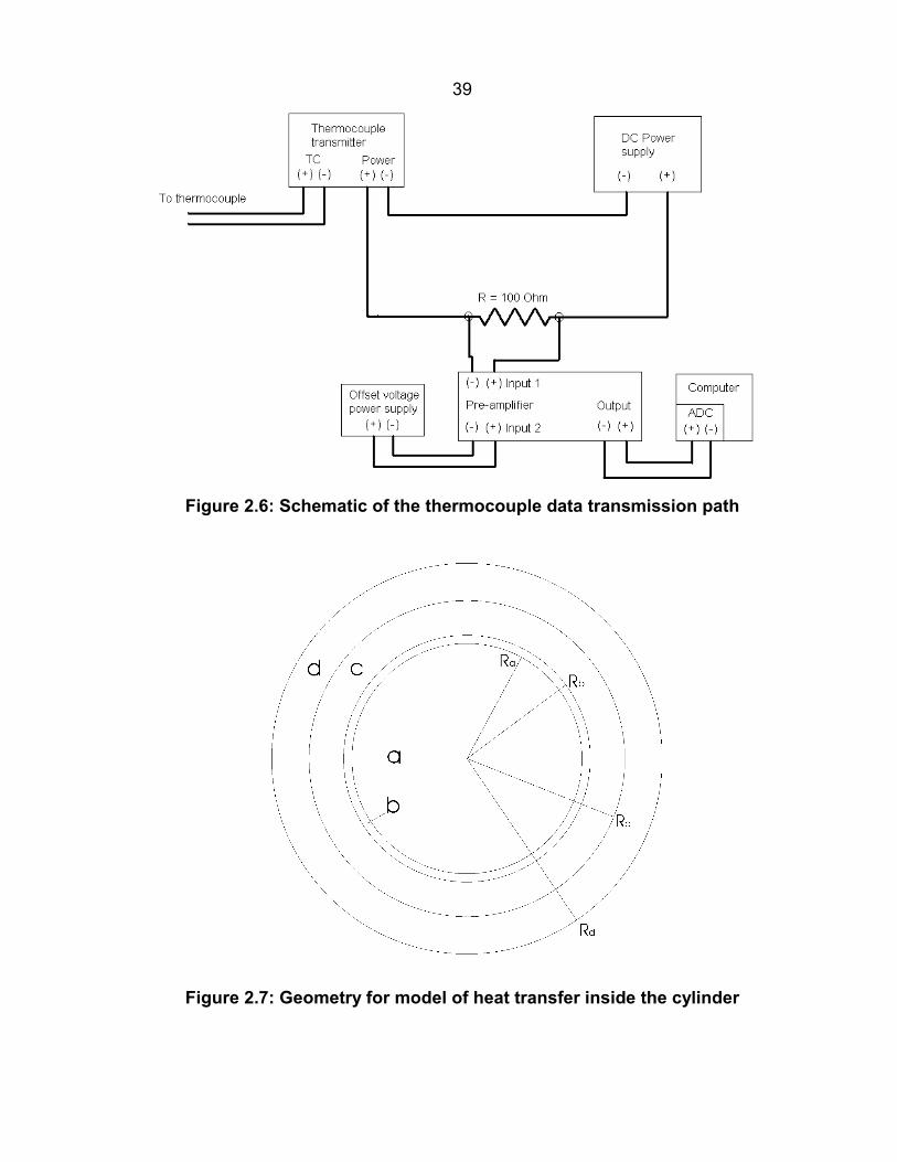
39
Figure 2.6: Schematic of the thermocouple data transmission path
Figure 2.7: Geometry for model of heat transfer inside the cylinder

40
1000
2000
3000
4000
5000
6000
1000 2000 3000 4000 5000 6000
hZhukauskas [W/m2K]
hmod
el [W
/m2 K
]D = 6.25mmD = 9.42mm
Figure 2.8: Heat transfer coefficient determined using one-dimensional modelvs. heat transfer coefficient predicted by Zhukauskas (1972) correlation

41
Figure 2.9: Illumination and imaging setup for digital particle imagethermometry/velocimetry (not to scale)

42
Figure 2.10: Color system used for TLC calibration; the white point is at theorigin, the pure RGB primaries are labeled, hue (H) is the angle between the v1axis and the color measured counterclockwise, saturation (S) is the distance
of a color from the origin, and intensity (I) is directed out of the paper; lengthsare scaled by I to make the figure applicable for any value of I

43
Figure 2.11: TLC calibration data for a sampling of color-averaging windows
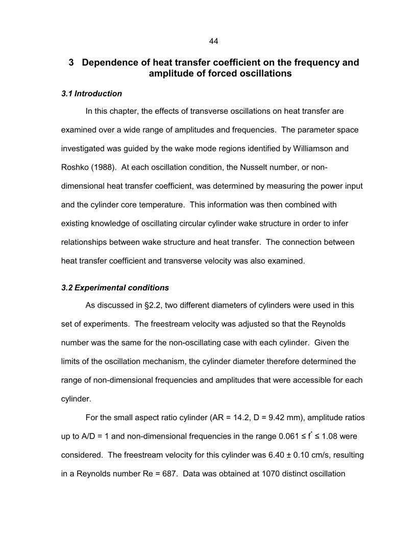
44
3 Dependence of heat transfer coefficient on the frequency andamplitude of forced oscillations
3.1 Introduction
In this chapter, the effects of transverse oscillations on heat transfer are
examined over a wide range of amplitudes and frequencies. The parameter space
investigated was guided by the wake mode regions identified by Williamson and
Roshko (1988). At each oscillation condition, the Nusselt number, or non-
dimensional heat transfer coefficient, was determined by measuring the power input
and the cylinder core temperature. This information was then combined with
existing knowledge of oscillating circular cylinder wake structure in order to infer
relationships between wake structure and heat transfer. The connection between
heat transfer coefficient and transverse velocity was also examined.
3.2 Experimental conditions
As discussed in §2.2, two different diameters of cylinders were used in this
set of experiments. The freestream velocity was adjusted so that the Reynolds
number was the same for the non-oscillating case with each cylinder. Given the
limits of the oscillation mechanism, the cylinder diameter therefore determined the
range of non-dimensional frequencies and amplitudes that were accessible for each
cylinder.
For the small aspect ratio cylinder (AR = 14.2, D = 9.42 mm), amplitude ratios
up to A/D = 1 and non-dimensional frequencies in the range 0.061 ≤ f* ≤ 1.08 were
considered. The freestream velocity for this cylinder was 6.40 ± 0.10 cm/s, resulting
in a Reynolds number Re = 687. Data was obtained at 1070 distinct oscillation

45conditions, including 64 different frequencies and 20 amplitudes, in addition to the
non-oscillating case. The specific oscillation conditions considered for this cylinder
are shown in the (1/f*, A/D)-plane in Figure 3.1.
Amplitude ratios up to A/D = 1.5 and non-dimensional frequencies in the
range 0.061 ≤ f* ≤ 0.48 were considered for the larger aspect ratio cylinder (AR =
21.3, D = 6.25 mm). A freestream velocity of 9.65 ± 0.15 cm/s was used, giving a
Reynolds number of Re = 688. A total of 765 distinct oscillation conditions—
consisting of 51 frequencies and 15 amplitudes—were investigated in addition to the
non-oscillating case. Figure 3.2 shows the specific oscillation conditions considered
for this cylinder.
For all cases with both cylinders, the input power (Pin) was 63.8 ± 0.1 W and
the freestream temperature (T∞) was 25.8 ± 0.10 °C. The power input and
freestream temperature for each case were measured to within ± 0.01 W and ± 0.02
°C. All other conditions were as described in Chapter 2.
3.3 Experimental setup and procedures
A single data acquisition run consisted of a set of amplitude-frequency
combinations to be performed for a particular cylinder. Prior to each run, the
appropriate cylinder was installed in the setup, and all electrical connections were
completed and verified. The water tunnel was then started with the pump motor
controllers set to the proper frequency to obtain the desired freestream velocity. The
freestream temperature control system was then activated, and several hours were
allowed for the water to reach the proper temperature. When the water tunnel was

46ready for the experiments, heating power was applied to the cylinder and the run
was started.
Control of the cylinder oscillations and acquisition of data was automated
using a custom LabVIEW program in order to enable the large number of cases to
be considered in a reasonable period of time. The LabVIEW program
communicated with the motion controller via an RS-232 serial connection. At the
beginning of each run, the program loaded a file containing the particular cases to
execute. For each case, there was a delay of at least 30 seconds after the cylinder
motion was started to allow the cylinder to reach its new equilibrium temperature.
Following the delay, voltage data from the embedded thermocouple was recorded
for 200 seconds at a rate of 20 samples per second. When data acquisition was
completed, the cylinder motion was stopped, and a delay of 20 seconds was
imposed before beginning the next case. This delay allowed any wake structures
generated by the cylinder motion to convect downstream a distance sufficient to
insure that they did not affect the next case.
During each run the freestream temperature, cylinder power input and
thermocouple-offset voltage were periodically monitored and recorded manually.
Following each run, these values were analyzed to make sure that the conditions
had been approximately constant. Measured variations in the conditions were
accounted for in the data processing.
Data for the small aspect ratio cylinder cases was acquired in two separate
runs. Cases with f* > 0.15 (1/f* < 6.67) were carried out in the first run, and the
remaining cases were part of a second run at a later date. All of the large aspect

47ratio cylinder cases were carried out in a single run. Within each of these runs, the
cases were in order of increasing amplitude and decreasing frequency, with the
amplitude changing more quickly.
3.4 Results
The results of these experiments are shown in Figure 3.3 and Figure 3.4.
Contours of the Nusselt number, scaled by the Nusselt number of the non-oscillating
cylinder (Nu0), are shown. The contour levels bracketing unity were selected to
indicate those values that are measurably different than one. Other contour levels
are spaced exponentially. While the contour levels are at the same values for the
two figures, the color schemes differ because the maximum contour level is at a
higher value for the large diameter cylinder data.
3.5 Discussion
3.5.1 Uncertainty and repeatability
The main sources of uncertainty in these results are the value of the constant
in the model used to determine the heat transfer coefficient, C�T, and the
measurement of the cylinder core temperature, Ttc. At the non-oscillating cylinder
heat transfer coefficient, uncertainty in C�T alone leads to an 8% to 10% uncertainty
in the heat transfer coefficient. The relative uncertainty due to C�T increases linearly
with h, so this can be a very large source of error for large heat transfer coefficients.
At the same time, the value of C�T is constant for each cylinder, so this effect is
systematic. Therefore, the magnitude of the heat transfer suffers from this source of
error, but any trends observed are not affected.
48Filtering and averaging over a large number of samples eliminates the
majority of the noise in the thermocouple signal, but the thermocouple itself is an
inherently imprecise device. The uncertainty in the measured temperature is
estimated to be ±0.1°C. Applying equation (2.6), this corresponds to a relative
uncertainty in h of 1% when h ≈ h0 and 7% when h ≈ 3h0.
The uncertainties in the other measurements used to determine h are not as
significant. The combined relative uncertainties due to length, diameter and power
input measurements are only about one sixth (1/6) of the uncertainty due to the
thermocouple for h ≈ h0. Also, the relative uncertainty due to these sources
increases with h at a slower rate than the uncertainty due to Ttc. Uncertainty in the
freestream temperature measurement contributes one tenth (1/10) as much as the
uncertainty in Ttc to the total uncertainty in h at all values of h. The additional
uncertainty introduced when non-dimensionalizing h as the Nusselt number is also
insignificant.
In addition to uncertainty, there is also systematic error in this experiment.
The uncertainty stated above for the thermocouple of ±0.1°C applies to
measurements in a single run and does not account for shifts in the data between
various runs. The data reported here is the most complete set available, but smaller
runs were carried out in the process of setting up and testing the experiment. For
the same oscillation condition carried out in different runs, the values of Nu/Nu0 were
observed to systematically shift by up to 2%. All of the trends in heat transfer
enhancement are repeatable, but the specific values of Nu/Nu0 are not. There are a
number of possible sources for this systematic shifting, including such things as drift

49in the analog-to-digital converter or change in the resistance at an electrical
connection. Since the observed shifts are generally smaller than the uncertainty in
the reported values, this does not affect the reliability of the data. However, it would
be beneficial to identify the source of the shifting in order to improve future
experiments.
3.5.2 Synchronization with the Strouhal frequency and its harmonics
For small amplitudes, heat transfer is significantly enhanced by oscillations
near the non-oscillating cylinder shedding frequency and its harmonics, as is
highlighted in Figure 3.5 and Figure 3.6. Curves of (Re/Re0)1/2 are included for
comparison to the expected increase in heat transfer if the effect of oscillations is
due only to the increase in the effective speed of the flow. At the smallest
amplitudes considered, the heat transfer coefficient is significantly enhanced near
frequencies of 1, 3 and 31 times the Strouhal frequency (recall that f*St ≈ 0.21 at this
Reynolds number) for both cylinders. For amplitude ratios greater than about 0.2,
heat transfer is also enhanced near 2 times the Strouhal frequency. These effects
persist up to amplitude ratios of about 0.4 to 0.5. For each of the heat transfer
peaks associated with Strouhal frequency harmonics f* ≥ f*St, the non-dimensional
frequency at which the peak occurs shifts toward lower frequency as the amplitude
increases. The reason for this shifting is not known.
Some aspect ratio effects are also evident in the heat transfer near Strouhal
frequency harmonics. For the smaller aspect ratio cylinder, there is an elevated heat
transfer coefficient at 32 f*St (f* ≈ 0.14). In this same non-dimensional frequency
range, the larger aspect ratio cylinder exhibits a more gradual decay away from the

50peak associated with the Strouhal frequency. In addition, the larger aspect ratio
cylinder has a lower peak associated with 3f*St for A/D = 0.3, and the peak
associated with 2f*St is not present until A/D = 0.3. The mechanism through which
aspect ratio effects the heat transfer at these conditions is not evident from this data
but will be investigated in Chapter 5.
The existence of these harmonic peaks is consistent with the work of other
authors. The range of amplitude ratios and non-dimensional frequencies in the
cases of interest is most comparable with the data of Park (1998), a sample of which
was shown in Figure 1.7. While Park does not have cases at this exact Reynolds
number, the observed trends in the data are very similar. The only significant
disagreement pertains to the low-frequency enhanced heat transfer cases. At some
Reynolds numbers and some amplitude ratios, Park found evidence of enhanced
heat transfer at 21 f*St. Park did not find any evidence of enhanced heat transfer at
31 f*St or 3
2 f*St. However, the correspondence between the 2P+2S wake mode and
the 31 f*St harmonic suggests that the present data is more consistent with observed
fluid phenomena.
3.5.3 Wake modes
Wake mode also appears to play a significant role in determining the heat
transfer coefficient. The wake mode boundaries identified by Williamson and
Roshko (1988), shown in Figure 1.2, are superimposed on the contour plots of
normalized Nusselt number in Figure 3.7 and Figure 3.8. There is clearly a
connection between wake mode boundaries and features of the contour plots. The
2S/2P boundary, near 1/f* = 5, corresponds to a region of steep gradient in the

51Nusselt number. At low frequency, there appears to be enhanced heat transfer in
the 2P+2S mode. This is more evident in the AR = 21.3 data, but it is present in the
AR = 14.2 data as well. At the highest non-dimensional frequencies observed, the
contours of Nu/Nu0 have a change in the sign of their slope for amplitude ratios
between 0.7 and 0.9. While this does not correspond exactly to a wake mode
boundary identified by Williamson and Roshko (1988), it is very near the
C(2S)/C(P+S) boundary. Given that the exact position of the wake mode boundaries
is known to vary with Reynolds number, it is likely that this slope change of the
contours is related to a wake mode boundary. In the AR = 21.3 data, there is an
unusual feature in the contours of Nu/Nu0 near 1/f* = 4, 1.1 ≤ A/D ≤ 1.4. This feature
may be related to the 2P/P+S wake mode boundary.
The features of the contour plots that have been related to wake mode
boundaries possess an additional characteristic of interest. In the heat transfer
coefficient data, the wake mode boundaries smoothly span several oscillation
conditions in the direction normal to the boundary. It might be more appropriate to
describe them as transition regions rather than boundaries. This is in contrast to
forced oscillation experiments for unheated cylinders reported in the literature. In
those experiments, the indirect indicators of wake mode—such as the phase of the
fluid forces relative to the cylinder motion—were observed to undergo abrupt
transitions between individual test conditions. The nature of the observed broad
transition regions will be examined in Chapter 4.
The apparent connection between wake mode and heat transfer coefficient
suggests that the heat transfer process is strongly dependent on how vorticity is

52distributed in the wake of the cylinder. This connection will be directly examined in
Chapter 5.
The “turbulence effect” referred to by Cheng et al. (1997) does not appear in
the current data. Rather, the region of the parameter space in which this supposed
effect was observed (1/f* < ~4, 0.314 ≤ A/D ≤ 0.628) is dominated by the third
harmonic of the Strouhal frequency and the transition from a 2S to a C(2S) wake
mode. At the time of the Cheng et al. study, these wake phenomena were not
known to affect the heat transfer, so the observed heat transfer enhancement was
attributed to an assumed new effect. The wake mode and harmonic effects
identified the current data eliminate the need for a turbulence effect to explain the
Cheng et al. (1997) data.
3.5.4 Transverse velocity
Over a significant portion of the parameter space investigated, mainly away
from Strouhal frequency harmonics and wake mode boundaries, the contours of
constant Nu/Nu0 appear to be well described by straight lines that pass through the
origin. Such lines also correspond to level curves of the cylinder’s transverse
velocity. Based upon this observation, the normalized heat transfer coefficient is
plotted versus the non-dimensional root-mean-square (rms) transverse velocity,
Vrms/U, in Figure 3.9. Since the cylinder motion is sinusoidal, the rms transverse
velocity equals 2
1 times the peak transverse velocity.
While there is significant scatter for Vrms/U less than about 1, the data
appears to partially collapse for larger values of Vrms/U. The data for the AR = 14.2
cylinder appears to follow two main curves, with a smaller number of data points

53falling between the two curves. The data for the AR = 21.3 cylinder nearly all lies on
one curve, though a small number of data points lie above that curve for Vrms/U less
than about 1.7.
It is assumed that the AR = 21.3 data lies below AR = 14.2 data due to aspect
ratio effects. If this is the only effect of aspect ratio, then there must be another
reason why the AR = 14.2 data exhibits two behaviors while the AR = 21.3 data
primarily shows only one behavior. Due to the frequency limitations of the oscillation
mechanism, higher non-dimensional frequencies were achieved for the AR = 14.2
cylinder than for the AR = 21.3 cylinder. If one branch of the smaller aspect ratio
data is limited to high values of f*, this would explain the absence of that branch from
the AR = 21.3 cylinder data. The small number of AR = 21.3 data points that lie
above the curve following the majority of the data may, in fact, be the beginning of a
second curve for that data set.
The bifurcation in the AR = 14.2 data was examined by excluding data points
associated with harmonics of the Strouhal frequency and identifying the wake mode
of each remaining data point. For purposes of understanding this bifurcation, the
wake mode boundaries are assumed to be the previously described features of the
contour plot. The results of this sorting are shown in Figure 3.10. It is apparent that
the two behaviors correspond to two different types of wake modes. Since the
C(2S) wake mode has the higher heat transfer coefficient, this explains why the AR
= 21.3 data had a few data points above the curve being followed by the majority of
data points. Only a few of the oscillation conditions considered for the higher aspect
ratio cylinder were in the C(2S) wake mode region and away from harmonic effects.

543.6 Conclusion
In this chapter, the details of an investigation into the effects of transverse
oscillations on the heat transfer from a circular cylinder over a large range of
frequencies and amplitudes were presented. Based upon the results of this
investigation, several conclusions can be drawn.
First, heat transfer is significantly enhanced by small amplitude oscillations at
frequencies near the Strouhal frequency and its harmonics. While previous authors
have observed this heat transfer enhancement, it was shown for the first time that
this effect is limited to amplitude ratios less than about 0.5.
This investigation also revealed that the wake mode is related to the heat
transfer coefficient. Many features apparent in the contour plots of normalized heat
transfer coefficient correspond to known wake mode boundaries. This relationship,
along with the enhanced heat transfer near the Strouhal frequency and its
harmonics, strongly suggests that the wake structure, i.e., the distribution of vorticity
in the wake, plays a central role in determining the heat transfer coefficient.
The transverse cylinder velocity was also shown to play a significant role in
determining the heat transfer coefficient. Previous authors have unsuccessfully
attempted to correlate the transverse velocity with the heat transfer coefficient. In
this investigation, it was shown that within a particular wake mode and away from
effects associated with the Strouhal frequency, the transverse cylinder velocity is the
primary factor responsible for variations in heat transfer coefficient.
Aspect ratio also appears to play a role in determining the level of heat
transfer enhancement that is achieved for a particular oscillation condition.
However, the basic effects and trends observed do not depend on aspect ratio.

55The largest source of error in measuring the heat transfer from a cylinder in
this experiment was found to be the construction of the cylinder itself. The most
beneficial modification to this experiment for future work would be to alter the design
of the cylinder construction so that a more reliable method for determining the heat
transfer coefficient can be developed. Such a modification might take the form of
mounting multiple temperature sensing devices flush with the cylinder surface at
various locations, thereby eliminating the need for a model to be used. It would also
be advantageous to use a more accurate and more precise type of sensor for
measuring the cylinder temperature, such as an RTD or a thermister.

56
Figures for Chapter 3
Figure 3.1: Oscillation conditions considered for the AR = 14.2 cylinder

57
Figure 3.2: Oscillation conditions considered for the AR = 21.3 cylinder

58
Figure 3.3: Contours of heat transfer coefficient normalized by non-oscillatingcylinder heat transfer coefficient (Nu/Nu0) for the AR = 14.2 cylinder

59
Figure 3.4: Contours of heat transfer coefficient normalized by non-oscillatingcylinder heat transfer coefficient (Nu/Nu0) for the AR = 21.3 cylinder

60
Figure 3.5: Normalized heat transfer coefficient (Nu/Nu0) vs. non-dimensionaloscillation frequency (f*) at selected small amplitudes for the AR = 14.2
cylinder
Figure 3.6: Normalized heat transfer coefficient (Nu/Nu0) vs. non-dimensionaloscillation frequency (f*) at selected small amplitudes for the AR = 21.3
cylinder

61
Figure 3.7: Contours of normalized heat transfer coefficient (Nu/Nu0) for theAR = 14.2 cylinder with wake mode boundaries from Williamson and Roshko
(1988) superimposed

62
Figure 3.8: Contours of normalized heat transfer coefficient (Nu/Nu0) for theAR = 21.3 cylinder with wake mode boundaries from Williamson and Roshko
(1988) superimposed

63
Figure 3.9: Normalized heat transfer coefficient (Nu/Nu0) vs. non-dimensionalrms transverse cylinder velocity (Vrms/U) for both cylinders
Figure 3.10: Normalized heat transfer coefficient (Nu/Nu0) vs. non-dimensionalrms transverse cylinder velocity (Vrms/U) for AR = 14.2 cylinder with wake
modes identified and data near harmonic synchronizations removed; curvesare least-squares polynomial fits to the data

64
4 Wake mode transitions and the mode-switching phenomenon
4.1 Introduction
In §3.5.3, the apparent existence of continuous transitions between distinct
wake modes was noted. Broad transition regions were observed to exist in the heat
transfer coefficient data, while for unheated cylinders transitions between wake
modes are abrupt, though they may exhibit hysteresis. This suggests that the
heating of the cylinder is somehow changing the wake formation process.
Identifying the nature of this change would expose part of the dynamics of wake
formation in general.
In the present chapter, these transition regions are explored in greater detail.
It will be shown that the smooth transition regions actually consist of cases where
the wake is repeatedly switching between distinct modes, a new phenomenon that is
not observed for unheated cylinders. A qualitative model describing the mechanism
for this mode-switching will be proposed. The implications of this discovery for
understanding wake modes in general will also be discussed.
4.2 Time-dependent analysis of data from earlier experiments
The analysis of data in Chapter 3, using the model described in Appendix B,
assumes that the cylinder’s heat transfer coefficient is steady. While this
assumption is in fact true for the vast majority of the cases considered, it is not
correct for all cases. Certain cases in wake mode transition regions exhibit highly
unsteady, and possibly periodic, behavior.
Figure 4.1 shows thermocouple temperature time series for 15 cases
spanning the 2S/2P transition at amplitude ratios near 0.35. The arrangement of the

65subplots corresponds to (1/f*,A/D) coordinates such that those subplots on the left
side represent cases in the 2S wake mode region, and the subplots on the right
correspond to cases in the 2P wake mode region. The 2S cases have a steady
thermocouple temperature of about 41.3°C, while the 2P cases have steady
temperatures over 43°C. The cases in the middle, however, do not have a steady
temperature. Instead, they appear to repeatedly move between the temperature
levels associated with the 2S and 2P wake modes. While the variations are not
periodic, there does appear to be a dominant timescale. For the particular cases
shown, the period of the switching is on the order of 30 to 40 seconds. The period of
switching varies from cases to case and is generally shorter for the large aspect ratio
cylinder. The timescale of these temperature variations will be examined in §4.4.
Repetition of cases indicates that the large temperature variations consistently occur
at the same conditions, and the timescales of the switching are repeatable, as well.
As noted in §3.5.3, the heat transfer coefficient, and consequently the cylinder
core temperature, depends primarily on the wake mode in this region of the
parameter space. The variation in cylinder core temperature therefore suggests that
the wake mode for these cases is in fact switching repeatedly between the 2S and
2P modes. Such a phenomenon, which will be referred to as mode-switching, has
not been observed to occur for unheated cylinders undergoing forced sinusoidal
oscillations. The only similar phenomenon is a one-time switch from the 2P mode to
the 2S mode related to startup conditions observed by Carberry et al. (2001). Later
sections of this chapter focus on determining if mode-switching is actually occurring
and on understanding the mechanism of the mode-switching.

66The smooth wake mode transitions described in §3.5.3 can now be
interpreted. The temperature used to determine the Nusselt number for each case
was the average of a 200-second time series containing 100 to 1500 cylinder
oscillations and, for cases with mode-switching, 4 to 14 cycles of mode-switching.
For cases undergoing mode-switching, the average of the time series will
correspond to some value in between the temperatures associated with the two
modes being switched between. This will lead to an apparent smooth transition
between the two modes in the heat transfer data.
It is desirable to have a single quantity that can be used to identify whether
mode-switching occurred for a particular case. The first quantity considered was the
uncertainty in the normalized heat transfer coefficient attributable to the standard
deviation in the thermocouple temperature time series
� �tctc0 T
surf
0T
2
tc
0NuNu TT
NuNuTNuNu
��
�����
����
��
�
. (4.1)
This did not perform well for identifying mode-switching because it is too heavily
weighted by the heat transfer coefficient. The direct dependence on the heat
transfer coefficient was therefore removed to form a normalized quantity
��
�
�
�
TTNuNu surf
T
0
NuNu tc0 , (4.2)
which performed significantly better. Contours of this normalized standard deviation
are plotted in Figure 4.2 and Figure 4.3.
It is evident that mode-switching is confined to particular areas of the
(1/f*,A/D) plane. In Figure 4.4 and Figure 4.5, the Williamson and Roshko (1988)
wake mode boundaries are superimposed on the standard deviation contours.

67Mode-switching is particularly strong along the 2S/2P boundary, and it is also
significant along the C(2S)/C(P+S) boundary. There is also evidence that mode-
switching occurs in the region where the 2P, P+S and C(P+S) modes come
together. However, mode-switching does not occur at all wake mode boundaries.
Switching also occurs around the harmonics of the Strouhal frequency. In
these cases, the switching is not between distinct modes, but rather between wake
structures that are synchronized with the harmonic frequency and structures that are
not synchronized with the harmonic.
The regions of mode-switching occur at the same non-dimensional conditions
for both of the cylinders used in this study. These conditions correspond to
significantly different dimensional frequencies and amplitudes, which indicates that
the mode-switching is a real fluid mechanical phenomenon related to the wake
structure, not a spurious noise signal.
4.3 Verification of wake mode-switching
In order to verify that the presumed switching between wake modes is taking
place, DPIV and thermocouple data were acquired simultaneously for an oscillation
condition known to exhibit the signs of wake mode-switching. The condition 1/f* =
5.60, A/D = 0.35 was chosen because it had the highest value of � �0Nu/Nu Nu/Nu0
�
observed in the initial parameter space survey. This condition lies in the 2S/2P
transition region.
DPIV data was acquired using the same setup as used for DPIT/V (described
in §2.7), but the color content was not calibrated so no temperature information was
obtained. Synchronization of the images with the thermocouple data was

68accomplished by recording the light sheet timing signal along with the thermocouple
data. In order to resolve the timing signal, both signals were sampled at 500
samples per second. The DPIV data rate corresponded to 12.4 image pairs per
cycle.
Figure 4.6 shows the recorded thermocouple signal as a function of time. If
the hypothesis that the temperature fluctuations are caused by changes in wake
mode is correct, there should a 2S wake mode when 0dtdTtc � , and there should
be a 2P wake mode when 0dtdTtc � . The portions of Figure 4.6 that are marked
with heavy lines are the times chosen to examine the wake mode. The times when
the temperature was near its minimum and maximum values were not included
because of a possible time lag between the actual mode-switching and the
temperature signal.
The DPIV data corresponding to the indicated times was divided into two
groups by the sign of the temperature slope. The negative slope group contained
31.5 cycles of the cylinder motion, and the positive slope group contained 19.4
cycles. The vorticity fields for each group were phase averaged with respect to the
motion of the cylinder. The cylinder motion was divided into 16 equally sized phase
“bins,” and all of the flow snapshots in a bin were averaged together.
The resulting phase averaged vorticity fields are shown in Figure 4.7 and
Figure 4.8. Eight of the 16 phases of the cylinder motion are shown, with every
other phase being omitted. As predicted, the negative temperature slope vorticity
fields exhibit a 2S wake mode, while the positive temperature slope vorticity fields
show a 2P wake mode. This confirms that wake mode-switching is taking place.

694.4 Connection between temperature and wake mode
In order to determine the mechanism behind the observed mode-switching,
the timescale of the switching was compared to a number of possible sources.
Table 4.1 lists several known timescales in the flow. None of these timescales is on
the same order as the observed timescale of the mode-switching. There is also no
apparent correlation between the oscillation frequency and the mode-switching
frequency.
There is one additional timescale present in the experiment due to the
manner in which the cylinder is heated. As described in §2.3 and §2.6, the power
input to the cylinder is held constant and the heat transfer coefficient then
determines the resulting cylinder core temperature. If the heat transfer coefficient of
the cylinder changes, there will be some amount of time required before the cylinder
core reaches its new equilibrium temperature. It is possible that this cylinder thermal
timescale is related to the mode-switching. However, the cylinder thermal timescale
is not known and must be modeled.
In designing this set of experiments, it was assumed that the cylinder’s heat
transfer coefficient for a particular oscillation condition was steady. If this were the
case, the only effect of the cylinder thermal timescale would be on the length of time
required for the system to reach steady state. A rough estimate of the cylinder time
scale was considered sufficient to estimate the necessary delay to allow the
transient behavior to pass before recording data. In the unsteady cases, it is
desirable to know the thermal time scale more accurately.
In order to determine the cylinder thermal time constant, a time-varying
version of the internal heat transfer model was developed. It was constructed to

70simulate the cylinder’s thermal response to a step change in the heat transfer
coefficient at t = 0. The details of the unsteady model derivation can be found in
Appendix C. The time constant for each cylinder was found to depend only on hf,
the heat transfer coefficient for t ≥ 0. The calculated thermal time constants for
various Nusselt numbers are shown in Figure 4.9. These time constants are of the
same order as the observed mode-switching timescales. Variations in the observed
timescale follow the trend of the model values, with shorter timescales
corresponding to higher heat transfer coefficients.
This agreement between the timescale of mode-switching and the thermal
time constant of the cylinder suggests that the observed temperature fluctuations are
setting the period of the wake mode-switching. This implies that some type of
feedback loop exists between the wake mode and the cylinder temperature. Of
particular significance, this means that temperature is not a passive scalar in this
flow.
A simulation was carried out using a simple hysteresis model in order to verify
that a coupling between temperature and wake mode can produce the observed
variations in cylinder core temperature. In the model, once the cylinder oscillations
begin, the heat transfer coefficient can take on two possible values, h1 or h2. The
heat transfer coefficient is determined by the cylinder surface temperature and the
current state of the heat transfer coefficient as shown by the hysteresis loop in
Figure 4.10. This model makes no attempt to identify the specific mechanism by
which temperature affects the wake mode. The unsteady model of internal heat
71transfer developed in Appendix B was modified to allow hf to take on the proper
value according to this hysteresis loop.
Figure 4.11 shows the resulting temperature history on the cylinder using an
initial condition corresponding to the stationary cylinder, h1 equaling a typical value
for the 2S mode, h2 having a value typical of the 2P mode, and the properties of the
AR = 14.2 cylinder. The switching temperatures, T1 andT2, were chosen to give
approximately the observed variation in cylinder core temperature. While this model
results in a periodic solution after the first mode-switch and not the quasi-periodic
behavior observed in the experiments, the general features agree quite well. The
timescale for the mode-switching is off by a factor of only 1.5. It is not surprising that
such a simple model, which ignores all of the physics of the mode-switching
mechanism, does not agree with the experiments in every detail. In fact, the high
degree of similarity to the experimental results indicates that an abrupt change in the
heat transfer coefficient induced by a change in surface temperature is a fairly good
model of the mode-switching phenomenon.
4.5 Mode-switching mechanism model
The timescale of the observed mode-switching indicates that the cylinder
temperature affects the cylinder wake structure but does not reveal the mechanism
by which the temperature acts. That mechanism must be inferred indirectly.
Temperature induced changes in the kinematic viscosity in a portion of the attached
boundary layer are believed to be the means by which the temperature affects the
wake structure.

72Any plausible mechanism for mode-switching must allow for an incompatibility
between the cylinder wake mode and the surface temperature it leads to. In
addition, this incompatibility must drive the system towards a change in wake mode
for some conditions. More specifically, it is necessary that in the mode-switching
cases, the steady-state cylinder surface temperature corresponding to a particular
wake mode causes the wake to switch out of that mode and in to a different mode.
Such an incompatibility between wake structure and cylinder temperature may not
always lead to mode-switching. For example, in the 2P mode the magnitude of the
circulation of the leading and trailing vortices in a pair can be nearly equal or vastly
different. Also, in Chapter 3 it was shown that the heat transfer coefficient varies
more gradually within a wake mode than across mode boundaries. If the distribution
of vorticity in the wake can adjust to the cylinder temperature sufficiently to reach
either a limit cycle or equilibrium without changing wake mode, then no mode-
switching will occur and no large fluctuations will appear in the temperature time
series. Mode-switching is only observed to occur at particular oscillation conditions,
so in the majority of cases the mechanism must lead the wake structure and the
temperature to converge to either an equilibrium state or to a limit cycle entirely
within one mode.
Temperature does not explicitly appear in the equations of motion describing
this flow. However, temperature does enter indirectly through material properties.
Of particular importance are density and viscosity. Temperature induced density
differences will result in buoyancy forces on the fluid. Care was taken in designing
the experiments to make sure that these buoyancy forces are not significant

73compared to inertial forces, so this is not considered as a possible mechanism.
Viscosity differences, on the other hand, may be significant. While the density
changes by only 0.3%, the kinematic viscosity of fluid at the cylinder surface is up to
20% lower than in the freestream. This can have a substantial effect on the flow
near the cylinder. Therefore, temperature induced variations in the viscosity are
thought to be the connection between wake mode and temperature.
Figure 4.12 shows the proposed model to explain the observed wake mode-
switching phenomenon. The cylinder surface temperature sets the temperature
profile of the thermal boundary layer, which then determines the viscosity in that
layer. This will have an effect on the boundary layer velocity profile, which is also a
function of the outer flow and of the existing wake. The influence of the existing
wake allows hysteresis to enter the model. The boundary layer velocity profile and
the outer flow determine the flux of vorticity and kinetic energy into the free shear
layers. Following the ideas of Jeon and Gharib (2003), the kinetic energy of the fluid
elements carrying the vorticity flux into the wake determines when a vortex pinches-
off from the free shear layers, thereby determining the resulting wake mode. The
cylinder surface temperature, therefore, is one factor that controls the distribution of
vorticity in the wake, or the wake mode. As was demonstrated in §3.5.3, the wake
mode is one of the factors that determine the cylinder heat transfer coefficient, which
will set the surface temperature if the power input is constant. The loop is closed,
and it is possible for feedback between the temperature and the wake structure to
exist.

74This mechanism is not equivalent to fluctuations in Reynolds number caused
by temperature variations, though there is some similarity. The effect of varying
cylinder temperature is not the same as if the freestream temperature is changed
becasue the temperature is not uniform across the thermal boundary layer, and the
thermal boundary layer is much thinner than the velocity boundary layer at the
Prandtl number in this experiment. However, an analogy to a Reynolds number
effect is useful. As mentioned in §1.2.1, the locations of wake mode boundaries
depend on the Reynolds number and exhibit hysteresis. For a fixed oscillation
frequency and amplitude, a change in Reynolds number due to a change in the fluid
viscosity may, under the proper conditions, cause a wake mode boundary to move
past the oscillation state. Due to hysteresis, there would be a finite difference in the
Reynolds number at which switching occurs depending on the current wake mode.
This would require a time delay and a temperature difference between successive
mode-switches.
One significant implication of this model for the mechanism is that the sign of
the derivative of kinematic viscosity with respect to temperature, d�/dT, is critical in
determining if mode-switching occurs. This is related to the requirements for a
plausible mechanism previously described. Had these experiments been conducted
in air or in another fluid for which kinematic viscosity increases with increasing
temperature, the conditions in this set of experiments that resulted in mode-
switching would have presumably driven the wake mode boundary away from the
oscillation state instead of towards it. The Prandtl number and its derivative may
also play a role in determining the conditions for which mode switching occurs.

75This proposed mechanism also implies that the heat transfer coefficient
produced by a particular oscillation condition will depend on the cylinder input power
or temperature. This is one possible way to test the model. Another way to test the
model would be to perform detailed numerical simulations of the flow and heat
transfer including explicit dependence of viscosity on temperature.
4.6 Conclusion
A new phenomenon was discovered in which the wake structure repeatedly
switches between distinct wake modes or between variations of a single wake mode.
The mechanism of this mode-switching is believed to be temperature induced
variations in the fluid viscosity resulting in changes to the flux of vorticity and kinetic
energy into the wake.
By highlighting the possible role of viscosity and of the separated shear layer
fluxes in the determination of wake mode, this discovery may lead to improved
understanding of the vortex formation and pinch-off processes in wakes in general,
not just in heat transfer applications.
Additional investigations into mode-switching are necessary. Determining
criteria for the occurrence of mode-switching would reveal a great deal about wake
formation processes in general. This requires that the proposed model of the mode-
switching mechanism be tested and made quantitative. To this end, numerical
simulations in which the temperature dependence of viscosity can be prescribed or
eliminated would be useful.

76
Tables and figures for Chapter 4
Table 4.1: Known timescales present in the flow
Source / phenomenon Timescale (sec)Cylinder oscillations 0.14 – 2.2Water tunnel pumps 0.13 – 0.20
Water tunnel sloshing ~3Water tunnel recirculation ~120
0 100 20041
42
43
44
A/D
= 0
.400
1/f* = 5.31
0 100 20041
42
43
441/f* = 5.45
0 100 20041
42
43
441/f* = 5.60
0 100 20041
42
43
441/f* = 5.75
0 100 20041
42
43
441/f* = 5.89
0 100 20041
42
43
44
A/D
= 0
.350
0 100 20041
42
43
44
0 100 20041
42
43
44
0 100 20041
42
43
44
0 100 20041
42
43
44
0 100 20041
42
43
44
time (sec)
A/D
= 0
.300
0 100 20041
42
43
44
time (sec)0 100 200
41
42
43
44
time (sec)0 100 200
41
42
43
44
time (sec)0 100 200
41
42
43
44
time (sec)
Figure 4.1: Time series of thermocouple temperature for several oscillationconditions near the 2S/2P transition using the AR = 14.2 cylinder

77
Figure 4.2: Contours of normalized standard deviation of heat transfercoefficient time series ( � �0Nu/Nu Nu/Nu
0� ) for the AR = 14.2 cylinder

78
Figure 4.3: Contours of normalized standard deviation of heat transfercoefficient time series ( � �0Nu/Nu Nu/Nu
0� ) for the AR = 21.3 cylinder

79
Figure 4.4: Contours of normalized standard deviation of heat transfercoefficient time series ( � �0Nu/Nu Nu/Nu
0� ) for the AR = 14.2 cylinder with wake
mode boundaries from Williamson and Roshko (1988) superimposed

80
Figure 4.5: Contours of normalized standard deviation of heat transfercoefficient time series ( � �0Nu/Nu Nu/Nu
0� ) for the AR = 21.3 cylinder with wake
mode boundaries from Williamson and Roshko (1988) superimposed

81
Figure 4.6: Time series of thermocouple temperature for data set synchronizedwith DPIV using AR = 14.2 cylinder oscillating at 1/f* = 5.60, A/D = 0.35; times
represented by heavy lines are included in the phase averaged DPIV data

82
Figure 4.7: Phase averaged non-dimensional vorticity ( UD� ) for 0dtdTtc � ;cylinder motion divided into 16 phase bins, every other bin shown; positive
vorticity contours are solid, negative vorticity contours are dashed; minimumcontour levels = ± 0.33, contour spacing = 0.33
Figure 4.8: Phase averaged non-dimensional vorticity ( UD� ) for 0dtdTtc � ;cylinder motion divided into 16 phase bins, every other bin shown; positive
vorticity contours are solid, negative vorticity contours are dashed; minimumcontour levels = ± 0.33, contour spacing = 0.33

83
Figure 4.9: Cylinder thermal time constant (�) as a function of normalized heattransfer coefficient (Nu/Nu0)

84
Figure 4.10: Hysteresis loop used to in simulation to represent the unknownmode-switching mechanism
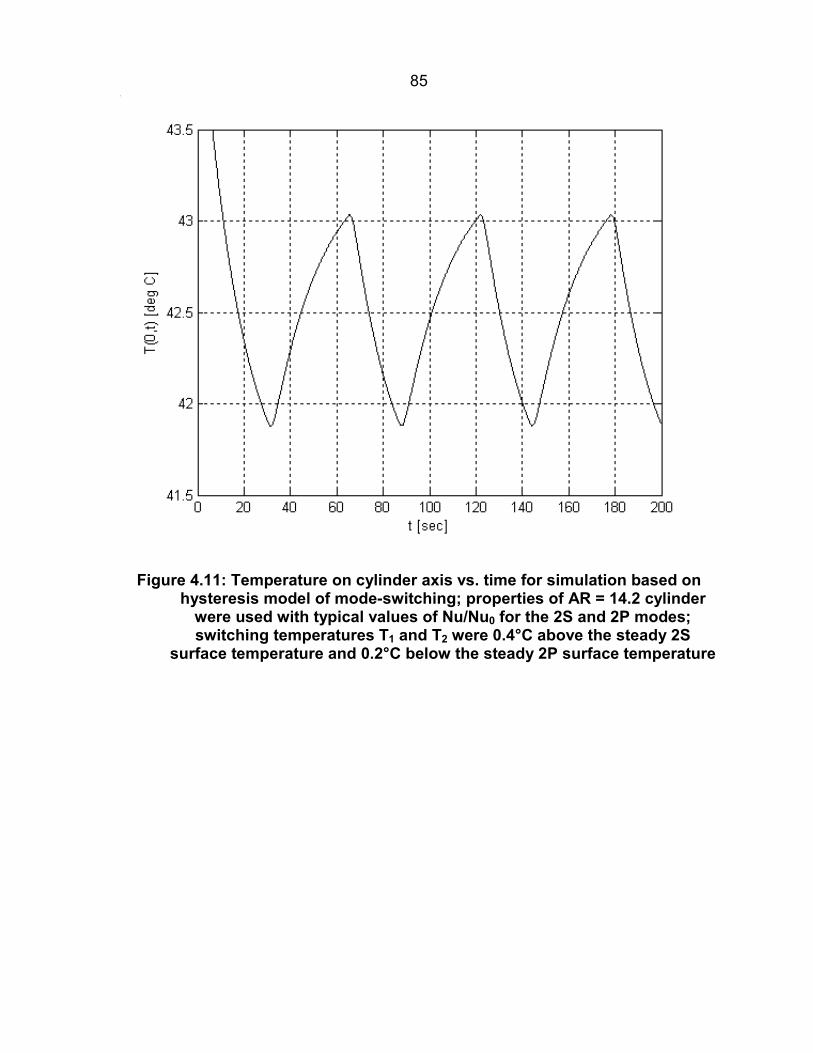
85
Figure 4.11: Temperature on cylinder axis vs. time for simulation based onhysteresis model of mode-switching; properties of AR = 14.2 cylinder
were used with typical values of Nu/Nu0 for the 2S and 2P modes;switching temperatures T1 and T2 were 0.4°C above the steady 2S
surface temperature and 0.2°C below the steady 2P surface temperature

86
Figure 4.12: Model of the mode-switching mechanism
87
5 Wake structure and convective heat transfer coefficient
5.1 Introduction
In this chapter, results of experiments using DPIT/V to measure the
temperature and velocity fields in the wake of heated oscillating cylinders are
presented. These experiments were conducted in order to determine how wake
structure affects heat transfer. Several new mechanisms were revealed, including
the vortex dynamics during roll-up and the spacing between shed vortices. The
effects of transverse cylinder velocity and cylinder aspect ratio were also identified.
5.2 Experimental conditions
A total of 44 different cases were investigated in the DPIT/V experiments on
wake structure. This includes two non-oscillating cases and several cases that
overlap in oscillation amplitude and frequency, though not in aspect ratio. The
specific cases chosen are indicated in Figure 5.1 and in Table 5.1 and Table 5.2.
The two different symbols in the figure indicate the two different aspect ratios of
cylinders that were used in the experiments. The non-oscillating cases are shown in
Figure 5.1 for reference at the natural shedding frequency and zero amplitude.
The cases were chosen to be representative of the full range of wake
structures accessible with the experimental setup. Experiments were conducted in
each wake mode region and at all of the Strouhal frequency harmonics evident in
the data presented in Chapter 3. It was necessary to use the low aspect ratio
cylinder to access high non-dimensional frequencies and to use the higher aspect
ratio cylinder to achieve large amplitude ratios. Both cylinders were used in the
88areas where significant discrepancy between the two data sets existed,
corresponding to the 31 and 3
2 sub-harmonics of the Strouhal frequency.
In several areas of the parameter space, clusters of cases were investigated.
This allowed unusual features of Figure 3.3 and Figure 3.4—such as near 1/f* ≈ 4,
A/D ≈ 1.1—to be studied more closely. Clusters of cases were also used to
investigate the role of transverse velocity in determining the heat transfer coefficient
within a wake mode.
In order to distinguish between cases, each case was assigned a letter and
number. The letter S indicates the smaller aspect ratio (or short) cylinder, and L
indicates the larger aspect ratio (or long) cylinder. For both cylinders, case 0 is the
non-oscillating case. All oscillating cases are numbered in order of decreasing
frequency, i.e, from left to right in Figure 5.1, for that cylinder. For cases with the
same frequency, the smaller amplitude case has the lower number. The numbers
corresponding to each oscillation condition are shown in Figure 5.2 and Figure 5.3.
5.3 Experimental setup and procedures
These experiments were carried out using the experimental setup described
in Chapter 2. The details of the DPIT/V setup are located in §2.7, along with many
of the procedures for acquiring and processing the data.
Data was acquired for this set of experiments in two separate runs, one for
each of the two different aspect ratio cylinders used. Each run consisted of
preparing the water tunnel, acquiring simultaneous DPIT/V and thermocouple data
for each of the cases, and acquiring DPIT calibration data.

89In order to obtain the best possible temperature data, it was necessary to
thoroughly clean and properly prepare the water tunnel before the experiments. The
cleaning was necessary to remove TLC particles that were used in the tunnel
previously because they have a different color-temperature relationship than the
newly added particles. The day prior to a run, the water tunnel was drained and all
of the accessible surfaces were cleaned with a soft brush. Next, the honeycomb
and screens were removed from the upstream section and cleaned using a brush
and mild soap, then rinsed thoroughly. The tunnel was refilled with filtered water,
run at high speed to stir up any loose particles, then drained again. Finally, the
tunnel was filled with filtered water, the honeycomb and screens were replaced, and
the filter and temperature control loop were left running overnight.
Before being added to the water tunnel, the TLC particles were heated past
their blue clearing temperature. The calibration curve of the TLC can shift after the
particles are exposed to temperatures above the blue clearing point. If this were to
happen during the experiment, the calibration would be incorrect. Therefore, the
particles were pre-heated so that any shift took place before the experiments began.
Approximately 40 mL of TLC slurry was diluted in 1000 mL of de-ionized water. The
particles were then heated and mixed using a hot plate/stirrer until the blue clearing
temperature was exceeded. This process took about 25 minutes.
The TLC particles were then added to the water tunnel through a sieve with
75 �m openings. This removed any large particles or clumps of particles that would
either fail to follow the flow or produce over-saturated images. The resulting particle
loading of the tunnel was about 0.02% by volume. Approximately 30 minutes, or 15

90tunnel re-circulation times, was allowed for the TLC particles to mix with the water in
the tunnel. This time also allowed for an equilibrium amount of water to penetrate
the protein encapsulation of the TLC particles.
Acquisition of DPIT/V and thermocouple data was automated to allow the set
of cases to be investigated in a period of time over which the TLC color-temperature
relationship remains fairly constant. The basic program was a modified version of
the LabVIEW program described in §3.3. Additional code was added so that the
program triggered the light sheet pulsing and the acquisition of video images. This
resulted in synchronized DPIT/V and thermocouple data for each case. The number
of cylinder oscillation cycles recorded for each case are listed in Table 5.1 and Table
5.2.
After data was acquired for each case in the run, DPIT calibration data was
acquired. First, the water tunnel temperature control loop was set to a temperature
just below the red clearing temperature for the TLC particles. As the water was
cooling down, the cylinder was removed from the tunnel, and the RTD probe for the
reference thermometer was moved to a location in the contraction immediately
upstream of the test section. The procedure for acquiring calibration images
described in §2.7 was then followed.
During the acquisition of data and calibration images, the water tunnel
temperature was monitored using a reference thermometer. Between the two runs
of data acquisition for this part of the study, the original reference thermometer
(Fluke 2180A) stopped working properly. A new reference thermometer (Omega
DP41-RTD) was therefore used for the large aspect ratio cases. There is fixed

91offset between the two thermometers of 0.2°C, though temperature differences were
measure to a precision of 0.02°C for each. All temperatures measured with the new
thermometer were referenced back to the original thermometer.
However, the offset was initially misidentified, and this resulted in the large
aspect ratio cases being run with a freestream temperature of 25.4°C instead of
25.8°C. This does not significantly affect the Reynolds number and was accounted
for in the computation of Nusselt number. The major effect of this is that the large
aspect ratio cases were run at a freestream temperature where the relationship
between temperature and hue for the TLC particles is not monotonic. This means
that a portion of the range of the TLC is lost, and only the highest temperatures are
reliably known. Therefore, the temperature data for these 14 cases was
disregarded. Temperature data will only be considered for the 31 small aspect ratio
cases.
After processing each pair of data images for a particular case, averaging of
the data was performed. Several types of averaging were used: phase-averaging,
balanced full-cycle averaging, and unbalanced averaging of the full data set. For
phase-averaging, snapshots of the flow were grouped by the phase of the cylinder
motion and the mean and rms of the groups were computed as
2b
n
2bn
bn
2bn
brms,b
bbnbn
nbn
bb
qqN1q
N1q
qqq
qN1q
���
��
�
��
�
�
� . (5.1)
In these definitions, q is some property of the flow such as a velocity component, the
temperature or the vorticity, b is the index indicating the phase bin, Nb is the number

92of snapshots in bin b, and n is the index of snapshots in bin b. In some cases,
where the flow was expected to vary on a time scale of several oscillation cycles, the
phase groupings extended over that number of oscillation cycles.
The balanced full-cycle averaging was intended to represent the overall mean
and rms of the flow with each phase of the oscillation cycle equally represented.
The balanced average and rms were therefore defined as
� ��
�
���
�
b
2mean
2b
2rms,brms
bbmean
qqqB1q
qB1q
, (5.2)
where B is the number of phase bins. This form of averaging was used for all of the
oscillating cases.
For the non-oscillating cases, there is no oscillation phase with which to
synchronize. It is possible to define a phase based on the velocity fluctuations in the
wake, as was done by Park (1998). However, this was not found to aid in
interpreting the data. For these cases, the individual snapshots were all averaged
together to determine the mean and rms values
2mean
n
2n
n
2nrms
meannn
nnmean
qqN1q
N1q
qqq
qN1q
����
���
�
��
�
. (5.3)
Here, N is the total number of snapshots.
For phase-averaged quantities, values are presented in lab coordinates, so
the cylinder is fixed in the x direction and moves in the y direction. When
considering the mean flow, all quantities are presented in a coordinate system fixed

93with respect to the cylinder. This is so that it is evident how features of the flow
would affect the heat transfer from the cylinder.
5.4 Results
A typical pair of data images, taken from case S19, is shown in Figure 5.4.
The instantaneous normalized velocity, vorticity and temperature fields
corresponding to this image pair are shown in Figure 5.5, Figure 5.6 and Figure 5.7.
The gray rectangle in the velocity and vorticity plots indicates data that is not reliable
because of the cylinder’s image and shadow. In the plot of the temperature field, the
dotted line indicates the streamwise location upstream of which the temperature
range of the TLC particles was not sufficiently large to be useful.
Certain results are summarized for each case in Table 5.1 and Table 5.2,
including the normalized Nusselt number, its standard deviation and the observed
wake mode. The wake mode abbreviations are mainly taken from Williamson and
Roshko (1988). The abbreviation NS indicates that no synchronization with the
cylinder motion was observed. Two modes separated by a forward slash, /,
indicates that mode-switching between those two modes was observed. Other
abbreviations follow the scheme of Williamson and Roshko, with number-letter
combinations indicating the number of single vortices or pairs of vortices shed per
cycle.
Beginning with Figure 5.8 and continuing through Figure 5.141, various plots
for each case are presented. For all cases, the mean and rms velocity and vorticity
fields are presented. For the oscillating cases, the phase-averaged vorticity fields

94are also included. For the small aspect ratio cases, the phase-averaged
temperature fields are also shown.
5.5 Discussion
5.5.1 Uncertainty
Before beginning a detailed discussion of uncertainty, a comment must be
made about the temperature field. For cases S1 through about S20, the measured
temperature is aberrantly high in the middle-bottom region of every snapshot. This
effect becomes smaller for each case in this range. This is believed to be caused by
a shift in the TLC color-temperature relationship over the course of the experiment.
It is not clear why the effect is limited to this region. Because the calibration was
carried out at the end of the run, the temperatures in this region for the later cases
are accurate, while the earlier cases are inaccurate. This suggests that shorter runs,
consisting of fewer cases, should be used in future DPIT/V studies.
The temperatures measured using DPIT/V in this experiment are limited to a
resolution of about ±0.1°C. For most of the cases examined in this experiment, this
resolution is sufficient to observe the significant temperature variations in the
cylinder wake. However, for cases with very high heat transfer coefficients, the
actual temperature differences are much smaller than this. At the highest heat
transfer coefficients seen in this experiment, the cylinder surface temperature is only
0.7°C hotter than the freestream fluid. In addition, over the entire range of heat
transfer coefficients observed, the temperatures in the wake are closer to the
freestream temperature than to the cylinder surface temperature—typical maximum
values of (T-T∞)/(Tsurf- T∞) are around 0.5. It is therefore beyond the capabilities of

95the present implementation of DPIT/V to measure the temperature field in the wake
of certain cases with very high heat transfer coefficients. Data was still taken for
these cases so that the velocity field could be measured. Cases S2, S3, S4 and S6
(Figure 5.14, Figure 5.17, Figure 5.20 and Figure 5.30) yield no useful temperature
field information. Some information can be extracted from cases S10 and S13
(Figure 5.50 and Figure 5.63), but the signal to noise ratio is low.
5.5.2 Identifying wake mode
The wake mode for each case was identified in order to compare with the
wake mode boundaries identified by Williamson and Roshko (1988) and the features
of Figure 3.3 and Figure 3.4. The observed modes are tabulated in Table 5.1 and
Table 5.2. For most cases, the mode is easily identifiable from the phase-averaged
vorticity plots. However, the modes for some cases are more difficult to identify.
For cases S2, S3, S4 and S6 (Figure 5.12 to Figure 5.20, and Figure 5.28 to
Figure 5.30) the wake mode is not obvious. The contours of vorticity are very
irregular, and the temperature field cannot be resolved (see §5.5.1). The best
indicators of mode in these cases are in fact the mean velocity and vorticity fields.
The mean velocity field is essentially symmetric about the x-axis, and the vorticity
field is anti-symmetric. Therefore, the wake mode must be a symmetric mode. The
specific mode was identified as C(2S) by comparing the mean and phase-averaged
fields to the C(P+S) cases S10, L1, L2 and L3 (Figure 5.48 to Figure 5.50 and Figure
5.116 to Figure 5.121). The similarity of the plots to the single vortex side of the
asymmetric mode indicated the nature of the mode for these cases.
96For case S28 (Figure 5.106 to Figure 5.108), it is also not clear how to identify
the mode. The phase-averaged vorticity plots are distinct, and the motion of
individual vortices can be followed, indicating that the shedding is synchronized with
the cylinder motion. On the other hand, the first two single vortices shed are much
larger than the third and fourth. The mode is clearly not symmetric with respect to
the cylinder motion, but it is in some way synchronized. It is not clear if this should
be considered non-synchronized or 4S (four single vortices per cycle).
In general, the wake modes agree well with the modes expected based upon
the Williamson and Roshko boundaries and the features of Figure 3.3 and Figure
3.4. The only significant exceptions are for several of the low frequency cases.
Cases S25, S27, S29, and possibly S28 (Figure 5.97 to Figure 5.99 and Figure
5.103 to Figure 5.111), all exhibit wake structures that are synchronized with the
flow. According to the Williamson and Roshko boundaries, these cases should all
be non-synchronized. It is possible that the disagreement is due to DPIV being a
more sensitive technique than the floating particle traces used by Williamson and
Roshko. For cases L12 and L13 (Figure 5.138 to Figure 5.141), though the wake is
synchronized with the cylinder motion, there does not appear to be significant pairing
between opposite signed vortices. The wakes for these cases appear to be
essentially Kármán Vortex Streets, with the shedding locked onto 3 times the
oscillation frequency. For this reason, these cases are labeled as 6S, not 2P+2S.
5.5.3 Formation length
Park (1998) suggested that the vortex formation length, �f, significantly affects
the heat transfer coefficient. The vortex formation length in turn depends on the

97oscillation conditions. According to Park, for highly synchronized cases the wake
vortices form close to the cylinder base and are therefore effective at removing hot
fluid from the base region. For cases that are not strongly synchronized, the vortex
roll-up process occurs far downstream of the cylinder, and the resulting heat transfer
is near that of the non-oscillating cylinder. The formation length can also be long for
some synchronized cases, such as cases L12 and L13 (Figure 5.138 to Figure
5.141) near the 1/3 sub-harmonic of the Strouhal frequency.
In order to compare with Park’s results, the formation length was determined
for all cases in which the wake consists only of single vortices, not pairs. This
restriction is necessary because of the methods by which the formation length was
determined. The formation length was determined in two different ways.
The first method is that used by Park. Park defined the formation length as
the distance from the cylinder to the end of the wake bubble, or closed wake, in the
mean velocity field. This location was identified using the critical point analysis of
Perry and Fairlie (1974). For two-dimensional, incompressible flow only one of the
invariants used by Perry and Fairlie, defined for the mean velocity field as
� �meanudetQ �� , (5.4)
can take on a non-zero value. This quantity can be defined at each point in the flow
where velocity data exists. If Q > 0 at a particular point, fluid at that point is
undergoing rotation and is in the neighborhood of a center. Values of Q < 0 indicate
that the point is in a saddle region. For this experiment, the quantity Q was
computed at each point for which velocity data existed along a line located slightly
off (y/D = -0.14 for AR = 14.2 and y/D = 0.08 for AR = 21.3) of the mean centerline of

98the cylinder. Along this line, fluid inside the wake bubble is in the neighborhood of a
center so Q > 0, while the end of the wake bubble is a saddle region where Q < 0.
The formation length was therefore taken to be the streamwise distance from the
cylinder base to the first point on this line with a value of Q < 0.The second method
used to determine the formation length was based upon the rms vorticity field. The
formation length was defined as the streamwise distance from the cylinder base to
the location of the peak rms vorticity on the same line. While these definitions for
the formation length generally agree with each other for wakes consisting of only
single vortices, they do not perform well for wakes with paired vortices.
Normalized heat transfer coefficients are plotted versus formation length in
Figure 5.142. The horizontal error bars in Figure 5.142 correspond to the DPIV grid
spacing, and the vertical error bars are due to the uncertainty in the measured heat
transfer coefficient.
The present data supports Park’s conclusion that short formation length
corresponds to enhanced heat transfer. The large number of cases in the present
study clarifies the relationship between formation length and heat transfer. While
Park’s data was consistent with a linear relationship between these two factors, the
present data indicates that some type of threshold effect occurs. For �f > ~1.5, there
is no significant change in Nu/Nu0 for different formation lengths. For �f < ~1.5,
there is significant heat transfer enhancement, but the value of Nu/Nu0 varies widely
over a small range of formation lengths. This suggests that formation length is not
the only factor that determines the heat transfer coefficient. It appears that a short

99formation length is necessary for significant heat transfer enhancement, but the
magnitude of the enhancement is determined by other details of the wake structure.
5.5.4 Streamwise spacing between vortices
A comparison of cases S14, S17 and S20 (Figure 5.64 to Figure 5.66, Figure
5.73 to Figure 5.75 and Figure 5.82 to Figure 5.84) reveals that the spacing between
shed vortices plays a role in determining the heat transfer for 2S mode cases. The
vortex spacing is a function of the vortex convective speed and the vortex shedding
frequency, which in synchronized cases is equal to the oscillation frequency. While
the formation process of the vortices prior to pinch-off appears almost identical for
these three cases, the spacing of the shed vortices differ considerably. In these
three cases, larger vortex spacing corresponds to higher heat transfer enhancement.
The reason for this correspondence is not clear, but it is believed that the heat
transfer coefficient depends on the ability of the forming vortices to entrain
freestream temperature fluid into the cylinder base region. A nearby vortex with the
same sense of rotation would reduce the entrainment of outer flow fluid at the
downstream side of the forming vortex by inducing a velocity directed away from the
centerline. Figure 5.143 (case S14), Figure 5.144 (case S17) and Figure 5.145
(case S20) demonstrate this. In these figures, vector plots of the phase-averaged
velocity are shown along with contours of the phase-averaged normalized
temperature field in the region close to the cylinder base. It is evident that larger
vortex spacing corresponds to more entrainment of freestream fluid by the near-
wake. This entrainment has the effect of bending the temperature contours, thereby
creating a steeper temperature gradient in the cylinder base region. This results in a

100higher local heat transfer coefficient for the cylinder base. A similar effect may exist
for other modes consisting of single vortices, but an insufficient number of cases
were investigated in these modes in order to make that determination.
5.5.5 Wake mode and heat transfer
Vortex spacing and entrainment may also explain why the heat transfer
coefficient depends so strongly on wake mode. The most striking example of this
dependence is the abrupt change in heat transfer coefficient across the 2S/2P
boundary. Comparing case S20 (2S mode; Figure 5.82 to Figure 5.84 and Figure
5.145) with case S23 (2P mode; Figure 5.91 to Figure 5.93 and Figure 5.146), the
role of the vortex formation process in affecting heat transfer is identifiable.
Entrainment in the near-wake is very different for the two modes, as illustrated by
Figure 5.145 and Figure 5.146. For the 2S case, entrainment occurs between each
successive vortex close to the cylinder base. In the 2P case, the extended shear
layers—consisting of closely spaced forming vortices with the same sense of
rotation—shift the entrainment further downstream, so the cool freestream fluid has
less impact on the cylinder base region.
In some sense, this is simply another manifestation of Park’s formation length
idea. The 2P mode always has extended shear layers, so the formation length is
inherently longer than for the 2S mode. However, this is not the complete story.
Unlike the wake of a non-oscillating cylinder, where the majority of the roll-up of
vorticity occurs in a compact region located well downstream of the cylinder, in the
2P shear layers, the vortices begin to roll-up very close to the cylinder. Comparing
the 2S and 2P roll-up processes, while the vortices begin to roll-up at about the

101same downstream position, they achieve very different maximum circulation at very
different locations. For the 2S case, each vortex remains close to the cylinder base
for almost half of the cycle, resulting in high circulation at that location and a
relatively large separation between vortices. This leads to entrainment of freestream
fluid to the base region. For the 2P case, though each vortex begins to roll up close
to the cylinder, no vortex remains near the cylinder base as it grows. Instead, each
vortex moves downstream as it grows, generating a series of closely spaced vortices
that do not entrain a large amount of fluid. Most of the entrainment done by the
vortices is farther downstream and is therefore ineffective at cooling the cylinder
base region.
While the data shows a number of connections between wake structure and
heat transfer coefficient, there is a notable exception. Cases L4, L5, L6 and L7
(Figure 5.122 to Figure 5.129) were investigated in order to understand a strange
feature of Figure 3.4 near the region where the C(P+S), P+S and 2P wake modes
come together. Though all four cases have 2P wakes, there are noticeable
differences in the details of the wake structures. Cases L4 and L6 have similar wake
structures to one another. Likewise, cases L5 and L7 have similar wake structures
to each other. On the other hand, cases L4 and L7 have Nusselt numbers
measurably higher than cases L5 and L6. It is not evident from the current data why
this is so.
5.5.6 Transverse velocity
Transverse velocity appears to affect heat transfer enhancement in two ways.
First, it increases the circulation of the forming vortices by increasing the vorticity flux

102in the shear layers. Second, it allows the vortices to affect a larger portion of the
cylinder surface area.
The vorticity flux past a point on a boundary is a function of the outer flow
velocity relative to that boundary. For the oscillating cylinders, the cylinder
transverse velocity can therefore be a significant source of vorticity. This suggests
that for cases with the same basic wake structure, higher transverse velocity should
lead to higher circulation in the wake vortices. For a particular vortex roll-up
distance and process, the circulation of the vortices is expected to determine the
entrainment and mixing in the cylinder base region and should therefore determine
the heat transfer enhancement.
The second effect of high transverse velocity is to expose a larger portion of
the cylinder surface area to the high velocities and mixed fluid generated by forming
vortices. As the cylinder moves transversely, the wake turns so as to be somewhat
aligned with the instantaneous direction of the flow relative to the cylinder. The
higher the transverse velocity, the greater the angle through which the wake turns.
For conditions where the vortices roll-up close to the cylinder, heat transfer is
primarily enhanced for the cylinder base region due to the proximity of the vortices.
By moving the vortices over a larger portion of the cylinder base, higher transverse
velocities should result in increased heat transfer enhancement for a particular wake
mode.
These two effects can be seen in cases S13, S18, S22 and S23 (Figure 5.61
to Figure 5.63, Figure 5.76 to Figure 5.78 and Figure 5.88 to Figure 5.93). These
are all 2P wakes with the leading vortex in each pair containing approximately twice

103the circulation of the trailing member of the pair. The four cases have different
transverse velocities, and the heat transfer coefficient increases with increasing
transverse velocity, as shown in Figure 5.147. The line in Figure 5.147 is a linear
least-squares fit to the data intended to highlight the trend and does not indicate a
functional relationship.
For each case, the circulation
��� ����� dAsdu�
(5.5)
of each pinched-off vortex was determined by summing the vorticity inside a contour
at �D/U = ±0.2, multiplied by the area of the grid elements. Circulation is normalized
as �/UD. These results are shown in Figure 5.148. As expected, the circulation of
the vortices increases with increasing transverse velocity. The error bars indicate
the difference between the absolute value of the measured circulation of the positive
and negative vortices.
Figure 5.148 also shows the maximum angle, over the course of a cylinder
oscillation cycle, between the freestream direction and a line connecting the center
of the cylinder to the lead vortex in a pair while it was immediately adjacent to the
cylinder. This angle, �, is defined as positive towards the side of the cylinder with
the shear layer of opposite sense of rotation as the vortex. Therefore, a negative �
indicates that the vortex remains on its original side of the cylinder while near the
cylinder, and a positive � indicates that the vortex moves around the cylinder to the
other side. Clearly, high transverse velocity causes the vortices to move over a
large portion of the cylinder surface area.

1045.5.7 Aspect ratio
In order to understand the aspect ratio effects described in §3.5.2 and §3.5.4,
several cases were chosen with similar non-dimensional frequency and amplitude,
but different aspect ratios. These cases are S0 and L0 (Figure 5.8 and Figure
5.115), S13 and L5 (Figure 5.61 to Figure 5.63, Figure 5.124 and Figure 5.125), S25
and L8 (Figure 5.97 to Figure 5.99, Figure 5.130 and Figure 5.131), and S26 and L9
(Figure 5.100 to Figure 5.102, Figure 5.132 and Figure 5.133).
A comparison of these cases reveals that the flow at the mid-span is nearly
the same regardless of aspect ratio even though the measured heat transfer
enhancement is different. This means that whatever is causing the difference in
heat transfer enhancement is occurring near the ends of the cylinder, not near the
mid-span. These end effects can occur either in the non-oscillating case or in the
oscillating cases.
When the cylinder is oscillating, it has the effect of synchronizing the vortex
shedding along the cylinder span. This tends to reduce the effects of aspect ratio on
vortex shedding. It is therefore reasonable to suppose that aspect ratio has a more
significant effect on the heat transfer for the non-oscillating cases than for the
oscillating cases. This would imply that the difference in the observed heat transfer
enhancement is primarily due to scaling by the non-oscillating cases. There may
also be significant end effects for cases in which the wake is only weakly
synchronized with the cylinder oscillations.
The model for determining heat transfer coefficient was calibrated to get the
non-oscillating cylinder Nusselt number to match published values for each cylinder.
If the actual Nusselt number for the non-oscillating cases were different than the

105predicted values due to aspect ratio effects, it would cause the Nusselt numbers
determined for oscillating cases to be incorrect as well. Assuming that the actual
non-oscillating case Nusselt numbers for a particular cylinder are smaller than the
predicted values, then all of the Nusselt numbers determined for that cylinder are too
large. If oscillations reduce the aspect ratio effects, this would cause the ratio
Nu/Nu0 to be too large for all of the oscillating cases. With the additional assumption
that the aspect ratio effects are more significant for the small aspect ratio cylinder,
this is consistent with the small aspect ratio data lying above the large aspect ratio
data in Figure 3.9. However, because the model of heat transfer inside the cylinder
is not linear in the measured temperature, it is not trivial to correct the data.
If aspect ratio is having a significant effect on the non-oscillating cylinder
cases as suspected, the values of Nu/Nu0 presented in this study cannot be
considered reliable. However, the trends in Nu/Nu0 and the mechanisms for heat
transfer enhancement are still valid
5.6 Conclusion
Two new mechanisms by which wake structure affects heat transfer were
identified. First, the streamwise spacing of shed vortices was correlated with heat
transfer coefficient for the 2S mode. The physical mechanism resulting in this
correlation is believed to be the effect of streamwise spacing on the entrainment of
freestream temperature fluid by the forming vortices. Second, the motion of the
vortices during roll-up was found to significantly affect the cylinder heat transfer
coefficient by determining the location at which entrainment of freestream fluid
occurs. This mechanism explains the dependence of heat transfer coefficient on

106wake mode. These new mechanisms are in addition to the effect of formation length
discovered by Park (1998), which was also observed in the current study.
Transverse cylinder velocity was found to have two direct effects on heat
transfer. First, the cylinder’s transverse oscillations produce additional vorticity,
which rolls up in the wake. The transverse velocity is therefore a factor in
determining the circulation of the wake vortices. For a fixed wake structure, the
circulation of the vortices determines their effectiveness at enhancing heat transfer.
Second, high transverse velocity spreads the heat transfer enhancement due to
vortices over a larger portion of the cylinder base by turning the wake with respect to
the freestream.
The role of aspect ratio in determining the heat transfer coefficient appears to
be limited mainly to non-oscillating cylinders, though it may also be important for
some weakly synchronized oscillating cases. There were no significant differences
in wake structure at the mid-span for equivalent non-dimensional oscillation
conditions for the two aspect ratios used in this study. This implies that the
observed heat transfer enhancement dependence on aspect ratio is due to end
effects. One implication of this observation is that it may be possible to achieve the
benefits of a high aspect ratio heat exchanger element using low aspect ratio
oscillating elements. This idea requires further confirmation over a larger range of
aspect ratios.
The existence of significant aspect ratio effects for the non-oscillating cases
casts doubt on the calibration method for the model used to determine heat transfer
coefficient from the thermocouple temperature. Even if the reported values of

107Nu/Nu0 are systematically too large, the trends in heat transfer coefficient and the
mechanisms identified are still valid.

108
Tables and figures for Chapter 5
Table 5.1: Cases investigated with DPIT/V using the small aspect ratio(AR=14.2) cylinder
case 1/f* f* A/D cycles Nu/Nu0 0Nu/Nu�
0
Nu/Nu
Nu/Nu0
�
mode
S0 ~4.76 ~0.21 0.00 60.5 1.00 0.0088 0.0088S1 0.92 1.082 0.10 332.9 0.96 0.0085 0.0089 NSS2 1.07 0.932 0.85 288.7 8.22 0.1379 0.0168 C(2S)S3 1.37 0.729 0.70 228.4 4.88 0.0361 0.0074 C(2S)S4 1.37 0.729 0.80 219.9 5.72 0.0351 0.0061 C(2S)S5 1.81 0.553 0.10 171.5 1.20 0.0131 0.0109 C(2S)S6 1.96 0.511 0.85 158.8 3.32 0.0563 0.0170 C(2S)S7 2.10 0.476 0.30 147.3 1.47 0.0076 0.0052 C(2S)S8 2.54 0.394 0.10 126.2 0.99 0.0076 0.0077 C(2S)S9 2.68 0.373 0.20 115.4 1.02 0.0116 0.0114 C(2S)
S10 2.68 0.373 0.90 115.7 2.22 0.0167 0.0075 C(P+S)S11 2.98 0.336 0.30 106.8 1.23 0.0516 0.0421 C(2S)S12 3.13 0.320 0.45 100.2 1.37 0.0200 0.0146 C(2S)S13 3.71 0.270 1.00 82.7 1.84 0.0081 0.0044 2PS14 3.99 0.250 0.20 77.2 1.13 0.0060 0.0053 2SS15 3.99 0.250 0.50 76.3 1.48 0.0365 0.0246 2S/C(2S)S16 4.29 0.233 0.60 70.7 1.58 0.0071 0.0045 2SS17 4.59 0.218 0.25 66.3 1.28 0.0113 0.0089 2SS18 4.59 0.218 0.90 66.4 1.67 0.0080 0.0048 2PS19 4.73 0.211 0.10 63.6 1.17 0.0083 0.0071 2SS20 5.18 0.193 0.30 58.3 1.38 0.0071 0.0051 2SS21 5.75 0.174 0.55 51.6 1.35 0.0287 0.0212 2S/2PS22 5.75 0.174 0.65 52.9 1.30 0.0066 0.0050 2PS23 5.90 0.169 0.30 52.0 1.08 0.0183 0.0169 2PS24 6.20 0.161 0.55 48.8 1.18 0.0079 0.0067 2PS25 7.80 0.128 0.30 35.4 1.01 0.0098 0.0097 2PS26 7.80 0.128 0.90 37.0 1.23 0.0108 0.0088 2PS27 9.75 0.103 0.90 29.9 1.11 0.0047 0.0043 2PS28 10.24 0.098 0.30 29.8 1.00 0.0080 0.0080 NS or 4SS29 11.70 0.085 0.60 25.0 1.00 0.0065 0.0065 2PS30 15.11 0.066 0.20 19.8 1.00 0.0072 0.0073 6S

109
Table 5.2: Cases investigated with DPIT/V using the large aspect ratio(AR=21.3) cylinder
case 1/f* f* A/D cycles Nu/Nu0 0Nu/Nu�
0
Nu/Nu
Nu/Nu0
�
Mode
L0 ~4.76 ~0.21 0.00 87.1 1.00 0.0103 0.0103L1 2.39 0.418 1.20 173.3 2.52 0.0055 0.0022 C(P+S)L2 2.39 0.418 1.30 173.3 2.59 0.0195 0.0076 C(P+S)L3 2.84 0.352 1.20 146.0 2.11 0.0091 0.0043 C(P+S)L4 3.86 0.259 1.20 107.4 1.79 0.0032 0.0018 2PL5 4.01 0.249 1.00 103.3 1.69 0.0137 0.0081 2PL6 4.15 0.241 1.20 99.9 1.72 0.0062 0.0036 2PL7 4.45 0.225 1.20 93.3 1.78 0.0049 0.0027 2PL8 7.83 0.128 0.30 53.0 1.06 0.0049 0.0046 2PL9 7.83 0.128 0.90 53.0 1.29 0.0049 0.0038 2P
L10 11.73 0.085 0.50 50.7 1.05 0.0053 0.0050 NS or 2PL11 13.22 0.076 1.20 50.9 1.11 0.0068 0.0061 2P+2SL12 14.68 0.068 0.50 51.1 1.04 0.0058 0.0056 6SL13 16.15 0.062 0.50 51.2 1.04 0.0055 0.0053 6S

110
Figure 5.1: Cases investigated using DPIV/T; + symbol indicates AR = 14.2cylinder, ○ symbol indicates AR = 21.3 cylinder

111
Figure 5.2: Oscillating cases investigated using DPIV/T for the AR = 14.2cylinder (S), case numbers shown

112
Figure 5.3: Oscillating cases investigated using DPIV/T for the AR = 21.3cylinder (L), case numbers shown

113
Figure 5.4: Sample image pair from case S19; color equalized and brightnessincreased to improve print quality

114
Figure 5.5: Velocity field determined from the pair of images in Figure 5.4
Figure 5.6: Normalized vorticity (�D/U) field determined from the pair ofimages in Figure 5.4; contour spacing 0.2, positive contours solid, negative
contours dashed

115
Figure 5.7: Normalized temperature ((T-T∞)/(Tsurf- T∞)) field determined from thepair of images in Figure 5.4; minimum contour 0.015, contour spacing 0.005

116
Figure 5.8: Mean and rms normalized velocity (u/U) and normalized vorticity(�D/U) for case S0; rms velocity contours are at 0.1 intervals; vorticity
contours are at 0.5 intervals, negative contours are dashed, positive contoursare solid

117
Figure 5.9: Mean and rms normalized velocity (u/U) and normalized vorticity(�D/U) for case S1; rms velocity contours are at 0.1 intervals; vorticity
contours are at 0.5 intervals, negative contours are dashed, positive contoursare solid

118
Figure 5.10: Phase-averaged normalized vorticity (�D/U) for case S1; 1 cycledivided into 16 bins, every other bin shown; minimum contours ±0.2, contour
spacing 0.2, positive contours solid, negative contours dashed
Figure 5.11: Phase-averaged normalized temperature ((T-T∞)/(Tsurf- T∞)) for caseS1; 1 cycle divided into 16 bins, every other bin shown; minimum contour
0.015, contour spacing 0.005

119
Figure 5.12: Mean and rms normalized velocity (u/U) and normalized vorticity(�D/U) for case S2; rms velocity contours are at 0.1 intervals; vorticity
contours are at 0.5 intervals, negative contours are dashed, positive contoursare solid

120
Figure 5.13: Phase-averaged normalized vorticity (�D/U) for case S2; 1 cycledivided into 16 bins, every other bin shown; minimum contours ±0.2, contour
spacing 0.2, positive contours solid, negative contours dashed
Figure 5.14: Phase-averaged normalized temperature ((T-T∞)/(Tsurf- T∞)) for caseS2; 1 cycle divided into 16 bins, every other bin shown; minimum contour
0.015, contour spacing 0.005

121
Figure 5.15: Mean and rms normalized velocity (u/U) and normalized vorticity(�D/U) for case S3; rms velocity contours are at 0.1 intervals; vorticity
contours are at 0.5 intervals, negative contours are dashed, positive contoursare solid
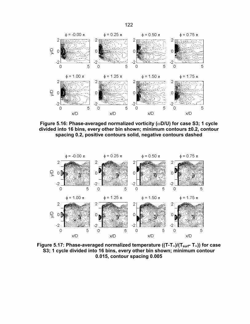
122
Figure 5.16: Phase-averaged normalized vorticity (�D/U) for case S3; 1 cycledivided into 16 bins, every other bin shown; minimum contours ±0.2, contour
spacing 0.2, positive contours solid, negative contours dashed
Figure 5.17: Phase-averaged normalized temperature ((T-T∞)/(Tsurf- T∞)) for caseS3; 1 cycle divided into 16 bins, every other bin shown; minimum contour
0.015, contour spacing 0.005

123
Figure 5.18: Mean and rms normalized velocity (u/U) and normalized vorticity(�D/U) for case S4; rms velocity contours are at 0.1 intervals; vorticity
contours are at 0.5 intervals, negative contours are dashed, positive contoursare solid
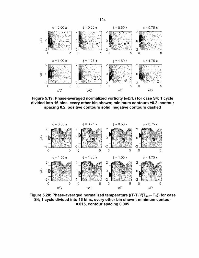
124
Figure 5.19: Phase-averaged normalized vorticity (�D/U) for case S4; 1 cycledivided into 16 bins, every other bin shown; minimum contours ±0.2, contour
spacing 0.2, positive contours solid, negative contours dashed
Figure 5.20: Phase-averaged normalized temperature ((T-T∞)/(Tsurf- T∞)) for caseS4; 1 cycle divided into 16 bins, every other bin shown; minimum contour
0.015, contour spacing 0.005

125
Figure 5.21: Mean and rms normalized velocity (u/U) and normalized vorticity(�D/U) for case S5; rms velocity contours are at 0.1 intervals; vorticity
contours are at 0.5 intervals, negative contours are dashed, positive contoursare solid

126
Figure 5.22: Phase-averaged normalized vorticity (�D/U) for case S5; 3 cyclesdivided into 48 bins, every other bin for 1st cycle shown; minimum contours±0.2, contour spacing 0.2, positive contours solid, negative contours dashed
Figure 5.23: Phase-averaged normalized temperature ((T-T∞)/(Tsurf- T∞)) for caseS5; 3 cycles divided into 48 bins, every other bin for 1sr cycle shown;
minimum contour 0.015, contour spacing 0.005

127
Figure 5.24: Phase-averaged vorticity (�D/U) for case S5; 3 cycles divided into48 bins, every other bin for 2nd cycle shown; minimum contours ±0.2, contour
spacing 0.2, positive contours solid, negative contours dashed
Figure 5.25: Phase-averaged normalized temperature ((T-T∞)/(Tsurf- T∞)) for caseS5; 3 cycles divided into 48 bins, every other bin for 2nd cycle shown;
minimum contour 0.015, contour spacing 0.005

128
Figure 5.26: Phase-averaged normalized vorticity (�D/U) for case S5; 3 cyclesdivided into 48 bins, every other bin for 3rd cycle shown; minimum contours±0.2, contour spacing 0.2, positive contours solid, negative contours dashed
Figure 5.27: Phase-averaged normalized temperature ((T-T∞)/(Tsurf- T∞)) for caseS5; 3 cycles divided into 48 bins, every other bin for 3rd cycle shown; minimum
contour 0.015, contour spacing 0.005

129
Figure 5.28: Mean and rms normalized velocity (u/U) and normalized vorticity(�D/U) for case S6; rms velocity contours are at 0.1 intervals; vorticity
contours are at 0.5 intervals, negative contours are dashed, positive contoursare solid

130
Figure 5.29: Phase-averaged normalized vorticity (�D/U) for case S6; 1 cycledivided into 16 bins, every other bin shown; minimum contours ±0.2, contour
spacing 0.2, positive contours solid, negative contours dashed
Figure 5.30: Phase-averaged normalized temperature ((T-T∞)/(Tsurf- T∞)) for caseS6; 1 cycle divided into 16 bins, every other bin shown; minimum contour
0.015, contour spacing 0.005

131
Figure 5.31: Mean and rms normalized velocity (u/U) and normalized vorticity(�D/U) for case S7; rms velocity contours are at 0.1 intervals; vorticity
contours are at 0.5 intervals, negative contours are dashed, positive contoursare solid

132
Figure 5.32: Phase-averaged normalized vorticity (�D/U) for case S7; 3 cyclesdivided into 48 bins, every other bin for 1st cycle shown; minimum contours±0.2, contour spacing 0.2, positive contours solid, negative contours dashed
Figure 5.33: Phase-averaged normalized temperature ((T-T∞)/(Tsurf- T∞)) for caseS7; 3 cycles divided into 48 bins, every other bin for 1st cycle shown; minimum
contour 0.015, contour spacing 0.005

133
Figure 5.34: Phase-averaged vorticity (�D/U) for case S7; 3 cycles divided into48 bins, every other bin for 2nd cycle shown; minimum contours ±0.2, contour
spacing 0.2, positive contours solid, negative contours dashed
Figure 5.35: Phase-averaged normalized temperature ((T-T∞)/(Tsurf- T∞)) for caseS7; 3 cycles divided into 48 bins, every other bin for 2nd cycle shown;
minimum contour 0.015, contour spacing 0.005

134
Figure 5.36: Phase-averaged normalized vorticity (�D/U) for case S7; 3 cyclesdivided into 48 bins, every other bin for 3rd cycle shown; minimum contours±0.2, contour spacing 0.2, positive contours solid, negative contours dashed
Figure 5.37: Phase-averaged normalized temperature ((T-T∞)/(Tsurf- T∞)) for caseS7; 3 cycles divided into 48 bins, every other bin for 3rd cycle shown; minimum
contour 0.015, contour spacing 0.005

135
Figure 5.38: Mean and rms normalized velocity (u/U) and normalized vorticity(�D/U) for case S8; rms velocity contours are at 0.1 intervals; vorticity
contours are at 0.5 intervals, negative contours are dashed, positive contoursare solid
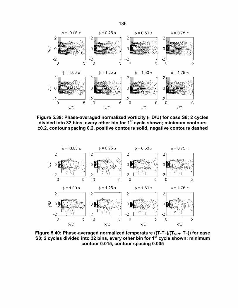
136
Figure 5.39: Phase-averaged normalized vorticity (�D/U) for case S8; 2 cyclesdivided into 32 bins, every other bin for 1st cycle shown; minimum contours±0.2, contour spacing 0.2, positive contours solid, negative contours dashed
Figure 5.40: Phase-averaged normalized temperature ((T-T∞)/(Tsurf- T∞)) for caseS8; 2 cycles divided into 32 bins, every other bin for 1st cycle shown; minimum
contour 0.015, contour spacing 0.005

137
Figure 5.41: Phase-averaged vorticity (�D/U) for case S8; 2 cycles divided into32 bins, every other bin for 2nd cycle shown; minimum contours ±0.2, contour
spacing 0.2, positive contours solid, negative contours dashed
Figure 5.42: Phase-averaged normalized temperature ((T-T∞)/(Tsurf- T∞)) for caseS8; 2 cycles divided into 32 bins, every other bin for 2nd cycle shown;
minimum contour 0.015, contour spacing 0.005

138
Figure 5.43: Mean and rms normalized velocity (u/U) and normalized vorticity(�D/U) for case S9; rms velocity contours are at 0.1 intervals; vorticity
contours are at 0.5 intervals, negative contours are dashed, positive contoursare solid

139
Figure 5.44: Phase-averaged normalized vorticity (�D/U) for case S9; 2 cyclesdivided into 32 bins, every other bin for 1st cycle shown; minimum contours±0.2, contour spacing 0.2, positive contours solid, negative contours dashed
Figure 5.45: Phase-averaged normalized temperature ((T-T∞)/(Tsurf- T∞)) for caseS9; 2 cycles divided into 32 bins, every other bin for 1st cycle shown; minimum
contour 0.015, contour spacing 0.005

140
Figure 5.46: Phase-averaged normalized vorticity (�D/U) for case S9; 2 cyclesdivided into 32 bins, every other bin for 2nd cycle shown; minimum contours±0.2, contour spacing 0.2, positive contours solid, negative contours dashed
Figure 5.47: Phase-averaged normalized temperature ((T-T∞)/(Tsurf- T∞)) for caseS9; 2 cycles divided into 32 bins, every other bin for 2nd cycle shown;
minimum contour 0.015, contour spacing 0.005

141
Figure 5.48: Mean and rms normalized velocity (u/U) and normalized vorticity(�D/U) for case S10; rms velocity contours are at 0.1 intervals; vorticity
contours are at 0.5 intervals, negative contours are dashed, positive contoursare solid

142
Figure 5.49: Phase-averaged normalized vorticity (�D/U) for case S10; 1 cycledivided into 16 bins, every other bin shown; minimum contours ±0.2, contour
spacing 0.2, positive contours solid, negative contours dashed
Figure 5.50: Phase-averaged normalized temperature ((T-T∞)/(Tsurf- T∞)) for caseS10; 1 cycle divided into 16 bins, every other bin shown; minimum contour
0.015, contour spacing 0.005

143
Figure 5.51: Mean and rms normalized velocity (u/U) and normalized vorticity(�D/U) for case S11; rms velocity contours are at 0.1 intervals; vorticity
contours are at 0.5 intervals, negative contours are dashed, positive contoursare solid

144
Figure 5.52: Phase-averaged normalized vorticity (�D/U) for case S11; 2 cyclesdivided into 32 bins, every other bin for 1st cycle shown; minimum contours±0.2, contour spacing 0.2, positive contours solid, negative contours dashed
Figure 5.53: Phase-averaged normalized temperature ((T-T∞)/(Tsurf- T∞)) for caseS11; 2 cycles divided into 32 bins, every other bin for 1st cycle shown;
minimum contour 0.015, contour spacing 0.005

145
Figure 5.54: Phase-averaged normalized vorticity (�D/U) for case S11; 2 cyclesdivided into 32 bins, every other bin for 2nd cycle shown; minimum contours±0.2, contour spacing 0.2, positive contours solid, negative contours dashed
Figure 5.55: Phase-averaged normalized temperature ((T-T∞)/(Tsurf- T∞)) for caseS11; 2 cycles divided into 32 bins, every other bin for 2nd cycle shown;
minimum contour 0.015, contour spacing 0.005
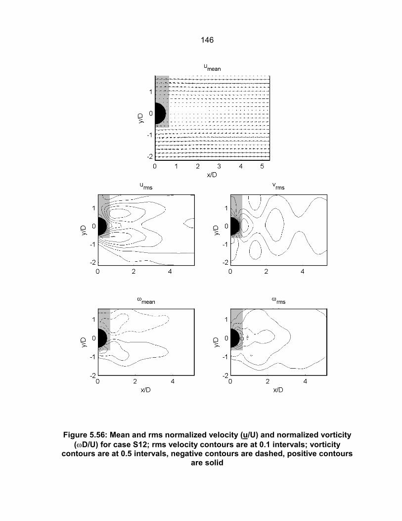
146
Figure 5.56: Mean and rms normalized velocity (u/U) and normalized vorticity(�D/U) for case S12; rms velocity contours are at 0.1 intervals; vorticity
contours are at 0.5 intervals, negative contours are dashed, positive contoursare solid

147
Figure 5.57: Phase-averaged normalized vorticity (�D/U) for case S12; 2 cyclesdivided into 32 bins, every other bin for 1st cycle shown; minimum contours±0.2, contour spacing 0.2, positive contours solid, negative contours dashed
Figure 5.58: Phase-averaged normalized temperature ((T-T∞)/(Tsurf- T∞)) for caseS12; 2 cycles divided into 32 bins, every other bin for 1st cycle shown;
minimum contour 0.015, contour spacing 0.005

148
Figure 5.59: Phase-averaged normalized vorticity (�D/U) for case S12; 2 cyclesdivided into 32 bins, every other bin for 2nd cycle shown; minimum contours±0.2, contour spacing 0.2, positive contours solid, negative contours dashed
Figure 5.60: Phase-averaged normalized temperature ((T-T∞)/(Tsurf- T∞)) for caseS12; 2 cycles divided into 32 bins, every other bin for 2nd cycle shown;
minimum contour 0.015, contour spacing 0.005

149
Figure 5.61: Mean and rms normalized velocity (u/U) and normalized vorticity(�D/U) for case S13; rms velocity contours are at 0.1 intervals; vorticity
contours are at 0.5 intervals, negative contours are dashed, positive contoursare solid
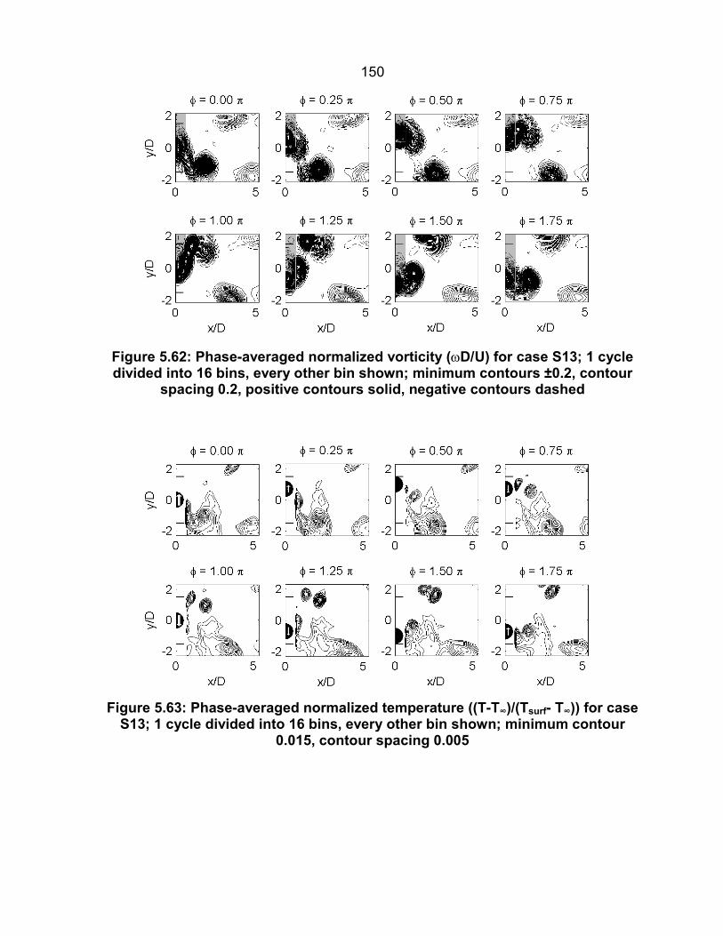
150
Figure 5.62: Phase-averaged normalized vorticity (�D/U) for case S13; 1 cycledivided into 16 bins, every other bin shown; minimum contours ±0.2, contour
spacing 0.2, positive contours solid, negative contours dashed
Figure 5.63: Phase-averaged normalized temperature ((T-T∞)/(Tsurf- T∞)) for caseS13; 1 cycle divided into 16 bins, every other bin shown; minimum contour
0.015, contour spacing 0.005

151
Figure 5.64: Mean and rms normalized velocity (u/U) and normalized vorticity(�D/U) for case S14; rms velocity contours are at 0.1 intervals; vorticity
contours are at 0.5 intervals, negative contours are dashed, positive contoursare solid

152
Figure 5.65: Phase-averaged normalized vorticity (�D/U) for case S14; 1 cycledivided into 16 bins, every other bin shown; minimum contours ±0.2, contour
spacing 0.2, positive contours solid, negative contours dashed
Figure 5.66: Phase-averaged normalized temperature ((T-T∞)/(Tsurf- T∞)) for caseS14; 1 cycle divided into 16 bins, every other bin shown; minimum contour
0.015, contour spacing 0.005

153
Figure 5.67: Mean and rms normalized velocity (u/U) and normalized vorticity(�D/U) for case S15; rms velocity contours are at 0.1 intervals; vorticity
contours are at 0.5 intervals, negative contours are dashed, positive contoursare solid

154
Figure 5.68: Phase-averaged normalized vorticity (�D/U) for case S15; 1 cycledivided into 16 bins, every other bin shown; minimum contours ±0.2, contour
spacing 0.2, positive contours solid, negative contours dashed
Figure 5.69: Phase-averaged normalized temperature ((T-T∞)/(Tsurf- T∞)) for caseS15; 1 cycle divided into 16 bins, every other bin shown; minimum contour
0.015, contour spacing 0.005

155
Figure 5.70: Mean and rms normalized velocity (u/U) and normalized vorticity(�D/U) for case S16; rms velocity contours are at 0.1 intervals; vorticity
contours are at 0.5 intervals, negative contours are dashed, positive contoursare solid

156
Figure 5.71: Phase-averaged normalized vorticity (�D/U) for case S16; 1 cycledivided into 16 bins, every other bin shown; minimum contours ±0.2, contour
spacing 0.2, positive contours solid, negative contours dashed
Figure 5.72: Phase-averaged normalized temperature ((T-T∞)/(Tsurf- T∞)) for caseS16; 1 cycle divided into 16 bins, every other bin shown; minimum contour
0.015, contour spacing 0.005

157
Figure 5.73: Mean and rms normalized velocity (u/U) and normalized vorticity(�D/U) for case S17; rms velocity contours are at 0.1 intervals; vorticity
contours are at 0.5 intervals, negative contours are dashed, positive contoursare solid

158
Figure 5.74: Phase-averaged normalized vorticity (�D/U) for case S17; 1 cycledivided into 16 bins, every other bin shown; minimum contours ±0.2, contour
spacing 0.2, positive contours solid, negative contours dashed
Figure 5.75: Phase-averaged normalized temperature ((T-T∞)/(Tsurf- T∞)) for caseS17; 1 cycle divided into 16 bins, every other bin shown; minimum contour
0.015, contour spacing 0.005

159
Figure 5.76: Mean and rms normalized velocity (u/U) and normalized vorticity(�D/U) for case S18; rms velocity contours are at 0.1 intervals; vorticity
contours are at 0.5 intervals, negative contours are dashed, positive contoursare solid

160
Figure 5.77: Phase-averaged normalized vorticity (�D/U) for case S18; 1 cycledivided into 16 bins, every other bin shown; minimum contours ±0.2, contour
spacing 0.2, positive contours solid, negative contours dashed
Figure 5.78: Phase-averaged normalized temperature ((T-T∞)/(Tsurf- T∞)) for caseS18; 1 cycle divided into 16 bins, every other bin shown; minimum contour
0.015, contour spacing 0.005

161
Figure 5.79: Mean and rms normalized velocity (u/U) and normalized vorticity(�D/U) for case S19; rms velocity contours are at 0.1 intervals; vorticity
contours are at 0.5 intervals, negative contours are dashed, positive contoursare solid

162
Figure 5.80: Phase-averaged normalized vorticity (�D/U) for case S19; 1 cycledivided into 16 bins, every other bin shown; minimum contours ±0.2, contour
spacing 0.2, positive contours solid, negative contours dashed
Figure 5.81: Phase-averaged normalized temperature ((T-T∞)/(Tsurf- T∞)) for caseS19; 1 cycle divided into 16 bins, every other bin shown; minimum contour
0.015, contour spacing 0.005

163
Figure 5.82: Mean and rms normalized velocity (u/U) and normalized vorticity(�D/U) for case S20; rms velocity contours are at 0.1 intervals; vorticity
contours are at 0.5 intervals, negative contours are dashed, positive contoursare solid

164
Figure 5.83: Phase-averaged normalized vorticity (�D/U) for case S20; 1 cycledivided into 16 bins, every other bin shown; minimum contours ±0.2, contour
spacing 0.2, positive contours solid, negative contours dashed
Figure 5.84: Phase-averaged normalized temperature ((T-T∞)/(Tsurf- T∞)) for caseS20; 1 cycle divided into 16 bins, every other bin shown; minimum contour
0.015, contour spacing 0.005

165
Figure 5.85: Mean and rms normalized velocity (u/U) and normalized vorticity(�D/U) for case S21; rms velocity contours are at 0.1 intervals; vorticity
contours are at 0.5 intervals, negative contours are dashed, positive contoursare solid

166
Figure 5.86: Phase-averaged normalized vorticity (�D/U) for case S21; 1 cycledivided into 16 bins, every other bin shown; minimum contours ±0.2, contour
spacing 0.2, positive contours solid, negative contours dashed
Figure 5.87: Phase-averaged normalized temperature ((T-T∞)/(Tsurf- T∞)) for caseS21; 1 cycle divided into 16 bins, every other bin shown; minimum contour
0.015, contour spacing 0.005

167
Figure 5.88: Mean and rms normalized velocity (u/U) and normalized vorticity(�D/U) for case S22; rms velocity contours are at 0.1 intervals; vorticity
contours are at 0.5 intervals, negative contours are dashed, positive contoursare solid
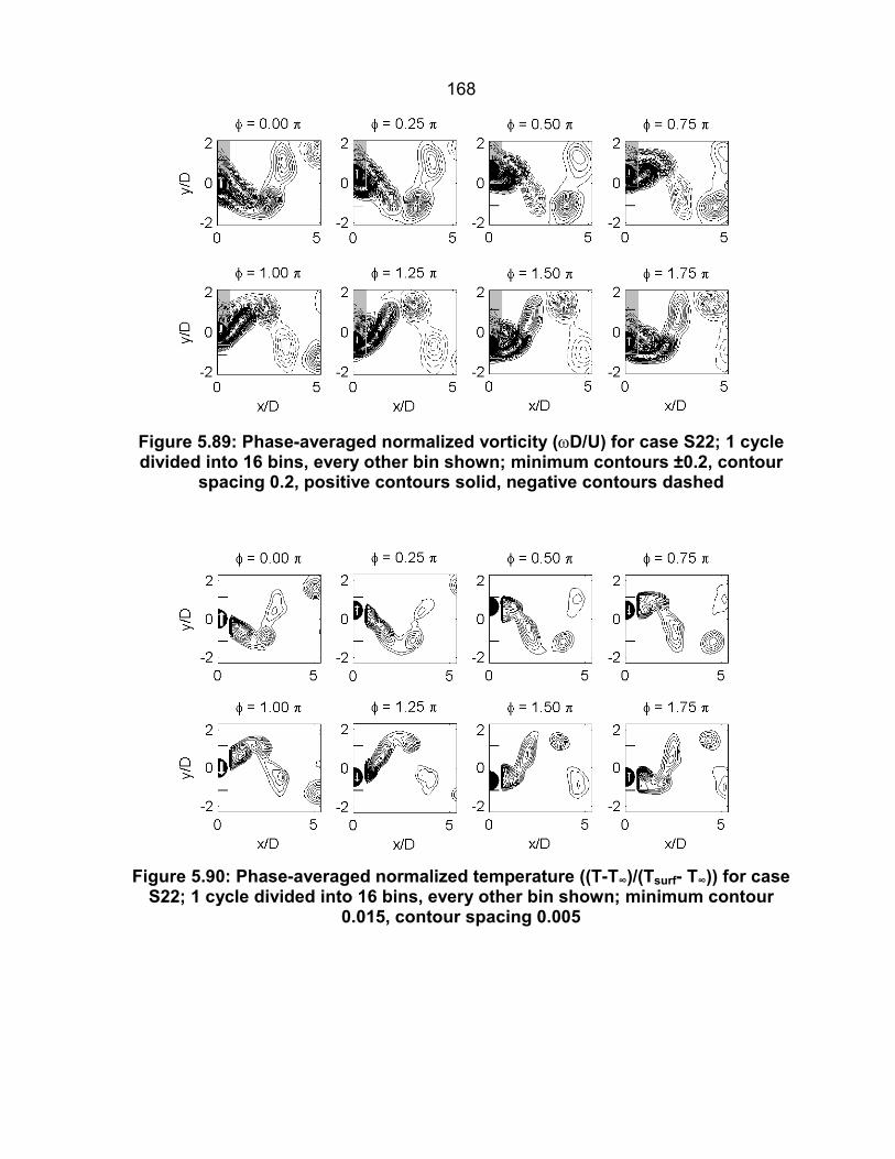
168
Figure 5.89: Phase-averaged normalized vorticity (�D/U) for case S22; 1 cycledivided into 16 bins, every other bin shown; minimum contours ±0.2, contour
spacing 0.2, positive contours solid, negative contours dashed
Figure 5.90: Phase-averaged normalized temperature ((T-T∞)/(Tsurf- T∞)) for caseS22; 1 cycle divided into 16 bins, every other bin shown; minimum contour
0.015, contour spacing 0.005

169
Figure 5.91: Mean and rms normalized velocity (u/U) and normalized vorticity(�D/U) for case S23; rms velocity contours are at 0.1 intervals; vorticity
contours are at 0.5 intervals, negative contours are dashed, positive contoursare solid

170
Figure 5.92: Phase-averaged normalized vorticity (�D/U) for case S23; 1 cycledivided into 16 bins, every other bin shown; minimum contours ±0.2, contour
spacing 0.2, positive contours solid, negative contours dashed
Figure 5.93: Phase-averaged normalized temperature ((T-T∞)/(Tsurf- T∞)) for caseS23; 1 cycle divided into 16 bins, every other bin shown; minimum contour
0.015, contour spacing 0.005

171
Figure 5.94: Mean and rms normalized velocity (u/U) and normalized vorticity(�D/U) for case S24; rms velocity contours are at 0.1 intervals; vorticity
contours are at 0.5 intervals, negative contours are dashed, positive contoursare solid

172
Figure 5.95: Phase-averaged normalized vorticity (�D/U) for case S24; 1 cycledivided into 16 bins, every other bin shown; minimum contours ±0.2, contour
spacing 0.2, positive contours solid, negative contours dashed
Figure 5.96: Phase-averaged normalized temperature ((T-T∞)/(Tsurf- T∞)) for caseS24; 1 cycle divided into 16 bins, every other bin shown; minimum contour
0.015, contour spacing 0.005

173
Figure 5.97: Mean and rms normalized velocity (u/U) and normalized vorticity(�D/U) for case S25; rms velocity contours are at 0.1 intervals; vorticity
contours are at 0.5 intervals, negative contours are dashed, positive contoursare solid

174
Figure 5.98: Phase-averaged normalized vorticity (�D/U) for case S25; 1 cycledivided into 16 bins, every other bin shown; minimum contours ±0.2, contour
spacing 0.2, positive contours solid, negative contours dashed
Figure 5.99: Phase-averaged normalized temperature ((T-T∞)/(Tsurf- T∞)) for caseS25; 1 cycle divided into 16 bins, every other bin shown; minimum contour
0.015, contour spacing 0.005

175
Figure 5.100: Mean and rms normalized velocity (u/U) and normalized vorticity(�D/U) for case S26; rms velocity contours are at 0.1 intervals; vorticity
contours are at 0.5 intervals, negative contours are dashed, positive contoursare solid

176
Figure 5.101: Phase-averaged normalized vorticity (�D/U) for case S26; 1 cycledivided into 16 bins, every other bin shown; minimum contours ±0.2, contour
spacing 0.2, positive contours solid, negative contours dashed
Figure 5.102: Phase-averaged normalized temperature ((T-T∞)/(Tsurf- T∞)) forcase S26; 1 cycle divided into 16 bins, every other bin shown; minimum
contour 0.015, contour spacing 0.005

177
Figure 5.103: Mean and rms normalized velocity (u/U) and normalized vorticity(�D/U) for case S27; rms velocity contours are at 0.1 intervals; vorticity
contours are at 0.5 intervals, negative contours are dashed, positive contoursare solid

178
Figure 5.104: Phase-averaged normalized vorticity (�D/U) for case S27; 1 cycledivided into 16 bins, every other bin shown; minimum contours ±0.2, contour
spacing 0.2, positive contours solid, negative contours dashed
Figure 5.105: Phase-averaged normalized temperature ((T-T∞)/(Tsurf- T∞)) forcase S27; 1 cycle divided into 16 bins, every other bin shown; minimum
contour 0.015, contour spacing 0.005

179
Figure 5.106: Mean and rms normalized velocity (u/U) and normalized vorticity(�D/U) for case S28; rms velocity contours are at 0.1 intervals; vorticity
contours are at 0.5 intervals, negative contours are dashed, positive contoursare solid

180
Figure 5.107: Phase-averaged normalized vorticity (�D/U) for case S28; 1 cycledivided into 16 bins, every other bin shown; minimum contours ±0.2, contour
spacing 0.2, positive contours solid, negative contours dashed
Figure 5.108: Phase-averaged normalized temperature ((T-T∞)/(Tsurf- T∞)) forcase S28; 1 cycle divided into 16 bins, every other bin shown; minimum
contour 0.015, contour spacing 0.005

181
Figure 5.109: Mean and rms normalized velocity (u/U) and normalized vorticity(�D/U) for case S29; rms velocity contours are at 0.1 intervals; vorticity
contours are at 0.5 intervals, negative contours are dashed, positive contoursare solid
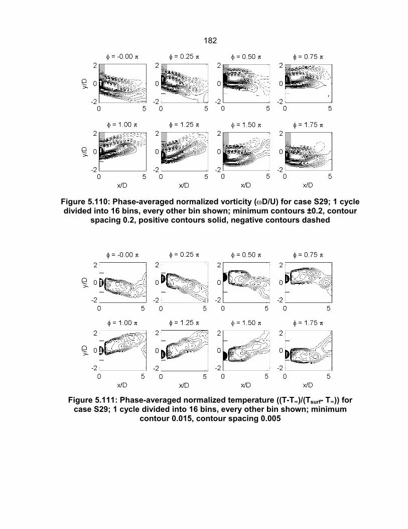
182
Figure 5.110: Phase-averaged normalized vorticity (�D/U) for case S29; 1 cycledivided into 16 bins, every other bin shown; minimum contours ±0.2, contour
spacing 0.2, positive contours solid, negative contours dashed
Figure 5.111: Phase-averaged normalized temperature ((T-T∞)/(Tsurf- T∞)) forcase S29; 1 cycle divided into 16 bins, every other bin shown; minimum
contour 0.015, contour spacing 0.005

183
Figure 5.112: Mean and rms normalized velocity (u/U) and normalized vorticity(�D/U) for case S30; rms velocity contours are at 0.1 intervals; vorticity
contours are at 0.5 intervals, negative contours are dashed, positive contoursare solid

184
Figure 5.113: Phase-averaged normalized vorticity (�D/U) for case S30; 1 cycledivided into 16 bins, every other bin shown; minimum contours ±0.2, contour
spacing 0.2, positive contours solid, negative contours dashed
Figure 5.114: Phase-averaged normalized temperature ((T-T∞)/(Tsurf- T∞)) forcase S30; 1 cycle divided into 16 bins, every other bin shown; minimum
contour 0.015, contour spacing 0.005

185
Figure 5.115: Mean and rms normalized velocity (u/U) and normalized vorticity(�D/U) for case L0; rms velocity contours are at 0.1 intervals; vorticity
contours are at 0.5 intervals, negative contours are dashed, positive contoursare solid

186
Figure 5.116: Mean and rms normalized velocity (u/U) and normalized vorticity(�D/U) for case L1; rms velocity contours are at 0.1 intervals; vorticity
contours are at 0.5 intervals, negative contours are dashed, positive contoursare solid

187
Figure 5.117: Phase-averaged normalized vorticity (�D/U) for case L1; 1 cycledivided into 16 bins, every other bin shown; minimum contours ±0.2, contour
spacing 0.2, positive contours solid, negative contours dashed

188
Figure 5.118: Mean and rms normalized velocity (u/U) and normalized vorticity(�D/U) for case L2; rms velocity contours are at 0.1 intervals; vorticity
contours are at 0.5 intervals, negative contours are dashed, positive contoursare solid

189
Figure 5.119: Phase-averaged normalized vorticity (�D/U) for case L2; 1 cycledivided into 16 bins, every other bin shown; minimum contours ±0.2, contour
spacing 0.2, positive contours solid, negative contours dashed

190
Figure 5.120: Mean and rms normalized velocity (u/U) and normalized vorticity(�D/U) for case L3; rms velocity contours are at 0.1 intervals; vorticity
contours are at 0.5 intervals, negative contours are dashed, positive contoursare solid

191
Figure 5.121: Phase-averaged normalized vorticity (�D/U) for case L3; 1 cycledivided into 16 bins, every other bin shown; minimum contours ±0.2, contour
spacing 0.2, positive contours solid, negative contours dashed

192
Figure 5.122: Mean and rms normalized velocity (u/U) and normalized vorticity(�D/U) for case L4; rms velocity contours are at 0.1 intervals; vorticity
contours are at 0.5 intervals, negative contours are dashed, positive contoursare solid

193
Figure 5.123: Phase-averaged normalized vorticity (�D/U) for case L4; 1 cycledivided into 16 bins, every other bin shown; minimum contours ±0.2, contour
spacing 0.2, positive contours solid, negative contours dashed

194
Figure 5.124: Mean and rms normalized velocity (u/U) and normalized vorticity(�D/U) for case L5; rms velocity contours are at 0.1 intervals; vorticity
contours are at 0.5 intervals, negative contours are dashed, positive contoursare solid

195
Figure 5.125: Phase-averaged normalized vorticity (�D/U) for case L5; 1 cycledivided into 16 bins, every other bin shown; minimum contours ±0.2, contour
spacing 0.2, positive contours solid, negative contours dashed

196
Figure 5.126: Mean and rms normalized velocity (u/U) and normalized vorticity(�D/U) for case L6; rms velocity contours are at 0.1 intervals; vorticity
contours are at 0.5 intervals, negative contours are dashed, positive contoursare solid

197
Figure 5.127: Phase-averaged normalized vorticity (�D/U) for case L6; 1 cycledivided into 16 bins, every other bin shown; minimum contours ±0.2, contour
spacing 0.2, positive contours solid, negative contours dashed

198
Figure 5.128: Mean and rms normalized velocity (u/U) and normalized vorticity(�D/U) for case L7; rms velocity contours are at 0.1 intervals; vorticity
contours are at 0.5 intervals, negative contours are dashed, positive contoursare solid

199
Figure 5.129: Phase-averaged normalized vorticity (�D/U) for case L7; 1 cycledivided into 16 bins, every other bin shown; minimum contours ±0.2, contour
spacing 0.2, positive contours solid, negative contours dashed

200
Figure 5.130: Mean and rms normalized velocity (u/U) and normalized vorticity(�D/U) for case L8; rms velocity contours are at 0.1 intervals; vorticity
contours are at 0.5 intervals, negative contours are dashed, positive contoursare solid

201
Figure 5.131: Phase-averaged normalized vorticity (�D/U) for case L8; 1 cycledivided into 16 bins, every other bin shown; minimum contours ±0.2, contour
spacing 0.2, positive contours solid, negative contours dashed

202
Figure 5.132: Mean and rms normalized velocity (u/U) and normalized vorticity(�D/U) for case L9; rms velocity contours are at 0.1 intervals; vorticity
contours are at 0.5 intervals, negative contours are dashed, positive contoursare solid

203
Figure 5.133: Phase-averaged normalized vorticity (�D/U) for case L9; 1 cycledivided into 16 bins, every other bin shown; minimum contours ±0.2, contour
spacing 0.2, positive contours solid, negative contours dashed

204
Figure 5.134: Mean and rms normalized velocity (u/U) and normalized vorticity(�D/U) for case L10; rms velocity contours are at 0.1 intervals; vorticity
contours are at 0.5 intervals, negative contours are dashed, positive contoursare solid

205
Figure 5.135: Phase-averaged normalized vorticity (�D/U) for case L10; 1 cycledivided into 16 bins, every other bin shown; minimum contours ±0.2, contour
spacing 0.2, positive contours solid, negative contours dashed

206
Figure 5.136: Mean and rms normalized velocity (u/U) and normalized vorticity(�D/U) for case L11; rms velocity contours are at 0.1 intervals; vorticity
contours are at 0.5 intervals, negative contours are dashed, positive contoursare solid

207
Figure 5.137: Phase-averaged normalized vorticity (�D/U) for case L11; 1 cycledivided into 16 bins, every other bin shown; minimum contours ±0.2, contour
spacing 0.2, positive contours solid, negative contours dashed
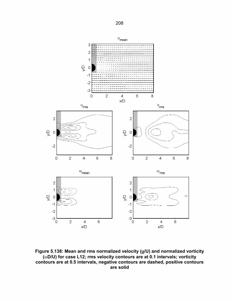
208
Figure 5.138: Mean and rms normalized velocity (u/U) and normalized vorticity(�D/U) for case L12; rms velocity contours are at 0.1 intervals; vorticity
contours are at 0.5 intervals, negative contours are dashed, positive contoursare solid

209
Figure 5.139: Phase-averaged normalized vorticity (�D/U) for case L12; 1 cycledivided into 16 bins, every other bin shown; minimum contours ±0.2, contour
spacing 0.2, positive contours solid, negative contours dashed

210
Figure 5.140: Mean and rms normalized velocity (u/U) and normalized vorticity(�D/U) for case L13; rms velocity contours are at 0.1 intervals; vorticity
contours are at 0.5 intervals, negative contours are dashed, positive contoursare solid

211
Figure 5.141: Phase-averaged normalized vorticity (�D/U) for case L13; 1 cycledivided into 16 bins, every other bin shown; minimum contours ±0.2, contour
spacing 0.2, positive contours solid, negative contours dashed
Figure 5.142: Normalized heat transfer coefficient (Nu/Nu0) vs. formationlength (�f) for all cases consisting of only single vortices (no pairs)

212
Figure 5.143: Phase-averaged velocity and normalized temperature((T-T∞)/(Tsurf- T∞)) for case S14; 1 cycle divided into 16 bins, every other bin
shown; minimum contour 0.015, contour spacing 0.01
Figure 5.144: Phase-averaged velocity and normalized temperature((T-T∞)/(Tsurf- T∞)) for case S17; 1 cycle divided into 16 bins, every other bin
shown; minimum contour 0.015, contour spacing 0.01

213
Figure 5.145: Phase-averaged velocity and normalized temperature((T-T∞)/(Tsurf- T∞)) for case S20; 1 cycle divided into 16 bins, every other bin
shown; minimum contour 0.015, contour spacing 0.01
Figure 5.146: Phase-averaged velocity and normalized temperature((T-T∞)/(Tsurf- T∞)) for case S23; 1 cycle divided into 16 bins, every other bin
shown; minimum contour 0.015, contour spacing 0.01

214
Figure 5.147: Normalized heat transfer coefficient (Nu/Nu0) vs. normalized rmstransverse velocity (Vrms/U) for cases S13, S18, S22 and S23
Figure 5.148: Normalized circulation and vortex shedding angle vs. normalizedrms transverse velocity (Vrms/U) for cases S13, S18, S22 and S23

215
6 Conclusion
There were two main goals of this study: to understand the mechanism by
which transverse cylinder oscillations modify the heat transfer from a heated circular
cylinder in cross-flow and to explore the dynamics of the vortex formation process in
the wake.
Two sets of experiments were carried out to accomplish these goals. In the
first set, the cylinder’s heat transfer coefficient was determined over a wide range of
oscillation conditions, and the results were compared to established relationships
between oscillation conditions and wake structure. The second set of experiments
used DPIT/V to measure the temperature and velocity fields in the near-wake for a
reduced set of cases. This allowed the vortex formation process and the effects of
wake structure on heat transfer to be examined directly. The particular cases
observed were chosen to be representative of the variety of wake structures that
exist for this type of flow. Based upon the results of this investigation, a number of
conclusions can be drawn.
First, heat transfer enhancement associated with oscillations at frequencies
near the Strouhal frequency and its harmonics is limited to amplitude ratios less than
about 0.5. For larger amplitude ratios, the cylinder heat transfer coefficient is
primarily determined by the wake mode and the transverse velocity. The role of
wake mode in determining the heat transfer coefficient was observed for the first
time. While previous authors have been unsuccessful at correlating the transverse
velocity with the heat transfer coefficient, it was shown in this investigation that

216within a particular wake mode and away from effects associated with the Strouhal
frequency, the transverse cylinder velocity is the primary factor responsible for
variations in heat transfer coefficient.
Two new mechanisms by which the wake structure affects the heat transfer
were identified. The dynamics of the vortex formation process, including the
movement of the vortices during roll-up, were found to affect the cylinder heat
transfer coefficient significantly. The dependence of heat transfer coefficient on wake
mode is explained by this mechanism. In addition, the spacing between shed
vortices in the streamwise direction was correlated with heat transfer coefficient for
the 2S mode. The streamwise spacing is believed to affect the heat transfer
coefficient by influencing the entrainment of freestream temperature fluid by vortices
as they are forming. In addition to these new mechanisms, the effect of roll-up
distance discovered by Park (1998) was observed.
The transverse cylinder velocity was found to have two effects on heat
transfer coefficient. For a fixed wake structure, the effectiveness of the wake
vortices at enhancing heat transfer depends on their circulation. Additional vorticity
produced by the cylinder’s transverse oscillation rolls up in the wake and is therefore
a factor in determining the circulation of the wake vortices. Transverse velocity also
turns the wake with respect to the freestream flow, thereby spreading the heat
transfer enhancement over a larger portion of the cylinder.
Aspect ratio appears to play a role in determining the heat transfer coefficient
mainly for non-oscillating cylinders and cases with weak synchronization of the wake
with the cylinder oscillations. Examinations of the wake structure at the mid-span for

217equivalent non-dimensional oscillation conditions revealed no significant differences
for the two aspect ratios used in this study. This suggests that the different levels of
heat transfer enhancement observed are due to end effects. An implication of this
observation is that the benefits of a high aspect ratio heat exchanger element may
be achievable using low aspect ratio oscillating elements. However, this idea
requires further testing over a wider range of aspect ratios.
A new phenomenon was discovered in which the wake structure switches
back and forth between distinct wake modes and between variations of the same
wake mode. Temperature induced variations in the fluid viscosity are believed to be
the cause of this mode-switching. It is hypothesized that this results in changes to
the vorticity flux and kinetic energy flux into the wake, thereby changing the wake
mode and the heat transfer coefficient. This discovery points to the role of viscosity
and of the shear layer fluxes in determining wake mode, and this may lead to
improved understanding of the vortex formation and pinch-off processes in wakes in
general. This has broad relevance to bluff-body flows and unsteady separated
flows, not just to heat transfer applications.
Additional research into mode-switching needs to be performed. Identifying
the criteria for the occurrence of mode-switching would reveal a great deal about
wake formation processes. The proposed model of the mode-switching mechanism
needs to be quantified and tested. Further experiments in fluids with different
viscosity-temperature relationships are needed. Also, numerical simulations in
which the temperature dependence of viscosity can be prescribed or eliminated
would be useful.

218
Appendix ADigital particle image thermometry/velocimetry
Digital particle image thermometry/velocimetry (DPIT/V) is a combination of
two techniques that allows the temperature field and the velocity field to be
measured simultaneously in a thin cross section of a flow. Digital particle image
velocimetry (DPIV) is a technique for determining the velocity field from consecutive
images of particles suspended in a flow using cross-correlations. For DPIV, the
color of the particles is not relevant, and experiments can be carried out using
monochromatic light and reflective or fluorescent particles. Digital particle image
thermometry (DPIT) refers to the extraction of temperature field information from the
color of thermochromic liquid crystal (TLC) particles, which change their reflected
wavelength with temperature, suspended in the flow. DPIT/V combines these two
techniques by using the TLC particles as both temperature indicators and flow
tracers.
DPIT/V is carried out by seeding the flow with TLC particles, illuminating a
cross section with a sheet of white light and digitally recording color images of the
illuminated particles. The images are then analyzed to determine the velocity and
temperature fields in the flow. The intensity field of the images, i.e., the black and
white image left when color information is removed, is used to determine the velocity
field through standard DPIV. The color information in the images is used to
determine the temperature field.
DPIV is the digital version of the particle image velocimetry technique and
was first used by Willert and Gharib (1991). They captured images of particle-

219seeded flows illuminated with a sheet of laser light using a video camera and
digitizer. Cross-correlations of small windows in consecutive images produced
displacement estimates, which were converted to velocities using the known time
separation between images. DPIV processing techniques have progress since this
initial implementation. A comparison of widely used DPIV processing techniques
can be found in McKenna and McGillis (2002).
DPIT depends upon the property of TLC that they selectively reflect light of a
particular wavelength. The TLC acts as a Bragg scattering volume grating with a
pitch determined by the arrangement of molecules. Individual molecules of TLC,
also called chiral nematic liquid crystals because of their structure, become arranged
in planes with the long axis of each molecule aligned in the same direction. The
alignment directions of adjacent planes of molecules are slightly rotated with respect
to one another. The distance normal to the planes required for a set of planes to
undergo 360° of rotation defines the grating pitch. This pitch depends on the inter-
plane separation distance and rotation angle, which both depend on temperature.
Bragg scattering results in incident light being scattered at angles that depend on the
wavelength of the light and the pitch of the grating. The apparent color of the TLC
therefore depends on the temperature and on the angle between the incident light
and the observer. Because the relationship between color and temperature is
sensitive to chemical composition and to the optical arrangement, it is necessary to
calibrate TLC for use in experiments. A complete discussion of TLC can be found in
Parsley (1991).

220TLC has been used extensively for measuring temperature on surfaces, and
in recent years has been dispersed within fluids as well. Perhaps the most familiar
examples of TLC on surfaces are “Mood Rings” and strip thermometers. The first
reported use of TLC applied to a surface for fluid mechanics research was in a
qualitative study by Klein (1968). More recently, TLC has been used to seed fluid
flows in order the measure the temperature field within the flow. Rhee et al. (1984)
pioneered this use, though their results were only qualitative. The DPIT technique in
its present form was introduced by Dabiri and Gharib (1991) and was used to
investigate the wakes of heated cylinders by Park et al. (2001).
The quantitative measurement of temperature fields using TLC has advanced
considerably in recent years. A review of various color decomposition schemes
used for TLC calibration is presented by Park (1998, §2.3). Sabatino et al. (2000)
introduced a calibration technique that accounts for variation in viewing and
illumination angles across the field of view for TLC applied to a surface. They
essentially calibrated each pixel of their video camera independently. Günther and
von Rohr (2002) dealt with the same viewing and illumination angle issues for fluid-
dispersed TLC particles using a telecentric imaging system. According to Park
(1998), the uncertainty in temperature for individual TLC particles is 5% to 20% of
the useful temperature range. A range of uncertainties is used because the
calibration curve is non-linear, so the uncertainty varies over the useful temperature
range. For 32 pixel by 32 pixel averaging windows, this uncertainty is reduced to 2%
to 10%.

221There are other techniques available that measure the velocity and
temperature field in a flow simultaneously. One common technique is the use two-
color planar laser induced fluorescence (PLIF) and DPIV simultaneously. In this
technique, the ratio of the intensities of two fluorescing dyes is related to
temperature. One example of the use of this technique is Seuntiens et al. (2001)
who studied the wake of a non-oscillating cylinder in a tow tank. While this
technique is effective, it is better suited to large temperature differences than to the
small temperature differences used in this study.

222
Appendix BSteady, one-dimensional model for estimating heat transfer
coefficient using embedded thermocouple data
An expression for the heat transfer coefficient is derived based upon the one-
dimensional physical model of the cylinder structure described in §2.6. The resulting
expression and the internal temperature distribution are then evaluated to determine
the impact of the one-dimensional assumption.
Heat transfer inside the cylinder is described by the conductive heat equation,
which in cylindrical coordinates is written as
in2
2
2
2
2 pzTT
r1
rTr
rr1k
tTC ��
�
���
�
�
��
�
��
�
� �
���
��
���
� , (B.1)
where T is temperature, t is time, r is the radial distance from the cylinder axis, � is
the angle in the plane perpendicular to the cylinder axis, and z is the coordinate
along the cylinder axis. The power input per unit volume, pin, is related to the total
power input, Pin, by
� �2a
2b
inin RRL
Pp��
� . (B.2)
For the model, L is taken to be the heated length of the cylinder plus the 6.35 mm
unheated length at the free end.
Assuming that the temperature depends only on the radial coordinate and is
steady, this equation becomes
0k
prTr
rr1 in ���
�
���
�
. (B.3)
With the appropriate values of pin and k, equation (A.1) applies to all four regions of

223the cylinder. From the steady-state assumption, it is apparent that the heat flux at
the surface must balance the power input
� �LR2
PTThdrdTk
d
insurf
Rrd
d�
�����
�
, (B.4)
where h is the convective heat transfer coefficient, Tsurf is the surface temperature of
the cylinder and T� is the freestream temperature. The steady-state assumption
also requires that the temperature is uniform in the region 0 � r � Ra, regardless of
the material properties in that region. Since the thermocouple is entirely contained
in region a, it is evident that
� � tcTrT � for aRr0 �� . (B.5)
The solutions for the separate regions must match at the region boundaries in order
to produce a continuous temperature distribution with finite heat flux.
The general solution of equation (B.1) is
� � � � BrlnAk
prrT in241
���� , (B.6)
where A and B are constants. Applying the boundary and matching conditions
yields the solution
� � tca TrT � , (B.7a)
� ����
�
���
�
��
�
��
��
���
����
����
����
�
���
��
����
�
�
�
���
a2a
2b
2a
2a
2b
2a
b
intcb R
rlnRR
RRRrR
21
k1
L2PTrT , (B.7b)
� ����
�
���
�
�
��
��
� �
���
����
����
����
�
�����
�
����
�
���
a
b2a
2b
2a
bbc
intcc R
RlnRR
R21
k1
Rrln
k1
L2PTrT , and (B.7c)
� ����
�
���
�
�
��
��
� �
���
����
����
����
�
�����
�
����
����
�
����
�
���
a
b2a
2b
2a
bb
c
ccd
intcd R
RlnRR
R21
k1
RRln
k1
Rrln
k1
L2PTrT , (B.7d)

224where the subscript on T indicates the region in which each equation applies. A plot
of this temperature profile is shown in Figure B.1 using realistic values for the
various parameters. Writing the surface temperature in terms of the thermocouple
temperature gives the relationship
���
�
���
�
��
�
��
��
���
����
����
����
�
�����
�
����
����
�
����
�
���
a
b2a
2b
2a
bb
c
cc
d
d
intcsurf R
RlnRR
R21
k1
RRln
k1
RRln
k1
L2PTT . (B.8)
Equation (B.8) expresses that the cylinder surface temperature differs from the
thermocouple temperature by an amount that depends linearly on the power input,
Pin. The constant multiplying Pin is only a function of the cylinder’s material
properties and dimensions.
Combining equation (B.4) with equation (B.8) yields the heat transfer
coefficient
��
���
�
���
�
�
��
��
� �
���
����
����
����
�
�����
�
����
����
�
����
�
��
��
TRRln
RRR
21
k1
RRln
k1
RRln
k1
L2PT
LR2P
h
a
b2a
2b
2a
bb
c
cc
d
d
intc
d
in
. (B.9)
This can be rewritten in the form
� �1
Ttcin
d CTTP
LR2h�
�� ���
����
���
, (B.10)
where C�T is a constant given by
���
�
���
�
�
��
��
� �
���
����
����
����
�
�����
�
����
����
�
����
���
�
a
b2a
2b
2a
bb
c
cc
d
ddT R
RlnRR
R21
k1
RRln
k1
RRln
k1RC . (B.11)
It is also possible to determine C�T through a calibration rather than using the
result of the one-dimensional model. Such a calibration may account for additional

225details of the setup that are not accounted for in the model. However, the principal
result that Ttc – Tsurf is proportional to Pin will be retained.
Since the heat transfer coefficient is not being measured directly, it is
necessary to determine the uncertainty associated with the value obtained as a
function of the measured quantity uncertainties. Working with equation (B.10), the
relevant partial derivatives are
� �
� �
� �� �
� �� �
� �� �
� � 22
Ttcin
d
T
T2
Ttcin
d
in
tcd
d
T2
Ttcin
d
in
tc
d
in
T2
Ttcin
d2in
tcd
in
tc
T2
Ttcin
d
in
d
tc
T2
Ttcin
d
in
d
tc
hCTTP
LR2C
h
and
hLhC1CTT
PLR2
PTTR2
Lh
,hRhC1CTT
PLR2
PTTL2
Rh
,hPhC1CTT
PLR2
PTTLR2
Ph
,hTT
hC1CTTP
LR2P
LR2Th
,hTT
hC1CTTP
LR2P
LR2Th
�����
����
��
��
�
�
�����
�
����
��
���
�
�
�����
�
����
��
���
�
�
����
�
����
��
��
�
�
��
����
�
����
��
�
�
�
��
�����
�
����
��
��
�
�
�
��
�
�
�
��
�
�
�
��
�
�
�
��
�
�
�
��
�
�
�
��
(B.12)
The relative uncertainty in the heat transfer coefficient is then given by the
expression
� �� �
2C
22
L
2
d
R2
in
P2
tc
2T
2T2
T
2h
T
dintc hLRPTT
hC1h �
� ����
�
�
��
�
�
��
� ��
���
� ��
���
� ��
�
�����
��
� �
�
�, (B.13)
where � represents the uncertainty in the quantity indicated by the subscript.
Equation (B.13) represents measurement uncertainties only and does not account
for any error produced by the assumptions used in developing the model.

226In order to evaluate the impact of the one-dimensional assumption on the
accuracy of the calculated heat transfer coefficient, the temperature profile produced
by this model was compared to a two-dimensional calculation of the internal cylinder
temperature using local heat transfer coefficient data from the literature.
Data from Gau et al. (1999) was used to estimate the local heat transfer
coefficient as a function of angular position for a non-oscillating cylinder (Figure 1.8).
The non-oscillating cylinder case was chosen because it had the largest difference
between the minimum and maximum local Nusselt numbers and was therefore
expected to depart the most from the one-dimensional assumption. This data was
from experiments in air at a Reynolds number of 1600, so the local Nusselt numbers
reported were scaled by Re0.466 and Pr1/3 following the correlation of Hilpert (1933) in
equation (1.9). A 3rd order polynomial least-squares fit in �2 was used to represent
the scaled data analytically.
The two-dimensional calculation was carried out using the MATLAB PDE
Toolbox. A model was constructed having the same geometry, dimensions, and
physical properties as the one-dimensional model for the AR = 14.2 cylinder. The
boundary condition was specified using the previously mentioned polynomial fit to
the scaled data as the local heat transfer coefficient. The steady heat equation in
two dimensions was then solved, and the temperature at each grid point was
determined. As expected, the temperature field was not axisymmetric, and the
temperature was higher on the trailing half of the cylinder surface than on the
leading half. The average heat transfer coefficient was then calculated by averaging

227the temperature at all grid points located on the cylinder surface and applying
equation (1.7).
For comparison, equation (B.9) was solved to find the expected Ttc
corresponding to the average heat transfer coefficient. This value was then used in
equations (B.7a-d) to find the temperature profile for all radii inside the cylinder.
Figure B.2 shows the difference between the temperature for every grid point in the
two-dimensional calculation and the temperature at the corresponding radius from
the one-dimensional model. The two-dimensional solution forms an asymmetric but
organized scatter around the one-dimensional solution.
An upper bound was placed on the relative error of the one-dimensional
model using this calculation. The temperature at the smallest radius in the two-
dimensional solution was taken as Ttc and used to calculate the heat transfer
coefficient using the one-dimensional model. The resulting value was 1.9% less
than the heat transfer coefficient of the two-dimensional calculation. Assuming that
the local heat transfer coefficient for the non-oscillating case is the furthest from
axisymmetric of any case, this places an upper bound on the error associated with
the one-dimensional assumption. This small relative error is on the same order as
other sources of uncertainty in the experiment.
It is also possible to think of the resulting error as an offset in the measured
thermocouple temperature. The temperature at the smallest radius in the two-
dimensional calculation is 0.1°C above the thermocouple temperature that
corresponds to the correct average heat transfer coefficient. Since the

228thermocouple itself has an uncertainty of ±0.1°C, it is unlikely that the one-
dimensional assumption will affect the results in any significant way.

229
Figure B.1: Cylinder internal temperature profile using axisymmetric modelwith dimensions for large diameter cylinder and h = 1700 W/m2K

230
Figure B.2: Difference between cylinder temperatures calculated for one- andtwo-dimensional models for all angular coordinates

231
Appendix C Unsteady, one-dimensional model of cylinder response to step
change in heat transfer coefficient and determination of thecylinder thermal time constant
An unsteady, one-dimensional model of heat transfer inside the cylinder is
developed in order to evaluate the time scale of temperature changes when the
cylinder is subjected to a step change in heat transfer coefficient.
Starting from the same geometry as the steady model and equation (B.1), the
temperature is again assumed to be independent of � and z, but now the time
dependence is retained. This yields the equation
in2
2in
2
2
pkr
Tr1
rT
Cp
rT
r1
rT
Ck
tT �
����
����
�
�
�
����
�
����
�
�
���
����
�
�
, (C.1)
where T = T(r,t) and � is the thermal diffusivity. The initial and boundary conditions
are chosen to represent a situation where the heat transfer coefficient undergoes a
step change, such that
���
�
��
0t,h0t,h
hf
i , (C.2)
where the subscripts i and f indicate the initial and final states. Combining equation
(B.9) with equations (B.7a-d) and setting h = hi gives the initial condition T(r,0) =
Ti(r). The boundary conditions are given by
� �� �
0rT
Tt,RThrTk
0r
dfRr
dd
��
�
���
��
�
�
� . (C.3)

232Equation (C.1) can be simplified by making the substitution
� � � � � �rTt,rT~t,rT i�� , (C.4)
where T~ is the difference between the instantaneous temperature and the initial
condition. The governing equation becomes
��
�
�
��
�
�
�
��
�
�
�
�
rT~
r1
rT~
tT~
2
2
(C.5)
by using the fact that the power input and the initial condition form a solution to the
steady equation (equation B.3). Using the steady solution boundary condition that
� �� ��
�
��� TRThdrdTk dii
Rr
id
d
, (C.6)
the boundary condition at the surface becomes
� � � � � �� ��
�
�����
�� TRThht,RT~h
rT~k diifdf
Rr
d
d
, (C.7)
where the second term on the right hand side is a constant. At the center of the
cylinder, the boundary condition remains
0rT~
0r
��
�
�
. (C.8)
Though equation (C.5) is separable, the surface boundary condition (equation
C.7) is not. Therefore, the unsteady model was solved numerically for a variety of
heat transfer coefficients. It was found that the temperature at any particular radius
exponentially approaches the longtime solution after a brief initial period of about 1 -
3 seconds for the AR = 14.2 cylinder, and about 1 - 2 sec for the AR = 21.3 cylinder.

233Figure C.1 shows the temperature at the cylinder surface and on the cylinder axis for
one particular case.
Since the initial time is short compared to the time scale of the exponential
decay for both cylinders, it is disregarded in determining the thermal time constant
for the cylinders. The thermal time constant, �, is defined as the time required for
the difference between the instantaneous temperature at a point to decay to 1/e
times the initial difference at that point, such that
� � � �� � � � e
1t,rTrTt,rT,rT
i
�
���
���� . (C.9)
The longtime solution is taken to be the solution of the steady model for h = hf.

234
Figure C.1: Normalized surface and axial temperatures vs. time for model ofcylinder subjected to step change in heat transfer coefficient using properties
of the AR = 14.2 cylinder with Nuf/Nu0 = 2.38

235
References
Bishop, R. E. D. and Hassan, A. Y. 1964. The lift and drag forces on a circularcylinder oscillating in a flowing fluid. Proceedings of the Royal Society (London)Series A 277:51-75.
Brika, D. and Laneville, A. 1993. Vortex-induced vibrations of a long flexible circularcylinder. Journal of Fluid Mechanics 250:481-508.
Carberry, J., Sheridan, J. and Rockwell, D. 2001. Forces and wake modes of anoscillating cylinder. Journal of Fluids and Structures 15:523-532.
Cheng, C.-H., Chen, H.-N. and Aung, W. 1997. Experimental study of the effect oftransverse oscillation on convection heat transfer from a circular cylinder. Journal ofHeat Transfer 119:474-482.
Cheng, C.-H. and Hong, J.-L. 1997. Numerical prediction of lock-on effect onconvective heat transfer from a transversely oscillating circular cylinder.International Journal of Heat and Mass Transfer 40(8):1825-1834.
Dabiri, D. and Gharib, M. 1991. Digital particle image thermometry: The method andimplementation. Experiments in Fluids 11:77-86.
Gau, C., Wu, J. M. and Liang, C. Y. 1999. Heat transfer enhancement and vortexflow structure over a heated cylinder oscillating in the crossflow direction. Journal ofHeat Transfer 121:789-795.
Gharib, M., Rambod, E. and Shariff, K. 1998. A universal time scale for vortex ringformation. Journal of Fluid Mechanics 360:121-140.
Hilpert, R. 1933. Forsch. Geb. Ingenieurwes., 4, 215.
Incropera, F. P. and Dewitt, D. P. 1996. Fundamentals of Heat and Mass Transfer,4th ed., John Wiley and Sons, New York.
Jeon, D. and Gharib, M. 2003. (pre-print) On the relationship between the vortexformation process and cylinder wake vortex patterns. Journal of Fluid Mechanics.
Karanth, D., Rankin, G. W. and Sridhar, K. 1994. A finite difference calculation offorced convective heat transfer from an oscillating cylinder. International Journal ofHeat and Mass Transfer 37(11):1619-1630.
Kezios, S. P. and Prasanna, K. V. 1966. Effect of vibration on heat transfer from acylinder in normal flow. ASME Paper No. 66-WA/HT-43.

236Khalak, A and Williamson, C. H. K. 1999. Motions, forces and mode transitions invortex-induced vibrations at low mass-damping. Journal of Fluids and Structures13:813-851.
Klein, E. J. 1968. Application of liquid crystal to boundary layer flow visualization.AIAA Paper No.68-376.
McKenna, S. P. and McGillis, W. R. 2002. Performance of digital image velocimetryprocessing techniques. Experiments in Fluids 32(1):106-115.
Norberg, C. 1994. An experimental investigation of the flow around a circularcylinder: influence of aspect ratio. Journal of Fluid Mechanics 258:287-316.
Norberg, C. 2003. Fluctuating lift on a circular cylinder: review and newmeasurements. Journal of Fluids and Structures 17:57-96.
Park, H. G. 1998. A Study of Heat Transfer Processes in the Wake of a Stationaryand Oscillating Circular Cylinder Using Digital Particle Image Velocimetry /Thermometry. Ph.D. Thesis, California Institute of Technology.
Park, H. G., Dabiri, D. and Gharib, M. 2001. Digital particle imagevelocimetry/thermometry and application to the wake of a heated circular cylinder.Experiments in Fluids 30:327-338.
Parsley, M. 1991. The Hallcrest Handbook of Thermochromic Liquid CrystalTechnology, Hallcrest, Glenview, IL.
Perry, A.E. and Fairlie, B.D. 1974. Critical points in flow patterns. Advances inGeophysics, 18B:299-315.
Pottebaum, T. S. and Gharib, M. 2003. (submitted) The pinch-off process in astarting buoyant plume. Experiments in Fluids.
Rhee, H. S., Koseff, J. R. and Street, R. L. 1984. Flow visualization of arecirculating flow by rheoscopic liquid and liquid crystal techniques. Experiments inFluids 2:57-64.
Sabatino, D. R., Praisner, T. J. and Smith, C. R. 2000. A high-accuracy calibrationtechnique for thermochromic liquid crystal temperature measurements. Experimentsin Fluids 28:497-505.
Saxena, U. C. and Laird, A. D. K. 1978. Heat transfer from a cylinder oscillating in across-flow. Journal of Heat Transfer 100:684-689.

237Seuntiens, H. J., Kieft, R. N., Rindt, C. C. M. and van Steenhoven, A. A. 2001. 2Dtemperature measurements in the wake of a heated cylinder using LIF. Experimentsin Fluids 31:588-595.
Sreenivasan, K. and Ramachandran, A. 1961. Effect of vibration on heat transferfrom a horizontal cylinder to a normal air stream. International Journal of Heat andMass Transfer 3:60-67.
Taneda, S. 1956. Experimental investigation of the wakes behind cylinders andplates at low Reynolds numbers, Journal of Physical Society of Japan, 11, p. 302.
Willert, C. E. and Gharib, M. 1991. Digital particle image velocimetry. Experimentsin Fluids 10:181-193.
Williamson, C. H. K. and Roshko, A. 1988. Vortex formation in the wake of anoscillating cylinder. Journal of Fluids and Structures 2:355-381.
Zhukauskas, A. 1972. “Heat transfer from tubes in cross flow,” in Hartnett, J.P. andIrvine, T.F. Jr., Eds., Advances in Heat Transfer, Vol. 8, Academic Press, New York.