THESIS

ESTIMATING SPARSE INVERSE COVARIANCE MATRIX FOR BRAIN

COMPUTER INTERFACE APPLICATIONS

Submitted by

Annamalai Natarajan

Department of Computer Science

In partial fulfillment of the requirements

for the Degree of Master of Science

Colorado State University

Fort Collins, Colorado

Fall 2009

Copyright c© Annamalai Natarajan 2009All Rights Reserved

COLORADO STATE UNIVERSITY

October 9, 2009

WE HEREBY RECOMMEND THAT THE THESIS PREPARED UNDER

OUR SUPERVISION BY ANNAMALAI NATARAJAN ENTITLED ESTIMATING

SPARSE INVERSE COVARIANCE MATRIX FOR BRAIN COMPUTER INTER-

FACE APPLICATIONS BE ACCEPTED AS FULFILLING IN PART REQUIRE-

MENTS FOR THE DEGREE OF MASTER OF SCIENCE.

Committee on Graduate Work

Committee Member

Committee Member

Advisor

Co-Advisor

Acting Department Chair

ii

ABSTRACT OF THESIS

ESTIMATING SPARSE INVERSE COVARIANCE MATRIX FOR BRAIN

COMPUTER INTERFACE APPLICATIONS

In this project we present a brain-computer interface (BCI) which recognizes one

task from another in a timely manner. We use quadratic discriminant analysis to classify

Electroencephalography (EEG) samples in an online fashion. The raw EEG samples

are collected over half second intervals to estimate the power spectral densities. The

estimated power spectral densities are treated as individual samples by the classifier.

The mean and inverse covariance matrix parameters in the classifier are updated incre-

mentally as samples arrive spread over several training sessions. We also perform some

feature selection using only descriptive statistics of the collected data to throw away

irrelevant and redundant features. We have constrained the tasks to be imagination of

actual tasks to ready the BCI for real world applications. We evaluated the performance

of the BCI on two experiments. In experiment I the BCI achieves a moderate 74% clas-

sification accuracy when recognizing a right hand task from a visual spinning task. In

experiment II it achieves a poor performance of 57% when classifying a right hand task

from left foot.

Annamalai NatarajanDepartment of Computer ScienceColorado State UniversityFort Collins, CO 80523Fall 2009

iii

ACKNOWLEDGMENTS

I would like to thank my advisor, Dr. Charles Anderson, for his constant support

and guidance rendered during this thesis work. Special thanks to Dr. Patricia Davies for

showing me a different perspective of the human brain. I am grateful to Dr. Michael

Kirby for serving on my committee. I would like to thank Dr. William Gavin for many

fruitful discussions. I would also like to thank Asbjørn Berge, Are C. Jensen, and Anne

H. Schistad Solberg for their help with the incremental QDA algorithm. Lastly I would

like to thank my friends and family for their support.

iv

TABLE OF CONTENTS

1 Introduction 1

2 Background 6

3 Methods 11

3.1 Brain Computer Interface Architecture . . . . . . . . . . . . . . . . . . . . 11

3.2 EEG Data . . . . . . . . . . . . . . . . . . . . . . . . . . . . . . . . . . . 13

3.3 Power Spectral Density Estimation . . . . . . . . . . . . . . . . . . . . . . 15

3.4 Incremental QDA Algorithm . . . . . . . . . . . . . . . . . . . . . . . . . 20

3.5 Divergence between Computed and Estimated parameter distributions . . . 26

3.6 Feature Selection . . . . . . . . . . . . . . . . . . . . . . . . . . . . . . . 28

3.6.1 The Relief Algorithm . . . . . . . . . . . . . . . . . . . . . . . . . . . . 29

3.6.2 Preprocessing . . . . . . . . . . . . . . . . . . . . . . . . . . . . . . . . 30

4 Results 33

4.1 Experiment I . . . . . . . . . . . . . . . . . . . . . . . . . . . . . . . . . 33

4.2 Experiment II . . . . . . . . . . . . . . . . . . . . . . . . . . . . . . . . . 45

4.3 Comparison of Execution Time . . . . . . . . . . . . . . . . . . . . . . . . 50

5 Conclusion and Future Work 53

References 56

v

LIST OF FIGURES

1.1 Discriminant analysis . . . . . . . . . . . . . . . . . . . . . . . . . . . . . 3

2.1 The human brain [6] . . . . . . . . . . . . . . . . . . . . . . . . . . . . . 7

2.2 EEG frequencies [10] . . . . . . . . . . . . . . . . . . . . . . . . . . . . . 9

3.1 The Brain Computer Interface architecture . . . . . . . . . . . . . . . . . . 12

3.2 The 10-20 system of placement of electrodes [16] . . . . . . . . . . . . . . 14

3.3 Sample EEG data from 19 channels . . . . . . . . . . . . . . . . . . . . . 15

3.4 Sliding Hanning window over half second of EEG data . . . . . . . . . . . 18

3.5 Sample PSD estimates for a Right hand (right) and Left foot (left) tasks . . 19

3.6 Normalcy of PSD estimates. Sample QQ Plots for Fp1 and T4 channel

electrode PSD estimates . . . . . . . . . . . . . . . . . . . . . . . . . 21

3.7 The Inverse Covariance matrix for a small 5 feature dataset . . . . . . . . . 26

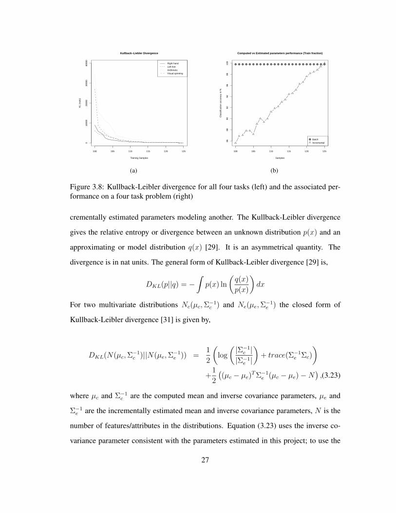
3.8 Kullback-Leibler divergence for all four tasks (left) and the associated per-

formance on a four task problem (right) . . . . . . . . . . . . . . . . . 27

4.1 Experiment I performance plot . . . . . . . . . . . . . . . . . . . . . . . . 36

4.2 Experiment I 1 to 1500 features heat map . . . . . . . . . . . . . . . . . . 38

4.3 Experiment I 400 to 1300 features heat map . . . . . . . . . . . . . . . . . 40

4.4 Experiment I PSD’s of F3 and F4 electrodes for the right hand task on the

train partition . . . . . . . . . . . . . . . . . . . . . . . . . . . . . . . 42

4.5 Experiment I F4 at 6-7 Hz (left) and F4 at 21-24 Hz (right) . . . . . . . . . 44

4.6 Experiment I F3 at 6-7 Hz (left) and F3 at 21-24 Hz (right) . . . . . . . . . 45

vi

4.7 Experiment I P3 at 6-7 Hz (left) and P3 at 21-24 Hz (right) . . . . . . . . . 46

4.8 Experiment II performance plot . . . . . . . . . . . . . . . . . . . . . . . . 46

4.9 Experiment II 500 to 1100 features heat map . . . . . . . . . . . . . . . . . 48

4.10 Experiment II 2000 to 2600 features heat map . . . . . . . . . . . . . . . . 49

4.11 Comparison of execution time taken to compute the inverse covariance matrix 52

vii

LIST OF TABLES

4.1 Comparison of performances on test partition for experiment I . . . . . . . 39

4.2 Comparison of performances on Test partition for experiment II . . . . . . 47

5.1 Time Embedded lag and skip on a sample dataset . . . . . . . . . . . . . . 54

viii

Chapter 1

Introduction

A human machine interface serves as a medium of communication between humans

and external devices. The brain-computer interface is a form of human machine inter-

face that helps connect the brain to external devices. The connection is typically via a

computer system to process, infer and translate users’ intentions into actions. Wolpaw,

et al., define BCI as a communication system that does not depend on the brain’s normal

output pathways of peripheral nerves and muscles [1]. BCI’s in offline mode operate

in two phases: training and testing. In the training phase the subjects perform different

tasks (imagine moving hands, feet, doing simple math, etc) and the BCI is trained to

recognize one task from another. In the testing phase the already trained BCI is tested

on new data for their generalization capability and performance. Besides numerous

challenges like the quality of Electroencephalography (EEG) signals (its non-stationary

nature, neurons firing property, convoluted cerebral cortex, all explained in Chapter 2),

common EEG artifacts [2] and also the underlying brain activity in actual and imagery

tasks, the BCI still qualifies as a medium of communication for subjects with locked in

syndrome. BCI’s are pursued with active interest in subjects with amyotrophic lateral

sclerosis (ALS), stroke, high level spinal cord injury, cerebral palsy or amputation. They

could also assist or aid in identification of human cognitive and sensory motor functions.

BCI’s equipped with EEG for data collection are easy to setup, can be deployed

1

in numerous environments, are preferred for their lack of risk and are inexpensive.

Other techniques used to map brain activation are functional magnetic resonance imag-

ing (fMRI), positron emission tomography (PET) and magnetoencephalography (MEG).

fMRI measures the changes in blood flow level (blood oxygen level dependent (BOLD)

level) in the brain. In PET a tracer isotope is injected into the subject that emits gamma

rays when it annihilates, these gamma rays are further traced by placing the subject

under a scanner. These approaches have relatively poor time resolution but excellent

space resolution when compared to EEG. MEG is an imaging technique that measures

the magnetic fields produced by electrical activity; EEG can be simultaneously recorded

along with MEG.

Clearly, from the description above, it can be noted that the BCI is a classification

problem. It will need to recognize one task from another for it to function efficiently.

In artificial intelligence (AI), machine learning approaches are broadly classified into

supervised, unsupervised and reinforcement learning. In supervised learning the train-

ing data is accompanied by target vectors, in unsupervised learning no target vectors are

provided; the goal is to group the training data into clusters. Reinforcement learning

is finding suitable actions in environments to maximize rewards. In our approach we

use supervised learning to train the BCI with training fraction samples and associated

target vectors and then test for its generalization capability. No matter what the learn-

ing approach is, the choice of an appropriate algorithm plays a crucial role. Factors

like algorithm complexity, computational complexity, number of parameters, ease of

implementation and memory requirements determine the choice of algorithms. Several

machine learning algorithms, in no particular order, like discriminant analysis, support

vector machines (SVM), hidden markov models (HMM), multilayer perceptrons, Bayes

classifier, principal component analysis (PCA), independent component analysis (ICA),

K nearest neighbors (kNN), common spatial pattern (CSP) and expectation maximiza-

2

tion (EM) have enjoyed success in BCI applications.

Figure 1.1: Discriminant analysis

In our approach we have implemented a variation of discriminant analysis called the

quadratic discriminant analysis (QDA). The general idea of discriminant analysis is to

find a combination of features that best discriminates one task from another. Figure 1.1

captures the idea of discriminant analysis in a two class problem. Class 1 is concentrated

in the center and class two is scattered around. The circle serves as the discriminatory

function; any sample falling inside the circle belongs to class 1 otherwise it belongs to

class 2. In QDA the combination of features is quadratic. The basic assumption in QDA

is that the data from each each class is normally distributed. It computes two parameters

per task, the mean and the covariance, from the train data using them in a discriminant

function to determine the target class. The limits of this approach are its generalization

3

capability and the time taken to compute the parameters. It takes a fairly large time for

large datasets. Considering the QDA for a BCI application, where subsequent training

sessions have been demonstrated to be successful [3, 4, 5], it would be more efficient if

the parameters could be updated in subsequent sessions rather then computing it from

scratch; this will also prove to be time saving in real world deployment. This is pre-

cisely the idea behind incremental QDA where we estimate the parameters rather than

computing them. From pilot experiments it appears that the estimated parameters are

close to the computed parameters when the number of samples is large. In terms of

performance the regular (using computed parameters) and incremental (using estimated

parameters) approaches converge. In addition to estimating the parameters we also per-

form some feature selection to improve the recognition rates as not all features are likely

to contribute to recognition of all the tasks.

The objectives of this project are summarized under two hypothesis below,

Hypothesis I

• Experiment with an incremental way to update mean and inverse covariance pa-

rameters

• The recognition rates of the incremental QDA should be comparable or better than

batch QDA (parameters are computed)

• The incremental QDA approach should be time efficient

Hypothesis II

• Feature Selection should improve the BCI performance significantly

• Feature Selection Should also minimize the number of parameters (i.e. inverse

covariance matrix entries thereby making it sparse) to be estimated

4

The rest of this report is organized as follows. Chapter 2 gives a brief overview of the

human brain and associated activities. Chapter 3 outlines the brain-computer interface

architecture and explains each component in detail. Chapter 4 evaluates the performance

of the BCI. Chapter 5 concludes this report and highlights the directions on future work.

5

Chapter 2

Background

This chapter is a brief introduction to the human brain from a neuroscience perspective.

We also outline the source of EEG activity and give an overview of BCI models.

The human brain is the site of consciousness, allowing humans to think, learn and

create. The brain is broadly divided into the cerebrum, cerebellum, limbic system and

the brain stem. The cerebrum is covered with a symmetric convoluted cortex with a left

and right hemispheres. The brain stem is located below the cerebrum and the cerebellum

is located beneath the cerebrum and behind the brain stem. The limbic system which

lies at the core of the brain contains the thalamus and hypothalamus among other parts.

Anatomists divide the cerebrum into Frontal, Parietal, Temporal and Occipital lobes.

These lobes inherit their names from the bones of the skull that overlie them. It is gener-

ally agreed that the Frontal lobe is associated with planning, problem solving, reasoning,

parts of speech, bodily movement and coordination. The Parietal lobe is associated with

bodily movement, orientation and recognition (such as touch, taste, pressure, pain, heat,

cold, etc). The Temporal lobe is associated with perception, auditory stimuli, memory

and speech. The Occipital lobe is associated with visual stimuli. Figure 2.1 is an image

of human brain with the lobes and their associated functions.

The brain is made up of approximately 100 billion neurons. Neurons are nerve

cells with dendrite and axon projections that take information to and from the nerve

6

Figure 2.1: The human brain [6]

cells, respectively. These neurons have a resting potential, typically between -70 to -

65 microvolts, which is the difference between the interior potential of the cell and the

extra cellular space. A stimulus triggers an action potential in the neuron which sends

out information (also know as firing property, impulse, spike) along the axons. Neurons

transmit messages electrochemically. A neuron fires only when its resting potential

drops below a threshold of -55 microvolts. A spiking neuron triggers another neuron

to spike and in turn another. This causes the resting potential to fluctuate as a result of

impulses arriving from other neurons at contact points (synapses). These impulses result

in post synaptic potentials which cause electric current to flow along the membrane of

the cell body and dendrites. This is the source of brain electric current. Brain electrical

current consists mostly of Na+, K+, Ca++, and Cl- ions. Only large populations of

7

active neurons can generate electrical activity strong enough to be detected at the scalp as

neurons tend to line up to fire. The Electroencephalogram is defined as electrical activity

of an alternating type recorded from the scalp surface after being picked up by metal

electrodes and conductive media [7]. Electroencephalography (EEG) is the process of

picking up the electrical activity from the cortex. Hans Berger suggested that periodic

fluctuations of the EEG might be related in humans to cognitive processes [8]. Electrical

activity recorded of the scalp with surface electrodes constitute a non-invasive approach

to gathering EEG data, while semi-invasive or invasive approaches implant electrodes

under the skull or on the brain, respectively [9]. The trade off in these approaches lies in

the EEG source localization, quality of EEG data, surgical process involved and/or the

effect of the electrodes interacting with the tissues.

EEG recorded over a continuous period of time are characterized as spontaneous

EEG. These signals are not time locked and are usually triggered by an auditory or

visual cue. Another closely related application of EEG is the event related potential.

Electrical activity triggered by presenting a stimulus is time locked and is an evoked

response. These evoked responses are called the event related potentials (ERP). The

latency and peaks in the evoked responses are in predictable ranges given the stimulus.

Typically ERP’s are recorded from a single electrode over the region of activation along

with a ground electrode. EEG has applications among clinical diagnosis, neuroscience

and the entertainment (gaming) industry.

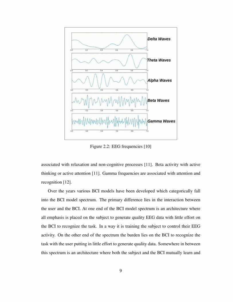
EEG activity is broadly divided into five frequency bands. The boundaries are flexi-

ble but do not vary much from 0.5-4 Hz (delta), 5-8 Hz (theta), 9-12 Hz (alpha), 13-30

Hz (beta) and above 30 Hz (gamma) frequencies. Refer to Figure 2.2 for EEG frequency

bands. The EEG frequencies and their associated activities are the delta activity is asso-

ciated with deep sleep. Theta activity is associated with hypnagogic imagery, rapid eye

movement (REM), sleep, problem solving, attention and hypnosis [8]. Alpha activity is

8

Delta Waves

Gamma Waves

Beta Waves

Alpha Waves

Theta Waves

Figure 2.2: EEG frequencies [10]

associated with relaxation and non-cognitive processes [11]. Beta activity with active

thinking or active attention [11]. Gamma frequencies are associated with attention and

recognition [12].

Over the years various BCI models have been developed which categorically fall

into the BCI model spectrum. The primary difference lies in the interaction between

the user and the BCI. At one end of the BCI model spectrum is an architecture where

all emphasis is placed on the subject to generate quality EEG data with little effort on

the BCI to recognize the task. In a way it is training the subject to control their EEG

activity. On the other end of the spectrum the burden lies on the BCI to recognize the

task with the user putting in little effort to generate quality data. Somewhere in between

this spectrum is an architecture where both the subject and the BCI mutually learn and

9

evolve together. This is achieved when the BCI gives feedback to the user regarding the

quality of EEG data generated [9]. Some BCI architectures also use the error related

negativity (ERN) signals, a type of ERP, which are used along with the EEG to aid in

identification of the subject’s true intentions [13].

10

Chapter 3

Methods

This chapter provides details on the brain-computer interface model. Section 3.1

presents the BCI architecture and the flow of control in this BCI model. Section 3.2

describes the experimental setup and procedures followed in the lab when collecting

EEG data, Section 3.3 gives details of the dataset used in the experiments, Section 3.4

explains the Welch periodogram approach to estimate the power spectral densities from

raw EEG data. Section 3.5 outlines the theory and math in the incremental QDA clas-

sifier algorithm. Section 3.6 evaluates how close the estimated parameters are to the

computed ones. Section 3.7 details on feature selection and the associated preprocess-

ing.

3.1 Brain Computer Interface Architecture

Our brain-computer interface model is geared towards an online approach where timely,

reliable response is of paramount importance. We adopt a non-invasive method to gather

brain electrical activity from the scalp electrodes. The subject is instructed to imagine

performing different tasks. The EEG data, typically in microvolts, is amplified then

converted to digital signals before being processed. The BCI architecture used in this

project is outlined in Figure 3.1.

In the offline mode EEG data samples are divided into train, validation and test par-

11

Feature Selection

Power Spectral Density(PSD)Estimates

Classifier

BCIEEG data samples accumulated over half second intervals

time t1Train PSD

Selected Features

EEG Data

time t2Validate PSD

time t3Test PSD

Figure 3.1: The Brain Computer Interface architecture

titions. Within each partition the samples are collected over half second windows to

estimate the power spectral densities. Power spectral density (PSD) gives the distribu-

tion of average power with respect to the frequencies in the EEG signal. The estimated

PSD’s are binned and treated as individual features within each channel. At time t1

the incremental classifier is trained on these features and the feature selector also ranks

these features. At time t2 the ranked features are evaluated on the validation partition to

determine the bounds on the number of features that help in recognizing the tasks. At

time t3 all features within the selected bounds are used on the test partition to evaluate

the performance.

12

3.2 EEG Data

In our non-invasive approach the subject wears an electrode cap. The electrodes on

the cap are placed as per the 10-20 system, refer to Figure 3.2. The electrodes on the

right hemisphere are even numbered and to the left are odd numbered. The letters on

the electrodes correspond to the lobes as explained in Chapter 2. In addition to the

Frontal, Temporal, Parietal and Occipital lobes, two regions the pre-Frontal (a region

in the frontal lobe) and Central (a region in between the frontal and parietal lobes) are

included. Scalp recordings of neuronal activity in the brain allow measurement of poten-

tial changes over time in the basic electric circuit conducting between the signal (active)

electrodes and reference electrodes [14]. In our setup the reference electrodes, A1 and

A2, are placed on the left and right ear (preauricular points), respectively. Not shown in

Figure 3.2 is the ground electrode which lies in the center of the Fp1, Fp2, FZ triangle

which also pertains to our setup. We used a Mindset [15] EEG recorder to collect data.

A conductive gel is applied to bridge the gap between the scalp and the electrodes.

Impedance at each scalp-electrode contact is adjusted to be less then 5 kilo-ohms in order

to lower signal distortions (equipment dependent). This is done by twirling a wooden

stick around in each channel until the impedances begin to drop covering all channels

repeatedly. Subjects are instructed to perform imagination of actual tasks with a cue. We

used the CEBL software [17] in which the order of tasks are randomly determined. The

visual cues for each task appear for a specific time period interspersed with idle periods.

The EEG signals recorded from the scalp are amplified, digitized and preprocessed for

artifacts. Common artifacts include eye movement, muscle movement, electric motors,

electric lights, etc. While standard lab procedures help eliminate most artifacts, some

artifacts like eye blinks are inevitable. The CEBL software is equipped with a maximum

noise fraction (MNF) filter to filter out the high and low frequencies [2]. Refer to Figure

3.3 for sample EEG data from 19 channels over a five second interval. Eye blink artifacts

13

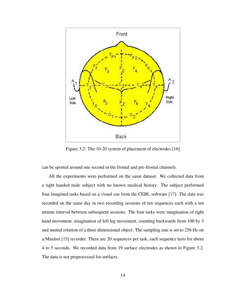
Figure 3.2: The 10-20 system of placement of electrodes [16]

can be spotted around one second in the frontal and pre-frontal channels.

All the experiments were performed on the same dataset. We collected data from

a right handed male subject with no known medical history. The subject performed

four imagined tasks based on a visual cue from the CEBL software [17]. The data was

recorded on the same day in two recording sessions of ten sequences each with a ten

minute interval between subsequent sessions. The four tasks were imagination of right

hand movement, imagination of left leg movement, counting backwards from 100 by 3

and mental rotation of a three dimensional object. The sampling rate is set to 256 Hz on

a Mindset [15] recorder. There are 20 sequences per task, each sequence lasts for about

4 to 5 seconds. We recorded data from 19 surface electrodes as shown in Figure 3.2.

The data is not preprocessed for artifacts.

14

Figure 3.3: Sample EEG data from 19 channels

3.3 Power Spectral Density Estimation

The areas of activation in the brain vary with the tasks (classes) as do the associated

EEG frequencies. For instance bodily movement causes the central and parietal lobe to

generate EEG between 12 Hz (alpha) and 30 Hz (beta). Refer to Figure 2.2 for EEG

frequencies. The power of any signal is defined as the energy per unit time of a signal.

Hence the average power at the scalp electrodes along the direction of the firing neu-

rons will be relatively high when compared to the power at the electrodes farther away

from the line of firing neurons. The PSD’s estimated from raw EEG data closely model

15

the underlying brain frequencies and also improve the classification accuracy [18, 19].

The power spectral density is an estimate of the signal’s power falling within frequency

ranges. To estimate the PSD’s we will need to transform the time domain EEG data into

frequency representations. The occurrence of the frequency components is independent

of where in time this component appears. Therefore PSD estimates of stationary time

signals is straightforward but in the case of EEG it is further complicated as the nonsta-

tionary nature of the human brain generates nonstationary EEG signals [20]. In order

to represent the EEG signals in the frequency domain we would like to assume that the

EEG signals are stationary over a short period of time. Valid assumptions tend to vary

between 0.5 to a few seconds [21].

Two important parameters in estimating the power spectral densities are the upper

and lower bound on the frequencies and how to group the frequencies. Several stud-

ies band pass filtered the frequency components between 6-30 Hz for imagery tasks.

Pfurtscheller, et al., talks about three imagery tasks for patients with actual spinal cord

injury; the frequencies were band pass filtered between 8-30 Hz [22]. Bin, et al., and

Pfurtscheller, et al., band pass filtered between 6-30 Hz and 9-28 Hz, respectively, which

covers both mu and beta rhythm for right and left hand imagery tasks [23, 24]. To group

frequency components into bins we would like to know the active frequencies given

the tasks. From the literature, Wolpaw, et al., showed that alpha (8-13Hz) and/or beta

rhythm amplitudes could serve as effective inputs for a BCI to distinguish a movement

or motor imagery task [25, 26]. Rescher and Rappelsberger performed data reduction of

the spectra into five frequency bands as follows theta (4-7.5 Hz), alpha 1 (8-10 Hz), al-

pha 2 (10.5-12.5 Hz), beta 1 (13-18 Hz), beta 2 (18.5-24 Hz) [27]. Tanaka, et al., groups

the frequencies in pairs (i.e., 6-7 Hz, 8-9 Hz) essentially a 2Hz resolution [19]. From

pilot experiments with our dataset grouping the frequencies into 2 Hz bins increased

the complexity by increasing the number of features and additionally our tasks did not

16

require this small a resolution in the sense we were expecting more changes at the alpha,

beta frequency ranges. This led us to group the frequency components roughly based on

the EEG frequency bands. Clearly this is another search problem that was not intended

to be addressed as part of this thesis. We leave this for future work. One representation

that works well for experiment I is frequency components that are band pass filtered

between 6-24 Hz which covers the ranges for both tasks. The frequency components are

grouped into five bins 6-7 Hz (theta), 8-10 Hz (alpha 1), 11-12 Hz (alpha 2), 13-20 Hz

(beta 1) and 21-24 Hz (beta 2).

We use the Welch periodogram approach to estimate the PSD’s (refer to the Welch-

PSDEstimates pseudo code below). The WelchPSDEstimates() function takes as argu-

ments the raw EEG data, the number of channels and the number of bins the frequency

components will be grouped into. In addition the window type is set to a default Hanning

window; the window size parameter specifies the time period over which the stationary

property of the EEG is assumed to hold; the increment parameter (in percent) specifies

by how many samples the window will need to shift. This last parameter could also be

viewed as what percentage of the signal from the previous time window should be used

to compute the frequency components in the current time window.

17

WELCHPSDESTIMATES(EEGdata, Channel, Bins)

1 Window ← Hanning2 WindowSize← (No.ofsamplesPerHalfSecond)/2

// WindowSize: EEG data accumulated over half second intervals by 23 Increment← WindowSize/4

// Increment: 75% Overlap, 25% Increment between two adjacent windows4 NFFT ← Nyquistfrequency

// NFFT : Number of frequency components5 for i← 1 to Channel6 do FrequencyComponents← stft(EEGdata(Channeli),Window,7 WindowSize, Increment,NFFT )8 AvgFrequencyComponents← Average(FrequencyComponents)9 PSD ← 20 x log10(AvgFrequencyComponents/NFFT )

10 PSDBins← append(PSDBins,Divide(PSD,Bins)11 return PSDBins

Figure 3.4: Sliding Hanning window over half second of EEG data

Figure 3.4 shows several Hanning windows over half second of EEG data from PZ

channel. For this sample window the PSD estimation parameters are No. of sam-

ples=128, Window=Hanning, WindowSize=64 samples, Increment=16 samples. The

Five Hanning windows correspond to samples 1-64, 16-80, 32-96, 48-112 and 64-128.

18

0 20 40 60 80 100 120

−6

0−

40

−2

00

Task=Right hand, channel=C3

Frequency(Hz)

Pow

er/

Fre

qu

en

cy(d

B/H

z)

0 20 40 60 80 100 120

−6

0−

40

−2

00

Task=Left foot, channel=CZ

Frequency(Hz)

Pow

er/

Fre

qu

en

cy(d

B/H

z)

Figure 3.5: Sample PSD estimates for a Right hand (right) and Left foot (left) tasks

The number of frequency components is set to the Nyquist frequency (half the Sampling

rate, 128 Hz). The window size, increment percent and the number of frequency com-

ponents are experiment specific. A wider window accommodates more samples and,

therefore results in a finer resolution of the estimated PSD’s; on the other hand a wider

overlap percentage (smaller increment percentage) causes more windows to slide across

and minimizes total variance giving a better estimate of the PSD’s. This is an important

trade off in the Welch approach. In our experiments we have set the window size to be

half the number of samples per second (i.e., we assumed the EEG is stationary over half

second intervals) and increment to be 25% of the size of the window. The Short Time

Fourier Transform(stft) function [28] determines the frequency content of local sections

(Hanning window worth of data) of a signal. From a half second of EEG data five PSD’s

19

are estimated corresponding to the five Hanning windows (refer to line 6 in the pseudo

code). An average of these five PSD’s result in a sample PSD. The sample PSD’s are

further grouped into frequency bins roughly based on the EEG frequency bands. Sample

PSD estimates for an imagined right hand and left foot movements are shown in Figure

3.5. The dotted lines are the PSD estimates from five windows; the solid black line is

the average over five windows. It can be seen that for a bodily movement task the power

is distributed between 10 Hz to 30 Hz.

3.4 Incremental QDA Algorithm

Quadratic Discriminant Analysis [29] assumes that samples within each class are nor-

mally distributed. Figure 3.6 shows sample Quantile-Quantile (QQ) plots on PSD es-

timates for Fp1 and T4 channels. A 45◦ line implies that the data is perfectly normal.

From offline tests we verified that most channel PSD estimates are near normal. To

classify a sample the QDA classifier computes the probability of that sample belonging

to each class and makes a decision based on the class with the maximum probability.

Using the probability of occurrence of a sample P (x) and the probability of a sample

belonging to a class k, P (C = k), we can define P (C = k, x) and P (x,C = k) using

the product rule as

P (C = k, x) = P (C = k|x)P (x), (3.1)

P (x,C = k) = P (x|C = k)P (C = k) (3.2)

(3.1) and (3.2) represent the same joint probability hence by equating the right sides of

(3.1) and (3.2) gives

P (C = k|x)P (x) = P (x|C = k)P (C = k) (3.3)

20

●

●●

●

●

●

●

●

●

●

●

●

●

●

●

●●

●

●

●

●●

●

●

●

●

●

●●

●

●

●

●

●

●

●

●●

●

●

●

●

●

●

●●

●

●

●

●

●

●

●

●●●●●

●

●

●

●

●

●

●●

●

●

●●

●

●●

●●●

●

●

●●

●

●

●

●

●

●

●

●

●

●

●

●

●

●

●

●

●

●

●

●

●

●

●●

●

●

●

●●

●

●

●●

●

●●●

●

●

●

●

●

●

●

●

●

−2 −1 0 1 2

−1

5−

10

−5

05

10

15

Channel FP1 6−7Hz

Theoretical Quantiles

Sa

mp

le Q

ua

ntile

s

●

●

●

●

●

●●

●

●

●

●

●

●

●

●

●

●

●

●

●

●●

●

●

●

●

●

●●

●●

●

●

●

●

●

●

●

●●

●

●

●

●

●●

●●

●

●

●●

●

●

●

●

●

●

●

●

●

●

●

●

●●

●

●

●●●

●

●

●

●●

●

●

●

●

●

●

●

●

●

●

●

●

●

●

●

●

●

●

●

●

●

●

●

●

●

●

●

●

●

●

●

●

●

●

●

●

●

●

●

●

●

●●

●

●●

●

●

●

●

−2 −1 0 1 2

−1

5−

10

−5

05

10

15

Channel FP1 8−10Hz

Theoretical Quantiles

Sa

mp

le Q

ua

ntile

s

●

●

●

●

●

●

●

●

●

●

●

●

●

●

●

●

●●

●

●●●

●

●

●

●●

●●

●

●

●

●

●

●

●

●

●

●

●

●

●

●

●●

●

●

●

●

●●

●

●

●

●

●

●

●

●

●

●

●

●

●

●

●

●

●

●

●

●

●

●

●

●●

●●

●

●

●

●

●

●

●

●

●

●

●

●

●

●

●

●

●

●

●

●●

●

●

●

●

●

●

●

●

●

●

●

●

●

●

●●

●

●●

●●

●

●●

●

●

●

−2 −1 0 1 2

−1

5−

10

−5

05

10

15

Channel FP1 11−12Hz

Theoretical Quantiles

Sa

mp

le Q

ua

ntile

s

●

●

●

●●

●●

●

●

●●

●

●

●

●

●

●

●

●

●

●

●

●

●●

●

●

●●

●

●

●

●

●

●

●

●●

●

●

●

●

●●

●

●

●

●●

●

●

●

●

●

●

●

●

●

●

●●

●

●

●

●

●●

●

●

●

●

●

●

●

●

●

●

●

●

●●

●

●

●●●

●●

●●

●

●

●

●

●●

●

●

●

●

●

●●

●

●●

●

●

●

●

●

●

●

●

●

●●●

●

●

●

●

●

●

●

●

−2 −1 0 1 2

−1

0−

50

51

0

Channel FP1 13−20Hz

Theoretical Quantiles

Sa

mp

le Q

ua

ntile

s

●

●

●

●

●●●

●

●

●

●

●●

●

●

●●●

●

●

●

●

●

●

●

●

●

●

●

●

●

●

●

●●

●

●

●

●●

●

●

●

●

●

●●

●

●●

●

●

●

●

●

●

●

●

●

●

●

●

●

●

●

●●

●

●

●

●

●

●

●

●

●●

●●

●

●

●

●

●●

●

●

●

●

●

●

●

●●

●

●

●

●

●

●●

●●

●

●

●

●

●

●

●

●

●

●

●

●

●

●

●

●

●

●

●

●

●

●

●

−2 −1 0 1 2

−1

5−

10

−5

0

Channel FP1 21−24Hz

Theoretical Quantiles

Sa

mp

le Q

ua

ntile

s

●

●●

●

●

●

●●

●

●

●

●●

●

●

●

●●

●

●●

●

●

●

●

●

●

●

●

●

●

●

●

●

●

●

●

●

●●

●

●

●

●

●

●

●

●

●

●

●

●

●●

●

●●●●

●

●

●

●●

●●

●●

●

●●

●

●

●●

●

●

●

●●●

●

●

●●

●

●

●

●

●

●

●

●

●

●

●

●

●

●

●

●

●

●●

●

●

●

●

●

●●

●●

●

●●

●

●●

●

●

●

●

●

●

●

−2 −1 0 1 2

−1

5−

10

−5

05

10

15

Channel T4 6−7Hz

Theoretical Quantiles

Sa

mp

le Q

ua

ntile

s

●

●

●

●●

●●

●

●

●

●

●●

●

●

●●

●

●

●

●●

●

●

●

●●

●

●

●

●

●

●

●●

●

●

●

●

●

●

●

●

●

●

●

●●

●

●

●

●●

●

●●●

●

●

●

●

●

●

●

●●

●

●

●●

●

●●

●

●

●

●

●

●●

●

●

●

●●●

●

●

●

●●

●

●

●

●

●●

●

●

●

●

●●

●●

●

●

●●

●

●

●

●

●

●

●

●

●

●

●

●

●

●

●

●●

−2 −1 0 1 2

−1

5−

10

−5

05

10

15

Channel T4 8−10Hz

Theoretical Quantiles

Sa

mp

le Q

ua

ntile

s

●

●

●

●

●

●

●

●

●

●

●●

●

●

●

●

●●

●

●

●

●

●

●

●

●

●

●

●●

●

●●

●

●

●

●●

●

●

●●

●

●

●

●

●

●

●

●

●

●

●

●

●

●●

●

●

●

●

●

●

●

●

●

●

●

●●

●

●●

●

●●

●

●

●

●●

●

●

●●

●

●

●

●

●

●

●

●

●

●

●

●

●

●●

●

●●

●

●

●

●

●

●

●

●

●●

●

●

●

●

●

●

●●

●●

●

●

●

−2 −1 0 1 2

−2

0−

15

−1

0−

50

51

01

5

Channel T4 11−12Hz

Theoretical Quantiles

Sa

mp

le Q

ua

ntile

s

●

●

●

●

●

●

●

●

●

●●

●

●

●

●

●

●

●

●

●

●●

●

●

●

●●

●

●●

●

●●

●

●

●

●

●

●●

●

●

●

●

●

●

●

●

●

●

●●●

●

●

●

●

●

●

●

●

●

●

●●

●

●●

●

●

●●●

●

●

●●

●

●

●

●

●●

●

●

●

●●

●

●

●

●

●

●

●

●

●

●

●●

●

●

●

●

●

●

●

●

●●

●

●

●

●

●

●

●

●

●

●

●

●

●

●

●

●

−2 −1 0 1 2

−1

5−

10

−5

05

10

Channel T4 13−20Hz

Theoretical Quantiles

Sa

mp

le Q

ua

ntile

s

●

●

●

●

●●

●

●

●

●

●

●●

●

●

●

●

●

●

●●

●

●●

●

●●

●

●

●

●

●

●

●

●

●

●

●●

●

●

●

●

●●

●

●

●

●

●●

●

●

●

●

●

●

●

●

●

●

●

●

●

●

●●

●●

●

●●

●

●

●

●

●●

●

●

●●

●●

●●

●

●

●

●

●

●

●●

●

●

●●

●●

●

●

●

●●●●

●

●

●

●

●●

●

●

●

●

●

●

●

●

●

●

●

●

●

−2 −1 0 1 2

−1

5−

10

−5

0

Channel T4 21−24Hz

Theoretical Quantiles

Sa

mp

le Q

ua

ntile

s

Figure 3.6: Normalcy of PSD estimates. Sample QQ Plots for Fp1 and T4 channelelectrode PSD estimates

The above equation can be rearranged to give Baye’s rule,

P (C = k|x) =P (x|C = k)P (C = k)

P (x)(3.4)

From (3.4) The denominator term P (x) is computed by∑k

l=1 P (x|C = l)P (C = l)

which is the sum of probabilities of a sample belonging to each class over all classes,

P (C = k) is the prior probability of a sample from class k; it is 0.5 for two classes with

uniform number of samples, 0.25 for four classes with uniform number of samples,

etc. P (x|C = k) is the probability of sample x belonging to class k. An important

21

assumption in QDA is that this probability is modelled by a Gaussian distribution whose

probability density function is given by,

P (x|C = k) =1

2πp2 |Σk|

12

e−12

(x−µk)T Σ−1k (x−µk), (3.5)

where p is the dimension of the data sample, µk and Σk are the mean and covariance

parameters of class k, respectively. To classify a data sample x to belong to class k, we

pick the maximum probability P (x|C = k), it is equivalent to picking the log(P (x|C =

k)),

log(P (C = k|x)) = log

(P (x|C = k)P (C = k)

P (x)

),

log(P (C = k|x)) = log(P (x|C = k)) + log(P (C = k))

− log(P (x)) (3.6)

Replacing the P (x|C = k) in (3.6) by its probability density function gives

log(P (C = k|x)) = log

(1

2πp2 |Σk|

12

e−12

(x−µk)T Σ−1k (x−µk)

)+ log(P (C = k))− log(P (x)) (3.7)

The right side of (3.7) simplifies to

log(P (C = k|x)) = −p2

log(2π)− 1

2log |Σk| −

1

2(x− µk)TΣ−1

k (x− µk)

+ log(P (C = k))− log(P (x)) (3.8)

In a two class problem sample x is said to belong to the class 1 if

log(P (C = 1|x)) > log(P (C = 2|x)) (3.9)

22

The general form of (3.9) is given by

arg maxk

[log(P (C = k|x))] (3.10)

The corresponding general form of a discriminant function for class k is given by

δk(x) = −1

2log |Σk| −

1

2(x− µk)TΣ−1

k (x− µk) + log(P (C = k)) (3.11)

The negative log of the determinant of the covariance matrix can be expressed as the

log of the determinant of the inverse covariance matrix [30]. From (3.11) replacing

− log |Σk| by log |Σ−1k | gives

δk(x) =1

2log |Σ−1

k | −1

2(x− µk)TΣ−1

k (x− µk) + log(P (C = k)) (3.12)

Hence the mean and inverse covariance matrix are the only parameters that are needed

to determine the probability of a sample belonging to class k. In an incremental QDA

algorithm we are dealing with data samples as they arrive. Hence when the xthl sample

arrives, assuming µk,(1:l−1) represents the mean up until xthl−1 sample, the mean can be

updated as,

µk,(1:l) =(µk,(1:l−1)(l − 1)) + xl

l(3.13)

The inverse covariance matrix can also be updated an incremental fashion. This is our

modification of Berge, et al., nonincremental method [30]. We represent the inverse

covariance matrix by Cholesky Decomposition as

Σ−1k = LTkDkLk, (3.14)

where Lk is a lower triangle matrix and Dk is a diagonal matrix for class k. To estimate

the inverse covariance matrix we will need to estimate the L and D matrices for kth

23

class using Nk training samples. From (3.12) replacing the inverse covariance matrix

with the modified Cholesky decomposition results in

Nk∑i=1

log(P (C = k|x)) =

Nk∑i=1

[1

2log |LTkDkLk| −

1

2(xi − µk)TLTkDkLk(xi − µk)

]

+

Nk∑i=1

[log(P (C = k))] , (3.15)

where Nk is the number of samples in class k and xi is the ith sample in the kth class.

Further Lk can be expressed as I − Bk, where Bk is the lower triangular matrix with

zeros on the principle diagonal and I is the identity matrix. This gives

Nk∑i=1

log(P (C = k|x)) =

Nk∑i=1

[1

2log |(I −Bk)

TDk(I −Bk)|]

−Nk∑i=1

[1

2(xi − µk)T (I −Bk)

TDk(I −Bk)(xi − µk)]

+

Nk∑i=1

[log(P (C = k))] (3.16)

The determinant of I − Bk is 1 by definition hence the first term in (3.16) simplifies to

log |Dk|. Representing the mean subtracted ith sample in the kth class i.e., (xi − µk) by

Vk,i; the log-likelihood of (3.16) with respect to (Bk, Dk) becomes proportional [30] to

Nk∑i=1

log(P (C = k|x)) =

Nk∑i=1

[1

2log |Dk| −

1

2(((I −Bk)

TVk,i)TDk(I −Bk)

TVk,i)

]

+

Nk∑i=1

[log(P (C = k))] (3.17)

Rearranging (3.17) results in

Nk∑i=1

log(P (C = k|x)) =

Nk∑i=1

[1

2

p∑r=1

log dk,r

]

24

−Nk∑i=1

[1

2

p∑r=1

(Vk,i,r −BT

k,r,1:(r−1)Vk,i,1:(r−1)

)2dk,r

]

−Nk∑i=1

[1

2log(P (C = k))

], (3.18)

where

• p is the number of features of a data sample also it is the number of rows/columns

in the inverse covariance matrix,

• dk,r is the rth diagonal entry (same row-column intercept) in the Dk matrix,

• Vk,i,1:(r−1) is rth row comprising of 1 to r-1 column entries in the kth class (V is

the mean subtracted sample (xi − µk)), and

• Bk,r,1:(r−1) is rth row comprising of 1 to r-1 column entries in the kth class (Lower

triangular matrix excluding the diagonal entries).

Differentiating (3.18) with respect to Bk,r,1:(r−1) and dk,r to maximize the likelihood

of Bk,r,1:(r−1) and dk,r and equating it to zero along with some rearranging results in

estimates of Bk and dk,r

Bk,r,1:(r−1) =Vk,i,rV

Tk,i,1:(r−1)

Vk,i,1:(r−1)V Tk,i,1:(r−1)

, (3.19)

dk,r =Nk − 1

[Vk,i,r −BTk,r,1:(r−1)Vk,i,1:(r−1)]2

(3.20)

For Nk samples from kth class, the corresponding B and d matrices can be updated as,

Bk,r,1:(r−1) =

∑Nk

i=1 Vk,i,rVTk,i,1:(r−1)∑Nk

i=1 Vk,i,1:(r−1)VTk,i,1:(r−1)

, (3.21)

dk,r =Nk − 1∑Nk

i=1[Vk,i,r −BTk,r,1:(r−1)Vk,i,1:(r−1)]2

(3.22)

25

Using (3.21) and (3.22) the complete lower triangular matrix is estimated as,

ESTIMATEINVERSECOVMATRIX(sampleki)

1 for m← 1 to rows // rows is the number of rows in the inverse covariance matrix2 do for n← 1 to m −13 do Update Bk,m,n

4 Update Dk,m,m

5 return Bk, Dk

Figure 3.7: The Inverse Covariance matrix for a small 5 feature dataset

Line 3 in the EstimateInverseCovMatrix pseudo code, corresponding to (3.21), can be

viewed as updating the lower triangular matrix (entries 1 through 10) in Figure 3.7 and

line 4 can be viewed as updating the diagonal entries (letters A through E), correspond-

ing to (3.22). Notice that the B matrix will need to be updated before being used in the

D matrix computation. In case all samples were accumulated and the inverse covariance

matrix is estimated, then the estimated inverse covariance matrix would be same as the

computed inverse covariance matrix, subject to the N or N − 1 scaling.

3.5 Divergence between Computed and Estimated pa-rameter distributions

We attempted to quantify how far the estimated parameters are from the computed pa-

rameters. We treated the computed parameters as modeling one distribution and the in-

26

100 105 110 115 120 125

010

000

2000

030

000

4000

0

Kullback−Liebler Divergence

Training Samples

KL

(nat

s)

Right handLeft footArithmeticVisual spinning

(a)

100 105 110 115 120 125

8688

9092

9496

9810

0

Computed vs Estimated parameters performance (Train fraction)

Samples

Cla

ssifi

catio

n ac

cura

cy in

%

● ● ● ● ● ● ● ● ● ● ● ● ● ● ● ● ● ● ● ● ● ● ● ● ● ●

● BatchIncremental

(b)

Figure 3.8: Kullback-Leibler divergence for all four tasks (left) and the associated per-formance on a four task problem (right)

crementally estimated parameters modeling another. The Kullback-Leibler divergence

gives the relative entropy or divergence between an unknown distribution p(x) and an

approximating or model distribution q(x) [29]. It is an asymmetrical quantity. The

divergence is in nat units. The general form of Kullback-Leibler divergence [29] is,

DKL(p||q) = −∫p(x) ln

(q(x)

p(x)

)dx

For two multivariate distributions Nc(µc,Σ−1c ) and Ne(µe,Σ

−1e ) the closed form of

Kullback-Leibler divergence [31] is given by,

DKL(N(µc,Σ−1c )||N(µe,Σ

−1e )) =

1

2

(log

(|Σ−1

c ||Σ−1

e |

)+ trace(Σ−1

e Σc)

)+

1

2

((µc − µe)TΣ−1

e (µc − µe)−N),(3.23)

where µc and Σ−1c are the computed mean and inverse covariance parameters, µe and

Σ−1e are the incrementally estimated mean and inverse covariance parameters, N is the

number of features/attributes in the distributions. Equation (3.23) uses the inverse co-

variance parameter consistent with the parameters estimated in this project; to use the

27

covariance parameter (3.23) will need to be modified accordingly. We used the kl.div()

[32] function in R to compute the KL divergence as samples are added incrementally.

Figure 3.8(a) shows the KL divergence for the computed and estimated parameter dis-

tributions for all four tasks from the sample dataset. Along the x-axis are the training

samples (from train sequences 1-13 only ∼ 125 samples per task) starting from 100

samples. On the y-axis is the KL divergence in nats. We can observe that the divergence

drops steadily as training samples are added one at a time. The final divergence, when

all samples are added, for the four tasks vary between 50 and 70 nats. Using all twenty

sequences from the dataset (∼ 190 samples per task) resulted in final divergences vary-

ing between 15 and 25 nats. We hypothesize as more training samples are added this

divergence will approach zero. The associated performance of the incremental classifier

on the training fraction (trained and tested on the same fraction) on a four task prob-

lem is shown in Figure 3.8(b). We see that as samples are added the incremental QDA

performance gradually approaches batch QDA performance.

3.6 Feature Selection

Feature selection is primarily performed to select relevant and informative features [33].

Feature selection approaches are roughly categorized into Predictor, Filter and Wrapper

methods [33]. Filters rank features based on the training samples filtering out features

that are irrelevant. In the BCI applications we perform feature selection to improve

performance, use the selected features to understand the underlying brain activity and

lastly reduce the number of features thereby the number of parameters to be estimated.

In EEG frequency domain the features are the power spectral densities organized into

frequency bins in each channel. For instance organizing the PSD’s into five bins results

in 95 (19 channels × 5 bins each) features.

28

3.6.1 The Relief Algorithm

The Relief [34] algorithm is a filter based feature selector. It is time-efficient and com-

putationally less expensive. It takes one parameter, the number of iterations, to rank

features. This parameter is experiment specific as it depends on the number of sam-

ples, quality of EEG data, sampling rate and tasks (overlapping/non-overlapping) to be

classified.

The Relief algorithm works by randomly selecting a sample from the training set, find-

ing a nearest hit (sample closest in Euclidean distance from the same class) and near-

est miss (sample closest in Euclidean distance from a different class) [34]. Individual

weights are associated with each feature. Using the nearest hit and nearest miss the

weights are updated by a fraction of a diff factor. This diff factor is computed as,

diff(feature, S1, S2) =|value(feature, S1)− value(feature, S2)|

max(feature)−min(feature),

where S1 is the randomly chosen sample and S2 is the nearest hit/miss, respectively.

The intuition behind Relief is that the features that help recognize the nearest hit are

not so interesting hence decrease their weights and the features that help recognize the

nearest miss are the desirable ones hence increase their weights. This process is repeated

for a set number of iterations which is also the only parameter to this algorithm. After

completion of all iterations sort the updated weights and choose all features with positive

weights. The pseudo code for Relief algorithm is below,

29

RELIEF(features, iterations, Traindata)

1 W [1 : features ]← 0 // Weight vector of length features2 for i← 1 to iterations3 do Randomly select a sample Ri from Traindata4 Hi ← nearesthit(Ri, T raindata)

// Hi: Same class as the random sample Ri

5 Mi ← nearestmiss(Ri, T raindata)// Mi: Different class from the random sample Ri

6 for k ← 1 to features7 do W [k ]← W [k]− diff(k,Ri, Hi)/iterations+8 diff(k,Ri,Mi)/iterations9 return W

Note: The Relief algorithm presented above is for a two class problem. Relief can be

extended to multiple classes [34].

3.6.2 Preprocessing

Prior to feature selection the associated preprocessing will need to performed. We begin

with the QDA discriminant function

δk(x) =1

2log |Σ−1

k | −1

2(x− µk)TΣ−1

k (x− µk) + logP (C = k)

Ideally we would like the feature selector to rank the features in the inverse covariance

matrix that in a way correspond to the product (x − µk)T (x − µk) from the equation

above. Hence we perform some preprocessing to ready the data for feature selection.

Each entry in the inverse covariance matrix corresponds to the interaction between, for

instance, feature a and feature b. We would like Relief to rank this interaction between

pairs of features over individual features. So taking into consideration the interaction

between all possible pairs of N individual features results in N2 features. From this N2

features only N × (N + 1)/2 features are unique since the upper triangular matrix is a

mirror image of the lower triangular matrix. The preprocessing will first require each

feature to be mean subtracted before taking the product. Refer to the Compute pseudo

code below,

30

COMPUTE(features, PSDSamples)

1 for i← 1 to features//features is the number of rows/columns in the inverse covariance matrix

2 do feature1 ← PSDSamples(ithfeature)3 mean1 ← mean(feature1)4 for j ← i to features5 do feature2 ← PSDSamples(jthfeature)6 mean2 ← mean(feature2)7 datareturn ← append[datareturn, ((feature1 −mean1)8 x (feature2 −mean2))]9 featuresupdated ← featuresupdated + 1

10 return datareturn, featuresupdated

This process is repeated for all entries in the lower triangular matrix (upper triangu-

lar matrix is a mirror image of the lower triangular matrix) of the inverse covariance

matrix. The diagonal entries are mean subtracted and squared. The featuresupdated

and datareturn (line 9) are fed as features and Traindata, respectively, to the Relief()

function above. This will drastically blow up the number of features but it gives better

control over feature selection. For instance EEG samples from 19 channels organized

into 5 frequency bins results in a total of 95 features. Further these 95 features are mean

subtracted and multiplied to get (95× 94 / 2) 4465 features which Relief ranks. The top

ranking features are added in a forward selection manner (which implies the lower and

upper triangular matrix entries are set to their respective estimates while low ranking

feature entries are set to zero). By default all diagonal entries are set to their estimates

irrespective of their ranks as this will ensure that the determinant of the inverse covari-

ance matrix exists. The number of Relief iterations is bounded by the number of samples

in the training partition. We have tested the number of iterations to vary between 50% to

90% of the total number of samples (in training partition). By estimating the PSD’s the

total number of samples shrink (128 raw EEG samples translate into one PSD sample)

hence it does not make a significant difference in terms of execution time when the iter-

ations vary between 50% to 90%. The complexity of the task and the ease with which

31

a subject can perform the task will dictate how many iterations Relief will need to pick

the most significant features. In our experiments we have fixed the number of iterations

to 90% of the total number of samples which roughly translates to 226 iterations.

32

Chapter 4

Results

This chapter presents the results from two experiments. From the previous chapter Sec-

tion 3.3 gives the technical details of the data set used in both experiments. Sections 3.4

and 3.7 gives the parameter settings for the power spectral density estimation and the

Relief feature selection.

4.1 Experiment I

In experiment I we evaluate the performance of the proposed BCI model on a two task

problem. The two chosen tasks are imagination of right hand movement and visual

spinning of a three dimensional object.

In the first task the subject was trying to imagine holding a ball, thrown at him,

with his right hand palm facing upwards. This is a motor imagery task that can be

performed in two ways; one, kinesthetic imagery (KI) where the subject imagines per-

forming the task; two, visual imagery (VI) in which the subject visualizes performing

the task. Doyon, et al., reports that KI and VI mediate separate neural systems, which

contribute differently during processes of motor learning and neurological rehabilitation

[35]. Numerous studies have also shown that areas of the brain overlap in motor imagery

(KI) and motor executing tasks (actual movement) and that these areas are not gener-

ally active during visual imagery [36]. Regarding regions of the brain that are active in

33

motor imagery tasks, altered activation has been reported in parietal and premotor areas

during movement imagination [37]. Both areas have also been associated with men-

tal representation of movement [38]. Pfurtscheller, et al., suggests that motor imagery

activates primary sensorimotor cortex (S1 area) [39]. There is conflicting evidence re-

garding the involvement of primary motor cortex (M1 area) [40]. As far as frequencies

are concerned, actual movement tasks are associated with suppression of alpha waves

and exhibition of strong beta waves [41].

In the second task the subject was visualizing a laptop computer spinning around.

The mental rotation is a visual imagery task. There is a lot of overlap in functions and

representations between visual imagery and visual perception [42, 43]. Among others

the visual rotation task is affected by

• the view of the object: canonical or non canonical views cause different regions

of activation in the brain [43];

• dimensionality of the object: two dimensional object rotation has higher EEG

frequency power when compared to three dimensional object rotation [44];

• subject gender accounts for changes during the mental rotation task [27];

• visual imagery arises from interaction between a host of sub processes [36].

The frequencies of the visual spinning task are spread over theta, alpha and beta fre-

quency ranges [27]. Whether imagination of these tasks will trigger activity in the same

frequencies is questionable.

These two tasks were chosen from the original four task experiment since they in-

volve two distinct regions of activation in the brain. In theory the right hand movement

task activates regions of the brain in the left central and left frontal lobes (contralateral

to the hand). The visual spinning task activates the primary visual cortex in the occipital

34

lobe. Whether imagination of these tasks activates similar regions of the brain is subject

to argument. Berthoz, et al., gives counter evidence that transformation of mental im-

ages are in part guided by motor processes even in the case of objects rather than body

parts [45]. In view of this evidence the theory that these two tasks activating different

regions of the brain does not hold. Nevertheless good recognition rates by the BCI on

a two task problem would lead us to some insight into the number of features selected,

what channel-frequency components are highly ranked and the interaction between these

features.

In the BCI offline mode we performed the following steps. First, the dataset is

partitioned into train, validation and test.Then, the BCI is trained on the train partition

and also rank the features are ranked on the same. Next the features are added in a

forward selection manner on the validation partition to identify the peak performance

and the associated set of top features that caused the peak performance. Finally the set

of top ranked features are used on the test partition to evaluate the performance.

Figure 4.1 is a performance plot of the BCI model when averaged over multiple runs

since our feature selection (i.e., Relief) approach incorporates an element of randomness

in the way of selection of samples. Also the results were stable and the trends captured

better when averaged over multiple runs. From pilot experiments the trends observed

were stable over ten iterations or so. Along the x-axis are the features added ten at a

time in a forward selection manner as ranked by Relief on the train partition. We use

the classification accuracy as a performance metric i.e., given a PSD sample the task it

is associated with to by the BCI model is checked against its original target task. The

number of correctly recognized samples are plotted as a percentage of the total number

of samples along the y-axis. The following paragraphs explain each part of the figure,

The points: All plots are averaged over ten iterations. The gray, thick black and solid

black lines correspond to the performances of incremental QDA (using estimated pa-

35

0 100 200 300 400

5060

7080

9010

0

Subject−II TR: 13 VL: 3 TS: 4 Classes: 1 − 4 steps: 10 Relief iter: 226

Features(stepped up by 10 )

Cla

ssifi

catio

n A

ccur

acy(

%)

TrainValidateTest

Diagonals onlyOnlineBatch

Figure 4.1: Experiment I performance plot

rameters) on train, validation and test partitions, respectively. The closely associated

dotted lines correspond to the batch QDA performances (parameters are computed) on

the same three partitions. From the twenty sequences that make up the data set, 13 se-

quences (65%) went into training and ranking the features, 3 sequences (15%) went into

validating the ranked features and 4 sequences (20%) went into testing the performance.

All sequences are ordered by time in the sense the train sequences were recorded first,

followed by the validation and finally the test set. Since the partitions, hence the PSD

samples, are the same for incremental and batch mode performing feature selection in

each mode is the same as performing Relief twice in any one mode. Since our results

are an average over ten iterations we performed feature selection only once in the incre-

36

mental mode. The top ranking features from the incremental mode are also added in a

forward selection manner in the batch mode. The plots reveal that batch and incremen-

tal QDA performances are consistent. Observe that the incremental QDA plots tend to

converge with the batch QDA plots for all three partitions when all features are added

(extreme right) to the inverse covariance matrix.

The horizontal lines: The three dashed lines from top down correspond to BCI perfor-

mance with only the diagonal entries for the test, train and validation partitions, respec-

tively. Recall that our feature selector ranks the features in the lower triangular matrix

of the inverse covariance matrix. In the forward selection approach we start with a di-

agonal inverse covariance matrix and subsequently add ten features at a time. Hence

the dashed line corresponds to the diagonal inverse covariance matrix with no features

added. Essentially it is the inverse covariance matrix with variances only.

The vertical lines: The vertical lines correspond to the peaks in the validation set in the

ten iterations. Although we would like to mention that a different partition of the train,

validation and test would generate different plots.

From Figure 4.1 it can be observed that the validation and test partitions follow sim-

ilar trends. On the other hand the train partition follows a different trend following the

addition of 200 features. This trend will need to be further investigated; we speculate

that it is data dependent as with other datasets different trends were observable. Start-

ing with the diagonal inverse covariance matrix the test performance (solid black line)

vibrates around the first thirty features, rises steadily from 30-80 features and peaks

around 80-90 features then it begins to decline sharply until 250 features. Between 250

to 280 features the performances show a small bump following which they reach the

lowest point. When all features are added to the inverse covariance matrix the inverse

covariance matrices in the batch and incremental approach are essentially the same,

subject to computation or estimation, but the performances still vary because the latter

37

Frequency domain heat map of 1 to 1500 Relief selected features

Frequency bins Hz

Ch

an

ne

ls

6 − 7 8 − 10 11 − 12 13 − 20 21 − 24

FP1

F3

C3

P3

O1

F7

T3

T5

FZ

FP2

F4

C4

P4

O2

F8

T4

T6

CZ

PZ

1

1

2

3

4

5

6

7

7

7

8

9

10

10

11

11

11

12

12

13

13

14

15

16

16

16

17

18

18

18

19

19

20

21

22

22

22

23

23

24

24

25

25

26

26

26

27

28

28

29

30

30

30

31

32 33

34

35

36

36

37

37

38

39

39

40

41

41

42

42

43

44

44

44

44

45

45

46

46

47

47

47

48

48

48

49

49

50

50

51

51

51

51

Figure 4.2: Experiment I 1 to 1500 features heat map

is estimated and the former is computed. Table 4.1 shows the mean performance of

the proposed BCI for experiment I over ten iterations on the test partition. The three

38

Table 4.1: Comparison of performances on test partition for experiment I

Diagonals With Withoutonly Feature Feature

Selection SelectionBatch QDA 67.20% 69.53% 65.01%Incremental QDA 71.88% 73.75% 57.81%

columns correspond to the sparsity of the inverse covariance matrix. The first column

corresponds to the performance only when the diagonal entries are added in the inverse

covariance matrix. The second column corresponds to peak performance when adding

ten features at a time in a forward selection manner and the last column corresponds to a

completely filled inverse covariance matrix. The test partition’s mean performance and

standard deviation with feature selection is 73.75% ± 7.39%. Excluding the two outlier

performances gives a 77%. Note that even though the average performance peak from

the plot is around 84.53%± 1.15% all ten iterations (vertical lines) do not coincide with

the peak hence the difference.

Along with the performance we are also interested in the top features ranked by Re-

lief and added in the forward selection manner which caused the performances to spike

around 80-90 features on an average. Figure 4.2 is a heat map of the top 150 features

ranked in the train partition. A dark shaded box corresponds to a higher rank. Note

that we are adding ten features at a time hence 150 features translates to 1500 (150 x

10) features. Along the x-axis are the frequency bins and along y-axis are the channel

electrodes. Recall when a feature is added essentially we are setting its inverse covari-

ance matrix entry to be non zero. An inverse covariance matrix entry is the interaction

between channel a at bin b with channel c at bin d. For example Fp1 6-7 Hz interacts

with F4 21-24 Hz. This causes the corresponding Fp1 6-7 Hz and F4 21-24 Hz heat

map entry to be incremented by one. In this manner the top 1500 features are tracked

39

Frequency domain heat map of 400 to 1300 Relief selected features

Frequency bins Hz

Ch

an

ne

ls

6 − 7 8 − 10 11 − 12 13 − 20 21 − 24

FP1

F3

C3

P3

O1

F7

T3

T5

FZ

FP2

F4

C4

P4

O2

F8

T4

T6

CZ

PZ

1

1

2

2

3

4

4

5

5

6

7

8

9

10

10

10

11

11

12

12

13

13

14

14

15

15

16

16

16

16

17

17

17

17

17

18

18

18

19

19 20

20

20

21

21

21

21

22

23

23

23

24

24

2526

27

27

27

28 28

28

28

29

30

30 31

32

32

33

33

34

34

35

35

35

35

35

35

36

36

36 36

36

36

37

38

38

38

38

38

38

38

Figure 4.3: Experiment I 400 to 1300 features heat map

over all ten iterations and an average is plotted in Figure 4.2. To get a sense for the

contributing features, P4 21-24 Hz which ranks 1 translates to 2.69% (approximately

40

in 807 instances P4 21-24 Hz is paired with another feature) and T4 21-24 Hz which

ranks 51 translates to 0.06% of the total occurrences over ten iterations. Our hypothesis

on selection of channel electrodes given the tasks are the electrodes spread over the left

central, left frontal and occipital lobes. Relief ranked in order the channels P4, F4, C3,

T4, PZ, T6, F3, F8, Fp1, etc. Other than C3 and F3 there is some inconsistency on

the ranked channels as they are spread over the parietal, right frontal and right temporal

lobes. One simple explanation is the convoluted nature of the brain and neuron firing

properties that electrodes around the central (P4, F4, T4, PZ, F3) and occipital (P4, PZ,

T6) lobes are picking up more signals then the ones actually above them. In total 14

features (including ties) rank among the top ten of which eleven lie in the theta (6-7

Hz) range and three lie in the beta 2 (21-24 Hz) range. Within the top 20 only eight

features lie between 8-20 Hz. This led us to believe that the heat map which represents

the top 1500 features include features that cause the dip in the performance and is not

very specific. Hence we narrowed down our heat map representation to the features that

actually caused the spike in the validation and test partitions.

The top 900 features ranked between 400th to 1300th added features, centered

around the spike, were further analyzed in Figure 4.3. From this heat map among the

top ranked channels in order are F4, P3, F3, PZ, T3, T4, FZ, CZ, T5, C3, P4, C4, etc

among which F4, F3 and P3 are contributing two bins each. It can also be seen that

this heat map projects a different set of channels as top ranked when compared to the

previous heat map. Eleven of the top ten features (including ties) lie in the 6-7 Hz theta

bin and four of the top ten features lie in the beta 2 range. Also there is a lot of activity

in the 8-20 Hz band, eighteen of the top 20 features lie in this range when compared

to eight in the previous heat map. This suggests that more alpha and beta 1 features

causes an increase in performance. In all of the ten iterations we find the right hand task

dominating the visual imagery task in terms of recognition rates. This may be because

41

the features selected aid in recognizing the right hand task over the visual spinning task.

Examining these channels more closely we find channels are being represented from the

contralateral side, ipsilateral side and along the line which divides the two hemispheres.

We, along with Lee, et al., [46] claim that it is difficult to find significant contralateral

characteristics in motor imagery tasks.

0 10 20 30 40 50 60

−60

−40

−20

020

F3

Frequency (Hz)

dB/H

z

0 10 20 30 40 50 60

−40

−20

020

F4

Frequency (Hz)

dB/H

z

Figure 4.4: Experiment I PSD’s of F3 and F4 electrodes for the right hand task on thetrain partition

We speculate that more ipsilateral channel electrodes are chosen as event-related

synchronization (ERS) is present in the ipsilateral side when imagining a right hand

task. Increase in rhythmic activity or synchrony (reflected in the appearance of a spec-

tral peak) due to internally or externally paced events is event-related synchronization

(ERS) and the decrease is event-related desynchronization (ERD) [47, 48]. ERD has

been reported to be a characteristics of voluntary muscle movement [49]. Several stud-

ies claim that in motor imagery tasks there is dominating EEG activity in the ipsilateral

side then the contralateral sighting ERS and ERD phenomenon [49, 50]. Pfurtscheller,

et al., reports something very similar that in a motor imagery task a contralateral ERD

42

dominates an ipsilateral ERS on no feedback sessions, at the onset of the visual cue,

following feedback the ipsilateral ERS becomes apparent [48]. Beisteiner, et al., also

reports widespread DC potential over the contralateral and ipsilateral sides for motor

imagery tasks [51]. Spatial patterns on imagery tasks exhibit relative increase in EEG

variance focused on the ipsilateral side and ERD in the contralateral primary sensori-

motor area [52]. Kamousi, et al., adopts an inverse problem approach to classify motor

imagery tasks using source reconstruction. They claim that during motor imagery a de-

crease in synchrony of the underlying neuronal population causes a decrease of power in

the alpha rhythm in the contralateral side and subsequently stronger activity is reported

on the ipsilateral side [53].

Again these results are based on studies that used single trial EEG in which ERD

and ERS components can be clearly identified. In our experiment the subject repeatedly

performed all tasks following visual cues at one sitting. Based on these findings we

speculate that a right hand imagery task could cause the contralateral channels to have

smaller spectral peaks, resulting in low power when compared to the channels in the

ipsilateral side. The variance in EEG activity in those channels causes Relief to pick

those channels over the others. Figure 4.4 shows the estimated PSD’s for right hand

task on the F3 (contralateral) and F4 (ipsilateral) channels from the training partition

which are both ranked highly by Relief. It can be observed that F3’s peak is shifted yet

tightly coupled around 20 Hz when compared to F4 which shows a lot of variance in

activity around 10 Hz. In addition to channels on the ipsilateral side being chosen more

often we also probed into why the theta bins are chosen more often than the other bins.

Theta oscillations are related to episodic memory process responsible for orientation in

space and time [54]. Increase in theta activity is reported during retention and working

memory tasks and motor imagery is associated with working memory [55, 56]. From

Figure 4.4 notice there is also a lot of variance in the lower frequencies (1-10 Hz). We

43

believe this is due to the half second sliding Hanning window placed over a complete

sequence of EEG data. So there could be instances in which the window is breaking up

a right hand task over two subsequent PSD estimates or maybe even one windows worth

of samples (128 samples) is not enough to capture a snapshot of a complete right hand

task which the subject performs repeatedly.

Figure 4.5: Experiment I F4 at 6-7 Hz (left) and F4 at 21-24 Hz (right)

From the heat map presented above we are interested in which channels the top

channels are frequently paired with. Among the top ten features F4, F3 and P3 have two

bins each in the 6-7 Hz and 21-24 Hz, respectively. Figure 4.5 is a snapshot of the F4

electrode at the two frequency bins: 6-7 Hz (left) and 21-24 Hz (right). Each interaction

is represented by a line. The target electrode frequency bin determines the line style, viz.

6-7 Hz by bold(black), 8-10 Hz by bold (gray), 11-12 Hz by solid, 13-20 Hz by dashed

and 21-24 Hz by dotted. There are instances where more than one line exists between

channels; this implies that the source electrode interacts with more than one bin at the

target electrode. A pair of lines exist only if they occur in nine or more of the ten runs

per experiment. F4 at 6-7 Hz (left) is more sparsely connected then F4 at 21-24 Hz

(right), consistent with the ranks. F4 at 6-7 Hz is highly concentrated within the F3-O1

44

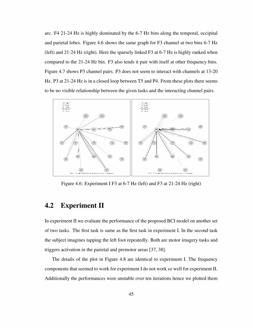
arc. F4 21-24 Hz is highly dominated by the 6-7 Hz bins along the temporal, occipital

and parietal lobes. Figure 4.6 shows the same graph for F3 channel at two bins 6-7 Hz

(left) and 21-24 Hz (right). Here the sparsely linked F3 at 6-7 Hz is highly ranked when

compared to the 21-24 Hz bin. F3 also tends it pair with itself at other frequency bins.

Figure 4.7 shows P3 channel pairs. P3 does not seem to interact with channels at 13-20

Hz. P3 at 21-24 Hz is in a closed loop between T5 and P4. From these plots there seems

to be no visible relationship between the given tasks and the interacting channel pairs.

Figure 4.6: Experiment I F3 at 6-7 Hz (left) and F3 at 21-24 Hz (right)

4.2 Experiment II

In experiment II we evaluate the performance of the proposed BCI model on another set

of two tasks. The first task is same as the first task in experiment I. In the second task

the subject imagines tapping the left foot repeatedly. Both are motor imagery tasks and

triggers activation in the parietal and premotor areas [37, 38].

The details of the plot in Figure 4.8 are identical to experiment I. The frequency

components that seemed to work for experiment I do not work so well for experiment II.

Additionally the performances were unstable over ten iterations hence we plotted them

45

Figure 4.7: Experiment I P3 at 6-7 Hz (left) and P3 at 21-24 Hz (right)

0 100 200 300 400

4050

6070

8090

100

Subject−II TR: 13 VL: 3 TS: 4 Classes: 1 − 2 steps: 10 Relief iter: 226

Features(stepped up by 10 )

Cla

ssifi

catio

n A

ccur

acy(

%)

TrainValidateTest

Diagonals onlyOnlineBatch

Figure 4.8: Experiment II performance plot

46

Table 4.2: Comparison of performances on Test partition for experiment II

Diagonals With Withoutonly Feature Feature

Selection SelectionBatch QDA 56.25% 56.01% 40.62%Incremental QDA 54.69% 56.72% 40.62%

over 20 iterations. First, over twenty iterations the peak performance of the validation

set is spread non uniformly between 20 and 220 features. Additionally the validation

partition peaks at two instances along the feature space which causes the peak test per-

formances to be non uniformly spread out between these two instances. Table 4.2 shows

the mean performance of the proposed BCI for experiment II over twenty iterations on

the test partition. The mean test performance and standard deviation over all twenty

iterations is 56.72% ± 7.41% while actual test performance (where the test partition

actually peaks) is at 67.26% ± 2.23%.

We plotted the heat map for top ranked features centered on the test partition bump

between 500th to 1100th added features. Refer to Figure 4.9. The top 10 features have

several ties and include all the channels but Fp1. Observe that the test and validation

partitions now follow different trends when compared to experiment I. Hence the heat

map on the test bump is projecting the set of features that in a way is directly contributing

to the poor performance. On the other hand the heat map of the features between 2000

and 2600 which cause a spike in the validation set is shown in Figure 4.10. We do see a

lot of alpha, beta 1 and beta 2 bins ranked highly in this experiment. We speculate that if

test had a similar set of features like validation then the trends would synchronize. From

this heat map we probed F3 and F4 channels for possible ERS and ERD characteristics

but none were clearly visible.

The reasons for poor performance of the BCI on experiment II could also be the close

47

Frequency domain heat map of 500 to 1100 Relief selected features

Frequency bins Hz

Ch

an

ne

ls

6 − 7 8 − 10 11 − 12 13 − 20 21 − 24

FP1

F3

C3

P3

O1

F7

T3

T5

FZ

FP2

F4

C4

P4

O2

F8

T4

T6

CZ

PZ

1

1

2

2

2

3

4

5

5

5

5

5

6

6

6

7

8

9

9

9

9

9

10

10 10

11

11

11

11

11

12

12

13

13

13

13

13

13

14

14

14 14

14

15

15

15

1516

16

16

16

17

17

17

17

18

18

18

18

18

19

19

20

20

20

20

20

20

21

21

21

21

22

23

23

24 24

24

24

24

25

25

25

25

25

2627

27

27

27

Figure 4.9: Experiment II 500 to 1100 features heat map

proximity of regions of activation in the two tasks. Additionally the cut off frequencies

and grouping them into five bins may be ineffective. Also the poor performance is due

48

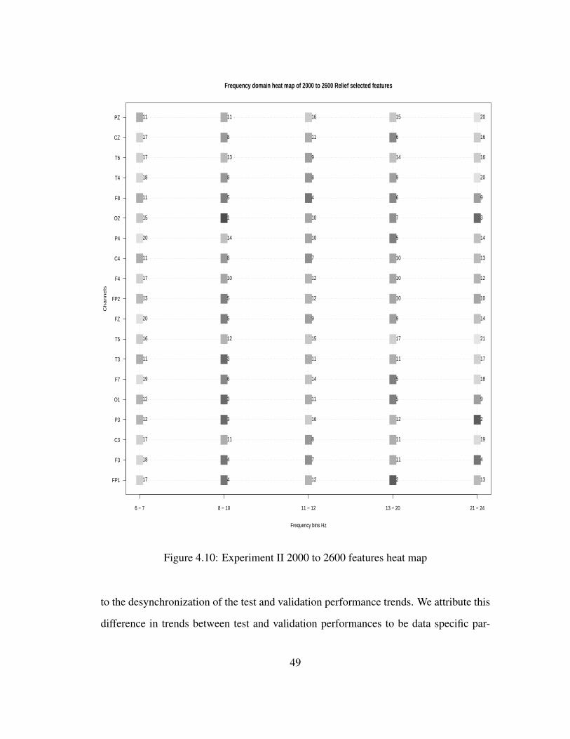
Frequency domain heat map of 2000 to 2600 Relief selected features

Frequency bins Hz

Ch

an

ne

ls

6 − 7 8 − 10 11 − 12 13 − 20 21 − 24

FP1

F3

C3

P3

O1

F7

T3

T5

FZ

FP2

F4

C4

P4

O2

F8

T4

T6

CZ

PZ

1

2

23

3

3

3

4

4

4

4

5

5

5

5

5

5

6

6

6

7

7

7

8

8

8

8

8

9

9

9

9

9

9

10

10

10

10

10

10

10

11

11

11

11

11

11

11

11

11

11

11

11

12

12

12

12

12

12

12

12

13

13

13

13

14

14

14

14

14

15

15

15

16

16

16

16

16

17

17

17

17

17

17

17

18

18

1819

19

20

20

20

20

21

Figure 4.10: Experiment II 2000 to 2600 features heat map

to the desynchronization of the test and validation performance trends. We attribute this

difference in trends between test and validation performances to be data specific par-

49

ticularly the partition of the train, validation and test sets. From pilot experiments, a

different partition gives better performance and compatible trends but this in turn vio-

lates the time constraints placed on the partitions; from the EEG data sequences the first

set of sequences goes into training, intermediate set goes into validating and the last set

goes into testing, as this ordering replicates a real world problem.

4.3 Comparison of Execution Time

We compared the execution time taken to compute the inverse covariance matrix be-

tween batch, the Berge, et al., algorithm [30] and our incremental approach. In the batch

approach we used the cov() and solve() [57] R functions to compute the covariance and

inverse covariance, respectively. The Berge, et al., [30] algorithm is written in R and

computes the inverse covariance matrix using all data samples but looping through each

row in the inverse covariance matrix once and updating the corresponding columns. In

essence it computes the B and D matrices similar to our incremental approach but for

all samples simultaneously using matrix computations. In the incremental approach we

loop over all samples and for each sample update all rows in the B and D matrices

following which we compute the inverse covariance matrix. Hence for sample k from

a N sample dataset such that 1 < k < N we have an estimated inverse covariance

matrix up until the kth sample. These three approaches cannot be directly compared

for execution time as the first two approaches use matrix computation. Hence for the

incremental approach we have plotted the average execution time over all samples. We

chose to plot the average time since in an online BCI application when the inverse co-

variance matrix up until sample k already exists we will only need to update the inverse

covariance matrix for the k+1th sample whereas batch and the Berge, et al., approaches

will need to recompute the inverse covariance matrix for k + 1 samples. Figure 4.11

shows the execution (elapsed) time in seconds over datasets of size 100, 1000, 10000

50

and 100000 samples, respectively. The number of features in each dataset is set to a con-

stant 95 (corresponding to the number of features in our experiments). The data samples

are generated from standard normal distribution. All experiments were performed on a

64 bit Linux system. It took the incremental approach approximately 163 minutes to

compute the inverse covariance matrix for a 100000 sample dataset this translates to an

average of 0.10 seconds per sample. Also in the incremental approach as the number of

samples increased in powers of 10 (i.e. from 100 to 1000) the elapsed time increased

from 21 seconds to 123 seconds. We think the real potential of this incremental approach

can be explored when samples from multiple training sessions are used to only update

the sparse inverse covariance matrix, as determined from the previous training session,

when the other two approaches will need to compute the same using all samples from

all training sessions. We realize this is not an efficient way to compare performances

but nevertheless it gives some insight on the execution time of the approaches.

51

● ● ●●

010

2030

40

Performance time

No. of Samples

Ela

psed

tim

e (s

econ

ds)

● Batch approachBerge, et al, approachIncremental approach

100 1000 10000 100000

Figure 4.11: Comparison of execution time taken to compute the inverse covariancematrix

52

Chapter 5

Conclusion and Future Work

In this project we presented a brain-computer interface model that recognizes one task

from another in a timely manner. We performed two experiments to demonstrate the

strengths and weaknesses of the BCI model. Both experiments followed procedures

and settings akin to real world scenarios. From the performance plots the incremental

and batch approaches are compatible in performance with the added advantage that this

incremental model greatly minimizes the computational complexity by updating the pa-

rameters incrementally. We performed feature selection solely to improve the recogni-

tion rates which would complement the classifier. We find that feature selection greatly

improves the classification accuracies by nearly 16%. Also experiments I and II show

that only 1200 of the 4465 features or a 26.87% of the total features, are required to

achieve a peak performance. In terms of execution time the incremental approach takes

approximately 0.13 seconds, for any given sample, to update the inverse covariance ma-

trix. This should particularly prove useful when data samples from multiple training

sessions are used to train the BCI.

From a neuroscience perspective the information provided by the selected features

does not relate in obvious ways with our current understanding of the underlying brain

activity. This is most likely due to the interaction between the various statistical proce-

dures which fail to capture the big picture. Also the interaction between experimental

53

Table 5.1: Time Embedded lag and skip on a sample dataset

Sample dataset Lag 1 skip 0 Lag 1 skip 1

[,1] [,2] [,3] [,1] [,2] [,3] [,4] [,5] [,6] [,1] [,2] [,3] [,4] [,5] [,6]

1 8.3 70 10.3 1 8.3 70 10.3 8.6 65 10.3 1 8.3 70 10.3 8.8 63 10.22 8.6 65 10.3 2 8.6 65 10.3 8.8 63 10.2 2 8.6 65 10.3 10.5 72 16.43 8.8 63 10.2 3 8.8 63 10.2 10.5 72 16.4 3 8.8 63 10.2 10.7 81 18.84 10.5 72 16.4 4 10.5 72 16.4 10.7 81 18.8 4 10.5 72 16.4 10.8 83 19.75 10.7 81 18.8 5 10.7 81 18.8 10.8 83 19.7 5 10.7 81 18.8 11.0 66 15.66 10.8 83 19.7 6 10.8 83 19.7 11.0 66 15.6 6 10.8 83 19.7 11.0 75 18.27 11.0 66 15.6 7 11.0 66 15.6 11.0 75 18.2 7 11.0 66 15.6 11.1 80 22.68 11.0 75 18.2 8 11.0 75 18.2 11.1 80 22.6 8 11.0 75 18.2 11.2 75 19.99 11.1 80 22.6 9 11.1 80 22.6 11.2 75 19.910 11.2 75 19.9

settings have not been systematically explored in this project. This includes parameters

from power spectral density estimation: window size, window type, individual PSDs

versus averaged PSDs, cut off frequencies and grouping of frequencies into bins; from

Relief the number of iterations. We believe these settings will need to be probed per

subject and/or per task basis and should not be generalized.

One direction of future work is the investigation of EEG signals in the time domain

(i.e., by not estimating the power spectral densities instead using the raw EEG data to

recognize tasks) with and without time embedded lag. In the time domain the incre-

mental QDA’s performance is consistent with batch QDA. But it appears that in both

approaches the top features as ranked by Relief fail to improve performance. As a result

the BCI’s performance is close to and in some cases worse then random performance.

We would like to study in detail the reasons for this poor performance. Within time

domain, time embedded lag uses multiple samples to make a classification decision. A

skip factor determines how many samples are interleaved to make a decision. When

54

skip is zero the samples are adjacent. Refer to Table 5.1 for a time embedded lag and

skip example on a ten sample three attribute dataset. It has been demonstrated that time

embedded lag considerably improves recognition rates in EEG based brain-computer

interface [58]. We performed some preliminary experiments with time embedded lag

with and without skip on the dataset I. It was identified that for right hand and visual

spinning tasks the best lag skip combination is 5-5. Using this lag-skip combination on

the validation set results in a recognition rate of 75.33% without any feature selection.

Another subject for future work would be a more systematic approach to determine the

cut off frequencies and grouping of frequencies into bins in frequency domain. We

would also like to experiment with more datasets to check for consistency in trends and

performance.

55

REFERENCES

[1] J. R. Wolpaw, N. Birbaumer, W. J. Heetderks, D. J. McFarland, P. H. Peckham,G. Schalk, E. Donchin, L. A. Quatrano, C. J. Robinson, and T. M. Vaughan. BrainComputer Interface Technology: A Review of the First International Meeting.IEEE Transactions on Rehabilitation Engineering, 8(2):164–173, 2000.

[2] J. N. Knight. Signal Fraction Analysis and Artifact Removal in EEG. Master’sthesis, Colorado State University, Fort Collins, CO, 2003.

[3] D. J. McFarland, W. A. Sarnacki, T. M. Vaughan, and J. R. Wolpaw. Brain-computer interface (BCI) operation: signal and noise during early training ses-sions. Clinical Neurophysiology, 116(1):56–62, 2005.

[4] A. Kubler, F. Nijboer, J. Mellinger, T. M. Vaughan, H. Pawelzik, G. Schalk, D. J.McFarland, N. Birbaumer, and J. R. Wolpaw. Patients with ALS can use senso-rimotor rhythms to operate a brain-computer interface. Neurology, 64(10):1775–1777, 2005.

[5] J. del R. Millan, J. Mouri no, M. Franze, F. Cincotti, M. Varsta, J. Heikkonen,and F. Babiloni. A Local Neural Classifier for the Recognition of EEG PatternsAssociated to Mental Tasks. IEEE Transactions on Neural Networks, 13(3):678–686, 2002.

[6] A. J. Murias. Biology and Geology Interaction in Humans. http://www.sciencehelpdesk.com.

[7] M. Teplan. Fundamentals of EEG Measurement. Measurement Science Review,2:1–11, 2002.

[8] R. M. Stern, W. J. Ray, and K. S. Quigley. Brain Electroencephalography andImaging. In Psychophysiological Recording, pages 79–105. Oxford UniversityPress, 2000.

[9] J. del R. Millan, P.W. Ferrez, F. Galan, E. Lew, and R. Chavarriaga. Non Inva-sive Brain-Machine Interaction. International Journal of Pattern Recognition andArtificial Intelligence, 20(10):1–13, 2007.

56

[10] Wikipedia. Electroencephalography. http://en.wikipedia.org/wiki/Electroencephalography.

[11] S. Sanei and J. A. Chambers. EEG Signal Processing. Wiley-Interscience, 2007.

[12] O. Jensen, J. Kaiser, and J. P. Lachaux. Human gamma-frequency oscillationsassociated with attention and memory. Trends in Neurosciences, 30(7):317–324,2007.

[13] J. del R. Millan and P.W. Ferrez. Error-related EEG potentials generated duringsimulated brain-computer interaction. IEEE Transactions on Biomedical Engi-neering, 55(3):923–929, 2008.

[14] G. V. Kondraske. Neurophysiological Measurements. In J. Bronzino, editor,Biomedical Engineering and Instrumentation: Basic Concepts and Applications,pages 138–179. PWS Engineering, 1986.

[15] NeuroPulse Systems. Neuropulse Systems LLC. http://www.np-systems.com/.

[16] E. H. Chudler. Neuroscience for Kids. http://faculty.washington.edu/chudler/1020.html.

[17] C. Anderson. CSU EEG Brain-computer interface Lab (CEBL). http://www.cs.colostate.edu/eeg/eegSoftware.html.

[18] F. Galan, M. Nuttin, E. Lew, P.W. Ferrez, G. Vanacker, J. Philips, and J. delR. Millan. A brain-actuated wheelchair: asynchronous and non-invasive brain-computer interfaces for continuous control of robots. Clinical Neurophysiology,119(9):2159–2169, 2008.

[19] K. Tanaka, T. Kurita, F. Meyer, L. Berthouze, and T. Kawabe. Stepwise FeatureSelection by Cross Validation for EEG-based brain computer Interface. In 2006International Joint Conference on Neural Networks, pages 4672–4677, 2006.

[20] A. Y. Kaplan, A. A. Fingelkurts, A. A. Fingelkurts, S. V. Borisov, andB. S. Darkhovsky. Nonstationary nature of the brain activity as revealed byEEG/MEG: Methodological, practical and conceptual challenges. Signal Process-ing, 85(11):2190–2212, 2005.

[21] N. Srinivasan. Cognitive neuroscience of creativity: EEG based approaches. Neu-rocognitive Mechanisms of Creativity: A Toolkit, Methods, 42(2):109–116, 2007.

[22] G. Pfurtscheller, P. Linortner, R. Winkler, G. Korisek, and G. Muller-Putz. Dis-crimination of Motor Imagery-Induced EEG Patterns in Patients with CompleteSpinal Cord Injury. Computational Intelligence and Neuroscience, 2009:publishedonline, 2009.

57

[23] W.Tao, D. Jie, and H. Bin. Classification of motor imagery EEG patterns andtheir topographic representation. In Annual International Conference of the IEEEEngineering in Medicine and Biology Society, volume 2, pages 4359–4362, 2004.

[24] G. Pfurtscheller, C. Neuper, A. Schlogl, and K. Lugger. Separability of EEG sig-nals recorded during right and left motor imagery using adaptive autoregressive pa-rameters. IEEE Transactions on Rehabilitation Engineering, 6(3):316–325, 1998.

[25] D. J. McFarland, L. McCane, L. A. Miner, T. M. Vaughan, and J. R. Wolpaw. EEGmu and beta rhythm topographies with movement imagery and actual movement.Society for Neuroscience Abstracts, page 1277, 1997.

[26] J. R. Wolpaw, D. J. McFarland, G. W. Neat, and C. A. Forneris. An EEG-BasedBrain Computer Interface for Cursor Control. Electroencephalography and clini-cal neurophysiology, 78(3):252–259, 1991.

[27] B. Rescher and P. Rappelsberger. Gender dependent EEG-changes during a mentalrotation task. International Journal of Psychophysiology, 33(3):209–222, 1999.

[28] E. Dimitriadou, K. Hornik, F. Leisch, D. Meyer, and A. Weingessel. R pack-age e1071. http://cran.r-project.org/web/packages/e1071/index.html.

[29] C. M. Bishop. Pattern Recognition and Machine Learning. Springer, 2007.

[30] A. Berge, A. Jensen, and A. S. Solberg. Sparse Inverse Covariance Estimatesfor Hyperspectral Image Classification. IEEE Transactions on Geoscience andRemote Sensing, 45(5):1399–1407, 2007.

[31] W. D. Penny. Kullback-Leibler Divergences of Normal, Gamma, Dirichletand Wishart densities. http://www.fil.ion.ucl.ac.uk/˜wpenny/publications/densities.ps.

[32] P. Simecek. R Package yest. http://cran.r-project.org/web/packages/yest/index.html.

[33] I. Guyon and A. Elisseeff. An Introduction to Feature Extraction. In I. Guyon,S. Gunn, M. Nikravesh, and L. A. Zadeh, editors, Feature Extraction Foundationsand Applications, Series: Studies in Fuzziness and Soft Computing, pages 1–25.Springer, 2006.

[34] M. Robnik-Sikonja and I. Kononenko. Theoretical and Empirical Analysis of Re-liefF and RreliefF. Machine Learning, 53(1-2):23–69, 2003.

[35] A. Guillot, C. Collet, V. A. Nguyen, F. Malouin, C. Richards, and J. Doyon. Brainactivity during visual versus kinesthetic imagery: an fMRI study. Human BrainMapping, 30(7):2157–2172, 2009.

58

[36] G. Ganis, W. L. Thompson, F. Mast, and S. M. Kossyln. The Brains Minds images:The Cognitive Neuroscience of Mental Imagery. In M. S. Gazzaniga, editor, TheCognitive Neurosciences, pages 931–941. The MIT Press, 2004.

[37] S. Lehericy, E. Gerardin, J. B. Poline, S. Meunier, P. F. Van de Moortele, D. LeBihan, and M. Vidailhet. Motor execution and imagination networks in post-strokedystonia. Neuroreport, 15(12):1887–1890, 2004.

[38] E. Gerardin, A. Sirigu, S. Lehericy, J. B. Poline, B. Gaymard, C. Marsault, Y. Agid,and D Le Bihan. Partially overlapping neural networks for real and imagined handmovements. Cerebral Cortex, 10(11):1093–1104, 2000.

[39] G. Pfurtscheller and C. Neuper. Motor imagery activates primary sensorimotorarea in humans. Neuroscience Letters, 239(2-3):65–68, 1997.

[40] C. M. Stinear, W. D. Byblow, M. Steyvers, O. Levin, and S. P. Swinnen. Kines-thetic, but not visual, motor imagery modulates corticomotor excitability. Experi-mental Brain Research, 168(1-2):157–164, 2006.

[41] J. L. Andreassi. Psychophysiology: Human Behavior and Physiological Response.Lawrence Erlbaum, 2000.

[42] G. Ganis, W. L. Thompson, and S. M. Kosslyn. Brain areas underlying visualmental imagery and visual perception:an fMRI study. Cognitive Brain Research,20(2):226–241, 2004.

[43] S. M. Kosslyn, W. L. Thompson, and G. Ganis. The Case for Mental Imagery.Oxford University Press, 2006.

[44] A. R. Nikolaev and A.P. Anokhin. EEG frequency ranges during perception andmental rotation of two-and three-dimensional objects. Biomedical and Life Sci-ences, 28(6):670–677, 1998.

[45] M. Wexler, S. M. Kosslyn, and A. Berthoz. Motor processes in mental rotation.Cognition, 68(1):77–94, 1998.

[46] S. H. Choi and M. Lee. Estimation of Motor Imaginary using fMRI Experimentbased EEG Sensor Location. International Journal of Computational IntelligenceResearch, 3(1):46–49, 2007.

[47] G. Pfurtscheller and F. L. da Silva. EEG Event-Related Desynchronization (ERD)and Event-Related Synchronization (ERS). In E. Niedermeyer and F. L. da Silva,editors, Electroencephalography: Basic Principles, Clinical Applications, and Re-lated Fields, pages 1003–1016. Lippincott Williams & Wilkins, 2004.

59

[48] G. Pfurtscheller, R. Scherer, and C. Neuper. EEG-based Brain Computer Inter-face. In R. Parasuraman and M. Rizzo, editors, Neuroergonomics: The Brain atWork (Oxford Series in Human-Technology Interaction), pages 315–328. OxfordUniversity Press, 2006.

[49] G. Pfurtscheller and C. Neuper. Motor Imagery activates primary sensorimotorarea in humans. Neuroscience Letters, 239(2-3):65–68, 1997.

[50] L. Qin, L. Ding, and Bin He. Motor imagery classification by means of sourceanalysis for brain computer interface applications. Journal of Neural Engineering,1(3):135–141, 2004.

[51] R. Beisteiner, P. Hollinger, G. Lindinger, W. Lang, and A. Berthoz. Mental rep-resentations of movements. Brain potentials associated with imagination of handmovements. Electroencephalography and Clinical Neurophysiology, 96(6):183–193, 1995.

[52] H. Ramoser, J. M. Gerking, and G. Pfurtscheller. Optimal Spatial Filtering ofSingle Trial EEG During Imagined Hand Movement. IEEE Transactions on Re-habilitation Engineering, 8(4):441–446, 2000.

[53] B. Kamousi, Z. Liu, and B. He. An EEG Inverse Solution based Brain-ComputerInterface. International Society for Bioelectromagnetism, 7(2):Online journal,2005.

[54] D. Popivanov, S. Jivkova, V. Stomonyakov, and G. Nicolova. Effect of independentcomponent analysis on multifractality of EEG during visual-motor task. SignalProcessing, 85(11):2112–2123, 2005.

[55] A. Erfani and A. Erfanian. The Effects of Mental practice and Concentration Skillson EEG Brain Dynamics During Motor Imagery Using Independent ComponentAnalysis. In 26th Annual International Conference of the IEEE EMBS, volume 1,pages 239–242, 2004.

[56] F. Malouin, S. Belleville, C. L. Richards, J. Desrosiers, and J. Doyon. Workingmemory and mental practice outcomes after stroke. Archives of Physical Medicineand Rehabilitation, 85(2):177–183, 2005.

[57] R. A. Becker, J. M. Chambers, and A. R. Wilks. The New S Language: A Pro-gramming Environment for Data Analysis and Graphics. Chapman & Hall, 1988.

[58] A. Sokolov. Analysis of Temporal Structure and Normality in EEG data. Master’sthesis, Colorado State University, Fort Collins, CO, 2007.

60