DEVELOPMENT AND EVALUATION OF A NOVEL NEURAL

NETWORK OF PMSM FOR ELECTRIC VEHICLE

by

HOYUN JAY WON

SHUHUI LI, COMMITTEE CHAIR

YANG KI HONG TIMOTHY HASKEW

HWAN SIK YOON

A THESIS

Submitted in partial fulfillment of the requirements for the degree of Master of Science

in the Department of Electrical and Computer Engineering in the Graduate School of

The University of Alabama

TUSCALOOSA, ALABAMA

2016

Copyright Hoyun Jay Won 2016 ALL RIGHTS RESERVED

ii

ABSTRACT

This thesis investigates an artificial neural network (ANN)-based field-oriented control

(FOC) for a surface-mounted and an interior-mounted permanent magnet synchronous machine

(SPMSM and IPMSM). The ANN was trained by using Levenberg-Marquardt and forward

accumulation through time algorithm.

First, the thesis examines the fundamentals of motor parameters and two aforementioned

vector controls, with training algorithms, in detail. Then, the background and various algorithms

of Maximum Torque per Ampere (MTPA) and flux weakening (FW) control are undertaken

while the following part epitomizes an off-the-shelf component-based electric vehicle (EV)

model that is constructed using MATLAB SimPowerSystems and SimDriveline.

The proposed control is validated in both simulation and hardware experiment and

compared with a PI-based field-oriented control. First, for SPMSM, the results of simulation and

hardware experiment show that the maximum operating speed of the proposed control is

improved by 48% and 3.5% compared to the PI-based control. For IPMSM, the results show that

the proposed control produces less d-axis current than the latter control.

Moreover, the control is implemented and simulated in electric vehicle model, which is

constructed using SimPowerSystems and SimDriveline library in Simulink by the author with

off-the-shelf components. The results show that the proposed controller can be a potential

replacement of the existing control schemes, such as PID, fuzzy logic, or others, and provides

adequate traction control in EV application

iii

DEDICATION

This thesis is dedicated to everyone who helped me and guided me through the process of

creating this document. Among many contributors, such as my family, Dr. Li, and Xingang Fu, I

like to truly give this glory to J. C.

iv

LIST OF ABBREVIATIONS AND SYMBOLS

PMSM Permanent Magnet Synchronous Machine

mmf Magneto-motive Force EMF Electromagnetic-motive Force

( )aaF t

Space vector magneto-motive force in the air gap, where “a” denotes the reference stator a- axis with an angle of 0° while “→” illustrates an instantaneous quantity

je 1 cos sinj

θda Angle between d- and a- axis

( )dsi t

Space vector stator current with the d-axis as the reference axis

, ,a b ci Phase a, b, and c current

s abc dqT

Matrix that changes abc to dqreference frame (Park’s transformation)

s dq abcT

Matrix that changes dq to abc reference frame (inverse Park’s transformation)

Rcoil Coil resistance

Tc Number of turns in the coil

ρ Electrical resistivity [Ω·m]

L Mean turn length [m]

n Number of parallel strands in each conductor

A Cross-sectional area of one strand [m2]

Nc Number of multiple coils per phase

v

Rph Phase resistance

αparallel Parallel paths

ρ0 Electrical resistivity at 20°C

T Temperature

T0 20°C

e Induced voltage

Lg, slot, end Air-gap, stator slot-leakage, and end-turn inductance

Mg, σ Air-gap and leakage mutual inductance

Rs Stator phase resistance

Lsd,sq Stator d- and q-axis inductance

λsd,sq Stator d- and q-axis flux linkage

vsd,sq Stator d- and q-axis voltage

isd,sq Stator d- and q-axis current

Kt Torque constant

λfd Flux linkage constant

Ke Back-emf constant

p Number of pole pairs

ωm Mechanical angular velocity

ωror ωe Electrical angular velocity (ωr = p * ωm)

Jeq Motor inertia

Tem Electromagnetic torque

Tload Load torque

U(·) Utility function

vi

C(·) DP Cost function

ed,q Error function of dq current

sd,q Integrals of the error terms

γ Discount factor

J Jacobian matrix

p Parameter vector

x Estimated measurement vector

δp Minimization function

/C w

Gradient of weight vector

V(·) Error function for pattern

μ Parameter that determines the steepest descent algorithm and Gauss Newton

Epochmax Maximum of Epoch

βde, in Decreasing and increasing factor

μmax Maximum acceptable μ

min/C w

Norm of the minimum acceptable gradient

LM Levenberg-Marquardt

FATT Forward accumulation through time

FOC Field-oriented Control

PI Proportional-Integral

PM Permanent Magnet

RNN Recurrent Neural Network

ANN Artificial Neural Network

NN Neural Network

vii

DP Dynamic Programming

IPMSM Interior mounted PMSM

SPMSM Surface mounted PMSM

PWM Pulse Width Modulation

SPWM Sinusoidal PWM

SVPWM Space Vector PWM

viii

ACKNOWLEDGMENTS

If I was only one to prepare this thesis, I would like to inform that this thesis will not be

done. I like to express my gratitude to my family, colleagues, friends, mentors, and faculty

advisors. Further, the one who gave this topic to research and support was Dr. Shuhui Li,

associate professor and the chairman of this thesis. Without his support and guide, I couldn’t

learn and have the experiences that were provided throughout this thesis. In addition, I would

like to appreciate the support and care from Dr. Xingang Fu, who trained and gave guidelines to

the neural network control. Lastly, I would like to express my appreciation to all faculty

members. They provided the academic material and led me to pursue the Masters.

My family waited two years, even though it would have been one year, to complete this

thesis. When I was depressed that I couldn’t finish this thesis by one year, they encouraged me

by saying “keep it up”.

Among the contributors and supporters, the most support came from J.C.

ix

CONTENTS

ABSTRACT ................................................................................................ ii

DEDICATION ........................................................................................... iii

LIST OF ABBREVIATIONS AND SYMBOLS ...................................... iv

ACKNOWLEDGMENTS ....................................................................... viii

LIST OF TABLES ................................................................................... xiii

LIST OF FIGURES ................................................................................. xiv

CHAPTER 1: INTRODUCTION ................................................................1

1.1 Literature Review.............................................................................2

1.2 Research Motivation ........................................................................5

1.3 Thesis Organization .........................................................................5

CHAPTER 2: MODELING PMSM ............................................................6

2.1 Background Information of PM Motor .............................................6

2.2 PM Motor Parameter.........................................................................7

2.2.1 Resistance ..................................................................................9

2.2.2 Inductance ................................................................................11

2.2.3 Back-EMF Constant, Flux Linkage Constant, and Torque Constant ...................................................................................14

2.2.4 Mechanical Parameters and Number of Poles .........................16

2.3 Park’s Transformation and Inverse Park’s Transformation ............19

2.4 Mathematical PMSM Model...........................................................21

x

2.5 Simulink PMSM Model ..................................................................22

CHAPTER 3: CONVENTIONAL AND NN CONTROL PMSM ............27

3.1 General Overview of FOC ..............................................................27

3.2 Standard PI-based Field-Oriented Vector Control ..........................28

3.2.1 Simulink Model ........................................................................31

3.3 Neural Network Control .................................................................33

3.3.1 Mathematical Model .................................................................34

3.3.2 Training .....................................................................................36

3.3.2.1 Dynamic Programming .......................................................37

3.3.2.2 Levenberg-Marquardt Algorithm ........................................39

3.3.2.3 Forward Accumulation Through Time (FATT) Algorithm ............................................................................41

3.3.2.4 Training Algorithm .............................................................43

3.3.3 Simulink Model ........................................................................45

CHAPTER 4: MTPA AND FLUX WEAKENING...................................47

4.1 General Operation of PMSM ..........................................................48

4.2 MTPA Algorithm ............................................................................52

4.3 Flux Weakening Algorithm ............................................................55

4.3.1 PI-based Control .......................................................................56

4.3.2 Hysteresis Discrete Control ......................................................57

4.3.3 Ferrari’s Method Control ..........................................................57

4.3.4 Constant Voltage Constant Power (CVCP) Control .................58

CHAPTER 5: ELECTRIC VEHICLE MODEL ........................................60

5.1 Driver ..............................................................................................63

xi

5.2 Motor Drive and ESS ......................................................................65

5.2.1 ‘Max torque’ Block ...................................................................66

5.2.2 ‘APP to Reference Torque’ Block ............................................68

5.2.3 ‘Controller’ Block .....................................................................68

5.2.4 ‘Motor and Inverter’ Block .......................................................69

5.2.5 ‘ESS’ Block ..............................................................................72

5.3 Shaft and Differential ......................................................................74

5.4 Tire, Chassis, and Brake .................................................................76

5.4.1 Tire ............................................................................................77

5.4.2 Brake .........................................................................................78

5.4.3 Chassis ......................................................................................79

CHAPTER 6: SIMULATION RESULTS .................................................81

6.1 SPMSM Simulation Result .............................................................81

6.1.1 Motor Parameter and Simulation Setup ....................................81

6.1.2 Results .......................................................................................84

6.2 IPMSM Simulation Result ..............................................................89

6.2.1 Motor Parameter and Simulation Setup ....................................89

6.2.2 Results .......................................................................................90

6.3 Electric Vehicle ...............................................................................93

CHAPTER 7: HARDWARE RESULTS ...................................................97

7.1 Hardware Experiment Component Description ..............................97

7.2 Software Setup ..............................................................................103

7.3 SVPWM ........................................................................................105

xii

7.4 Hardware Setup .............................................................................112

7.5 Results ...........................................................................................113

7.5.1 Acceleration and Deceleration Test ........................................114

7.5.2 Load Torque Variation Test ....................................................116

7.5.3 Flux Weakening Control Test .................................................118

CHAPTER 8: CONCLUSION ................................................................120

8.1 Limitations and Future Work ........................................................122

REFERENCES ........................................................................................123

xiii

LIST OF TABLES

1.1 Types of motor in various vehicles ........................................................1

2.1 Electrical resistivity of copper, aluminum, and silver ...........................9

3.1 Results of DP example .........................................................................39

3.2 FATT algorithm to calculate the Jacobian matrix ...............................43

5.1 Part and Simulink block name for components ...................................62

5.2 EV specifications .................................................................................62

5.3 Descriptions of ESS components .........................................................72

6.1 0.2 kW PMSM parameter in simulation and hardware study ..............82

7.1 Opal-RT OP8660 data acquisition interface pinouts .........................102

7.2 Duration time for each sector .............................................................110

xiv

LIST OF FIGURES

Fig. 1.1 Chart of current publications ..........................................................4

Fig. 2.1 High level a) model of and b) parameters of the PMSM in SimPowerSystems ..........................................................................8

Fig. 2.2 Measuring the stator resistance using digital multimeter .............10

Fig. 2.3 Four-terminal measurement schematic .........................................10

Fig. 2.4 a) Surface mounted magnets, b) Inset rotor magnets, c) Buried tangential magnets, d) Spoke-type magnets, e) V-shape magnets, and f) Multilayer V-shape magnets PM ........................11

Fig. 2.5 Inductance measurement schematic circuit ..................................13

Fig. 2.6 a) Step voltage input across A and B phase and b) switch on/off, current response (green), and step voltage input (purple) ............14

Fig. 2.7 a) Torque and speed curve and b) current and speed curve ..........16

Fig. 2.8 Coast down test .............................................................................18

Fig. 2.9 Back-EMF test ..............................................................................19

Fig. 2.10 Reference frame ..........................................................................20

Fig. 2.11 Overall PMSM block diagram ....................................................23

Fig. 2.12 Block diagram of electrical model ..............................................24

Fig. 2.13 Block diagram of iq,id subsystem ..............................................24

Fig. 2.14 Block diagram of iq subsystem ..................................................25

Fig. 2.15 Block diagram of id subsystem ..................................................25

Fig. 2.16 Block diagram of mechanical model ..........................................26

xv

Fig. 3.1 Overall block diagram of FOC for IPMs ......................................27

Fig. 3.2 Typical output of PI controller .....................................................29

Fig. 3.3 Standard dq field-oriented vector control .....................................29

Fig. 3.4 Overall motor drive schematic (simulation) .................................32

Fig. 3.5 Conventional controller in Simulink ............................................33

Fig. 3.6 PMSM conventional and neural network vector control ..............35

Fig. 3.7 DP example ...................................................................................37

Fig. 3.8 Overall flowchart of training NN controller using LM+FATT algorithm ......................................................................................44

Fig. 3.9 Average DP cost per trajectory time step for training the NN controller ......................................................................................45

Fig. 3.10 Block diagram of the NN controller ...........................................45

Fig. 3.11 Block diagram of the NN current controller ...............................46

Fig. 3.12 Block diagram representation of RNN control ...........................46

Fig. 4.1 Torque versus speed curve of PMSM with other descriptions .....48

Fig. 4.2 a) Torque and speed curve with four different regions and b) Segmentation of operation region for current contour region .49

Fig. 4.3 Ellipse ...........................................................................................51

Fig. 4.4 Voltage and current limit circle with constant torque curve and MTPA for IPMSM .......................................................................51

Fig. 4.5 Adaptive flux weakening control method ....................................56

Fig. 4.6 C-code in Switch block.................................................................56

Fig. 5.1 Overall schematic of the EV .........................................................61

Fig. 5.2 Overall block diagram of the EV ..................................................61

Fig. 5.3 Overall block diagram of the EV in Simulink ..............................61

xvi

Fig. 5.4 Block diagram in Driver block .....................................................63

Fig. 5.5 a) UDDS, b) HWFET, and c) US06 drivecycle ...........................64

Fig. 5.6 Stateflow diagram of the braking shift logic ................................65

Fig. 5.7 Block diagram in Motor Drive block ...........................................66

Fig. 5.8 Overall schematic of motor drive .................................................66

Fig. 5.9 ‘Max torque’ block diagram .........................................................67

Fig. 5.10 ‘Heat index’ block diagram ........................................................68

Fig. 5.11 ‘APP2RefTrq’ block diagram .....................................................68

Fig. 5.12 ‘Controller’ block diagram .........................................................69

Fig. 5.13 Inside view of ‘motor and inverter’ block ..................................70

Fig. 5.14 a) Actual motor and b) specification in graph ............................71

Fig. 5.15 Drawing of PM100DX inverter ..................................................72

Fig. 5.16 Overall block diagram of the ESS ..............................................73

Fig. 5.17 a) Schematic of 1 module and b) overall ESS ............................74

Fig. 5.18 Overall block diagram of ‘Shaft and Differential’ block ...........75

Fig. 5.19 Simulink to PS Torque block diagram .......................................75

Fig. 5.20 Overall diagram of ‘Chassis and Tire’ block ..............................77

Fig. 5.21 Inside view of ‘wheel’ block ......................................................78

Fig. 6.1 Speed traction of SPMSM (simulation)........................................85

Fig. 6.2 ANN d- and q-axis current traction of SPMSM (simulation) ......86

Fig. 6.3 Conventional d- and q-axis current traction of SPMSM (simulation) ..................................................................................86

Fig. 6.4 ANN abc current traction of SPMSM (simulation) ......................87

Fig. 6.5 Conventional abc current traction of SPMSM (simulation) .........87

xvii

Fig. 6.6 ANN normalized amplitude of voltage of SPMSM (simulation) ..................................................................................88

Fig. 6.7 Conventional normalized amplitude of voltage of SPMSM (simulation) ..................................................................................88

Fig. 6.8 Speed traction of IPMSM (simulation) ........................................91

Fig. 6.9 D-and q-axis current traction of IPMSM (simulation) .................91

Fig. 6.10 ANN abc current traction of IPMSM (simulation) .....................92

Fig. 6.11 Conventional abc current traction of IPMSM (simulation) ........92

Fig. 6.12 Normalized amplitude of voltage of IPMSM (simulation) ........93

Fig. 6.13 Speed traction of EV ...................................................................94

Fig. 6.14 Torque traction of EV .................................................................95

Fig. 6.15 D- and q-axis current traction of EV ..........................................95

Fig. 6.16 ANN APP and hydraulic braking traction of EV .......................96

Fig. 6.17 ANN APP and SOC traction of EV ............................................96

Fig. 7.1 Schematic of the hardware experiment ........................................97

Fig. 7.2 Physical wiring of hardware experiment ......................................98

Fig. 7.3 dSPACE CP1103 pinout description ............................................99

Fig. 7.4 Vishay-Hirel MOSFET inverter .................................................100

Fig. 7.5 Lab-volt IGBT inverter ...............................................................100

Fig. 7.6 Lab-volt power supply ................................................................101

Fig. 7.7 Opal-RT OP8660 data acquisition interface ...............................102

Fig. 7.8 DC generator (left) and PMSM motor (right) kit .......................103

Fig. 7.9 Schematic of SVPWM based hardware experiment...................104

Fig. 7.10 Overview of ControlDesk .........................................................105

xviii

Fig. 7.11 SVPWM block and description for hardware experiment) ......106

Fig. 7.12 Basic voltage vectors ................................................................108

Fig. 7.13 Space vector diagram for sector 1, described with a) the duty cycle, b) switching ....................................................................109

Fig. 7.14 Waveform showing sequence of switching states for each sector .......................................................................................111

Fig. 7.15 Calculation of T1/Tp and T2/Tp block .....................................112

Fig. 7.16 Speed traction of SPMSM (hardware)......................................115

Fig. 7.17 Dq-axis current traction of SPMSM (hardware) ......................115

Fig. 7.18 Vm of SPMSM (hardware).......................................................116

Fig. 7.19 Load torque Vm traction of SPMSM .......................................117

Fig. 7.20 a) Conventional and b) ANN speed traction of SPMSM .........118

Fig. 7.21 a) Conventional and b) ANN voltage magnitude of SPMSM ..119

Fig. 7.22 a) Conventional and b) ANN d-axis reference current of SPMSM .....................................................................................119

Fig. 7.23 a) Conventional and b) ANN actual dq current traction of SPMSM .....................................................................................119

1

CHAPTER 1

INTRODUCTION

Among various AC machines, permanent magnet synchronous motors (PMSMs) gained

the most attention due to the following advantages: high torque-inertia ratio, high efficiency,

high power density, and compact structure [1, 2]. These advantages led PMSMs to be utilized in

various applications such as air conditioner, refrigerator, direct-drive washing machines,

automotive electrical power steering, machine tools, traction control, and data storage

applications [3]. Furthermore, with the advent of the hybrid electric vehicle and electric vehicle,

the demand for PMSMs has grown exponentially. Other machines, such as induction motor and

synchronous reluctance motor, also received attention, but due to its high torque density, less

weight, high dynamic performance under load, high efficiency, and the absence of heat, PMSMs

dominated the market [4]. As Table 1.1 suggests, four out of five vehicles are using PMSM in its

application.

Vehicle Type of motor Toyota Prius Permanent magnet AC synchronous motor [5]

Tesla Model S Four pole AC induction motor [6] Hyundai Sonata hybrid Interior permanent magnet synchronous motor [7]

Nissan Leaf EV AC synchronous electric motor [8] Honda Accord hybrid AC synchronous permanent-magnet electric motor [9]

Table 1.1: Types of motor in various vehicles

In DC motor, the stator and rotor can be excited independently. Usually, the value of flux

can be controlled by applying the current through the stator while the torque can be controlled by

manipulating the current through the rotor windings. On the other hand, in AC motor, the stator

2

and rotor cannot be excited independently. Generally, only source that can be controlled is the

stator currents. However, with the advent of Field Oriented Control (FOC), the decoupled control

of torque and flux in AC machines became possible by transforming alternating three-phase

currents into DC two-phase currents. This algorithm not only produces high efficiency in a wide

range of speeds, but also makes motor control easier in both low speed and high speed.

1.1 Literature Review

In general, the current industries use a PI-based field-oriented control to operate PMSMs,

The advantage of the PI controller is its simplicity and ease of understanding. However, recent

studies show that such control strategy is experiencing the following bottlenecks: a) difficulty to

obtain the optimal PI coefficients that satisfy both stability and performance, b) no true

decoupling between torque and flux, and c) limited stability and performance [1, 10]. To

overcome these obstacles, various control schemes were proposed.

Tzann-Shin Lee et al. [1] proposed an adaptive H∞ controller to enhance the stability in

system under parameter perturbations and external disturbances. To accomplish the task, a

quadratic storage function was chosen with a state feedback term to produce a simple adaptive

law for the controller. The study applied periodic step and sinusoidal commands to test its

controller. Although the study proved its effectiveness under the preceding conditions, it did not

show any result when the motor was in high speed or random speeds.

Kamel et al. [11] utilized a fuzzy logic controller with 49 rules to drive the PMSM and

compared the results with the conventional PI-based vector controller. The result showed that the

proposed fuzzy logic controller tracked the speed reference faster and stabilized faster when load

torque disturbance occurred. However, the evaluation was verified only in simulation.

3

Lu et al. [12] employed a self-constructing recurrent fuzzy neural network (SCRFNN) to

control the PMSM online. The proposed SCRFNN was incorporated with two control schemes:

self-constructing fuzzy neural network and recurrent neural network. Even though the proposed

control showed good performance, the validation was only done in simulation. In addition, the

simplified mathematical model of PMSM was used for simulation.

Xia et al. [13] presented a novel direct torque and flux control for matrix converter based

PMSM drive. The study investigated all matrix converter switching states to control input and

output variable. Four switching schemes were based on the tables, which have optimal selections

of switching. Compared with the conventional PI based controller, the matrix converter based

PMSM drive achieved to reduce 30% of the standard deviations of torque and flux and 9% of the

total harmonic distortion. However, even though the result shows improvement, implementing

this technology in industry is difficult because most industries utilize either IGBT or MOSFET

based inverter fed drive.

Khan et al [14] proposed a novel neuro-network-based self-tuned controller for IPMSM

drives. With having the speed error and its change as inputs, the weights, translation, and dilation

of the wavelet functions were altered. Simultaneously, a back propagation training algorithm

continuously manipulated the controller parameter. Additionally, the Lyapunov stability was

used to enhance the system robustness and stability. The controller was validated through both

simulation and hardware and compared with PI-based controller. The author asserted that the

proposed controller produced zero speed overshoot and undershoot and performed better against

load changes than PI-controller. However, only minimal improvement was observed.

J. Moreno et al [15] applied a neural network control in hybrid vehicle energy

management system to minimize the discharge of the batteries. A test vehicle was equipped with

4

two primary energy sources: lead-acid batteries and ultracapacitor bank. The result showed that

the NN control achieved 8.9% increase in range. The experiment was validated in both

simulation and hardware.

Z. Chen et al [16] utilized two NN modules that are trained by dynamic programming to

optimally manage the energy between engine and battery in power-split hybrid electric vehicle.

This control was effective when the trip length and trip duration were known before the trip

starts. The proposed technology was validated only in simulation.

Figure 1.1 shows the chart of the current publications relating to PMSM controls, where

the values in parentheses are referring to the total publications, including conference and journal

papers. As it illustrates, only few papers covered PMSMs in wide speed range and automotive

applications.

Figure 1.1: Chart of current publications

0

20

40

60

80

100

120

140

Fuzzy Logic (294) Neural Network(500)

H∞ Controller (600) Model Predictive(300)

31

50

125

40

5 2 0 00 0 0 0

Experiment Wide Speed+Exp Vehicle+Wide Spd+Exp

5

1.2 Research Motivation

The literature search suggests that there is no research conducted on an artificial neural

network-based vector control for PMSM including both flux weakening control and EV

implementation. Thus, this thesis proposes the neural network vector control for both SPMSM

and IPMSM with flux weakening control. The SPMSM motor drive with the proposed control

will be validated through both simulation and experiment. Further, the IPMSM will be

implemented in EV model that the author has made using the MATLAB tools.

1.3 Thesis Organization

The thesis is organized as follows. Chapter 2 gives the full descriptions of PMSM by

explaining the motor parameters that affect the control while Chapter 3 introduces the

conventional PI-based vector control and proposed neural network vector control with full

descriptions on training algorithm. The next chapter discusses a maximum torque per ampere

(MTPA) control algorithm and flux weakening control, whereas Chapter 5 covers the EV

simulation model that was constructed using SimPowerSystems and SimDriveline. Chapter 6

shows the simulation result of the NN control for SPMSM, IPMSM, and IPMSM in EV

application while Chapter 7 presents the hardware result of SPMSM. Finally, the conclusion of

the thesis is provided in Chapter 8.

6

CHAPTER 2

MODELLING PMSM

Before investigating the controls for PMSMs, this section briefly summarizes the motor

parameters that affect the control. First, a background of PM machines is epitomized, and the

second subsection discusses the fundamentals of the motor parameter, such as stator resistance,

inductances, flux linkages, associated constants, motor inertia, and number of poles. In the final

subsection, the mathematical model and Simulink model of PMSM is covered.

2.1 Background Information of PM motor

Many electrical machine literatures had classified and organized PM machines into

different families to improve understanding of similarities and differences, associated with PM

machines. In this text, the author has chosen to organize the machines according to 1) the

direction of field distribution, 2) configuration of stator winding, and 3) physical structure of

rotor.

In general, depending on the direction of the field distribution, PM machines are divided

into two types. If radial-directed fields are in the airgap, it is called radial-flux PM machine while

if the field in the airgap is axial direction, it is called axial-flux or “pancake” PM machine. In

current EV application, the radial-flux machines are utilized more than the axial-flux machine

because the former machine has easier manufacturing process and more space flexibility than the

latter. Thereby, this thesis chose to investigate the radial-flux machine.

7

Within the radial-flux PM machine, there are two types of stator winding: distributed and

concentrated. A distributed wounded stator winding produces a sinusoidally distributed field in

the air gap while a concentrated stator winding produces a trapezoidal distributed field

distribution. If the stator winding is distributed winding, it is called PMSM or PMAC while if the

stator winding is concentrated winding, it is called brushless DC motor (BLDC). Out of two, the

most commonly used radial-flux machine is PMSM because it is much easier to produce the

sinusoidal waveform than the trapezoidal waveform. Furthermore, FOC can be implemented

only for PMSM because FOC cannot interpret the trapezoidal fields. Thus, in this thesis, the PM

machine that is equipped with distributed stator winding was used.

Lastly, the radial PM machines are divided further by the location of magnets in the rotor.

If magnets are on the surface of the rotor, it is called surface-mounted PM machines (SPMSMs),

whereas interior-mounted PM machines (IPMSMs) has magnets inside the rotor. This context

has investigated both machines because both machines are widely used for various applications.

2.2 PM Motor Parameter

For overall simulation, the PMSM model from MATLAB/ SimPowerSystems is used.

Figure 2.1a shows the high-level PMSM model in MATLAB/SimPowerSystems while Fig. 2.1b

represents the parameters that are necessitated by the model. The main reason for employing this

block is that it not only provides the interface between other components in SimPowerSystems,

but also has easy GUI to be used. As Fig. 2.1b illustrates, the parameters that are required by the

model are 1) stator resistance, 2) armature inductance, 3) flux linkage constant, 4) inertia, and 5)

motor pole pairs.

8

Figure 2.1: High level a) model of, b) parameters of the PMSM in SimPowerSystems

9

2.2.1 Resistance

The primary purpose of the stator is producing the rotating magnetic field in the airgap to

rotate the rotor. In the stator, the rotating magnetic field can be produced by applying the current

through the stator coil. For every coil, there is an intrinsic resistivity associated with it. Table 2.1

shows the intrinsic resistivity of enameled copper, aluminum, and silver [17].

Material Resistivity (Ω·m) at 20 ºC Enameled copper 1.68 x 10-8

Aluminum 2.82 x 10-8 Silver 1.59 x 10-8

Table 2.1: Electrical resistivity of copper, aluminum, and silver

By using the resistivity, the resistance of the coil can be calculated by

R ρ (2-1)

where Rcoil is the electrical resistance of single coil [Ω]; ρ is the electrical resistivity [Ω·m]; l is

the length of the coil [m]; and A is the cross-sectional area of the coil [m2]. Since the stator will

have multiple turns per phase, the phase resistance is

R N ∗ R (2-2)

where Nc is the number of turns.

There are two ways to measure the resistance using either modern multimeter or LCR

meter: two-wire technique and four-terminal resistance measurement. Generally, the latter

method is more accurate than the former method because the latter method excludes the

resistance of the test lead from the actual measurement. Thus, this thesis will elucidate the

instructions of four-terminal resistance measurement.

Usually, the stator winding is connected in an internal “wye” connection, which causes

the neutral point to be hidden in the stator, and thus inaccessible. Thereby, to measure the stator

resistance, two phase resistances have to be measured. Figure 2.2 shows the aforementioned

10

measuring connection while Figure 2.3 illustrates the schematic of four-terminal measurement.

As Fig. 2.2 shows, a positive probe is connected with A-phase while a negative probe with C-

phase. Note that putting the probe is on other phases are allowed.

Figure 2.2: Measuring the stator resistance using digital multimeter

Figure 2.3: Four-terminal measurement schematic

11

2.2.2 Inductance

The synchronous inductance of PMSMs is denoting the inductance of a winding in the

synchronous reference frame. If the reference frame is changed from a stationary reference frame

to a rotating reference frame, the synchronous inductance is divided into two inductances: d- and

q-axis inductance. The d-and q-axis inductance can be found by using these equations.

, 0° (2-3)

, 90° (2-4)

in which L is the synchronous inductance while Ld and Lq denotes the d- and q-axis inductance

[18]. More information about transforming reference frames can be found in Section 2.3.

Generally, the location of magnets determines the d- and q-axis inductances. If PM motor

has its magnets on the surface of the rotor (SPMSM), the inductances of d and q-axis are same

while if the PM motor has its PMs in the rotor (IPMSM), the inductances are different for d and

q-axis. Figure 2.4 represents the configuration of surface and interior mounted PM motors.

Figure 2.4: a) Surface mounted magnets, b) Inset rotor magnets, c) Buried tangential magnets, d)

Spoke-type magnets, e) V-shape magnets, and f) Multilayer V-shape magnets PMSM [19]

12

The inductances affect the performance of the motor as follows [20].

1. The inductive voltage drop absorbs a fraction of the supply. Thus, the base and maximum

speed drops.

2. In sinewave, the inductance affects the power factor. The bigger the inductance is, the

more reactive power has to be produced.

3. It distorts the excitation flux of the magnets, changes the torque constant nonlinearly, and

causes the armature reaction when the stator current is flowing through the conductor.

4. It also hinders the power electronic drives.

5. Lastly, there is possibility of short-circuit fault error.

To measure the d- and q- axis inductances, four equipment are required. They are 1)

DC power supply, 2) oscilloscope, 3) current probes, and 4) voltage probe. First, to measure

the d-axis inductance, the rotor needs to be aligned to Phase A. One can accomplish that by

connecting the positive potential of power supply to Phase A terminal and the negative

potential to Phase B or C terminal. Then, turn on the power supply and increase the voltage

slightly. After alignment, lock the rotor. Then, one needs to connect Phase B and C

terminals to the positive potential while ground Phase A. This connection allows to apply

negative voltage across the circuit. Then, apply a current probe on conductor that connects

Phase A and positive potential. After checking previous connections, turn on the power

supply [21].

In real environment, if the step voltage is applied, it will look like blue line and

purple line in Fig. 2.6a and 2.6b, respectively. The current will behave like green curve in

Fig. 2.6b. Then, one can determine the d-axis inductance by using this equation [21].

13

1 , / (2-5)

where V is the amplitude of the applied voltage and R is the line-to-line resistance. Likewise, the

q-axis inductance can be measured, except the rotor needs to be aligned to q-axis. This can be

done by connecting Phase B to the positive terminal while Phase C to the negative terminal.

Phase A is not used.

Figure 2.5: Inductance measurement schematic circuit

14

Figure 2.6: a) Step voltage input across A and B phase b) switch on/off (yellow), current

response (green), and step voltage input (purple)

2.2.3 Back-EMF Constant, Flux Linkage Constant, and Torque Constant

Back-EMF, torque, and flux linkage constants are important constants for evaluating

machine performance. First, the back-EMF constant describes the behavior of back-EMF with

respect to mechanical speed of the machine. Generally, the units of the back-EMF constant are in

Volts line-to-line (VL-L)/Revolution per Minutes (RPM). Some manufacturers use Volts root

mean square (VRMS)/kRPM. Second, the torque constant describes the output torque per current.

The units of the torque constant are in Nm/ARMS. Again, some manufacturers use Nm/Apeak.

Third, the flux linkage constant describes the flux linkage that is produced by permanent magnet

on or in the rotor. The units of this constant are in Volts·Seconds (V·s). At first glance, these

15

three terms are not interrelated to each other, but they are. These constants can be equated to

each other using proper gains like shown in below equations.

∙/

∙ ∙ (2-6)

∙ ∙ (2-7)

/∙ (2-8)

As illustrated, since all motor constants are correlated to each other, knowing one motor

constant can calculate others without difficulty. Thus, this thesis will mainly cover the

measurement method for back-EMF. However, to give more measuring options to readers, this

thesis will also include the measuring method for torque constant.

First, to measure the back-EMF constant of the machine, an extra motor and an

oscilloscope are needed. Since the primary objective of the extra motor is running the test motor

with constant speed, any kinds of motor can be used. The first step is connecting the auxiliary

and test motor through the mechanical shaft as shown in Fig. 7.8. The next step is rotating the

test motor with certain constant speed. Then, connect positive and negative probe to any phase

terminal while other end of the probe with the oscilloscope. This will measure the peak line-to-

line voltage. The back-EMF constant can be calculated by dividing the measured voltage with

the speed [18].

Second, to measure the torque constant, the only required resources are the motor torque

vs. speed graph and motor current vs. speed graph. Usually, the manufacturer provides these data.

The torque constant of the machine can be calculated by dividing the torque with the current at

specific speed. If the units of the current are in RMS, a peak value can be calculated by

multiplying √2 to the RMS value. Figure 2.7a shows the typical torque and speed curve, whereas

16

Figure 2.7b shows the associated current and speed curve with a).

Figure 2.7: a) Torque and speed curve and b) current and speed curve

2.2.4 Mechanical Parameters and Number of Poles

The concept of mechanical parameters of machines begins with the electrodynamic

equation.

(2-9)

in which Jeq is the inertia of the machine; ωr is the mechanical speed of the motor; Tem is the

electromagnetic torque from the motor; b is the viscous damping coefficient; Jo is the coulomb

friction constant; and Tload is the external load torque. In this equation, there are three mechanical

parameters: inertia, viscous damping coefficient, and coulomb friction constant.

First, the inertia of PM motors determines the performance between the mechanical

stability and acceleration and deceleration. Larger the inertia, better the mechanical stability is,

but lesser acceleration and deceleration performance is. Further, the inertia is proportional to the

size of the machine. Bigger the size, larger the inertia is. Generally, the units of the inertia are in

kg·m2.

17

Second, the viscous damping coefficient describes the energy dissipation due to the

movement of the machine. Usually, it is related with vibration of the machine. The units of this

coefficient are in Nm·second.

Lastly, the coulomb friction constant denotes the shaft static friction. In most cases, the

coulomb friction constant is neglected in calculation and simulation because the impact of the

shaft static friction is minimal. The units are in Nm.

In general, most manufacturers provide these mechanical parameters. However, using

provided values for simulation and experiment may produce inaccurate results because these

parameters are measured when the motor is not connected with other system. Thus, measuring

the mechanical parameters with the complete system is needed for accurate result.

First, to calculate the inertia, determining b and J0 is needed. These values can be

measured by using the method in [21]. After identifying b and Jo, the inertia can be found by

using a method called Coast down test. The test is really simple.

The first step is rotating the test motor to its maximum operating speed. Then, the next

step is disconnecting the power by either unplug the cable or turn off the controller. The rotor

speed will behave as in Figure 2.8. The final step is applying this equation to calculate the inertia.

(2-10)

As it shows, at t= 0.2 sec, the power is off. Then, the motor is spun down to a stop at 0.6 sec.

18

Figure 2.8: Coast down test [21]

The number of poles defines a ratio between electrical and mechanical quantities

(mechanical vs. electrical rotor position/angular speed). Thus, determining the number of poles

in machines is important. Usually, the number of poles is written on the label of the motor.

However, if the manufacturer does not provide this information, one can determine the number

of poles by using back-EMF test that was discussed earlier in section 2.2.3. Figure 2.9 shows the

typical back-EMF vs. time graph. The number of poles can be calculated using this equation.

P (2-11)

19

Figure 2.9: Back-EMF test

2.3 Park’s Transformation and Inverse Park’s Transformation

Park’s transformation triggered the AC machine to gain attentions from the world

because it allowed to control AC machine like controlling DC machine by reducing the three AC

quantities to two DC quantities.

The concept of Park’s transformation begins with Clarke’s transformation, which

converts abc-winding into αβ-quadrature winding.

1 20 2

, whereγ (2-12)

20

As the equation exhibits, the outputs are still time dependent. This can be solved by using Park’s

transformation, which transforms αβ-quadrature winding stationary reference frame into rotating

reference frame.

, where (2-13)

where θda is the angle between the a-axis and d-axis. If Eq. 2-12 and 2-13 are combined, the

resultant equation becomes

(2-14)

where Figure 2.10 illustrates Clarke’s transformation and Park’s transformation graphically.

Lastly, the equation that transforms dq axis to abc winding is called inverse Park’s

transformation.

cos sin

cos sin

cos sin

→

(2-15)

Figure 2.10: Reference frame [22]

21

2.4 Mathematical PMSM Model

The concept of the mathematical PMSM model begins with the stator d- and q-axis

flux linkage equations, which are written as:

(2-16)

where Lsd,sq are the stator d- and q-axis inductances and equal to Lmd,mq + Lls while λfd is the flux

linkage constant of the stator d-axis winding due to flux produced by the magnets in the rotor,

where it is assumed that the d-axis is always aligned with the rotor magnetic axis, which is a-

axis.

In terms of the aforementioned flux linkage equation, the stator winding voltages can be

written as follows.

(2-17)

in which ωe is the electrical angular velocity in electrical rad/s. The electrical angular velocity

can be calculated by multiplying the electromechanical angular velocity, ωmech, with the pole

pairs, p. If Eq. 2-16 and Eq. 2-17 are combined, the equation becomes

0λ (2-18)

where P is the derivative with respect to time. Under a balanced sinusoidal steady state

condition, the terms associated with the time derivative are neglected. Thus, the dq currents

become DC. As a result, Eq. 2-18 in steady state can be rewritten as

0λ (2-19)

The electromagnetic torque for asynchronous and synchronous machines is same. The

equation is

22

(2-20)

If Eq. 2-16 is substituted, the equation becomes

(2-21)

2.5 Simulink PMSM model

Throughout the thesis, the PMSM model in SimPowerSystems was used because it not

only reflects the mathematical representation that was derived in previous section, but also

allows connecting with other electrical SimPowerSystems components, such as inverter and

others. Thus, this section will summarize how the mathematical model that is explained in

previous section is translated into block diagram.

As Fig. 2.11 shows, total of four blocks are used to represent the PM machine model:

1. Powersysdomain – Convert ABC SimPowerSystem voltage and current inputs to

Simulink signal.

2. Electrical model – Possess the mathematical model in section 2.4.

3. Mechanical model – Calculate the mechanical speed and rotor angle using

electrodynamics.

4. Measurement – Combine the associated parameters like speed, rotor angle, abc currents,

and etc into one bus for simplicity.

Since the purpose of Powersysdomain and Measurement block are only translating

SimPowerSystem signal to Simulink signal and organizing the calculated signal from other

blocks, respectively, the detailed descriptions will not be covered.

23

Figure 2.11: Overall PMSM block diagram

First, ‘Electrical model’ subsystem is comprised of four blocks as shown in Figure 2.12.

As illustrated, first, ‘abc2qd’ block transforms the three-phase voltage to the dq-winding

voltages. Then, the dq-winding voltages are sent to a block called ‘iq,id’. The mask view of the

‘iq,id’ block is shown in Fig. 2.13 while Fig. 2.14 and 2.15 illustrate the internal components of

the ‘iq’ and ‘id’ block, respectively. The equations in the ‘iq’ and ‘id’ block are derived from Eq.

2-18. However, in lieu of calculating the voltage, it is used to calculate the d and q-axis currents.

The equations are

(2-22)

(2-23)

Then, the calculated d- and q-axis currents are applied to ‘qd2abc’ and ‘Te’ block for

transforming the corresponding currents into three-phase and calculating the torque, respectively.

24

Figure 2.12: Block diagram of electrical model

Figure 2.13: Block diagram of iq,id subsystem

25

Figure 2.14: Block diagram of iq subsystem

Figure 2.15: Block diagram of id subsystem

Second, the main purpose of ‘Mechanical model’ block is calculating the mechanical

angular displacement and angular velocity. Figure 2.16 shows the mask view of ‘Mechanical

model’ block. To calculate the angular velocity, the following equation is used.

(2-24)

where Tem is the electromagnetic torque that are calculated in electrical block; Tload is the load

torque that is externally inserted; and Jeq is the motor inertia. The angular displacement of a rotor,

θmech, can be calculated by integrating the angular velocity.

(2-25)

26

Figure 2.16: Block diagram of mechanical model

27

CHAPTER 3

CONVENTIONAL AND NN CONTROL PMSM

The previous section discussed the PM motor in detail from the motor parameters to

Simulink model. This section introduces the control of PMSMs using a standard PI-based dq

field-oriented vector control (FOC) and a recurrent neural network (RNN) control, which is

trained by Levenberg-Marquardt (LM) algorithm and a forward accumulation through time

(FATT) algorithm.

3.1 General Overview of FOC

The main objective, and also advantage, of FOC is separating the magnetic field and

torque control. This independent control allows controlling AC machine as separately excited

DC motor by aligning d-axis with rotor field flux linkage. Figure 3.1 illustrates how the vector

control works in closed loop.

Figure 3.1: Overall block diagram of FOC for IPMs

FOC control has two distinctive nested-loop controllers: an outer speed-loop controller

and an inner current-loop controller. The main role of the outer speed loop controller is ensuring

Speed/FluxController

Current Controller

Ref current

Actual current

Actual speed

Ref flux

Control voltage

IPM Machine

Inverter

Ref torque

28

the actual speed of the motor to track the reference speed, whereas the inner current controller

does the same, except it regulates the current, not the speed. Further, to reject disturbances before

the signals propagate to the inner loop, the outer loop controller has to respond slower than the

inner loop controller [23].

3.2 Standard PI-based Field-Oriented Vector Control

A standard PI-based FOC control uses a proportional-integral controller (PI controller)

for its speed and current controller. The PI controller is the most commonly used controller in the

industry because it only needs two terms to control the system effectively.

(3-1)

in which u(t) is the control output; e(t) is the error between desired and measured values;

Kp and Ki are a proportional and an integral coefficients, respectively. Figure 3.2 illustrates

typical output response of PI controller. Usually, the proportional gain is used to reduce the rise

time while the integral gain is used to minimize the steady-state error.

The standard PI-based vector control is comprised of three PI controllers as shown in Fig.

3.3: one PI controller for the speed controller and two PI controllers for the dq current controllers.

First, the reference and measured speed are compared each other. Then, the error between two

speeds is fed to the speed controller. Second, the speed controller produces the q-axis reference

current. The range of q-axis current is from negative to positive maximum allowable current.

Generally, the reference d-axis current is zero, but if a flux weakening control or a maximum

torque per ampere (MTPA) algorithm is implemented, the d-axis currents vary. The range of the

d-axis reference current is between zero and negative maximum allowable current. Usually, the

29

positive d-axis current is not used because it reduces the resultant torque as shown in Eq. 2-21.

Third, these reference currents are fed into the current controller.

Figure 3.2: Typical output of PI controller

Figure 3.3: Standard dq field-oriented vector control

30

The scheme of the inner current-loop controller is developed by rewriting Eq. 2-19 as

.

.

(3-2)

in which the item in the parentheses is the output of the current controller while the other item is

the compensation term that mitigates the tracking error. The ranges of both references are from

negative to positive maximum allowable voltage. The addition of the compensation term with the

output of the current controller yields the total dq reference voltage as illustrated in Eq. 3-2.

The next step differs by the type of PWM. If Space Vector PWM (SVPWM) is used, the

dq reference voltages are transformed into two-phase αβ voltage by using Clarke’s

transformation. On the other hand, if Sinusoidal PWM (SPWM) is utilized, the reference

voltages are transformed into three-phase abc voltage by Park’s transformation.

The last step is normalizing the preceding voltage with respect to the PWM type. For

SVPWM, the normalized base voltage is /√3 while for SPWM, it is /2, where Vdc is the

DC link voltage. Then, PWM signals insert into the inverter while the inverter changes the

current according to the control PWM signal to the motor.

Recent research showed that the standard PI-based vector control experiences the

following bottlenecks: a) inevitable output losses due to rise time, overshoot, and settling time, b)

hard to obtain the optimal PI coefficients that satisfy both stability and performance, c) no true

decoupling between torque and flux.

First, the output response as shown in Fig. 3.2 experiences ineffaceable overshoot, rise

time, and settling time. These cause inevitable losses occur in the system, no matter how the

coefficients are optimized. Second, there are numerous methods to tune PI gains. However, to

31

tune PI gains accurately, exact transfer function of actuator is required. Determining the transfer

function for PMSM model is nearly impossible because of non-linearity characteristic of PMSM.

Thus, obtaining the most optimal PI gains for PMSM is nearly impractical. Third, the standard

PI-based control cannot fully decouple the d and q-axis components. To explain this, Eq. 3-2 is

revisited. The equation clearly shows that the control of vsd is mainly come from isd and has no

major influence on isq, and similar control scheme for vsq is observed. However, this scheme is

inadequate and inaccurate as explained below. If the stator resistance, Rs, is neglected, in the

steady-state condition, Eq. 2-19 becomes

, (3-3)

These equations show that the d-axis voltage is mainly effective for isq or torque control while

the q-axis voltage is primarily effective for d-axis current or field control. However, Eq. 3-3

shows that the intention of the standard vector control is to regulate dq axis currents using vsd’

and vsq’. In other words, the conventional current controller cannot fully decouple its

compensation term and the main term.

3.2.1 Simulink Model

Throughout the thesis, instead of utilizing the inverter and space vector pulse width

modulation (SVPWM) blocks in SimPowerSystem library, the inverter and SVPWM block in

Opal-RT RT- Events are used for two reasons. First, the components in RT-Events produce more

accurate result for discrete simulation of event-based systems than the components in

SimPowerSystem. One of the reasons is because it compensates for the errors introduced when

events occur between samples [26]. Second, it can simulate much faster, for it uses optimized

fixed time-step algorithm. Despite the fact that Simulink offers the fixed time-step simulation,

32

more lines of code are needed to debug than the code in RT-Events.

The overall conventional motor control schematic is displayed in Fig. 3.4. As illustrated,

it comprises of controller block, inverter in Opal-RT RT-Events, and DC source and PMSM

model from SimPowerSystem library. First, the controller block receives the reference and actual

mechanical speed and three-phase current. The mask view of the controller block is shown in

Figure 3.5. Then, through the calculation as illustrated in previous subsection, it produces

SVPWM signals. Second, these signals are fed into the inverter block and change DC to three-

phase AC. Lastly, the PMSM model produces the actual speed.

Figure 3.4: Overall motor drive schematic (simulation)

33

Figure 3.5: Conventional controller in Simulink

3.3 Neural Network Control

As section 3.2 illustrates, the PI-based vector control experiences few weaknesses. To

solve this, this thesis chose an artificial neural network-based vector control over others because

it solves all above bottlenecks as follows. First, an artificial neural network is well-known tool to

solve non-linear problems by fully incorporating the mathematical equations in training stage.

Although the PI-based vector control seems like it is utilizing the mathematical equations to its

full extent, it is not apparently. For example, as Eq. 3-2 shows, the current controller of the PI-

based control utilizes only compensational terms for mathematical calculation while assuming

Vsd’ and Vsq

’. Unlike the former control, the proposed control fully utilizes the mathematical

equations. This incorporation leads to solve the bottlenecks that were exhibited in the PI-based

controller.

The sections are organized as follows. First, this section covers the mathematics behind

the NN control in motor application. Then, DP and LM+FATT algorithms are discussed.

34

Examples are included to ease the understanding of the algorithms. Lastly, it provides how the

NN control is implemented in Simulink.

3.3.1 Mathematical Model

The main objectives of ANN vector control are: 1) to achieve the decouple d- and q-axis

current control, 2) to find the optimal combination of the d- and q-axis control voltages to

enhance IPM motor performance, and 3) to make the control system more robust against

parameter variations and unknown disturbance such as an impulse of load torque. To develop a

current vector controller based ANN, Eq. 2-18 has to be rewritten into the standard state-space

form as follows

1

1

e qs

d sdd dsd sd

sq esq sq fd se

uqq q

BA

LRL vL Li id

vi idt L RLL L

(3-4)

in which isd and isq are the stator d- and q-axis currents; A represents the system matrix; B is the

input matrix; and u signifies the input vector. As illustrated, Eq. 3-4 is in a continuous state-

space form. Since the controller will be implemented in a digital controller, the discretization of

Eq. 3-4 is required and obtained by utilizing either a zero-order or first-order hold discrete

equivalent mechanism as shown by

0 (3-5)

in which Ts is the sampling period. For Ts is present on both sides, the equation further simplifies

into

1 ∙ ∙ (3-6)

35

where k is an integer time step; isdq = (isd,isq)’; vsdq = (vsd,vsq)’ are the control actions; and vrdq =

(0,ωeλfd)’ illustrates the induced voltage of the rotor permanent magnet.

Figure 3.6 illustrates overall motor drives with neural network current controller and

neural network structure. As it shows, the proposed neural network is structured into three

different layers: an input layer, an action hidden network layer, and an output layer. The main

role of the input layer is taking the error terms and the integrals of the error terms, edq and sdq,

and then, transform those by dividing the appropriate gains and applying the hyperbolic tangents.

The error and integrals of the error terms are expressed as

∗ , (3-7)

Figure 3.6: PMSM conventional and neural network vector control

Then, these outputs of the input layer feed forward to action network layer. This layer is

comprised of two hidden layers of six nodes. Like in the input layer, each node is computed

using hyperbolic tangent functions. The last layer is called output layer. The primary objective of

36

the output layer is translating the outputs of the action network layer into the reference dq

voltages. This was achieved by applying the hyperbolic tangent. Then, because these outputs are

normalized, a gain has to be multiplied. This gain is equaled to the maximum allowable voltage,

which is depended on amplitude of DC voltage and type of PWM. For example, since SVPWM

was used, the maximum allowable voltage is

∗ 3 2⁄ /√3 (3-8)

As a result, the final control action vsdq is defined as

∙ , , (3-9)

where w is an weight vector while A(·) represents the action neural network.

Note that RNN is used for training while FNN is used when it is implemented in vector

control.

3.3.2 Training

Recently, many researches had been conducted in the area of dynamic programming (DP)

for nonlinear and complex systems. Adaptive critic designs (ACD) employ approximate dynamic

programming methods to determine the optimal cost and the control of a system [25]. Further,

dynamic programming was also used to control a turbogenerator [26]. In addition, DP along with

backpropagation through time (BPTT) further is implemented in recurrent neural networks

(RNNs), where BPTT was combined with Resilient Propagation (RPROP) to stimulate the

convergence of training. For this application, either PID or predictive control is employed [27].

This integration caused to produce significant advantages, such as stable control under error-

prone physical system, zero steady-state error, and other. However, the studies show that such

training technique experience few issues, including slow convergence and oscillation problems

37

that cause training to diverge. Thereby, this thesis utilizes different training techniques, called

Levenberg-Marquardt and forward accumulation through time (LM+FATT), along with DP not

only to fulfill the same performances, but also accelerate the training.

3.3.2.1 Dynamic Programming

Dynamic programming (DP) is a very powerful algorithmic technique that finds optimal

solution by determining the minimum set in the system. According to [28], DP often is used to

solve optimization problems that need sequences of decisions by determining the solutions for

each iteration. To clarify the concept of the DP more, an example is presented in this section.

Figure 3.7 illustrates the DP example with the cost and node associated with it. The

objective of this problem is to find the minimum cost route from A to N [29]. For minimum cost

route, it is called the optimal policy; any other subsequence is a sub-policy. Further, as the figure

Figure 3.7: DP example

38

shows, there are total of five stages (I, II, III, IV, and V) and six nodes Xi. The symbol

Va(Xi,Xi+1) represents the cost of traveling stage, whereas fa(Xi) denotes the minimum cost for

each stage a and node i. Six nodes are expressed as

: : , , : ,

: , , : , , , :

The minimum cost for the first stage is

, 5 (3-10)

, 2 (3-11)

, 3 (3-12)

The minimum cost for the first and second stage is

, 5 11 , 2 8 , 3 ∞ 10 (3-13)

Since D cannot reach E directly, the value of infinite is used to show that there is no connection.

Thus, the cost of F and G becomes

, ∞, 6,9 6 (3-14)

, ∞, 11, 9 9 (3-15)

Likewise, the minimum costs for other stages are calculated. For example, the minimum cost of

stages I through IV as a function of X4 is

, (3-16)

13 9, 12 3, 11 7, 13 ∞ 15, (3-17)

13 ∞, 12 6, 11 8, 135 18, (3-18)

Then, the minimum path can be achieved by tracing back the previous minimum cost calculation.

As a result, it becomes

39

Stage Xi fi 1 B, C, D 5, 2, 3 2 E, F, G 10, 6, 9 3 H, I, J, K 13, 12, 11, 13 4 L, M 15, 18 5 N 19

Table 3.1: Results of DP example

where bold letters and numbers are the example’s optimal path [29].

The DP cost function for NN-based PMSM control is

∑ , 0, 0 1 (3-19)

where γ is a discount factor and U(∙) the local cost or utility function. The objective of DP is to

minimize the error of the dq current. The utility function is defined as

(3-20)

in which α is 1 for the motor drive application.

3.3.2.2 Levenberg-Marquardt Algorithm

A LM algorithm is a powerful tool that is used to solve non-linear least squares

minimization [30]. Usual non-linear function is of the following special form

∑ (3-21)

where x is comprised of n vectors while rj is the function of x. Like other minimization method,

the LM algorithm also uses iterative technique to find the minimized value. To accomplish this

task, the LM interpolates between the steepest descent method and the Gauss-Newton algorithm.

First, the LM uses the steepest descent method when the desired value is far from a threshold

value. The objective of this method is to bring the desired value near to a threshold value. Even

40

though this method is slow, it guarantees convergence of the value. When the desired value is

near to a threshold value, the LM behaves like Gauss-Newton method. The main objective of this

method is to find the most optimal minimized value. To clarify the concept more, this section

will recapitulate the backgrounds of the LM.

Let’s assume that the function that needs to be minimized is called S(β) while (xi, yi) is

independent and dependent variables that optimize the parameters β of the curve f(xi,β).

∑ , (3-22)

In each iteration, the term β is replaced by a new estimate, β + δp. The term δp is determined by

using following function.

, , ,where , (3-23)

where Ji is the gradient of the curve, f with respect to the parameter, β. When the function S(β) is

near to its minimum, the gradient of the function with respect to δp will be zero. This yields the

function to be rewritten as

∑ , (3-24)

If the right side is differentiated with respect to δp and the left side is assumed to be zero, the

equation becomes

(3-25)

in which J is the Jacobian matrix and y are vectors with ith component. To make this more

flexible, Levenberg inserted the identity matrix, I, and non-negative damping factor, λ.

(3-26)

The damping factor is adjusted at each iteration and determines which algorithm will be used. If

the rate of reduction of the cost function is fast, the LM algorithm will behave like Gauss-

41

Newton algorithm by using small λ, whereas if it is slow, the LM algorithm will mimic the

behavior of gradient descent algorithm by using large λ.

To apply the LM in the PM motor application, the first step is rearranging the cost

function, C(∙) (Eq. 3-19), into the sum-of-squares (Eq. 3-21). If the γ and j are 1 while k is the

positive integer, the equation becomes

∑

∑ (3-27)

And the gradient of the cost function with respect to the weight vector is

∑∑ 2 2 (3-28)

in which the Jacobian matrix and the error function are defined as

⋯

⋮⋱⋮⋯

,1⋮ (3-29)

where the weight update is expressed as

∆ (3-30)

3.3.2.3 Forward Accumulation Through Time Algorithm

Eq. 3-30 clearly shows that Jacobian matrix is the core term to be determined. Among

other method that finds Jacobian matrix, a Forward Accumulation Through Time (FATT) was

chosen because it incorporates the procedures of determining the derivatives of the Jacobian

matrix and the DP cost into one system for each training epoch and unrolling of the system

trajectory [31].

42

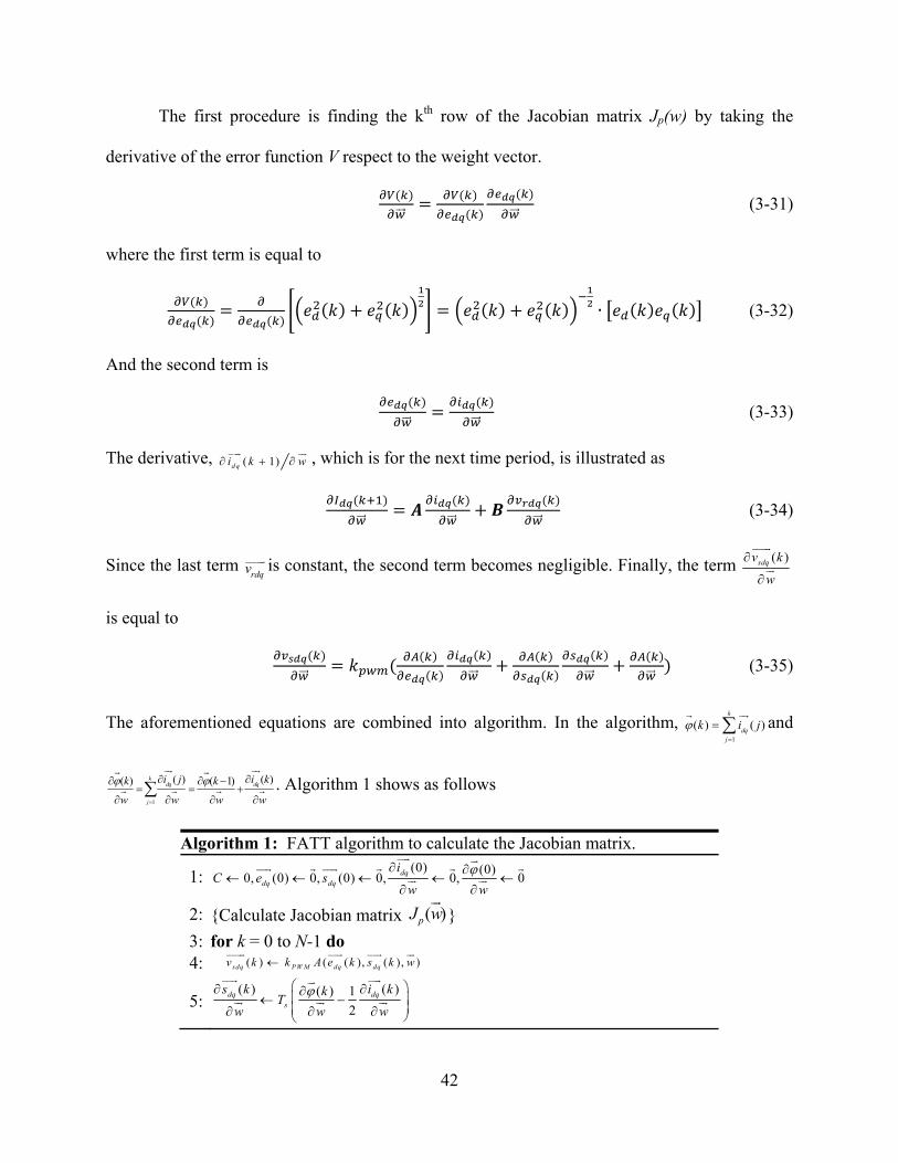
The first procedure is finding the kth row of the Jacobian matrix Jp(w) by taking the

derivative of the error function V respect to the weight vector.

(3-31)

where the first term is equal to

∙ (3-32)

And the second term is

(3-33)

The derivative, ( 1)d qi k w , which is for the next time period, is illustrated as

(3-34)

Since the last term rdqv is constant, the second term becomes negligible. Finally, the term ( )sdqv k

w

is equal to

(3-35)

The aforementioned equations are combined into algorithm. In the algorithm, 1

( ) ( )k

dqj

k i j

and

1

( ) ( )( ) ( 1)kdq dq

j

i j i kk k

w w w w

. Algorithm 1 shows as follows

Algorithm 1: FATT algorithm to calculate the Jacobian matrix.

1: (0) (0)

0, (0) 0, (0) 0, 0, 0dqdq dq

iC e s

w w

2: Calculate Jacobian matrix ( )pJ w

3: for k = 0 to N-1 do 4: ( ) ( ( ), ( ), )sdq PW M dq dqv k k A e k s k w

5: ( ) ( )( ) 1

2dq dq

s

s k i kkT

w w w

43

6: ( ) ( ) ( )( ) ( ) ( )

( ) ( )

sdq dq dqPWM

dq dq

v k i k s kA k A k A kk

w e k w s k w w

7: ( 1) ( ) ( )dq dq sdqi k i k v k

w w w

A B

8: 1 ( )dq dq sdq rdqi k i k v k v A B

9: _( 1) 1 1dq dq dq refe k i k i k

10: ( 1) ( ) ( 1) ( )2s

dq dq dq dq

Ts k s k e k e k

11: ( ( 1))d qC C U e k

12: ( 1)( 1) ( ) dqi kk k

w w w

13: ( 1)( 1) ( 1)

( 1)

dq

dq

i kV k V k

w e k w

14: ( 1)the 1 th row of ( )p

V kk J w

w

15: end for 16: on exit, the Jacobian matrix ( )J w

is finished for the whole trajectory

Table 3.2: FATT algorithm to calculate the Jacobian matrix

3.3.2.4 Training Algorithm

The overall training flow chart is illustrated in Figure 3.8. The parameters in the flow

chart are explained as follows

μmax: maximum available and acceptable μ

βde: decreasing factor (adjust the learning rate during the training)

βin: increasing factor (adjust the learning rate during the training)

Epochmax: maximum number of training epochs

min

/C w

: norm of the minimum acceptable gradient

The final objective of this process is minimizing the DP cost by manipulating μ. The weights are

calculated by using the Cholesky factorization [31], which solves the linear equation twice as

efficient as the LU decomposition. If the following requirements are met, the process will end: a)

44

training epoch = Epochmax, b) μ>μmax, and c) /C w <

min/C w

. As Figure 3.9 illustrates, the DP

cost of the proposed NN controller was stabilized within 100 iterations. The time that took to

train the controller was less than 20 minutes.

( )J w

w

min

C C

w w

max

*w w w

*DP < DP

*DP

in

/ de

*w w

DP

max maxmin

, , , , Epoch ,in de

C

w

w

maxEpoch Epoch

Figure 3.8: Overall flowchart of training NN controller using LM+FATT algorithm

45

Figure 3.9: Average DP cost per trajectory time step for training the NN controller

3.3.3 Simulink Model

The overall schematic is same as shown in Fig. 3.6. The major difference between the

conventional and the proposed NN control is the structure of the current controller. Figure 3.10

shows the block diagram of the NN control while Figure 3.11 shows the mask view of the

current controller. Figure 3.12 illustrates how the aforementioned RNN is translated to Simulink

block.

Figure 3.10: Block diagram of the NN controller

0 100 200 300 400 50010

1

102

103

104

Ave

rage

To

tal C

ost

# of Iteration

46

Figure 3.11: Block diagram of the NN current controller

Figure 3.12: Block diagram representation of RNN control

Hidden Layer Output layer

Input layer

47

CHAPTER 4

MAXIMUM TORQUE PER AMPERE AND FLUX WEAKENING

Generally, there are two operating regions in PMSM drives: constant torque and constant

power region. Figure 4.1 shows a typical torque versus speed graph with two operating regions.

First, when the motor speed is between 0 and its base speed, a PMSM is in constant torque

region. In this region, a PMSM can produce the torque from 0 to its maximum torque. Because

the maximum torque can be sustained constantly in this region, it is called constant torque region.

When the motor speed exceeds its base speed, which occurs when the back-EMF of the motor

reaches the maximum voltage of the system, the maximum allowable torque starts to decrease to

prevent the back-EMF to be exceeded. As the below equation shows, the electrical and

mechanical powers are interrelated to each other.

(4-1)

where T is the motor torque and ω is the motor speed. Since the power is constant as shown in

green curve in Fig. 4.1, this region is called constant power region. In the constant torque region,

many studies utilize a control called maximum torque per ampere (MTPA) control because it

finds the most optimal combination of dq currents to produce the demanded torque [32]. This

technique will not only minimize the copper loss, but also improve the overall driving distance,

since less current is consumed.

In the constant power region, a control called flux weakening control is used. This control

sacrifices the current to increase a motor’s speed range by producing the flux against the flux that

48

is produced by the magnet. Since the induced voltage is proportional to the rate of the flux

respect to time, if the amplitude of the flux is less, the lesser induced voltage will be induced on

the stator. This control is very important because usually, without this control in HEV

application, the maximum vehicle speed is around 50 or 60 mph.

Note that MTPA and FW controls are operating before the proposed NN control. The

main objective is translating the reference torque into optimal d- and q-axis currents for MTPA

control and into adequate d- and q axis currents for FW control.

Figure 4.1: Torque versus speed curve of PMSM with other descriptions

The section is divided into three sections. The first subsection covers the general

overview of two controls while the next two sections epitomize the MTPA control scheme and

the flux weakening control, respectively.

4.1 General operation of PMSM

As Figure 4.2a shows, the motor operation is divided into four sections. As the figure

illustrates, four sections are divided by three different speeds, ω1 to ω3, which are called a base

49

speed, a rated speed, and a second-breakdown speed, respectively. Fig 4.2b illustrates the four

sections in id, iq current contour. This subsection will cover how these sections are divided.

Figure 4.2: a) Torque and speed curve with four different regions b) Segmentation of operation

region for current contour region [32]

50

The first section occurs between 0 and ω1, which is a base speed. The concept of the base

speed begins with voltage-limit ellipse and current-limit circle. Usually, the inverter limits the

current rating while the battery determines the voltage rating. The mathematical representations

of these ratings are

(4-2)

(4-3)

where Is and Us are the amplitudes of operating current and voltage, respectively. If ohmic

voltage drops across the stator winding are neglected in Eq. 2-18, Eq. 4-2 can be rewritten in

terms of the motor parameter

(4-4)

The concept is more clarified if Eq. 4-4 is rewritten in an ellipse equation.

1 (4-5)

where a and b are the length of the semi-major and semi-minor axis, respectively, as shown in

Figure 4.3. Eq. 4-5 clearly shows that if a and b are decreased, the ellipse will shrink. Likewise,

if the speed is increased, Umax/Ldωe and Umax/Lqωe are decreased; then, the ellipse will shrink.

By using Eq. 4-4, the base speed can be calculated. To simplify the calculation, the inductances

and flux linkage constant are assumed to be constant. However, in reality, these values alter as

the motor operates. If the motor parameters are constant, the terms that are changing in Eq. 4-4

are d- and q-axis currents and the speed. If the speed is below the base speed, the value of d- and

q-axis currents can be found by using MTPA method while if the speed is above, different

calculation methods have to be used. These methods will be covered in next subsection. Before

51

that, Figure 4.4 illustrates a typical curve of MTPA control with voltage-limit and current-limit

ellipse in id, iq plane.

Figure 4.3: Ellipse

Figure 4.4: Voltage and current limit circle with constant torque curve and MTPA for IPMSM

[32]

52

If the speed exceeds the base speed, the motor operation is in the second section. This

section operates between the base speed and ω2, which is a rated speed. The rated speed is a

speed where voltage-limit ellipse, current-limit circle, and constant torque curve meet. When the

motor is in this region, MTPA control cannot be used. Instead, the reference torque moves along

the voltage-limit ellipse within the current-limit circle to prevent the back-EMF to exceed the

maximum voltage. Therefore, optimal control cannot be used. Figure 4.2b shows the

aforementioned behavior in id, iq plane.

When the motor speed exceeds the rated speed, the motor now operates in third section.

In third section, as Fig. 4.2b shows, it moves along the current-limit circle. Like in the second

section, optimal control cannot be used.

If the motor speed exceeds a second-breakdown speed, the motor operates in last section.

In this region, the reference torque curve intersects the voltage limit tangentially; thus, different

method needs to be used. As Fig. 4.2b shows, a maximum torque per flux line is used for the

reference torque to be followed.

4.2 MTPA Algorithm

Among many published controls, this thesis chose MTPA control because 1) it uses both

d-and q-axis currents for control 2) minimizes the copper loss, which is one of dominant losses

in the motor [32], and 3) quite simple relative to other methods. In this thesis, three MTPA

controls of IPMSM are covered.

The concept of MTPA control begins with the stator dq voltage equations of PMSMs (Eq.

4-6) and the electromagnetic torque equation (Eq. 4-7). The detailed explanations of these

equations were covered in Chapter 2.

53

0 (4-6)

(4-7)

where vsdq is the stator dq voltage; Rs is the stator resistance; ωe is the electrical angular velocity;

Ldq is the stator dq inductance; λfd is the flux linkage constant; Tem is the electromagnetic torque;

and p is the pole pairs. If the motor is SPMSM, the electrodynamic torque equation is only

dependent on the q-axis current because the stator dq inductances are almost equaled to each

other; thus, the reluctance torque, which is the second portion of Eq. 4-7, is ignored. Thereby, the

electromagnetic torque of SPMSM can be written as

(4-8)

Unlike SPM machine, IPM machine has different d- and q-axis inductances. This means

that the second portion in Eq. 4-7 cannot be ignored; thus, the d-axis current has to be included in

the calculation to control the motor efficiently.

A MTPA control for SPM machine is very easy, since the electromagnetic torque is only

dependent on the q-axis current, as shown in Eq. 4-8. On the other hands, implementing a MTPA

control for IPM machine is hard because the electromagnetic equation is dependent on both d-

and q-axis currents. Thus, many literatures are still researching MTPA controls for IPM machine.

Among published literatures, three MTPA controls are covered as follows.

The first MTPA control is based on look-up table, which is widely used in many

applications because of simplicity. The values of d- and q-axis current are calculated on the basis

of the required torque and speed a priori. However, it will not provide accurate result because,

generally, constant motor parameters are used to calculate the data. If variable motor parameters

are included in the calculation, the dataset will be too large to be implemented.

54

In lieu of look-up table method, the second control is based on real-time calculation.

Most studies use these equations to calculate the d- and q-axis current [40] because of simplicity.

(4-9)

(4-10)

where Is is the reference current that changes. Usually, a PI controller is used to produce the

reference current. However, this control is only suitable when the reference input is speed, but

not suitable for applications that require reference torque as input. Generally, the motor

controller in EV uses the reference torque as its input, which is produced by a controller called

supervisory controller. Thus, this control will not covered in details.

The third method covers above weaknesses by using Ferrari’s method. This method

receives the torque as its reference and converts to corresponding d- and q-axis currents by

solving quartic equations in real time [32]. This also finds the optimal value by finding the

minimum value. In constant torque region, the constrained minimization problem is formulated

as

Minimize

32

The Lagrangian for this problem is formulated as

, , (4-11)

in which λ is a Lagrangian multiplier. Then, the conditions for minimization are defined as

0 2 (4-12)

0 2 (4-13)

55

0 (4-14)

Then, the quartic polynomial equations of the IPM machine is

0 (4-15)

where , , , .

The general solution is given as

∗ (4-16)

∗

∗ (4-17)

1 4 ∗ 4 ∗ (4-18)

1 4 ∗ (4-19)

(4-20)

2 (4-21)

2 (4-22)

2 ∗ ∗

∗ (4-23)

∗ ∗ ∗ ∗ ∗ ∗

∗ (4-24)

1, , ∗ 4 ∗ ,

4 ∗ ∗ ∗ (4-25)

4.3 Flux Weakening Algorithm

When the motor speed exceeds the base speed, the flux weakening control is needed to

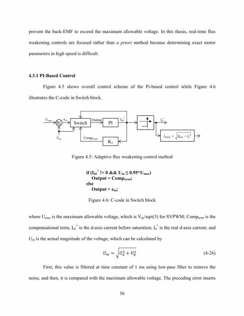
56

prevent the back-EMF to exceed the maximum allowable voltage. In this thesis, real-time flux

weakening controls are focused rather than a priori method because determining exact motor

parameters in high speed is difficult.

4.3.1 PI-Based Control

Figure 4.5 shows overall control scheme of the Pi-based control while Figure 4.6

illustrates the C-code in Switch block.

Figure 4.5: Adaptive flux weakening control method

if (Id1* != 0 && Um ≤ 0.95*Umax)

Output = Compterm; else

Output = em;

Figure 4.6: C-code in Switch block

where Umax is the maximum allowable voltage, which is Vdc/sqrt(3) for SVPWM; Compterm is the

compensational term; Id1* is the d-axis current before saturation; Id

* is the real d-axis current; and

Um is the actual magnitude of the voltage, which can be calculated by

(4-26)

First, this value is filtered at time constant of 1 ms using low-pass filter to remove the

noise, and then, it is compared with the maximum allowable voltage. The preceding error inserts

PI

K1

Switch Umax

Um CompTerm

em Output Id1* Id

*

∗

57

into Switch block. The Switch block determines corresponding output by using the code in Fig.

4.6, and then, this output is inserted to the a PI controller. The output of the PI controller is

saturated between 0 and negative infinity to pass only the negative value. Finally, the maximum

q-axis current is computed to prevent over-current. For PI gains, 20 and 200 were used,

respectively.

4.3.2 Hysteresis Discrete Control

The origin of this control is from a bang-bang controller, also known as a hysteresis

controller, which is a feedback controller that switches between two known states. This

controller is implemented to calculate the d-axis current by using below equation.

∗ ∗ 1 0.1 ∗ 100 (4-27)

where id(k-1) is the past value of id(k). The operation of this controller is simple. If the reference

voltage exceeds the maximum, the second portion decreases the current value with respect to the

error between reference and maximum voltage. However, the downside of this controller is that

like other hysteresis controller, the d-axis current changes in sawtooth waveform as shown in Fig.

4.6.

4.3.3 Ferrari’s Method Control

Ferrari’s method is used to determine the d-axis current in flux weakening region.

Theoretically, this control ensures to get optimal d- and q-axis currents for different constraints.

However, the downside of this method and other optimal method is that it requires accurate

parameter values to determine reference d- and q-axis current. Another downside of this control

is that it produces complex numbers. The complex number was found when square root of Q3

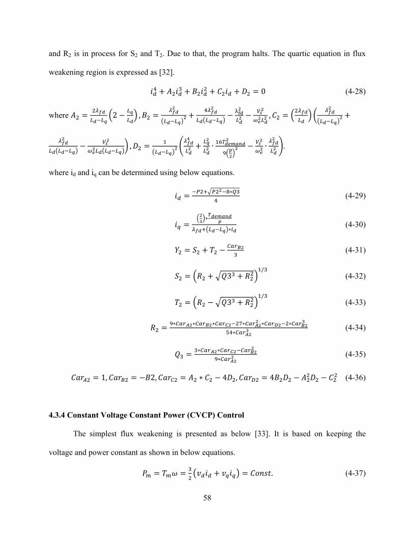
58

and R2 is in process for S2 and T2. Due to that, the program halts. The quartic equation in flux

weakening region is expressed as [32].

0 (4-28)

where 2 , ,

, ∙ ∙ .

where id and iq can be determined using below equations.

∗ (4-29)

∗

∗ (4-30)

(4-31)

3/

(4-32)

3/

(4-33)

∗ ∗ ∗ ∗ ∗ ∗

∗ (4-34)

∗ ∗

∗ (4-35)

1, 2, ∗ 4 , 4 (4-36)

4.3.4 Constant Voltage Constant Power (CVCP) Control

The simplest flux weakening is presented as below [33]. It is based on keeping the

voltage and power constant as shown in below equations.

. (4-37)

59

Const. (4-38)

λ . (4-39)

. (4-40)

where vqb, iqb, and ωbase are base voltage, base current, and base speed, respectively. For SPM

motor case, the base current is the maximum current while for IPM motor application, the base

current differs. If Eq. 4-37 and 4-40 are combined, the d and q-axis current can be expressed as

1 (4-41)

(4-42)

More details of this control and other controls can be found in [33].

60

CHAPTER 5

ELECTRIC VEHICLE MODEL

The dynamic model of an EV system is implemented in MATLAB Simulink/

SimPowerSystems and SimDriveline environment. Further, the corresponding EV model is

constructed out of current commercial components, first, to simulate more realistically and

second, to observe the effectiveness of the neural network controller with the off-the-shelf

electric motor. Table 5.1 shows the description of the components, whereas Table 5.2 denotes the

overall specification of EV. Moreover, the inverter block from Opal-RT is implemented, instead

of from SimPowerSystems, because the inverter block from Opal-RT simulates faster than using

the inverter block from SimPowerSystems.

The section is divided into four subsections. Each subsection introduces the four

individual blocks, the functions of the block, corresponding off-the-shelf component(s) if

applicable, and SimPowerSystem or SimDriveline components. Before diving into the

discussion, the overall schematic of the EV is shown in Fig. 5.1 while Fig. 5.2 illustrates the

overall block diagram of the EV. Lastly, the simulated models in Simulink are shown in Fig. 5.3.

61

Figure 5.1: Overall schematic of the EV

Figure 5.2: Overall block diagram of the EV

Figure 5.3: Overall block diagram of the EV in Simulink

DriveCycle Driver Machine/Inverter

Shaft/ Differential

Front Tire

Chassis

Rear Tire

Brake

Battery

Ref. Spd (m/s) APP

(%)

Torque (Nm)

Vdc (V)

Left/Right Torque (Nm)

Normal/ Longitudinal

Force (N)

Normal/ Longitudinal Force (N)

Brake

Brake Force (N)

Vehicle Spd (m/s)Motor Spd

(rad/s)

Brake Force (N)

Vehicle Spd (m/s)

62

Component Simulink Block Name Part Name

Motor Permanent Magnet Synchronous Machine

(SimPowerSystem) Parker GVM210-150P

[34] Inverter IGBT/Diode in Universal Bridge (SimPowerSystem) Rinehart PM100DX [35]

ESS Battery/Resistor/Ideal Switch (SimPowerSystem) A123 7x15s3p pack [36]Differential Differential (SimDriveline)

Chassis Vehicle Body (SimDriveline) Midsize sedan Tire Tire (Magic Formula) (SimDriveline) 215/55R17 [37] Shaft Flexible Shaft (SimDriveline) Brake Double Shoe Brake (SimDriveline) Hydraulic

Table 5.1: Part and Simulink block name for components

Parameter Description ValuesVehicle Dynamic

Mveh Total mass of the vehicle 1,560 kgCrr Coefficient of rolling resistance 0.01Cdrag Coefficient of aerodynamic drag 0.35CdA Frontal area 0.76 m2

ρ Air density 1.2 kg/m3

Tire Rwheel Wheel radius 0.324 mα, β, A, B, C See the description in Section 5.

Motor Ppeak and Pcont Peak/ Continuous output power 100/70 kWTpeak and Tcont Peak/ Continuous output torque 256/122 Nmωmax and ωrated Max/ Rated motor speed 7,500/5480 RPMRs Stator resistance 18.5 mΩLd and Lq d and q-axis inductance 0.22 and 0.32 mHλf Flux linkage constant 0.0595 WbP # of poles 12Jeq Rotor inertia 0.028 kg·m2

Battery (7x 15s x 3p) Vnom Nominal voltage 340 VIndis and Inchg Nominal discharge and charge current 180/60 AIpdis and Ipchg Peak discharge and charge current 612/300 ACap Pack capacity 58.8 AhEnom Pack energy capacity 18.9 kWh

Shaft and Differential FDR Final drive ratio 8.2Smat Shaft material Al alloySdia Shaft diameter 65mmSlength Shaft length 761mm

Table 5.2: EV specification

63

5.1 Driver

The simulation starts its operation from Driver block. A block diagram of the driver

system is given in Figure 5.4. The primary purpose of this block is producing the applied pedal

position (APP), which describes how much the pedal is pushed by the driver. The range of the

APP is -100% to 100%. The negative APP denotes braking. When the APP is negative, either

hydraulic or regenerative, or both, braking are initiated, depending on the condition.

Inputs to the driver system are reference and actual speed of the vehicle while outputs are

APP in percent and reference hydraulic brake force. For this simulation, three different

drivecycles are used for the reference speed: UDDS, HWFET, and US06. Fig. 5.5 shows UDDS,

HWFET, and US06, respectively. An UDDS drivecycle provides common urban drive trace

while a HWFET denotes to highway driving. Lastly, an US06 is for aggressive city driving plus

highway. The actual vehicle speed is calculated from chassis and tire block.

Figure 5.4: Block diagram in Driver block

64

a) UDDS

b) HWFET

c) US06

Figure 5.5: a) UDDS, b) HWFET, and c) US06 drivecycle

0.0

10.0

20.0

30.0

40.0

50.0

60.0

0 500 1000 1500

Speed (mph)

Time (s)

0

10

20

30

40

50

60

70

0 200 400 600

Speed (mph)

Time (s)

0

10

20

30

40

50

60

70

80

90

0 100 200 300 400 500 600

Speed (mph)

Time (s)

65

First, the driver block receives two speed inputs and converts their units from mph to m/s.

Then, these converted inputs are subtracted and applied to a PI controller. The proportional (P)

and integral (I) gains that were used are 50 and 1, respectively. The output of the PI controller is

APP. Then, this APP is applied to Stateflow block, which is a control logic tool used to emulate

the state machine within Simulink model. The main role of this block is determining the required

hydraulic brake force from APP. The mask view of the Stateflow diagram is shown in Fig 5.6.

Detailed information is covered in subsection 5.4.2.

Figure 5.6: Stateflow diagram of the braking shift logic

5.2 Motor Drive and ESS

The main objective of this block is translating the APP into the actual motor traction

torque. Fig. 5.7 illustrates the overall block diagram of the motor drive and energy storage

system (ESS) block while Fig. 5.8 shows the overall schematic of the motor drive. As Fig. 5.7

shows, four blocks are identified: max torque, APP2RefTrq, Controller, Motor and Inverter, and

ESS.

66

Figure 5.7: Block diagram in Motor Drive block

Figure 5.8: Overall schematic of motor drive

5.2.1 ‘Max torque’ Block

A block diagram of max torque block is shown in Fig. 5.9. The main purpose of this

block is determining the maximum allowable torque. As Fig 5.9 illustrates, two look-up tables

are connected with the input vehicle speed, where an upper look-up table contains the continuous

torque values while a lower table contains the peak torque values. The temperature is taken into

account by constraining the time allowed above continuous torque. A block called “Heat index”

is used to accomplish the tasks. The mask view of this block is given in Fig. 5.10. The following

equation is utilized to find the shifting point.

MTPA

APP (%)

Motor Spd (rad/s)

T* (Nm)

Max Torque (Nm)

Vdc (V)

Id*

Iq*

αβ dq

SVPWM

vd*

vq*

vα*

vβ*

IPM

sq

sd

ed

eq

abc dq

Iabc

Id

Iq

θ

θ

67

. 1 (5-1)

where Torqueactive is the actual motor torque; Torquecont is the continuous motor torque; and tmax

is the maximum allowable time for maximum torque to be on. In this model, 10 second is used

for tmax. The range of the heat index is between 0 and 1. If the heat index is 0, the peak torque is

utilized while if it is 1, the continuous torque is used. If the heat index is between two values, the

torque linearly decreases from the peak torque to the continuous torque. Simply saying, even if

the driver still wants to maintain the full throttle of the motor after tmax, this calculation prevents

the driver to doing so in order to protect the motor. Furthermore, this block also works properly

when the motor operates as a generator.

Figure 5.9: ‘Max torque’ block diagram

68

Figure 5.10: ‘Heat index’ block diagram

5.2.2 ‘APP to Reference Torque’ Block

A block diagram of APP2RefTrq block is displayed in Figure 5.11. The role of this block

is receiving the maximum torque from max torque block and APP in percent, and converting to

the reference torque by multiplying two signals as in Fig. 5.11. Since APP is in percent, it is

multiplied by 0.01 to change decimal value.

Figure 5.11: ‘APP2RefTrq’ block diagram

5.2.3 ‘Controller’ Block

A block diagram of the controller block is shown in Fig. 5.12. The objective of this block

69

is translating the reference torque into corresponding PWM signal for the inverter. Inputs to the

system are the motor speed, three-phase currents, reference torque, and dc-link voltage. Output is

PWM signal.

Figure 5.12: ‘Controller’ block diagram

After receiving above inputs, the block translates the demanded torque to reference d and

q-axis currents by using MTPA control that was discussed in Chapter 4. Simultaneously, the

block transforms three-phase currents to d and q-axis and calculates the angular position of the

motor through integrating the motor speed. Note that Ferrari’s method is used for MTPA control

in this thesis. Then, those signals are applied to the proposed NN controller. The detailed

descriptions of the proposed NN controller are explained in Chapter 3. Note that the error is

equaled to actual minus reference, not the other way around. Then, the NN controller produces

the normalized d- and q-axis voltage. After de-normalizing the voltage by multiplying the space

vector PWM (SVPWM) gains, the d- and q-axis voltages are converted to three-phase abc

voltages. Lastly, through SVPWM, 6 pulses of PWM signals are calculated.

5.2.4 ‘Motor and Inverter’ Block

70

A block diagram of motor and inverter block is given in Fig. 5.13. Inputs to the system

are the shaft speed, 6 SVPWM pulses, and DC-link voltage of ESS. Outputs are three-phase

current and motor torque. As Fig. 5.13 illustrates, the inverter from Opal-RT and the motor from

SimPowerSystem library are used. Further, notice that the motor takes the speed as its load input,

rather than the torque. The primary reason is that the torque is the factor is changing. If the speed

was changing, the motor will take the load torque.

The operation of this block is simple. First, the block receives the pulses from the motor

and controller block and applies to the inverter for controller. The DC side of the inverter is

connected with ESS. With using above inputs, the inverter transforms DC input to AC output

accordingly. Then, these AC signals flow through the measurement tool and finally apply to the

motor. Lastly, the motor produces the electromagnetic torque.

Figure 5.13: Inside view of the ‘motor and inverter’ block

As for the electric motor component, Parker GVM210-150P was chosen. The motor

specification is given in Table 5.2. The primary reason to choose this motor was it possesses 1)

reasonable overall peak, 2) continuous power density, 3) operating voltage rating, and 4) low

torque ripple for EV application. Fig. 5.14a shows the actual motor while Fig. 5.14b the graph

that consists of base speed, peak power, and rated power [34].

71

For the inverter component, Rinehart PM100DX inverter was used because it not only

meets the requirement of the EV system, but also has reasonable size to be fitted in actual EV

platform. Fig. 5.15 shows the drawing of PM100DX inverter [35]. As Fig. 5.15 shows, the size

of the inverter is only 314 x 200 x 87 mm3.

a)

b)

Figure 5.14: a) Actual motor and b) specification in graph [34]

72

Figure 5.15: Drawing of PM100DX inverter [35]

5.2.5 ‘ESS’ Block

The last block to discuss is an energy storage system (ESS). Generally, five electrical

components are formulated to structure the ESS. They are a current sensing modules (CSM), a

battery control module (BCM), an electronic distribution module (EDM), and an emergency

disconnect switch (EDS). Table 5.3 describes the functionality of each component.

Name Description CSM Measures the current through magnetic field. If the current and elapsed time exceed

limit value, it sends an alert to BCM. Then, BCM orders EDS to open its switch. BCM Functions as a brain. It disconnects the ESS from the system when the current and

voltage exceeds its limit. It communicates with supervisory controller through CAN. EDM Consists of three contactors and one resistor. Three contactors are positive, negative,

and pre-charge contactors. Pre-charge function limits inrush current. EDS Disconnects the current flow when BCM alerts. It is usually located between

modules. See Figure 5.16.

Table 5.3: Descriptions of ESS components

73

A block diagram of ESS is displayed in Fig. 5.16. The primary purpose of this block is

providing the electrical energy to corresponding motor drives. In lieu of implementing five ESS

components, this thesis utilizes four components to emulate the performance of ESS for

simplicity. They are batteries, EDM, EDS, and CSM. First, the battery block from

SimPowerSystems library is used for battery. The required parameters of the battery are

extracted from the datasheet. Second, one 25 Ω resistor and three ideal switches in

SimPowerSystems library are used to model the EDM, where the resistor is representing the pre-

resistor while two upper and one lower ideal switches represent the pre-contactor and main

positive contactor and negative contactor, respectively. Third, one ideal switch is used to model

the EDS. If state of charge (SOC) is less than 20%, the switch will open to prevent the battery to

be full discharged. Lastly, the current measurement block in SimPowerSystem library is used to

model the CSM.

Figure 5.16: Overall block diagram of the ESS

As for the ESS component, A123 ESS was used. The battery is formulated into 7x15s3p

structure, where 7 denotes the number of module, 15s refers to 15 cells in series, and 3p conveys

parallel of three. The multiple concatenated cells make a module while the multiple connected

74

modules construct a pack. Usually, the voltage rating of a cell is on the order of one to six volts.

Fig. 5.17a shows the structure of 1 module while Fig. 5.17b shows an actual A123 ESS, which

includes 7 modules and other supplementary components.

Figure 5.17: a) Schematic of 1 module and b) overall ESS [35]

5.3 Shaft and Differential

The next block to be discussed is ‘shaft and differential’ block. The primary purpose of

the shaft is connecting the motor and differential while the objective of the differential is

splitting the shaft torque into two torques for front wheels. Note that only longitudinal motion

was considered. Thus, the differential in this thesis will halve the input torque evenly. However,

in real environment, the torque is unevenly split when the vehicle is on the curve. Fig. 5.18

shows the overall block diagram of ‘Shaft and Differential’ block.

As Fig. 5.18 shows, two inputs are used. The first input is the motor torque while other is

the actual vehicle speed in meters per second. First, to accommodate proper connectivity

between Simulink and SimDriveline, Simulink to PS torque block is used. Like the name

a) b)

75

implies, the main purpose of this block is translating Simulink signal to mechanical signal. Fig.

5.19 illustrates the Simulink to PS Torque block diagram.

Figure 5.18: Overall block diagram of ‘Shaft and Differential’ block

Figure 5.19: Simulink to PS Torque block diagram

Then, this mechanical torque is now applied to the motor shaft. A block called Flexible

shaft in SimDriveline is used to model the actual shaft. As it shows, the total length of the shaft

is 1,386 mm. Two shafts were used to prevent the shaft to be shattered from the rotational force,

and U-joint is connecting two shafts. The diameter of first shaft that is connected with the motor

is 60 mm while the second that is connected with the differential is 65 mm. Other parameters of

the shaft can be found in Table 5.2. Then, the output torque of the shaft splits into two torques by

76

using differential, which is also provided by SimDriveline library. The value 8.2 was used for

final drive ratio (FDR).

The second task of this block is translating the actual vehicle speed from the chassis to

the motor speed. This is easily achieved by utilizing this equation.

(5-2)

where Rtire is the radius of the tire.

5.4 Tire, Chassis, and Brake

This subsection contains four tires, four hydraulic brakes, and a vehicle body. The origin

of these components is from SimDriveline. The primary purpose of this block is modeling the

function of tires, hydraulic brakes, and chassis. Table 5.1 denotes the name of SimDriveline

components with associated components in real life while Fig. 5.21 shows the inside view of

‘Tire, chassis, and brake’ block.

As Fig. 5.21 illustrates, inputs to the system are hydraulic brake command from the

driver block and two torques from the ‘shaft and differential’ block. Output is the actual vehicle

speed in meters per seconds. First, the mechanical signals from the differential and hydraulic

brake command are applied to the front left and right wheels. Then, the wheel block produces

corresponding signals to vehicle body. These signals are explained in following sections.

77

Figure 5.20: Overall diagram of ‘Tire, Chassis, and Brake’ block

5.4.1 Tire

A block diagram of wheel block is given in Fig. 5.22. As for the tire, the wheel block in

SimDriveline library is used. This block is based on the magic formula, which is invented by

Hans BastiaanPacejka and called “magic” because only 10 to 20 coefficients are used to

represent the vertical load force on the tire, camber angle, and slip angle [38]. The following

equation is the general form of the magic formula:

( ) sin arctan[ (1 ) arctan( )]R k d c b e k e bk (5-3)

in which b, c, d, and e are fitting constants while R(k) is a resultant force from a slip parameter k

[38].

First, the model takes the input torque from the differential in port A and transmits the

thrust generated by the tire to the remainder of the vehicle body through port H. Then, the

vehicle body calculates the normal force acting on the tire and feeds to port N [39]. Further,

pressure and velocity dependent rolling resistance is included for more realistic The explanation

78

can be found in [39] while the associated coefficients are -0.4736, 1.031, 6.839e-2, 1.65e-4, and

4.125e-7 for α, β, A, B, and C, respectively. Finally, since no traction force is transmitted to the

rear tire, at port A, a simple inertia block is inserted to represent free rolling.

Figure 5.21: Inside view of ‘wheel’ block

5.4.2 Brake

One of the distinguished factors of the EV is the regenerative braking, which accumulates

the electricity by providing the negative torque to the motor when the vehicle is decelerating.

However, having only regenerative braking is not sufficient to meet the total demanded braking

force, especially when sudden braking is needed. Further, not only that, the regenerative braking

79

technique cannot be used when the battery is near to the full charge and is not efficient to use

when the vehicle speed is below 10 mph. As a result, the conventional hydraulic brake is still

required to compensate the aforementioned problems.

When both braking system is used, there are two possible brake combinations: series and

parallel braking. The advantage of the series braking is that the optimal braking combination can

be achieved while the advantage of the parallel braking is simple construction. However, the

study showed that the parallel braking cannot recover the maximum energy [40].

In this paper, simple series braking is considered, and these are the rules. Only

regenerative braking is applied when APP is below -50% while vehicle speed is above 10 mph,

and when the vehicle speed is below 10 mph, only hydraulic braking is applied. If the vehicle

speed is above 10 mph while APP is above -50%, the motor regenerates only -50% of the total

braking force while others are compensated from the hydraulic braking.

A block called Double-Shoe Brake in SimDriveline library is used to emulate the

mechanical brake. As Fig. 5.22 shows, it has two connections: Port S and F, where Port S is

connected with the input of the tire, which is the output of the differential, and Port F is

connected with the demanded hydraulic force from the Driver block. This block takes the

demanded brake force and then, translates the physical signal into mechanical signal, so it can be

applied in the overall system. This model was chosen because one of the EV examples in

Simulink used this as its brake.

5.4.3 Chassis

A block called Vehicle body in SimDriveline library is used to model the chassis. The

primary objective of this block is to calculate the vehicle longitudinal velocity. This is achieved

80

by using the total traction force equation.

21( ) sgn( ) sin( )

2grade

aero

x w x w rr xdrag dA veh veh

FF

F C C V V V V F M g M V (5-4)

where F is the total traction force, Faero is the aerodynamic drag force, Vx and Vw is the velocity

of the vehicle and wind, respectively, Frr is the rolling resistance, Fgrade is the grade resistance

force, φ is the angle of the grade, and Vx’ is the acceleration. The vehicle is assumed to be

midsize car; thus, the vehicle mass is 1,560 kg, which is average of midsize car [41]. And frontal

area and drag coefficient is changed as shown in Table 5.2. Other than these three parameters,

default values are used for other parameters. Through this equation, the vehicle speed is

calculated.

The next calculation is determining the normal force for the front and rear-axle wheel and

can be found by using below equations.

( sin( ) ) cos( )( )

aero xveh veh vehzf

h F W M V b WF

n a b

(5-5)

( sin( ) ) cos( )( )

aero xveh veh vehzr

h F W M V a WF

n a b

(5-6)

in which h is the height of vehicle, which is center gravity above the ground, a and b is distance

of front and rear axles from the normal projection point of vehicle CG, and Wveh is the weight of

the vehicle, which is mass of the vehicle times the gravity. These normal forces are applied to the

wheels.

81

CHAPTER 6

SIMULATION RESULTS

For overall simulation, MATLAB Simulink is used because it has 1) easy graphical user

interface (GUI), 2) simple data handling and storage, 3) extensive component libraries, such as

mechanical, electrical, vehicle, and others, and 4) the flexibility in transition between physical

and other signals. Three different simulations were conducted to observe the effectiveness of the

proposed ANN controller. In the first, a basic feedback speed-loop control for SPMSM was

observed when the motor 1) is accelerating and decelerating, 2) experiences parameter variation

3) experiences load torque variation, and 4) is in high speed. In the second, a basic feedback

speed-loop control for IPMSM was tested to observe the performance in same conditions as in

the first simulation. In addition, for both simulations, the conventional PI control was also

observed to compare with the proposed control. In the last simulation, the NN control for

IPMSM was implemented in electric vehicle model as illustrated in Chapter 5.

6.1 SPMSM Simulation Result

6.1.1 Motor Parameter and Simulation Setup

First, 0.2 kW SPMSM motor was used to validate the controls. The specifications of 0.2

kW motor are given in Table 6.1.

Conventionally, most motor drives have widely employed analog-based controller.

However, with the advent of the digital signal processor (DSP) and microcontroller (μC), nearly

82

all of motor drives employs digital controller to control the motor because the digital controller

offers 1) more powerful performance and 2) flexibility than the analog-based controller. Further,

generally, the digital controller samples the analog signal at certain controller. Further, generally,

the analog signal at certain rate. Throughout this thesis, 0.1 ms sampling rate was used because it

is not only reflecting typical sampling rate for motor drive, but also not causing any “data freeze”,

especially in hardware experiment.

Parameter Value Units Rated Power 200 W

dc voltage 42 V Permanent magnet flux 0.0154 Wb Inductance in q-axis, Lq 0.255 mH Inductance in d-axis, Ld 0.255 mH

Stator copper resistance, Rs 0.22 Ω Inertia 0.07 kgm2

Damping coefficient 0.01 Pole pairs 4

Table 6.1: 0.2 kW PMSM parameter in simulation and hardware study

Unlike the digital controller, the inverter and motor do not have any sampling rate; thus,

these components need another solution. For the solution, 2 μs sampling rate was used to model

the continuous state as close as possible. Lower sampling rate is better, but it increases the

simulation time, simultaneously.

As shown in Fig. 3.1 and 3.10, both controllers are using PI controller for their speed-

loop controller. To tune PI gains, first, a cross-over frequency of the speed loop was chosen.

Upon speculations, it was concluded that 2.5 kHz provided the most adequate response. Then,

phase margin was chosen. Upon speculations, 60 degree was chosen for same reason. Then, the

following equations were used to determine the initial PI gains of the speed loop controller.

2500 (6-1)

83

∗ (6-2)

60 ∗ (6-3)

(6-4)

∗ (6-5)

∗ (6-6)

where Jeq is the inertia of the motor. With having these initial PI gains as base values, slight

modification was done. As a result, the final Kp and Ki were 3.83 and 79.12, respectively.

Likewise, the PI gains of the current controller for the conventional controller were

calculated. Because the inner current loop controller has to respond faster than the outer speed

loop controller, the crossover frequency of the current controller had to be a magnitude larger

than the crossover frequency of the speed controller. For phase margin, same value as in speed-

loop controller was used. The following calculations were used to determine initial PI gains.

ω 25000 (6-7)

60 ∗ (6-8)

∗ (6-9)

∗‐ ∗

(6-10)

∗ (6-11)

Similarly, the calculated PI gains were modified. As a result, for the PI gains, 1.38 and 199.8

were used, respectively.

84

Aforementioned, total of four tests were conducted to observe the performance of the

proposed controller and conventional controller. They are acceleration and deceleration test, load

torque variation test, parameter variation test, and flux weakening test. Note that the initial load

torque of 0.1 Nm was used.

First, the acceleration and deceleration test was conducted as follows. At t=0.56 s, the

input speed was increased from 0 rad/sec to 100 rad/sec, and then stayed at 100 rad/sec for 1

second. At t=1.56s, the speed was decreased to 50 rad/sec and retained its value for 1 second. At

t=2.56 s, the speed was increased to 200 rad/sec and decreased again to 100 rad/sec at t=3.56 s.

After the acceleration and deceleration test, the load torque was varied as follows. At

t=4.36 s, the load torque was changed from 0.1 to 0.3 Nm. At t=5 s, the load torque was dropped

to 0.1 Nm.

After the load torque variation test, the parameter variation test was conducted as follows.

At t= 5.5 s, the stator resistance, synchronous inductance, and flux linkage constant was changed:

the stator resistance was doubled while the inductance and flux linkage constant was reduced

20%.

Lastly, the flux weakening control was tested for both controllers. At t=6.75 s, the

reference speed was accelerated at a rate of 150 rad/s2 until it reached just slightly below the

maximum speed, which is about 400 rad/s. At t=9.75 s, the reference speed was decreased to 200

rad/s to check whether the control can return to normal control from the flux weakening control.

6.1.2 Results

The traction result of speed, dq currents, abc currents, and normalized system voltage for

both conventional and neural network controller are shown in following figures (from Figure 6.1

85

to 6.7), respectively.

As the figures show, both controllers perform similarly until the flux weakening test. As

Fig. 6.1 shows, when the reference speed is about 250 rad/s, the conventional control loses the

stability. Even though the PI gains for conventional control were changed in numerous times,

none of the PI gains could solve the problem. However, unlike the conventional control, ANN

control exhibits very stable speed traction in high speed region. When the motor reaches 400

rad/sec, as Fig. 6.2 shows, the d-axis current is producing the negative value to prevent the back-

EMF to exceed the maximum voltage (Fig 6.6).

Figure 6.1: Speed traction of SPMSM (simulation)

0 2 4 6 8 10 12-100

0

100

200

300

400

500

600

Time (s)

Spe

ed (

rad/

s)

Reference

ANNConventional

2.7 2.8 2.9

180

200

220

5 5.5 6

100

102

104

86

Figure 6.2: ANN d- and q-axis current traction of SPMSM (simulation)

Figure 6.3: Conventional d- and q-axis current traction of SPMSM (simulation)

0 2 4 6 8 10 12-30

-25

-20

-15

-10

-5

0

5

10

15

20

Time (s)

Cur

rent

(A

)

Iq*

IdIq

0 2 4 6 8 10 12-500

-400

-300

-200

-100

0

100

Time (s)

Cur

rent

(A

)

Id*

Iq*Id

Iq

1 2 3 4

-10

0

10

20

87

Figure 6.4: ANN abc current traction of SPMSM (simulation)

Figure 6.5: Conventional abc current traction of SPMSM (simulation)

0 2 4 6 8 10 12-25

-20

-15

-10

-5

0

5

10

15

20

25

Time (s)

Cur

rent

(A

)

Ia

IbIc

0 2 4 6 8 10 12-150

-100

-50

0

50

100

150

Time (s)

Cur

rent

(A

)

Ia

IbIc

88

Figure 6.6: ANN normalized amplitude of voltage of SPMSM (simulation)

Figure 6.7: Conventional normalized amplitude of voltage of SPMSM (simulation)

0 2 4 6 8 10 120

0.2

0.4

0.6

0.8

1

1.2

1.4

Time (s)

V n

orm

aliz

ed

0 2 4 6 8 10 120

0.5

1

1.5

2

2.5x 10

4

Time (s)

V n

orm

aliz

ed

89

6.2 IPMSM Simulation Result

6.2.1 Motor Parameter and Setup

100 kW Parker GVM210-150P IPMSM was used to demonstrate the simulation. Table

5.1 shows the specification of the preceding motor. The PI gains for the speed controller for both

controllers were calculated using the method that was shown above. Likewise, the PI gains of the

current controller were determined.

Same four tests were conducted as follows. First, the acceleration and deceleration test

were conducted as follows. At t=0.5 s, the input speed was increased from 0 rad/sec to 100

rad/sec, and then kept at 100 rad/sec for 0.75 second. At t=1.25s, the speed was decreased to 50

rad/sec. At t=2 s, the speed was increased to 200 rad/sec and decreased again to 100 rad/sec at

t=3 s. Then, the load torque variation was observed.

Then, the load torque variation test was observed. At t=3.5 s, the load torque was

changed from 20 Nm to 100 Nm. At t=4.25 s, the load torque was further increased to 200 Nm

and then, dropped to 50 Nm at t=5 s.

After the load torque variation test, the parameter variation test was conducted. At t= 5.5

s, the stator resistance was doubled while the d- and q-axis inductance was decreased 20% and

30%, respectively. Lastly, the flux linkage constant was reduced by 20%. At 6.5s, the parameter

was changed back to the original values.

Lastly, at t= 7 s, the flux weakening control was tested by increasing the reference speed

at a rate of 200 rad/sec2 until 650 rad/s is reached. Then, the speed was decreased to 300 rad/s at

t= 10.5 s.

90

6.2.2 Results

Fig 6.8 and 6.9 shows the speed traction and dq current traction of both controllers while

Fig. 6.10 and 6.11 illustrates the abc current traction of ANN control and conventional control

for IPMSM respectively. Lastly, Fig. 6.12 shows the normalized system voltage of both

controllers.

For the first and second tests, both controllers showed similar performance as the figures

illustrate. However, for parameter variation test, the conventional controller shows better

response than the proposed controller. As shown in Fig 6.9, the d- and q-axis currents of the

ANN controller are oscillating, but not for the conventional controller. Further, in the flux

weakening control test, Fig. 6.9 shows that the ANN controller uses less d-axis current than the

conventional controller while for q-axis current, the ANN controller uses slightly more current

than the conventional controller. Aforementioned, the d-axis current produces the flux against

the magnet flux to prevent the back-EMF exceeding certain threshold. Larger the d-axis current,

the more the opposing flux is. However, the downside is that if this opposing flux is too large, it

can demagnetize the magnet, where the demagnetization of the magnet causes the motor to be

not operable. Thus, having less d-axis current is better. In Fig 6.9, the ANN controller produces

less d-axis current than the conventional controller; thereby, it can be concluded that the former

controller performs better in high speed than the latter controller.

91

Figure 6.8: Speed traction of IPMSM (simulation)

Figure 6.9: D-and q-axis current traction of IPMSM (simulation)

0 2 4 6 8 10 120

100

200

300

400

500

600

Time (s)

Spe

ed (

rad/

s)

Reference ANN PI

0 2 4 6 8 10 12-300

-200

-100

0

100

200

300

400

500

Time (s)

Cur

rent

(A

)

Id*Iq*

ANN Id

ANN Iq

Conv IdConv Iq

2.15 2.2 2.25 2.3 2.35

199

200

201

4.5 5 5.595

100

105

92

Figure 6.10: ANN abc current traction of IPMSM (simulation)

Figure 6.11: Conventional abc current traction of IPMSM (simulation)

0 2 4 6 8 10 12-400

-300

-200

-100

0

100

200

300

400

Time (s)

Cur

rent

(A

)

Ia

IbIc

0 2 4 6 8 10 12-400

-300

-200

-100

0

100

200

300

400

Time (s)

Cur

rent

(A

)

Ia

IbIc

93

Figure 6.12: Normalized amplitude of voltage of IPMSM (simulation)

6.3 Electric Vehicle

To observe the transient response of the proposed NN controller and performance of the

regenerative and hydraulic braking in EV application, US06-City drivecycle is used because this

drivecycle not only consists of frequent start and stop situation, but also requires the vehicle to

go up to 71 mph. In other words, it was chosen because it represents a very practical and typical

driving condition in the United States. Further, the proposed controller was compared with PI-

based controller, which is widely used in industry, to demonstrate the effectiveness of the

controller.

Fig. 6.13 shows the reference and actual vehicle speed while Fig. 6.14 illustrates the

reference and actual motor torque. The APP and hydraulic brake force, a dotted line, can be

observed in Fig. 6.15. Fig. 6.16 shows the behavior of the d- and q-axis currents. Lastly, Fig.

0 2 4 6 8 10 120

0.2

0.4

0.6

0.8

1

1.2

1.4

Time (s)

V n

orm

aliz

ed

ANN

PI

94

6.17 exhibits the SOC of the battery and APP graph together to show the functionality of the

regenerative breaking.

As Figs. 6.13, 6.14, and 6.15 show, the EV using the proposed NN controller tracks the

reference signal closely and shows similar performance with the EV using PI controller. Further,

Fig. 6.16 validates that hydraulic brake assists the regenerative braking when the above condition

is not met. In addition, when the braking occurs, meaning APP is negative value, the battery is

charged (Fig. 6.17).

Figure 6.13: Speed traction of EV

0 50 100 150 200 250

0

10

20

30

40

50

60

70

80

Time (s)

Spe

ed (

mph

)

Reference

ANN

PI

95

Figure 6.14: Torque traction of EV

Figure 6.15: D- and q-axis current traction of EV

0 50 100 150 200 250-150

-100

-50

0

50

100

150

200

250

Time (s)

Tor

que

(Nm

)

Reference ANN PI

0 50 100 150 200 250-300

-200

-100

0

100

200

300

400

Time (s)

Cu

rre

nt (

A)

Id* Iq* Id (Conv) Iq (Conv) Id (NN) Iq (NN)

96

Figure 6.16: ANN APP and hydraulic braking traction of EV

Figure 6.17: ANN APP and SOC traction of EV

0 50 100 150 200 250-100

-50

0

50

100

Time (s)

AP

P (

%)

0 50 100 150 200 250-300

-200

-100

0

100

Hyd

raul

ic B

rake

For

ce (

kN)

APP Hyd. Brake

0 50 100 150 200 250-100

-50

0

50

100

Time (s)

AP

P (

%)

0 50 100 150 200 25058

58.5

59

59.5

60

SO

C (

%)

97

CHAPTER 7

HARDWARE RESULTS

7.1 Hardware Experiment Component Description

Five components were used to conduct hardware experiment. They are 1) dSPACE

CP/DS1103, 2) Lab-volt inverter, 3) Lab-volt power supply, 4) OP8660 data acquisition

interface, 5) motor dyno kit. Figure 7.1 shows the schematic of the overall hardware experiment

while Figure 7.2 shows the physical hardware setup of the system.

Figure 7.1: Schematic of the hardware experiment

~

Lab-volt 8821

AC Source

Lab-volt

Rectifier Inverter

Data Acquisition

OP8660

PMSM

BLDC7105 ia

ib

ic

DC Gen

DCGEN7105

Vdc

ControlDesk

MATLAB Simulink

dSPACE

CP 1103 I/O Board

Encoder PWM

98

Figure 7.2: Physical wiring of hardware experiment

99

Figure 7.3: dSPACE CP1103 pinout description

For a digital signal processor (DSP) controller, dSPACE CP/DS1103 board was used. As

Fig. 7.3 shows, the board contains multiple on-board peripherals such as analog-to-digital (ADC)

converters, digital-to-analog (DAC) converter, encoder, CAN and serial interface, and PWM

ports. Further, through Real-Time Interface (RTI) and Real-Time Workshop (RTW), Simulink

models can be translated to the code that CP1103 board can understand. Inputs can be inserted

through either Simulink or software called ControlDesk. Outputs of analog signal can be seen in

ControlDesk only, through the I/O board in CP/DS1103 board.

Two inverters were considered for the hardware test. They are MOSFET-based inverter

from Vishay-Hirel systems LLC and IGBT-based inverter from Lab-volt. First, the voltage rating

of both inverters is 400V while the current rating is 10A. The advantage of the first inverter is

that it not only provides two inverter modules in one board, but also allows the direct

connections with dSPACE CP/DS1103 controller. The advantage of the second inverter is that it

is IGBT-based, which is widely used in current industries, and provides safer and more

convenient connections than the first inverter. Further, when the current exceeds 10A, both

100

controllers automatically cuts the power off to the board and alerts the user by lighting the red

LED. Among these two inverters, in this thesis, the latter inverter was used because 1) only one

inverter set was enough to conduct the experiment, and 2) the connection between the inverter

and other systems only requires banana plug.

Figure 7.4: Vishay-Hirel MOSFET inverter

Figure 7.5: Lab-volt IGBT inverter

101

For a power supply, Lab-volt 8821 power supply was used. This power supply can

provide both constant and variable single phase and three-phase AC and DC power

simultaneously. Further, it also provides a 24 V AC output to other Lab-volt system. In this

thesis, only variable DC voltage was used to provide the power to DC side of the inverter. The

voltage and current ratings are 120V and 8A, respectively.

Figure 7.6: Lab-volt power supply

102

The next component to discuss is Opal-RT OP8660 data acquisition interface. Figure 7.7

represents the OP8660 data acquisition interface while Table 7.1 shows the pinout descriptions.

This component was used to measure the current and voltage associated within the motor drive.

Banana jacks are used to measure the current and voltage.

Figure 7.7: Opal-RT OP8660 data acquisition interface [42]

Letter Connector type Description A DB9 6 pulse inverter output B DB9 Encoder input connector C Banana jacks Analog/Digital inputs and outputs D Banana jacks High current probe connectors (Maximum 15A AC) E Banana jacks High voltage probe connectors (Maximum 600V)

Table 7.1: Opal-RT OP8660 data acquisition interface pinouts

The last component is the motor dyno kit. This kit is from Motorsolver. Figure 7.8 shows

the overall PMSM motor and DC motor/generator kit while Table 6.1 illustrates the motor and

generator parameter. In Fig. 7.8, the right motor is BLDC7105 while the left motor is

DCGEN7105. To operate BLDC7105 motor, Phase A, B, and C need to be wired to yellow,

green, and blue, respectively. Lastly, the encoder is connected with dSPACE CP1103 board.

103

Figure 7.8: DC generator (left) and PMSM motor (right) kit

7.2 Software Setup

To communicate between dSPACE I/O board and Simulink, blocks from RTI1103 Board

library has to be used. This RTI library is designed to specify the hardware setup for real-time

applications. The library is divided into Master PPC (Power PC) and Slave DSP library. In

Master PPC library, ADC and encoder blocks are present while in Slave DSP library, PWM

blocks are located. Figure 7.9 illustrates the overall block diagram of both controllers. As it

exhibits, three main components were used. They are DS1103SL_DSP_PWMSV, DS1103ADC,

and DS1103 ENC blocks. The primary role of the first component is providing the SVPWM

signals to the inverter while the objective of the second and third component is receiving three-

phase currents and position of the motor encoder, respectively. After constructing the schematic

104

as shown in Fig. 7.9, by using Simulink Coder, formerly Real-Time Workshop, the model

code, .sdf file, was generated. This file provides access to the variables, such as reference speed,

dq currents, angular displacement, and others, in the model to separate software called

ControlDesk. ControlDesk can control parameters and variables in the model in real time,

observe the system during tests, and capture the output. An overview of ControlDesk is shown in

Figure 7.10.

Figure 7.9: Schematic of SVPWM based hardware experiment

1

omega

v out

controller

theta_initial

EncPos

Theta_da

Subsystem1

Vabc

ta/tp

tb/tp

sector

SVPWM

RTI Data

vdc

Goto3

omega

Goto2

theata

Goto1

Iabc

Goto

2*pi/(Ts*1000)

Gain4

600

Gain3

15

Gain2

15

Gain1

15

Gain

T1 / Tp

T2 / Tp

Sector

PWM Stop

DS1103SL_DSP_PWMSV

ENCODERMASTER SETUP

DS1103ENC_SETUP

Enc position

Enc delta position

DS1103ENC_POS_C6

ADC

DS1103ADC_C20

ADC

DS1103ADC_C19

ADC

DS1103ADC_C18

ADC

DS1103ADC_C17

0

Constant1

0

Constant

Wm_dist Wm

Avg Block

105

Figure 7.10: Overview of ControlDesk

7.3 SVPWM

This section illustrates how SVPWM technique is implemented in MATLAB Simulink

for dSPACE platform. Figure 7.11 shows the block and inside view of DS1103SL_DSP_PWMS

V block. As Fig. 7.14a shows, the block requires three factors: T1/Tp, T2/Tp, and Sector. These

variables were determined using following procedures.

First, the plane of reference vectors from the controller block need to be in αβ-plane. If

the plane of the reference plane is in dq-plane, below equation can be used to convert.

cos sinsin cos

(7-1)

where θ is the rotor position angle in radians. If it is in abc-plane, one can use

106

1 1/2 1/2

0 √3/2 √3/2 (7-2)

Figure 7.11: SVPWM block and description for hardware experiment

107

Second, the reference vector needs to be written in complex and magnitude and angle

forms.

| | (7-3)

| | (7-4)

ϑ tan (7-5)

The instantaneous stator voltage space vector can be written in terms of the inverter output

voltages [43].

(7-6)

If the switching functions are implemented in above equation, the equation can be rewritten as

(7-7)

where qa, qb, and qc are representing the switching state of the upper switch of the inverter and

Vd is the amplitude of the DC-link voltage. If Vd is assumed constant, 8 possible combinations of

the switching states are observed. They are

000 0

001

010 (7-8)

011

100

101

110

108

111 0

As it shows, only six of them are active switching state while 000 and 111 are inactive

switching state, where inactive means no current is flowing to the motor. Figure 7.12 shows 8

switching states in αβ graphical plane.

Figure 7.12: Basic voltage vectors [43]

The next step is finding switching time duration in each sector. The basis of the time

duration equation is

(7-9)

where Vref is the reference voltage; Vs1 and Vs2 are the amplitude of each sector; and Ts is the total

cycle time, which equals to

(7-10)

109

Since the instantaneous voltages are in space vector, the reference voltage needs to be rewritten

in terms of space vector

(7-11)

To clarify the concept more, the calculation of the time duration of Sector 1 is shown in

following paragraphs. If the sector is in 1, the amplitude of the sector is equaled to

, , 0 (7-12)

If Eq. 7-11 and 7-12 are inserted into Eq. 7-9, the equation can be written as

cos (7-13)

sin√

(7-14)

T1 and T2 for Sector 1 is given by

√sin (7-15)

√sin (7-16)

Figure 7.13 shows a space vector diagram for sector 1.

Figure 7.13: Space vector diagram for sector 1, described with a) the duty cycle, b) switching

states [43]

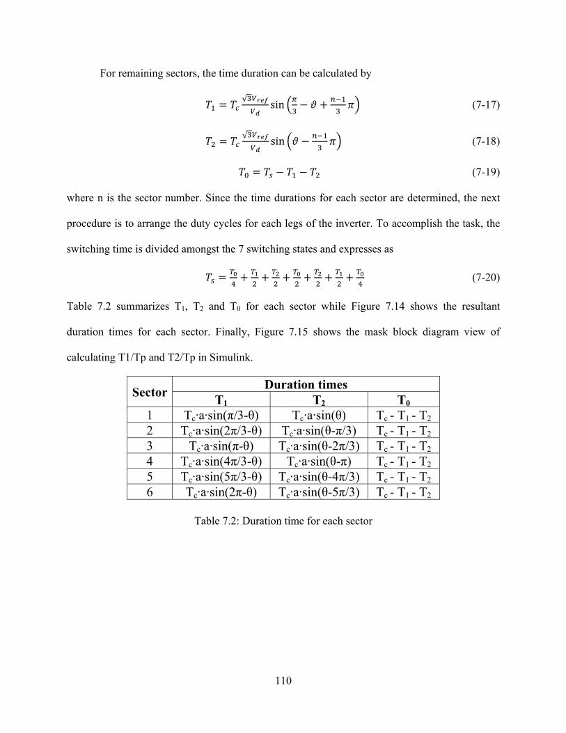
110

For remaining sectors, the time duration can be calculated by

√sin (7-17)

√sin (7-18)

(7-19)

where n is the sector number. Since the time durations for each sector are determined, the next

procedure is to arrange the duty cycles for each legs of the inverter. To accomplish the task, the

switching time is divided amongst the 7 switching states and expresses as

(7-20)

Table 7.2 summarizes T1, T2 and T0 for each sector while Figure 7.14 shows the resultant

duration times for each sector. Finally, Figure 7.15 shows the mask block diagram view of

calculating T1/Tp and T2/Tp in Simulink.

Sector Duration times

T1 T2 T0 1 Tc·a·sin(π/3-θ) Tc·a·sin(θ) Tc - T1 - T2 2 Tc·a·sin(2π/3-θ) Tc·a·sin(θ-π/3) Tc - T1 - T2 3 Tc·a·sin(π-θ) Tc·a·sin(θ-2π/3) Tc - T1 - T2 4 Tc·a·sin(4π/3-θ) Tc·a·sin(θ-π) Tc - T1 - T2 5 Tc·a·sin(5π/3-θ) Tc·a·sin(θ-4π/3) Tc - T1 - T2 6 Tc·a·sin(2π-θ) Tc·a·sin(θ-5π/3) Tc - T1 - T2

Table 7.2: Duration time for each sector

111

Figure 7.14: Waveform showing sequence of switching states for each sector [43]

112

Figure 7.15: Calculation of T1/Tp and T2/Tp block

7.4 Hardware Setup

Before examining the hardware setup, note that the steps do not have to be followed these

steps, but could start differently. The following procedures were used to conduct the hardware

test.

1. Connect the banana plug cables to the positive (7) and negative (N) of variable DC power

supply, (Labvolt 8821-20) with the positive and negative terminals of the digital

multimeter. If the designated power supply is not present, using alternative power supply

that meets the voltage and current rating can be used.

2. Connect the positive (7) and negative terminal (N) of the power supply to the positive (1

or +HV) and negative terminal (2 or GND) of the inverter. Then, connect the positive and

negative terminal of the inverter with the positive and negative terminal of E9.

3. Then, connect the three current outputs (3, 4, and 5 of IGBT or Phase A1, B1, and C1 of

MOSFET) of inverter with the positive terminals (I9, I10, and I11) of the current

113

measurement of the data acquisition (OP8660). The reason I9, I10, and I11 terminals

were used is the connection on back side of the data acquisition with the analog output

[39]. In other words, I1, I2, and I3 or others can be used if the connection on the back

side is connected as instructed in [39].

4. Link the negative terminals of I9, I10, and I11 with the ABC terminals of the motor from

Figure 7.8.

5. By using BNC cable, connect ADCH17 through 20 with the terminal 1, 2, 3, and 5 of

OP8660 Analog Outputs, where ADCH17 through 19 are for three-phase currents while

ADCH20 is for DC-link voltage.

6. Connect DB9 cable between Lab-volt IGBT inverter board and Slave I/O port of

dSPACE board to send PWM signals.

7. Connect between INC1 and encoder terminal of the motor to measure the rotor position.

8. Adjust the shaft of the PM motor to d-axis. This can be adjusted by using simple small

DC power supply. To accomplish the task, connect the positive terminal of power supply

to A-phase while negative terminal to B-phase. Increase the voltage little bit. Be cautious

while you are increasing the voltage.

7.5 Results

Three tests were conducted to observe the effect: acceleration and deceleration test, load

torque test, and flux weakening control test. Since the motor parameter varies automatically as

the motor operates, separate parameter variation test wasn’t conducted. Unlike in the simulation,

in order to observe the impact of the controller, each test was demonstrated individually. 15 kHz

114

with 0.1 μs dead-time and 0.1 ms were used for the switching frequency and sampling rate,

respectively.

7.5.1 Acceleration and Deceleration Test

At t=0.76 s, the input speed was increased from 0 rad/sec to 100 rad/sec, and then stayed

at 100 rad/sec for a second. At t=1.76s, the speed was decreased to 50 rad/sec and kept its value

for a second. At t=2.76 s, the speed was increased to 200 rad/sec and decreased again to 100

rad/sec at t=3.76 s.

Figure 7.16 and 7.17 show the speed and dq current traction of both proposed and

conventional controller. As it illustrates, both controller performed similarly. On the other hand,

a significant difference was observed in the voltage magnitude graph as illustrated in Fig. 7.18.

When the speed was increased from 50 rad/s to 200 rad/s, the conventional controller was

produced the peak voltage magnitude of 1.12 while the ANN controller produced 1.02. This

means that the ANN controller is more efficient than the conventional controller when the motor

is accelerating, since the voltage is proportional to current.

115

Figure 7.16: Speed traction of SPMSM (hardware)

Figure 7.17: Dq-axis current traction of SPMSM (hardware)

0 0.5 1 1.5 2 2.5 3 3.5 4 4.5 50

20

40

60

80

100

120

140

160

180

200

Time (s)

Spe

ed (

rad/

s)

Reference

ANNConventional

0 0.5 1 1.5 2 2.5 3 3.5 4 4.5 5-4

-2

0

2

4

6

8

Time (s)

Cur

rent

(A

)

Id ANN Iq ANN Id conventional Iq conventional

3.08 3.1 3.12 3.14 3.16 3.18 3.2 3.22

190

195

200

205

116

Figure 7.18: Vm of SPMSM (hardware)

7.5.2 Load Torque Variation Test

Load torque was applied by connecting 56.14 Ω resistor across the terminal of

DCGEN7105 motor/generator while the PM motor was rotating 200 rad/s. The purpose of this

resistor is to form close-loop circuit in the stator, so the current can be flow through the stator of

DCGEN7105 motor. The concept of Faraday’s law of induction is applied to accomplish the task.

For example, the rotating rotor while no current flows through the stator causes the back-EMF to

be induced across the stator of the generator. By Ohm’s law, if a resistor is connected between

terminals, a close-loop circuit is created. Then, this current will generate the opposing magnetic

field against the back-EMF. Thus, certain load torque will be created. The resistance of 56.14 Ω

was selected because it was the lowest resistance that could be found in the lab. As a result, when

this resistance was applied, 0.32 A of current was flowed through the stator winding.

0 0.5 1 1.5 2 2.5 3 3.5 4 4.5 50

0.2

0.4

0.6

0.8

1

1.2

1.4

Time (s)

Vm

(un

itles

s)

ANNConventional

3 3.1 3.2 3.3 3.4

0.8

0.85

0.9

0.95

1

1.05

1.1

117

Other solutions, such as controlling DCGEN7105 by applying the DC voltage across the

terminal and applying the friction manually, were considered and tried to apply it, but none of

mentioned solutions worked. The first approach couldn’t be implemented because the current

flows through the power supply coil and possibly burn the power supply. The second approach

was neglected because same amplitude of the friction and time could not be applied. Therefore,

connecting the resistor across the terminals was the only option to apply the load torque.

When the load torque was applied, only minimal impact was observed in both dq current

and speed. Thus, it is now shown in this thesis. Unlike them, the significant result was observed

in voltage magnitude graph. The result showed that the proposed controller is utilizing less

voltage than the conventional controller. As Fig. 7.19 shows, the voltage magnitude of the

proposed controller was 0.05 in average less than the conventional controller.

Figure 7.19: Load torque Vm traction of SPMSM

0 0.5 1 1.5 2 2.5 3 3.5 4 4.5 50.83

0.84

0.85

0.86

0.87

0.88

0.89

0.9

Vm

(un

itles

s)

Conventional

ANN

118

7.5.3 Flux Weakening Control Test

At t=0.5 s, the input speed was increased from 0 rad/s to 200 rad/s with slope of 200

rad/s2. As soon as the speed reaches 200 rad/s, the slope was decreased to 10 rad/s2 until it

reaches 280 rad/s. Then, the input speed was kept for 4 seconds and decreased to 100 rad/s.

Fig. 7.23 represents the speed traction of both controllers. It clearly shows that the

conventional controller cannot track the speed reference while the proposed controller can.

Further, Fig 7.21 shows that while the proposed controller used the flux weakening method by

preventing the voltage magnitude to exceed 1.2, which is maximum voltage magnitude that the

motor can achieve, the conventional controller could not. Fig. 7.22 shows the reference d-axis

current of both controllers while Fig 7.23 shows the actual dq current tractions. Due to cable and

other noise, the actual dq currents were hard to comprehend. However, the reference d-axis that

is shown in Fig 7.23 shows that the flux weakening control works well in the proposed controller

while not in the conventional controller.

Figure 7.20: a) Conventional and b) ANN speed traction of SPMSM

0 5 10 15 200

50

100

150

200

250

300

Time (s)

Spe

ed (

rad/

s)

Reference

Conventional

0 5 10 15 200

50

100

150

200

250

300

Time (s)

Spe

ed (

rad/

s)

Reference

ANN

a) b)

119

Figure 7.21: a) Conventional and b) ANN voltage magnitude of SPMSM

Figure 7.22: a) Conventional and b) ANN d-axis reference current of SPMSM

Figure 7.23: a) Conventional and b) ANN actual dq current traction of SPMSM

0 5 10 15 200

2

4

6

8

10

Time (s)

Vm

(un

itles

s)

0 5 10 15 200

0.2

0.4

0.6

0.8

1

1.2

1.4

Time (s)

Vm

(un

itles

s)

0 5 10 15 20-20

-15

-10

-5

0

Time (s)

Cur

rent

(A

)

0 5 10 15 20-0.5

-0.4

-0.3

-0.2

-0.1

0

Time (s)

Cur

rent

(A

)

0 5 10 15 20-30

-20

-10

0

10

20

Time (s)

Cur

rent

(A

)

Id conventional

Iq conventional

0 5 10 15 20-4

-2

0

2

4

6

Time (s)

Cur

rent

(A

)

Id ANN Iq ANN

a) b)

a) b)

a) b)

120

CHAPTER 8

CONCLUSION

In this thesis, the artificial neural network based vector control for PMSMs has been

evaluated by theoretical analysis, simulation, hardware experiment, and comparison with

conventional PI-based vector control.

First, the background of the PMSM and other control schemes from other literature were

discussed. Through the background search, the PMSM was widely used in applications that need

precise and intricate operation and possessed many advantages like high torque density, high

efficiency, and others compared to other AC machines. Four other control schemes, such as H∞,

fuzzy logic, matrix inverter fed, and wavelet neural network, were observed. Except few control

schemes, most literatures validated their control in only simulation, not hardware experiment.

This inspired the author to investigate the control scheme that can function in both simulation

and real world.

Second, this thesis included the detailed explanations of the motor parameters that are

required by the control. Those parameters are stator resistance, inductances, flux linkage constant,

inertia, and more. The investigation covered not only the backgrounds of each parameter, but

also how to measure the parameters.

In following section, the conventional PI-based field oriented and novel neural network

vector controllers were investigated. In each subsection, both the mathematical representation

121

and Simulink model were presented. In addition, in neural network section, detailed training

mechanisms with examples were covered.

Chapter 4 summarized the MTPA and flux weakening control. The fundamentals and

various control schemes of MTPA and flux weakening were explained in detail.

Then, in Chapter 5, this thesis discussed the electric model that was constructed by the

author. The electric model was comprised of four major blocks: Driver, Motor drive, Shaft and

Differential, and Vehicle dynamics with chassis, tire, and mechanical brake.

Then, the motor and controllers were simulated using MATLAB/Simulink. To observe

the effectiveness of the proposed control, it was compared with the conventional PI-based

control. The power rating of SPMSM and IPMSM was 0.2 kW and 100 kW, respectively. 0.2

kW SPMSM was chosen to compare the result of the hardware motor while 100 kW IPMSM was

selected to validate the effectiveness of the proposed control in electric vehicle application. Both

SPMSM and IPMSM were observed when the motor is 1) accelerating and decelerating, 2)

experiencing varying load torque, 3) experiencing varying parameter, and 4) performing the flux

weakening control. First, for SPMSM, the proposed control sustained its operation very stably

and reliably in the flux weakening region, but the conventional PI-based control could not keep

the operation. Second, for IPMSM, the result showed that the NN control utilizes less d-axis

current than the conventional controller. This conveys that the NN control has less susceptible

for the magnet to be demagnetized. Lastly, the proposed control was demonstrated in electric

vehicle model. The result showed that the proposed controller can be a potential replacement of

the existing control scheme, such as PID, fuzzy logic, or etc, and provides adequate traction

control in EV application.

122

Finally, this thesis conducted the hardware experiment to verify the proposed control in

real environment. 200 W BLDC motor from Motorsolver and dSPACE CP1103 controller were

utilized. For clear clarification, this thesis included individual instructions how the hardware

experiment was setup. As similar with the simulation, the proposed control was compared with

the conventional controller. Three tests were considered and are acceleration and deceleration

test, load torque variation test, and flux weakening control test. Like in the simulation, the

proposed control performed better in flux weakening region than the conventional control. Even

though the proposed control could perform the flux weakening control well, the PI-based

controller could not. Further, there was 3.5% increase improvement in maximum speed when the

proposed control is used.

8.1 Limitation and Future Work

The major limitation of this work was ignoring the non-linearity and saturation of

magnetic materials, including stator and rotor saturation. If these are accounted, the complex

control is required. Another limitation is lacking the validation result of IPMSM in hardware.

Because the lab did not have any IPMSM motor, this couldn’t be conducted. Thus, the future

goal is conducting the hardware test for IPMSM and validating the effectiveness of the proposed

control.

123

REFERENCES

[1] T. Lee, C. Lin, and F. Lin, “An Adaptive H∞ Controller Design for Permanent Magnet Synchronous Motor Drives,” Control Engineering Practice 13, pp. 425-439, 2005.

[2] A. Mishra, V. Mahajan, P. Agarwal, and S.P. Srivastava, “Fuzzy Logic Based Speed and Current Control of Vector Controlled PMSM Drive,” 2012 2nd International Conf. on Power, Ctrl, and Embedded Sys, 2012.

[3] Microchip Technology, “Permanent Magnet Synchronous Motor (PMSM),” Microchip Technology, Recordal No. 090049794, 1998. [Online]. Available: http://www.microchip.com/design-centers/motor-control-and-drive/motor-types/pmsm [Accessed: Mar. 6, 2016].

[4] H. Poesch, “Permanent magnet motors outperform induction motors in many applications,”Control Engineering, Sept. 24, 2012. [Online]. Available: http://www.controleng.com/single-article/permanent-magnet-motors-outperform-induction-motors-in-many-applications/413305407b2989675983a5babac0ac6d.html. [Accessed: Mar. 6, 2016].

[5] Toyota, “Toyota 2016 Prius,” Toyota, [Online]. Available: http://www.toyota.com/prius/features.html#!/mechanical_performance/1223/1225/1228/ 1227. [Accessed: Mar. 6, 2016].

[6] Tesla, “Tesla Model S 2016,” Tesla, [Online]. Available: http://www.teslamotors.com/support/model-s-specifications. [Accessed: Mar. 6, 2016].

[7] Hyundai, “2016 Sonata Hybrid SE,” Hyundai, [Online]. Available: https://www.hyundaiusa.com/sonata-hybrid/specifications.aspx. [Accessed: Mar. 6, 2016].

[8] Nissan, “2016 Leaf EV,” Nissan, [Online]. Available: http://www.nissanusa.com/electric-cars/leaf/versions-specs. [Accessed: Mar. 6, 2016].

[9] Honda, “2016 Accord Hybrid,” Honda, [Online]. Available: http://automobiles.honda.com/accord-hybrid/specifications.aspx. [Accessed: Mar. 6, 2016].

[10] S. Li, T.A. Haskew, and L. Xu, “Conventional and Novel Control Designs for Direct Driven PMSG Wind Turbines,” Electric Power System Research, vol. 80, pp. 328-338, March 2010.

[11] H. Kamel, H. Hasanien, and H. Ibrahim, “Speed Control of PMSM using Fuzzy Logic Controller,” Electric Machines and Drives Conf., pp. 1587-1591, 2009.

124

[12] H. Lu, and M. Chang, “Online Speed Control of PMSM using Self-constructing Recurrent Fuzzy Neural Network,” 2008 Int. Conf. on Machine Learning and Cyber., vol. 7, pp. 3857 – 3862, 2008.

[13] C. Xia, J. Zhao, Y. Yan, and T. Shi, “A Novel Direct Torque and Flux Control Method of Matrix Converter-Fed PMSM Drives,”IEEE Trans. on Power Electron., vol. 29(10), pp. 5417-5430, 2014.

[14] M. Khan, M. Uddin, and M. Rahman, “A Novel Wavelet-Neural Network-Based Robust Controller for IPM Motor Drives,” IEEE Trans. Ind. Appl., vol. 49(5), pp. 2341-2351, Sep./Oct. 2013.

[15] J. Moreno, M. E. Ortuzar, and J. W. Dixon, “Energy-management system for a hybrid electric vehicle, using ultracapacitors and neural networks,” IEEE Trans. on Ind. Electron., vol. 53(2), pp. 614-623, Apr. 2006.

[16] Z. Chen, C. C. Mi, J. Xu, X. Gong, and C. You, “Energy management for a power-split plug-in hybrid electric vehicle based on dynamic programming and neural networks,” IEEE Trans. on Veh. Tech., vol. 51(3), pp. 2321-2330, Oct. 2014.

[17] D. C. Giancoli, Physic, 4th ed., Prentice Hall, 1995.

[18] V. Bobek, “PMSM Electrical Parameters measurement,” Freescale Semiconductor, AN4680, 2013.

[19] G. Dajaku and D. Gerling, “Design of Permanent Magnet Machines for Hybrid Vehicles,” ANSYS Conference & 25th CADFEM Users’ Meeting 2007, pp. 1-7, Nov. 21-23, 2007.

[20] J. Hendershot and T. Miller, “Design of Brushless PM machines,” Motor Design Books LLC, 2010.

[21] H. Hofmann and B. Hieb, “Characterizing and Validating a PMSM Model,”2012 MathWorks.

[22] MicroSemi, “Park, Inverse Park and Clarke, Inverse Clarke Transformation MSS Software, MicroSemi.

[23] N. Mohan, “Advanced Electric Drives, Analysis, Control and Modeling using Simulink”, MNPERE, 2001.

[24] Opal-RT Technologies, “RT-Events,” OPAL-RT Technologies. [Online]. Available: www.opal-rt.com\node\292. [Accessed: Mar 6, 2016].

[25] S.N. Balakrishnan and V. Biega, “Adaptive-critic-based neural networks for aircraft optimal control,” Journal of Guidance, Control, and Dyanmic, vol. 19 (4), pp. 893-898, Jul./Aug. 1996.

125

[26] G. K. Venayagamoorthy, R. G. Harley, and D. C. Wunsch, “Comparison of heuristic dynamic programming and dual heuristic programming adaptive critics for neurocontrol of a turbogenerator,” IEEE Trans. Neural Netw., vol. 13(3), pp. 764-773, May 2002.

[27] S. Li, M. Fairbank, X. Fu, D. C. Wunsch, and E. Alonso, “Nested-Loop Neural Network for Control of a Grid-Connected Rectifier/Inverter under Disturbance, Dynamic and Power Converter Switching Conditions,” IEEE Trans. on Neural Networks and Learning Systems, vol. 25(4), pp. 738-750, 2014.

[28] L. Art and H. Mauch, “Dynamic Programming,” Springer vol.38, 2007.

[29] A. J. Wood, B. F. Wollenberg, G. B. Sheble, “Power Generation, Operation, and Control,” John Wiley & Sons 2014.

[30] M. A. Lourakis, “A Brief Descriptions of the Levenberg-Marquardt Algorithm Implemented by levmar,” matrix, vol. 3, p. 2, 2005.

[31] X. Fu and S. Li, “Training Recurrent Neural Networks with the Levenberg-Marquardt Algorithm for Optimal Control of a Grid-Connected Converter,” IEEE Trans. on Neural Netw.And Learning Syst., 2014.

[32] S. Jung, J. Hong, and K. Nam, “Current Minimizing Torque Control of the IPMSM using Ferrari’s Method,” IEEE Trans. On Power Electron., vol. 28(12), Dec, 2013.

[33] D. Fita, “Field Weakening Control of PMSM,” M. S. thesis, Dept. Elect. Eng., Addis Ababa Univ., Kebena, Ethiopia, 2005.

[34] Parker, “Electric and Hybrid Vehicle, Accessory, Power Generation & Traction Motor Solutions,” GVM210-150 datasheet, 2014.

[35] Rinehart Motion Systems LLC, “AC Motor Controller for Electric and Hybrid Vehicles,” PM Family datasheet, Jan. 2012.

[36] A123, “Energy Core Pack (23kWh),” A123. [Online]. Available: http://www.a123systems.com. [Accessed: Oct. 14, 2015].

[37] Kumho Tire, “ECSTA LX Platinum 215/55R17,” ECSTA LX Platinum datasheet.

[38] Pacejka, H.B. Tire and Vehicle Dynamics, Society of Automotive Engineers and Butterworth-Heinemann, Oxford, 2002.

[39] Tire (Magic Formula), MathWorks R2015b.

[40] M. Ehsani, Y. Gao, S. E. Gay, and A. Emadi, “Modern Electric, Hybrid Electric, and Fuel Cell Vehicles,” CRCPress LLC, 2005.

[41] K. Miller-Wilson, “List of Car Weights,” LovetoKnow. [Online]. Available: car.lovetoknow.com/List_of_Car_Weights. [Accessed: Mar. 3, 2016].

126

[42] OPAL-RT, “OP8660 HIL Controller User Guide”, OP8660 HIL datasheet, Oct. 2012.

[43] B. Tolunay, “SVPWM for Three-level converters, a Labview Implementation,” M. S. thesis, Dept. of Elec. Eng., Uppsala University, Uppsala, Sweden, 2012.