thesis proposal - carnegie mellon school of …zichaoy/proposal.pdf · december 11, 2017 draft ules...

December 11, 2017DRAFT

Thesis ProposalIncorporating Structural Bias into Neural

NetworksZichao Yang

Dec 2017

School of Computer ScienceCarnegie Mellon University

Pittsburgh, PA 15213

Thesis Committee:Eric Xing (co-chair)

Taylor Berg-Kirkpatrick (co-chair)Alexander Smola

Ruslan SalakhutdinovLi Deng (Citadel)

Submitted in partial fulfillment of the requirementsfor the degree of Doctor of Philosophy.

Copyright c© 2017 Zichao Yang


AbstractThe rapid progress in artificial intelligence in recent years can largely be at-

tributed to the resurgence of neural networks, which enables learning representa-tions in an end-to-end manner. Although neural network are powerful, they havemany limitations. For examples, neural networks are computationally expensive andmemory inefficient; Neural network training needs many labeled examples, espe-cially for tasks that require reasoning and external knowledge. The goal of this thesisis to overcome some of the limitations by designing neural network with structuralbias of the inputs taken into consideration.

This thesis aims to improve the efficiency of neural networks by exploring struc-tural properties of inputs in designing model architectures. Specifically, this thesisaugments neural networks with designed modules to improves their computationaland statistical efficiency. We instantiate those modules in a wide range of tasks in-cluding supervised learning and unsupervised learning and show those modules notonly make neural networks consume less memory, but also generalize better.


Contents

1 Introduction 1

I Structural Bias for Computational Efficiency 3

2 Learning Fast Kernels 42.1 Kernel Methods . . . . . . . . . . . . . . . . . . . . . . . . . . . . . . . . . . . 4

2.1.1 Basic Properties . . . . . . . . . . . . . . . . . . . . . . . . . . . . . . 42.1.2 Fastfood . . . . . . . . . . . . . . . . . . . . . . . . . . . . . . . . . . . 4

2.2 A la Carte . . . . . . . . . . . . . . . . . . . . . . . . . . . . . . . . . . . . . . 62.2.1 Gaussian Spectral Mixture Models . . . . . . . . . . . . . . . . . . . . . 62.2.2 Piecewise Linear Radial Kernel . . . . . . . . . . . . . . . . . . . . . . 72.2.3 Fastfood Kernels . . . . . . . . . . . . . . . . . . . . . . . . . . . . . . 9

2.3 Experiments . . . . . . . . . . . . . . . . . . . . . . . . . . . . . . . . . . . . . 9

3 Memory Efficient Convnets 123.1 The Adaptive Fastfood Transform . . . . . . . . . . . . . . . . . . . . . . . . . 12

3.1.1 Learning Fastfood by backpropagation . . . . . . . . . . . . . . . . . . 133.2 Deep Fried Convolutional Networks . . . . . . . . . . . . . . . . . . . . . . . . 143.3 Imagenet Experiments . . . . . . . . . . . . . . . . . . . . . . . . . . . . . . . 14

3.3.1 Fixed feature extractor . . . . . . . . . . . . . . . . . . . . . . . . . . . 153.3.2 Jointly trained model . . . . . . . . . . . . . . . . . . . . . . . . . . . . 16

II Structural Bias for Statistical Efficiency 17

4 Stacked Attention Networks 184.1 Stacked Attention Networks (SANs) . . . . . . . . . . . . . . . . . . . . . . . . 18

4.1.1 Image Model . . . . . . . . . . . . . . . . . . . . . . . . . . . . . . . . 184.1.2 Question Model . . . . . . . . . . . . . . . . . . . . . . . . . . . . . . . 194.1.3 Stacked Attention Networks . . . . . . . . . . . . . . . . . . . . . . . . 21

4.2 Experiments . . . . . . . . . . . . . . . . . . . . . . . . . . . . . . . . . . . . . 234.2.1 Data sets . . . . . . . . . . . . . . . . . . . . . . . . . . . . . . . . . . 234.2.2 Results . . . . . . . . . . . . . . . . . . . . . . . . . . . . . . . . . . . 23

iv


5 Reference-aware Language Models 255.1 Reference to databases . . . . . . . . . . . . . . . . . . . . . . . . . . . . . . . 255.2 Experiments . . . . . . . . . . . . . . . . . . . . . . . . . . . . . . . . . . . . . 28

5.2.1 Data sets . . . . . . . . . . . . . . . . . . . . . . . . . . . . . . . . . . 285.2.2 Results . . . . . . . . . . . . . . . . . . . . . . . . . . . . . . . . . . . 28

III Structural Bias for Unsupervised Learning 30

6 Variational Autoencoders for Text Modeling 316.1 Background on Variational Autoencoders . . . . . . . . . . . . . . . . . . . . . 316.2 Training Collapse with Textual VAEs . . . . . . . . . . . . . . . . . . . . . . . 326.3 Dilated Convolutional Decoders . . . . . . . . . . . . . . . . . . . . . . . . . . 336.4 Experiments . . . . . . . . . . . . . . . . . . . . . . . . . . . . . . . . . . . . . 34

6.4.1 Data sets . . . . . . . . . . . . . . . . . . . . . . . . . . . . . . . . . . 346.4.2 Results . . . . . . . . . . . . . . . . . . . . . . . . . . . . . . . . . . . 35

7 Proposed work 377.1 Unsupervised Natural Language Learning . . . . . . . . . . . . . . . . . . . . . 377.2 Timeline . . . . . . . . . . . . . . . . . . . . . . . . . . . . . . . . . . . . . . . 37

Bibliography 38

v


Chapter 1

Introduction

Over the past decades, machine learning models have relied heavily on hand-crafted features tolearn well. With the recent breakthrough of neural networks in computer vision [21] and naturallanguage processing [40], feature representations can be learned directly in an end-to-end man-ner. Minimum human efforts are required to preprocess the data and neural network models aredirectly resorted to optimize learning the feature representation. Although neural networks arepowerful, they still have many limitations. On the one hand, neural networks are computation-ally expensive and memory inefficient. They can have hundreds of millions of parameters and amodel can take several GBs. On the other hand, neural networks, though with large representa-tion capacity, require many labeled examples to work well. This is especially true for tasks thatrequire reasoning and external knowledge, which are two key components in human intelligence.The goal of this thesis is to overcome some of the limitations by designing neural networks withstructural bias taken into consideration. Designing neural network according to characteristics ofthe inputs reduces the capacity of hypothesis space, this not only reduces the memory footprintof neural networks, but also make neural networks learn more efficiently and generalize better.

This thesis is composed of three parts:

• Incorporating Structural Bias for Computational Efficiency: Fully connected layerin neural networks are computational expensive and memory inefficient. Reducing thenumber of parameters would improve the efficiency of neural networks and facilitate itsdeployment on embedded devices. In this part of thesis, we propose to replace the fullyconnected layers with an adaptive Fastfood transform, which is a generalization of theFastfood transform for approximating random features in kernels. We first begin by veri-fying the expressiveness of Fastfood transform in the context of kernel methods in Chapter2. This part is largely based on work from [47]. We then embed the Fastfood transformin neural networks to replace fully connected layers to show that it can not only reducethe number of parameters but also has sufficient representation capacity. This part of workappears in Chapter 3 and is largely based on the work from [46].

• Incorporating Structural Bias for Statistical Efficiency: Neural network training needsmany labeled examples. This is especially true for more advanced tasks that require reason-ing and external knowledge, in which labeled examples are more expensive to get. Simpleneural network models are not sufficient and it is necessary to design more efficient mod-

1


ules to accomplish these goals. In this part of the thesis, we augment neural networks withmodules that support reasoning and querying external knowledge. We instantiate thosemodels in the context of visual question answering (Chapter 4) and dialogue modeling(Chapter 5). In Chapter 4, we propose a stacked attention network to support multiplestep reasoning to find the clues to the answer given an image and question. This chapteris largely based on the work from [49]. In Chapter 5, we study task oriented dialoguemodeling. A dialogue model has to make the right recommendation based on an externaldatabase according to users’ query. We augment a standard sequence to sequence modelwith a table pointer module to enable searching the table in replying users’ query. Thischapter is largely based on the work from [48]. We show models with those modules learnmore efficiently and generalize better in those tasks.

• Incorporating Structural Bias for Unsupervised Learning: Incorporating structuralbias is also helpful for unsupervised learning. In Chapter 6, we investigate the variationalauto-encoder for text modeling. Previous work has found that LSTM-VAE tends to ignorethe information from the encoder and the VAE collapses to a language model. We pro-pose to use a dilated CNN as the decoder, with which we can control the explicit trade offbetween contextual capacity of decoders and efficient use of encoding information, thusavoiding the training collapse problem observed in previous works. This chapter is largelybased on the work from [51].

2


Part I

Structural Bias for ComputationalEfficiency

3


Chapter 2

Learning Fast Kernels

2.1 Kernel Methods

2.1.1 Basic PropertiesDenote by X the domain of covariates and by Y the domain of labels. Moreover, denote X :={x1, . . . , xn} and Y := {y1, . . . , yn} data drawn from a joint distribution p over X × Y . Finally,let k : X × X → R be a symmetric positive semidefinite kernel [28], such that every matrix Kwith entries Kij := k(xi, xj) satisfies K � 0.

The key idea in kernel methods is that they allow one to represent inner products in a high-dimensional feature space implicitly, using

k(x, x′) = 〈φ(x), φ(x′)〉 . (2.1)

While the existence of such a mapping φ is guaranteed by the theorem of Mercer [28], manipu-lation of φ is not generally desirable since it might be infinite dimensional. Instead, one uses therepresenter theorem [19, 35] to show that when solving regularized risk minimization problems,the optimal solution f(x) = 〈w, φ(x)〉 can be found as linear combination of kernel functions:

〈w, φ(x)〉 =

⟨n∑i=1

αiφ(xi), φ(x)

⟩=

n∑i=1

αik(xi, x).

While this expansion is beneficial for small amounts of data, it creates an unreasonable burdenwhen the number of datapoints n is large. This problem can be overcome by computing approx-imate expansions.

2.1.2 FastfoodThe key idea in accelerating 〈w, φ(x)〉 is to find an explicit feature map such that k(x, x′) can beapproximated by

∑mj=1 ψj(x)ψj(x

′) in a manner that is both fast and memory efficient. Followingthe spectral approach of Rahimi and Recht [31], we exploit that for translation invariant kernelsk(x, x′) = κ(x− x′) we have

k(x, x′) =

∫ρ(ω) exp (i 〈ω, x− x′〉) dω . (2.2)

4


Here ρ(ω) = ρ(−ω) ≥ 0 to ensure that the imaginary parts of the integral vanish. Without loss ofgenerality we assume that ρ(ω) is normalized, e.g. ‖ρ‖1 = 1. A similar spectral decompositionholds for inner product kernels k(x, x′) = κ(〈x, x′〉) [23, 34].

Rahimi and Recht [31] suggested to sample from the spectral distribution ρ(ω) for a MonteCarlo approximation to the integral in (2.2). For example, the Fourier transform of the popularGaussian kernel is also Gaussian, and thus samples from a normal distribution for ρ(ω) can beused to approximate a Gaussian (RBF) kernel.

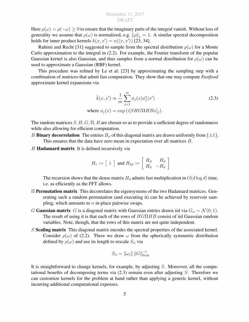
This procedure was refined by Le et al. [23] by approximating the sampling step with acombination of matrices that admit fast computation. They show that one may compute Fastfoodapproximate kernel expansions via

k(x, x′) ∝ 1

m

m∑j=1

φj(x)φ∗j(x′) (2.3)

where φj(x) = exp (i[SHGΠHBx]j) .

The random matrices S,H,G,Π, B are chosen so as to provide a sufficient degree of randomnesswhile also allowing for efficient computation.B Binary decorrelation The entriesBii of this diagonal matrix are drawn uniformly from {±1}.

This ensures that the data have zero mean in expectation over all matrices B.

H Hadamard matrix It is defined recursively via

H1 :=[

1]

and H2d :=

[Hd Hd

Hd −Hd

]The recursion shows that the dense matrixHd admits fast multiplication inO(d log d) time,i.e. as efficiently as the FFT allows.

Π Permutation matrix This decorrelates the eigensystems of the two Hadamard matrices. Gen-erating such a random permutation (and executing it) can be achieved by reservoir sam-pling, which amounts to n in-place pairwise swaps.

G Gaussian matrix G is a diagonal matrix with Gaussian entries drawn iid via Gii ∼ N (0, 1).The result of using it is that each of the rows of HGΠHB consist of iid Gaussian randomvariables. Note, though, that the rows of this matrix are not quite independent.

S Scaling matrix This diagonal matrix encodes the spectral properties of the associated kernel.Consider ρ(ω) of (2.2). There we draw ω from the spherically symmetric distributiondefined by ρ(ω) and use its length to rescale Sii via

Sii = ‖ωi‖ ‖G‖−1Frob

It is straightforward to change kernels, for example, by adjusting S. Moreover, all the compu-tational benefits of decomposing terms via (2.3) remain even after adjusting S. Therefore wecan customize kernels for the problem at hand rather than applying a generic kernel, withoutincurring additional computational expenses.

5


2.2 A la CarteIn keeping with the culinary metaphor of Fastfood, we now introduce a flexible and efficientapproach to kernel learning a la carte. That is, we will adjust the spectrum of a kernel in sucha way as to allow for a wide range of translation-invariant kernels. Note that unlike previousapproaches, this can be accomplished without any additional cost since these kernels only differin terms of their choice of scaling.

In Random Kitchen Sinks and Fastfood, the frequencies ω are sampled from the spectral den-sity ρ(ω). One could instead learn the frequencies ω using a kernel learning objective function.Moreover, with enough spectral frequencies, such an approach could learn any stationary (trans-lation invariant) kernel. This is because each spectral frequency corresponds to a point mass onthe spectral density ρ(ω) in (2.2), and point masses can model any density function.

However, since there are as many spectral frequencies as there are basis functions, individu-ally optimizing over all the frequencies ω can still be computationally expensive, and susceptibleto over-fitting and many undesirable local optima. In particular, we want to enforce smoothnessover the spectral distribution. We therefore also propose to learn the scales, spread, and locationsof groups of spectral frequencies, in a procedure that modifies the expansion (2.3) for fast kernellearning. This procedure results in efficient, expressive, and lightly parametrized models.

2.2.1 Gaussian Spectral Mixture ModelsFor the Gaussian Spectral Mixture kernels of Wilson and Adams [44], translation invarianceholds, yet rotation invariance is violated: the kernels satisfy k(x, x′) = k(x+δ, x′+δ) for all δ ∈Rd; however, in general rotations U ∈ SO(d) do not leave k invariant, i.e. k(x, x′) 6= k(Ux, Ux′).These kernels have the following explicit representation in terms of their Fourier transform F [k]

F [k](ω) =∑q

v2q

2[χ (ω, µq,Σq) + χ (−ω, µq,Σq)]

where χ(ω, µ,Σ) =e−

12

(µ−ω)>Σ−1(µ−ω)

(2π)d2 |Σ| 12

In other words, rather than choosing a spherically symmetric representation ρ(ω) as typical for(2.2), Wilson and Adams [44] pick a mixture of Gaussians with mean frequency µq and vari-ance Σq that satisfy the symmetry condition ρ(ω) = ρ(−ω) but not rotation invariance. By thelinearity of the Fourier transform, we can apply the inverse transform F−1 component-wise toobtain

k(x− x′) =∑q

v2q

|Σq|12

(2π)d2

exp

(−1

2

∥∥∥Σ12q (x− x′)

∥∥∥2)

cos 〈x− x′, µq〉 (2.4)

Lemma 1 (Universal Basis) The expansion (2.4) can approximate any translation-invariant ker-nel by approximating its spectral density.

6


Proof This follows since mixtures of Gaussians are universal approximators for densities [38],and by the Fourier-Plancherel theorem, approximation in the Fourier domain amounts to approx-imation in the original domain.Note that the expression in (2.4) is not directly amenable to the fast expansions provided byFastfood since the distributions are shifted. However, a small modification allows us to efficientlycompute kernels of the form of (2.4). The key insight is that shifts in Fourier space by ±µq areaccomplished by multiplication by exp (±i 〈µq, x〉). Here the inner product can be precomputed,

which costs only O(d) operations. Moreover, multiplications by Σ− 1

2q induce multiplication by

Σ12q in the original domain, which can be accomplished as preprocessing. For diagonal Σq the

cost is O(d).In order to preserve translation invariance we compute a symmetrized set of features. We have

the following algorithm (we assume diagonal Σq — otherwise simply precompute and scale x):Preprocessing — Input m, {(Σq, µq)}for each q generate random matrices Sq, Gq, Bq,Πq

Combine group scaling Bq ← BqΣ12q

Feature Computation — Input S,G,B,Π, µ,Σfor q = 1 to Q doζ ← 〈µq, x〉 (offset)ξ ← [SqHGqΠqHBqx] (Fastfood product)Compute features

φq·1 ← sin(ξ + ζ) and φq·2 ← cos(ξ + ζ)

and φq·3 ← sin(ξ − ζ) and φq·4 ← cos(ξ + ζ)

end forTo learn the kernel we learn the weights vq, dispersion Σq and locations µq of spectral fre-

quencies via marginal likelihood optimization, as described in section ??. This results in a kernellearning approach which is similar in flexibility to individually learning all md spectral frequen-cies and is less prone to over-fitting and local optima. In practice, this can mean optimizing overabout 10 free parameters instead of 104 free parameters, with improved predictive performanceand efficiency. See section 4.2 for more detail.

2.2.2 Piecewise Linear Radial KernelIn some cases the freedom afforded by a mixture of Gaussians in frequency space may be morethan what is needed. In particular, there exist many cases where we want to retain invarianceunder rotations while simultaneously being able to adjust the spectrum according to the data athand. For this purpose we introduce a novel piecewise linear radial kernel.

Recall (2.2) governs the regularization properties of k. We require ρ(ω) = ρ(‖ω‖) := ρ(r)for rotation invariance. For instance, for the Gaussian RBF kernel we have

ρ(‖ω‖2) ∝ ‖ω‖d−12 exp

(−‖ω‖

22

2

). (2.5)

For high dimensional inputs, the RBF kernel suffers from a concentration of measure problem[23], where samples are tightly concentrated at the maximum of ρ(r), r =

√d− 1. A fix is

7


ρi(r)

ri-1

1

ri ri+1

ρ(r) =∑i

αiρi(r)

||ω||r0 r1 r2 r3 r4

α1

α2

α3

Figure 2.1: Piecewise linear functions. Top: single basis function. Bottom: linear combinationof three functions. Additional degrees of freedom are fixed by ρ(r0) = ρ(r4) = 0.

relatively easy, since we are at liberty to pick any nonnegative ρ in designing kernels. Thisprocedure is flexible but leads to intractable integrals: the Hankel transform of ρ, i.e. the radialpart of the Fourier transform, needs to be analytic if we want to compute k in closed form.

However, if we remain in the Fourier domain, we can use ρ(r) and sample directly fromit. This strategy kills two birds with one stone: we do not need to compute the inverse Fouriertransform and we have a readily available sampling distribution at our disposal for the Fastfoodexpansion coefficients Sii. All that is needed is to find an efficient parametrization of ρ(r).

We begin by providing an explicit expression for piecewise linear functions ρi such thatρi(rj) = δij with discontinuities only at ri−1, ri and ri+1. In other words, ρ(r) is a ‘hat’ functionwith its mode at ri and range [ri−1, ri+1]. It is parametrized as

ρi(r) := max

(0,min

(1,r − ri−1

ri − ri−1

,ri − rri+1 − ri

))By construction each basis function is piecewise linear with ρi(rj) = δij and moreover ρi(r) ≥ 0for all r.

Lemma 2 Denote by {r0, . . . , rn} a sequence of locations with ri > ri−1 and r0 = 0. Moreover,let ρ(r) :=

∑i αiρi(r). Then ρ(r) ≥ 0 for all r if and only if αi ≥ 0 for all i. Moreover, ρ(r)

parametrizes all piecewise linear functions with discontinuities at ri.

Now that we have a parametrization, we only need to discuss how to draw ω from ρ(‖ω‖) = ρ(r).We have several strategies at our disposal:• ρ(r) can be normalized explicitly via

ρ :=

∫ ∞0

ρ(r)dr =∑i

αi2(ri+1 − ri−1)

Since each segment ρi occurs with probability αi/(2ρ(ri+1− ri−1) we first sample the seg-ment and then sample from ρi explicitly by inverting the associated cumulative distributionfunction (it is piecewise quadratic).

• Note that sampling can induce considerable variance in the choice of locations. An alter-native is to invert the cumulative distribution function and pickm locations equidistantly atlocations i

m+ξ where ξ ∼ U [0, 1/m]. This approach is commonly used in particle filtering

8


[9]. We choose this strategy, since it is efficient yet substantially reduces the variance ofsampling.

The basis functions are computed as follows:Preprocessing(m,

{({αi}ni=1, {ri}n+1

i=0 ,Σ)}

)Generate random matrices G,B,ΠUpdate scaling B ← BΣ

12

Sample S from ρ(‖ω‖) as above

Feature Computation(S,G,B,Π)

φ1 ← cos([SHGΠHBx]) and φ2 ← sin([SHGΠHBx])

The rescaling matrix Σq is introduced to incorporate automatic relevance determination into themodel. Like with the Gaussian spectral mixture model, we can use a mixture of piecewiselinear radial kernels to approximate any radial kernel. Supposing there are Q components of thepiecewise linear ρq(r) function, we can repeat the proposed algorithm Q times to generate all therequired basis functions.

2.2.3 Fastfood KernelsThe efficiency of Fastfood is partly obtained by approximating Gaussian random matrices with aproduct of matrices described in section 2.1.2. Here we propose several expressive and efficientkernel learning algorithms obtained by optimizing the marginal likelihood of the data in Eq. (??)with respect to these matrices:FSARD The scaling matrix S represents the spectral properties of the associated kernel. For

the RBF kernel, S is sampled from a chi-squared distribution. We can simply change thekernel by adjusting S. By varying S, we can approximate any radial kernel. We learn thediagonal matrix S via marginal likelihood optimization. We combine this procedure withAutomatic Relevance Determination of Neal [30] – learning the scale of the input space –to obtain the FSARD kernel.

FSGBARD We can further generalize FSARD by additionally optimizing marginal likelihoodwith respect to the diagional matrices G and B in Fastfood to represent a wider class ofkernels.

In both FSARD and FSGBARD the Hadamard matrixH is retained, preserving all the computa-tional benefits of Fastfood. That is, we only modify the scaling matrices while keeping the maincomputational drivers such as the fast matrix multiplication and the Fourier basis unchanged.

2.3 ExperimentsWe evaluate the proposed kernel learning algorithms on many regression problems from the UCIrepository. We show that the proposed methods are flexible, scalable, and applicable to a largeand diverse collection of data, of varying sizes and properties. In particular, we demonstratescaling to more than 2 million datapoints (in general, Gaussian processes are intractable beyond104 datapoints); secondly, the proposed algorithms significantly outperform standard exact kernelmethods, and with only a few hyperparameters are even competitive with alternative methods that

9


involve training orders of magnitude more hyperparameters.1 All experiments are performed onan Intel Xeon E5620 PC, operating at 2.4GHz with 32GB RAM. Details such as initializationare in the supplement.

1 2 3 40.25

0.3

0.35

0.4

0.45

0.5

0.55

0.6

0.65

0.7

Q

RMSE

FARD

FSARD

GM

PWL

FSGBARD

SSGPR

(a) RMSE as a function of Q

0 2 4 6 8 10 12 14 16−0.2

0

0.2

0.4

0.6

0.8

1

1.2

1.4

training timeaccu

racy (

log

)

FRBF

FSARDFARD

GM

PWL

SSGPR

FSGBARD

(b) accuracy (log) vs training time

FRBF FARD FSARD GM PWL FSGBARD SSGPR

0

0.5

1

1.5

2

2.5

3

3.5

4

test

tim

e (

log

)

(c) test time (log) comparison

10 15 20 25 30 35 40 45 500.2

0.3

0.4

0.5

0.6

0.7

0.8

m

RMSE

FARD

FSARD

GM

PWL

FSGBARD

SSGPR

(d) RMSE as a function of m

0 2 4 6 8 10−0.2

0

0.2

0.4

0.6

0.8

1

1.2

1.4

RAM (log)

accu

racy (

log

)

FARD

FRBF

PWL

GM

FSARD

FSGBARDSSGPR

(e) accuracy (log) vs ram (log)

FRBF FARD FSARD GM PWL FSGBARD SSGPR RBF ARD−1

0

1

2

3

4

5

6

7

8

train

ing

tim

e (

log

)

(f) training time (log) comparison

Figure 2.2: Fig. 2.2a and Fig. 2.2d illustrate how RMSE changes as we vary Q and m on theSML dataset. For variable Q, the number of basis functions per group m is fixed to 32. Forvariable m the number of clusters Q is fixed to 2. FRBF and FARD are Fastfood expansionsof RBF and ARD kernels, respectively. Fig. 2.2b and Fig. 2.2e compare all methods in termsof accuracy, training time and memory. The accuracy score of a method on a given dataset iscomputed as accuracymethod = RMSEFRBF/RMSEmethod. For runtime and memory we take thereciprocal of the analogous metric, so that a lower score corresponds to better performance. Forinstance, timemethod = walltimemethod/walltimeFRBF. log denotes an average of the (natural) logscores, across all datasets. Fig. 2.2c and Fig. 2.2f compares all methods in terms of log test andtraining time (Fig. 2.2f also includes the average log training time for the exact ARD and RBFkernels across the smallest five medium datasets; these methods are intractable on any largerdatasets).

RBF and ARD On smaller datasets, with fewer than n = 2000 training examples, where exactmethods are tractable, we use exact Gaussian RBF and ARD kernels with hyperparameterslearned via marginal likelihood optimization. ARD kernels use Automatic Relevance De-termination [30] to adjust the scale of each input coordinate. Since these exact methods areintractable on larger datasets, we use Fastfood basis function expansions of these kernelsfor n > 2000.

1GM, PWL, FSARD, and FSGBARD are novel contributions of this paper, while RBF and ARD are popularalternatives, and SSGPR is a recently proposed state of the art kernel learning approach.

10


GM For Gaussian Mixtures we compute a mixture of Gaussians in frequency domain, as de-scribed in section 2.2.1. As before, optimization is carried out with regard to marginallikelihood.

PWL For rotation invariance, we use the novel Piecewise Linear radial kernels described insection 2.2.2. PWL has a simple spectral parametrization.

SSGPR Sparse Spectrum Gaussian Process Regression is a kitchen sinks (RKS) based modelwhich individually optimizes the locations of all spectral frequencies [? ]. We note thatSSGPR is heavily parametrized. Moreover, SSGPR is a special case of the proposed GMmodel if Q = m, and we set all GM bandwidths to 0 and weigh all terms equally.

FSARD and FSGBARD See section 2.2.3.

In Figures 2.2a we investigate how RMSE performance changes as we vary Q and m. TheGM and PWL models continue to increase in performance as more basis functions are used.This trend is not present with SSGPR or FSGBARD, which unlike GM and PWL, becomes moresusceptible to over-fitting as we increase the number of basis functions. Indeed, in SSGPR, andin FSGBARD and FSARD to a lesser extent, more basis functions means more parameters tooptimize, which is not true with the GM and PWL models.

We further investigate the performance of all seven methods, in terms of average normalisedlog predictive accuracy, training time, testing time, and memory consumption, shown in Figures2.2b and 2.2c (higher accuracy scores and lower training time, test time, and memory scores, cor-respond to better performance). Despite the reduced parametrization, GM and PWL outperformall alternatives in accuracy, yet require similar memory and runtime to the much less expressiveFARD model, a Fastfood expansion of the ARD kernel. Although SSGPR performs third best inaccuracy, it requires more memory, training time, testing runtime (as shown in Fig 2.2c), than allother models. FSGBARD performs similar in accuracy to SSGPR, but is significantly more timeand memory efficient, because it leverages a Fastfood representation. For clarity, we have so farconsidered log plots.

11


Chapter 3

Memory Efficient Convnets

3.1 The Adaptive Fastfood TransformLarge dense matrices are the main building block of fully connected neural network layers. Inpropagating the signal from the l-th layer with d activations hl to the l + 1-th layer with nactivations hl+1, we have to compute

hl+1 = Whl. (3.1)

The storage and computational costs of this matrix multiplication step are both O(nd). Thestorage cost in particular can be prohibitive for many applications.

Our proposed solution is to reparameterize the matrix of parameters W ∈ Rn×d with anAdaptive Fastfood transform, as follows

hl+1 = (SHGΠHB) hl = Whl. (3.2)

. The storage requirements of this reparameterization are O(n) and the computational cost isO(n log d). We will also show in the experimental section that these theoretical savings aremirrored in practice by significant reductions in the number of parameters without increasedprediction errors.

To understand these claims, we need to describe the component modules of the AdaptiveFastfood transform. For simplicity of presentation, let us first assume that W ∈ Rd×d. AdaptiveFastfood has three types of module:• S,G and B are diagonal matrices of parameters. In the original non-adaptive Fastfood

formulation they are random matrices, as described further. The computational and storagecosts are trivially O(d).

• Π ∈ {0, 1}d×d is a random permutation matrix. It can be implemented as a lookup table,so the storageand computational costs are also O(d).

• H denotes the Walsh-Hadamard matrix, which is defined recursively as

H2 :=

[1 11 −1

]and H2d :=

[Hd Hd

Hd −Hd

].

The Fast Hadamard Transform, a variant of Fast Fourier Transform, enables us to computeHdhl in O(d log d) time.

12


In summary, the overall storage cost of the Adaptive Fastfood transform is O(d), while thecomputational cost isO(d log d). These are substantial theoretical improvements over theO(d2)costs of ordinary fully connected layers.

When the number of output units n is larger than the number of inputs d, we can performn/d Adaptive Fastfood transforms and stack them to attain the desired size. In doing so, thecomputational and storage costs become O(n log d) and O(n) respectively, as opposed to themore substantialO(nd) costs for linear modules. The number of outputs can also be refined withpruning.

3.1.1 Learning Fastfood by backpropagationThe parameters of the Adaptive Fastfood transform (S,G and B) can be learned by standarderror derivative backpropagation. Moreover, the backward pass can also be computed efficientlyusing the Fast Hadamard Transform.

In particular, let us consider learning the l-th layer of the network, hl+1 = SHGΠHBhl.For simplicity, let us again assume that W ∈ Rd×d and that hl ∈ Rd. Using backpropagation,

assume we already have ∂E∂hl+1

, where E is the objective function, then

∂E

∂S= diag

{∂E

∂hl+1

(HGΠHBhl)>}. (3.3)

Since S is a diagonal matrix, we only need to calculate the derivative with respect to the diagonalentries and this step requires only O(d) operations.

Proceeding in this way, denote the partial products by

hS = HGΠHBhl

hH1 = GΠHBhl

hG = ΠHBhl

hΠ = HBhl

hH2 = Bhl. (3.4)

Then the gradients with respect to different parameters in the Fastfood layer can be computedrecursively as follows:

∂E

∂hS= S>

∂E

∂hl+1

∂E

∂hH1

= H>∂E

∂hS∂E

∂G= diag

{∂E

∂hH1

h>G

}∂E

∂hG= G>

∂E

∂hH1

∂E

∂hΠ

= Π>∂E

∂hG

∂E

∂hH2

= H>∂E

∂hΠ

∂E

∂B= diag

{∂E

∂hH2

h>l

}∂E

∂hl= B>

∂E

∂hH2

. (3.5)

Note that the operations in ∂E∂hH1

and ∂E∂hH2

are simply applications of the Hadamard transform,since H> = H, and consequently can be computed in O(d log d) time. The operation in ∂E

∂hΠ

13


is an application of a permutation (the transpose of permutation matrix is a permutation matrix)and can be computed in O(d) time. All other operations are diagonal matrix multiplications.

3.2 Deep Fried Convolutional Networks

Convolutional and pooling layers

Represent as a vector

FastFood

Softmax

Figure 3.1: The structure of a deep fried convolutional network. The convolution and poolinglayers are identical to those in a standard convnet. However, the fully connected layers arereplaced with the Adaptive Fastfood transform.

We propose to greatly reduce the number of parameters of the fully connected layers byreplacing them with an Adaptive Fastfood transform followed by a nonlinearity. We call thisnew architecture a deep fried convolutional network. An illustration of this architecture is shownin Figure 3.1.

In principle, we could also apply the Adaptive Fastfood transform to the softmax classifier.However, reducing the memory cost of this layer is already well studied; for example, [33]show that low-rank matrix factorization can be applied during training to reduce the size of thesoftmax layer substantially. Importantly, they also show that training a low rank factorizationfor the internal layers performs poorly, which agrees with the results of [8]. For this reason, wefocus our attention on reducing the size of the internal layers.

3.3 Imagenet ExperimentsWe now examine how deep fried networks behave in a more realistic setting with a much largerdataset and many more classes. Specifically, we use the ImageNet ILSVRC-2012 dataset whichhas 1.2M training examples and 50K validation examples distributed across 1000 classes.

We use the the Caffe ImageNet model1 as the reference model in these experiments [16]. Thismodel is a modified version of AlexNet [21], and achieves 42.6% top-1 error on the ILSVRC-2012 validation set. The initial layers of this model are a cascade of convolution and poolinglayers with interspersed normalization. The last several layers of the network take the form of anMLP and follow a 9216–4096–4096–1000 architecture. The final layer is a logistic regression

1https://github.com/BVLC/caffe/tree/master/models/bvlc_reference_caffenet

14

https://github.com/BVLC/caffe/tree/master/models/bvlc_reference_caffenet


layer with 1000 output classes. All layers of this network use the ReLU nonlinearity, and dropoutis used in the fully connected layers to prevent overfitting.

There are total of 58,649,184 parameters in the reference model, of which 58,621,952 arein the fully connected layers and only 27,232 are in the convolutional layers. The parametersof fully connected layer take up 99.9% of the total number of parameters. We show that theAdaptive Fastfood transform can be used to substantially reduce the number of parameters inthis model.

ImageNet (fixed) Error ParamsDai et al. [7] 44.50% 163MFastfood 16 50.09% 16.4MFastfood 32 50.53% 32.8MAdaptive Fastfood 16 45.30% 16.4MAdaptive Fastfood 32 43.77% 32.8MMLP 47.76% 58.6M

Table 3.1: Imagenet fixed convolutional layers: MLP indicates that we re-train 9216–4096–4096–1000 MLP (as in the original network) with the convolutional weights pretrained and fixed.Our method is Fastfood 16 and Fastfood 32, using 16,384 and 32,768 Fastfood features respec-tively. [7] report results of max-voting of 10 transformations of the test set.

3.3.1 Fixed feature extractorPrevious work on applying kernel methods to ImageNet has focused on building models onfeatures extracted from the convolutional layers of a pre-trained network [7]. This setting isless general than training a network from scratch but does mirror the common use case where aconvolutional network is first trained on ImageNet and used as a feature extractor for a differenttask.

In order to compare our Adaptive Fastfood transform directly to this previous work, we ex-tract features from the final convolutional layer of a pre-trained reference model and train anAdaptive Fastfood transform classifier using these features. Although the reference model usestwo fully connected layers, we investigate replacing these with only a single Fastfood transform.We experiment with two sizes for this transform: Fastfood 16 and Fastfood 32 using 16,384 and32,768 Fastfood features respectively. Since the Fastfood transform is a composite module, wecan apply dropout between any of its layers. In the experiments reported here, we applied dropoutafter the Π matrix and after the S matrix. We also applied dropout to the last convolutional layer(that is, before the B matrix).

We also train an MLP with the same structure as the top layers of the reference model forcomparison. In this setting it is important to compare against the re-trained MLP rather than thejointly trained reference model, as training on features extracted from fixed convolutional layerstypically leads to lower performance than joint training [52].

The results of the fixed feature experiment are shown in Table 3.1. Following [52] and [7]we observe that training on ImageNet activations produces significantly lower performance than

15


of the original, jointly trained network. Nonetheless, deep fried networks are able to outperformboth the re-trained MLP model as well as the results in [7] while using fewer parameters.

In contrast with our MNIST experiment, here we find that the Adaptive Fastfood transformprovides a significant performance boost over the non-adaptive version, improving top-1 perfor-mance by 4.5-6.5%.

3.3.2 Jointly trained modelFinally, we train a deep fried network from scratch on ImageNet. With 16,384 features in theFastfood layer we lose less than 0.3% top-1 validation performance, but the number of parametersin the network is reduced from 58.7M to 16.4M which corresponds to a factor of 3.6x. By furtherincreasing the number of features to 32,768, we are able to perform 0.6% better than the referencemodel while using approximately half as many parameters. Results from this experiment areshown in Table 3.2.

ImageNet (joint) Error ParamsFastfood 16 46.88% 16.4MFastfood 32 46.63% 32.8MAdaptive Fastfood 16 42.90% 16.4MAdaptive Fastfood 32 41.93% 32.8MReference Model 42.59% 58.7M

Table 3.2: Imagenet jointly trained layers. Our method is Fastfood 16 and Fastfood 32, using16,384 and 32,768 Fastfood features respectively. Reference Model shows the accuracy of thejointly trained Caffe reference model.

Nearly all of the parameters of the deep fried network reside in the final softmax regressionlayer, which still uses a dense linear transformation, and accounts for more than 99% of theparameters of the network. This is a side effect of the large number of classes in ImageNet. Fora data set with fewer classes the advantage of deep fried convolutional networks would be evengreater. Moreover, as shown by [8, 33], the last layer often contains considerable redundancy. Wealso note that any of the techniques from [5, 6] could be applied to the final layer of a deep friednetwork to further reduce memory consumption at test time. We illustrate this with low-rankmatrix factorization in the following section.

16


Part II

Structural Bias for Statistical Efficiency

17


Chapter 4

Stacked Attention Networks

In this chapter, we propose stacked attention networks (SANs) that allow multi-step reasoningfor image QA. SANs can be viewed as an extension of the attention mechanism that has beensuccessfully applied in image captioning [45] and machine translation [3]. The overall architec-ture of SAN is illustrated in Fig. 4.1a. The SAN consists of three major components: (1) theimage model, which uses a CNN to extract high level image representations, e.g. one vector foreach region of the image; (2) the question model, which uses a CNN or a LSTM to extract asemantic vector of the question and (3) the stacked attention model, which locates, via multi-step reasoning, the image regions that are relevant to the question for answer prediction. Asillustrated in Fig. 4.1a, the SAN first uses the question vector to query the image vectors in thefirst visual attention layer, then combine the question vector and the retrieved image vectors toform a refined query vector to query the image vectors again in the second attention layer. Thehigher-level attention layer gives a sharper attention distribution focusing on the regions that aremore relevant to the answer. Finally, we combine the image features from the highest attentionlayer with the last query vector to predict the answer.

4.1 Stacked Attention Networks (SANs)The overall architecture of the SAN is shown in Fig. 4.1a. We describe the three major com-ponents of SAN in this section: the image model, the question model, and the stacked attentionmodel.

4.1.1 Image ModelThe image model uses a CNN [22, 39, 41] to get the representation of images. Specifically, theVGGNet [39] is used to extract the image feature map fI from a raw image I:

fI = CNNvgg(I). (4.1)

Unlike previous studies [11, 25, 32] that use features from the last inner product layer, we choosethe features fI from the last pooling layer, which retains spatial information of the original im-ages. We first rescale the images to be 448× 448 pixels, and then take the features from the last

18


Question:What are sitting in the basket on

a bicycle?

CNN/LSTM

Softmax

dogsAnswer:

CNN

+Query

+

Attention layer 1 Attention layer 2

feature vectors of differentparts of image

(a) Stacked Attention Network for Image QA

Original Image First Attention Layer Second Attention Layer

(b) Visualization of the learned multiple attention layers. The stacked attention network first focuses onall referred concepts, e.g., bicycle, basket and objects in the basket (dogs) in the first attentionlayer and then further narrows down the focus in the second layer and finds out the answer dog.

Figure 4.1: Model architecture and visualization

image

448

448512 14

14

feature map

Figure 4.2: CNN based image model

pooling layer, which therefore have a dimension of 512× 14× 14, as shown in Fig. 4.2. 14× 14is the number of regions in the image and 512 is the dimension of the feature vector for eachregion. Accordingly, each feature vector in fI corresponds to a 32× 32 pixel region of the inputimages. We denote by fi, i ∈ [0, 195] the feature vector of each image region.

Then for modeling convenience, we use a single layer perceptron to transform each fea-ture vector to a new vector that has the same dimension as the question vector (described inSec. 4.1.2):

vI = tanh(WIfI + bI), (4.2)

where vI is a matrix and its i-th column vi is the visual feature vector for the region indexed by i.

4.1.2 Question ModelAs [10, 37, 40] show that LSTMs and CNNs are powerful to capture the semantic meaning oftexts, we explore both models for question representations in this study.

19


LSTM based question model

LSTM LSTM LSTM…

what are bicycle

We We We

Question:

…

…

Figure 4.3: LSTM based question model

The essential structure of a LSTM unit is a memory cell ct which reserves the state of asequence. At each step, the LSTM unit takes one input vector (word vector in our case) xt andupdates the memory cell ct, then output a hidden state ht. The update process uses the gatemechanism. A forget gate ft controls how much information from past state ct−1 is preserved.An input gate it controls how much the current input xt updates the memory cell. An outputgate ot controls how much information of the memory is fed to the output as hidden state. Thedetailed update process is as follows:

it =σ(Wxixt +Whiht−1 + bi), (4.3)ft =σ(Wxfxt +Whfht−1 + bf ), (4.4)ot =σ(Wxoxt +Whoht−1 + bo), (4.5)ct =ftct−1 + it tanh(Wxcxt +Whcht−1 + bc), (4.6)ht =ot tanh(ct), (4.7)

where i, f, o, c are input gate, forget gate, output gate and memory cell, respectively. The weightmatrix and bias are parameters of the LSTM and are learned on training data.

Given the question q = [q1, ...qT ], where qt is the one hot vector representation of word atposition t, we first embed the words to a vector space through an embedding matrix xt = Weqt.Then for every time step, we feed the embedding vector of words in the question to LSTM:

xt =Weqt, t ∈ {1, 2, ...T}, (4.8)ht =LSTM(xt), t ∈ {1, 2, ...T}. (4.9)

As shown in Fig. 4.3, the question what are sitting in the basket on a bicycleis fed into the LSTM. Then the final hidden layer is taken as the representation vector for thequestion, i.e., vQ = hT .

CNN based question model

In this study, we also explore to use a CNN similar to [18] for question representation. Similarto the LSTM-based question model, we first embed words to vectors xt = Weqt and get thequestion vector by concatenating the word vectors:

x1:T = [x1, x2, ..., xT ]. (4.10)

20


unigrambigram

trigrammax pooling

over time

convolution

what

are

sitting

bicycle…Question:

embedding

Figure 4.4: CNN based question model

Then we apply convolution operation on the word embedding vectors. We use three convolutionfilters, which have the size of one (unigram), two (bigram) and three (trigram) respectively. Thet-th convolution output using window size c is given by:

hc,t = tanh(Wcxt:t+c−1 + bc). (4.11)

The filter is applied only to window t : t + c − 1 of size c. Wc is the convolution weight and bcis the bias. The feature map of the filter with convolution size c is given by:

hc = [hc,1, hc,2, ..., hc,T−c+1]. (4.12)

Then we apply max-pooling over the feature maps of the convolution size c and denote it as

hc = maxt

[hc,1, hc,2, ..., hc,T−c+1]. (4.13)

The max-pooling over these vectors is a coordinate-wise max operation. For convolution featuremaps of different sizes c = 1, 2, 3, we concatenate them to form the feature representation vectorof the whole question sentence:

h = [h1, h2, h3], (4.14)

hence vQ = h is the CNN based question vector.The diagram of CNN model for question is shown in Fig. 6.1b. The convolutional and pooling

layers for unigrams, bigrams and trigrams are drawn in red, blue and orange, respectively.

4.1.3 Stacked Attention NetworksGiven the image feature matrix vI and the question feature vector vQ, SAN predicts the answervia multi-step reasoning.

In many cases, an answer only related to a small region of an image. For example, inFig. 4.1b, although there are multiple objects in the image: bicycles, baskets, window,street and dogs and the answer to the question only relates to dogs. Therefore, using theone global image feature vector to predict the answer could lead to sub-optimal results due tothe noises introduced from regions that are irrelevant to the potential answer. Instead, reasoning

21


via multiple attention layers progressively, the SAN are able to gradually filter out noises andpinpoint the regions that are highly relevant to the answer.

Given the image feature matrix vI and the question vector vQ, we first feed them througha single layer neural network and then a softmax function to generate the attention distributionover the regions of the image:

hA = tanh(WI,AvI ⊕ (WQ,AvQ + bA)), (4.15)pI =softmax(WPhA + bP ), (4.16)

where vI ∈ Rd×m, d is the image representation dimension and m is the number of imageregions, vQ ∈ Rd is a d dimensional vector. Suppose WI,A,WQ,A ∈ Rk×d and WP ∈ R1×k,then pI ∈ Rm is an m dimensional vector, which corresponds to the attention probability of eachimage region given vQ. Note that we denote by ⊕ the addition of a matrix and a vector. SinceWI,AvI ∈ Rk×m and both WQ,AvQ, bA ∈ Rk are vectors, the addition between a matrix and avector is performed by adding each column of the matrix by the vector.

Based on the attention distribution, we calculate the weighted sum of the image vectors, eachfrom a region, vi as in Eq. 4.17. We then combine vi with the question vector vQ to form arefined query vector u as in Eq. 4.18. u is regarded as a refined query since it encodes bothquestion information and the visual information that is relevant to the potential answer:

vI =∑i

pivi, (4.17)

u =vI + vQ. (4.18)

Compared to models that simply combine the question vector and the global image vec-tor, attention models construct a more informative u since higher weights are put on the visualregions that are more relevant to the question. However, for complicated questions, a single at-tention layer is not sufficient to locate the correct region for answer prediction. For example,the question in Fig. 4.1 what are sitting in the basket on a bicycle refersto some subtle relationships among multiple objects in an image. Therefore, we iterate the abovequery-attention process using multiple attention layers, each extracting more fine-grained visualattention information for answer prediction. Formally, the SANs take the following formula: forthe k-th attention layer, we compute:

hkA = tanh(W kI,AvI ⊕ (W k

Q,Auk−1 + bkA)), (4.19)

pkI =softmax(W kPh

kA + bkP ). (4.20)

where u0 is initialized to be vQ. Then the aggregated image feature vector is added to the previousquery vector to form a new query vector:

vkI =∑i

pki vi, (4.21)

uk =vkI + uk−1. (4.22)

22


That is, in every layer, we use the combined question and image vector uk−1 as the query forthe image. After the image region is picked, we update the new query vector as uk = vkI + uk−1.We repeat this K times and then use the final uK to infer the answer:

pans =softmax(WuuK + bu). (4.23)

Fig. 4.1b illustrates the reasoning process by an example. In the first attention layer, themodel identifies roughly the area that are relevant to basket, bicycle, and sitting in.In the second attention layer, the model focuses more sharply on the region that corresponds tothe answer dogs. More examples can be found in Sec. 4.2.

4.2 Experiments

4.2.1 Data setsVQA is created through human labeling [1]. The data set uses images in the COCO imagecaption data set [24]. Unlike the other data sets, for each image, there are three questions and foreach question, there are ten answers labeled by human annotators. There are 248, 349 trainingquestions and 121, 512 validation questions in the data set. Following [1], we use the top 1000most frequent answer as possible outputs and this set of answers covers 82.67% of all answers.We first studied the performance of the proposed model on the validation set. Following [10], wesplit the validation data set into two halves, val1 and val2. We use training set and val1 to trainand validate and val2 to test locally. The results on the val2 set are reported in Table. 4.2. Wealso evaluated the best model, SAN(2, CNN), on the standard test server as provided in [1] andreport the results in Table. 4.1.

4.2.2 ResultsWe compare our models with a set of baselines proposed recently [1, 25, 26, 27, 32] on imageQA.

We follow [1] to use the following metric: min(# human labels that match that answer/3, 1),which basically gives full credit to the answer when three or more of the ten human labels matchthe answer and gives partial credit if there are less matches.

Table. 4.1 summarizes the performance of various models on VQA. The overall results showthat our best model, SAN(2, CNN), outperforms the LSTM Q+I model, the best baseline from[1], by 4.8% absolute. The superior performance of the SANs across all four benchmarks demon-strate the effectiveness of using multiple layers of attention.

As shown in Table. 4.1, compared to the best baseline LSTM Q+I, the biggest improvementof SAN(2, CNN) is in the Other type, 9.7%, followed by the 1.4% improvement in Number and0.4% improvement in Yes/No. Note that the Other type in VQA refers to questions that usuallyhave the form of “what color, what kind, what are, what type, where” etc. The VQA data sethas a special Yes/No type of questions. The SAN only improves the performance of this typeof questions slightly. This could due to that the answer for a Yes/No question is very questiondependent, so better modeling of the visual information does not provide much additional gains.

23


test-dev test-std

Methods All Yes/No Number Other All

VQA: [1]Question 48.1 75.7 36.7 27.1 -Image 28.1 64.0 0.4 3.8 -Q+I 52.6 75.6 33.7 37.4 -LSTM Q 48.8 78.2 35.7 26.6 -LSTM Q+I 53.7 78.9 35.2 36.4 54.1

SAN(2, CNN) 58.7 79.3 36.6 46.1 58.9

Table 4.1: VQA results on the official server, in percentage

Methods AllYes/No

36%Number

10%Other54%

SAN(1, LSTM) 56.6 78.1 41.6 44.8SAN(1, CNN) 56.9 78.8 42.0 45.0SAN(2, LSTM) 57.3 78.3 42.2 45.9SAN(2, CNN) 57.6 78.6 41.8 46.4

Table 4.2: VQA results on our partition, in percentage

This also confirms the similar observation reported in [1], e.g., using additional image informa-tion only slightly improves the performance in Yes/No, as shown in Table. 4.1, Q+I vs Question,and LSTM Q+I vs LSTM Q.

24


Chapter 5

Reference-aware Language Models

5.1 Reference to databases

NAME PRICE RANGE FOOD AREA ADDRESS POST CODE PHONE

ali baba moderate lebanese centre 59 Hills Road CityCentre

CB 2, 1 NT 01462 432565

the ni-rala

moderate indian north 7 Milton RoadChesterton

CB 4, 1 UY 01223 360966

Table 5.1: Fragment of database for dialogue system.

We consider the application of task-oriented dialogue systems in the domain of restaurantrecommendations. To better understand the model, we first make a brief introduction of thedata set. We use dialogues from the second Dialogue State Tracking Challenge (DSTC2) [14].Table. 5.2 is one example dialogue from this dataset.

M: Hello, welcome to the Cambridge restaurant system? Youcan ask for restaurants by area, price range or foodtype . How may I help you?

U: i want a moderately priced restaurant in the northtown

M: the nirala is a nice restaurant in the north of town inthe moderate price range

U: what is the addressM: Sure , the nirala is on 7 Milton Road

Chesterton

Table 5.2: Example dialogue, M stands for Machine and U stands for User

We can observe from this example, users get recommendations of restaurants based onqueries that specify the area, price and food type of the restaurant. We can support the sys-tem’s decisions by incorporating a mechanism that allows the model to query the database to

25


M U M U

sentence encoder

turn encoder

decoder

�attn

Figure 5.1: Hierarchical RNN Seq2Seq model. The red box denotes attention mechanism overthe utterances in the previous turn.

find restaurants that satisfy the users’ queries. A sample of our database (refer to data prepara-tion part on how we construct the database) is shown in Table 5.1. We can observe that eachrestaurant contains 6 attributes that are generally referred in the dialogue dataset. As such, ifthe user requests a restaurant that serves “indian” food, we wish to train a model that can searchfor entries whose “food” column contains “indian”. Now, we describe how we deploy a modelthat fulfills these requirements. We first introduce the basic dialogue framework in which weincorporates the table reference module.Basic Dialogue Framework: We build a basic dialogue model based on the hierarchical RNNmodel described in [36], as in dialogues, the generation of the response is not only dependent onthe previous sentence, but on all sentences leading to the response. We assume that a dialogue isalternated between a machine and a user. An illustration of the model is shown in Figure 5.1.

Consider a dialogue with T turns, the utterances from a user and a machines are denotedas X = {xi}Ti=1 and Y = {yi}Ti=1 respectively, where i is the i-th utterance. We define xi =

{xij}|xi|j=1, yi = {yiv}|yi|v=1, where xij (yiv) denotes the j-th (v-th) token in the i-th utterance fromthe user (the machines). The dialogue sequence starts with a machine utterance and is given by{y1, x1, y2, x2, . . . , yT , xT}. We would like to model the utterances from the machine

p(y1, y2, . . . , yT |x1, x2, . . . , xT ) =∏i

p(yi|y<i, x<i) =∏i,v

p(yi,v|yi,<v, y<i, x<i).

We encode y<i and x<i into continuous space in a hierarchical way with LSTM: SentenceEncoder: For a given utterance xi, We encode it as hxi,j = LSTME(WExi,j, h

xi,j−1). The rep-

resentation of xi is given by the hxi = hxi,|xi|. The same process is applied to obtain the ma-chine utterance representation hyi = hyi,|yi|. Turn Encoder: We further encode the sequence{hy1, hx1 , ..., h

yi , h

xi } with another LSTM encoder. We shall refer the last hidden state as ui, which

can be seen as the hierarchical encoding of the previous i utterances. Decoder: We use ui−1 asthe initial state of decoder LSTM and decode each token in yi. We can express the decoder as:

syi,v = LSTMD(WEyi,v−1, si,v−1),

pyi,v = softmax(Wsyi,v).

We can also incoroprate the attetionn mechanism in the decoder. As shown in Figure. 5.1,we use the attention mechanism over the utterance in the previous turn. Due to space limit, wedon’t present the attention based decoder mathmatically and readers can refer to [2] for details.

26


qq

attributes

table

zYes No

U

decoder Table Pointer

Step 1: attribute attn

Step 3: row attn

Step 5: column attn

papa

pcopypcopypvocabpvocab

pcpc

prpr

Figure 5.2: Decoder with table pointer.

Incorporating Table Reference

We now extend the decoder in order to allow the model to condition the generation on a database.Pointer Switch: We use zi,v ∈ {0, 1} to denote the decision of whether to copy one cell fromthe table. We compute this probability as follows:

p(zi,v|si,v) = sigmoid(Wsi,v).

Thus, if zi,v = 1, the next token yi,v is generated from the database, whereas if zi,v = 0, then thefollowing token is generated from a softmax. We now describe how we generate tokens from thedatabase.

We denote a table with R rows and C columns as {tr,c}, r ∈ [1, R], c ∈ [1, C], where tr,c isthe cell in row r and column c. The attribute of each column is denoted as sc, where c is the c-thattribute. tr,c and sc are one-hot vector.

Table Encoding: To encode the table, we first build an attribute vector and then an encod-ing vector for each cell. The attribute vector is simply an embedding lookup gc = WEsc.For the encoding of each cell, we first concatenate embedding lookup of the cell with thecorresponding attribute vector gc and then feed it through a one-layer MLP as follows: thener,c = tanh(W [WEtr,c, gc]).

Table Pointer: The detailed process of calculating the probability distribution over the table isshown in Figure 5.2. The attention over cells in the table is conditioned on a given vector q,similarly to the attention model for sequences. However, rather than a sequence of vectors, wenow operate over a table.Step 1: Attention over the attributes to find out the attributes that a user asks about, pa =ATTN({gc}, q). Suppose a user says cheap, then we should focus on the price attribute.Step 2: Conditional row representation calculation, er =

∑c p

acer,c ∀r. So that er contains the

price information of the restaurant in row r.Step 3: Attention over er to find out the restaurants that satisfy users’ query, pr = ATTN({er}, q).Restaurants with cheap price will be picked.

27


Step 4: Using the probabilities pr, we compute the weighted average over the all rows ec =∑r p

rrer,c. {er} contains the information of cheap restaurant.

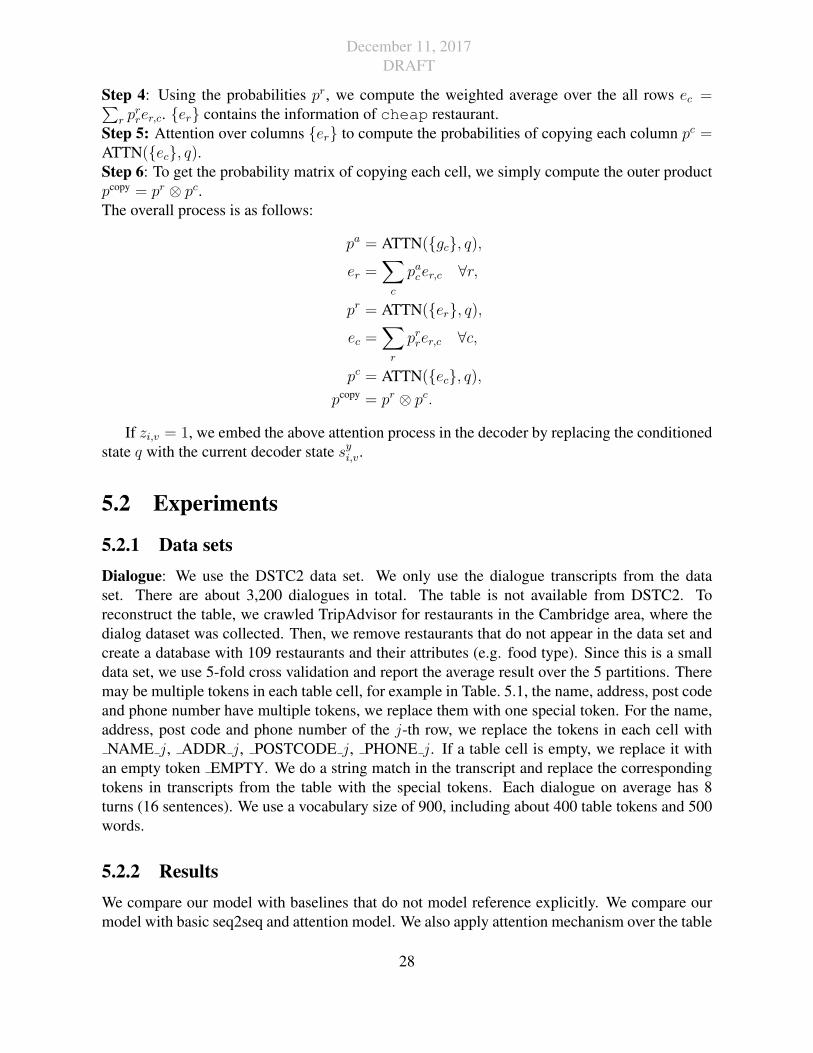
Step 5: Attention over columns {er} to compute the probabilities of copying each column pc =ATTN({ec}, q).Step 6: To get the probability matrix of copying each cell, we simply compute the outer productpcopy = pr ⊗ pc.The overall process is as follows:

pa = ATTN({gc}, q),

er =∑c

pacer,c ∀r,

pr = ATTN({er}, q),

ec =∑r

prrer,c ∀c,

pc = ATTN({ec}, q),pcopy = pr ⊗ pc.

If zi,v = 1, we embed the above attention process in the decoder by replacing the conditionedstate q with the current decoder state syi,v.

5.2 Experiments

5.2.1 Data setsDialogue: We use the DSTC2 data set. We only use the dialogue transcripts from the dataset. There are about 3,200 dialogues in total. The table is not available from DSTC2. Toreconstruct the table, we crawled TripAdvisor for restaurants in the Cambridge area, where thedialog dataset was collected. Then, we remove restaurants that do not appear in the data set andcreate a database with 109 restaurants and their attributes (e.g. food type). Since this is a smalldata set, we use 5-fold cross validation and report the average result over the 5 partitions. Theremay be multiple tokens in each table cell, for example in Table. 5.1, the name, address, post codeand phone number have multiple tokens, we replace them with one special token. For the name,address, post code and phone number of the j-th row, we replace the tokens in each cell withNAME j, ADDR j, POSTCODE j, PHONE j. If a table cell is empty, we replace it with

an empty token EMPTY. We do a string match in the transcript and replace the correspondingtokens in transcripts from the table with the special tokens. Each dialogue on average has 8turns (16 sentences). We use a vocabulary size of 900, including about 400 table tokens and 500words.

5.2.2 ResultsWe compare our model with baselines that do not model reference explicitly. We compare ourmodel with basic seq2seq and attention model. We also apply attention mechanism over the table

28


for dialogue modeling as a baseline. We train all models with simple stochastic gradient descentwith gradient clipping. We use a one-layer LSTM for all RNN components. Hyper-parametersare selected using grid search based on the validation set.

The results for dialogue are shown in Table 5.3. The findings for dialogue are shown in Ta-ble 5.3. Conditioning table performs better in predicting table tokens in general. Table Pointerhas the lowest perplexity for tokens in the table. Since the table tokens appear rarely in the dia-logue transcripts, the overall perplexity does not differ much and the non-table token perplexityare similar. With attention mechanism over the table, the perplexity of table token improves overbasic Seq2Seq model, but still not as good as directly pointing to cells in the table, which showsthe advantage of modeling reference explicitly. As expected, using sentence attention improvessignificantly over models without sentence attention. Surprisingly, Table Latent performs muchworse than Table Pointer. We also measure the perplexity of table tokens that appear only in testset. For models other than Table Pointer, because the tokens never appear in the training set, theperplexity is quite high, while Table Pointer can predict these tokens much more accurately. Thisverifies our conjecture that our model can learn reasoning over databases.

Model All Table Table OOV Word

Seq2Seq 1.35±0.01 4.98±0.38 1.99E7±7.75E6 1.23±0.01Table Attn 1.37±0.01 5.09±0.64 7.91E7±1.39E8 1.24±0.01Table Pointer 1.33±0.01 3.99±0.36 1360 ± 2600 1.23±0.01Table Latent 1.36±0.01 4.99±0.20 3.78E7±6.08E7 1.24±0.01

+ Sentence AttnSeq2Seq 1.28±0.01 3.31±0.21 2.83E9 ± 4.69E9 1.19±0.01Table Attn 1.28±0.01 3.17±0.21 1.67E7±9.5E6 1.20±0.01Table Pointer 1.27±0.01 2.99±0.19 82.86±110 1.20±0.01Table Latent 1.28±0.01 3.26±0.25 1.27E7±1.41E7 1.20±0.01

Table 5.3: Dialogue perplexity results. Table means tokens from table, Table OOV denotes tabletokens that do not appear in the training set. Sentence Attn denotes we use attention mechanismover tokens in utterances from the previous turn.

29


Part III

Structural Bias for Unsupervised Learning

30


Chapter 6

Variational Autoencoders for TextModeling

6.1 Background on Variational Autoencoders

Neural language models [29] typically generate each token xt conditioned on the entire historyof previously generated tokens:

p(x) =∏t

p(xt|x1, x2, ..., xt−1). (6.1)

State-of-the-art language models often parametrize these conditional probabilities using RNNs,which compute an evolving hidden state over the text which is used to predict each xt. Thisapproach, though effective in modeling text, does not explicitly model variance in higher-levelproperties of entire utterances (e.g. topic or style) and thus can have difficulty with heterogeneousdatasets.

Bowman et al. [4] propose a different approach to generative text modeling inspired by relatedwork on vision [20]. Instead of directly modeling the joint probability p(x) as in Equation 6.1,we specify a generative process for which p(x) is a marginal distribution. Specifically, we firstgenerate a continuous latent vector representation z from a multivariate Gaussian prior pθ(z), andthen generate the text sequence x from a conditional distribution pθ(x|z) parameterized using aneural net (often called the generation model or decoder). Because this model incorporates alatent variable that modulates the entire generation of each whole utterance, it may be better ableto capture high-level sources of variation in the data. Specifically, in contrast with Equation 6.1,this generating distribution conditions on latent vector representation z:

pθ(x|z) =∏t

pθ(xt|x1, x2, ..., xt−1, z). (6.2)

To estimate model parameters θ we would ideally like to maximize the marginal probabilitypθ(x) =

∫pθ(z)pθ(x|z)dz. However, computing this marginal is intractable for many decoder

31


choices. Thus, the following variational lower bound is often used as an objective [20]:

log pθ(x) = − log

∫pθ(z)pθ(x|z)dz

≥ Eqφ(z|x)[log pθ(x|z)]− KL(qφ(z|x)||pθ(z)).

Here, qφ(z|x) is an approximation to the true posterior (often called the recognition model orencoder) and is parameterized by φ. Like the decoder, we have a choice of neural architecture toparameterize the encoder. However, unlike the decoder, the choice of encoder does not changethe model class – it only changes the variational approximation used in training, which is afunction of both the model parameters θ and the approximation parameters φ. Training seeks tooptimize these parameters jointly using stochastic gradient ascent. A final wrinkle of the trainingprocedure involves a stochastic approximation to the gradients of the variational objective (whichis itself intractable). We omit details here, noting only that the final distribution of the posteriorapproximation qφ(z|x) is typically assumed to be Gaussian so that a re-parametrization trick canbe used, and refer readers to [20].

6.2 Training Collapse with Textual VAEs

Together, this combination of generative model and variational inference procedure are often re-ferred to as a variational autoencoder (VAE). We can also view the VAE as a regularized versionof the autoencoder. Note, however, that while VAEs are valid probabilistic models whose likeli-hood can be evaluated on held-out data, autoencoders are not valid models. If only the first termof the VAE variational bound Eqφ(z|x)[log pθ(x|z)] is used as an objective, the variance of theposterior probability qφ(z|x) will become small and the training procedure reduces to an autoen-coder. It is the KL-divergence term, KL(qφ(z|x)||pθ(z)), that discourages the VAE memorizingeach x as a single latent point.

While the KL term is critical for training VAEs, historically, instability on text has beenevidenced by the KL term becoming vanishingly small during training, as observed by Bowmanet al. [4]. When the training procedure collapses in this way, the result is an encoder that hasduplicated the Gaussian prior (instead of a more interesting posterior), a decoder that completelyignores the latent variable z, and a learned model that reduces to a simpler language model.We hypothesize that this collapse condition is related to the contextual capacity of the decoderarchitecture. The choice encoder and decoder depends on the type of data. For images, these aretypically MLPs or CNNs. LSTMs have been used for text, but have resulted in training collapseas discussed above [4]. Here, we propose to use a dilated CNN as the decoder instead. In oneextreme, when the effective contextual width of a CNN is very large, it resembles the behaviorof LSTM. When the width is very small, it behaves like a bag-of-words model. The architecturalflexibility of dilated CNNs allows us to change the contextual capacity and conduct experimentsto validate our hypothesis: decoder contextual capacity and effective use of encoding informationare directly related. We next describe the details of our decoder.

32


LSTM zLSTM LSTM

tastes really great

LSTMencoder

CNNDecoder

tastes really great

(a) VAE training graph using a dilated CNN decoder.

BOS

EOStastes really great

tastes really great

inputembedding

dilation=1

dilation=2

z

(b) Digram of dilated CNN decoder.

Figure 6.1: Our training and model architectures for textual VAE using a dilated CNN decoder.

6.3 Dilated Convolutional Decoders

The typical approach to using CNNs used for text generation [17] is similar to that used forimages [13, 22], but with the convolution applied in one dimension. We take this approach herein defining our decoder.

One dimensional convolution: For a CNN to serve as a decoder for text, generation of xtmust only condition on past tokens x<t. Applying the traditional convolution will break thisassumption and use tokens x≥t as inputs to predict xt. In our decoder, we avoid this by simplyshifting the input by several slots [43]. With a convolution with filter size of k and using nlayers, our effective filter size (the number of past tokens to condition to in predicting xt) wouldbe (k − 1)× n+ 1. Hence, the filter size would grow linearly with the depth of the network.

Dilation: Dilated convolution [53] was introduced to greatly increase the effective receptive fieldsize without increasing the computational cost. With dilation d, the convolution is applied so thatd−1 inputs are skipped each step. Causal convolution can be seen a special case with d = 1. Withdilation, the effective receptive size grows exponentially with network depth. In Figure 6.1b, weshow dilation of sizes of 1 and 2 in the first and second layer, respectively. Suppose the dilationsize in the i-th layer is di and we use the same filter size k in all layers, then the effective filtersize is (k − 1)

∑i di + 1. The dilations are typically set to double every layer di+1 = 2di, so the

effective receptive field size can grow exponentially. Hence, the contextual capacity of a CNNcan be controlled across a greater range by manipulating the filter size, dilation size and networkdepth. We use this approach in experiments.

33


ReLU 1x1, 512

ReLU 1xk, 512

conv

ReLU 1x1, 1024

+

conv

conv

Residual connection: We use residual connection [13] in the decoder to speed up conver-gence and enable training of deeper models. We use a residual block (shown to the right) similarto that of [17]. We use three convolutional layers with filter size 1× 1, 1× k, 1× 1, respectively,and ReLU activation between convolutional layers.

Overall architecture: Our VAE architecture is shown in Figure 6.1a. We use LSTM as theencoder to get the posterior probability q(z|x), which we assume to be diagonal Gaussian. Weparametrize the mean µ and variance σ with LSTM output. We sample z from q(z|x), the de-coder is conditioned on the sample by concatenating z with every word embedding of the decoderinput.

6.4 Experiments

6.4.1 Data sets

We use two large scale document classification data sets: Yahoo Answer and Yelp15 review,representing topic classification and sentiment classification data sets respectively [42, 50, 54].The original data sets contain millions of samples, of which we sample 100k as training and10k as validation and test from the respective partitions. The detailed statistics of both data setsare in Table 6.1. Yahoo Answer contains 10 topics including Society & Culture, Science &Mathematics etc. Yelp15 contains 5 level of rating, with higher rating better.

Data classes documents average #w vocabulary

Yahoo 10 100k 78 200kYelp15 5 100k 96 90k

Table 6.1: Data statistics

34


6.4.2 ResultsWe use an LSTM as an encoder for VAE and explore LSTMs and CNNs as decoders. ForCNNs, we explore several different configurations. We set the convolution filter size to be 3 andgradually increase the depth and dilation from [1, 2, 4], [1, 2, 4, 8, 16] to [1, 2, 4, 8, 16, 1, 2, 4,8, 16]. They represent small, medium and large model and we name them as SCNN, MCNN andLCNN. We also explore a very large model with dilations [1, 2, 4, 8, 16, 1, 2, 4, 8, 16, 1, 2, 4,8, 16] and name it as VLCNN. The effective filter size are 15, 63, 125 and 187 respectively. Weuse the last hidden state of the encoder LSTM and feed it though an MLP to get the mean andvariance of q(z|x), from which we sample z and then feed it through an MLP to get the startingstate of decoder. For the LSTM decoder, we follow [4] to use it as the initial state of LSTM andfeed it to every step of LSTM. For the CNN decoder, we concatenate it with the word embeddingof every decoder input.

The results for language modeling are shown in Table 6.2. We report the negative log like-lihood (NLL) and perplexity (PPL) of the test set. For the NLL of VAEs, we decompose it intoreconstruction loss and KL divergence and report the KL divergence in the parenthesis.

We first look at the LM results for Yahoo data set. As we gradually increase the effective filtersize of CNN from SCNN, MCNN to LCNN, the NLL decreases from 345.3, 338.3 to 335.4. TheNLL of LCNN-LM is very close to the NLL of LSTM-LM 334.9. But VLCNN-LM is a little bitworse than LCNN-LM, this indicates a little bit of over-fitting.

We can see that LSTM-VAE is worse than LSTM-LM in terms of NLL and the KL term isnearly zero, which verifies the finding of [4]. When we use CNNs as the decoders for VAEs, wecan see improvement over pure CNN LMs. For SCNN, MCNN and LCNN, the VAE results im-prove over LM results from 345.3 to 337.8, 338.3 to 336.2, and 335.4 to 333.9 respectively. Theimprovement is big for small models and gradually decreases as we increase the decoder modelcontextual capacity. When the model is as large as VLCNN, the improvement diminishes and theVAE result is almost the same with LM result. This is also reflected in the KL term, SCNN-VAEhas the largest KL of 13.3 and VLCNN-VAE has the smallest KL of 0.7. When LCNN is usedas the decoder, we obtain an optimal trade off between using contextual information and latentrepresentation. LCNN-VAE achieves a NLL of 333.9, which improves over LSTM-LM withNLL of 334.9.

We find that if we initialize the parameters of LSTM encoder with parameters of LSTMlanguage model, we can improve the VAE results further. This indicates better encoder modelis also a key factor for VAEs to work well. Combined with encoder initialization, LCNN-VAEimproves over LSTM-LM from 334.9 to 332.1 in NLL and from 66.2 to 63.9 in PPL. Similarresults for the sentiment data set are shown in Table 6.2b. LCNN-VAE improves over LSTM-LMfrom 362.7 to 359.1 in NLL and from 42.6 to 41.1 in PPL.

35


Model Size NLL (KL) PPL

LSTM-LM < i 334.9 66.2LSTM-VAE∗∗ < i 342.1 (0.0) 72.5LSTM-VAE∗∗ + init < i 339.2 (0.0) 69.9

SCNN-LM 15 345.3 75.5SCNN-VAE 15 337.8 (13.3) 68.7SCNN-VAE + init 15 335.9 (13.9) 67.0

MCNN-LM 63 338.3 69.1MCNN-VAE 63 336.2 (11.8) 67.3MCNN-VAE + init 63 334.6 (12.6) 66.0

LCNN-LM 125 335.4 66.6LCNN-VAE 125 333.9 (6.7) 65.4LCNN-VAE + init 125 332.1 (10.0) 63.9

VLCNN-LM 187 336.5 67.6VLCNN-VAE 187 336.5 (0.7) 67.6VLCNN-VAE + init 187 335.8 (3.8) 67.0

(a) Yahoo

Model Size NLL (KL) PPL

LSTM-LM < i 362.7 42.6LSTM-VAE∗∗ < i 372.2 (0.3) 47.0LSTM-VAE∗∗ + init < i 368.9 (4.7) 46.4

SCNN-LM 15 371.2 46.6SCNN-VAE 15 365.6 (9.4) 43.9SCNN-VAE + init 15 363.7 (10.3) 43.1

MCNN-LM 63 366.5 44.3MCNN-VAE 63 363.0 (6.9) 42.8MCNN-VAE + init 63 360.7 (9.1) 41.8

LCNN-LM 125 363.5 43.0LCNN-VAE 125 361.9 (6.4) 42.3LCNN-VAE + init 125 359.1 (7.6) 41.1

VLCNN-LM 187 364.8 43.7VLCNN-VAE 187 364.3 (2.7) 43.4VLCNN-VAE + init 187 364.7 (2.2) 43.5

(b) Yelp

Table 6.2: Language modeling results on the test set. ∗∗ is from [4]. We report negative loglikelihood (NLL) and perplexity (PPL) on the test set. The KL component of NLL is given inparentheses. Size indicates the effective filter size. VAE + init indicates pretraining of only theencoder using an LSTM LM.

36


Chapter 7

Proposed work

7.1 Unsupervised Natural Language LearningTo continue the line of work of unsupervised learning, I would like to investigate the naturallanguage generation problem. Previously natural language generation mainly relies on languagemodels. Recurrent neural networks (RNNs) have achieved the state of the art in language model-ing. However, RNN alone lacks the ability to generate languages with desired attributes. Gener-ating sentences with desired attributes are useful for many applications. For example, in reviewgenerations, we would like to condition the generation on the ratings. For dialogue modeling,the response is generated conditioning on given intents.

Variational auto-encoders are potential solutions to generate sentences with desired attributes.But there are some inherent limitations with variational autoencoders for text modeling, as men-tioned in Chapter 6. [15] is a preliminary work in this direction. It combines language modelingwith generative adversarial network [12]. The generated sentences are fed to a discriminator andwe can directly use backpropagation to ensure that sentences have certain attributes. Based onthe success, we would like to investigate style transfer for text, dialogue modeling with intentetc.

7.2 Timeline• Now - April 2018: work on natural language generation.• April 2018 - May 2018: wrap up work into a final thesis.• June 2018: thesis defense.

37


Bibliography

[1] Stanislaw Antol, Aishwarya Agrawal, Jiasen Lu, Margaret Mitchell, Dhruv Batra,C Lawrence Zitnick, and Devi Parikh. Vqa: Visual question answering. arXiv preprintarXiv:1505.00468, 2015. 4.2.1, 4.2.2, ??

[2] Dzmitry Bahdanau, Kyunghyun Cho, and Yoshua Bengio. Neural machine translationby jointly learning to align and translate. CoRR, abs/1409.0473, 2014. URL http://arxiv.org/abs/1409.0473. 5.1

[3] Dzmitry Bahdanau, Kyunghyun Cho, and Yoshua Bengio. Neural machine translation byjointly learning to align and translate. arXiv preprint arXiv:1409.0473, 2014. 4

[4] Samuel R Bowman, Luke Vilnis, Oriol Vinyals, Andrew M Dai, Rafal Jozefowicz,and Samy Bengio. Generating sentences from a continuous space. arXiv preprintarXiv:1511.06349, 2015. 6.1, 6.2, 6.4.2, 6.2

[5] Wenlin Chen, James T. Wilson, Stephen Tyree, Kilian Q. Weinberger, and Yixin Chen.Compressing neural networks with the hashing trick. 2015. 3.3.2

[6] Maxwell D. Collins and Pushmeet Kohli. Memory bounded deep convolutional networks.Technical report, University of Wisconsin-Madison, 2014. 3.3.2

[7] B. Dai, B. Xie, N. He, Y. Liang, A. Raj, M. Balcan, and L. Song. Scalable kernel methodsvia doubly stochastic gradients. 2014. ??, 3.1, 3.3.1

[8] Misha Denil, Babak Shakibi, Laurent Dinh, Marc’Aurelio Ranzato, and Nando de Freitas.Predicting parameters in deep learning. pages 2148–2156, 2013. 3.2, 3.3.2

[9] A. Doucet, N. de Freitas, and N. Gordon. Sequential Monte Carlo Methods in Practice.Springer-Verlag, 2001. 2.2.2

[10] Hao Fang, Saurabh Gupta, Forrest Iandola, Rupesh Srivastava, Li Deng, Piotr Dollar, Jian-feng Gao, Xiaodong He, Margaret Mitchell, John Platt, et al. From captions to visualconcepts and back. arXiv preprint arXiv:1411.4952, 2014. 4.1.2, 4.2.1

[11] Haoyuan Gao, Junhua Mao, Jie Zhou, Zhiheng Huang, Lei Wang, and Wei Xu. Are youtalking to a machine? dataset and methods for multilingual image question answering.arXiv preprint arXiv:1505.05612, 2015. 4.1.1

[12] Ian Goodfellow, Jean Pouget-Abadie, Mehdi Mirza, Bing Xu, David Warde-Farley, SherjilOzair, Aaron Courville, and Yoshua Bengio. Generative adversarial nets. In Advances inneural information processing systems, pages 2672–2680, 2014. 7.1

[13] Kaiming He, Xiangyu Zhang, Shaoqing Ren, and Jian Sun. Deep residual learning for

38

http://arxiv.org/abs/1409.0473

http://arxiv.org/abs/1409.0473


image recognition. In Proceedings of the IEEE Conference on Computer Vision and PatternRecognition, pages 770–778, 2016. 6.3, 6.3

[14] Matthew Henderson, Blaise Thomson, and Jason Williams. Dialog state tracking challenge2 & 3, 2014. 5.1

[15] Zhiting Hu, Zichao Yang, Xiaodan Liang, Ruslan Salakhutdinov, and Eric P Xing. Con-trollable text generation. arXiv preprint arXiv:1703.00955, 2017. 7.1

[16] Yangqing Jia, Evan Shelhamer, Jeff Donahue, Sergey Karayev, Jonathan Long, Ross Gir-shick, Sergio Guadarrama, and Trevor Darrell. Caffe: Convolutional architecture for fastfeature embedding. ArXiv, 1408.5093, 2014. 3.3

[17] Nal Kalchbrenner, Lasse Espeholt, Karen Simonyan, Aaron van den Oord, Alex Graves,and Koray Kavukcuoglu. Neural machine translation in linear time. arXiv preprintarXiv:1610.10099, 2016. 6.3, 6.3

[18] Yoon Kim. Convolutional neural networks for sentence classification. arXiv preprintarXiv:1408.5882, 2014. 4.1.2

[19] G. S. Kimeldorf and G. Wahba. A correspondence between Bayesian estimation on stochas-tic processes and smoothing by splines. Annals of Mathematical Statistics, 41:495–502,1970. 2.1.1

[20] Diederik P Kingma and Max Welling. Auto-encoding variational bayes. arXiv preprintarXiv:1312.6114, 2013. 6.1, 6.1

[21] Alex Krizhevsky, Ilya Sutskever, and Geoffrey E. Hinton. Imagenet classification with deepconvolutional neural networks. pages 1106–1114, 2012. 1, 3.3

[22] Alex Krizhevsky, Ilya Sutskever, and Geoffrey E Hinton. Imagenet classification with deepconvolutional neural networks. In Advances in neural information processing systems,pages 1097–1105, 2012. 4.1.1, 6.3

[23] Q.V. Le, T. Sarlos, and A. J. Smola. Fastfood — computing hilbert space expansions inloglinear time. In International Conference on Machine Learning, 2013. 2.1.2, 2.2.2

[24] Tsung-Yi Lin, Michael Maire, Serge Belongie, James Hays, Pietro Perona, Deva Ramanan,Piotr Dollar, and C Lawrence Zitnick. Microsoft coco: Common objects in context. InComputer Vision–ECCV 2014, pages 740–755. Springer, 2014. 4.2.1

[25] Lin Ma, Zhengdong Lu, and Hang Li. Learning to answer questions from image usingconvolutional neural network. arXiv preprint arXiv:1506.00333, 2015. 4.1.1, 4.2.2

[26] Mateusz Malinowski and Mario Fritz. A multi-world approach to question answering aboutreal-world scenes based on uncertain input. In Advances in Neural Information ProcessingSystems, pages 1682–1690, 2014. 4.2.2

[27] Mateusz Malinowski, Marcus Rohrbach, and Mario Fritz. Ask your neurons: A neural-based approach to answering questions about images. arXiv preprint arXiv:1505.01121,2015. 4.2.2

[28] J. Mercer. Functions of positive and negative type and their connection with the theoryof integral equations. Philos. Trans. R. Soc. Lond. Ser. A Math. Phys. Eng. Sci., A 209:

39


415–446, 1909. 2.1.1, 2.1.1

[29] Tomas Mikolov, Martin Karafiat, Lukas Burget, Jan Cernocky, and Sanjeev Khudanpur.Recurrent neural network based language model. In Interspeech, volume 2, page 3, 2010.6.1

[30] Radford M. Neal. Assessing relevance determination methods using delve. In C. M. Bishop,editor, Neural Networks and Machine Learning, pages 97–129. Springer, 1998. 2.2.3, 2.3

[31] A. Rahimi and B. Recht. Weighted sums of random kitchen sinks: Replacing minimizationwith randomization in learning. 2009. 2.1.2, 2.1.2

[32] Mengye Ren, Ryan Kiros, and Richard Zemel. Exploring models and data for image ques-tion answering. arXiv preprint arXiv:1505.02074, 2015. 4.1.1, 4.2.2

[33] Tara N. Sainath, Brian Kingsbury, Vikas Sindhwani, Ebru Arisoy, and Bhuvana Ramabhad-ran. Low-rank matrix factorization for deep neural network training with high-dimensionaloutput targets. pages 6655–6659, 2013. 3.2, 3.3.2

[34] I. Schoenberg. Positive definite functions on spheres. Duke Math. J., 9:96–108, 1942. 2.1.2

[35] B. Scholkopf, R. Herbrich, and A. J. Smola. A generalized representer theorem. In D. P.Helmbold and B. Williamson, editors, Proc. Annual Conf. Computational Learning The-ory, number 2111 in Lecture Notes in Comput. Sci., pages 416–426, London, UK, 2001.Springer-Verlag. 2.1.1

[36] Iulian V Serban, Alessandro Sordoni, Yoshua Bengio, Aaron Courville, and Joelle Pineau.Building end-to-end dialogue systems using generative hierarchical neural network models.In Proceedings of the 30th AAAI Conference on Artificial Intelligence (AAAI-16), 2016. 5.1

[37] Yelong Shen, Xiaodong He, Jianfeng Gao, Li Deng, and Gregoire Mesnil. A latent semanticmodel with convolutional-pooling structure for information retrieval. In Proceedings ofthe 23rd ACM International Conference on Conference on Information and KnowledgeManagement, pages 101–110. ACM, 2014. 4.1.2

[38] B. W. Silverman. Density Estimation for Statistical and Data Analysis. Monographs onstatistics and applied probability. Chapman and Hall, London, 1986. 2.2.1

[39] Karen Simonyan and Andrew Zisserman. Very deep convolutional networks for large-scaleimage recognition. arXiv preprint arXiv:1409.1556, 2014. 4.1.1

[40] Ilya Sutskever, Oriol Vinyals, and Quoc VV Le. Sequence to sequence learning with neuralnetworks. In Advances in neural information processing systems, pages 3104–3112, 2014.1, 4.1.2

[41] Christian Szegedy, Wei Liu, Yangqing Jia, Pierre Sermanet, Scott Reed, DragomirAnguelov, Dumitru Erhan, Vincent Vanhoucke, and Andrew Rabinovich. Going deeperwith convolutions. arXiv preprint arXiv:1409.4842, 2014. 4.1.1

[42] Duyu Tang, Bing Qin, and Ting Liu. Document modeling with gated recurrent neuralnetwork for sentiment classification. In EMNLP, pages 1422–1432, 2015. 6.4.1

[43] Aaron van den Oord, Nal Kalchbrenner, Lasse Espeholt, Oriol Vinyals, Alex Graves, et al.Conditional image generation with pixelcnn decoders. In Advances in Neural Information

40


Processing Systems, pages 4790–4798, 2016. 6.3

[44] A. G. Wilson and R. P. Adams. Gaussian process kernels for pattern discovery and extrap-olation. In Proceedings of the 30th International Conference on Machine Learning, 2013.2.2.1

[45] Kelvin Xu, Jimmy Ba, Ryan Kiros, Aaron Courville, Ruslan Salakhutdinov, Richard Zemel,and Yoshua Bengio. Show, attend and tell: Neural image caption generation with visualattention. arXiv preprint arXiv:1502.03044, 2015. 4

[46] Zichao Yang, Marcin Moczulski, Misha Denil, Nando de Freitas, Alex Smola, Le Song, andZiyu Wang. Deep fried convnets. In Proceedings of the IEEE International Conference onComputer Vision, pages 1476–1483, 2015. 1

[47] Zichao Yang, Andrew Wilson, Alex Smola, and Le Song. A la carte–learning fast kernels.In Artificial Intelligence and Statistics, pages 1098–1106, 2015. 1

[48] Zichao Yang, Phil Blunsom, Chris Dyer, and Wang Ling. Reference-aware language mod-els. arXiv preprint arXiv:1611.01628, 2016. 1

[49] Zichao Yang, Xiaodong He, Jianfeng Gao, Li Deng, and Alex Smola. Stacked attention net-works for image question answering. In Proceedings of the IEEE Conference on ComputerVision and Pattern Recognition, pages 21–29, 2016. 1

[50] Zichao Yang, Diyi Yang, Chris Dyer, Xiaodong He, Alex Smola, and Eduard Hovy. Hi-erarchical attention networks for document classification. In Proceedings of NAACL-HLT,pages 1480–1489, 2016. 6.4.1

[51] Zichao Yang, Zhiting Hu, Ruslan Salakhutdinov, and Taylor Berg-Kirkpatrick. Improvedvariational autoencoders for text modeling using dilated convolutions. arXiv preprintarXiv:1702.08139, 2017. 1

[52] Jason Yosinski, Jeff Clune, Yoshua Bengio, and Hod Lipson. How transferable are featuresin deep neural networks? pages 3320–3328. 2014. 3.3.1

[53] Fisher Yu and Vladlen Koltun. Multi-scale context aggregation by dilated convolutions.arXiv preprint arXiv:1511.07122, 2015. 6.3

[54] Xiang Zhang, Junbo Zhao, and Yann LeCun. Character-level convolutional networks fortext classification. arXiv preprint arXiv:1509.01626, 2015. 6.4.1

41

thesis proposal - carnegie mellon school of …zichaoy/proposal.pdf · december 11, 2017 draft ules...

Documents