Relative Distance Measurement using GPS and Internal Vehicle Sensors

Master of Science Thesis in the Master’s Programme Communication Engineering

AHMET IRKIN SERKAN KARAKIS Department of Signals and Systems Division of Signal Processing and Biomedical Engineering CHALMERS UNIVERSITY OF TECHNOLOGY Göteborg, Sweden 2011 Master’s Thesis 2011:15

MASTER’S THESIS 2011:15

Relative Distance Measurement

using GPS and Internal Vehicle Sensors

Master of Science Thesis in the Master’s Programme Communication Engineering

AHMET IRKIN

SERKAN KARAKIS

Department of Signals and Systems Division of Signal Processing and Biomedical Engineering

CHALMERS UNIVERSITY OF TECHNOLOGY

Göteborg, Sweden 2011

Relative Distance Measurement using GPS and Internal Vehicle Sensors Master of Science Thesis in the Master’s Programme Communication Engineering

AHMET IRKIN

SERKAN KARAKIS

© AHMET IRKIN, SERKAN KARAKIS, 2011

Examensarbete / Institutionen för Signaler och System, Chalmers tekniska högskola, 2011:15

Department of Signals and Systems

Division of Signal Processing and Biomedical Engineering

Chalmers University of Technology

SE‐412 96 Göteborg

Sweden

Telephone: + 46 (0)31‐772 1000

Cover: A visual of the Vehicle‐to‐Vehicle communications, of which this thesis work presents one of the benefits: relative positioning of target vehicles.

Department of Signals and Systems Göteborg, Sweden 2011

Kommentar [mp1]: If the report is printed by for instance Chalmers reproservice, this name should be inserted here. If else the department name should be given.

i

Relative Distance Measurement using GPS and Internal Vehicle Sensors

Master of Science Thesis in the Master’s Programme Communication Engineering

AHMET IRKIN

SERKAN KARAKIS Department of Signals and Systems Division of Signal Processing and Biomedical Engineering Chalmers University of Technology

ABSTRACT

Each year a million people are being injured in traffic accidents. New active safety systems

have recently been introduced on the market that may significantly reduce the effect of collisions

and sometimes even avoid them (Ref City Safety). In order to prevent an accident there is a need to

first assess and understand the traffic situation around the vehicle. The current state of the art

active safety systems utilize radars, cameras and laser based sensors to support environmental

sensing, i.e., to position the neighboring vehicles in relation to the host vehicle and the

infrastructure (roads, intersections, etc.). Future safety systems will obtain additional information by

communicating with other vehicles and the infrastructure, also by including new sensors like a GPS

and a map. Such information may dramatically improve the accuracy of our understanding the traffic

situation, but as of now, the design of such systems has not been studied much.

This master thesis investigates how to combine information from several sensors including

GPS and internal vehicle sensors in order to position the ego vehicle and other objects around the

vehicle. Apart from designing the positioning systems, we also wish to identify difficulties and

understand different parts of the problem. These parts include sensor models, sensor fusion

algorithms and techniques to handle data that arrives with a time delay.

ii

ACKNOWLEDGMENTS

We would like to thank our examiner Lennart Svensson from Chalmers and our supervisor

Henrik Lind from Volvo Car Corporation so much for bringing this interesting thesis work to us and

also for their continuous support throughout our work.

We also thank Volvo Car Corporation and especially Mats Lestander for making the thesis

work possible with providing everything we needed during the project.

iii

TABLE OF CONTENTS

Abstract ......................................................................................................................................... i

Acknowledgments ........................................................................................................................ ii

Table of Contents ........................................................................................................................ iii

List of Abbreviations ..................................................................................................................... v

Table of Figures ........................................................................................................................... vi

1 Introduction ........................................................................................................................ 1

1.1 Thesis Background .......................................................................................................... 1

1.2 Aim of the Thesis ............................................................................................................. 2

1.3 Methodology ................................................................................................................... 2

1.4 Description of Test Equipment and Configurations ........................................................ 2

1.5 Limitations ....................................................................................................................... 4

1.6 Outline of the Report ...................................................................................................... 5

2 Technical Overview ............................................................................................................. 6

2.1 Principles of GPS ............................................................................................................. 6

2.1.1 GPS Signal ................................................................................................................ 6

2.1.2 Determining Receiver Position ................................................................................ 7

2.1.3 GPS Messages ......................................................................................................... 8

2.1.4 GPS Data Error ...................................................................................................... 12

2.2 Coordinate Systems ...................................................................................................... 12

2.2.1 Geographical Coordinate System .......................................................................... 13

2.2.2 Earth‐Centered Earth‐Fixed Coordinate System ................................................... 13

2.2.3 Map Projection ...................................................................................................... 14

2.2.4 Elliptic Parameters of the Earth for GPS Applications .......................................... 15

iv

2.3 Internal Vehicle Sensors ................................................................................................ 16

2.4 Sensor Fusion Systems .................................................................................................. 17

2.4.1 Inertial Navigation System .................................................................................... 18

2.4.2 Kalman Filter ......................................................................................................... 18

3 Mathematical Model of Algorithms and Configuration .................................................... 21

3.1 Overview of the Algorithm ............................................................................................ 21

3.1.1 Synchronization of GPS and Internal Sensors ....................................................... 22

3.1.2 Parameters of the Kalman Filter ........................................................................... 23

3.1.3 Detection of Signal Qualities for GPS and Internal Sensors .................................. 27

3.1.4 Relative Distance Measurement ........................................................................... 28

4 Results ............................................................................................................................... 30

4.1 Test case – 1 .................................................................................................................. 30

4.2 Test case – 2 .................................................................................................................. 34

5 Conclusion and Future Work ............................................................................................ 43

Bibliography ................................................................................................................................ 44

v

LIST OF ABBREVIATIONS

CAN Controller Area Network

ECEF Earth‐Centered Earth‐Fixed

GPS Global Positioning System

HS‐CAN High Speed ‐ Controller Area Network

Hz Hertz

IEEE Institute of Electrical and Electronics Engineers

INS Inertial Navigation System

ITS Intelligent Transportation Systems

LPF Low‐Pass‐Filter

NGA National Geospatial – Intelligence Agency

NIMA National Imagery and Mapping Agency

NMEA National Marine Electronics Association

SNR Signal to Noise Ratio

V2V Vehicle to Vehicle

WAVE Wireless Access for Vehicular Environments

WGS World Geodetic System

WLAN Wireless Local Area Network

latitude

longitude

h altitude

vi

TABLE OF FIGURES

Figure 1.1 ‐ Overview of device connections .......................................................................................... 3

Figure 2.1 ‐ Calculation of satellite distance ........................................................................................... 7

Figure 2.2 ‐ Visualization of GPS positioning .......................................................................................... 8

Figure 2.3 ‐ ECEF and Geodetic coordinates ......................................................................................... 14

Figure 2.4 ‐ Mercator projection ........................................................................................................... 15

Figure 2.5 ‐ Low pass filter applied to yaw rate .................................................................................... 17

Figure 2.6 ‐ Visualization of the Kalman gain ........................................................................................ 19

Figure 3.1 ‐ Overview of the sensor fusion system ............................................................................... 22

Figure 3.2 ‐ The Kalman filter algorithm ............................................................................................... 25

Figure 3.3 ‐ Relative distance measurement ........................................................................................ 29

Figure 4.1 ‐ Test track 1 ......................................................................................................................... 30

Figure 4.2 ‐ Vehicle speed ..................................................................................................................... 31

Figure 4.3 ‐ Lateral distance .................................................................................................................. 31

Figure 4.4 ‐ Longitudinal distance ......................................................................................................... 32

Figure 4.5 ‐ Target angle ....................................................................................................................... 32

Figure 4.6 ‐ Lateral error histogram ...................................................................................................... 33

Figure 4.7 ‐ Longitudinal error histogram ............................................................................................. 33

Figure 4.8 ‐ Target angle error histogram ............................................................................................. 34

Figure 4.9 ‐ Test track 2 ......................................................................................................................... 35

Figure 4.10 ‐ Vehicle speed ................................................................................................................... 36

Figure 4.11 ‐ Lateral distance ................................................................................................................ 36

Figure 4.12 ‐ Longitudinal distance ....................................................................................................... 37

Figure 4.13 ‐ Target angle ..................................................................................................................... 37

Figure 4.14 ‐ Absolute distance error ................................................................................................... 38

Figure 4.15 ‐ Lateral error histogram .................................................................................................... 38

Figure 4.16 ‐ Longitudinal error histogram ........................................................................................... 39

Figure 4.17 ‐ Target angle error histogram ........................................................................................... 39

Figure 4.18 ‐ GPS clock error ................................................................................................................. 42

1

INTRODUCTION

In this section, the background of our thesis work will be introduced to the reader and the

goals will be defined. Technical equipments used in the project will also be briefly introduced. In

addition, the assumptions made, and the limitations put in the work will be presented. Finally, an

outline of the report is given at the end of the section.

1.1 Thesis Background

Today’s active safety systems utilize radars, cameras and laser based sensors to support

environmental sensing, i.e., to position the neighboring vehicles in relation to the host vehicle and

the infrastructure (roads, intersections, etc.). Systems capability is dependent on the limits of the

sensors which allow tracking of objects only in view of the sensors. Future safety systems will obtain

additional information by communicating with other vehicles and the infrastructure, also by

including new sensors such as a GPS. Such information may dramatically improve the accuracy of our

understanding the traffic situation and reduce possibility of accidents, but as of now, the design of

such systems has not been studied much.

In this thesis work relative distance calculation to support V2V communication is presented.

Considering the short distance between the cars driving on the road and using similar GPS receiver

products, it is practical to assume that they may have common errors ( ) and also vehicle specific

errors ( ) in their individual position estimations. Therefore, we can define the equation of the

position estimation for each vehicle as follows:

Our expectation was although each vehicle had erroneous position estimation with the model

defined above; differentiation could discard the common error included in both vehicle positions.

To evaluate this idea, we logged and organized the necessary information and implemented a

system to make the best position estimations. In order to reduce the vehicle specific errors in the

calculations, other inputs (yaw rate, speed, gear, etc.) are also introduced to the system and

combined with a sensor fusion algorithm. There are different methods and algorithms such as

Kalman Filtering, Bayesian Networks, Dempster‐Shafer Theory and etc. used to implement a sensor

2

fusion system for different applications. A Kalman filter is used for improving position and thereby

distance measurements in this master thesis work.

1.2 Aim of the Thesis

The target of this thesis work is to investigate the possible improvements in collision

avoidance systems that might become available with V2V communication. The main goals of our

work are determining the relative distance of a target vehicle with respect to the ego vehicle as they

share GPS and internal vehicle sensor information such as speed, yaw rate, steering angle and

analyzing the accuracy, dependencies and challenges of such a system.

As of now, several associations and corporations are working on V2V communication

standards. One of them, IEEE, has recently developed the 802.11p standard, the so‐called Wireless

Access for Vehicular Environments (WAVE) for Intelligent Transportation Systems (ITS), which brings

a set of adjustments to the well‐known 802.11 WLAN protocol [1]. However, during this thesis work,

although the vehicles did not have such built‐in communication system physically, we assumed that

they had one and they could share the necessary information with each other.

1.3 Methodology

To design an accurate and efficient sensor fusion system, the principles of GPS and the vehicle

sensors are studied first. Once the strengths and weaknesses of each of them are grasped, the

necessary sensors are chosen to be inputs to the system. The next thing is to choose the sensor

fusion algorithm and define the equations to combine the inputs in a reasonable way. After the

equations are defined and the sensor fusion algorithm is developed, CANalyzer software to log

information from CAN bus of the vehicle is installed and a C++ code is written to record GPS

information. Small test data is logged to analyze and solve synchronization problem and once all the

information is synchronized, the sensor fusion algorithm is developed in MATLAB. When the

software and the hardware are prepared, test scenarios are created and thereby tests are done

according to them. Finally, results of the tests are analyzed and presented.

1.4 Description of Test Equipment and Configurations

Test vehicles that were used in our project are standard 2007 Volvo S80 sedan and 2008 Volvo

V70 station wagon. Both vehicles are equipped with GlobalSat BU‐353 GPS receiver, standard

internal sensors (speed, yaw, gear) and only S80 had integrated Radar‐Camera sensor.

3

GPS Receiver

GlobalSat BU‐353 GPS receiver was used in this thesis work. GPS receiver is equipped with a

high performance SiRF Star III GPS chipset, which outputs the information in NMEA 0183 format

through its USB interface. We used GPRMC, GPGGA and GPGSV messages of NMEA 0183 output in

our project.

Table 1 ‐ Sampling frequency of GPS data

Source Sampling Time Sampling Frequency

GPRMC GPS 1 sec 1 Hz

Latitude

Longitude

Speed

Time

GPGGA 1 sec 1 Hz

Number of Satellites

GPGSV 5 sec 0.2 Hz

SNR

Controller Area Network (CAN) & Vector CANcaseXL

Controller area network (CAN) is a serial bus communication protocol suited for networking

sensors, actuators and other nodes in real time systems [2]. The protocol is widely used in the

automotive industry. CAN messages are kept in four different formats as data, remote, error and

overload. In our project, data messages are used. CAN message frame consists of Start of Frame

(SOF), Identifier, Remote Transmission Request (RTR), Control, Data, Cyclic Redundancy Checksum

(CRC), Acknowledgement (ACK) and End of Frame (EOF).

Figure 0.1 ‐ Overview of device connections

CANcase XL CANalyzer

GPS Logger

4

SOF Identifier RTR Control Data CRC ACK EOF

Vector CANcaseXL is a USB interface, which is capable of processing CAN messages. It is

possible to receive and analyze remote frames without any limitation. It is also capable of generating

and detecting error frames on the CAN bus [3]. CANcaseXL works with the Vector CANalyzer

software.

Vector CANalyzer is a software tool, which is used for analyzing and observing ECU networks

and distributed systems in vehicles. In this thesis work, we used CANalyzer tool in order to observe,

analyze and record data traffic in CAN.

We logged speed, gear and yaw rate information from High Speed Control Area Network (HS‐

CAN). The sampling frequencies of these signals are shown in the table below.

Table 2 ‐ Sampling frequency of sensor data

Source Sampling Time Sampling Frequency

Speed High Speed CAN 20 ms 50 Hz

Gear 20 ms 50 Hz

Yaw 20 ms 50 Hz

Distance Radar 100 ms 10 Hz

Yaw 20 ms 50 Hz

1.5 Limitations

In principal, the system that is developed in this thesis work relies on accuracy and efficiency

of the communication link between the vehicles. However, since we did not use an actual

communication system, we assumed existence of a link to share the information in between.

Therefore, the outcomes of this thesis work should be seen as the results obtained using a perfect

communication system with high data rate.

Another important assumption is the absolute accuracy of the reference data, with which we

compare our test results. We used the information from the radar enhanced with a camera in order

to obtain the true distance between the vehicles and compared our results with that information.

Consequently, the accuracy of our test results is relative to the accuracy of the radar information.

5

Moreover, since we used the radar‐camera information as the reference and they required a

line of sight view within a narrow angle of the target vehicle for distance determination, we could

only test the cases where the vehicles were following each other or at least they drove in front of

each other.

1.6 Outline of the Report

The report starts with the aim of this thesis work and the theoretical background of the

problem we are dealing with. The hardware and the software equipments used in this job are

introduced and the limitations are given to assist the reader why we have made certain decisions in

the design.

After this brief introduction, a detailed overview of GPS and vehicle sensors including working

principles, technical specifications, strengths and weaknesses is presented. The formal sensor fusion

algorithm and the effects of its parameters are explained.

In the third chapter, an overview of the entire algorithm including inputs of the sensor fusion

system, solution to synchronization problem and vehicle dynamics equations is given.

Results obtained from the tests are shown in the results section; the comments and possible

work for the future are presented in the conclusion.

6

TECHNICAL OVERVIEW

In this section, some important background information is given to help the reader follow the

rest of the report easier. Main areas discussed are principles of the Global Positioning System (GPS),

coordinate systems, internal vehicle sensors and sensor fusion systems, particularly the Kalman

Filter which is used in our project.

1.7 Principles of GPS

Global positioning system (GPS) is a satellite based positioning system. GPS satellites convey

information data, which can be used to calculate the position of the receiver. GPS includes 28 active

satellites that are uniformly settled on six different circular orbits. Inclination angle of orbits from

the equator is 55° and orbits are seperated by 60° right accession from each other[4]. This

constellation provides global coverage and chance to operate 24 hours a day and in all weather

conditions. In theory three or more satellites in view is enough to calculate the location of the

receiver. Although receiver can calculate the position, the accuracy of positioning is dependent on

the number of satellites in view, signal qualities, weather conditions, etc.

1.7.1 GPS Signal

Each GPS satellite conveys navigation message, which is made of five major components [4].

1. Satellite Almanac Data

Satellite Almanac Data includes orbital information for each satellite in the system. The

receiver uses Almanac Data to calculate the approximate location of each satellite at any time.

2. Satellite Ephemeris Data

Satellite Ephemeris Data gives much more accurate information about satellite locations.

Ephemeris data is conveyed from a particular satellite and it only includes location of that satellite,

and it is valid for only several hours [4].

3. Signal Timing Data

GPS data includes time tags, which are used to calculate transmission time of specific points

on the GPS signal. This information is needed to determine the satellite‐to‐user propagation delay

used for ranging[4].

4. Ionospheric Delay Data

7

Ionospheric delay data includes estimated amount of delay, when signal passes through

ionosphere.

5. Satellite Health Message

Satellite health message carries information about satellite operating status.

1.7.2 Determining Receiver Position

Each satellite transmits its exact orbital position and onboard clock time. The signal is

transmitted at speed of light (300 10 / ). Time difference between the transmission of the

signal by the satellite and the received time by the receiver is called transit time. Distance between

the receiver and the satellite is then calculated by multiplying the speed of light and the transit time

( ).

c

Figure 0.1 ‐ Calculation of satellite distance

The distance from a certain satellite provides a range circle, which indicates all the possible

positions of the receiver. Each satellite points a different range circle. In an ideal case, the range

circles are represented with solid line circles shown in Figure 0.2. Intersection of these circles gives

the estimated receiver position. However, these range circles are sensitive to errors and considering

the fact that the signal propagates with speed of light, even small clock errors may cause large

positioning errors. For this reason, the GPS receiver clock and the satellite clock are synchronized to

8

provide accurate positioning. Although synchronized time reduces positioning errors, it does not fix

the errors caused by atmospheric conditions and multipath effects. These errors affect the transmit

time or the speed of the signal and it creates larger range circles which are shown in Figure 0.2 with

dash lines.

Figure 0.2 ‐ Visualization of GPS positioning

In theory, the receiver needs three satellite distance information to determine the position,

however, today’s GPS receivers use information from at least four satellites to determine their

positions. Accuracy of positioning depends on the number of satellites in view and the quality of the

received signals.

1.7.3 GPS Messages

GPS receivers process the messages coming from GPS satellites. Processed message is given as

NMEA, SiRF, Garmin, Delorme format at output of the receiver. Most of the GPS receivers use NMEA

9

format, which is developed by National Marine Electronics Association. There are many kinds of

NMEA sentences. Some of them are listed below [5].

GPGGA ‐ Fix information

GPGLL ‐ Lat/Lon data

GPGSA ‐ Overall satellite data

GPGSV ‐ Detailed satellite data

GPRMC ‐ Recommended minimum data for GPS

GPVTG ‐ Vector track an speed over the ground

User needs at least one sentence from GPGGA, GPGGL or GPRMC in order to define the

position of receiver. In this master thesis report GPGGA, GPGSV and GPRMC are used.

GPGGA

GPGGA packets enclose fix data, which gives three dimensional location of the receiver[6].

GPGGA sentence looks similar to:

$GPGGA,101428.000,5741.1742,N,01158.7346,E,1,10,0.8,46.9,M,40.1,M,,0000*69

<1>,<2>,<3>,<4>,<5>,<6>,<7>,<8>,<9>,<10>,<11>,<12>,<13>,<14>,<15>,<16>

Explanation of a GPGGA sentence is given below.

Field Example Comments

<1> Sentence ID $GPGGA

<2> UTC Time 101428.000 hhmmss.sss

<3> Latitude 5741.1742 ddmm.mmmm

<4> N/S Indicator N N = North, S = South

<5> Longitude 01158.7346 dddmm.mmmm

<6> E/W Indicator E E = East, W = West

<7> Position Fix 1 0 = Invalid, 1 = Valid GPS fix(SPS),

2 = Valid DGPS fix, 3 = Valid PPS fix

<8> Satellites Used 10 Satellites being used (0‐12)

<9> HDOP 0.8 Horizontal dilution of precision

<10> Altitude 46.9 Altitude (WGS‐84 ellipsoid)

<11> Altitude Units M M= Meters

<12> Geoid Separation 40.1 Geoid separation (WGS‐84 ellipsoid)

<13> Separation Units M M= Meters

10

<14> Time since DGPS in seconds

<15> DGPS Station ID

<16> Checksum *69 always begin with *

GPRMC GPRMC is a NMEA sentence, which keeps recommended minimum data for GPS [7]. It

includes position, velocity and time information. GPRMC sentence looks similar to:

$GPRMC,101427.000,A,5741.1742,N,01158.7346,E,0.02,29.49,060810,,*35

<1>,<2>,<3>,<4>,<5>,<6>,<7>,<8>,<9>,<10>,<11>,<12>,<13>

Explanation of a GPRMC sentence is shown below.

Field Example Comments

<1> Sentence ID $GPRMC

<2> UTC Time 101427.000 hhmmss.sss

<3> Status A A = Valid, V = Invalid

<4> Latitude 5741.1742 ddmm.mmmm

<5> N/S Indicator N N = North, S = South

<6> Longitude 01158.7346 dddmm.mmmm

<7> E/W Indicator E E = East, W = West

<8> Speed over ground 0.02 Knots

<9> Course over ground 29.49 Degrees

<10> UTC Date 060810 DDMMYY

<11> Magnetic variation Degrees

<12> Magnetic variation E = East, W = West

<13> Checksum *35

GPGSV GPGSV sentences provide elevation and azimuth angles of each satellite as well as signal to

noise ratio (SNR) of each signal [7]. GPGSV sentence can include maximum four satellites

information thus the number of GPGSV sentences depends on the number of satellite numbers in

view. Generally, three sentences are necessary for full information. GPGSV sentence looks similar to:

11

$GPGSV,3,1,12,27,72,271,41,15,55,191,38,09,55,275,40,17,38,102,42*7A

$GPGSV,3,2,12,26,33,159,38,28,31,059,28,18,27,276,19,22,21,313,33*72

$GPGSV,3,3,12,12,11,223,30,11,09,042,24,24,01,326,,08,01,094,*74

<1>,<2>,<3>,<4>,<5>,<6>,<7>,<8>,<9>,<10>,<11>,<12>,<13>,<14>,<15>,<16>

Explanation of a GPRMC sentence is shown below.

Field Example Comments

<1> Sentence ID $GPGSV

<2> No. of messages 3 No. of messages in complete (1‐3)

<3> Sequence no. 1 Sequence no. of this entry (1‐3)

<4> Satellites in view 12

<5> Satellite ID 1 27 Range is 1‐32

<6> Elevation 1 72 Elevation in degrees

<7> Azimuth 1 271 Azimuth in degrees

<8> SNR 1 41 Signal to noise ratio dBHZ (0‐99)

<9> Satellite ID 2 15 Range is 1‐32

<10> Elevation 2 55 Elevation in degrees

<11> Azimuth 2 191 Azimuth in degrees

.

.

< > Checksum *70

The text below is a part of NMEA‐0183 data received from the GPS receiver in one of our tests

in Gothenburg.

$GPRMC,101427.000,A,5741.1742,N,01158.7346,E,0.02,29.49,060810,,*35

$GPGGA,101428.000,5741.1742,N,01158.7346,E,1,10,0.8,46.9,M,40.1,M,,0000*69

$GPGSA,A,3,17,15,27,26,22,28,18,09,11,12,,,1.5,0.8,1.3*36

$GPGSV,3,1,12,27,72,271,41,15,55,191,38,09,55,275,40,17,38,102,42*7A

$GPGSV,3,2,12,26,33,159,38,28,31,059,28,18,27,276,19,22,21,313,33*72

$GPGSV,3,3,12,12,11,223,30,11,09,042,24,24,01,326,,08,01,094,*74

12

1.7.4 GPS Data Error

There are several errors, which effect and reduce accuracy of GPS. Errors are grouped into five

subgroups. These are briefly explained under below:

1. Ionospheric Propagation Error

Ionosphere is the upper layer of the atmosphere. It consists of gases, which are ionized by

solar radiation. Ionized gases affect the speed of the GPS signal because signal cannot propagate

with free space propagation speed when it passes through the ionosphere. This speed change causes

modulation delays and errors in pseudo range measurement.

2. Tropospheric Propagation Error

Troposphere is the lower layer of the atmosphere, which is composed of water vapor and dry

gases. Condition in troposphere lengthens propagation path, which causes tropospheric path delay.

Tropospheric delay is not frequency dependent; thereby frequency dependent methods cannot

cancel tropospheric errors. Standard model of the atmosphere at the antenna is used to reduce

errors that are caused by troposphere [4].

3. Multipath Effect Error

Objects or surfaces (ex: tall buildings) around the GPS receiver can reflect original GPS signals.

Reflected signals can create new propagation paths and intersect with original GPS signals. This

reflections increase propagation time and makes distortion on the amplitude and the phase of

signal, thereby causes errors.

4. Ephemeris Data Error

Each satellite conveys Ephemeris data, which gives information about the position of the

satellite. Difference between the computed satellite orbital position and the actual satellite orbital

position is called Ephemeris data error. Ephemeris data error is generally small and can be

eliminated by DGPS.

5. Receiver Clock Error

A receiver's built‐in clock is not as accurate as the atomic clocks onboard the GPS satellites.

Therefore, it may have very slight timing errors [8].

1.8 Coordinate Systems

In positioning, in order to point an object on a reference frame, a coordinate system must be

introduced. A coordinate system includes a set of numbers to define the location on the frame. By

using these numbers, any point in the frame can be marked uniquely.

13

1.8.1 Geographical Coordinate System

The most common way of representing the locations on a spheroid is using geographical

coordinates. In geographical coordinates, there are three parameters defining the exact location of a

point on the Earth: latitude (), longitude () and altitude (h). Former two are enough to determine

the position on the surface of the Earth without the height information, which in most cases is

satisfactory. Latitude is the angle between the equatorial plane and the line, which is drawn from

the center of the Earth to the corresponding point on the surface, while longitude is the angle

between this line and the prime meridian cross‐section. Altitude is the normal distance of a point

from the surface of the Earth.

1.8.2 Earth­Centered Earth­Fixed Coordinate System

Earth‐Centered Earth‐Fixed (ECEF) coordinate system is a Cartesian coordinate system, which

is widely used in the GPS applications since it is considered to be a convenient way of locating a

point on the Earth [9]. The name of this system consists of two terms; Earth‐Centered and Earth‐

Fixed providing this convenience together. Earth‐Centered means that the origin of this coordinate

system is the center of the Earth, which makes any point to be located almost uniformly that way.

The latter provides the coordinates rotate together with the Earth, which lets them stay constant

despite of this physical rotation. In this coordinate system, three parameters X, Y and Z are used to

determine the position on the Earth where X and Y axes appear to be on the equatorial plane and Z

axis lies perpendicular to them. According to this basis the coordinate set, (0, 0, 0) represents the

center of the Earth and (R, 0, 0) maps to the point where the prime meridian and the equator

intersect where R is the radius of the equator [10]. The relationship between the geodetic

coordinates and the ECEF coordinates is shown in Figure 0.3 and the mathematical conversions

between each other are shown below [11].

cos cos

cos sin

sin

where;

1⁄

14

Figure 0.3 ‐ ECEF and Geodetic coordinates

1.8.3 Map Projection

The process of representing the surface of the Earth in a two dimensional plane is called map

projection. There are many projection methods in use and in all these methods the surface is

deformed with certain rules and parameters. In this thesis work Mercator projection is used to

position the GPS receiver on a two dimensional plane and the optimization algorithms are done on

this plane.

Mercator projection

Mercator projection is a conformal cylindrical projection presented by Gerardus Mercator in 1569,

which draws a set of horizontal lines representing the parallels and equally spaced vertical lines

corresponding to the meridians. Principle of the scaling in Mercator projection is shown in Figure

0.4. Conformality provides preserving the angle at any point of the Earth on the map. This is one of

15

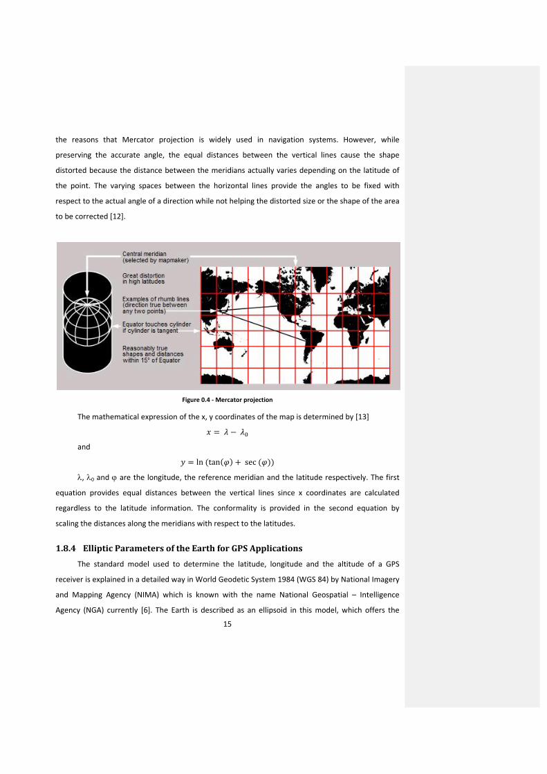
the reasons that Mercator projection is widely used in navigation systems. However, while

preserving the accurate angle, the equal distances between the vertical lines cause the shape

distorted because the distance between the meridians actually varies depending on the latitude of

the point. The varying spaces between the horizontal lines provide the angles to be fixed with

respect to the actual angle of a direction while not helping the distorted size or the shape of the area

to be corrected [12].

Figure 0.4 ‐ Mercator projection

The mathematical expression of the x, y coordinates of the map is determined by [13]

and

ln tan sec

, 0 and are the longitude, the reference meridian and the latitude respectively. The first

equation provides equal distances between the vertical lines since x coordinates are calculated

regardless to the latitude information. The conformality is provided in the second equation by

scaling the distances along the meridians with respect to the latitudes.

1.8.4 Elliptic Parameters of the Earth for GPS Applications

The standard model used to determine the latitude, longitude and the altitude of a GPS

receiver is explained in a detailed way in World Geodetic System 1984 (WGS 84) by National Imagery

and Mapping Agency (NIMA) which is known with the name National Geospatial – Intelligence

Agency (NGA) currently [6]. The Earth is described as an ellipsoid in this model, which offers the

16

cross‐sections parallel to the equator being circular while the ones normal to the equator being

ellipsoid. The semi‐major axis of the ellipsoid, which is normal to the equator and centered at the

center of the Earth is equal to the radius of the equator and is taken 6,378.137 km. The semi‐minor

axis of this ellipsoid, the so‐called polar radius of the Earth, is 6,356.7523142 km according to WGS

84.

1.9 Internal Vehicle Sensors

In vehicle positioning or relative distance measurement, using GPS is usually not enough to

get accurate results [14]. As mentioned in 1.7.4, GPS receivers suffer from many errors caused by

different sources. In order to reduce the errors in the calculations, other inputs are introduced to the

system and combined with a sensor fusion algorithm. These inputs are the information received

from the internal sensors those expected to have a positive effect on the results. The sensors are

already sending information to the relevant parts of the system in the vehicle through CAN bus and

using this connection; the necessary information is forwarded to our sensor fusion system as well.

The sensors those are utilized in the system are listed and described in this chapter.

1. Vehicle Speed over Ground

Vehicle speed over ground is reliable sensor information indicating the instant speed of the

vehicle. It is useful for estimating the position of the vehicle or the distance to an object for a further

time instance.

2. Yaw Rate

Yaw rate is the information received from a sensor, which is able to determine the angular

velocity of the vehicle in degrees/second or radians/second. There are different kinds of sensors

capable of sensing angular velocity using different hardware and software. Yaw rate sensors are

usually considered to be too noisy thereby not very reliable when driving in low speeds. In that case,

steering angle information becomes important to make a better estimation of the actual turning

angle. We also applied a low‐pass‐filter to reduce the noise from the yaw rate information (see

Figure 0.5).

17

Figure 0.5 ‐ Low pass filter applied to yaw rate

3. Reversed Gear

Reversed gear is the indicator for the gear position, which is important to decide whether the

vehicle is moving forward or backward.

Table 3 ‐ Properties of sensor data

Sensor information Data type Min Max Resolution Unit

Vehicle speed float 0 320 0.01 km/h

Yaw rate float -75 74.9998 0.03663 /sec

Gear level boolean 0 1

1.10 Sensor Fusion Systems

A sensor fusion system is a system that combines information from different sources to

achieve the least noisy result possible. The reason behind the necessity of sensor fusion systems in

18

many applications is the fact that each sensor has its own strengths and weaknesses, therefore one

sensor is usually not reliable itself.

There are different methods and algorithms such as Kalman Filtering, Bayesian Networks,

Dempster‐Shafer Theory etc. used to implement a sensor fusion system for different applications

[15]. The strengths and weaknesses of each input are introduced to these algorithms and the

reliability of each input is determined according to the working conditions and the output is

optimized by this way. In this thesis work, a Kalman Filter is used for improving position and distance

measurements.

1.10.1 Inertial Navigation System

Inertial navigation system is a navigation that computes the further position of an object from

the given initial position using motion sensors such as speed and rotation according to the laws of

physics [16]. Every new position is calculated from the previously determined position by a process

known as dead reckoning. It is used in a wide range of applications including aircraft, spacecraft,

submarine, ship, mobile land vehicle and human navigation.

Due to the nature of this system the new position is always dependent on the previous one,

therefore the errors included in the previous calculations are also preserved in the new ones.

1.10.2 Kalman Filter

One of the most well‐known methods for data/sensor fusion algorithms is the Kalman filter,

which is named after Rudolf E. Kalman who proposed a linear data filtering algorithm in his famous

paper (Kalman 1960) in 1960 [17]. The problem to which the Kalman filter finds a solution is

estimating the optimum state of a linear dynamic equation corrupted by white noise using relevant

measurements also containing white noise [18]. It is considered to be one of the biggest discoveries

in statistical estimation theory and has been studied widely for various applications since its

discovery.

In principle, the Kalman filter has two distinguished steps consisting of prediction and

correction [17]. In prediction, the states of the dynamics equation are estimated with a prediction

noise using pre‐defined dynamic model of the process usually being a law of physics. The correction

step has the measurements of these states with a measurement noise. Prediction and measurement

noises are both normally distributed white noises and one should note that they are independent

19

from each other. The Kalman filter improves the predicted state using the measurement with a

weighted gain, which is calculated according to the noise covariance values [19].

Figure 0.6 ‐ Visualization of the Kalman gain

The Kalman filter algorithm

The Kalman filter does not require keeping the history of observations or estimations since it

is a recursive algorithm, which calculates the current estimation only from the latest estimated state

and the current observation. As mentioned in the introduction of the Kalman filter 1.10.2, the

algorithm can be divided into two parts where in the first one, the so‐called prediction step, the

state is estimated from the previous time instance using a linear prediction equation; thereby the a

priori estimate of the state at the current time instance is computed. The a priori estimate is

improved with a noisy measurement feedback in the next step that is known as the correction step.

The specific formulas for these steps are presented below [17].

Priori state estimate

Priori prediction error covariance

Residual

Residual covariance

Kalman gain

Posteriori state estimate

Posteriori prediction error covariance

where;

A is the state transition model,

B is the control‐input model,

u is the control vector,

Prediction

Correction

20

Q is the process error covariance,

z is the measurement,

H is the measurement transition model,

R is the measurement error covariance,

I is the unit matrix.

21

MATHEMATICAL MODEL OF ALGORITHMS AND CONFIGURATION

In this section, the implementation details of our work will be presented with the

mathematical equations defined and the algorithm flow‐charts. Furthermore, solutions to certain

problems such as synchronization and dynamic signal quality detection are presented.

1.11 Overview of the Algorithm

The algorithms that we developed during this thesis work can be divided into three main

parts: information extraction, data synchronization and sensor fusion system. After the information

was simultaneously logged from the CAN bus and the GPS receivers in the two vehicles, first the

necessary data such as speed, yaw rate, latitude, longitude, SNR values and etc. were extracted by

the MATLAB codes we developed. However, neither in between the cars nor in the individual cars

among the GPS and the vehicle sensors, the information was synchronized; therefore, the next step

was synchronizing all the information. The detailed explanation of the way we followed in this part is

given in 1.11.1. Once the data is synchronized, two sensor fusion algorithms can work

simultaneously for the two cars and they can share the necessary information with each other

during the process shown below.

22

1.11.1 Synchronization of GPS and Internal Sensors

In real time applications, data or signal synchronization is one of the most critical aspects that

should be designed and implemented carefully. In our case, although the tests were done offline,

the sensor fusion system requires synchronous information from different inputs in order to process

the output correctly. Moreover, the outputs of the sensor fusion systems running in individual

vehicles are supposed to be synchronous with each other too.

Figure 0.1 ‐ Overview of the sensor fusion system

velocity

direction

velocity

x, y

x, y

direction

Δ , Δ

‐

+

x, y

x, y

R

GPS

gear

gear

speed

speed

Q

Q

filtered yaw rate

filtered yaw rate

yaw rate

yaw rate

Kalman Filter

LPF

50 Hz

50 Hz

1Hz

Kalman Filter

LPF

50 Hz

GPS

R

50 Hz

1Hz

50 Hz

50 Hz

23

The timestamp information of the GPS messages was very sensitive, however there was no

exact match between the absolute time of the GPS and CAN messages. In order to calculate the

exact time difference between them, we took advantage of the cross correlation between the speed

signals received from both inputs. The position of the maximum correlation point with respect to the

reference point gave us the exact time difference between GPS and CAN; therefore, the inputs of the

sensor fusion system were synchronized by considering this difference.

After GPS and CAN signals were synchronized, the vehicles could be synchronized easily using

the timestamps of the signals from two receivers thanks to the precise time information in the GPS

messages.

1.11.2 Parameters of the Kalman Filter

In this section, the actual parameters that were mapped into the formal Kalman filter

algorithm described in 1.10.2 and the initialization of the states will be explained.

States and the transition models of the Kalman filter

The state matrix consists of only the position of the vehicle in our project; therefore, the matrixes

become scalar values. The state and the measurement transition models A and H are both equal to

1.

Δ

where

Δ is 20ms in our system and is the velocity of the vehicle at the precise moment. The detailed

explanation of the derived formulas determining the velocity of the vehicle is given below in this

section.

The priori prediction error covariance becomes

since 1.

As explicitly shown in the previous formula, the process error covariance Q does not

necessarily stay constant throughout the algorithm; contrarily it is updated at every time sample k

by a sub function according to the characteristics of the internal vehicle signals those take part in the

priori estimation step.

24

Once the priori estimates are calculated, the correction step starts with calculating the

residual between the measured and the priori estimated position. One should notice that H was

taken to be 1 earlier. Therefore the residual and the residual covariance are

and

Again, the measurement error covariance R is updated for each new GPS signal by a sub

function, which takes several properties such as number of satellites used in the position calculation

and the Signal to Noise Ratio (SNR) of the signals received from these satellites into account.

The Kalman gain is then calculated by the following equation;

The posteriori state and the prediction error covariance estimations become

and

1

Initialization of the states

The Kalman filter recursively updates the states using the above mentioned formulas.

However, the states should be initialized before the first iteration in order to be updated in the

recursive algorithm.

The easiest way of initializing the states is probably setting all to 0 since they will be updated

later in the process anyway. However, we chose to initialize the position with the first received GPS

coordinates. On the other hand, the prediction error covariance P was set to 5 in the beginning,

which basically means that the first position is assumed to be including an error with a variance of 5

in the Cartesian coordinates.

25

NOYES

NO

NOYES

YES

Start

Read GPS and Sensor

Data

direction = NOT SETInitialize x, Q, P

Do k = 1 to

length of data

direction== SET?

is GPS available?

Is ready to set direction?

direction = SET

Compute S, K, x, P

Compute , Q

= xQ = MAX

Compute

Compute y, R y = 0

R = MAX

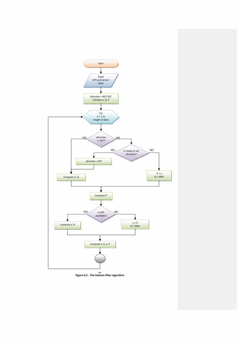
Figure 0.2 ‐ The Kalman filter algorithm

26

Inertial navigation formulas for priori position estimation

The priori position estimate of the vehicle was given as the following above in this section.

Δ

where

is the velocity of the vehicle. However, how the velocity is defined on a specific axis of the

Cartesian coordinate system has not been introduced yet. Obviously considering a two dimensional

Cartesian coordinate system, the velocity on the x or y axis depends on the direction of the vehicle’s

movement. In 1.9, the internal vehicle sensors used in this thesis work were briefly explained and in

this section, the specific formulas using the information from these sensors will be given.

Referring back to 1.9, yaw rate signal gives information on the angular velocity of the vehicle,

which means how many degrees the heading direction of the vehicle will change in a second.

Accordingly, a 0 degrees/second of yaw rate means that the vehicle is heading straight, a 10

degrees/second and ‐5 degrees/second indicate that the vehicle will make an anti‐clock‐wise 10

degrees and a clock‐wise 5 degrees change in its heading direction in one second respectively. If the

current heading direction of the vehicle is known, it is always possible to determine the heading

using the yaw rate information continuously with the following equation.

∆ Ω

Once the direction of the vehicle is computed, the velocity on each axis on the coordinate

system can be calculated by combining the direction with the speed information.

cos

sin

An important point in the velocity calculations is that it is a function of the direction and the

direction is updated recursively by adding the yaw rate at each time, which causes the errors

included in the yaw rate to be added to the direction in a cumulative manner. After a while, the

direction gets highly corrupted because of this motive. In order to reduce this effect, we

implemented a sub function, which periodically keeps track of the two latest positions when the

observations are available and computes the direction of the movement using a simple geometrical

formula shown below.

tan

27

1.11.3 Detection of Signal Qualities for GPS and Internal Sensors

In 1.10.2, it was mentioned that the last decision on the output of the Kalman filter is made by

the Kalman gain factor, which depends on the noise covariance of the prediction and the

observation. Therefore, the key point is introducing the covariance of these processes correctly to

the Kalman filter.

We already cited in 1.11.2 that the error covariance varies by time in both steps. The necessity

behind this variation is the fact that the conditions affecting the noise variance of these processes

actually change by time. For instance, the observation in our system is the position calculated by GPS

receiver and accuracy of this position may change according to the quality of the signal received or

to the number of satellites that were used in calculations at that moment. Additionally the reliability

of the signals received from the vehicle sensors may also alter by the conditions at that moment.

Starting with the quality of the prediction, which is inversely proportional to the noise

variance of the sensors used in our system, which are speed and yaw rate, after careful analysis of

the logged information from these sensors, we deduced that speed could be considered very

accurate all the time, however yaw rate was quite noisy when driving at low speeds up to 20 km/h.

Since the prediction of the position is processing the combined information from both sensors, the

noisy yaw rate data affected the results. Therefore, the covariance of the prediction process Q was a

function of the speed of the vehicle.

On the other hand, it was more complicated to decide on the accuracy of the GPS position due

to the fact that there were many things affecting the calculations such as different noise sources,

number of visible satellites and SNR of the signals received from each satellite.

We discussed in 1.7 that there must be at least three visible satellites to be able to determine

the position of a GPS receiver on the surface of the Earth, and at least four satellites to manage that

with the height information as well. Based on these facts, an idea for estimating the GPS location

accuracy is counting the number of satellite signal SNRs that are higher than a certain threshold.

Using different thresholds to notice the number of satellite signals above those levels was one

method for understanding observation error covariance.

Another method we followed to determine the observation error covariance was calculating

the average SNR of all satellite signals that were used in the position calculations by the receiver.

Since the final result was affected by all the signals received from those satellites, it was practical to

estimate the accuracy of the position using this average SNR. We implemented and tested both

28

methods during our work and although the results were pretty similar, we came to a conclusion that

using average SNR provided slightly better results.

However, we discovered that in certain cases, although the SNR values of the signals were

relatively high, the accuracy of the GPS position could be considerably poor when the vehicle was

driving around tall buildings or passing under obstacles such as bridges. Our guess is multipath

effects caused the results to be corrupted without any significant decrease in the SNR.

1.11.4 Relative Distance Measurement

The final work to be done after determining the positions of the vehicles was measurement of

the relative distance between them. As we mentioned in 1.8.3, Mercator projection was used for

positioning the GPS receiver on a two dimensional plane and the optimization algorithms were done

on this plane.

The difference between the absolute positions on the universal plane only defines the

distance in north‐south and east‐west direction. However, in today’s safety systems, each vehicle

needs to determine the positions of the surrounding vehicles with respect to its own heading angle.

Therefore, each vehicle needs to define a new coordinate system, which is shown in Figure 0.3, sets

the vehicle’s heading angle as the primary horizontal axis indicated with x’. Since the vehicle may

constantly change its heading angle, the coordinate system is updated at every step of the algorithm

and the surrounding vehicles are positioned according to this dynamic coordinate frame

continuously.

The calculations that we made for the relative measurement at a certain time is given as

follows:

∆

∆

tan Δy Δ⁄

α θ

Δ sin

Δ cos

29

Figure 0.3 ‐ Relative distance measurement

30

RESULTS

In order to understand the accuracy, challenges and dependencies of a real time relative

distance measurement system; we did several tests in different areas (urban, suburban) and

environmental conditions (weather, traffic conditions, etc.). Although results from only two tests are

covered comprehensively due to practical reasons, we nevertheless added a table of RMSE and

standard deviation of the errors for each test case at the end of this chapter.

1.12 Test case – 1

This is one of the tests that were done around Chalmers Johanneberg campus area. Below is

the description of this particular test that is studied.

Figure 0.1 ‐ Test track 1

Urban area

Medium traffic

Pursuit (30‐40 meters)

Both cars have varying speeds (15‐40 km/h)

Weather conditions: cloudy and rainy

31

Figure 0.2 ‐ Vehicle speed

Figure 0.3 ‐ Lateral distance

32

Figure 0.4 ‐ Longitudinal distance

Figure 0.5 ‐ Target angle

33

Figure 0.6 ‐ Lateral error histogram

Figure 0.7 ‐ Longitudinal error histogram

34

Figure 0.8 ‐ Target angle error histogram

1.13 Test case – 2

The second test that will be covered in this section was done in a closed traffic path in

countryside. The description of the test is given below.

Countryside

Entry closed to traffic

Pursuit (2.4 sec)

Both cars have varying speeds (60‐80 km/h)

Weather conditions: clear

Path: mostly straight – loop

35

Figure 0.9 ‐ Test track 2

36

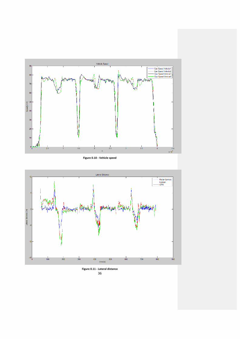
Figure 0.10 ‐ Vehicle speed

Figure 0.11 ‐ Lateral distance

37

Figure 0.12 ‐ Longitudinal distance

Figure 0.13 ‐ Target angle

38

Figure 0.14 ‐ Absolute distance error

Figure 0.15 ‐ Lateral error histogram

39

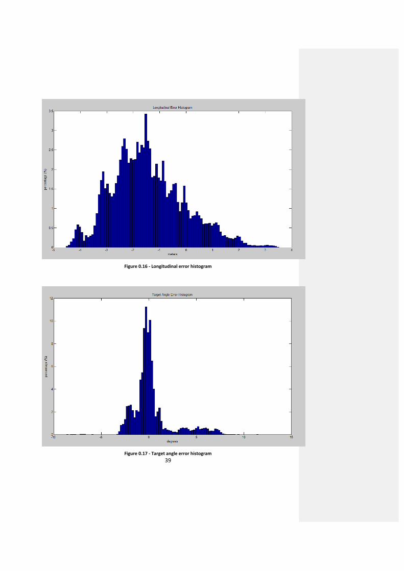
Figure 0.16 ‐ Longitudinal error histogram

Figure 0.17 ‐ Target angle error histogram

40

Table 4 ‐ RMSE and Standard deviation of errors

Case Driving Conditions

RMSE lat (m) Standard

Deviation lat (m)

RMSE lon (m) Standard

Deviation lon (m)

Case 1 Urban Varying

Speed 1.509937 1.463356 2.228135 1.801362

Case 2 Countryside Varying speed

1.369821 1.517508 2.030176 1.814933

Case 3 Urban

Varying Speed 1.483793 1.225087 2.231224 1.803487

Case 4 Countryside

Constant speed 1.019622 0.879626 1.711952 1.317442

Case 5 Countryside Varying speed

1.365131 1.304811 2.314364 2.007950

Case 6 Countryside Varying speed

2.726428 2.671556 2.460274 2.222996

Case 7 Countryside

Constant speed 1.042331 0.892837 1.830348 1.426627

Case 8 Countryside Varying speed

1.631389 1.489401 2.376652 2.114173

Case 9 Urban

Varying Speed 1.529207 1.439083 2.271184 1.940336

Case 10 Countryside Varying speed

1.462437 1.259776 2.189806 1.910531

The results are analyzed and discussed according to the figures and the table above, however

one should consider that error analyses are done with the assumption of perfect accuracy of the

radar‐camera information as mentioned before in 1.5, which is not true in reality.

We have mentioned before that due to the lack of true information on the absolute vehicle

positions; we were only able to do tests when target vehicle was in the field of radar‐camera view.

However, this was not the only problem caused by non‐existence of the true information. Another

thing was the difficulty of determining the error covariance of the GPS receiver positions. Since we

had no information on true positions, we could only use a limited number of experimental

information at known locations and only in immobile situations.

41

RMS errors and standard deviation of the errors show that sensor fusion system with GPS and

vehicle sensors could be a good way for relative distance measurement with around 1.5 and 2.2

meter average lateral and longitudinal RMSE respectively. By using more suitable models in the

sensor fusion system and refining the states of the filter, the errors could be even reduced.

First thing to be noticed from the lateral and longitudinal error histograms (see Figure 0.6,

Figure 0.7, Figure 0.15, Figure 0.16); their patterns do not have normal distribution. Main reason

behind this is the inaccurate models used in the fusion system, which are not optimal for non‐linear

systems. The non‐linearity of the motion and measurement models caused the error distribution to

reshape and have different characteristics. An Extended Kalman Filter, Unscented Kalman Filter or

Particle Filter could provide much better results.

Another interesting point is that the mean of the longitudinal errors is not zero, which we

think was caused by the assumption of constant velocity during one cycle of the fusion system.

However, in reality, the speed of the vehicles had rapid changes at some points of the test drives,

which actually led to varying speeds during a fusion cycle. This behavior changed the mean of the

errors to non‐zero values.

As one of our goals was to understand the noise characteristics of GPS and errors

encountered by the receiver, we spent quite a lot of time to find a correlation between SNR values

of the GPS signals and the positioning errors. However, we could neither end up with certain

thresholds nor could notice distinct behaviors in that sense. In some tests, while the SNR values

were relatively high, the accuracy could still be poor. Interestingly, the opposite scenario was

possible too.

42

Figure 0.18 ‐ GPS clock error

Probably a more marked founding was the difference between two identical GPS receivers.

They could output very different SNR values at the same time, at the same place, which made the

situation even more complicated. On the other hand, one critical GPS receiver error that we noticed

was the clock‐error. In a test drive, we located two same GPS products on one vehicle and wanted to

analyze the behaviors of them. Unexpectedly, there was 1 second difference in the time‐stamps of

two receivers in one particular test (see Figure 0.18). Considering the fact that we heavily relied on

the time‐stamp information of GPS, it is possible that we might have encountered the same

problems when they were positioned in different vehicles, which was impossible to notice in the

current design.

In summary, the results are not as good as it could be because of the simpler design choices,

but even in these conditions they could be considered encouraging. Better suited models and better

understanding of the GPS error distribution could improve the results significantly.

43

CONCLUSION AND FUTURE WORK

Considering the importance of the safety systems in road traffic, collision avoidance systems

are most likely going to be improved continuously. Environmental awareness will always be one of

the key figures in these systems, therefore relative distance measurements will be an important

feature and much more studies and developments should be expected.

The results obtained from our studies showed that it is practical to share GPS and sensor

information between the vehicles to accomplish relative positioning. However; although relative

position estimations have reasonable accuracy, we are not sure how much of the error was

eliminated using the differential equation defined in 1.1, since we do not know the extent of the

error in the absolute positions due to the lack of true position information.

First thing that might be refined to improve relative positions is the vehicle dynamics model

that is used in sensor fusion algorithm. There are already more accurate models used in cars for

different applications such as stability control, etc. The model used in our system is ignoring all the

factors that affect the raw movement such as weight and road slip.

Secondly, the sensor fusion algorithm we used in the calculations is actually not the optimal

solution for non‐linear vehicle motion model and measurement model. The results could be

improved notably with a more suitable algorithm.

We used radar‐camera information as reference since we did not have another option, but it

could actually be introduced to the sensor fusion system as well as with other potentially useful

sensors, so that the combined results could be improved even more.

Finally, many more tests and analyses should be done to get a better understanding of the

noise sources, dependencies of the problem and increase the accuracy of results.

44

BIBLIOGRAPHY

1. IEEE. IEEE 802.11 Official Timelines. [Online]

http://grouper.ieee.org/groups/802/11/Reports/802.11_Timelines.htm.

2. Vehicle Applications of Controller Area Network. Johanson, Karl Henrik, Törngren, Martin

and Nielsen, Lars.

3. GmbH, Vector Informatic. Vector User Manual. 2006.

4. Mohinder S. Grewal, Lawrence R. Weill, Angus P. Andrews. Global Positioning Systems,

Inertial Navigation, and Integration. 2001.

5. Gps Information ‐ NMEA. [Online] http://gpsinformation.org/dale/nmea.htm#nmea.

6. National Imagery and Mapping Agency, Department of Defence. World Geodetic System

1984 (WGS 84). 2000.

7. The Geodetic Survey Section of Survey and Mapping Office. [Online]

www.geodetic.gov.hk/smo/gsi/data/ppt/NMEAandRTCM.ppt.

8. State Water Resources Control Board. [Online]

http://www.swrcb.ca.gov/water_issues/programs/swamp/docs/cwt/guidance/6120.pdf.

9. Stovall, Sherryl H. Basic Inertial Navigation. s.l. : Navigation and Data Link Section ‐ System

Integration Branch, 1997.

10. Elliott D. Kaplan, Christopher J. Hegarty. Understanding GPS ‐ Principles and Applications

Second Edition. 2006.

11. Understanding Coordinate Reference Systems, Datums and Transformations. Janssen, V.

2009.

12. Pennstate College of Earth and Mineral Sciences. Nature of Geometric Information.

[Online] https://www.e‐education.psu.edu/natureofgeoinfo/c2_p29.html.

13. Snyder, John P. Map Projections ‐ A Working Manual. 1987.

14. Tohid Ardeshiri, Sogol Kharrazi, Jonas Sjöberg, Jonas Bärgman, Mathias Lidberg. Sensor

Fusion for Vehicle Positioning in Intersection Active Safety Applications. 2006.

15. Martin E. Liggins, David L. Hall, James Llinas. Handbook of Multisensor Data Fusion,

Theory and Practice, Second Edition. 2009.

16. Woodman, Oliver J. An introduction to inertial navigation. 2007.

17. Greg Welch, Gary Bishop. An Introduction to the Kalman Filter. 2001.

45

18. Mohinder S. Grewal, Angus P. Andrews. Kalman Filtering: Theory and Practice Using

MATLAB Second Edition. 2001.

19. James L. Crawley, Yves Demazeau. Principles and Techniques for Sensor Data Fusion.

20. http://www.swrcb.ca.gov/water_issues/programs/swamp/docs/cwt/guidance/6120.pdf.

[Online]

46

APPENDIX A. SOURCE CODES

A.1 CAN Data Extractor Script

% This script extracts the relevant data from vehicle CAN bus % including internal sensors and radar/camera fused data. close all clear all clc % Get the local time before extraction starts t0 = clock; % Set file folder and file name to read fileFolder = '..\\LogFiles\\'; fileName = 'Aug_20_CAN2_Case02.asc'; fullFileName = [fileFolder fileName]; % Read the file CANFile = fopen(fullFileName, 'rt'); % Requested signals messageID1 = '71B'; funcHandle1 = @extract_radar_71B; messageID2 = '321'; funcHandle2 = @extract_hs_can_speed; % messageID3 = '83'; % funcHandle3 = @extract_hs_can_gear; % messageID4 = '94'; % funcHandle4 = @extract_hs_can_steering; messageID5 = '155'; funcHandle5 = @extract_hs_can_yaw; messageID6 = '600'; funcHandle6 = @extract_radar_yaw; messageID7 = '71C'; funcHandle7 = @extract_radar_71C; messageID8 = '160'; funcHandle8 = @extract_hs_can_revgear; % messageID9 = '321'; % funcHandle9 = @extract_hs_can_acceleration; % Initialize indexes for each vector

47

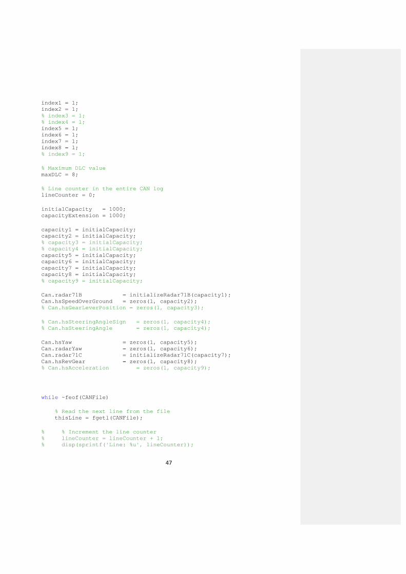
index1 = 1; index2 = 1; % index3 = 1; % index4 = 1; index5 = 1; index6 = 1; index7 = 1; index8 = 1; % index9 = 1; % Maximum DLC value maxDLC = 8; % Line counter in the entire CAN log lineCounter = 0; initialCapacity = 1000; capacityExtension = 1000; capacity1 = initialCapacity; capacity2 = initialCapacity; % capacity3 = initialCapacity; % capacity4 = initialCapacity; capacity5 = initialCapacity; capacity6 = initialCapacity; capacity7 = initialCapacity; capacity8 = initialCapacity; % capacity9 = initialCapacity; Can.radar71B = initializeRadar71B(capacity1); Can.hsSpeedOverGround = zeros(1, capacity2); % Can.hsGearLeverPosition = zeros(1, capacity3); % Can.hsSteeringAngleSign = zeros(1, capacity4); % Can.hsSteeringAngle = zeros(1, capacity4); Can.hsYaw = zeros(1, capacity5); Can.radarYaw = zeros(1, capacity6); Can.radar71C = initializeRadar71C(capacity7); Can.hsRevGear = zeros(1, capacity8); % Can.hsAcceleration = zeros(1, capacity9); while ~feof(CANFile) % Read the next line from the file thisLine = fgetl(CANFile); % % Increment the line counter % lineCounter = lineCounter + 1; % disp(sprintf('Line: %u', lineCounter));

48

[tempToken, tempString] = strtok(thisLine); tempTime = str2double(tempToken); if tempTime >= 0 [tempToken, tempString] = strtok(tempString); tempChannel = str2num(tempToken); if ~isempty(tempChannel) && ishex(strtok(tempString)) [tempMessageID, tempString] = strtok(tempString); % Get data bytes from the current line DataBytes = getDataBytes(thisLine); % Is it Message 1? if strcmp(tempMessageID, messageID1) if index1 == capacity1 Can.radar71B = extendRadar71B(Can.radar71B, ... capacityExtension); capacity1 = capacity1 + capacityExtension; end [Can.radar71B.targetRangeAcceleration(index1), ... Can.radar71B.targetRangeRate(index1), ... Can.radar71B.detectionSensor(index1), ... Can.radar71B.detectionStatus(index1), ... Can.radar71B.targetRange(index1), ... Can.radar71B.targetMotionClass(index1), ... Can.radar71B.targetId(index1), ... Can.radar71B.targetWidth(index1), ... Can.radar71B.targetMoveableStatus(index1), ... Can.radar71B.targetAngle(index1)] ... = funcHandle1(DataBytes); index1 = index1 + 1; % Is it Message 2? elseif strcmp(tempMessageID, messageID2) if index2 == capacity2 Can.hsSpeedOverGround = [Can.hsSpeedOverGround ... zeros(1, capacityExtension)]; capacity2 = capacity2 + capacityExtension; end Can.hsSpeedOverGround(index2) = funcHandle2(DataBytes); index2 = index2 + 1; % % Is it Message 3? % elseif strcmp(tempMessageID, messageID3) % if index3 == capacity3 % Can.hsGearLeverPosition = [Can.hsGearLeverPosition ... % zeros(1, capacityExtension)]; % capacity3 = capacity3 + capacityExtension; % end % Can.hsGearLeverPosition(index3) = funcHandle3(DataBytes);

49

% index3 = index3 + 1; % Is it Message 4? % elseif strcmp(tempMessageID, messageID4) % if index4 == capacity4 % Can.hsSteeringAngleSign = [Can.hsSteeringAngleSign ... % zeros(1, capacityExtension)]; % Can.hsSteeringAngle = [Can.hsSteeringAngle ... % zeros(1, capacityExtension)]; % capacity4 = capacity4 + capacityExtension; % end % [Can.hsSteeringAngleSign(index4), ... % Can.hsSteeringAngle( index4)] = funcHandle4(DataBytes); % index4 = index4 + 1; % Is it Message 5? elseif strcmp(tempMessageID, messageID5) if index5 == capacity5 Can.hsYaw = [Can.hsYaw ... zeros(1, capacityExtension)]; capacity5 = capacity5 + capacityExtension; end Can.hsYaw(index5) = funcHandle5(DataBytes); index5 = index5 + 1; % Is it Message 6? elseif strcmp(tempMessageID, messageID6) if index6 == capacity6 Can.radarYaw = [Can.radarYaw ... zeros(1, capacityExtension)]; capacity6 = capacity6 + capacityExtension; end Can.radarYaw(index6) = funcHandle6(DataBytes); index6 = index6 + 1; % Is it Message 7? elseif strcmp(tempMessageID, messageID7) if index7 == capacity7 Can.radar71C = extendRadar71C(Can.radar71C, ... capacityExtension); capacity7 = capacity7 + capacityExtension; end [Can.radar71C.targetRangeAcceleration(index7), ... Can.radar71C.targetRangeRate(index7), ... Can.radar71C.detectionSensor(index7), ... Can.radar71C.detectionStatus(index7), ... Can.radar71C.targetRange(index7), ... Can.radar71C.targetMotionClass(index7), ... Can.radar71C.targetId(index7), ... Can.radar71C.targetWidth(index7), ... Can.radar71C.targetMoveableStatus(index7), ... Can.radar71C.targetAngle(index7)] ... = funcHandle7(DataBytes); index7 = index7 + 1;

50

% Is it Message 8? elseif strcmp(tempMessageID, messageID8) if index8 == capacity8 Can.hsRevGear = [Can.hsRevGear ... zeros(1, capacityExtension)]; capacity8 = capacity8 + capacityExtension; end Can.hsRevGear(index8) = funcHandle8(DataBytes); index8 = index8 + 1; % % Is it Message 9? % elseif strcmp(tempMessageID, messageID9) % if index9 == capacity9 % Can.hsAcceleration = [Can.hsAcceleration ... % zeros(1, capacityExtension)]; % capacity9 = capacity9 + capacityExtension; % end % Can.hsAcceleration(index9) = funcHandle9(DataBytes); % index9 = index9 + 1; end end end end Can.radar71B = removeAppendedFromRadar71B(Can.radar71B, index1 - 1); Can.hsSpeedOverGround = Can.hsSpeedOverGround(1 : index2 - 1); % Can.hsGearLeverPosition = Can.hsGearLeverPosition(1 : index3 - 1); % Can.hsSteeringAngleSign = Can.hsSteeringAngleSign(1 : 2 : index4 - 1); % Can.hsSteeringAngle = Can.hsSteeringAngle(1 : 2 : index4 - 1); Can.hsYaw = Can.hsYaw(1 : index5 - 1); Can.radarYaw = Can.radarYaw(1 : index6 - 1); Can.radar71C = removeAppendedFromRadar71C(Can.radar71C, index7 - 1); Can.hsRevGear = Can.hsRevGear(1 : index8 - 1); % Can.hsAcceleration = Can.hsAcceleration(1 : index9 - 1); % Close the file fclose(CANFile); % Set the name of the binary file to save variables matFileName = ['..\\Resources\\' fileName(1:end-3) 'mat']; % Save the variables save(matFileName, 'Can'); % Calculate elapsed time for all process elapsedTime = etime(clock, t0); elapsedMinutes = floor(floor(elapsedTime) / 60);

51

elapsedSeconds = elapsedTime - (elapsedMinutes * 60); disp(sprintf('Elapsed time for the operations: %2u min %5.2f sec\n', ... elapsedMinutes, elapsedSeconds));

A.2 GPS Data Extractor Script

% This script extracts the relevant data from GPS logs. close all clear all clc for gpsNo = 1:1 for caseNo = 2:3 % Set GPS file folder and file name fileFolder = '..\\LogFiles\\'; fileName = sprintf('Aug_20_GPS%d_Case%02d.txt', gpsNo, caseNo); fullFileName = [fileFolder fileName]; % Read GPS file gpsFile = fopen(fullFileName, 'rt'); % Initialize the index for each different message indexGPRMC = 1; indexGPGGA = 1; indexGPGSA = 1; indexGPGSV = 1; % Initialize GPGSV Struct for first time call to the function Gps.gpgsv.elevation = 0; Gps.gpgsv.azimuth = 0; Gps.gpgsv.snr = 0; Gps.gpgsv.satPrnNo = 0; % Flag Identifiers for GPGSV message LAST_MESSAGE_GPGSV = 1; NOT_LAST_MESSAGE_GPGSV = 0; % Index of the message IDs messageIdIndex = 1:6; % Extract GPS Information until the end of the file while ~feof(gpsFile) % Read the next line gpsline = fgets(gpsFile); if ~isempty(find(gpsline == '*', 1))

52

% Is it GPRMC? if strcmp('$GPRMC', gpsline(messageIdIndex)) % Extract GPRMC message [Gps.gprmc.type( indexGPRMC, :), ... Gps.gprmc.time( indexGPRMC, :), ... Gps.gprmc.status( indexGPRMC, :), ... Gps.gprmc.latitude( indexGPRMC ), ... Gps.gprmc.longitude(indexGPRMC ), ... Gps.gprmc.speed( indexGPRMC ), ... Gps.gprmc.angle( indexGPRMC ), ... Gps.gprmc.date( indexGPRMC, :)] ... = extract_GPS_gprmc(gpsline); indexGPRMC = indexGPRMC + 1; % Is it GPGGA? elseif strcmp('$GPGGA', gpsline(messageIdIndex)) % Extract GPGGA message [Gps.gpgga.type( indexGPGGA, :), ... Gps.gpgga.time( indexGPGGA, :), ... Gps.gpgga.latitude( indexGPGGA ), ... Gps.gpgga.longitude( indexGPGGA ), ... Gps.gpgga.fixQuality(indexGPGGA ), ... Gps.gpgga.noOfSat( indexGPGGA )] ... = extract_GPS_gpgga(gpsline); indexGPGGA = indexGPGGA + 1; % % Is it GPGSA? % elseif strcmp('$GPGSA', gpsline(messageIdIndex)) % % % Extract GPGSA message % Gps.gpgsa(indexGPGSA) = extract_GPS_gpgsa(gpsline); % indexGPGSA = indexGPGSA + 1; % Is it GPGSV? elseif strcmp('$GPGSV', gpsline(messageIdIndex)) % Extract GPGSV message [Gps.gpgsv, flag] = extract_GPS_gpgsv(gpsline, ... Gps.gpgsv, ... indexGPGSV); % Was it the last message? if flag == LAST_MESSAGE_GPGSV % Increase the index indexGPGSV = indexGPGSV + 1; end end end end

53

% Close the file fclose(gpsFile); % Set the name of the binary file to save variables matFileName = ['..\\Resources\\' fileName(1:end-3) 'mat']; % Save the variables save(matFileName, 'Gps'); clear Gps end end

A.3 Synchronization of GPS and CAN

function [Can, Gps] = synchronizeCanGps(Can, Gps) % This function synchronizes the CAN and GPS messages by applying cross % correlation on the speed signals received from both inputs. % Length determination lengthCan_ = length(Can.hsSpeedOverGround); lengthGps_ = length(Gps.gprmc.speed); % Synchronization setup estimatedPoint_ = max(lengthGps_, lengthCan_); corrResult_ = xcorr(Gps.gprmc.speed, Can.hsSpeedOverGround); [maxVal_ maxPoint_] = max(corrResult_); shifting_ = estimatedPoint_ - maxPoint_; % Synchronization of Gps and Can information if shifting_ < 0 Gps = removeFirstNFromGps(Gps, -shifting_); else Can = removeFirstNFromCan(Can, shifting_); end return

A.4 Mercator Projection

function [x_, y_] = getMercator(lat_, lon_) % This function calculates the mercator projection from the given % geographic coordinates. x_ = lon_; y_ = rad2deg(log(tand(lat_) + secd(lat_))); return

54

A.5 Heading Update to Remove Bias in Yaw Rate

function heading_ = updateHeading(Can_, Y_, X_, k_) % This function updates the heading of a car using previous positions. % Function should be called periodically to reduce the effects of yaw bias. % Get distance in x and y coordinates between two previous consecutive % positions when GPS signal received. y = Y_(k_ - 50) - Y_(k_ - 100); x = X_(k_ - 50) - X_(k_ - 100); % Calculate heading of the vehicle heading_ = atand(y / x); % If the angle is supposed to be in the 2nd or 3rd zone of the % Cartesian coordinate system? if x < 0 heading_ = heading_ - 180; end % Add the heading change from the last time instant till now. heading_ = mod(heading_ + sum(20e-3 .* Can_.hsYaw(k_-49:k_)), 360); return

A.6 Main Script for Sensor Fusion

close all clear all clc % Case details month = 'Aug'; day = 6; caseNo = 11; % Folder to access logged information fileFolder = '..\Resources\'; % Load synchronized GPS and CAN data from both vehicles load([fileFolder sprintf('%s_%02d_GPS1_Case%02d_N.mat', month, day, caseNo)]); load([fileFolder sprintf('%s_%02d_CAN1_Case%02d_N.mat', month, day, caseNo)]); load([fileFolder sprintf('%s_%02d_GPS2_Case%02d_N.mat', month, day, caseNo)]); load([fileFolder sprintf('%s_%02d_CAN2_Case%02d_N.mat', month, day, caseNo)]); % Common length of the arrays len = length(Can1.hsYaw);

55

% Copy the latitude and longitude information to arrays lat1Gps = Gps1.gpgga.latitude; lon1Gps = Gps1.gpgga.longitude; lat2Gps = Gps2.gprmc.latitude; lon2Gps = Gps2.gprmc.longitude; % Static memory allocation for the arrays % Priori states Lat1Hat = zeros(1, len); Lon1Hat = zeros(1, len); Lat2Hat = zeros(1, len); Lon2Hat = zeros(1, len); % Posteriori states Lat1Opt = zeros(1, len); Lon1Opt = zeros(1, len); Lat2Opt = zeros(1, len); Lon2Opt = zeros(1, len); Y1Opt = zeros(1, len); X1Opt = zeros(1, len); Y2Opt = zeros(1, len); X2Opt = zeros(1, len); % Pre-defined error covariance values for different reliability levels FULL_TRUST = 2 * 10e-5; HIGH_TRUST = 5 * 10e-5; HALF_TRUST = 10 * 10e-5; LOW_TRUST = 15 * 10e-5; NO_TRUST = 30 * 10e-5; % Prediction processes error covariances P1 = HALF_TRUST; P2 = HALF_TRUST; % Initialize the direction of the cars % 0 -> East % 90 -> North % 180 -> West % -90 -> South direction1 = 0; % Case 1 -> -1 direction2 = 0; % Case 1 -> 20 % Preprocessor constants for direction set SET = 1; NOT_SET = 0; % Reset direction set flags for the cars directionFlag1 = NOT_SET; directionFlag2 = NOT_SET;

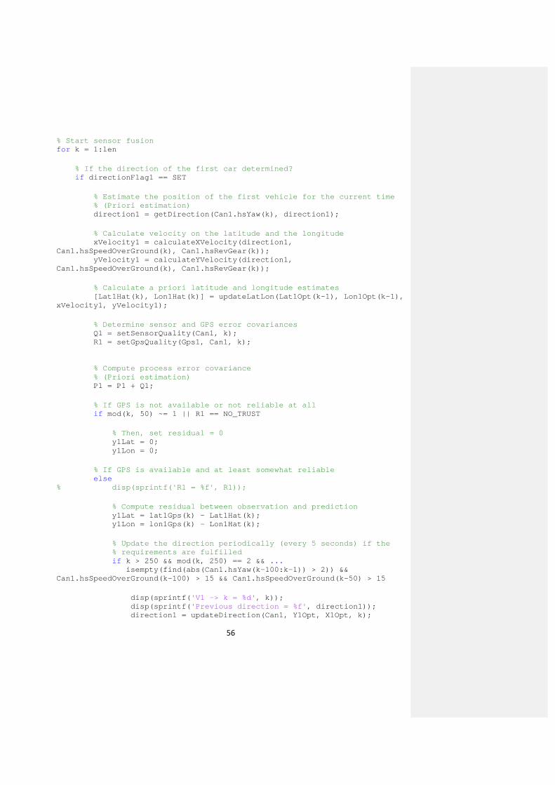
56

% Start sensor fusion for k = 1:len % If the direction of the first car determined? if directionFlag1 == SET % Estimate the position of the first vehicle for the current time % (Priori estimation) direction1 = getDirection(Can1.hsYaw(k), direction1); % Calculate velocity on the latitude and the longitude xVelocity1 = calculateXVelocity(direction1, Can1.hsSpeedOverGround(k), Can1.hsRevGear(k)); yVelocity1 = calculateYVelocity(direction1, Can1.hsSpeedOverGround(k), Can1.hsRevGear(k)); % Calculate a priori latitude and longitude estimates [Lat1Hat(k), Lon1Hat(k)] = updateLatLon(Lat1Opt(k-1), Lon1Opt(k-1), xVelocity1, yVelocity1); % Determine sensor and GPS error covariances Q1 = setSensorQuality(Can1, k); R1 = setGpsQuality(Gps1, Can1, k); % Compute process error covariance % (Priori estimation) P1 = P1 + Q1; % If GPS is not available or not reliable at all if mod(k, 50) ~= 1 || R1 == NO_TRUST % Then, set residual = 0 y1Lat = 0; y1Lon = 0; % If GPS is available and at least somewhat reliable else % disp(sprintf('R1 = %f', R1)); % Compute residual between observation and prediction y1Lat = lat1Gps(k) - Lat1Hat(k); y1Lon = lon1Gps(k) - Lon1Hat(k); % Update the direction periodically (every 5 seconds) if the % requirements are fulfilled if k > 250 && mod(k, 250) == 2 && ... isempty(find(abs(Can1.hsYaw(k-100:k-1)) > 2)) && Can1.hsSpeedOverGround(k-100) > 15 && Can1.hsSpeedOverGround(k-50) > 15 disp(sprintf('V1 -> k = %d', k)); disp(sprintf('Previous direction = %f', direction1)); direction1 = updateDirection(Can1, Y1Opt, X1Opt, k);

57

disp(sprintf('Updated direction = %f\n', direction1)); end end % Update measurement error covariance S1 = P1 + R1; % Calculate Kalman Gain K1 = P1 / S1; % Correct the estimated position % (Posteriori estimation) Lat1Opt(k) = Lat1Hat(k) + K1 * y1Lat; Lon1Opt(k) = Lon1Hat(k) + K1 * y1Lon; % Update the error covariance % (Posteriori estimation) P1 = (1 - K1) * P1; % If the direction is not determined yet? else % disp(sprintf('V1 -> Flag Not Set! k = %d', k)); % Posteriori estimation is equal to the measurement Lat1Opt(k) = lat1Gps(k); Lon1Opt(k) = lon1Gps(k); % Check if the direction can be determined now? if k > 4*50 && isReadyToSetDirection(Can1, Gps1, k) direction1 = setDirection(Gps1, k); directionFlag1 = SET; end end % Get Mercator projected coordinates [X1Opt(k), Y1Opt(k)] = getMercator(Lat1Opt(k), Lon1Opt(k)); % If the direction of the first car determined? if directionFlag2 == SET % Estimate the position of the second vehicle for the current time % (Priori estimation) direction2 = getDirection(Can2.hsYaw(k), direction2); % Calculate velocity on the latitude and the longitude xVelocity2 = calculateXVelocity(direction2, Can2.hsSpeedOverGround(k), Can2.hsRevGear(k)); yVelocity2 = calculateYVelocity(direction2, Can2.hsSpeedOverGround(k), Can2.hsRevGear(k)); % Calculate a priori latitude and longitude estimates

58

[Lat2Hat(k), Lon2Hat(k)] = updateLatLon(Lat2Opt(k-1), Lon2Opt(k-1), xVelocity2, yVelocity2); % Determine sensor and GPS error covariances Q2 = setSensorQuality(Can2, k); R2 = setGpsQuality(Gps2, Can2, k); % Compute process error covariance % (Priori estimation) P2 = P2 + Q2; % If GPS is not reliable at all? if mod(k, 50) ~= 1 || R2 == NO_TRUST % Residual = 0 y2Lat = 0; y2Lon = 0; else % disp(sprintf('R2 = %f', R2)); % Compute residual between measurement and prediction y2Lat = lat2Gps(k) - Lat2Hat(k); y2Lon = lon2Gps(k) - Lon2Hat(k); % Update the direction periodically if the requirements are % fulfilled if k > 250 && mod(k, 250) == 2 && ... isempty(find(abs(Can2.hsYaw(k-100:k-1)) > 2)) && Can2.hsSpeedOverGround(k-100) > 15 && Can2.hsSpeedOverGround(k-50) > 15 disp(sprintf('V2 -> k = %d', k)); disp(sprintf('Previous direction = %f', direction2)); direction2 = updateDirection(Can2, Y2Opt, X2Opt, k); disp(sprintf('Updated direction = %f\n', direction2)); end end % Update measurement error covariance S2 = P2 + R2; % Calculate Kalman Gain K2 = P2 / S2; % Correct the estimated position % (Posteriori estimation) Lat2Opt(k) = Lat2Hat(k) + K2 * y2Lat; Lon2Opt(k) = Lon2Hat(k) + K2 * y2Lon; % Update the error covariance % (Posteriori estimation) P2 = (1 - K2) * P2; % If the direction is not determined yet?

59

else % Posteriori estimation is equal to the measurement Lat2Opt(k) = lat2Gps(k); Lon2Opt(k) = lon2Gps(k); % Check if the direction can be determined now? if k > 4*50 && isReadyToSetDirection(Can2, Gps2, k) direction2 = setDirection(Gps2, k); directionFlag2 = SET; end end % Get Mercator projected coordinates [X2Opt(k), Y2Opt(k)] = getMercator(Lat2Opt(k), Lon2Opt(k)); % Difference between radar detection range and distance of the actual GPS receiver positions GpsBetwRadarLength = 5.1; navigationDist(k) = calcDist(Lat1Opt(k), Lon1Opt(k), Lat2Opt(k), Lon2Opt(k)); RelativeDist(k) = navigationDist(k) - GpsBetwRadarLength; if Can2.hsSpeedOverGround(k) == 0 estRadarAngle(k) = 0; else estRadarAngle(k) = calculateAngleBetweenCars(X1Opt(k), Y1Opt(k), X2Opt(k), Y2Opt(k), direction2); end end [LatDistFromRadar, LonDistFromRadar] = calcLatLongDistance(((Can2.radar71B.targetAngle(13:end))),Can2.radar71B.targetRange(13:end)); [LatDistFromKalman, LonDistFromKalman] = calcLatLongDistance(estRadarAngle(1:end-12), RelativeDist(1:end-12)); [RMSE_LAT, RMSE_LON, STD_LAT, STD_LON] = calcErrorStatistics(LatDistFromRadar, LatDistFromKalman, LonDistFromRadar, LonDistFromKalman); disp(sprintf('rmse Lateral = %f\nrmse Longitudinal = %f\n', RMSE_LAT, RMSE_LON)); disp(sprintf('std Lateral = %f\nstd Longitudinal = %f\n', STD_LAT, STD_LON)); ARRAY_START = 1; ARRAY_SIZE = len-12; timeAxis = 20e-3 * [0:ARRAY_SIZE - ARRAY_START];

60

erasedLatDist = LatDistFromKalman; erasedLatDist(find(Can2.radar71B.targetRange(13:end) == 0)) = NaN; LatDistFromRadar(find(Can2.radar71B.targetRange(13:end) == 0)) = NaN; figure plot(timeAxis, LatDistFromRadar(ARRAY_START:ARRAY_SIZE)); hold on plot(timeAxis, erasedLatDist(ARRAY_START:ARRAY_SIZE), 'r'); legend('Radar-Camera', 'Kalman'); xlabel('time (s)'); ylabel('Lateral distance (m)'); title('Lateral Distance'); erasedLonDist = LonDistFromKalman; erasedLonDist(find(Can2.radar71B.targetRange(13:end) == 0)) = NaN; LonDistFromRadar(find(Can2.radar71B.targetRange(13:end) == 0)) = NaN; figure plot(timeAxis, LonDistFromRadar(ARRAY_START:ARRAY_SIZE)); hold on plot(timeAxis, erasedLonDist(ARRAY_START:ARRAY_SIZE), 'r'); legend('Radar-Camera', 'Kalman'); xlabel('time (s)'); ylabel('Longitudinal distance (m)'); title('Longitudinal Distance'); radarTargetAngle = Can2.radar71B.targetAngle(13:end); erasedAngle = estRadarAngle; erasedAngle(find(Can2.radar71B.targetRange(13:end) == 0)) = NaN; radarTargetAngle(find(Can2.radar71B.targetRange(13:end) == 0)) = NaN; figure plot(timeAxis, radarTargetAngle(ARRAY_START:ARRAY_SIZE)); hold on plot(timeAxis, erasedAngle(ARRAY_START:ARRAY_SIZE), 'r'); legend('Radar-Camera', 'Kalman'); xlabel('time (s)'); ylabel('angle (degrees)'); title('Target Angle'); [LatHist, LatError] = hist(LatDistFromRadar(ARRAY_START:ARRAY_SIZE) - erasedLatDist(ARRAY_START:ARRAY_SIZE), 100); [LonHist, LonError] = hist(LonDistFromRadar(ARRAY_START:ARRAY_SIZE) - erasedLonDist(ARRAY_START:ARRAY_SIZE), 100); [AngHist, AngError] = hist(radarTargetAngle(ARRAY_START:ARRAY_SIZE) - erasedAngle(ARRAY_START:ARRAY_SIZE), 100); LatHist = (LatHist / sum(LatHist)) * 100; LonHist = (LonHist / sum(LonHist)) * 100; AngHist = (AngHist / sum(AngHist)) * 100; figure; bar(LatError, LatHist, 1.0); title('Lateral Error Histogram'); xlabel('meters'); ylabel('percentage (%)');

61

figure; bar(LonError, LonHist, 1.0); title('Longitudinal Error Histogram'); xlabel('meters'); ylabel('percentage (%)'); figure; bar(AngError, AngHist, 1.0); title('Target Angle Error Histogram'); xlabel('degrees'); ylabel('percentage (%)');