thesis reservoir simulation
TRANSCRIPT

8/10/2019 Thesis Reservoir Simulation
http://slidepdf.com/reader/full/thesis-reservoir-simulation 1/87
Reservoir simulation with imposed uxcontinuity conditions on heterogeneous and
anisotropic media for general geometries, andthe inclusion of hysteresis in forward modeling
Dr.Scient Thesis, Reservoir Mechanics
Geir Terje Eigestad
Department of MathematicsUniversity of Bergen
24th April 2003

8/10/2019 Thesis Reservoir Simulation
http://slidepdf.com/reader/full/thesis-reservoir-simulation 2/87

8/10/2019 Thesis Reservoir Simulation
http://slidepdf.com/reader/full/thesis-reservoir-simulation 3/87
For my sister Monica

8/10/2019 Thesis Reservoir Simulation
http://slidepdf.com/reader/full/thesis-reservoir-simulation 4/87
8/10/2019 Thesis Reservoir Simulation
http://slidepdf.com/reader/full/thesis-reservoir-simulation 5/87
Preface
This thesis constitutes the work that I have done during the time as a Dr. Sci-ent. student at the Department of Mathematics, University of Bergen (UiB). It iswritten in accordance with the criteria stated by the University Board. The work has been done in collaboration with the research group at Norsk Hydro and theDepartment of Mathematics at University of Bergen.
Magne Espedal (UiB) and Ivar Aavatsmark (UiB/Norsk Hydro ResearchCentre) have been advisors for me, and Norsk Hydro has provided the fundingfor the work.
The thesis’ main research part is the ve papers A-E, and four of these havebeen published in conference proceedings and journals. The main focus of thesepapers is on issues related to reservoir simulation with improved reliability, and inparticular discretization methods which should be valid for complex geometry.
The governing equations for uid ow in oil and gas reservoirs can beclassied according to conventional theory of applied mathematics. This doesnot mean that all issues regarding reservoir simulation have been solved. Reliablereservoir simulation is a complicated eld, and many issues are still notknown to asatisfactory level. The oil and gas reservoirs are very complex physical media, andthe level of heterogeneity seen in real sandstones can sometimes overwhelm thenovice mathematician. Sandstones may have rapidly varying structure, porosityand permeability on a small scale. It can sometimes be hard to convince oneself that it is possible to model enormous amounts of uids on a large scale when beingfaced with such complexity.
Regardless of these complexities, applied reservoir simulation does studymovement of uids in complex media. The goal for scientists is to include as muchinformation as possible in the models for both the uid ow as well as the physicalmedia themselves. At multi discipline research centres, geologists, geophysicists,
physicists and mathematicians work together with this drive. Each group maywork with their own ’small’ problem, but all these pieces should eventually bewoven together. For the most complex reservoirs one might never be able toperform accurate and detailed predictions of the future performance. But beingable to see ’the main trends’ is very useful, and this is really the goal even the

8/10/2019 Thesis Reservoir Simulation
http://slidepdf.com/reader/full/thesis-reservoir-simulation 6/87
scientist should aim for.The contributions in this thesis are mainly in the mathematical and numer-
ical modelling of uid ow in oil and gas reservoirs. For a person not directlyinvolved, even the eld of numerical modelling may seem like a very narrowissue to focus on, and merely a detail in the big picture of oil exploration andproduction. We, however argue that this is not the case. For future predictionof the performance of an oil reservoir, one has to build a mathematical model.This model should be reliable for a wide range of input, such as rock types, welldata, uid composition etc. Although there will always be uncertainty involvedwith such parameters, the bottom line for numerical modelling should be that themodels give us reliable output for cases that can be veried.
For most of the work in this thesis, the physical parameters that describe thereservoir are assumed to be given. The issue of reliable parameter determinationis a eld of it’s own, and when these are known, the techniques of numericalmodelling/discretisation might be applied to more complex input.
Part I of the thesis gives an introduction to reservoir simulation and theissues that I have been working with. Part II is a collection of research papers thathave been written during the PhD period.

8/10/2019 Thesis Reservoir Simulation
http://slidepdf.com/reader/full/thesis-reservoir-simulation 7/87
Outline of Thesis
The thesis is divided into two main parts. Part I gives an overview and summaryof the theory that lies behind the ow equations and the discretisation principlesused in the work. Part II is a collection of research papers that have been writtenby the candidate (in collaboration with others).
The main objective of this thesis is the discretisation of an elliptic PDE whichdescribes the pressure in a porous medium. The porous medium will in generalbe described by permeability tensors which are heterogeneous and anisotropic. Inaddition, the geometry is often complex for practical applications. This requiresdiscretization approaches that are suited for the problems in mind. The discret-isation approaches used here are based on imposed ux and potential continuity,and will be discussed in detail in Chapter 3 of Part I. These methods are calledMulti Point Flux Approximation Methods, and the acronym MPFA will be usedfor them. Issues related to these methods will be the main issue of this thesis.
The rest of this thesis is organised as follows:
Part I : Chapter 1 gives a brief overview of the physics and mathematics
behind reservoir simulation. The standard mass balance equations are presented,and we try to explain what reservoir simulation is. Some standard discretizationsmethods are briey discussed in Chapter 2.
The main focus in Part I is on the MPFA discretisation approach for variousgeometries, and is given in Chapter 3. Some details may have been left out in thepapers of Part II, and the section serves both as a summary of the discretisationmethod(s), as well as a more detailed description than what is found in the papers.
In Chapter 4, extensions to handle time dependent and nonlinear problems arediscussed. Some of the numerical examples presented in Part II deal with twophase ow, and are based on the extension given in this chapter.
Chapter 5 discusses numerical results that have been obtained for the MPFAmethods for elliptic problems, and Chapter 6 deals with issues related to propertiesof the discrete set of (one phase) pressure equations.
Chapter 7 contains summaries of the research papers found in Part II.

8/10/2019 Thesis Reservoir Simulation
http://slidepdf.com/reader/full/thesis-reservoir-simulation 8/87
Part II : This part contains 5 research papers. The papers mainly deal withMPFA methods, and issues related to the discrete set of equations that areobtained by these discretisation methods. Also, one of the papers (Paper E) dealswith the inclusion of hysteresis for forward simulation of two phase ow. Thetheme in Paper E is therefore also related to discretisation issues.
The papers included in Part II are:
Paper A: Symmetry and M-matrix Issues for the MPFA O-method onan Unstructured Grid . Published in Computational Geosciences , Volume 6,Editors M. G. Edwards, R. D. Lazarov, I. Yotov.
Paper B: MPFA applied to Irregular grids and Faults . Published in De-velopments in Water Sciences Volume 47 , Editors: Hassanizadeh, Schotting,Gray, Pinder.
Paper C: MPFA for Faults with Crossing Layers and Zig-zag Patterns .In Proceedings of ECMOR VIII , 2002.
Paper D: A note on convergence of the MPFA O-method; numerical ex-periments on some 2D and 3D grids . Draft manuscript.
Paper E: Numerical Modeling of Capillary Transition Zones . SPE 64374, inProceedings of the SPE APOGCE, 2000.

8/10/2019 Thesis Reservoir Simulation
http://slidepdf.com/reader/full/thesis-reservoir-simulation 9/87
Acknowledgements
This work would never have been completed without the help of my advisorsMagne Espedal and Ivar Aavatsmark. I owe them a big thank for their guidanceand encouragement throughout this time. I would especially thank Magne for hispositiveness and ability to make me perform more even in the hardest situations.Ivar needs a big thank for sharing his deep insight in many issues in the eldof applied mathematics. They also both deserve my gratitude for their ability tohandle my moods during times of intense stress.
During the time as a PhD student many people have been helpful and goodto talk to. At Norsk Hydro Research Centre, I would like to thank the followingpeople: Edel Reiso, Hilde Reme, Rune Teigland and Tor Barkve. Formerly em-ployed Johne Alex Larsen has also been good support. The management of Norsk Hydro needs a big thank for funding the work.
At CSIRO Division of Petroleum Resources, Dr. Chris Dyt and Dr. CedricGrifths deserve my thanks for letting me stay there for 6 months in 2000/2001.I would also thank Professor Thomas Russell for letting me stay at University of Colorado at Denver for three weeks during spring 2002.
At the Mathematical Institute I have had very good colleagues. I want to thank Erlend Øian for many interesting discussions regarding reservoir simulation andimplementation. Jan Martin Nordbotten is also a good source of inspiration. HansFredrik Nordhaug has been of tremendous help in all Latex issues, and all generalcomputer questions. His attitude to questions is admirable even when the answeris trivial. I would also like to thank Torbjørn Aadland and Jarle Hauk˚ as for lettingme use parts of their C++ code.
Helge Dahle is a very nice person to have at the department; both academicallyand personally. I want to thank him for good discussions and taking me and otherPhD students hunting and hiking near his cabin.
Runhild Klausen has been a good friend and colleague. I would like to thank
her for a good cooperation in the academic eld and her friendliness at all times.My family has been fantastic to me all my life, including my period as PhD
student. They have always supported me, and it has been good to retire to themwhen the times have been hard.

8/10/2019 Thesis Reservoir Simulation
http://slidepdf.com/reader/full/thesis-reservoir-simulation 10/87
My loving wife Melanie is the one who made this possible. Without her Iwould never even have started doing a PhD. I owe her all my love.
Geir Terje EigestadBergen, April 2003.

8/10/2019 Thesis Reservoir Simulation
http://slidepdf.com/reader/full/thesis-reservoir-simulation 11/87
Contents
I Introduction 1
1 Basics 31.1 Darcy’s law . . . . . . . . . . . . . . . . . . . . . . . . . . . . . 41.2 Multiphase ow . . . . . . . . . . . . . . . . . . . . . . . . . . . 51.3 Capillary pressure; inclusion of hysteresis . . . . . . . . . . . . . 71.4 Geology . . . . . . . . . . . . . . . . . . . . . . . . . . . . . . . 9
2 Discretisation methods; various formulations 112.1 Finite Differences . . . . . . . . . . . . . . . . . . . . . . . . . . 112.2 Finite element methods . . . . . . . . . . . . . . . . . . . . . . . 122.3 Mixed nite element methods . . . . . . . . . . . . . . . . . . . 14
3 Multi Point Flux Approximation methods 173.1 Transmissibility calculations . . . . . . . . . . . . . . . . . . . . 173.2 Unstructured grids; 2D polygonal CVs . . . . . . . . . . . . . . . 253.3 Faults with crossing grid lines . . . . . . . . . . . . . . . . . . . 283.4 Treatment of Dirichlet boundary conditions . . . . . . . . . . . . 34
4 Time dependent problems 394.1 Nonlinearities . . . . . . . . . . . . . . . . . . . . . . . . . . . . 39
5 Numerical results 415.1 Analytical solutions . . . . . . . . . . . . . . . . . . . . . . . . . 43
6 Properties of discrete system 456.1 M-matrices . . . . . . . . . . . . . . . . . . . . . . . . . . . . . 46
6.2 Notes on violation of maximum principle . . . . . . . . . . . . . 46
7 Summary of the papers 497.1 Summary of Papers A and B . . . . . . . . . . . . . . . . . . . . 497.2 Summary of paper C . . . . . . . . . . . . . . . . . . . . . . . . 52

8/10/2019 Thesis Reservoir Simulation
http://slidepdf.com/reader/full/thesis-reservoir-simulation 12/87
0
7.3 Summary of paper D . . . . . . . . . . . . . . . . . . . . . . . . 547.4 Summary of paper E . . . . . . . . . . . . . . . . . . . . . . . . 55
8 Further work 57
Bibliography 59
II Published and submitted work 65
A Symmetry and M-matrix issues for the O-method on an UnstructuredGrid 67
B MPFA applied to Irregular Grids and Faults 69
C MPFA for Faults with Crossing Layers and Zig-zag Patterns 71
D A note on convergence of the MPFA O-method; numerical experi-ments on some 2D and 3D grids 73
E Numerical Modeling of Capillary Transition Zones 75

8/10/2019 Thesis Reservoir Simulation
http://slidepdf.com/reader/full/thesis-reservoir-simulation 13/87
Part I
Introduction

8/10/2019 Thesis Reservoir Simulation
http://slidepdf.com/reader/full/thesis-reservoir-simulation 14/87

8/10/2019 Thesis Reservoir Simulation
http://slidepdf.com/reader/full/thesis-reservoir-simulation 15/87
Chapter 1
Basics
Reservoir simulation is the study of how uids ow or behave in a reservoir. Areservoir is a porous medium where hydrocarbons exist in the pore space, and in
the oil industry the goal is to determine how hydrocarbons and water ow/behavein a reservoir under different conditions.To do so, one has to derive mathematical and physical models for the pro-
cesses that occur in the reservoir. Often the physical processes themselves areof interest, and many physical phenomena (such as ’interface-interaction’ whendifferent phases are present, and complexities associated with hysteresis) are notfully understood. This thesis approaches reservoir simulation from a mathemat-ical point of view, and some physical assumptions must be made to complete themathematical approach. The theory that leads to the partial differential equations(PDEs) that describe the uid ow in a porous medium, is standard in many text-books in the area of reservoir simulation, and further theory details may be foundin for example Aziz [39].
For simulation of uid ow in a hydrocarbon reservoir (eg. to quantify howmuch of a specic uid ows through a specic area of a reservoir due to pressuredifferences), one has to solve a set of coupled PDEs. This set of equations is oftenthe starting point for applied mathematics, and discretisation of the equations isa eld that has received a lot of attention in the past decades. The PDEs arisefrom the principle of mass conservation and a physical description of the velo-city/ux dependency of the pressure (Darcy’s law). Commonly studied are themass conservation equations for each of the uid phases present in a reservoir. Init’s original form, the mass conservation equation for a uid with mass density m
(mass per volume) and uid density ρ on a domainΩ
is given by
Ω
∂∂t
mdV + ∂Ωρv · n dS = Ω
qdV . (1.1)
Here v is the volumetric ow density of the uid, n is the outward normal
8/10/2019 Thesis Reservoir Simulation
http://slidepdf.com/reader/full/thesis-reservoir-simulation 16/87
4 Basics
vector of the surface ∂Ω , and q is a source term. In other words; Eq. (1.1) saysthat the accumulation of mass of the uid within a volume Ω is balanced by theuxes (across the edges of the volume) and possible sources q . Eq. (1.1) is anintegral equation. The integral form of the mass balance equation(s) will be used
throughout this thesis. A discretisation approach based on the integral form iscalled a Control Volume (CV) formulation. We will use this form because of theadvantage that local mass conservation is satised.
When applied to a porous medium, we need to dene the porosity of the me-dium/rock. This is the fraction of the volume of the rock where mobile uid mayexist, and will be denoted φ . Hence, we may formally dene it by
φ =V p
V c, (1.2)
where V p is the effective pore volume available for the uid, and V c is the totalvolume of the rock. The total pore volume of a rock may be larger than V p, butthis extra volume is not ’connected’ to the pore space where uids may ow. Itshould be mentioned that a typical sand stone found in reservoirs from the NorthSea has a porosity of 10-20 percent.
The mass density for a representative volume is hence ρφ . Applying thistogether with the divergence theorem, we obtain the integral form of the massconservation equation for a single phase uid within a volume Ω V of a porousmedium
Ω V
(∂(ρφ )
∂t+ ∇· (ρv ) − q ) dV = 0. (1.3)
This equation is referred to as the single phase ow equation, or the singlephase pressure equation. The reason for it’s name is that with some further as-sumptions discussed below (Darcy’s law + density function of pressure), this is aintegral PDE where only the pressure needs to be treated as an unknown.
1.1 Darcy’s law
The French engineer Henry Darcy experimented with ow through different typesof sand during the 19th century. In a range of experiments with ow vertically
through samples of sand, he concluded that the ow through the sands was pro-portional to the pressure difference between the top and bottom pressure. This lawis now known as Darcy’s law. In it’s most primitive form (1D, single phase, grav-ity neglected), the relation says that the volumetric ow density (Darcy velocity)v is proportional to the gradient of the pressure p:

8/10/2019 Thesis Reservoir Simulation
http://slidepdf.com/reader/full/thesis-reservoir-simulation 17/87
1.2 Multiphase ow 5
v = − k∂p∂x
. (1.4)
The proportionality constant k is called the permeability or conductivity of the medium. For ow in higher dimensions, the permeability will be a (spatiallyvarying) tensor K , and when gravity is included, Darcy’s law for single phase owreads
v = − K (∇ p + ρg∇ d ). (1.5)
This may now be inserted in Eq. (1.3), and pressures will hence enter theequation. If it is assumed that the uid at all times occupy the pore space, weobtain a parabolic PDE which states how the pressure varies in space and time:
Ω V
(∂(ρφ )
∂t−∇· (ρK (∇ p + ρg∇ d )) − q )dV = 0. (1.6)
If the uid further is assumed to be incompressible, the rst term will vanish.When no sources or sinks are present, one hence obtains a purely elliptic pressureequation (time independent)
− ∂Ω∇· (K ∇ u) = 0. (1.7)
where we have dened the potential u of the uid through the relation
∇ u = ∇ p + ρg∇ d . (1.8)
When suitable boundary conditions are posed, Equation (1.7) has a unique solu-tion.Whereas reservoir simulation rarely is as simple as to solve time independent
problems, many discretisation methods that are applied for time dependent prob-lems, are based on the purely elliptic equation. Time discretisation is briey dis-cussed in Chapter 4, and is often included by a standard backward Euler schemefor time dependent terms.
Most of the work in this thesis (papers A-D) uses Eq. (1.7) as the basis for thediscretisations to be dealt with.
1.2 Multiphase owWhen several phases or components are present in a porous medium, mass con-servation must be posed for each of the phases or components. In reservoir simu-lation, there are usually 3 phases that may exist; oil, gas and water. In the Black

8/10/2019 Thesis Reservoir Simulation
http://slidepdf.com/reader/full/thesis-reservoir-simulation 18/87
6 Basics
Oil formulation, hydrocarbons will be grouped, and either be classied as gas oroil. Heavy components will be grouped as oil, and lighter components will begrouped as gas components. Depending on temperature, density and pressure,lighter hydrocarbons may exist in both oil and gas phase. This means that the gas
components may exist in either oil or gas phase. The water component will onlyexist in the water phase.For the oil and water component respectively, the mass conservation equation
is given by.
Ω V
(∂(ρ i S iφ )
∂t−∇ · (
k ri
µ iρ iK ∇ ui ))dV = Ω V
q i , i = o, w. (1.9)
For the gas component, the mass conservation equation is slightly differentbecause the component may exist both in oil and gas phase, and we refer to for in-stance [40] for details. Eq. (1.9) is a parabolic type of equation, which contains anelliptic term (second term on left hand side). Although each mass balance equa-tion is parabolic, the total system of mass balance equations has a more hyperboliccharacter. This is for instance discussed in [52]. The new quantities S i , k ri and µ i
of Eq. (1.9) will be explained in the following: If the three components/phasesoil, gas and water exist in our system, three mass conservation equations must besolved in the region we investigate. The efcient pore space will be assumed tobe lled with uid at all times. Depending on the processes, the different phaseswill compete to occupy this space. It is then natural to dene phase saturations.By this we mean the ratio of the available pore space the different phases occupy.Formally, the saturation of phase i in a representative volume V is dened as
S i =V iV , (1.10)
where V i is the volume occupied by the specic phase. Hence, the saturations varybetween 0 and 1. Since the phases compete to occupy pore space, the effectivepermeabilities will be reduced, and this is reected in the occurrence of the entitiesk ri , of Eq. (1.9). These entities are called relative permeabilities , k ri , and will bereduction factors of the permeability K . The relative permeabilities are functionswhich depend on the saturation of phase i, ie. k ri = k ri (S i ). They take valuesbetween 0 and 1.
For hysteresis models, the relative permeabilities also depend on the directionof the ow processes, as discussed in the next subsection.
The entity µ i is called the viscosity of the phase i. This is a weakly nonlinearterm, and for many applications the viscosities of pure uids will be treated asconstants. For gases, simple models use the linear relationship
µg = bp . (1.11)

8/10/2019 Thesis Reservoir Simulation
http://slidepdf.com/reader/full/thesis-reservoir-simulation 19/87
1.3 Capillary pressure; inclusion of hysteresis 7
The quantity b will be a gas dependent constant. For a three phase system the threesaturations will be unknowns of the three equations of the form (1.9). In additionto this, each of the three phase pressures will be unknowns. As densities, ρ i , arealso assumed to depend on the pressures, the total number of unknowns in the
three coupled mass conservation equations is 6. To close the system of equations,three closure relations are needed.One closure relation is intuitive if the pore space is lled with uids at all
times:
S i = 1, i = w, o,g , (1.12)
where the different subscripts denote water, oil and gas respectively. To get thetwo remaining closure conditions, one needs to know more about the physics of multiphase interactions. Moreover, to make the system of mass balance equationssolvable, the physics must be quantied.
1.3 Capillary pressure; inclusion of hysteresis
In black oil models, it is commonly assumed that the phase pressures are re-lated through a quantity called the capillary pressure. When only two phasesare present, the capillary pressure is given by the pressure difference between thenon-wetting uid and the wetting uid:
P c = pnw − pw . (1.13)
For two phase problems in the oil industry this may be oil and water, or gasand water. If all three phases (water, oil and gas) exist, two capillary pressures willbe used; the capillary pressure between oil and water and the capillary pressurebetween gas and oil:
P cow = po − pw, P cgo = pg − po. (1.14)
Experimental results show that P cow is (mainly) a function of the water satura-tion (S w), and that P cgo is (mainly) a function of the gas saturation ( S g ). The twocapillary pressure relationships then close the system of equations obtained whenmodelling three phase ow. Since the capillary pressure and the relative permeab-
ilities of Eq. (1.9) depend on the solutions S i , the set of mass balance equationsare nonlinear (with respect to solution variables).
Much emphasis is made in experimental reservoir physics to describe the ca-pillary pressure behaviour. In addition to being dependent on the water saturation,the capillary pressure description also depends on whether a phase is entering or

8/10/2019 Thesis Reservoir Simulation
http://slidepdf.com/reader/full/thesis-reservoir-simulation 20/87
8 Basics
Figure 1.1: Primary drainage capillary pressure curve with imbibition capillarypressure curves starting out from different points on the primary drainage curve.
exiting the pore space. In physics this is referred to as irreversible processes or
hysteresis .When water (wetting phase) enters the pore space, this is called imbibition,
and when oil (non-wetting phase) enters the pore space this is called drainage.In Paper E in Part II of this thesis, a consistent capillary pressure and relative
permeability hysteresis model is included for forward modelling of two phase owin a reservoir. The idea is that the uid ow simulator should dynamically updatecapillary pressure and relative permeabilities according to what direction the owhas. For reasons explained in the paper, the reservoir will be initialised with a(single) primary drainage capillary pressure curve prior to production from thereservoir. Figure 1.1 illustrates possible imbibition curves that may start out fromthe primary drainage curve.
If pure imbibition takes place in a reservoir, the capillary pressure time evolu-tion will be described by imbibition curves. When gravity is included in a model,and the system is assumed to be in vertical equilibrium, the capillary pressurewill vary linearly with height, and different grid cells at different height start outwith different saturations. This means that even for pure imbibition throughoutthe reservoir, different capillary pressure descriptions apply for different parts of the reservoir. Such cases have been investigated in Paper E. The model allows fordifferent capillary pressure curves for all grid cells. In addition to (primary andsecondary) imbibition curves, arbitrary secondary drainage curves may apply forthe different cells throughout the simulation. Examples of such curves are visual-
ised in Fig. 1.2a. Here we depict examples of capillary pressure scanning curvesfor cells that have their origin at some point of the primary drainage curve. InFig. 1.2b relative permeability scanning curves are visualised, and are explainedas follows: A cell may have an initial water saturation corresponding to the satur-ation at point (1). If imbibition starts for this cell, the relative permeability curve

8/10/2019 Thesis Reservoir Simulation
http://slidepdf.com/reader/full/thesis-reservoir-simulation 21/87
1.4 Geology 9
a. Capillary pressure. b. Relative permeability
1
2
Figure 1.2: a: Capillary pressure scanning curves. Scanning curves are closedloops, and arbitrary reversals may occur within the loops. b: Relative permeabilityscanning curves.
will follow the lowermost path to point (2). If the direction of the ow is reversedat point (2), the relative permeability curve will follow a different path back to(1). Notice that the loop between (1) and (2) is closed; this is an experimentalobservation, and is included in the scanning curve generation.
Similar explanations may be given for the curves of Fig. 1.2a, and details maybe found in Paper E.
1.4 Geology
Reservoir simulation has become very advanced over the past decades. This is dueto at least two main reasons. The rst reason is of course the computer revolu-tion, which allows large models to be implemented for computing. The secondreason is that the geology of a North Sea reservoir may often be known quite ac-curately (compared to other porous media). Simulation grids may then be verylarge, and the level of details can be very high. Figure 1.3 shows the simulationgrid for a realistic eld example. One of the reasons for the high level of de-tails is the considerable effort which is put into seismic measuring prior to drillingexploration wells. Also, the history may be well known for a reservoir that hasbeen producing hydrocarbons for many years (5-15 years) through logging and
measured production etc. This again may be used to verify or recalculate geo-physical data. Parameter estimation is an important area in it’s own, and produc-tion data is essential to recalculate/calibrate a model with respect to porosity andpermeability. Because the geology may be known at such a detailed level, onemay be required to model ow on grids that include faults and general complex

8/10/2019 Thesis Reservoir Simulation
http://slidepdf.com/reader/full/thesis-reservoir-simulation 22/87
10 Basics
Figure 1.3: Simulation grid for realistic North Sea eld example
Figure 1.4: Extracted part of sandstone found in the Oslo Fault.
geometry. Complex geometry has been a key issue in the work of this thesis. Pa-pers B and C discuss MPFA discretisation for simulation grids where faults havebeen included. Faults may be observed and studied in ’analogues’ to North Seareservoirs. One examples of such an analogue may be found in the Oslo Fault .Such analogues may be useful for understanding the ow mechanisms in faultsand fractures. Also, they support the need to model uid ow on simulation gridswhich contain faults, have large aspect ratios and grid cells that may degenerate
to triangles/tetrahedra.A part of some sandstone found in the Oslo Fault is visualised in Fig. 1.4,where the scale is ’a few meters’. Even on this small scale the permeability mayvary extensively.

8/10/2019 Thesis Reservoir Simulation
http://slidepdf.com/reader/full/thesis-reservoir-simulation 23/87
Chapter 2
Discretisation methods; variousformulations
Discretisation of the governing equations for uid ow has been the issue of manyresearchers involved in porous media ow. Finite difference methods (FD) havebeen used extensively in commercial reservoir simulation, whereas nite elementmethods (FEM) have a strong support in applied mathematics.
We will here briey describe the following methods: (Control volume) nitedifferences, nite element- and mixed nite element methods.
The starting point for the discretisation methods to be discussed is the purelyelliptic equation, which is obtained when a possible source q has been added inEq. (1.7):
−∇ · (K ∇ u) = q . (2.1)
Suitable boundary conditions will also apply, and for reservoir simulation thesewill usually be no-ow at boundaries, ie. K ∇ u · n at the boundary ∂Ω of somedomain Ω .
2.1 Finite Differences
Finite difference based discretisation (FD) is used extensively in conventionalreservoir simulation. The basic idea is to approximate derivatives by discrete dif-ferences. In 1D the use of nite difference approximations for the elliptic equation
(2.1) is justied since the permeability K = k then is a scalar entity.For 1D, the second order problem u = f may be discretised by applying the
forward discretisation for the rst derivative u (x ) = (u(x + h) − u(x ))/ h , whichleads to a similar treatment of u (x ). For multi dimensional problems with non-orthogonal grids and general tensor permeability description, such differences are

8/10/2019 Thesis Reservoir Simulation
http://slidepdf.com/reader/full/thesis-reservoir-simulation 24/87
12 Discretisation methods; various formulations
not directly applicable to Eq. (2.1), as the differentiation involves the permeabilityas well as the pressure. The 1D version of Eq. (2.1) is
∂∂x
(k (x )∂u (x )
∂x) = 0, (2.2)
so that differentiation of the permeability must also be ’included’. Denoting F =k ∂u
∂x , the discrete version of (2.2) takes the form ( F (x + h) − F (x ))/ h . Withoutgoing into detail, there are possible grids to use for nite difference discretisations:point- or cell distributed grids. Cell centred grids (non-uniform) are preferableto use because they yield local mass conservation, and have consistent uxes.This is enforced through harmonic averages of permeabilities obtained at mediadiscontinuity points. It should be noted that the FD discretisation on cell centredgrid in 1D is second order convergent [34], even though the discretisation schemeis inconsistent.
For 2D orthogonal grids where the principal axes of the permeability tensorsare aligned with the coordinate axes, the 1D principles may be utilised to ob-tain discretisation schemes on cell centred grids. Such grids will be termed K -orthogonal grids. Convergence on cell centred grids is proven in [34] and [26].
For general non-orthogonal grids in 2D, and generally varying permeabilitytensors, direct nite difference discretisation does not lead to convergent schemes.The numerical solutions convergence to the wrong solution, and this may in somecases be interpreted as convergence to solutions for continuous problems wherethe permeability tensors are not symmetric. The MPFA discretisation methodsto be discussed in Chapter 3 will be able to handle full tensor representation of the permeabilities and non-orthogonal grids. Our numerical results (eq. PaperD) indicate/show convergence for examples with skew grids and full permeability
tensor description.
2.2 Finite element methods
We will here briey discuss the variational formulation of the problem (2.1), andthe use of nite element methods to discretise the equation.
The equation −∇ · (K ∇ u) = q can be rewritten in order to obtain a weak for-mulation of the equation: take the original equation, multiply by a suitable test function of some function space V [47], and integrate over a domain Ω :
− Ω(∇ · (K ∇ u)vdσ = Ω
qvdσ . (2.3)
Eq. (2.3) may be rewritten by using the rules for partial integration:
ΩK ∇ u ·∇ vdσ − ∂Ω
K ∇ u · nvdS = Ωqvdσ . (2.4)

8/10/2019 Thesis Reservoir Simulation
http://slidepdf.com/reader/full/thesis-reservoir-simulation 25/87
2.2 Finite element methods 13
If the boundary conditions are K ∇ u · n = 0 at ∂Ω , the second term of the left handside vanishes, and the variational equation reads
Ω
K ∇ u ·∇ vdσ =
Ω
qvdσ , ∀v ∈V . (2.5)
This type of boundary condition is called a natural boundary condition, whereasit is possible to dene boundary conditions for the functions v ∈V by v = 0 on∂Ω . The latter boundary condition is called an essential boundary condition. It iscommon to use the notation ( ·, ·) for inner products in some inner product space,see for example [47]. Letting ( ·, ·) here denote the inner product in the innerproduct space L 2(Ω ), we may rewrite Eq. (2.5) as
(K ∇ u,∇ v) = (q , v), ∀v ∈H 1(Ω ), (2.6)
The solution of Eq. (2.3) will be denoted a weak solution of the original equation(2.1). One hence wants to solve this equation for u. The equivalence of the weak solution and the original solution for smooth K is proven in various textbookson nite element analysis, see for example [47] and [50]. The equivalence of the weak solution and the solution of the integral equation − ∇ · (K ∇ u) = q is also valid for discontinuous K . Although not discussing discontinuous K , theequivalence of the solutions is discussed in [48] for solutions with regularity lessthan H 2.
The term ( K ∇ u,∇ v) of Eq. (2.6) is a bilinear form , see [47]. Since K is sym-metric, this bilinear form will be symmetric . The bilinear form will be bounded (orequivalently continuous ) provided that K is bounded ( K ∈L ∞ (Ω )). Further, thebilinear form will be coercive because of the positive deniteness of K . Existenceand uniqueness of a solution u of Eq. (2.6) is then proven by the Lax-Milgramtheorem [47].
To solve a discrete problem of the form (2.6), one may choose a nite-dimensional subspace V h ⊂H 1. The discrete problem then reads: nd uh ∈V hsuch that
(K ∇ uh ,∇ v) = (q ,v), ∀v ∈V h . (2.7)
This method is called the (Continuous) Galerkin Finite Element Method. Underthe same conditions as above ( V h closed subspace of H 1, (K ∇ uh ,∇ v) bounded,
symmetric bilinear form that is coercive on V h ), there exists a unique uh that solves(2.7). The Galerkin Finite Element Method is an example of a method where thediscrete solution is sought in a subspace V h ⊂V , whereas nonconforming methodsdo not seek a solution in a subspace of V . Discontinuous Galerkin Methods [37]are also methods where jumps in the pressure are allowed.

8/10/2019 Thesis Reservoir Simulation
http://slidepdf.com/reader/full/thesis-reservoir-simulation 26/87

8/10/2019 Thesis Reservoir Simulation
http://slidepdf.com/reader/full/thesis-reservoir-simulation 27/87
2.3 Mixed nite element methods 15
The discrete space P h is the space of piecewise constants (which is a subspaceof L ), and the discrete space V h is in many applications the lowest order RaviartThomas space [27], [28]
The power of the mixed methods lies in the way they are able to handle media
discontinuities. The methods may be shown to be locally mass conservative whenthe media have discontinuities. One of the drawbacks of the method is that thediscrete system of equations is a saddle point problem, which is more costly tosolve than symmetric positive denite systems. In addition, more unknowns needto be solved for.
The mixed nite element framework has also been extended to account for acontrol volume formulation by Russell [29], [30] and coworkers. The ExpandedMixed Finite Element Method was developed by Wheeler, Yotov and coworkers[35], [36]. The relationship between this method and the MPFA O-method wasrecently found by Klausen [32].
The next chapter deals with the MPFA discretisation methods, and are al-ternative discretisation methods to the methods discussed in this chapter.

8/10/2019 Thesis Reservoir Simulation
http://slidepdf.com/reader/full/thesis-reservoir-simulation 28/87

8/10/2019 Thesis Reservoir Simulation
http://slidepdf.com/reader/full/thesis-reservoir-simulation 29/87
Chapter 3
Multi Point Flux Approximationmethods
The main work in this thesis has been on various Multi Point Flux Approximationmethods, and discretisation issues related to these. It is important for a discretisa-tion method to handle complex geometry in order for it to be applied for realisticcases. In addition, the discretisation methods should be applicable in physicalspace if this is required. The MPFA methods have this advantage.
MPFA methods have also been the issue in work by Edwards and coworkers[17], [18] and [19].
We will here give a thorough description of the methods for the geometriesthat have been considered in the papers: 2D quadrilaterals, 2D polygonal con-trol volumes, 3D quadrilaterals with crossing grid lines and handling of generalDirichlet boundary conditions.
3.1 Transmissibility calculations
The basic idea behind the MPFA methods is to dene discrete uxes for edgesof control volumes by a reasonable restriction of the medium. The ideas can becarried out for several types of geometries, and can be illustrated in 2D by thegeneral quadrilateral grid visualised in Fig. 3.1.
In practical reservoir simulation, the geometry may very well have similartrends as in this gure. Fluxes should therefore be calculated for each cell edge,
where the orientation of the different edges may vary highly throughout the grid.Furthermore, the permeability tensor K will be heterogeneous and anisotropic,and the principal directions are likely to vary from grid cell to grid cell. How-ever, K is assumed to be symmetric and positive denite. A ’good’ discretisationmethod should take this physical picture into account, and produce reliable uxes

8/10/2019 Thesis Reservoir Simulation
http://slidepdf.com/reader/full/thesis-reservoir-simulation 30/87
18 Multi Point Flux Approximation methods
Figure 3.1: Possible local gridding situation; grid cells need not be orthogonal.
a. Polygonals b. Triangles
Figure 3.2: Unstructured, conforming 2D grids.
for all cell edges that are encountered.The MPFA approach differs from methods such as FEM (continuous Galerkin
method) [47], and Finite Differences [39], [40] by the fact that the MPFA meth-ods discretise the ux itself, whereas the methods mentioned above discretise thepressure. But the MPFA methods also yield pressure equations to solve instead of ux equations. Mixed nite element methods consider both pressures and uxesas unknowns, as discussed in Sec. 2.3.
We will rst try to give a unied treatment of the ideas that lie behind theMPFA discretisation method for various conforming grids. By conforming gridswe mean grids where corners of grid cells meet other corners. The grid shown inFig. 3.1 is an example of such grids. Some other examples are shown in Fig. 3.2.
As mentioned above, the basic ideas behind the MPFA control-volume formu-lation is to determine uxes across all edges of all grid cells in our grid. Hence,all grid cells are control volumes for which we pose mass conservation. By this
approach local mass conservation will be satised. Further, we want to expressthe edge uxes by some local formula/molecule. In doing so, we dene a corner of degree n at corners where n grid cells meet. This denition goes for both tri-angular, quadrilateral and polygonal control volumes, see Fig. 3.3. The MPFAapproach has also been discussed for non-conforming grids in [6], [7] and [12].

8/10/2019 Thesis Reservoir Simulation
http://slidepdf.com/reader/full/thesis-reservoir-simulation 31/87
3.1 Transmissibility calculations 19
i
Figure 3.3: Left: Interaction region and associated corner for 2D quadrilateralcontrol volumes, degree of corner is 4. Right: Interaction region for polygonalcontrol volumes, degree of corner is 3.
The degree of the corner is dened to be the number of grid cells that meet inthe corner. Around each corner an interaction region is dened, and the interactionregions make up a dual grid to the original control volume grid. The controlvolume grid and associated dual grid for a general conforming 2D quadrilateralgrid is visualised in Fig. 3.4
Figure 3.4: Control volume grid (fully drawn lines) and associated interactionregions (dotted lines).
Here, the interaction regions (indicated by dotted lines) may in general have8 edges, and a particular interaction region is visualised on the left hand side of Fig. 3.3. For some special polygonal control volumes the interaction region maybe a triangle as in the rhs. of Fig. 3.3. The reason why the interaction region has
8 edges for the quadrilateral case is explained by the algorithm for constructingthe interaction regions in Fig. 3.3: From each node we draw (dotted) lines tomidpoints of cell edges, and an octagon arises around each corner. The midpointsof the edges are denoted dividing points or continuity points . The dividing pointsneed not be midpoints of the edges, but for the 2D discussion in this thesis, the

8/10/2019 Thesis Reservoir Simulation
http://slidepdf.com/reader/full/thesis-reservoir-simulation 32/87
20 Multi Point Flux Approximation methods
midpoints of edges are chosen as dividing points/continuity points.For the interaction depicted on the left hand side of Fig. 3.3, four grid cells
meet at the corner associated with the interaction region. There will be four celledges that meet in the corner, and parts of these cell edges will be dened to belong
to the interaction region. These parts will be dened sub-interfaces or half-edges ,and it is these we want to calculate uxes for within the interaction region. Awhole cell edge for both quadrilaterals and general polygonals will be covered bytwo neighbouring interaction regions. The quadrilateral case is depicted in Fig.3.5.
E
III
Figure 3.5: Whole cell edge is covered by two neighbouring interaction regions.Total ux obtained by summing uxes for two half edges. Interaction regions forquadrilateral grid cells depicted.
If the degree of the corner associated with an interaction region is n, we saythat n grid cells interact in the interaction region. The number of interacting cellsdetermine how the ux-molecule for a sub-interface will be. For each sub-interfacethe ux will be a weighted sum of the potentials at the nodes of the cells thatinteract:
f i =n
j = 1
t ij u j . (3.1)
These weights will be denoted transmissibilities , and the discretisation prob-lem for the MPFA control volume method is to determine these. When the gridis quadrilateral, n = 4 in Eq. (3.1), and for the 2D polygonals studied in Paper A,n = 3. We may express the n sub-interface uxes of an interaction region by thegeneral matrix notation
f = T n× nu , (3.2)
where f and u are n × 1 vectors, and T n× n is an n × n matrix. The ux across thewhole cell edge E of Fig. 3.5 is found by summing two half edge uxes of two

8/10/2019 Thesis Reservoir Simulation
http://slidepdf.com/reader/full/thesis-reservoir-simulation 33/87
3.1 Transmissibility calculations 21
neighbouring interaction regions. In total this yields a ux that is a weighted sumof the 6 (node) potential values of the cells that touch upon the whole cell edge.Similarly, the ux for a whole cell edge of the polygonal control volumes (withtriangular interaction regions) discussed in Paper A, is given by a weighted sum
of 4 potential values.Looking at the continuous case, uxes across cell edges are given by
f = − S K ∇ u · n dS . (3.3)
Assume that the ux across sub-interface i of the left interaction region of Fig3.3 is to be considered. If the ux is to be approximated by using the informationto the left of the sub-interface, the gradient of the potential for this cell is needed.By the assumption that the potential is linear for the part of the grid cell containedin the interaction region, ∇ u is hence constant, and the (discrete) ux across thesub-interface will also be constant (see Eq. (3.4) below).
Likewise, the ux may be approximated by the information to the right of thesub-interface, and the two discrete ux expressions should then be equal. Thediscrete ux across the cell edge can hence be expressed as
f i = − n T i K i± ∇ ui± , (3.4)
where the index i± denotes if the ux is approximated by the information of eitherthe cell in the positive or anti-positive direction of the edge (positive directiondened by positive direction of normal vector). If, for instance, the potential wasassumed to be bilinear, uxes would not be constant across cell edges.
Formally, the ux continuity condition for each sub-interface i of an interac-tion region reads
f i,i− = f i ,i+ , (3.5)
The gradient of the potentials in each of the sub-cells contained in an interac-tion region will now be derived in order to use explicit expressions for Eq. (3.4).
Since the potential U is linear on each sub-cell j of the control volume, theequation that describes a potential plane applies:
U j (x ) = ∇U j (x − x 0) + U 0 , (3.6)
where x is the position vector, x 0 is the node of grid cell j , and U 0 is the potentialvalue at the node.
The potentials at the continuity points may be used as the basis for determ-ining the gradient of the potential in each sub-cell of an interaction region. Thisinformation may be inserted in Eq. (3.6) to obtain

8/10/2019 Thesis Reservoir Simulation
http://slidepdf.com/reader/full/thesis-reservoir-simulation 34/87
22 Multi Point Flux Approximation methods
x x ν
ν
0 12
1
−
−2
Figure 3.6: Variational triangle associated with part of quadrilateral controlvolume contained in interaction region; x0 is node of grid cell, x 1 and x 2 arecorresponding dividing points/continuity points
∇U · (x k − x 0) = uk − u0 , k = 1,2. (3.7)
This system may be written as
X ∇U = u1 − u0u2 − u0
, (3.8)
where X is the matrix
X = (x 1 − x 0)T
(x 2 − x 0)T . (3.9)
The inverse of X must hence be found. Inward normal vectors of the vari-ational triangle are introduced:
ν 1 = R (x 2 − x 0), ν 2 = − R (x 1 − x 0), (3.10)
where
R = 0 1− 1 0 . (3.11)
The vectors and points used here are illustrated in Fig. 3.6, where the gradientof the potential is to be determined for a sub-cell of a quadrilateral grid cell. The
matrix R has the property that for vectors a and b, aRb is equal to the thirdcomponent of the cross product between a and b. Moreover, the determinant of X is
T = det (X ) = (x 1 − x 0)T R (x 2 − x 0). (3.12)
8/10/2019 Thesis Reservoir Simulation
http://slidepdf.com/reader/full/thesis-reservoir-simulation 35/87
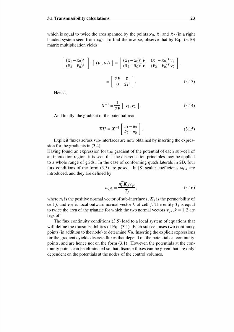
3.1 Transmissibility calculations 23
which is equal to twice the area spanned by the points x 0, x 1 and x 2 (in a righthanded system seen from x0). To nd the inverse, observe that by Eq. (3.10)matrix multiplication yields
(x 1 − x 0)T
(x 2 − x 0)T · (ν 1, ν 2) = (x 1 − x 0)T ν 1 (x 1 − x 0)T ν 2(x 2 − x 0)T ν 1 (x 2 − x 0)T ν 2
.
= 2F 0
0 2F . (3.13)
Hence,
X − 1 = 12F
ν 1, ν 2 . (3.14)
And nally, the gradient of the potential reads
∇U = X − 1 u1 − u0u2 − u0
. (3.15)
Explicit uxes across sub-interfaces are now obtained by inserting the expres-sion for the gradients in (3.4).Having found an expression for the gradient of the potential of each sub-cell of an interaction region, it is seen that the discretisation principles may be appliedto a whole range of grids. In the case of conforming quadrilaterals in 2D, fourux conditions of the form (3.5) are posed. In [8] scalar coefcients ω ijk are
introduced, and they are dened by
ω ijk =n T
i K j ν jkT j
, (3.16)
where n i is the positive normal vector of sub-interface i, K j is the permeability of cell j , and ν jk is local outward normal vector k of cell j . The entity T j is equalto twice the area of the triangle for which the two normal vectors ν jk , k = 1,2 arelegs of.
The ux continuity conditions (3.5) lead to a local system of equations thatwill dene the transmissibilities of Eq. (3.1). Each sub-cell uses two continuity
points (in addition to the node) to determine ∇ u. Inserting the explicit expressionsfor the gradients yields discrete uxes that depend on the potentials at continuitypoints, and are hence not on the form (3.1). However, the potentials at the con-tinuity points can be eliminated so that discrete uxes can be given that are onlydependent on the potentials at the nodes of the control volumes.
8/10/2019 Thesis Reservoir Simulation
http://slidepdf.com/reader/full/thesis-reservoir-simulation 36/87
24 Multi Point Flux Approximation methods
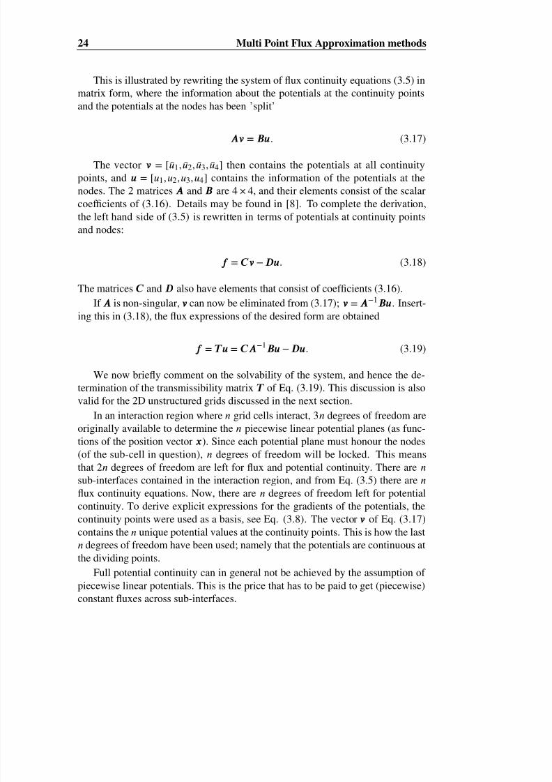
This is illustrated by rewriting the system of ux continuity equations (3.5) inmatrix form, where the information about the potentials at the continuity pointsand the potentials at the nodes has been ’split’
Av = Bu . (3.17)
The vector v = [u1, u2, u3, u4] then contains the potentials at all continuitypoints, and u = [u1, u2 ,u3, u4] contains the information of the potentials at thenodes. The 2 matrices A and B are 4 × 4, and their elements consist of the scalarcoefcients of (3.16). Details may be found in [8]. To complete the derivation,the left hand side of (3.5) is rewritten in terms of potentials at continuity pointsand nodes:
f = Cv − Du . (3.18)
The matrices C and D also have elements that consist of coefcients (3.16).If A is non-singular, v can now be eliminated from (3.17); v = A − 1Bu . Insert-
ing this in (3.18), the ux expressions of the desired form are obtained
f = T u = CA − 1Bu − Du . (3.19)
We now briey comment on the solvability of the system, and hence the de-termination of the transmissibility matrix T of Eq. (3.19). This discussion is alsovalid for the 2D unstructured grids discussed in the next section.
In an interaction region where n grid cells interact, 3 n degrees of freedom areoriginally available to determine the n piecewise linear potential planes (as func-tions of the position vector x ). Since each potential plane must honour the nodes(of the sub-cell in question), n degrees of freedom will be locked. This meansthat 2 n degrees of freedom are left for ux and potential continuity. There are nsub-interfaces contained in the interaction region, and from Eq. (3.5) there are nux continuity equations. Now, there are n degrees of freedom left for potentialcontinuity. To derive explicit expressions for the gradients of the potentials, thecontinuity points were used as a basis, see Eq. (3.8). The vector v of Eq. (3.17)contains the n unique potential values at the continuity points. This is how the last
n degrees of freedom have been used; namely that the potentials are continuous atthe dividing points.Full potential continuity can in general not be achieved by the assumption of
piecewise linear potentials. This is the price that has to be paid to get (piecewise)constant uxes across sub-interfaces.

8/10/2019 Thesis Reservoir Simulation
http://slidepdf.com/reader/full/thesis-reservoir-simulation 37/87
3.2 Unstructured grids; 2D polygonal CVs 25
3.2 Unstructured grids; 2D polygonal CVs
A discussion of the transmissibility calculation for the sub-interfaces of triangularinteraction regions will now be given. In Paper A, the MPFA O-method is dis-cussed for polygonal control volumes, and it is the transmissibility calculationsthat apply for this geometry that will be discussed.
E
Figure 3.7: Left: Polygonal control volume grid with associated triangular interac-tion regions. Right: Whole cell edge, E , covered by two neighbouring triangularinteraction regions.
The geometry may be illustrated by Fig. 3.7, and the notation used for thisgeometry will be the same as in [3], [4] and in Paper A.
The interaction regions of the polygonal control volumes discussed in PaperA, will be triangles. Such an interaction region was visualised in Fig. 3.3. Forthis case, uxes across sub-interfaces will also be given by the general formula(3.1). Now 3 grid cells will interact, so that n = 3 in Eq. (3.1). Further, 3 uxcontinuity equations of the form (3.5) must hold. Similar coefcients as (3.16)were introduced in [3], but the notation is slightly different. More specically, thescalar coefcients for the case of polygonal control volumes are given by
ω ±ik
=n T
i K k ν ±k2F k
. (3.20)
The quantities used in the above coefcients are explained by Fig. 3.8.Note that parts of the triangle edges are used in the denition of the scalar
coefcients (3.20). In Paper A, the continuity points/dividing points of the tri-angle edges are midpoints of the triangular edges, such that the outward normalvectors ν +i and ν − p(i) are equal. However, as the method was derived for arbitrary
continuity points along the triangle edges, we have kept the original notation.The transmissibilities for the sub-interfaces of this triangular interaction re-
gion are derived using exactly the same principles as for quadrilateral controlvolumes. Flux continuity is posed across the sub-interfaces, and potential continu-ity is posed at dividing points. As for the quadrilateral case, explicit expressions

8/10/2019 Thesis Reservoir Simulation
http://slidepdf.com/reader/full/thesis-reservoir-simulation 38/87
26 Multi Point Flux Approximation methods
ν −1
ν +1 ν −2
ν +2
ν −3
ν +3
n 1
n 2
n 3
Figure 3.8: Triangular interaction region with quantities used in scalar coef-cients.
are obtained for the gradients of the potentials for each sub-cell in the interactionregion. For each sub-cell, the potentials at the node and the dividing points areused as a basis for expressing the gradient. This is illustrated by Fig. 3.9, whichshows the corresponding picture to Fig. 3.6, where inward normal vectors of theinteraction region were used for expressing the gradients of the potentials.
ν
ν
x x
k
m(k)
k k −
x−
m(k)
Figure 3.9: Variational triangle
Using these points and vectors, one obtains the general expression for thegradient of the potential of sub-cell k ,k = 1, ..,3 in a triangular interaction region:
∇U k = − 12F
(ν +k (um(k ) − uk ) + ν −k (uk − uk )), (3.21)
where m(k ) is a backward integer function dened by
m(k ) =k − 1, for k > 1,3, for k = 1.
(3.22)
The ux continuity conditions are with this notation stated by

8/10/2019 Thesis Reservoir Simulation
http://slidepdf.com/reader/full/thesis-reservoir-simulation 39/87
3.2 Unstructured grids; 2D polygonal CVs 27
f i,i = f i, p(i) , i = 1, .., 3. (3.23)
The indexing p(i) denotes the forward integer function
p(i) =i + 1, for i < 3,3, for i = 3.
(3.24)
When inserting the scalar coefcients in Eq. (3.23) and the ux expressionf i = − n T
i K j∇U j for sub-interface i, one obtains a similar system of equations asEq. (3.17). In the original paper [3], the system of ux continuity equations waswritten as
Av + Bu = Cv + Du . (3.25)
As in the discussion of the transmissibility calculations for the case of quadri-lateral grids, v denotes pressure values at the continuity points, and u denotes thepressures at the nodes of the cells that interact.
The above system of equations is written differently from the system (3.17)by the fact that the information there was split, so that matrices acting on v andu respectively were dened. This is purely an issue of denition. The matrixdifference ( A − C ) of Eq. (3.25) serves as the matrix A of system (3.17), and thematrix difference ( D − B ) of (3.25) serves as the matrix B of system (3.17).
The matrices A, B , C and D of the system of equations (3.25) are dened,and can be found on p.6 of Paper A. Their elements consist of scalar coefcients(3.20). As in the discussion of the transmissibility calculations for the quadri-
lateral case, the potentials at the continuity points may be eliminated. From Eq.(3.17) one obtains
v = (A − C )− 1 (D − B )u . (3.26)
Together with, for example, the left hand side expression for the ux of (3.17),the transmissibilities are found:
f = A (A − C )− 1(D − B )u + Bu . (3.27)
Hence, the transmissibility matrix is
T = A (A − C )− 1 (D − B ) + B . (3.28)
Having found the transmissibilities, the coefcient matrix for the total systemof discrete pressure equations may be found by an assembly procedure. This isalso discussed in Paper A.

8/10/2019 Thesis Reservoir Simulation
http://slidepdf.com/reader/full/thesis-reservoir-simulation 40/87
28 Multi Point Flux Approximation methods
3.3 Faults with crossing grid lines
3D structured grids are the most commonly used grids for eld reservoir simula-tion. This is mostly because of the frontier commercial simulator Eclipse [57],where structured, orthogonal, conforming quadrilaterals were used in the rst re-leased versions. Although the grids are structured, one is faced with several chal-lenges if for instance faults need to be taken into account. Grid cells need nolonger be conforming, and the discretisation of uxes across cell edges must bere-investigated.
Paper C of Part II extends the MPFA methods to handle cases where lateralgrid lines are allowed to intersect. Examples of such grids are encountered whenusing (Geophysical) models for real elds. In particular, the North Sea reservoirVisund uses a reservoir description where such faults are found. The simulatorEclipse allows reservoir simulation for this grid type, but the ux discretisationuses a standard two-point ux expression, see [6] and [57] for details.
MPFA Transmissibility calculations to handle faults with crossing lateral gridlines are presented in Paper C, and the discretisation uses the same principles asfor previously investigated grid types. Note, however, that some additional issuesneed to be taken care of because of the under-determined character the system of equations that determines the transmissibilities has.
Before discussing these special 3D faults, we briey discuss standard faults in2D and 3D. The extension of the MPFA method to handle faults was rst done for2D quadrilateral grids in [6]. Here the concept of non-conforming grids was used,and interaction regions were dened around such corners. As seen in Fig. 3.10,three grid cells meet in a corner.
Fault line
Figure 3.10: Corners when faults are encountered in 2D
A natural interaction region to use here is the triangular interaction regionwhich was introduced in Sec. 3.2, or a similar interaction region where three gridcells interact. It has been reported that this interaction region has an apparent dis-advantage when one of the grid cells of the interaction region is inactive [6], whereit was shown that there will be no ow across one of the three sub-interfaces for

8/10/2019 Thesis Reservoir Simulation
http://slidepdf.com/reader/full/thesis-reservoir-simulation 41/87
3.3 Faults with crossing grid lines 29
certain situations. Instead, in [6] it was suggested to use an extended interaction
.
.
.
.
.
.
.
.
.
.
1 2
3 4
5
Figure 3.11: Interaction region associated with 2D faulted corners. Five grid cellsinteract
among grid cells. The suggested interaction region will contain information from5 grid cells instead of 3. Hence, the uxes across each of the sub-interfaces i are
expressed as
f i =5
j = 1
t ij u j . (3.29)
This is visualised in Fig. 3.11. The MPFA method was extended to faultedcorners in 3D in [7]. Similar ideas as for the 2D faults were used to derive trans-missibilities for the extended interaction regions, and details may be found in [7].Five different situations may occur, and the ux molecules will contain informa-tion from 8 to 11 grid cells. One possible situation is illustrated in Fig. 3.12, where7 grid cells meet in a corner. For this case the ux molecules contain information
from 9 grid cells. These types of corners will be termed regular corners , and 5-8
Figure 3.12: Ordinary faulted corners in 3D
grid cells will touch upon such corners. However, in [7] the case where grid linesintersect was not discussed. This situation was discussed in Paper C. Lateral gridlines may for some simulation grids cross, and the ux across general polygonalux interfaces must be discretised. The point for which lateral grid lines intersect,will be termed an irregular corner , and an interaction region will be associated

8/10/2019 Thesis Reservoir Simulation
http://slidepdf.com/reader/full/thesis-reservoir-simulation 42/87
30 Multi Point Flux Approximation methods
with it. How these new corners arise is depicted in Fig. 3.13. For this corner, 4grid cells will touch upon it, and these 4 grid cells will be the interacting grid cellsin the associated interaction region. The sub-interfaces for which the transmiss-ibilities need to be calculated are visualised in Fig. 3.14. Here, 6 sub-interfaces
will be associated with the interaction region. To understand this, consider Fig.3.13. The local numbering of the four grid cells is as follows: Local grid cell1 is the front cell, grid cell 2 is the back cell. Above cell 1 there will be a gridcell (not drawn), and this cell has local number 3. Above cell 2, grid cell 4 willbe located (also not drawn). A cell interface is a a sharing of a common surfacebetween two neighbouring grid cells. From Fig. 3.13 it is seen that there will be6 cell interfaces touching upon the irregular corner. Denoting these sharings bya tuple ( a 1, a 2) (where a1 and a2 correspond to the local numbering of the gridcells), the 6 sharings are given by (1,3), (2,4), (1,2), (1,4), (3,2) and (3,4). The6 sub-interfaces will be parts of these 6 cell interfaces, and this is discussed below.
For each of the 6 sub-interfaces we want to nd uxes that are linear combin-ations of these 4 interacting grid cells:
f i =4
j = 1
t ij u j , i = 1, ..., 6. (3.30)
1
2
3
4
Figure 3.13: Crossing grid lines arising from faults
As for the 2D case, ∇U is needed in order to derive discrete uxes and trans-
missibilities for the sub-interfaces belonging to this new type of interaction region.This is done by using the same methodology as in [8]. For three-dimensionalcases (ie. both this situation and the situation with ordinary faulted corners), ∇U for each sub-cell of an interaction region, can be dened implicitly by the valuesof the potentials at three corresponding potential continuity points:

8/10/2019 Thesis Reservoir Simulation
http://slidepdf.com/reader/full/thesis-reservoir-simulation 43/87
3.3 Faults with crossing grid lines 31
2
3
4
56
1
Figure 3.14: Sub-interfaces associated with irregular corner
X ∇U =u1 − u0u2 − u0u3 − u0
. (3.31)
The derivation of the inverse of X follows exactly the same ideas as for the
2 dimensional case. We introduce variational tetrahedra spanned by the cellcentre x0 (node) and three local continuity points x 1, x 2 , x 3 that are located onthe three sub-interfaces seen from the sub-cell in question. These points are loc-ally numbered cyclically. A variational tetrahedron used for the faulted corners in3D discussed in [7] is visualised in the left hand side of Fig. 3.15. The continuitypoints are three of the corners of the tetrahedron, and are located on 3 separatesurfaces of the cell in question. Due to the special geometry when lateral gridlines are allowed to intersect, the variational tetrahedra will be somewhat differ-ent from the regular case. This is depicted in the right hand side of Fig. 3.15. Twoof the tetrahedron corners will be located on the same cell interface (claried byFig. 3.17).
4 of the 6 sub-interfaces are parts of side surfaces of the grid cells that interact,whereas the two remaining sub-interfaces are parts of the top/bottom surfaces of the cells of the interaction region. This is visualised in Fig. 3.14. The 4 sub-interfaces that lie in the surface generated by the side surfaces of the grid cellsthat interact are numbered 3-6 in the gure. In Paper C it was assumed that theside surfaces of the cells are planar, and the surfaces 3-6 will hence also be planar.
To better see how these four sub-interfaces arise, it may be useful to visualisethe situation orthogonally on the intersection, as in Fig. 3.16.
Different situations may occur, and the whole cell interfaces that touch uponthe corner may have from 3 to 6 corners. Each of these corners will correspond
to an interaction region. For a complete discretisation of the uxes across thewhole cell interfaces, the cell interface will be shared among the 3-6 interactionregions which the corners of the whole ux interfaces correspond to. The sharingof ux-interfaces among the interaction regions may easily be dened by dividinga whole cell interface with n corners into n segments/sub-interfaces. This is done

8/10/2019 Thesis Reservoir Simulation
http://slidepdf.com/reader/full/thesis-reservoir-simulation 44/87
32 Multi Point Flux Approximation methods
x
x
x
x x
x
1
2
3
1
3
2
Figure 3.15: Variational tetrahedra for a) regular case b) crossing grid lines.
Front
Back
Figure 3.16: Intersection of lateral grid lines seen orthogonally on the intersection
by nding the geometric centre of the cell interface ( x = 1/ n x i), and drawingstraight lines to the midpoint of all edges. All sub-interfaces will then have 4edges, and the approach is easy to implement.
34
5
6
Figure 3.17: Sub-interfaces belonging to side surfaces of grid cells
Fig. 3.17 explains how sub-interfaces 3-6 of Fig. 3.14 arise. At each sub-interface there will be one point for which the potentials of neighbouring grid cellsare continuous, ie. a continuity point. These points are marked with dots, andtheir numbering corresponds to the numbering of sub-interfaces. This explains

8/10/2019 Thesis Reservoir Simulation
http://slidepdf.com/reader/full/thesis-reservoir-simulation 45/87
3.3 Faults with crossing grid lines 33
why two of the corners of the variational tetrahedra used here are located on thesame side surface (of the cell in question).
For all 6 sub-interfaces, ux continuity will be posed, and (together with po-tential continuity at 6 points) this leads to a local system of equations to determine
the transmissibilities of the interfaces. This system is written out in Paper C, andthe redundancy of the system is discussed. The redundancy implies that moreconditions are needed in order to determine the transmissibilities. The determina-tion of transmissibilities for the sub-interfaces was partially answered by using acriterium for no-ow and a criterium for uniform ow in Paper C. Details may befound in the paper.
Linear ow assumes a homogeneous medium, and it is not clear whether thetransmissibility calculations can be generalised to arbitrary heterogeneous mediawithout additional information.

8/10/2019 Thesis Reservoir Simulation
http://slidepdf.com/reader/full/thesis-reservoir-simulation 46/87
34 Multi Point Flux Approximation methods
Figure 3.18: Gridding of region of interest; inner grid cells are sketched by con-tinuous lines. Grid cells surrounding the area of interest are indicated by dottedlines.
3.4 Treatment of Dirichlet boundary conditions
The rst published papers on MPFA methods [1]-[8] handled boundaries withhomogeneous Neumann conditions. The implementation of such conditions werestraight forward since the transmissibility coefcients could be calculated by thesame ideas as for the fully active interaction region. Details may be found in [3].
Paper D investigates convergence of the O-method on some quadrilateral gridsin 2D. Such a study requires more general conditions than homogeneous Neu-mann conditions. All our analytical examples required using xed potentials atsome boundary.
We now discuss various ways of how to extend the MPFA O-method for 2Dquadrilateral grids to account for general Dirichlet conditions.
The simplest way to include xed potentials at boundaries is to add an en-circling layer of articial grid cells around the medium which we study. If theanalytical pressure solution is known, we may x the potentials at these outercells, and solve the discrete pressure equations for all the inner grid cells (at thenodes). At each renement level one solves the pressure equation on the samephysical medium, as illustrated by Fig. 3.18.
This approach does not incorporate the boundary conditions (Dirichlet andNeumann) for the ’active area’ exactly, but rather approximately. This can beseen in Figure 3.19, where an extended interaction region is shown. The pointsx 3a and x 4a are nodes of the articial grid cells, and at these points we use exactpressures. The transmissibility calculations then yield approximate uxes f 1d and
f 2d and corresponding discrete pressures at the continuity points x 2d and x 4d .As the approach above requires that the analytical solution is known outside
the area of interest, a better approach of handling general Dirichlet boundary con-ditions is to actually incorporate xed potentials/pressures at the actual boundariesof the medium we study. Utilising the ideas from the original transmissibility de-

8/10/2019 Thesis Reservoir Simulation
http://slidepdf.com/reader/full/thesis-reservoir-simulation 47/87
3.4 Treatment of Dirichlet boundary conditions 35
x x
x x
f f x x
1 2
x x1d 2d
− − 4d 2d
3a 4a
Figure 3.19: Incorporation of approximated boundary conditions
x x
x
x
x
1 2
2D1D
F
Figure 3.20: Treatment of Dirichlet boundary conditions
rivations, this can be done by studying an interaction region which covers a partof the boundary.
Consider the extracted part of a grid visualised in Fig. 3.20. The nodes of thetwo grid cells are x1 and x 2 respectively. The points x D 1 and x D 2 are points onthe boundary, and the potentials at these point will be specied by the Dirichletboundary conditions. To derive the transmissibilities for the sub-interface goingfrom x F to the boundary, we pose continuity of the ux at the sub-interface andcontinuity of potential at the dividing point x F . When the potential is assumedto be piecewise linear in each of the sub-cells for the cells that interact in theinteraction region, the local system is closed with respect to degrees of freedom.
Hence, we may derive the transmissibilities through the equation
− K 1∇U 1 · n = − K 2∇U 2 · n . (3.32)
The gradients can be calculated by using variational triangles dened on eachsub-cell and the notation used in Sec. 3.1. Hence,
∇U i = 1T iν ik (uik − ui ), (3.33)
for the each of the cells i = 1,2. The vectors ν ik are as before the inward normalvectors of the edges ( x ij − x i) of the variational triangles ( j , k cyclic, k local num-bering of dividing points of triangle). T i is equal to twice the area of variational

8/10/2019 Thesis Reservoir Simulation
http://slidepdf.com/reader/full/thesis-reservoir-simulation 48/87
36 Multi Point Flux Approximation methods
triangle i. The potentials uik are the potentials at the points x ik (ie. either potentialat boundary or at continuity point x F ).Having expressed the gradients, the ux continuity equation (3.33) now reads
− 1T 1 K 1(ν 11 (u1D − u1) + ν 12 (uF − u1))n =
− 1T 2
K 2(ν 21 (uF − u2) + ν 22(u2D − u2))n . (3.34)
This may be written as
av = bu + k 1u , (3.35)
where a (scalar), b and k 1 (1x2 vectors) depend on geometry and permeability.Further, v = uF is the unknown potential at the dividing/continuity point x F , u =
[u1, u2] represents the vector of node potentials, and u = [u1D , u2D ] is the vectorinvolving the pressures u1D and u2D specied by the boundary conditions.
The entities a , b and k 1 of Eq. (3.35) can be given explicitly:
a = − 1T 1
K 1ν 12n +1
T 2K 2ν 21n
b = [− 1T 1
K 1(ν 11 + ν 12)n , 1T 2
K 2(ν 21 + ν 22)n ]
k 1 = [ 1T 1
K 1ν 11 n , − 1T 2
K 2ν 22n ] (3.36)
To express the transmissibilities for the sub-interface, we may write the left handside of (3.34) as
f = cv − du + k 2u1D , (3.37)
where c (scalar), d (1x2 vector) and k2 (scalar) depend on geometry and permeab-ility. These can also be given explicitly:
c = 1T 1
K 1ν 11n
d=
[− 1T 1 K 1(ν 11
+ν 12)n ,0]
k 2 = − 1T 1
K 1ν 11 n (3.38)
The unknown uF may now be eliminated from Eq. (3.35):

8/10/2019 Thesis Reservoir Simulation
http://slidepdf.com/reader/full/thesis-reservoir-simulation 49/87
3.4 Treatment of Dirichlet boundary conditions 37
x x
x
e
ee1D 2D1D
1
2D
1F
x
x
2
Figure 3.21: Boundary interaction region, used to include Dirichlet boundary con-ditions.
v = a − 1(bu + k 1u ), (3.39)
and inserting this in Eq. (3.37) yields
f = (ca − 1b − d )u + ca − 1k 1u + k 2u1D . (3.40)
Hence, the ux is expressed as
f = T u + T u . (3.41)
The transmissibilities from T will enter the system matrix A for the discreteset of (pressure) equations MU = R , and the transmissibilities from T will enterthe right hand side R of the system. To construct the full system matrix, a loopingover all interaction regions will be done, and for inner interaction regions wecalculate transmissibilities in the standard way, discussed in Sec. 3.1.
The above method to take Dirichlet boundary conditions into account seemto be a reasonable way to handle the problem. However, for K -orthogonal grids,some information seems to be lost from the boundary because of the orthogonalityof the grid. Moreover, the elements of T of Eq. 3.41 will be zero for the casedepicted in Fig. 3.22. It is possible to move the continuity point and the boundarypoints x 1D and x 2D in such a way that the same points as in Edwards’ [17] MPFAmethod are obtained. When this is done, the elements of T in (3.41) will ingeneral be nonzero.
The third way to deal with Dirichlet boundary conditions for the MPFAmethod is to somehow include uxes on the boundary as well.The information about the pressure on the boundary will as before be included
for the transmissibility calculations, as illustrated in gure 3.21. The potentialvalues at the boundary are used in the expressions for the gradient of potentials

8/10/2019 Thesis Reservoir Simulation
http://slidepdf.com/reader/full/thesis-reservoir-simulation 50/87
38 Multi Point Flux Approximation methods
K
K y
x
Figure 3.22: K -orthogonal grid; ’Dirichlet’ transmissibilities will be zero
for each cell. From this, the discrete uxes for the sub-interfaces are
f 11 = − K 1∇U 1 · n e1 (3.42)f 12 = − K 2∇U 2 · n e1 (3.43)
f 1D
= − K 1∇U
1· n
e1D (3.44)
f 2D = − K 2∇U 2 · n e2D (3.45)
The gradient, ∇U i , i = 1,2 will use the potential values at the points x i , x Di andx F . The ux from cell 1 into the ux interface e1 , calculated by the informationfrom cell 1, is denoted f 11 , and equals the ux calculated for interface e1 into cell2, (information from cell 2), f 12 . The potential at the dividing point x F may hencebe eliminated, from Eq. (3.42) and Eq. (3.43). If we next use the potential at thedividing point x F in (3.43)-(3.45), we are left with the ux f = (f 12 , f 1D , f 2D )T asa function of the potentials of the active cells 1 and 2, u = (u1 , u2)T , and potentialsat the boundary, u = (u(x D 1), u(x D 2))T .
The uxes can now be expressed as:
f = T u + T u
The transmissibilities of T will be incorporated in the the discrete version of (2.1), while T u incorporates the boundary conditions on the right hand side of the corresponding discrete system.

8/10/2019 Thesis Reservoir Simulation
http://slidepdf.com/reader/full/thesis-reservoir-simulation 51/87
Chapter 4
Time dependent problems
Reservoir simulation models are used to predict future performance of reservoirs.For multiphase problems the ow is hardly ever stationary, so in order to make
forward simulations (in time), the time dependent terms of the governing PDEsmust also be discretised.Several options are possible, but it is common to use backward Euler time
discretisation to obtain fully implicit discrete equations. This means that all un-knowns are coupled at a given time level, and the equations for the unknowns needto be solved simultaneously. A semi discrete version of the mass balance equationfor phase α then reads
mnα − mn− 1
α + ∆ tn
j
f nαj = q nα . (4.1)
The entities above are: mα accumulated mass of phase α , n and n − 1 time levels,f αj phase uxes through surface number j of a control volume, and q α a possiblesource term. Nonlinearities and how these affect the numerical solution strategyare discussed next.
4.1 Nonlinearities
The discretisation of multiphase ow equations/problems yields sets of non-linearequations to solve (with respect to solution variables). The non-linearities arisebecause of the appearance of relative mobilities (see Chapter 1) of the phase uxes
kri
µ i K ∇ ui · n , and the inclusion of capillary pressure. Relative mobilities will behandled by standard upstream evaluation across edges. A possible modicationof this has not been an issue for the MPFA O-method yet. This means that thethe transmissibilities derived for single phase ow will be scaled by relative mo-bilities according to the ow direction. By an implicit solution strategy, relative

8/10/2019 Thesis Reservoir Simulation
http://slidepdf.com/reader/full/thesis-reservoir-simulation 52/87
40 Time dependent problems
permeabilities will be updated at each iteration level.At each time level, indicated by Eq. (4.1), nonlinear algebraic equations must
be solved. Our in-house research simulator solves these algebraic equations byusing a Newton discretisation approach, see for instance [39], [40].
Based on the time stepping, an outer iteration is dened, and the goal is tosolve the equation based on Eq. (4.1), which determines the change in solutionvariables from one time step to the next time step
r (x ) = m(x ) − mn − ∆ tk
f k (x ) − ∆ tq (x ) = 0. (4.2)
Here x denotes the vector of the (primary) solution variables in all grid cells.For three-phase ow these may be the three quantities po, S w and S g , and theremaining 3 solution variables ( S o, pw , pg ) are found by the previously discussedclosure relations.
The solution by the Newton discretisation procedure is dened by
(∂r∂x
)ν − 1[x (ν ) − x (ν − 1) ] = − r (ν − 1) , (4.3)
where the superscripts ν and ν − 1 denote iteration levels. Eq. (4.3) is solveduntil x (ν ) − x (ν − 1) has reached some desired limit (ie. specied convergence cri-teria). The data structure of the research simulator allows for general geometry,and this will be reected in the Jacobi matrix ( ∂r
∂x ). Moreover, there will be morecouplings in the Jacobi matrix when a control volume interacts with more controlvolumes than when two point ux schemes are used for ux discretisation. Thisgeneralisation is accounted for in, for example, the handling of simulation gridswith crossing lateral grid lines in Paper D. Details of the Newton strategy may befound in [39].

8/10/2019 Thesis Reservoir Simulation
http://slidepdf.com/reader/full/thesis-reservoir-simulation 53/87
Chapter 5
Numerical results
Paper D investigates convergence numerically for the MPFA O-method. In the lit-erature, there are numerous reference examples to be found for the purely elliptic
problem (1.7) with suitable boundary conditions. Linear pressure solutions (inspace) are perhaps the easiest reference solutions to investigate. Although sucha reference solution is very simple, it is a good rst test to examine the discretesolution obtained by a discretisation method when the grid is challenging.
The discrete ux operator is examined for various non-orthogonal grids inboth 2D and 3D in Paper D. It is shown that the discrete uxes (from the MPFAO-method) across sub-interfaces of interaction regions are exact when applied tolinear potentials. Intuitively we should expect that the discrete pressure solutionobtained from the corresponding system Au = b also should be exact since thediscrete set of pressure equations is constructed by assembly of transmissibilities.
The pressure solution on a randomly perturbated grid is investigated for theSupport Operator Method (SOM) for a homogeneous medium in [44], where theanalytical ow is uniform in a given direction. Their discrete pressure solution isexact for that case.
Fig 5.1 shows a random 8 × 8 grid, and the underlying medium is homogen-eous. The discrete pressure solution is calculated by the MPFA O-method, wherethe analytical pressure solution is linear (driven by specied (Dirichlet) pressureson the left and right hand side of the medium). The right hand plot of Fig. 5.1reveals that the pointwise pressures are linear and exact for this case.
A similar test can be carried out for a discontinuous coefcient problem, wherethe analytical pressure solution is piecewise linear. The medium is divided into
two parts, and the permeability ratio is 1/10 across the medium discontinuity. Thediscontinuity line is here given by rx + sy = 0, where r = tan (π /3)/(1 + tan (π /3))and s = 1/(1 + tan (π /3)). This is visualised in Fig. 5.2. The permeabilities arek x = k y = 10 for rx + sy < 0 and k x = k y = 1 for rx + sy > 0. The true solution isgiven by

8/10/2019 Thesis Reservoir Simulation
http://slidepdf.com/reader/full/thesis-reservoir-simulation 54/87
42 Numerical results
−0.8 −0.6 −0.4 −0.2 0 0.2 0.4 0.6 0.8−0.8
−0.6
−0.4
−0.2
0
0.2
0.4
0.6
0.8
−0.2 0 0.2 0.4 0.6 0.8 1 1.2−0.2
0
0.2
0.4
0.6
0.8
1
1.2
x−coordinate
P r e s s u r e
a. Random grid;. b. Pressure vs. x-coord
Figure 5.1: Numerical pressure solution; uniform ow in x -direction.
−0.5 −0.4 −0.3 −0.2 −0.1 0 0.1 0.2 0.3 0.4 0.5−0.5
−0.4
−0.3
−0.2
−0.1
0
0.1
0.2
0.3
0.4
0.5
−0.5 −0.4 −0.3 −0.2 −0.1 0 0.1 0.2 0.3 0.4 0.5−0.5
0
0.5
−1
0
1
2
3
4
5
a. Random grid. b. Discrete pressure solution
Figure 5.2: Numerical pressure solution; discontinuous coefcient problem.Piecewise linear reference solution.
u(x , y ) =rx + sy , for rx + sy < 0,10( rx + sy ), for rx + sy > 0.
(5.1)
The numerical results are shown in Fig. 5.2, where the pressures at the grid nodesare employed. The discrete pressure solution on our 16 × 16 grid is piecewise
linear and exact also for this case.More sophisticated cases are tested in Paper D. Especially interesting test
cases are cases where the permeability of the medium has sharp jumps, and theanalytical solution exhibits singularities in the velocity eld. Such reference solu-tions are discussed in [46].

8/10/2019 Thesis Reservoir Simulation
http://slidepdf.com/reader/full/thesis-reservoir-simulation 55/87
5.1 Analytical solutions 43
−0.5
0
0.5
−0.5
0
0.5−10
−5
0
5
10
Figure 5.3: Plot of analytical solution on [ − 0.5,0.5] × [− 0.5,0.5]. Solution exhib-its singularity at the origin.
5.1 Analytical solutions
The problems dealt with in Paper D are special cases where analytical solutionsof the elliptic equation (1.7) are known. The cases are discussed because theyregard important physics which discretisation methods should handle. In reservoirsimulation, non-orthogonal grids are used extensively, and the permeabilities varyfrom grid cell to grid cell. Four grid cells will meet at each corner for a conforminggrid. If the grid cells have different permeability, the pressure may be less regularnear these corners than in areas where the medium is homogeneous.
In particular, cases where the analytical solutions exhibit singularities, shouldbe discussed. Such a solution is depicted in Fig. 5.3 on a square domain. Usingpolar coordinates, this is a solution of the form
ui (r , θ ) = r β (acos (βθ ) + bsin (βθ )), (5.2)
where the index i denotes regions with different permeability. The parameter β denes the regularity of the solution, and will depend on heterogeneity and theangles of the grid cells that meet at a corner. These functions are known to notbelong to the function space H 2(Ω ), but rather the fractional space H 1+ ν (Ω ),where ν < β , see [46]. The solutions are derived based on separation of variables,and details may be found in Strang and Fix [46].

8/10/2019 Thesis Reservoir Simulation
http://slidepdf.com/reader/full/thesis-reservoir-simulation 56/87
8/10/2019 Thesis Reservoir Simulation
http://slidepdf.com/reader/full/thesis-reservoir-simulation 57/87
Chapter 6
Properties of discrete system
There has recently been work done to investigate the relationships between MFE-types of methods and MPFA methods, [30] and [32]. Furthermore, these relations
are used to analyse convergence of the MPFA O-method on a general quadrilateralgrid (with continuously varying heterogeneity) theoretically [32].As the MPFA method does not directly build on a variational formulation of
the governing (elliptic) equation, the approach in Paper A was not to investig-ate convergence but rather to investigate the coefcient matrix that arises whendiscretising Eq. 2.1. This matrix is also frequently referred to as the Discreteoperator (corresponding to the continuous operator).
Various works in the literature, [41], [42] etc., indicate that convergence of adiscretisation method is related to three important issues; conservation of mass,consistency of uxes (see discussion in [4]) and stability. MPFA-methods arelocally mass conservative, so this is not an issue to be discussed. The concept of consistent ux means that the discrete uxes are ’reasonably’ approximated. Weclaim that this is the case for uxes obtained by the MPFA approach, since theseallow for general geometry, and general tensor representation of permeabilities.Exceptions are cases where the solutions are far from H 2-regular, as indicated bythe last numerical example of Paper D.
Stability issues are among the reasons for studying the discrete operator. Cer-tain important properties of the continuous elliptic operator should be inherited forthe discrete operator. The operator ∇ · (K ∇ ) is a self adjoint operator, and thediscrete operator should then ideally be symmetric [43]. This was one of the issuesdiscussed in Paper A (see discussion of Paper A below). Stability of a method is
assured if the discrete system satises the coercivity condition [8], [51]:uT Au ≥ µuT Du , (6.1)
where A denotes the coefcient matrix of the system, and u denotes the discretesolution vector. For the coercivity condition to be satised, A should be positive

8/10/2019 Thesis Reservoir Simulation
http://slidepdf.com/reader/full/thesis-reservoir-simulation 58/87
46 Properties of discrete system
denite [49].A special class of matrices that are positive denite, are symmetric M-matrices:
6.1 M-matricesThe following denition is taken from [51].
Denition : A matrix A is called an M-matrix if the following is satised:
a) The diagonal elements a ii are positive whereas the off-diagonal termsa ij , i = j are non-positive.
b) A is non-singular and A − 1 ≥ 0.
Such matrices are appealing when looking at the continuous problem−∇ · (K ∇ u) = q . For positive sources q , the solution u should also be pos-itive, and this is assured if the coefcient matrix that arises from the discretisationof −∇ · (K ∇ ) is an M-matrix. Moreover, the positiveness of the solution isassured if the coefcient matrix has a non-negative inverse. Such matrices arecalled monotone (operators), see also [8] for a discussion.
The M-matrix property is examined in Paper A. However, this property maybe too restrictive for a method in order to say something about the monotonicity.It is well known that a matrix may have a non-negative inverse without being anM-matrix. This means that the matrices one really is looking for, are matricesthat are symmetric, positive denite, and have non-negative inverses. As far as weknow, it is not known how such matrices can be classied based on their elements,but work has been done recently to analyse the monotonicity of the O-method.
6.2 Notes on violation of maximum principle
A specic case has been investigated in [15] where it was of interest to nd outwhether a non-negative inverse still could be obtained even though the conditionsfor the matrix to be an M-matrix were violized. The O-method was examined on aparallelogram grid (2D) for homogeneous media. The coefcient matrix will then
be described by the legs of the grid cells (and the corresponding inner angles of the grid cells). The elements of the coefcient matrix are given by the cell stencilfor the central cell (cell 1) of Fig. 6.1. These coefcients are denoted m1.....m9,and correspond to the local numbering of grid cells in Fig. 6.1. For the O-methodon a parallelogram grid on a homogeneous medium, these coefcients are given

8/10/2019 Thesis Reservoir Simulation
http://slidepdf.com/reader/full/thesis-reservoir-simulation 59/87
6.2 Notes on violation of maximum principle 47
by [8]
1 2
345
6
7 8 9
Figure 6.1: Local numbering of grid cells
a = a 1T K a 1, b = a 2
T K a 2, c = a 1T K a 2, (6.2)
and
m2 = − a +c2
d, m3 = −
c2
− c2
2d, m4 = − b +
c2
d, m5 =
c2
− c2
2d, (6.3)
and mi+ 4 = mi , i = 2, ...,5. The variable d is given by 2 ab /(a + b), and m1 =
− i= 2 9mi . The permeability K is positive denite such that a > 0, b > 0, andc2 < ab . It is shown that two criteria are sufcient for the coefcient matrix A tohave a non-negative inverse. These criteria are
(1) m2 · m4 − m3 · m1 ≥ 0, (2) m2 · m4 − m5 · m1 ≥ 0, (6.4)
which are the same as |c| (2 − c2ab ) ≤ d . Since these criteria only are sufcient, the
inverse will be non-negative even if (6.4) is not satised. In [15] it is stated that forgrids with approximately unity aspect ratios, grid skewness of about 45 degreesmay be allowed. For stronger aspect ratios and/or anisotropy ratios, the limitationson grid skewness are more severe. The reader may notice that grid skewness of 45 degrees has been tested in Paper D for various reference solutions.
When the inverse is investigated numerically on an n × n grid, it is found thatangles down to π /6 yield positive inverses for large n (n approximately 20) foraspect ratios in the interval (1/2,2).
This result may be interpreted as an unfortunate way of choosing neighbouring
information for the uxes across cell edges when the grid cells are very skewed.When the aspect ratio of the grid is close to 1, it is possible to construct a schemewhere the bandwidth is reduced. This should intuitively lead to a more diagonallydominant matrix than the 9-point scheme does. Such a scheme can be illustratedby Fig. 6.2.

8/10/2019 Thesis Reservoir Simulation
http://slidepdf.com/reader/full/thesis-reservoir-simulation 60/87
48 Properties of discrete system
23
4
1
Figure 6.2: Possible 7-point cell molecule. Combination of different types of interaction regions
This molecule can be obtained by combining two types of interaction regions.Interaction region 2 and 4 are triangular interaction regions which are special casesof the triangles investigated in Paper A. Interaction region 1 and 3 are standard in-teraction regions associated with (conforming) corners for 2D quadrilaterals. Thisscheme has not been implemented by us, but for the homogeneous case the schememay easily be generated by the use of explicit expressions for transmissibilities of sub-interfaces of the two different types of interaction regions.

8/10/2019 Thesis Reservoir Simulation
http://slidepdf.com/reader/full/thesis-reservoir-simulation 61/87
Chapter 7
Summary of the papers
Summaries of the papers which Part II of this thesis consists of, will now be given.Some issues may also have been left out of the papers themselves, and some of
these are discussed here. Details are also to be found in the previous sections.
7.1 Summary of Papers A and B
This Subsection will give an overview of Paper A and Paper B:
Paper A: Symmetry and M-matrix Issues for the O-method on an Unstruc-tured Grid Authors: G.T. Eigestad, I. Aavatsmark, M. Espedal
Paper B: MPFA applied to Irregular grids and Faults .Authors: G.T. Eigestad, I. Aavatsmark, E. Reiso, H. Reme, R. Teigland.
The theme is similar for both papers. The MPFA O-method is discussedfor irregular 2D grids in Paper A, and an extension to account for certain griddingsituations which arise when faults occur in 2D, is discussed in Paper B.
Paper A discusses the O-method for polygonal control volumes. These willbe control volumes for which the interaction regions are triangles. The MPFA O-method for such cases is also referred to as the Triangle method in the literature.
It is of interest to study the coefcient matrix that arises when the elliptic
term −∇ (K ∇ u) is discretised. Because the underlying continuous operator isself-adjoint , this should ideally be inherited for a corresponding discrete operator(coefcient matrix). This means that the matrix should be symmetric and positivedenite (since K is positive denite). There exist alternative discretisation meth-ods (Support Operator Methods, [43]), which actually use the preservation of such

8/10/2019 Thesis Reservoir Simulation
http://slidepdf.com/reader/full/thesis-reservoir-simulation 62/87
50 Summary of the papers
properties for the construction of discrete schemes. Secondly, the physics behindthe purely elliptic problem (2.1) implies that positive sources q should lead topositive pressures (for homogeneous Dirichlet boundary conditions). Translatedto the discrete problem, this means that the coefcient matrix should be monotone,
see Chapter 6 and [8].The interaction regions are as mentioned above triangular, and three grid cellsinteract in such an interaction region. This was visualised in Fig. 3.8. The deriva-tion of the transmissibilities are discussed in Sec. 3.2.
The rst case studied in the paper is the case with homogeneous permeability(for the whole medium). For this case, the coefcient matrix is shown to be sym-metric as long as the dividing points (see Sec. 3.2) are midpoints of triangle edges.Further, the dual triangular grid should satisfy the Delauney condition in order forthe coefcient matrix to be an M-matrix. This means that opposite angles of tri-angles which share an edge, should satisfy the condition θ1 + θ2 < π .For general permeabilities, symmetry of the discrete operator is not satised dir-
ectly for the MPFA O-method applied to polygonal control volumes. This wasfurther examined in the paper, and the question raised was whether it is possibleto obtain a symmetric, discrete operator. To answer this question, symmetry equa-tions were dened locally for the interaction regions. The dividing points werexed (midpoints of triangle edges), and the equations were solved with respectto the location of the triangle points inside the interaction regions. The controlvolumes change with this procedure, but the goal of the experiment is to nd geo-metrical situations for which symmetry of the discrete operator is satised. Solu-tions of the symmetry equations may be sought for arbitrary heterogeneity andanisotropy ratios inside the interaction regions. The algorithm for nding trianglepoints that yield symmetric coefcient matrices, may easily be implemented fornumerical purposes. We were not able to obtain solutions for all cases we tested(anisotropic cases), but we were able to extract important information for layeredmedia (two cells of an interaction region have the same permeability). For thesecases it is possible to construct grids a priori that honour the media discontinuities,and at the same time yield coefcient matrices that are symmetric. For isotropiccases it was found that the triangle point should be located on a straight line whichconnects two dividing points, and we refer to Paper A for details. If the anisotropyratios are different, but the principal axes of the permeability tensors are alignedwith the discontinuity line, the triangle point should also be located on this straightline.
This result was found using the symmetry algorithm numerically, and is laterproven analytically in the paper.
The next question raised in the paper is how the dual triangular should bein order for the local contributions from the interaction regions to the coefcientmatrix to have ’the correct’ signs. This is referred to as local M-matrix property

8/10/2019 Thesis Reservoir Simulation
http://slidepdf.com/reader/full/thesis-reservoir-simulation 63/87
7.1 Summary of Papers A and B 51
in the paper. It is found that this local M-matrix property yields a constraint onangles of the dual triangular grid, heterogeneity and anisotropy combined.
The local M-matrix property does not fully answer the question whether thetotal coefcient matrix is an M-matrix, as a neighbouring interaction region may
compensate for unwanted signs/contributions from one interaction region. TheM-matrix property derived for homogeneous media in Paper A is an example of this. Such an analysis may be carried out in the same manner as in Paper A toanswer this for specic cases.Paper B is an overview paper, and the symmetry results found in Paper A areused in a discussion of practical gridding. Paper B also discusses the fullyheterogeneous case on a right angled triangle. Symmetry may be obtained forthis case when the media are isotropic. Further, faults in 2D are illustrated, andare seen to be generalisations of the interactions of a triangular interaction region.
Main results of the papers:
The main results of the papers may be summarised:
• Operator fully analysed on homogeneous media
• A general symmetry algorithm was investigated
• Layered, isotropic media can always be gridded to obtain symmetry andlocal M-matrix property for the triangle method.
• Layered media with varying anisotropy ratios can be handled for specialcases
• A 90 degree triangle has been found to have ’good properties’ regardingsymmetry for cases where all three grid cells have different permeability
• Practical gridding based on symmetry results has been sketched
• An overview of gridding issues regarding 2D faults is given

8/10/2019 Thesis Reservoir Simulation
http://slidepdf.com/reader/full/thesis-reservoir-simulation 64/87
52 Summary of the papers
7.2 Summary of paper C
This subsection is a summary of Paper C:
MPFA for faults with crossing grid lines and zig-zag patterns .Authors: G.T. Eigestad, I. Aavatsmark, E. Reiso, H. Reme.
This paper discusses a possible extension of the MPFA method for faultsto cases where the lateral grid lines of control volumes/grid cells are allowed tointersect. At the point where the grid lines intersect we dene an irregular corner ,and we associate an interaction region to it. Such cases are occasionally seen forgrids that are used for reservoir simulation of North Sea elds. The geometry forsuch faults was illustrated in Sec. 3.3. The idea behind the work was to be ableto simulate uid ow on grids with general faults in the corner point geometrysetting.
A simulation grid may then contain both faulted corners as discussed in [7],in addition to this new type of corners. In the paper we have shown how to cal-culate transmissibilities for the sub-interfaces in the interaction region associatedwith the irregular corner. To do so, we used the same framework as for ordinarycorners [7] in addition to using the principle of exact discrete uxes for linearow. Linear ow assumes a homogeneous medium, and it is not clear whether thetransmissibility calculations can be generalised to arbitrary heterogeneous mediawithout additional information.
A structured 3D (quadrilateral) grid where all corners are matching has a reas-onable simple data-structure. Fluxes across cell surfaces will in general be 18-point ux molecules, and this is only modied when inactive grid cells exist orwhen the grid cell is on the boundary.
When faults are allowed, the ux molecules may be much more general, as agrid cell may have many more and different neighbours that for the matching grid.This has an impact on the Jacobian matrix which is needed when a fully implicitproblem is solved.
The data structure gets more complicated when crossing grid lines are allowed.Surrounding all corners, suitable interaction regions are dened. This means thatdifferent parts of a cell surface is shared between several interaction regions, andtransmissibilities will be calculated for sub-interfaces of the different interactionregions.
The paper contains only one example where we have simulated two phaseow on a simulation grid which contains irregular corners. The grid is, however,a rather extreme example as nearly all cells have crossing lateral grid lines. Thisis not likely to occur for a realistic grid.
The paper further investigates planar faults vs. zig-zag faults in 3D by a

8/10/2019 Thesis Reservoir Simulation
http://slidepdf.com/reader/full/thesis-reservoir-simulation 65/87
7.2 Summary of paper C 53
selection of numerical examples.
Notes on data-structure, crossing grid lines
In the work of implementing this new type of geometry, a substantial amountof time was spent on generalising the data structure in the in-house reservoirsimulator. To sum up, the following data structure needs to be dened in order tocompute transmissibilities, calculate phase uxes and dene the Jacobian matrixproperly:
• All irregular corners must be found
• Cells that touch upon corners must be known
• Whole ux-interfaces must be divided and shared among different interac-tion regions
• Sub-interfaces in different types of interaction regions must be dened
• Corners that touch upon whole ux-interfaces must be known
• All corners (both regular and irregular) must know their neighbour corners
• All ux-interfaces must know their neighbouring ux-interfaces
The main results of Paper C can be summarised as:
Main results of the paper:
• New geometry handled by the MPFA methods
• Data structure made more general; simulation grid may contain generalfaults
• Transmissibilities derived for interaction region associated with cornerarising when lateral grid lines cross
• Additional physical constraints discussed in the derivation of transmissibil-ities
• Zig-zag vs. planar faults in 3D investigated numerically

8/10/2019 Thesis Reservoir Simulation
http://slidepdf.com/reader/full/thesis-reservoir-simulation 66/87
54 Summary of the papers
7.3 Summary of paper D
This subsection gives a summary of Paper D:
A note on the convergence of the MPFA O-method; numerical experimentson some 2D and 3D gridsAuthors: G.T. Eigestad, R. Klausen.
Paper D investigates convergence of the MPFA O-method on general quad-rilaterals in 2D and some special 3D grids.
The question of whether the O-method converges was raised by referees in thereviewing process of Paper A. We tried to answer this question by some numericalexperiments in this paper. In parallel, Klausen [33] has analysed this throughrelationships found between Mixed Finite Element methods and MPFA methods.The results show 1st order convergence for problems with smooth coefcients
K . Numerical results for MPFA methods have been published by Edwards [18]and Jeannin et al. [38]. Edwards’ method, however, uses different dividing pointsthan what is used for the MPFA O-method (see Sec. 3.1). In addition to this, thenumerical examples in the above references do not have the same complexitiesas for instance the examples found in Riviere et al [37]. We therefore perform abroader spectrum of tests for the MPFA O-method in Paper D. These problemsranged from the simple case where the ow is (piecewise) uniform, to caseswhere the derivatives of the analytical pressure solutions may become innitelylarge. These cases are likely to occur in real reservoir simulation because sharpheterogeneity contrasts (with corners) must be handled. The convergence isobserved for the examples that have been tested, and the results are summarisedbelow.
Main results of the paper:
• Convergence of the O-method on quadr. 2D grids investigated numerically
• Flux operator investigated analytically on quadrilateral 2D and 3D grids,and found to be exact for linear problems.
• 2nd order convergence observed for the H 2-regular problems we tested.
• h2α -order convergence of pressure indicated for problems tested with ana-
lytical solutions belonging to H 1+ α
(Ω ) for α > 0.39. Lower convergencefor case with α = 0.127.
• Flux is roughly hα -order convergent for all examples except for case withα = 0.127.

8/10/2019 Thesis Reservoir Simulation
http://slidepdf.com/reader/full/thesis-reservoir-simulation 67/87
7.4 Summary of paper E 55
7.4 Summary of paper E
The concluding paper has the title:
Numerical Modeling of Capillary Transition Zones .Authors: G.T. Eigestad, J.A. Larsen.
In this paper, a consistent hysteresis model was included in a reservoirsimulator for forward simulation of two phase ow. Hysteresis does apply forboth capillary pressure and for relative permeabilities. The hysteresis modelsare taken from work done by researchers at Stavanger College [53], [54], andthey suggested a hysteresis model to describe capillary pressure ( P c ) and relativepermeability ( k r ) for reservoirs with varying degree of wettability. The entitiesP c and k r will be described by general curves/functions dependent on watersaturations, S w, as well the history of reservoir locally (the history of each
individual grid cell in a discrete model).Regardless of the generality of the curves, they will usually be described by
only a few parameters. For instance, the capillary pressure for a primary drainagecurve will be described by the expression
P cd (S ) = cwd
( (S − S wr )(1− S wr ) )
a wd(7.1)
The parameters used here are: cwd is the threshold pressure , S is the watersaturation, S wr is the irreducible water saturation. The parameter awd is the in-verse of the pore-size distribution index , and is a parameter related to the specic
sandstone. Further details are given in the paper and it’s references. The expres-sion (7.1) is the foundation for the generation of general capillary pressure curvesfor media with varying wettability. The wettability of a sandstone says somethingabout the preferred ’glueing/clinging’ of water to the sandstone compared to thesame effect for oil. Sandstones that are classied as mixed-wet, will contain bothpores that are water-wet and oil-wet. From the discussions in [53] and [56], thisimplies capillary pressure curves with both positive and negative capillary pres-sure. For details we refer to [53] and [56] and references herein.
The capillary pressure curves used in Paper D will be combinations of twoterms of the form (7.1), where one of the terms will be the capillary pressuredescription in a completely water-wet system, and the second term will be the
capillary pressure description in a completely oil-wet system. The ’bounding’secondary imbibition and drainage curves will be on the form
P c(S ) = cw
( (S − S wr )(1− S wr ) )
a w
+ co
( (1− S − S or )(1− S or ) )a o
(7.2)

8/10/2019 Thesis Reservoir Simulation
http://slidepdf.com/reader/full/thesis-reservoir-simulation 68/87
56 Summary of the papers
The a ’s and c’s are constants, and there is one set each for imbibition curvesand drainage curves respectively. Irreducible water saturation is denoted S or . Thea ’s are all positive numbers, cw is a positive number, whereas co is a negativenumber. The curves will cross P c = 0 for some saturation value between the ir-
reducible water saturation and the irreducible oil saturation. Furthermore, thecapillary pressure curves will have asymptotes at S wr and S or .A hysteresis loop logic is introduced in [53], and this allows for arbitrary
imbibition and drainage capillary pressure curves to be dened. Furthermore,similar logics will apply for relative permeability, so that our numerical modelwill include a complete description of both capillary pressure and relativepermeability. In paper D, all examples initialise the reservoirs by primarydrainage curves given by Eq. (7.1). The initial saturation distribution in thereservoir is hence a function of height, and the gradual change in saturationdenes the vertical transition zone between oil and water. Water ooding ismodelled by using a water injector at the bottom of the reservoir, and an oil
producer at the bottom of the reservoir. After a specic amount of uids has beeninjected/produced, the wells will be shut off, and the redistribution of the uids ismodelled. Different rate regimes are investigated, and the redistribution is highlydependent on the state at the time of well shut off. A comparison was also madewith a hysteresis option available in the commercial simulator Eclipse. The mainresults of the paper are summarised below.
Main results of the paper:
• Inclusion of consistent capillary pressure and relative permeability modelsin forward reservoir simulator
• Numerical handling of solution dependent curves with non-smooth derivat-ives in implicit solver
• Investigation of examples where processes change directions throughoutsimulations
• Comparison of new hysteresis model and hysteresis model available in com-mercial simulator.

8/10/2019 Thesis Reservoir Simulation
http://slidepdf.com/reader/full/thesis-reservoir-simulation 69/87
Chapter 8
Further work
The work of Paper A dealt with symmetry and M-matrix issues for the MPFAO-method on a polygonal grid. This only partially answers the question about the
monotonicity of the method. As mentioned in Chapter 6, analysis has recentlybeen done for the O-method on 2D structured grids in regards to monotonicityissues. These ideas can possibly be extended to expand the analysis of the O-method on polygonal grids. As a starting point one should consider polygonalgrids with set patterns, so that there is a certain structure of the elements of thecoefcient matrix. A natural case to analyse is layered media.
The work with faults in 3D is by no means nished. The paper which dealswith faults for quadrilateral grids with crossing grid lines (Paper C) was initiallystarted because of specic eld needs. However, we had certain problems withthe rst version of the code that accounts for these types of faults. At the time of writing this thesis, we have not been able to successfully simulate ow for realeld cases. This is one of the issues that we will work on at a later stage. Wethen hope to be able to do eld studies of a eld with corresponding reservoir/gridmodel depicted in Figure 8.1.
In addition to this, there are unresolved issues with the transmissibility calcu-lations. Because of the special character the local system of continuity equationsto determine transmissibilities has, additional principles had to be used to determ-ine the transmissibilities. As the discussion in the paper reveals, one degree of freedom was left undetermined even after the principle of exact uxes for linearow was used. The underlying local system is still subject to more analysis, andmore information may be used to bind the last degree of freedom.
The work of Paper D dealt with numerical convergence results. So far, onlymatching quadrilateral grids have been tested, and most of the examples deal with2D examples. Since the MPFA methods have been developed for general faults,this may certainly be used to perform tests with local grid renement. Resultsshould then be compared with those of Discontinuous Galerkin Methods and En-

8/10/2019 Thesis Reservoir Simulation
http://slidepdf.com/reader/full/thesis-reservoir-simulation 70/87
58 Further work
1 4 73 9 45 1 41 8 1 89 0 2 36 2 2 83 4 3 30 6 3 77 9 4 25 1 4 72 3 5 19 5 5 66 7 6 14 0 6 61 2 7 08 4
Cells
FloViz 2001A_1
Figure 8.1: Extracted part of real eld case with exaggerated faults.
hanced Mixed Finite Element Methods.Streamline issues are currently being considered for the MPFA O-method on
irregular grids [16]. Uniform ow results for the Control Volume Mixed FiniteElement Method have been presented in [31]. This method gives a continuousrepresentation of velocities within grid cells (interpolation). Because of complexgeometry, uniform ow will not be simulated correctly for all shape function [31],but the problem is overcome with different choices of shape functions. For theMPFA O-method, interpolation issues associated with bilinear cell surfaces havenot been considered yet. This is a eld where we hope to do more analysis andnumerical tests in the future.

8/10/2019 Thesis Reservoir Simulation
http://slidepdf.com/reader/full/thesis-reservoir-simulation 71/87
Bibliography
[1] I. Aavatsmark, T. Barkve, Ø. Bøe, T. Mannseth: Discretization on non-orthogonal, curvilinear grids for multi-phase ow , Proc. 4th European Con-ference on the Mathematics of Oil Recovery, vol. D, Røros, Norway (1994),17pp.
[2] I.Aavatsmark, T.Barkve, T.Mannseth, Ø. Bøe: Discretization on non-orthogonal, quadrilateral grids for inhomogeneous, anisotropic media , J.Comput. Phys. 127 (1996), 2-14.
[3] I.Aavatsmark, T.Barkve, Ø.Bøe and T.Mannseth: Discretization on Unstruc-tured Grids for Inhomogeneous, Anisotropic Media. Part I: Derivation of themethods , SIAM J. Sci. Comput. 19 (1998), pp. 1700-1716.
[4] I.Aavatsmark, T.Barkve, Ø.Bøe and T.Mannseth: Discretization on Unstruc-tured Grids for Inhomogeneous, Anisotropic Media. Part II:Discussion and numerical results , SIAM J. Sci. Comput. 19 (1998), pp. 1717-1736.
[5] I.Aavatsmark, T.Barkve, Ø.Bøe and T.Mannseth: A Class of Discretization Methods for Structured and Unstructured Grids in Anisotropic, Inhomogen-eous Media , Proc. 5th European Conference on the Mathematics of Oil Re-covery, Leoben, Austria, 1996.
[6] I. Aavatsmark, E. Reiso and R. Teigland: Control-volume discretizationmethod for quadrilateral grids with faults and local renement , Computa-tional Geosciences 5 , 2001, pp. 1-23.
[7] I. Aavatsmark, E. Reiso, H. Reme, R. Teigland: MPFA for Faults and Local Renement in 3D Quadrilateral Grids With Application to Field Simulations ,
SPE 66356, Proceedings of SPE Reservoir Simulation Symposium, Hous-ton, Texas, 2001.
[8] I. Aavatsmark: An introduction to Multipoint Flux Approximations for Quadrilateral Grids , Computational Geosciences 6 , 2002, pp. 405-432.

8/10/2019 Thesis Reservoir Simulation
http://slidepdf.com/reader/full/thesis-reservoir-simulation 72/87
60 Bibliography
[9] G. T. Eigestad, I. Aavatsmark, M. Espedal: Symmetry and M-matrix issues for the O-method on an Unstructured Grid , Computational Geosciences 6 ,2002, pp. 381-404.
[10] G.T. Eigestad, I. Aavatsmark, E. Reiso, H. Reme, R. Teigland: MPFA meth-ods applied to irregular grids and faults , Developments in water science 47 ;Editors Hassanizadeh, Schotting, Gray, Pinder.
[11] G.T. Eigestad, I. Aavatsmark, E. Reiso, H. Reme: MPFA for faults withcrossing grid lines and zig-zag patterns ECMOR VIII, September 3-6.,2002.
[12] G.T. Eigestad, R. Klausen: A note on the convergence of the MPFA O-method; numerical experiments on some 2D and 3D grids Draft manuscript.
[13] G.T. Eigestad, J. A. Larsen: Numerical modeling of capillary transition
zones , SPE 64376 APOGCE 2000, 16.-18. October 2002.
[14] G. T. Eigestad: On the Symmetry of a Discrete Operator; Discretizing an Elliptic term by the O-method , Cand. Scient Thesis, Department of AppliedMathematics, University of Bergen, Norway.
[15] J. M. Norbotten, I. Aavatsmark: Monotonicity Conditions for ControlVolume Methods on Uniform Parallellogram Grids in Homogeneous Media .Submitted.
[16] H. Hægland: Streamline Tracing on Irregular Grids , Ongoing Master Thesisat Department of Mathematics, University of Bergen.
[17] M.G. Edwards and C.F. Rogers: A ux continuous scheme for the fulltensor pressure equation , Proceedings of the 4th European Conference onthe Mathematics of Oil Recovery, Norway, June 1994.
[18] M.G. Edwards and C.F. Rogers: Finite volume discretization with im- posed ux continuity for the general tensor pressure equation ComputationalGeosciences 2, 1999.
[19] A.F. Ware, K. Parrott, C. Rogers: A Finite Volume Discretization for Porous Media Flows Governed by Non-Diagonal Permeability Tensors Proceedingsof CFD95, Banff, Canada, 1995.
[20] S. Verma, K. Aziz: A Control Volume Scheme for Flexible Grids in Reser-voir Simulation , SPE 37999, 14th SPE Reservoir Symposium, Dallas, Texas,June 1997

8/10/2019 Thesis Reservoir Simulation
http://slidepdf.com/reader/full/thesis-reservoir-simulation 73/87
Bibliography 61
[21] Z.E. Heinemann, C.W. Brand, M. Munka, Y.M. Chen: Modelling Reservoir Geometry with Irregular Grids , SPE Reservoir Engineering, May 1991, 225-232.
[22] Z.E. Heineman, C.W. Brand Gridding techniques in Reservoir SimulationFirst Intl. Forum on Reservoir Simulation, Alpbach, 1988, pp 339-425.
[23] A.F. Ware, A.K. Parrott, C. Rogers: A Finite Volume Discretisation for Por-ous Media Flows Governed by Non-Diagonal Permeability Tensors , Pro-ceedings of CFD, Banff, Canada, 1995
[24] L.S.K. Fung, A.D. Hiebert, L.X. Nghiem: Reservoir Simulation With aControl-Volume Finite-Element Method , SPE Reservoir Engineering 7 1992,349-357
[25] P.A. Forsyth: A Control-Volume, Finite-Element Method for Local Mesh Re-
nement in Thermal Reservoir Simulation , SPE Reservoir Engineering, SPE18415, Nov 1990, pp. 561-566
[26] P.A. Forsyth, P.A. Sammon: Quadratic Convergence for Cell Centered Grids , Applied Numerical Mathematics 4 (1988), pp- 377-394.
[27] P.A. Raviart and J.M. Thomas: A mixed nite element method for 2nd order elliptic problems , Mathematical Aspects of Finite Element Methods, Eds. I.Galligani and E. Magenes, Springer Verlag, 1977, pp.292-315.
[28] J. Shen: Mixed Finite Element Methods on Distorted Rectangular Grids ,Technical report, Institute for Scientic Computation, Texas A/M University,1994.http://citeseer.nj.nec.com/shen94mixed.html
[29] Z. Cai, J.E. Jones, S.F. McCormick and T.F. Russell: Control-volume Mixed Finite Element Methods , Computational Geosciences 1 1997, 289-315
[30] Thomas F. Russell: Relationships Among Some Conservative Discretization Methods , Lecture Notes in Physics, Chen, Ewing and Shi (eds.), 1999, pp1-16.
[31] R. L. Naff, T. F. Russell, J. D. Wilson: Shape functions for three-dimensionalcontrol-volume mixed nite-element methods on irregular grids , Develop-ments in Water Science 47 , pp. 359-366.
[32] R. A. Klausen and T. Russell. Relationships among some conservative dis-cretization method that handle discontinuous coefcients Draft Manuscript.

8/10/2019 Thesis Reservoir Simulation
http://slidepdf.com/reader/full/thesis-reservoir-simulation 74/87
62 Bibliography
[33] R. A. Klausen. Convergence of Multi Point Flux Approximation on Quadri-lateral Grids Draft Manuscript.
[34] A. Weiser, M.F. Wheeler On convergence of block-centered nite differencesfor elliptic problems , SIAM J. Numer. Anal. 25 , pp 351-375, 1988.
[35] J. A. Wheeler, M. F. Wheeler, I. Yotov: Enhanced velocity mixed nite ele-ment methods for ow in multiblock domains , TICAM report 01-27, Sept.2001.
[36] I. Yotov: Mixed Finite Element Methods for Flow in Porous Media PhDthesis, Rice University (1996).
[37] B. Riviere, M. F. Wheeler, K. Banas: DiscontinuousGalerkin method appliedto a single phase ow in porous media , Computational Geosciences 4 , pp337-349, 2000.
[38] L. Jeannin, I. Faille and T.Gallouet How to model Compressible Two-PhaseFlows on Hybrid Grids?Oil and Gas Science and Technology - Rev. IFP, Vol. 55 (2000), No. 3.
[39] Aziz, Settari: Petroleum Reservoir Simulation , Elsevier Applied SciencePublishers, London 1979
[40] H. Kleppe: Reservoir Simulation , Lecture compendium, Stavanger College, Norway, Dec. 1995.
[41] A.A Samarskij: Theorie der Differenzenverfahren , Akademische Verlags-gesellschaft Geest und Portig, Leipzig 1984
[42] R. Sanders: On convergence of monotone nite difference schemes withvariable spatial differencing , Math. Comp. 40 , pp 91-106, 1983.
[43] M. Shashkov: Conservative Finite-Difference Methods on General Grids ,CRC Press, 1996
[44] M. Shashkov and S. Steinberg: Solving Diffusion Equations with RoughCoefcients in Rough Grids ,
J. Computational Physics 129 , pp. 383-405 (1996).
[45] J. Hyman, M. Shashkov and S. Steinberg: The Numerical Solution of Diffu-sion Problems in Strongly Heterogeneous Non-isotropic Materials , J. Com- putational Physics 132 , pp. 130-148 (1997).

8/10/2019 Thesis Reservoir Simulation
http://slidepdf.com/reader/full/thesis-reservoir-simulation 75/87
Bibliography 63
[46] G. Strang and G. Fix: An Analysis of the Finite Element Method Wiley, NewYork, 1973.
[47] S. C. Brenner, L. Ridgway Scott: The Mathematical Theory of Finite Ele-ment Methods , Springer
[48] A. J. Chorin, J. E. Marsden: A mathematical Introduction to Fluid Mechan-ics Springer Verlag, New York, 1979.
[49] L. N. Trefethen D. Bau: Numerical Linear Algebra , SIAM press
[50] D. Braess: Finite Elements , Cambridge University Press
[51] W. Hackbusch: Theorie und Numerik elliptischer Differentialgleichungen ,1986 Teubner Studienb ¨ ucher
[52] T. F. Russell and M. F. Wheeler: Finite Element and Finite Difference Meth-ods for Continuous Flows in Porous Media In The mathematics of reservoir simulation, Editor: Ewing, R. SIAM
[53] S. Skjaeveland, L. M. Siqveland, A. Kjosavik, W. L. Hammersvold, G. A.Virnovsky: Capillary Pressure for Mixed-Wet Reservoirs SPE 39497, Pro-ceedings of 1998 SPE India Oil and Gas Conference.
[54] A. Kjosavik: Integrated modelling of Relative Permeability and CapillaryPressure , M.Sc Thesis, Stavanger College, Norway (1999).
[55] R. H. Brooks, A. T. Corey: Hydraulic Properties of Porous Media , Hydraulic
Paper no. 3, 1964, Colorado State U.[56] J. A. Larsen: Vannmetningsmodeller og fasemobiliteter for reservoarer med
residuell oljesone; systemer med blandet fukting , Report, Norsk Hydro Re-search Center, (1999).
[57] Eclipse 100, Reference Manual 2001, Sclumberger Geoquest (2001)

8/10/2019 Thesis Reservoir Simulation
http://slidepdf.com/reader/full/thesis-reservoir-simulation 76/87

8/10/2019 Thesis Reservoir Simulation
http://slidepdf.com/reader/full/thesis-reservoir-simulation 77/87
Part II
Published and submitted work

8/10/2019 Thesis Reservoir Simulation
http://slidepdf.com/reader/full/thesis-reservoir-simulation 78/87

8/10/2019 Thesis Reservoir Simulation
http://slidepdf.com/reader/full/thesis-reservoir-simulation 79/87
Paper A
Symmetry and M-matrix issues forthe O-method on an UnstructuredGrid ∗
A person who is looking for something is not travelling very fast
In Stuart Little by E. B. White
∗ Published in Computational Geosciences, vol. 6, 2002, pp. 381–404.

8/10/2019 Thesis Reservoir Simulation
http://slidepdf.com/reader/full/thesis-reservoir-simulation 80/87

8/10/2019 Thesis Reservoir Simulation
http://slidepdf.com/reader/full/thesis-reservoir-simulation 81/87
Paper B
MPFA applied to Irregular Grids andFaults ∗
One day I shall reach the summit, and see how small the other moun-tains are
Du Fu, Chinese Philosopher
∗ Published in Developments in Water Science 47 , Elsevier, 2002, pp. 413-420.

8/10/2019 Thesis Reservoir Simulation
http://slidepdf.com/reader/full/thesis-reservoir-simulation 82/87

8/10/2019 Thesis Reservoir Simulation
http://slidepdf.com/reader/full/thesis-reservoir-simulation 83/87
Paper C
MPFA for Faults with CrossingLayers and Zig-zag Patterns
I was programmed for etiquette, not destruction
3CPO, in Star Wars Episode II

8/10/2019 Thesis Reservoir Simulation
http://slidepdf.com/reader/full/thesis-reservoir-simulation 84/87

8/10/2019 Thesis Reservoir Simulation
http://slidepdf.com/reader/full/thesis-reservoir-simulation 85/87
Paper D
A note on convergence of the MPFAO-method; numerical experimentson some 2D and 3D grids
An idea that remains an idea is not a good idea
Unknown

8/10/2019 Thesis Reservoir Simulation
http://slidepdf.com/reader/full/thesis-reservoir-simulation 86/87

8/10/2019 Thesis Reservoir Simulation
http://slidepdf.com/reader/full/thesis-reservoir-simulation 87/87
Paper E
Numerical Modeling of CapillaryTransition Zones
Wer reitet so sp ¨ at durch Nacht und Wind? Es ist der Vater mit seinemKind
Goethe