HEC MONTRÉAL

A Peak-Preserving Curve Smoothing Method

par

Shang Lin Chen

Sciences de la gestion (Option Intelligence d’affaires)

Mémoire présenté en vue de l’obtention du grade de maîtrise ès sciences en gestion

(M. Sc.)

Décembre 2018 © Shang lin Chen, 2018

iv  

Résumé

Dans l’analyse des séries chronologiques, lorsque l’intérêt porte particulièrement sur les

maxima locaux et que le reste est considéré comme moins important, des techniques

permettant de lisser la courbe empirique tout en préservant les maxima locaux importants

sont nécessaires. Ce mémoire propose une méthode pour résoudre ce type de problèmes.

La tendance globale est obtenue en ajustant des splines aux données et où les maxima les

plus élevés (ainsi que les minima) sont récupérés en filtrant les résidus.

Un des avantages de cette méthode est la grande précision des maxima locaux préservés

sans que cela n’empêche de lisser considérablement le reste de la courbe. À cette fin, cette

méthode fonctionne mieux que les méthodes existantes.

De plus, cette méthode permet de préserver les maxima et leurs voisinages. Ainsi, les

caractéristiques telles que la localisation, le sommet et la forme sont préservées, ce qui

permet une analyse ultérieure basée sur leur forme.

En outre, notre approche, qui diffère fondamentalement de toutes les méthodes existantes

pourrait être une source d'inspiration pour les études futures.

Mots clés : splines de lissage, préservation des maxima, détection des maxima,

fluctuation à court terme

v  

Abstract

In time series analysis, when we are particularly interested in peaks and consider the rest

less relevant, techniques to smooth the empirical curve (consisting of observations and

linear interpolation between two successive observations) while preserving significant

peaks with high accuracy may be needed. This paper proposes a method to solve this type

of problems in the framework of univariate longitudinal data. The general pattern is

obtained by fitting a smoothing spline to the data where highest peaks (and deepest

valleys) are retrieved with their neighborhood by filtering the residuals.

One of the advantages of this method is the high accuracy of the preserved peaks without

penalizing the smoothness of the curve. The method performs favourably when compared

to existing methods using real dataset.

Furthermore, the proposed method manages to preserve the peaks with their respective

neighborhoods. As a result, peak characteristics such as location, vertex, and shape are

preserved, allowing further analysis based on peak shape.

In addition, our approach, which is fundamentally different from existing methods for

peak detection, could be a source of inspiration for future studies.

Keywords: smoothing spline, peak preserving, peak detector, short-term fluctuation

vi  

Table of Contents

Résumé ............................................................................................................................. iv 

Abstract ............................................................................................................................. v 

Table of Contents ............................................................................................................. vi 

List of tables and figures ................................................................................................. vii 

Foreword .......................................................................................................................... ix 

Introduction ....................................................................................................................... 1 

The article: A Peak-Preserving Curve Smoothing method ............................................... 5 

Abstract ......................................................................................................................... 5 

1. Motivating Application ............................................................................................. 5 

2. Existing Methods ....................................................................................................... 7 

3. Proposed Method ..................................................................................................... 11 

4. Comparison of methods ........................................................................................... 15 

5. Choice of parameters ............................................................................................... 17 

6. Other Applications .................................................................................................. 20 

7. Conclusion & Discussion ........................................................................................ 21 

References ................................................................................................................... 23 

Conclusion ...................................................................................................................... 25 

Bibliography .................................................................................................................... 27 

Annex : R Code implementing the algorithm ................................................................... 5 

vii  

List of tables and figures

Figure 1. An example of observed data and smoothed output .......................................... 6 

Figure 2. Method proposed by McDonald & Owen (1986) .............................................. 8 

Figure 3. Method proposed by Gijbels (2008) ................................................................. 9 

Figure 4. A variant of the Ramer–Douglas–Peucker algorithm. .................................... 10 

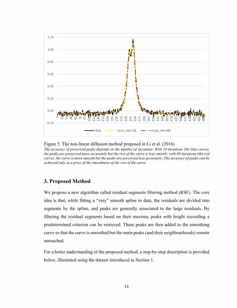
Figure 5. The non-linear diffusion method proposed in Li et al. (2016) ........................ 11 

Figure 6. Fitting a smoothing spline to the data .............................................................. 13 

Figure 7. Peaks and valleys to be preserved ................................................................... 14 

Figure 8. Components of the fitted curve........................................................................ 15 

Figure 9. Output of RSF algorithm. ................................................................................ 15 

Figure 10. Comparison between NDM and RSF method ............................................... 16 

Table 1. Comparison between NDM and RSF Methods by Mean Squared Error .......... 17 

Figure 11. Choice of λ ..................................................................................................... 18 

Figure 12. Effect of parameter h ..................................................................................... 19 

Figure 13. Identification of Kangaroo Tail pattern ......................................................... 20 

ix  

Foreword

Approval was received by the Master of Science in Management program to write this

thesis in English and under an article format. In addition, co-author’s approval was

obtained for using the article in this thesis. The article uses existing data collected for a

project approved by the Comité d'éthique de la recherche (CER).

A “peak” in this thesis refers to a peak or a valley, as the latter is considered a negative

peak and treated the same way as for a positive peak.

For the algorithms discussed in the thesis, the input data is an observational univariate

data set thus naturally discrete. Therefore, the resulting curve is referred as an empirical

curve which consists of interpolated observed data points, using a linear interpolation.

x  

Acknowledgements

I would firstly like to thank my thesis advisor, Professor Marc Fredette. He led me into

the world of data analysis and guided me through my studies and research. Without his

encouragement, direction and participation, this article would not exist.

I would also like to thank my colleague Amay Cheam, PhD. She proofread my article

several times and gave me detailed comments which rends the explanation in the article

more comprehensible and the text more readable.

1  

Introduction

My thesis proposes a method for peak-preserving curve smoothing called residual

segments filtering (RSF) method. This method allows to keep main peaks untouched

while greatly smoothing the rest of the data.

Why peak-preserving curve smoothing?

This topic is inspired by a problem that I encountered in my work as a data analyst. I work

in a user experience (UX) laboratory, where experiments are conducted to test participants

experience while doing diverse tasks using an interface. Data are collected using both

questionnaires and instruments which can detect and record various neurophysiological

signals of participants.

Let us consider a typical project under a within-subject design, where each participant is

asked to complete the same tasks under different conditions (versions A and B of a

company’s website, for example). While doing the tasks, participants’ electrodermal

activation (EDA, a measure of activation of an emotion), pupil dilation (a measure of

cognitive load) and facial emotional expressions (valence) are automatically recorded

with a fix frequency, 10 Hz for example (10 Hz = 10 measurements per second). Thus the

data is longitudinal and each participant’s EDA is a time series within a task. If aggregated

at participant and task level, the data is still longitudinal as each participant does multiple

tasks.

To compare these variables between conditions for a certain task, a regression with mixed

effect can be used. However, this approach exploits the central tendency and omits the

temporal information. For example, with website A, the difficulty level of a task increases

over time, while, with website B, it decreases. If their cognitive load is close to each other

on average over time, the regression will probably find no significant difference in the

cognitive load between the two websites even though users’ experience is very different.

To have a better understanding of the participants’ experience, temporal information is

instructive and needed. Such univariate longitudinal data can be represented by curves.

2  

One way to explore the curves is to regroup similar curves into the same groups, by a

family of techniques called curve clustering.

It may be worth noting that, when referring to observed data, a curve consists of observed

data points and linear interpolation between each two successive data points, as the

observation is at discrete times. This is applicable for observational data and unknown

distribution. Such curve is also called empirical curve throughout the thesis.

Curve clustering methods could be based on model or distance, with or without time

warping, all depends on the data and the purpose of the analysis. My study on curve

clustering starts with the simplest case where all the curves have x-axis (i.e. time)

synchronized - thus no time warping is needed - and similarity is defined by the shape of

curves without considering their amplitude. Thus, a distance-based correlation in

conjunction with the classical clustering algorithm is appropriate for such problem. The

distance is a transformation of Pearson correlation between each pair of curves.

This algorithm doesn’t require curve smoothing, however any irrelevant variations impact

the results as the noise does. This is especially true when the curves are expected to

contain some major peaks as consequence of some manipulated events, and we want to

focus on those peaks and take the rest as the context of the peaks. For example, in one of

the experiments, we are interested in participants’ reaction to violent movie scenes in

different cinema settings. We expect participants’ EDA goes up and down along the

movie. We expect especially a peak of EDA signal at the moment when a violent scene is

played. We are interested in the peak, but with a meaningful context. Participants’

activation level before the peak arrives, which we consider the context of the peak, can be

high or low, stable or turbulent. Thus we don’t want to ignore the context even though not

focus on it. That is, we want to study the peaks in great details and the context more

generally. This is when a peak preserving curve smoothing is needed: to preserve the

major peaks while greatly smooth the rest of the curves. In such scenario, classical curve

smoothing methods such as moving average or splines are not good candidates, as they

tend to smooth out everything including the peaks.

3  

In the literature, most of the existing peak preserved smoothing methods detect peaks by

analysing the variation of curvature: a peak is where the curvature varies abruptly(Irène

Gijbels, 2008; Hall & Titterington, 1992; McDonald & Owen, 1986; Hao et al., 2011; Li

et al., 2016). A threshold may be defined to filter out minor peaks. These algorithms then

change its behavior when it comes to the peaks and its near neighborhood so as to apply

less smoothing power in these areas. Although the aforementioned methods preserve the

peaks better than the classical smoothing methods, the peaks are more or less flattened.

As no existing method is found to be able to recognize the major peaks and keep them

untouched without reducing its smoothing capacity for the rest of the curve, I focused my

research on dealing with this problem.

Why residual segments filtering?

The initial purpose of developing this method was for curve clustering, therefore it is

natural that we wanted to preserve peaks with their neighborhood, as the shape was our

main interest.

By fitting a smoothing spline to an empirical curve, a peak with its neighborhood becomes

a segment of residuals. Adding all the residuals to the spline, we return back to the

empirical curve; but instead if we only added the major peaks to the spline, we obtain a

smoothed curve with untouched peaks. This is the core of the RSF method.

Parameters of the method

The performance of this method depends on two parameters controlling the smoothness

of the curve and peaks to be preserved respectively. In fact, the first one is , the tuning

parameter for the smoothing spline (Ryan Tibshirani, 2014), controlling the degree of

penalization of the variation of curvature as discussed in Section 3. The second is the

minimum peak height - peaks higher than which will be preserved. To make second

parameter a bit more adaptive to data, it is modified to a multiple of the standard deviation

of the residuals.

Applicability of the method

4  

The proposed method is applicable to any univariate longitudinal data. It can be used for

peak-preserving curve smoothing as its name suggests and as described in great details in

the first sections of the article. It can also be used as a peak finder to filter and retrieve

peaks with neighborhood. Unlike the conventional way, peaks are not defined by its

distance to a static base, e.g. 0, but instead by its height relative to the spline which

represents the empirical curve’s general shape. The philosophy is that, we let the spline

to capture the general pattern, and the peaks to capture short-term irregular fluctuation

that is out of the reach of the spline.

In cases where peaks are likely to be caused by noise, this method is not suitable. At times

when peaks are likely to be real signal but may contain noise, users must keep in mind

that this method doesn’t reduce noise in the near neighbourhood of preserved peaks. The

use of this method is best justified when there is relatively irrelevant information but no

concerns of noise, as in the case of finding Kangaroo-tails in a candlestick chart of stock

price illustrated in Section 6.

5  

The article: A Peak-Preserving Curve Smoothing method

Shang Lin Chen, Marc Fredette

HEC Montréal, Tech3Lab, 3000 Chemin de la Côte-Sainte-Catherine, Montréal, Québec, Canada, H3T 2A7

Abstract

In time series analysis, when we are particularly interested in peaks and consider the rest less relevant, techniques to smooth the empirical curve (consisting of observations and linear interpolation between two successive observations) while preserving significant peaks with high accuracy may be needed. This paper proposes a method to solve this type of problems. The general pattern is obtained by fitting a smoothing spline to the data where highest peaks (and deepest valleys) are retrieved with their neighborhood by filtering the residuals. Peak features such as location, summit and shape can thus be preserved, allowing further analysis based on the shape of peaks. This method can also be used as a detection procedure in order to retrieve significant peaks in a time series dataset.

Keywords: smoothing spline, peak preserving, peak detector, short-term fluctuation 1. Motivating Application

Vibro-kinetic movie experience refers to dynamic chairs that move in synchronization

with the movie scenes. For instance, the seat remains still during a peaceful scene but

suddenly generate a trembling motion when an earthquake scene appears to provide users

with a more immersive experience than traditional ones.

In an experiment for evaluating the effect of vibro-kinetic movie seats on the user’s

experience, participants were randomly assigned to different groups to watch the same

movies but using different seats (vibro-kinetic or traditional seats). As an indicator of the

intensity of emotion (Lang et al., 1993), the electrodermal activity (EDA, in microsiemens

μS) of the participants is measured. With time represented on the x-axis and EDA on the

y-axis, we get a “curve” for each participant during each movie. Note that such an

empirical curve consists of a sequence of observed data points and linear interpolation

between two successive data points. As these curves represent the evolution of

participants’ emotion intensity which is an important aspect of participants’ experience,

we want to cluster the participants based on these EDA curves.

6  

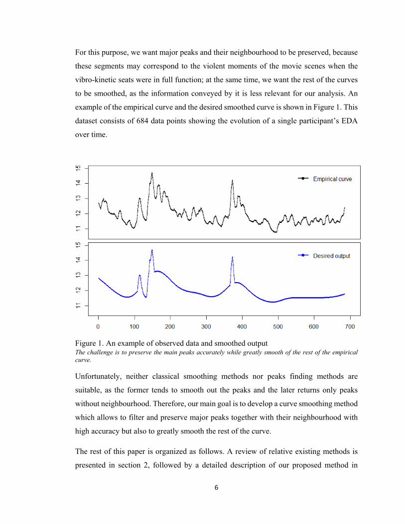
For this purpose, we want major peaks and their neighbourhood to be preserved, because

these segments may correspond to the violent moments of the movie scenes when the

vibro-kinetic seats were in full function; at the same time, we want the rest of the curves

to be smoothed, as the information conveyed by it is less relevant for our analysis. An

example of the empirical curve and the desired smoothed curve is shown in Figure 1. This

dataset consists of 684 data points showing the evolution of a single participant’s EDA

over time.

Figure 1. An example of observed data and smoothed output The challenge is to preserve the main peaks accurately while greatly smooth of the rest of the empirical curve.

Unfortunately, neither classical smoothing methods nor peaks finding methods are

suitable, as the former tends to smooth out the peaks and the later returns only peaks

without neighbourhood. Therefore, our main goal is to develop a curve smoothing method

which allows to filter and preserve major peaks together with their neighbourhood with

high accuracy but also to greatly smooth the rest of the curve.

The rest of this paper is organized as follows. A review of relative existing methods is

presented in section 2, followed by a detailed description of our proposed method in

7  

section 3. In section 4, we compare our method with the non-linear diffusion method

introduced in Li et al. (2016), which is recent and produces results close to ours. The

choice of parameter of our method is then discussed in section 5. In section 6, we discuss

the possibility of using this method as peak finder. Then we conclude and suggest further

studies in section 7.

2. Existing Methods

To the best of our knowledge, there is no existing algorithm available in the literature is

suitable for our purpose explained in Section 1. In fact, most of the existing peak-

preserving methods either more or less smooth out the peaks, or keep only the peaks

without neighbourhood.

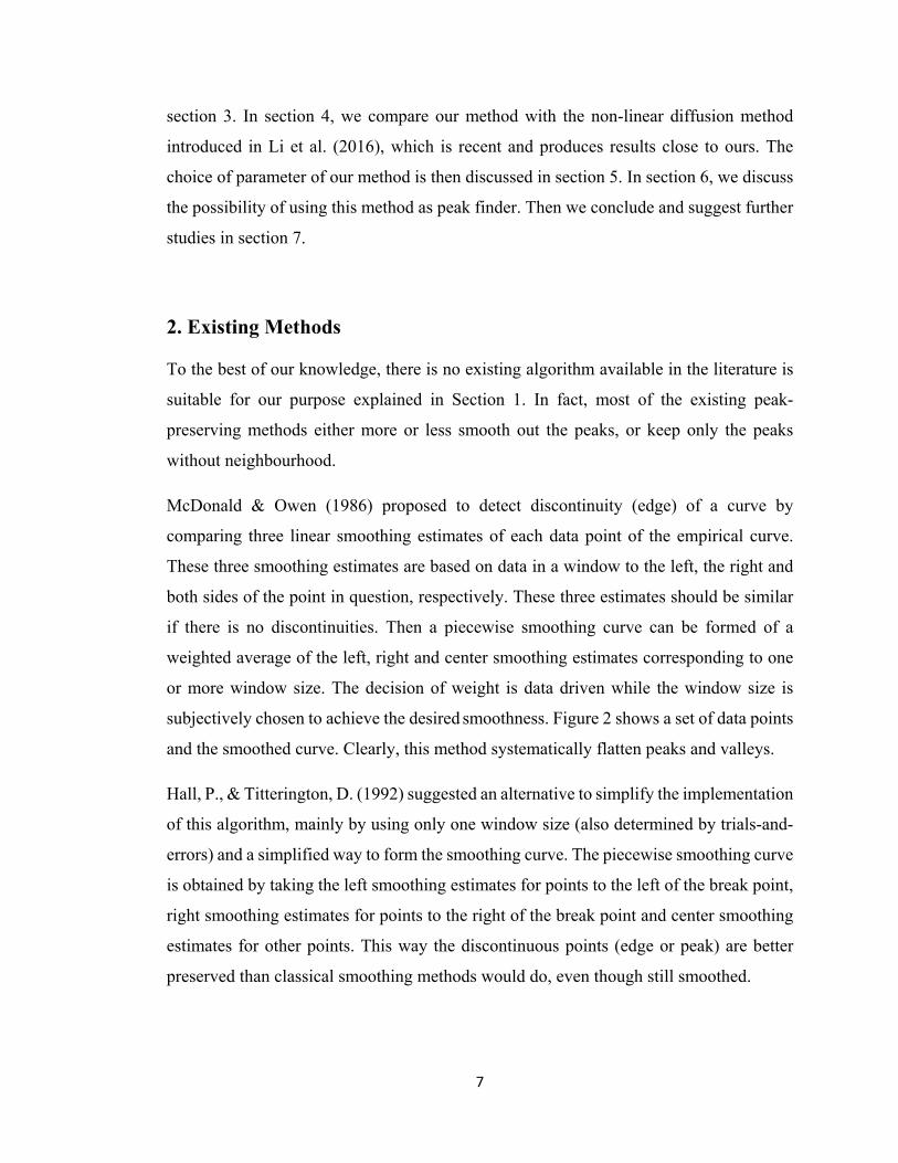
McDonald & Owen (1986) proposed to detect discontinuity (edge) of a curve by

comparing three linear smoothing estimates of each data point of the empirical curve.

These three smoothing estimates are based on data in a window to the left, the right and

both sides of the point in question, respectively. These three estimates should be similar

if there is no discontinuities. Then a piecewise smoothing curve can be formed of a

weighted average of the left, right and center smoothing estimates corresponding to one

or more window size. The decision of weight is data driven while the window size is

subjectively chosen to achieve the desired smoothness. Figure 2 shows a set of data points

and the smoothed curve. Clearly, this method systematically flatten peaks and valleys.

Hall, P., & Titterington, D. (1992) suggested an alternative to simplify the implementation

of this algorithm, mainly by using only one window size (also determined by trials-and-

errors) and a simplified way to form the smoothing curve. The piecewise smoothing curve

is obtained by taking the left smoothing estimates for points to the left of the break point,

right smoothing estimates for points to the right of the break point and center smoothing

estimates for other points. This way the discontinuous points (edge or peak) are better

preserved than classical smoothing methods would do, even though still smoothed.

8  

Figure 2. Method proposed by McDonald & Owen (1986) This is Figure 16 in McDonald & Owen (1986). This algorithm preserves peaks better than classical smoothing methods would do, but peaks are still blurred. Clearly, this method is not suitable for our case as our goal is to achieve both smoothness of the curve and accuracy of the peak.

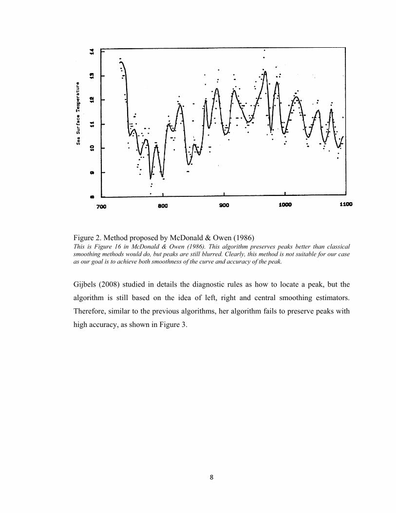
Gijbels (2008) studied in details the diagnostic rules as how to locate a peak, but the

algorithm is still based on the idea of left, right and central smoothing estimators.

Therefore, similar to the previous algorithms, her algorithm fails to preserve peaks with

high accuracy, as shown in Figure 3.

9  

Figure 3. Method proposed by Gijbels (2008) This is Figure 4.1 in Gijbels (2008). The thin solid curve is the true curve, the dotted and dashed curves are two fitted curves with different window sizes. With smaller window size, the peak is better preserved (though still smoothed) but the curve is less smooth elsewhere. Clearly, this method is not a good candidate as our goal is to achieve both smoothness of the curve and accuracy of the peak.

Hao et al. (2011) used a variant of the Ramer–Douglas–Peucker algorithm (Ramer, 1972;

Douglas & Peucker, 1973) which reduces a curve to its most significant data points

connected by lines. The particularity of this method is that peaks are not detected by

analysing the variation of curvature, but instead by filtering the residuals of a fitted model,

where the model is simply a line connecting the first and the last points of the curve at

each iteration. Figure 4 shows that this algorithm succeeds at preserving the peaks but

fails to keep its neighbourhood and any information between peaks.

10  

Figure 4. A variant of the Ramer–Douglas–Peucker algorithm This figure is reproduced for a better resolution based on Figure 3 of Hao et al. (2011). The curve is reduced to its most significant data points (start point, end point and peaks exceeding a certain height) connected by lines.

Li et al. (2016) proposed an image processing method for peak-preserving curve

smoothing called non-linear diffusion (NDM). Peaks are defined as locations with large

curvature variation rate. The algorithm is forced to smooth with less strength at these

locations. As shown in Figure 5, this method achieves a good smoothness of the curve

with good accuracy of the peak. However, the preserved peaks are more or less flattened.

One can vary the number of iterations to find a balance between the smoothness of curve

and the accuracy of peaks. To the best of our knowledge, this method is the latest and the

closest to solve the mentioned problem. Thus it will be compared with our method in

Section 4.

0 1 2 3 4 5 6 7 8 9 10 11 12 13 14

Input Output

11  

  

Figure 5. The non-linear diffusion method proposed in Li et al. (2016) The accuracy of preserved peaks depends on the number of iterations. With 10 iterations (the blue curve), the peaks are preserved more accurately but the rest of the curve is less smooth; with 80 iterations (the red curve), the curve is more smooth but the peaks are preserved less accurately. The accuracy of peaks can be achieved only at a price of the smoothness of the rest of the curve.

3. Proposed Method

We propose a new algorithm called residual segments filtering method (RSF). The core

idea is that, while fitting a “very” smooth spline to data, the residuals are divided into

segments by the spline, and peaks are generally associated to the large residuals. By

filtering the residual segments based on their maxima, peaks with height exceeding a

predetermined criterion can be retrieved. These peaks are then added to the smoothing

curve so that the curve is smoothed but the main peaks (and their neighbourhoods) remain

untouched.

For a better understanding of the proposed method, a step-by-step description is provided

below, illustrated using the dataset introduced in Section 1.

‐0.15

0.05

0.25

0.45

0.65

0.85

1.05

1.25

1

16

31

46

61

76

91

106

121

136

151

166

181

196

211

226

241

256

271

286

301

316

331

346

361

376

391

406

421

436

451

466

481

Raw num_iter=10 num_iter=80

12  

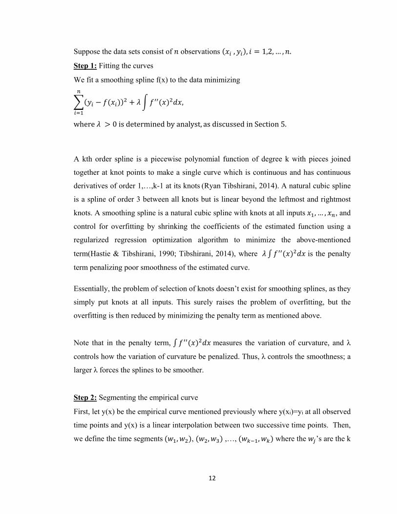
Suppose the data sets consist of observations , , 1,2, … , .

Step 1: Fitting the curves

We fit a smoothing spline f(x) to the data minimizing

,

where 0isdeterminedbyanalyst, asdiscussedinSection5.

A kth order spline is a piecewise polynomial function of degree k with pieces joined

together at knot points to make a single curve which is continuous and has continuous

derivatives of order 1,…,k-1 at its knots (Ryan Tibshirani, 2014). A natural cubic spline

is a spline of order 3 between all knots but is linear beyond the leftmost and rightmost

knots. A smoothing spline is a natural cubic spline with knots at all inputs , … , , and

control for overfitting by shrinking the coefficients of the estimated function using a

regularized regression optimization algorithm to minimize the above-mentioned

term(Hastie & Tibshirani, 1990; Tibshirani, 2014), where is the penalty

term penalizing poor smoothness of the estimated curve.

Essentially, the problem of selection of knots doesn’t exist for smoothing splines, as they

simply put knots at all inputs. This surely raises the problem of overfitting, but the

overfitting is then reduced by minimizing the penalty term as mentioned above.

Note that in the penalty term, measures the variation of curvature, and λ

controls how the variation of curvature be penalized. Thus, λ controls the smoothness; a

larger λ forces the splines to be smoother.

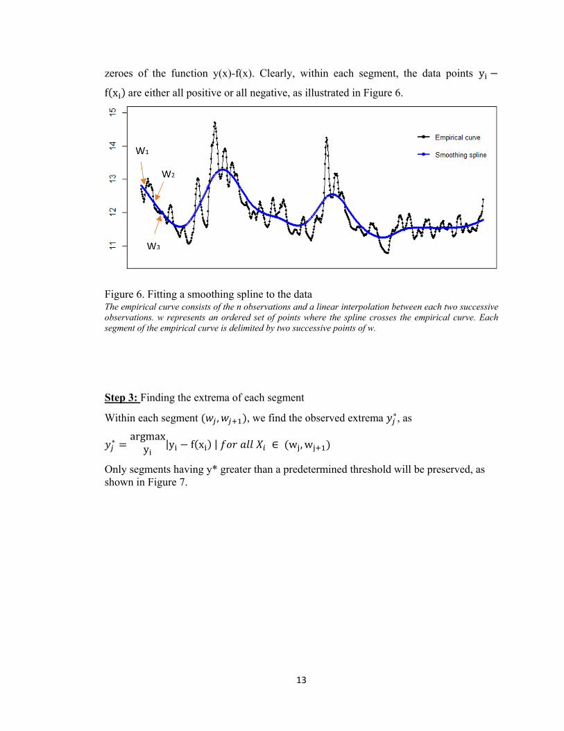
Step 2: Segmenting the empirical curve

First, let y(x) be the empirical curve mentioned previously where y(xi)=yi at all observed

time points and y(x) is a linear interpolation between two successive time points. Then,

we define the time segments , , , ,…, , where the ’s are the k

13  

zeroes of the function y(x)-f(x). Clearly, within each segment, the data points y

f x are either all positive or all negative, as illustrated in Figure 6.

Figure 6. Fitting a smoothing spline to the data The empirical curve consists of the n observations and a linear interpolation between each two successive observations. w represents an ordered set of points where the spline crosses the empirical curve. Each segment of the empirical curve is delimited by two successive points of w.

 

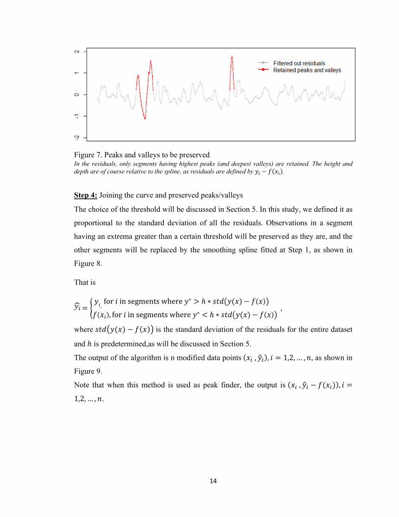
Step 3: Finding the extrema of each segment

Within each segment , , we find the observed extrema ∗, as

∗ argmaxy |y f x | ∈ w ,w

Only segments having y* greater than a predetermined threshold will be preserved, as shown in Figure 7.

14  

Figure 7. Peaks and valleys to be preserved In the residuals, only segments having highest peaks (and deepest valleys) are retained. The height and depth are of course relative to the spline, as residuals are defined by .

Step 4: Joining the curve and preserved peaks/valleys

The choice of the threshold will be discussed in Section 5. In this study, we defined it as

proportional to the standard deviation of all the residuals. Observations in a segment

having an extrema greater than a certain threshold will be preserved as they are, and the

other segments will be replaced by the smoothing spline fitted at Step 1, as shown in

Figure 8.

That is

,for insegmentswhere ∗ ∗

, for insegmentswhere ∗ ∗,

where is the standard deviation of the residuals for the entire dataset

and is predetermined,as will be discussed in Section 5.

The output of the algorithm is n modified data points , , 1,2, … , , as shown in

Figure 9.

Note that when this method is used as peak finder, the output is , ,

1,2, … , .

15  

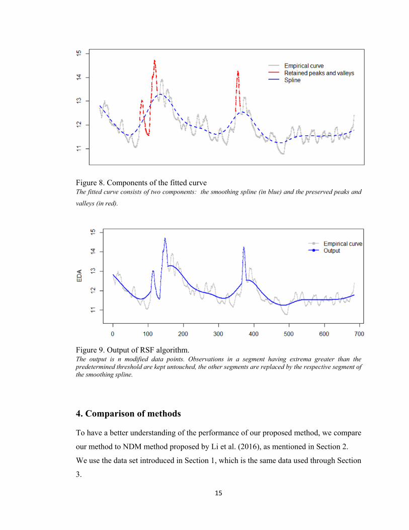
Figure 8. Components of the fitted curve The fitted curve consists of two components: the smoothing spline (in blue) and the preserved peaks and

valleys (in red).

Figure 9. Output of RSF algorithm. The output is n modified data points. Observations in a segment having extrema greater than the predetermined threshold are kept untouched, the other segments are replaced by the respective segment of the smoothing spline.

4. Comparison of methods

To have a better understanding of the performance of our proposed method, we compare

our method to NDM method proposed by Li et al. (2016), as mentioned in Section 2.

We use the data set introduced in Section 1, which is the same data used through Section

3.

16  

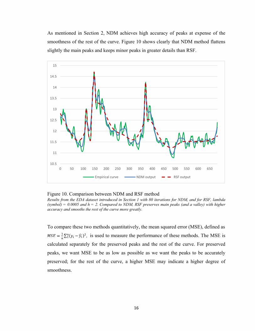
As mentioned in Section 2, NDM achieves high accuracy of peaks at expense of the

smoothness of the rest of the curve. Figure 10 shows clearly that NDM method flattens

slightly the main peaks and keeps minor peaks in greater details than RSF.

Figure 10. Comparison between NDM and RSF method Results from the EDA dataset introduced in Section 1 with 80 iterations for NDM, and for RSF, lambda (symbol) = 0.0005 and h = 2. Compared to NDM, RSF preserves main peaks (and a valley) with higher accuracy and smooths the rest of the curve more greatly.

To compare these two methods quantitatively, the mean squared error (MSE), defined as

is used to measure the performance of these methods. The MSE is

calculated separately for the preserved peaks and the rest of the curve. For preserved

peaks, we want MSE to be as low as possible as we want the peaks to be accurately

preserved; for the rest of the curve, a higher MSE may indicate a higher degree of

smoothness.

10.5

11

11.5

12

12.5

13

13.5

14

14.5

15

0 50 100 150 200 250 300 350 400 450 500 550 600 650

Empirical curve NDM output RSF output

17  

Table 1. Comparison between NDM and RSF Methods by Mean Squared Error Peaks & valleys preserved

by RSF The rest of the curve

Nonlinear Diffusion Method (NDM) 0.110

0.027

Residual segment filtering method (RSF)

0 0.077

For peaks preserved by RSF, the MSE is 0 for RSF and 0.110 for NDM, which confirms

that RSF preserved peaks untouched while NDM modified the peaks. For the rest of the

curves, RSF has higher MSE than NDM, which indicates that RSF is smoother than NDM

in sections where no peaks are to be preserved.

In sum, compared to NDM, we feel that our method performs significantly better because

1) It allows to filter peaks, only the highest peaks and deepest valleys are preserved.

2) It allows to keep selected peaks untouched.

3) The rest of the curve can be greatly smoothed.

Note that the premise of the comparison is that RSF preserves the “right” peaks. In fact,

RSF preserves the peaks which are among the highest, relative to their neighbourhood. In

other words, it’s not the global maxima but the local maxima that RSF preserves. In

practice, this can be short term fluctuations of stock price, temperature, etc. If such peaks

are the peaks of interest, then RSF can preserve the right peaks – and this is the case where

RSF becomes useful. If such peaks are likely to be caused by undesired outliers or noise,

then RSF is not the good method to use, as it will preserve these outliers and it does not

reduce noise in the near neighbourhood of preserved peaks.

5. Choice of parameters

To produce a better result, both the smoothness of the spline and the threshold for filtering

the peaks are important.

The smoothness of the spline is controlled by the parameter . A larger penalize more

the variation of curvature thus force the spline to be smoother. Figure 11 shows three

splines with different fitted to the same data using the smooth.spline() function in R

version 3.4.3(R Core Team, 2017). It shows clearly that splines generated with larger are

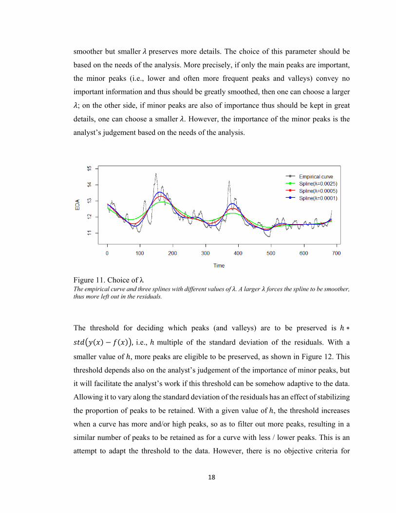
18  

smoother but smaller preserves more details. The choice of this parameter should be

based on the needs of the analysis. More precisely, if only the main peaks are important,

the minor peaks (i.e., lower and often more frequent peaks and valleys) convey no

important information and thus should be greatly smoothed, then one can choose a larger

; on the other side, if minor peaks are also of importance thus should be kept in great

details, one can choose a smaller . However, the importance of the minor peaks is the

analyst’s judgement based on the needs of the analysis.

Figure 11. Choice of λ The empirical curve and three splines with different values of . A larger forces the spline to be smoother, thus more left out in the residuals.

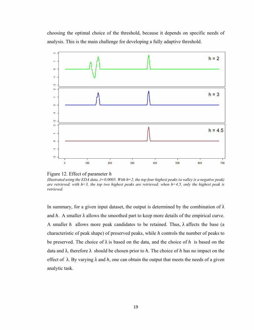
The threshold for deciding which peaks (and valleys) are to be preserved is ∗

, i.e., multiple of the standard deviation of the residuals. With a

smaller value of , more peaks are eligible to be preserved, as shown in Figure 12. This

threshold depends also on the analyst’s judgement of the importance of minor peaks, but

it will facilitate the analyst’s work if this threshold can be somehow adaptive to the data.

Allowing it to vary along the standard deviation of the residuals has an effect of stabilizing

the proportion of peaks to be retained. With a given value of , the threshold increases

when a curve has more and/or high peaks, so as to filter out more peaks, resulting in a

similar number of peaks to be retained as for a curve with less / lower peaks. This is an

attempt to adapt the threshold to the data. However, there is no objective criteria for

19  

choosing the optimal choice of the threshold, because it depends on specific needs of

analysis. This is the main challenge for developing a fully adaptive threshold.

Figure 12. Effect of parameter Illustrated using the EDA data, λ=0.0005. With h=2, the top four highest peaks (a valley is a negative peak) are retrieved; with h=3, the top two highest peaks are retrieved; when h=4.5, only the highest peak is retrieved.

In summary, for a given input dataset, the output is determined by the combination of λ

and . A smaller λ allows the smoothed part to keep more details of the empirical curve.

A smaller allows more peak candidates to be retained. Thus, λ affects the base (a

characteristic of peak shape) of preserved peaks, while controls the number of peaks to

be preserved. The choice of λ is based on the data, and the choice of is based on the

data and λ, therefore λ should be chosen prior to . The choice of has no impact on the

effect of λ. By varying λ and , one can obtain the output that meets the needs of a given

analytic task.

 

20  

6. Other Applications

RSF is a general method applicable to univariate data when a curve needs to be smoothed

and the highest peaks and their neighbourhood need to be preserved. This has been

illustrated in great details in the previous sections. Figure 12 suggests that this method

also has the potential to identify and filter peaks. In this section we discuss its use as a

peak finder.

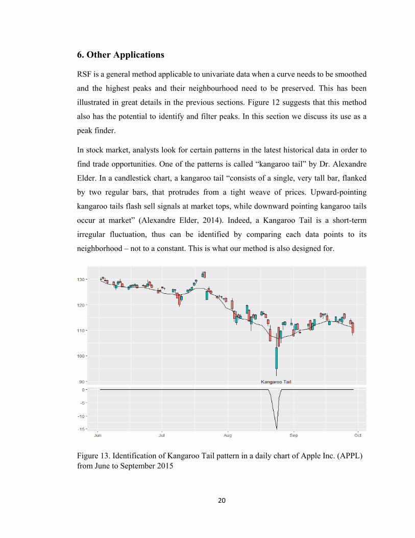
In stock market, analysts look for certain patterns in the latest historical data in order to

find trade opportunities. One of the patterns is called “kangaroo tail” by Dr. Alexandre

Elder. In a candlestick chart, a kangaroo tail “consists of a single, very tall bar, flanked

by two regular bars, that protrudes from a tight weave of prices. Upward-pointing

kangaroo tails flash sell signals at market tops, while downward pointing kangaroo tails

occur at market” (Alexandre Elder, 2014). Indeed, a Kangaroo Tail is a short-term

irregular fluctuation, thus can be identified by comparing each data points to its

neighborhood – not to a constant. This is what our method is also designed for.

Figure 13. Identification of Kangaroo Tail pattern in a daily chart of Apple Inc. (APPL) from June to September 2015

21  

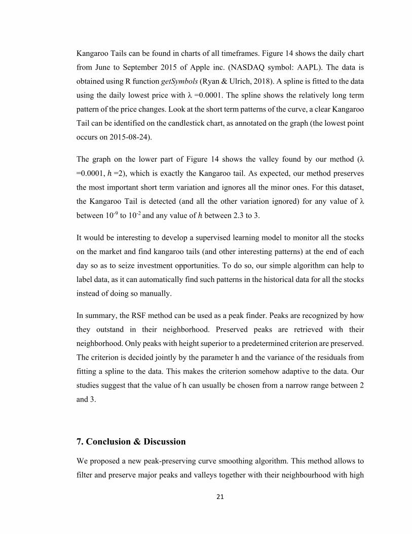
Kangaroo Tails can be found in charts of all timeframes. Figure 14 shows the daily chart

from June to September 2015 of Apple inc. (NASDAQ symbol: AAPL). The data is

obtained using R function getSymbols (Ryan & Ulrich, 2018). A spline is fitted to the data

using the daily lowest price with λ =0.0001. The spline shows the relatively long term

pattern of the price changes. Look at the short term patterns of the curve, a clear Kangaroo

Tail can be identified on the candlestick chart, as annotated on the graph (the lowest point

occurs on 2015-08-24).

The graph on the lower part of Figure 14 shows the valley found by our method (λ

=0.0001, =2), which is exactly the Kangaroo tail. As expected, our method preserves

the most important short term variation and ignores all the minor ones. For this dataset,

the Kangaroo Tail is detected (and all the other variation ignored) for any value of λ

between 10-9 to 10-2 and any value of between 2.3 to 3.

It would be interesting to develop a supervised learning model to monitor all the stocks

on the market and find kangaroo tails (and other interesting patterns) at the end of each

day so as to seize investment opportunities. To do so, our simple algorithm can help to

label data, as it can automatically find such patterns in the historical data for all the stocks

instead of doing so manually.

In summary, the RSF method can be used as a peak finder. Peaks are recognized by how

they outstand in their neighborhood. Preserved peaks are retrieved with their

neighborhood. Only peaks with height superior to a predetermined criterion are preserved.

The criterion is decided jointly by the parameter h and the variance of the residuals from

fitting a spline to the data. This makes the criterion somehow adaptive to the data. Our

studies suggest that the value of h can usually be chosen from a narrow range between 2

and 3.

7. Conclusion & Discussion

We proposed a new peak-preserving curve smoothing algorithm. This method allows to

filter and preserve major peaks and valleys together with their neighbourhood with high

22  

accuracy, while greatly smooth the rest of the curve. For this purpose, our method

performs better than existing methods. Furthermore, our approach, which is totally

different from any of the existing methods, could be an inspiration for future studies.

This method is rather flexible as the smoothness of fitted curve and the threshold of peaks

to be preserved can be decided by analysts. The fact that the neighbourhood of peaks are

preserved is important especially if further peak analysis based on the shape of peaks need

to be performed.

Contrast to most of the existing methods which detect peaks by analyzing the variation of

curvature, our method is based on analysis of residuals. In this sense it can be considered

as a variant of the method proposed by Hao et al, as reviewed in Section 2. The key

difference is that, in Hao’s method, the fitted curve is a straight line connecting the start

point to the end point, while in our algorithm it is a smoothing spline. Thus, our algorithm

captures more information about the neighborhood of peaks as well as the general pattern

of the curve. From implementation point of view, Hao’s algorithm is iterative while ours

is not.

The non-linear diffusion algorithm proposed by Li et al. (2016) seems to produce similar

results to ours, but it achieves high accuracy of peaks at the expense of poor smoothness

of the rest of the curve, unlike our method which allows to keep peaks untouched while

greatly smooth the rest of the curve, as discussed in Section 4.

Further studies

The determination of and is critical for satisfactory results. Obviously, the optimal

value of and for a given curve depends on two factors: the objective of the analysis

and the characteristics of the empirical curve. Currently it is supposed to be determined

by a trial-and-error method to obtain a curve satisfying the specific purpose of analysis.

Making these parameters more adaptive to the data is an asset to the method. A plausible

idea is to allow to vary proportionally to the variance of the residuals. A good starting

point is to set =2, but further studies are needed to make these parameters more adaptive

to data.

23  

References

[1] Alexandre Elder (2014), “The New Trading For Living”. John Wiley & Sons, Inc., Hoboken, New Jersey. ISBN: 9781118963678. P.67.

[2] David Douglas & Thomas Peucker, “Algorithms for the reduction of the number of points required to represent a digitized line or its caricature”. The Canadian Cartographer 10(2), 112–122 (1973) doi:10.3138/FM57-6770-U75U-7727

[3] Irène Gijbels (2008). “Smoothing and preservation of irregularities using local linear fitting”. Applications of Mathematics. 53. 177-194. 10.1007/s10492-008-0003-3.

[4] Peter Hall & Michael Titterington (1992). “Edge-Preserving and Peak-Preserving Smoothing”. Technometrics, 34(4), 429-440. doi:10.2307/1268942

[5] Trevor Hastie & Robert Tibshirani (1990). “Generalized Additive Models”. Chapman and Hall.

[6] Horea Pauna, Pierre-Majorique Léger, Sylvain Sénécal, Marc Fredette, François Courtemanche, Shang-Lin Chen, Élise Labonté-Lemoyne1 and Jean-François Ménard. (2018). “The Psychophysiological Effect of a Vibro-Kinetic Movie Experience: The Case of the D-BOX Movie Seat”. In Information Systems and Neuroscience. Springer, Berlin, 1-7.

[7] Lang, Peter J., Mark K. Greenwald, Margaret M. Bradley and Alfons O. Hamm (1993). “Looking at pictures: Affective, facial, visceral, and behavioral reactions”. Psychophysiology 30, no. 3, p. 261-273.

[8] Jeffrey A. Ryan and Joshua M. Ulrich (2018). quantmod: Quantitative Financial Modelling Framework. R package version 0.4-13. https://CRAN.R-project.org/package=quantmod

[9] John Alan McDonald & Art B. Owen (1986). “Smoothing with Split Linear Fits”. Technometrics, 28(3), 195-208. doi:10.2307/1269075

[10] M. C. Hao, H. Janetzko, S. Mittelstädt, W. Hill, U. Dayal, D. A. Keim, M. Marwah, R. K. Sharma(2011) “A Visual Analytics Approach for Peak-Preserving Prediction of Large Seasonal Time Series”, Computer Graphics Forum, June 2011, DOI: 10.1111/j.1467-8659.2011.01918.x

[11] R Core Team (2017). “R: A language and environment for statistical computing”. R Foundation for Statistical Computing, Vienna, Austria. URL https://www.R-project.org/.

[12] Ryan Tibshirani (2014). “Nonparametric regression”. Statistical Machine Learning, Spring 2015

[13] Urs Ramer, "An iterative procedure for the polygonal approximation of plane curves", Computer Graphics and Image Processing, 1(3), 244–256 (1972) doi:10.1016/S0146-664X(72)80017-0

24  

[14] Yuanlu Li, Yaqing Ding and Tiao Li (2016). “Nonlinear diffusion filtering for peak-preserving smoothing of a spectrum signal”. Chemometrics and Intelligent Laboratory Systems, v.156, 2016 August 15, p.157(9) (ISSN: 0169-7439)

 

25  

Conclusion

Review of the method

This paper proposed the RSF method, a peak preserving curve smoothing method for time

series. This method is based on smoothing spline and residual segments filtering. By

filtering the residual segments, the major peaks and valleys, as well as their

neighbourhood are recognized and kept untouched, while the rest of the curve is smoothed

by a spline. The smoothness of the curve is controlled by the parameter , and the

eligibility criterion for a peak to be preserved is controlled by the parameter . and

are determined by the analyst according to the needs for peaks to be preserved and the

smoothness of the fitted curve.

While existing peak preserving curve smoothing methods find peaks by analyzing the

variation of the curvature, the RSF takes a fundamentally different approach to detect

major peaks: it considers residuals as segments, and filter the segments by their extrema;

if an extrema exceeds the criterion, then the entire segment is preserved. This approach

brings some advantages and limitations to the proposed method.

Advantages

Firstly, the preserved peak remains untouched. In other words, peaks are preserved with

100% accuracy.

Secondly, if a peak is preserved, it is preserved with its neighborhood. Therefore not only

the location and value of the peak (the extrema), but also the shape of the peak (i.e., its

neighborhood) is preserved, which open the door to further analysis based on the shape

of peak.

Also, the capacity to preserve peaks does not affect the capacity to smooth the rest of the

curve. One does not need to compromise between the accuracy of peaks and smoothness

of the curve.

26  

Limitations

A peak is preserved with its neighborhood, where the extent of neighbourhood is

determined by the smoothing spline. For peaks having clear starting points (where the

curvature increases abruptly), the preserved neighborhood starts generally at a point

higher than that starting point. This is not necessarily bad for curve clustering tasks, as

the upper part of the peak conveys most important information, and the lower part is

somehow captured by the spline. However, this is not optimal for analysis based on the

shape of peak.

Another limitation is the assumption that: 1) the spline captures the general pattern, and

2) the preserved peaks add specific information to the spline; while at the beginning the

spline has already been affected by the peaks itself that are later preserved and added.

Thus the preserved peaks are over emphasized in the fitted curve. However, the most

serious impact of a preserved peak to the spline happens to the segment where the peak

exists, but this segment of spline is later replaced by the peak and its neighborhood thus

not part of the fitted curve. Therefore the effect of this limitation might be negligible.

Future study

The choice of parameters and h is important for satisfactory results. The optimal values

of the parameters depend on both the objective of the analysis and the characteristics of

the empirical curve. Currently it is supposed to be determined by a trial-and-error method

to obtain a curve satisfying the specific purpose of analysis. It will be useful if these

parameters are adaptive to data. Allowing to vary proportionally to the variance of the

empirical data seems to be a good starting point, further studies are needed to make these

parameters better adaptable to data.

27  

Bibliography

[1] Alexandre Elder (2014), “The New Trading For Living”. John Wiley & Sons, Inc., Hoboken, New Jersey. ISBN: 9781118963678. P.67.

[2] David Douglas & Thomas Peucker, “Algorithms for the reduction of the number of points required to represent a digitized line or its caricature”. The Canadian Cartographer 10(2), 112–122 (1973) doi:10.3138/FM57-6770-U75U-7727

[3] Irène Gijbels (2008). “Smoothing and preservation of irregularities using local linear fitting”. Applications of Mathematics. 53. 177-194. 10.1007/s10492-008-0003-3.

[4] Peter Hall & Michael Titterington (1992). “Edge-Preserving and Peak-Preserving Smoothing”. Technometrics, 34(4), 429-440. doi:10.2307/1268942

[5] Trevor Hastie & Robert Tibshirani (1990). “Generalized Additive Models”. Chapman and Hall.

[6] Horea Pauna, Pierre-Majorique Léger, Sylvain Sénécal, Marc Fredette, François Courtemanche, Shang-Lin Chen, Élise Labonté-Lemoyne1 and Jean-François Ménard. (2018). “The Psychophysiological Effect of a Vibro-Kinetic Movie Experience: The Case of the D-BOX Movie Seat”. In Information Systems and Neuroscience. Springer, Berlin, 1-7.

[7] Lang, Peter J., Mark K. Greenwald, Margaret M. Bradley and Alfons O. Hamm (1993). “Looking at pictures: Affective, facial, visceral, and behavioral reactions”. Psychophysiology 30, no. 3, p. 261-273.

[8] Jeffrey A. Ryan and Joshua M. Ulrich (2018). quantmod: Quantitative Financial Modelling Framework. R package version 0.4-13. https://CRAN.R-project.org/package=quantmod

[9] John Alan McDonald & Art B. Owen (1986). “Smoothing with Split Linear Fits”. Technometrics, 28(3), 195-208. doi:10.2307/1269075

[10] M. C. Hao, H. Janetzko, S. Mittelstädt, W. Hill, U. Dayal, D. A. Keim, M. Marwah, R. K. Sharma(2011) “A Visual Analytics Approach for Peak-Preserving Prediction of Large Seasonal Time Series”, Computer Graphics Forum, June 2011, DOI: 10.1111/j.1467-8659.2011.01918.x

[11] R Core Team (2017). “R: A language and environment for statistical computing”. R Foundation for Statistical Computing, Vienna, Austria. URL https://www.R-project.org/.

[12] Ryan Tibshirani (2014). “Nonparametric regression”. Statistical Machine Learning, Spring 2015

[13] Urs Ramer, "An iterative procedure for the polygonal approximation of plane curves", Computer Graphics and Image Processing, 1(3), 244–256 (1972) doi:10.1016/S0146-664X(72)80017-0

28  

[14] Yuanlu Li, Yaqing Ding and Tiao Li (2016). “Nonlinear diffusion filtering for peak-preserving smoothing of a spectrum signal”. Chemometrics and Intelligent Laboratory Systems, v.156, 2016 August 15, p.157(9) (ISSN: 0169-7439)

 

i  

Annex : R Code implementing the algorithm

# df: the input univariate data, also called empirical data in the text;

# lambda: controlling the smoothness of the spline. It is the same lambda

# as used in the R function smooth.spline();

# h: deciding the minimal peak height (valley depth) for a peak (valley)

# to be preserved.

smooth.peak = function(df, lambda, h) { # fit a smoothing spline to the data

base = smooth.spline(df, lambda=lambda)$y # find starting and end points of each segment, that is where the sign of residual changes

x = which ( diff (sign (df-base))!=0)

df2=df

for( i in 1: (length(x)-1)){ # find the extrema of each segment

max = ifelse (max ( df [x[i]:x[i+1] ] ) > max ( df [x[i]],

df[x[i+1]]), max ((df-base) [x[i]:x[i+1]]),

min((df-base)[x[i]:x[i+1]])) # filtering segments by their extrema

if(abs(max)< h*sd(df-base)){

df2[x[i]:x[i+1]]=base[x[i]:x[i+1]]

}

} # Use the spine at the starting and the ending point of the empirical data

df2[1:x[1]]=base[1:x[1]]

df2[x[length(x)]:length(df2)]=base[x[length(x)]:length(base)]

peaks=df2-base # preserved peaks

# return the peak-preserved smoothed curve(df2), the preserved peaks and the spline

return( list( df2, peaks, base)) }