thesis12122008 bound a4 - university of leicester · chapter 5 5
TRANSCRIPT
Chapter 5
Precursors and long quiescent times in
Swift GRBs
The current observational status of GRBs appears to show that their emission follows a canonical
behaviour, as seen in previous chapters of this work. However, one debated feature briefly mentioned
in §1.2.1 but not described in §1.3.3 is ‘precursor’ emission. The earliest theoretical models (Colgate,
1973, 1974) predicted that there may be some signature emission that occurs before the main phase
0 emission, which may have a separate physical origin and therefore spectral signature. This chapter
explores the definition of a ‘precursor’, describes the historical, theoretical and observational status of
such events and characterises quiescent periods within phase 0 emission. I then proceed to define my
own selection criteria for further investigation into precursors/long quiescent periods. The GRBs thus
selected all showed behaviour typical of other Swift GRBs; both spectrally and temporally. No strong
evidence was found to suggest that the ‘precursors’/early time emission pulses in this sample were
spectrally different to the rest of the phase 0 emission period over the energy ranges observed by BAT.
This study indicates a common origin for events normally ascribed to ‘prompt emission’ and ‘flares’,
in line with previous investigations (e.g. Chincarini et al., 2007), and extends it to cover ‘precursor’
emission.
138

Chapter 5. Precursors and long Q-time bursts 5.1. Introduction
5.1 Introduction
The earliest theoretical GRB models predicted that the ‘main’1 burst of γ-rays should be preceded by
a transient thermal signal. Originally Colgate (1973; 1974) predicted that the strong shock developed
in the low density stellar envelope of a SN should lead to a high temperature precursor to the shock
wave, which produces bremsstrahlung and inverse Compton radiation. Since then theoretical models of
GRB progenitors have evolved to the point where the predicted precursors can be subdivided into two
classes: fireball precursors, which are associated with the transition of the fireball from an optically
thick to optically thin regime, and progenitor precursors, which are associated with the interaction of
the fireball/jet with the progenitor itself. Most of these scenarios are only applicable to GRBs with
massive stellar progenitors (LGRBs), though the model proposed by Lyutikov & Usov (2000) could
potentially result in precursors from SGRBs.
Fireball precursors have been predicted in pure radiation fireballs (Paczynski, 1986), baryon loaded
fireballs (Meszaros & Rees, 2000; Daigne & Mochkovitch, 2002) and magnetic outflows (Lyutikov &
Usov, 2000). They are expected to have a thermal spectrum and an observed temperature ranging from
several tens of keV, for baryon-dominated fireballs, to several MeV for clean fireballs (either mag-
netic or radiation dominated). The models described by Paczynski (1986), Meszaros & Rees (2000)
and Daigne & Mochkovitch (2002) state that the thermal precursor emission originates from the pro-
genitor’s photosphere, naturally producing spectra with thermal signatures in the X-ray energy range.
Daigne & Mochkovitch (2002) point out that the precursor emission is likely to be too weak to be de-
tected if it occurs simultaneously with the non-thermal emission originating from internal shocks in the
jet. Conversely the precursor can be seen if the relativistic wind is produced with a smooth distribution
so that the internal shock activity is delayed.
Lyutikov & Usov (2000) considered an alternative scenario whereby a GRB is produced from a rela-
tivistic, strongly magnetized wind flowing out from a rapidly rotating compact progenitor. They stated
that there are three possible regions where energetic photons could be emitted: the thermal photosphere
of the relativistic wind, the region where the wind magnetic field developes instabilities and the region
where the outflowing wind interacts with the surrounding medium. Lyutikov & Usov (2000) state that
1The definition of the ‘main’ emission is some what contentious, as I shall elaborate on later in this chapter. For the
purposes of this work the ‘main’ emission will be defined as the prominent emission period in the γ-ray band that typically
triggers the GRB detector and is normally referred to as phase 0 emission throughout the rest of this thesis.
139

Chapter 5. Precursors and long Q-time bursts 5.1. Introduction
emission from the first site, the photosphere, may produce a weak precursor (its intensity being tens to
hundreds of times smaller than the main emission). It is expected to have a blackbody spectrum with
a mean photon energy of ∼ 1 MeV and a duration of 0.1-10 s. If the central engine is a millisecond
pulsar, with a nonstationary outflow, it is also possible that the precursor may be strongly variable,
with a timescale of the order 10−3 s. Lyutikov & Usov (2000) point out that the precursor emission
component will not be detectable if it occurs simultaneously with the non-thermal emission from the
instabilities in the magnetic wind (c.f. the point raised by Daigne & Mochkovitch 2002).
Measuring properties such as the delay between the precursor and main emission, the duration, lumi-
nosity and typical energy of the precursor for this class of models would allow the derivation of the
Lorentz factor of the ejecta, their temperature at the transparency radius, and the internal shock radius.
All these parameters are extremely hard to measure otherwise.
Progenitor precursors are due to thermal radiation emitted by shocked stellar material that is exposed
as the jet breaks through the surface of the massive stellar progenitor. The spectrum is again expected
to be thermal, though it can be modified by interaction with the jet itself. If the jet is optically thin at
the star’s surface and non-thermal particles are present, inverse Compton scattering can produce non-
thermal spectra (Ramirez-Ruiz et al., 2002b). Waxman & Meszaros (2003) expand upon this model by
considering the jet emergence process, as well as the shock heating and expansion of the stellar material
that builds up in front of the jet (which the authors refer to as a ‘cork’), in greater detail. They show
that a series of increasingly shorter and harder thermal X-ray pulses are produced as successive cycles
of shock (and rarefaction) waves pass through the stellar ‘cork’ material as the jet ejects it beyond the
boundary of the stellar envelope.
However, a model invoking the one-time breakout of the jet from the stellar envelope can only explain
delays between the precursor and main emission of ∼ 10 s (Wang & Meszaros, 2007, and references
therein). Longer delays can be accommodated if more than one jet is launched by the central engine.
Wang & Meszaros (2007) propose that a precursor could be produced by a weak relativistic jet, con-
taining ∼ 1050 ergs, launched prior to the main jet. The expected precursor spectrum from the jet
itself is non-thermal, however, a transient thermal pulse (duration of the order 10 s) with kT ∼ 10 keV
may be observed from the channel opened by the jet through the stellar envelope. Wang & Meszaros
(2007) calculate that the channel created by the precursor jet closes on a timescale comparable to the
jet breakout time (∼ 10 s). A closed channel is an important condition for the collimation of the main
140

Chapter 5. Precursors and long Q-time bursts 5.1. Introduction
jet, which is launched ∼ 100 s later. Should a precursor be recognised as a progenitor precursor, its
properties would place important constraints on the dynamics of the jet propagation in the progenitor
and on the size of the progenitor star.
5.1.1 Notable cases of observed precursor emission
The soft and faint nature of precursor emission means that they rarely trigger GRB monitors, though
a few have either been sufficiently bright to produce a trigger or they were detected serendipitously in
data preceding the main burst emission.
The first reported detection of a precursor occurred with GRB 900126. Murakami et al. (1991) stated
that the GINGA satellite (Makino, 1987; Murakami et al., 1989) had observed an X-ray event ∼ 10 s
before the onset of the main burst emission. The spectra of the main emission, consisting of two distinct
peaks separated by∼ 6 s, were fit with a thermal bremsstrahlung model with kT∼ 120 keV and 85 keV
respectively. The precursor emission was poorly fit by the same model (χ2/ν = 25/12); it was found to
be better fit by a blackbody model with kT= 1.58+0.26−0.23 keV (χ
2/ν = 19/12). Further work by the same
group (Murakami et al., 1992) indicated that GINGA detected at least three more events in subsequent
GRBs, which showed clear separation from the main emission. In all cases the precursor emission
was spectrally much softer than the emission that followed it. Six GRBs with precursor activity were
reported by Sazonov et al. (1998) from a catalogue of GRBs detected by GRANAT-WATCH (Lund,
1986). However, their classification of a precursor is not well defined, other than an excess in the 8-
20 keV energy range before the main burst. They report that the precursors are softer than the main
emission but do not quote any spectral models.
Piro et al. (2005) reported on two precursors observed in the light curve of GRB 011121 by BeppoSAX .
They occurred at ∼ 22 s and ∼ 10 s prior to the main emission of this GRB and contained ∼2% of the
fluence observed in the main event. Unlike the precursors reported by Murakami et al. (1991, 1992)
neither precursor was well fit by a blackbody model over the 2-700 keV energy range. They were
well fit by a power law model with a photon index of 1.00 ± 0.11 (χ2/ν = 26/26) and 1.25 ± 0.10
(χ2/ν = 19/26) respectively. Vanderspek et al. (2004) also reported the detection of two precursor
events (∼ 20 s and ∼ 5 s prior to the main emission) in the light curve of GRB 030329 by HETE-2 .
141

Chapter 5. Precursors and long Q-time bursts 5.1. Introduction
Again the spectra of these events were non-thermal, being well fit2 by a power law model with a photon
index of 2.16+0.38−0.44 and 2.01+0.31
−0.30 respectively.
An event with a delay of ∼250 s between the precursor and the main emission was observed in GRB
041219A by a variety of GRB missions (McBreen et al., 2006). The INTEGRAL (Winkler et al., 2003)
light curve shows no emission in the 20 keV to 8 MeV energy band between the precursor and the
main emission. However, BAT detected emission, particularly in the 15-50 keV energy band, during
this interval; ROSSI X-ray Timing Explorer (RXTE; Bradt et al., 1993) also detected a spectrally soft
pulse during this time. The precursor spectrum, as measured by BAT, was fit with a Band function
giving the following model parameters: low energy power law index = 0.45+0.37−0.30 , high energy power
law index = 2.62+0.73−7.40 and break energy = 145.4+79.7
−48.1 keV (χ2/ν = 12/11). However, McBreen et al.
(2006) state that a model consisting of a power law plus a blackbody component was a better fit: kT
= 45.7+9.1−8.7 keV, photon index = 1.58+0.53
−0.28 (χ2/ν = 9/11). The blackbody component contributed
∼49% of the observed flux in this fit.
5.1.2 Archival searches for precursors
As stated in § 5.1.1 precursors rarely trigger GRB detectors. Consequently Koshut et al. (1995) and
Lazzati (2005), hereafter K95 and L05 respectively, conducted searches for precursor emission in the
data recorded prior to GRB triggers in the archival BATSE records over the 30-300 keV energy range.
The search conducted by K95 focussed on data spanning T-1000 s to T+1000 s around each GRB trigger
time. They defined a precursor to be emission that preceded the main burst and that had a lower peak
intensity than the main burst. The precursor and main emission had to be separated by background3
level emission for a time interval at least as long as the duration of the main burst. No requirements
were placed on the energy range in which the precursor was detected, i.e. no bias was introduced
favouring spectrally hard or soft precursors. The temporal resolution of the data used was 1.024 s,
thus no events with a duration less than this could be detected. ∼3% of BATSE bursts were found to
exhibit precursor events as defined by their criteria. In two cases the peak rates of the precursors were
comparable to the main emission epidsode; in all other cases the precursor peak rates were < 60%
2No χ2/ν values for these fits are given in Vanderspek et al. (2004) beyond the qualitative statement of the goodness of
fit.3They defined the background level to be less than 5% of the precursor counts.
142

Chapter 5. Precursors and long Q-time bursts 5.1. Introduction
of the main episode. Hardness ratio analysis found that there was a weak tendency for the precursor
emission to be softer, on average, than the main emission. However, there were several instances where
the precursor was spectrally harder than the main emission. K95 stated that they found no significant
correlations between the various characteristics (i.e. duration, fluence etc) of the precursor and main
emission. They concluded that there was no evidence to suggest that the characteristics of the main
episode of emission were dependent upon the existence of the precursor, nor was there any evidence to
suggest that the two periods of emission were the result of different burst environments or production
mechanisms.
A later study by L05 applied a different definition for a precursor. Whilst the precursor still had to
be observed before the main emission no limits were imposed on the separation of the two emission
periods. The main emission period in this definition was deemed to start at the GRB trigger time;
L05 acknowledges that this was somewhat of an instrumental definition. However, they justify this
selection criterion by stating that they were searching for weak precursor emission, as predicted by
theory, therefore pre-trigger time activity turned out to be an effective definition for their study. Nor
was there a requirement that the emission between the two events had to return to the background level;
there merely had to be a reduction in the detected flux. This restriction was primarily used to exclude
slowly rising GRB emission from the sample. The time period searched around the trigger times was
limited to T-262 s to T+T90 s for GRBs with T90 durations > 5 s (therefore excluding SGRBs). L05
found that ∼20% of BATSE bursts exhibited precursors as defined by their criteria; typical intervals
were of the order of tens of seconds but intervals of up to 200 s were observed. Most of the precursors
were weak, containing a fraction of a percent of the total counts of the whole event. All of the precursors
were softer than the time-integrated main emission, which is in opposition to the results of K95. The
sample contained 19 precursors with sufficient data to allow spectral analysis; of these only 2 were
well fit with thermal models. Lazzati (2005) reported a mild correlation of the precursor duration (but
not its delay) with the burst T90 and its variability time-scale. Like K95 they found no evidence for
correlations between other temporal characteristics of the two emission periods.
5.1.3 Quiescent intervals
It can be seen from the previous discussion that the definition of a precursor varies from study to study,
as does the energy range in which the detection is made. This raises the question: can the precursor
143

Chapter 5. Precursors and long Q-time bursts 5.1. Introduction
events be separated from the main emission in all cases, or should they be treated as part of the same
phase of emission?
Nakar & Piran (2002, hereafter NP02) analysed the distribution of the time intervals between pulses
and the pulse widths of 68 bright4 (BATSE peak flux > 10.19 photons s−1 cm−2) LGRBs within phase
0 emission. They found that the distribution of the width, δt, of the pulses was consistent with a log-
normal distribution. The distribution of the intervals between pulses5, ∆t, deviated from a log-normal
distribution unless intervals containing long duration quiescent times6 were eliminated. They noted
that in nature such deviations from log-normal behaviour occur when different mechanisms govern the
high end tail of the distribution. They felt that the simularity between the δt and ∆t (without quiescent
intervals) distributions suggested that both distributions were influenced by the same (source) physical
parameters. This assertation was backed up with evidence of correlations between pulse widths and the
intervals adjacent to them7; a significant correlation with δt was found with preceding intervals for all
GRBs in the sample. A significant correlation between δt and the following intervals was also found
for 60% of the GRBs. In all bursts considered by NP02 the significance of the correlation between δt
and the preceding interval was higher, or equal to, the correlation with the following interval.
Quiescent times were seen in 35/68 GRBs in the NP02 sample. Most bursts contained one or two
quiescent times; some contained three. These intervals typically lasted for several tens of seconds; the
full range spanned 1 s (the arbitary lower limit considered in NP02’s work) to hundreds of seconds.
In some bursts the quiescent periods were a significant fraction of the total burst duration. NP02
hypothesised that the quiescent intervals corresponded to periods in which the activity of the central
engine differs from its normal behaviour; it may not be active at all, or the inner engine may emit a
sequence of shells that do not collide (e.g. shells with decreasing Lorentz factors) during this time.
NP02 stress that the quiescent periods found in their work are not the same as the delays between
precursor and main emission reported by K95, mainly because of the spectral differences seen by K95
4NP02 also selected 24 dimmer LGRBs from the BATSE sample and conducted the same analysis as the bright bursts; the
results were consistent with those of the bright sample, indicating that the 68 bursts in the primary study were representative
of GRBs as a whole.5The interval ∆t was defined as the interval between successive pulse peaks.6A quiescent time was defined to be an interval over which no emission was detected above the background level over the
whole BATSE bandpass. The minimum duration of a quiescent interval in this study was defined to be ∼ 1 s.7Comparisons were carried out burst by burst in order to eliminate redshift or intrinsic effects that would have produced
spurious correlations if the dataset had been considered as a whole.
144

Chapter 5. Precursors and long Q-time bursts 5.1. Introduction
in the two emission periods. Despite this fact it is interesting to note that the timescales discussed in
both works (and L05) bear a striking resemblance. Given that there is increasing evidence that phase 0
and phase V emission originate from the same emission (internal shocks) could it be possible that all
three emission events (precursors, main emission and flares) have the same origin and properties?
Chincarini et al. (2007, hereafter C07) conducted a survey of X-ray flares from GRBs observed by Swift
up to 31st January 2006 and compared their properties to those of the ‘prompt’ emission. The ‘full’
sample contained 33 GRBs, however, several were excluded from the full analysis due to data quality
issues; the ‘restricted’ sample contained 30 GRBs, 9 of which had redshift measurements. Their work
concluded that the properties of the flares studied ruled out reverse and external8 shocks as possible
emission sites. Furthermore C07 stated that the flare spectral properties (harder than the underlying
afterglow, showing an evolution from spectrally hard to soft over time; see also Burrows et al. (2005b);
Falcone et al. (2006); Romano et al. (2006b)) indicated a different physical mechanism from that which
produces the afterglow; instead the flares are likely to be produced by the same mechanism as the
‘prompt’ emission. No correlation was found between the number of γ-ray pulses and X-ray flares
seen for individual GRBs within the sample. Nor was there a correlation between the interval between
preceding pulses and the peak brightness of either γ-ray pulses or X-ray flares; C07 concluded that
this was further evidence for a common mechanism for both. An anti-correlation was found between
the flare tpeak and peak intensity (rs = 0.54, P = 5.24 × 10⁻⁶)9, though the authors also argue that
this correlation could be biased by flares at late times as there is a large scatter in the relationship for
t > 103 s. From this, and measurements of flare duration, C07 infer that late flares have a lower peak
intensity but last much longer, thus the fluence of late-time flares can be very large. Further correlations
were seen between flare equivalent width and tpeak and the decay index of the flare (assuming a power
law decay model10) and tpeak.
In this chapter I select a sample of Swift GRBs with long quiescent intervals, as seen in the BAT (15-350
keV) light curves, and analyse their temporal and spectral properties to investigate whether there is a
8Kobayashi et al. (2007) state that the external shock may produce a flare-like signature but only if very carefully balanced
conditions are met.9Where rs is the Spearman Rank Correlation coefficient (Press et al., 1992), a non-parametric measure of the correlation
between two sets of variables. It varies between −1 → 1; a value of rs = 0 indicates no correlation, 1 a positive correlation
and −1 an anti-correlation between the variable sets.10Using this model C07 found that the αdecay indices were consistent with the ‘curvature effect’ provided appropriate
values of T0 were used.
145

Chapter 5. Precursors and long Q-time bursts 5.2. Selection criteria
Figure 5.1: A diagram illustrating an idealised BAT light curve. A Q-time is defined here as the time
between successive emission pulses where there appears to be no pulse activity above the background
instrumental level. Such intervals may be found between ‘precursors’ and Phase 0 emission or between
two prominent periods of Phase 0 emission.
link between precursors, main emission and flares within these bursts, and also to provide a comparison
with previous studies (K95; L05 and C07).
5.2 Selection criteria
This chapter reports on the analysis of BAT and XRT data for bursts with large quiescent intervals
(hereafter ‘Q-times’) between successive periods of emission, wherein no distinction is made between
periods that have previously been labelled as due to ‘precursor’, ‘phase 0’ or ‘flare’ (phase V) emission.
A Q-time is defined here as the time between successive emission pulses where there appears to be no
pulse activity above the background instrumental level (see figure 5.1). A total of 276 bursts were con-
sidered, ranging from GRB 050128 to GRB 070729. Earlier bursts were excluded due to the partially
commissioned status of Swift at that time.
An initial selection of GRBs with at least one significant Q-time in the observer’s reference frame
146

Chapter 5. Precursors and long Q-time bursts 5.2. Selection criteria
was made using the archival results from the Malindi automated burst analysis tools11; these results
were autonomously generated by running the batgrbproduct12 software on BAT data to produce
a series of standard light curve and spectral products. The selection criteria detailed below were ap-
plied to the ‘full time interval13’ 1 s binned mask weighted light curves (measured in units of counts
s−1 detector−1). The mask weighting technique, as applied to the coded aperature mask of the BAT,
produces light curves that are background subtracted. Due to the nature of the instrumental γ-ray back-
ground rate it was sometimes difficult to distinguish between low-level emission events and residual
background events at the 1 s binning level. In such cases the 64 ms and 16 ms binned light curves, over
reduced temporal ranges, were also considered to disambiguate between low level GRB emission and
background events. The following criteria were used to produce the candidate bursts:
• As in K95 a long interval criteion was used, but unlike that study the interval was not chosen in
reference to the main emission period of each GRB, which itself is problematic to define. Instead
a Q-time with reference to the entire Swift sample was used; > 50 s in the observer’s reference
frame. This interval is comparable to the time during which a typical BAT burst emits 50% of its
energy (see figure 9 of Sakamoto et al., 2008). This selection parameter varies somewhat from the
previous studies conducted by K95 and L05; both of which applied different a priori assumptions
from precursor theory (such as lower peak intensities for precursor pulses) and criteria which
may be strongly affected by instrumental biases. However, since the very nature of precursors
are uncertain I chose to avoid overly restrictive selection criteria; no constraints were placed on
the relative peak intensities of emission before or after this interval. Such a temporal criterion
may have excluded many of the precursors discussed in the previous sections, if they had been
observed in a comparable energy band to that of the BAT. Smaller delays between precursor and
main emission may exist but if they are short then it is difficult to disambiguate between these
delays and those from the intervals between individual pulses in a period of emission that would
normally be considered to reflect continuous central engine activity.
• GRBs must have both BAT and XRT data, to allow spectral analysis to be carried out in both
energy bands. Furthermore the XRT data allowed a comparison of the late-time light curve
11Originally only available to Swift team members, these products are now made available when a BAT refined analysis
message is submitted to the GCN.12http://swift.gsfc.nasa.gov/docs/swift/analysis/threads/batgrbproductthread.html13The ‘full time interval’ Malindi automated light curves cover the entire timespan of the GRB observation mode dataset,
typically covering from T-200 s before the BAT trigger to T+800 s, barring data loss due to entry into the SAA.
147

Chapter 5. Precursors and long Q-time bursts 5.3. Data reduction
properties to be carried out for all bursts in the sample.
• Any bursts with known late time BAT emission that occurred whilst the BAT was in ‘survey
mode’ (Barthelmy et al., 2005a) were also included in the initial selection (i.e. data that would
not have been present in the Malindi automated analysis); e.g. GRB 060124.
This produced 21 potential candidates, reported in table 5.1. The Q-times measured are approximate
values only as the exact start and finish of the intervals could not be measured accurately due to the
highly variable nature of the BAT background. A final selection criterion was imposed on the candidate
bursts such that only bursts with known redshifts (11/276 or∼4 % of the total sample) were considered
for further analysis.
5.3 Data reduction
All data were obtained from the UK Swift archive14 (Tyler et al., 2006). BAT data were processed
using the standard BAT pipeline, batgrbproduct, as described in the Swift BAT Software Guide15.
A systematic error vector was applied to the BAT spectra before fitting in XSPEC using the task
batphasyserr, as detailed in the Software Guide and the online BAT digest materials16 . The sys-
tematic error vector was constructed by the BAT calibration team by assuming that the correction vector
has a minimum value of 4% for the entire energy range, with larger values above 80 keV and below
35 keV, as determined by modelling Crab calibration data. XRT data were processed using xrtpipeline
v0.11.517 using version 008 calibration files18. No systematic correction factors were applied to the
errors of the X-ray spectra because the recommended factor19 is very much smaller than the statistical
errors in the XRT spectra. All spectral fitting was carried out using XSPEC version 12.3.1x or higher.
14http://www.swift.ac.uk/swift live/obscatpage.php15http://heasarc.gsfc.nasa.gov/docs/swift/analysis/bat swguide v6 3.pdf16http://swift.gsfc.nasa.gov/docs/swift/analysis/bat digest old#phasyserr.html.17Release date 2007-08-2318http://heasarc.gsfc.nasa.gov/docs/heasarc/caldb/swift/docs/xrt/SWIFT-XRT-CALDB-09.pdf19http://swift.gsfc.nasa.gov/docs/swift/analysis/xrt digest.html
148

Chapter 5. Precursors and long Q-time bursts 5.3. Data reduction
GRB Redshift Approximate Q-times Largest interval? References
from Malindi burst analysis data (s, rest frame) for redshift
observed (s) rest frame (s) measurement
050319 3.240 100 24 23.2+0.7−0.6 [1, 2]
050820A 2.612 200 55 61.9+0.3−0.2 [3]
060115 3.530 60 13 65.2+4.9−3.1 [4]
060124 2.297 100 30 90.4+1.2−1.4 [5, 6]
060210 3.910 120 24 36.0+0.5−0.6 [7]
060418 1.489 60 40 18.5+0.5−0.5 [8]
060526 3.221 220 52 58.1+0.2−0.3 [2, 9]
060607A 3.082 50 12 21.2+1.5−1.2 [10]
060714A 2.711 50 13 17.9+1.1−1.2 [2, 11]
060904B 0.703 120 70 93.4+0.9−1.5 [12]
061121 1.314 50 22 25.6+0.1−0.1 [13]
060204B - 90 - - -
060322 - 120 - - -
060929 - 450 - - -
061019 - 160 - - -
061202 - 60 - - -
070107 - 280 - - -
070129 - 100 - - -
070306 - 100 - - -
070704 - 200 - - -
070721B - 360 - - -
Table 5.1: Summary of redshifts and Q-times for GRBs that meet the selection criteria. ? Interval
measured between successive ‘pulse’ start times as obtained from emission pulse fits to luminosity
light curves; see § 5.7 and Appendix 5.B. References: [1] Fynbo et al. (2005), [2] Jakobsson et al.
(2006a), [3] Prochaska et al. (2005a), [4] Piranomonte et al. (2006), [5] Cenko et al. (2006), [6] Cenko
et al. (2006), [7] Cucchiara et al. (2006), [8] Vreeswijk & Jaunsen (2006), [9] Berger & Gladders
(2006), [10] Ledoux et al. (2006), [11] Jakobsson et al. (2006b), [12] Fugazza et al. (2006), [13] Bloom
et al. (2006).
149

Chapter 5. Precursors and long Q-time bursts 5.3. Data reduction
5.3.1 Spectral quality
Extracting BAT data over designated Good Time Intervals (GTIs) using standard data processing tools
resulted in spectra that were binned such that they always contained 58 PHA bins over the 15-150
keV energy range20 . At low energies (i.e. 15-50 keV) the relative error on the spectral intensities was
modest, even for relatively short GTIs. However, data ≥ 50 keV were usually poorly constrained; the
overall quality of the spectrum was highly dependent on the incident flux and the GTI used.
To conduct well resolved time analysis of the BAT data for each candidate GRB the maximum number
of spectra needed to be extracted in each case. Ideally such spectra should cover separate ‘rising’ and
‘falling’ sections of individual pulses, since noticeable spectral evolution is expected to occur at such
times (Burrows et al., 2005b; Falcone et al., 2007, and references therein). However, the incident flux
over these time periods was normally insufficient to produce good spectral quality above > 50 keV,
making it extremely difficult to extract well constrained parameter values from the spectral models
being applied. Thus it was often necessary to increase the GTIs to cover the whole pulse duration or,
in severe cases, over several pulses to obtain good model fits. Each series of extracted spectra were
assessed on a case-by-case basis to manually find the optimum balance between spectral quality (and
therefore well constrained model parameter values) and temporal resolution.
Similarly time resolved analysis was important for the X-ray data. GTIs were selected to produce
background corrected spectra with∼30 PHA bins21 over the 0.3-10 keV energy range, with≥20 counts
bin−1. This binning permits the use of χ2 minimization as a Maximum Likelihood method. If an
overlap was present between BAT and XRT GTIs then these spectra were extracted separately over
the relevant time periods. Both spectra were then fitted simultaneously within XSPEC, allowing for
a normalisation offset between the two data sets to compensate for any residual inter-instrumental
calibrational uncertainties.
20The recommended energy range for spectral fitting, see http://swift.gsfc.nasa.gov/docs/swift/analysis/xrt digest.html and
§ 5.7.8 of the Swift BAT Software Guide.21Note that this is fewer counts than the spectra selected in chapter 4. The results from that investigation indicated that
it is highly unlikely that there will be any additional spectral components in the X-ray data, thus fewer bins were needed to
constrain the absorbed power law model parameters.
150

Chapter 5. Precursors and long Q-time bursts 5.4. Light curve generation
5.3.2 Correcting for pile-up
BAT spectra do not suffer from pile-up, however, XRT spectra are prone to such effects in both Win-
dowed Timing (WT) and Photon Counting (PC) modes if the incident flux is high enough (see previous
discussion and methods for countering pile-up effects in § 2.2.1 and § 4.1 of this work). Grade 0-2
data were extracted for WT mode data using a 20×3 pixel rectangular extraction region for both source
and background spectra if no pile-up was present. In the piled-up case the source region was modified
to two 10×3 pixel regions placed either side of a central exclusion region, following the methodology
of Romano et al. (2006a) (see also § 4.1). PC mode, grade 0-12, spectra were extracted from a 30
pixel radius circular extraction region for the source and a 60 pixel radius circular extraction region for
the background. Pile-up effects in PC mode data were countered by extracting source spectra from an
annular region (see previous details in § 2.2.1).
Ancillary response functions (ARFs) generated by the xrtmkarf function correct the spectral flux
for the loss of counts, in both modes, caused by the use of separated (WT) or annular (PC) extraction
regions. ARFs do not correct count rates values when pile-up is present. True count rate values are
required for X-ray light curve generation thus a correction factor must be calculated manually for each
spectrum as detailed in § 5.4.
5.4 Light curve generation
BAT count rate light curves were created by extracting the event light curve, summed over all energy
channels, generated by the standard processing pipeline and rebinning it so that each data point contains
a signal-to-noise ratio (SNR)22 = 3. XRT count rate light curves were taken from the Swift XRT GRB
light curve repository23 (Evans et al., 2007). Count rate light curves in the observer’s reference frame
were of limited use, other than to compare gross phenomenological properties and trends. They were
converted into flux light curves (extrapolated over the 1-20 keV energy range24) in the GRB’s rest frame
to allow for direct comparisons between bursts. All of the light curves were shifted in the time domain
22SNR = 3 was taken to give statistically significant data points whilst still retaining low flux/‘weak’ features.23http://www.swift.ac.uk/xrt curves/24This energy range was chosen to provide the maximum overlap of rest frame energy ranges when the observed range of
0.3-10.0 keV was corrected for redshift for each burst.
151
Chapter 5. Precursors and long Q-time bursts 5.4. Light curve generation
so that the zero point, T0, was the peak of the first emission pulse (as evaluated at SNR = 3), rather than
the BAT trigger time, to avoid the problem of the on-board triggering software missing early ‘weak’
pulses.
The conversion from a count rate light curve to a flux light curve requires two correction factors to be
applied; an energy correction factor (ECF) and a geometrical correction factor (GCF). The ECF takes
into account the time dependent spectral properties of the burst by relating the ratio of the (extrapolated)
unabsorbed spectral flux over the 1-20 keV energy range in the rest frame of the burst to the count rate
of the corresponding spectra. This value is dependent on the spectral parameters measured, therefore a
new ECF must be computed for each GTI investigated and applied to the appropriate light curve time
interval. A GCF is required to counter the loss of counts due to: the effects of pile-up (see §5.3.2 for
details); the exclusion of “hot pixels” during standard pipeline processing; or the damage caused by
the micro-meteoroid hit (see Abbey et al. 2006)25. The calculation and application of both types of
correction factor are described below for BAT and XRT data individually.
5.4.1 Application of correction factors to BAT data
There was no need to apply a GCF to the BAT data since pile-up is not an issue for this detector and
micro-meteoroid damage and ‘hot’ pixel effects are accounted for during standard pipeline processing.
Thus only an ECF was required to produce a flux light curve.
The BAT spectra were fit over the 15-150 keV (observer’s reference frame) and individual spectra were
often well fit by a single power law model26. However, extrapolating this power law to lower energy
values (1-20 keV in the rest frame of the GRB) was problematic as there may have been a spectral break
below the BAT energy band, which may vary with time. A much more accurate ECF can be found by
jointly fitting BAT and XRT spectra over contemporaneous GTIs (where applicable), allowing the low
energy spectral parameters to be well constrained. For BAT GTIs immediately prior to joint BAT-XRT
25The damage caused by the micro-meteoroid resulted in the formation of several new ‘hot’/bad columns within the XRT
CCD, which are permanently screened out during the processing stages. Unfortunately, these lie near the centre of the CCD,
thus the Point Spread Function (PSF) of the GRB often extends over these bad columns.26High energy GRB spectra are more appropriately modelled by a cutoff power law model or Band function but the cutoff
(or peak) energy typically lies above the BAT band and cannot be well constrained, thus a single power law model often
produced a good fit to the data
152

Chapter 5. Precursors and long Q-time bursts 5.4. Light curve generation
GTIs it is possible to fix the low energy power law index and break energy to that found from the
joint fit as long as the subsequent joint BAT-XRT or XRT-alone spectra do not show strong spectral
evolution.
If there were no closely associated (in the time domain) joint BAT-XRT fits, or there was evidence
for strong spectral evolution, then there was no real way to constrain the low energy power law index.
Other studies such as O’Brien et al. (2006) and O’Brien & Willingale (2007) suggest extrapolating the
BAT data to lower energies using a power law index that is a mean of the best fit BAT and best fit XRT
spectra. Again, this approach was problematic since the ‘best fit’ XRT power law index at late times
may not be a good indication of the low energy index at earlier times, especially if the BAT GTI occurs
prior to a Q-time and the XRT GTI occurs after. In that case there was no firm theoretical ground on
which to assume that the emission processes for the two GTIs were related. In such a situation I was
limited to modelling and extrapolating the BAT spectra with an unbroken power law alone.
It could be argued that an alternative spectral model could be used to extrapolate the flux to low ener-
gies, however, this is only appropriate if the model is a good statistical fit to the data and the resultant
model parameters are well constrained. In every case, in this study, the best fit spectral model was
either a single power law or broken power law. Even for jointly fit BAT-XRT spectra thermal models,
such as blackbody components, were a poor fit to the data. Band models (Band et al., 1993) were also
applied to the spectra, however, the limited spectral energy range available meant that no firm limits
could be placed on the characteristic, or break, energy value.
5.4.2 Application of correction factors to XRT data
Both a GCF and ECF must be applied to XRT data. Even if the XRT data are not piled-up there
is likely to be measurable count rate loss from the overlap of the GRB’s PSF and the ‘hot’ columns
created by the micro-meteoroid impact (Abbey et al., 2006) and by additional ‘hot’ pixels. A separate
exposure map for each GTI was created (using the task xrtexpomap) and used to generate two
ARF files for each spectrum using the xrtmkarf function; one with a PSF correction and exposure
map applied and another without either applied. The GCF was then calculated by simultaneously
fitting the data with the two ARF files with the same spectral model plus a constant function,
153
Chapter 5. Precursors and long Q-time bursts 5.4. Light curve generation
i.e. zpo*zwabs*wabs*constant27, with the parameter values for the power law and host galaxy
absorption (zwabs) components tied. The constant parameter value was then frozen at a value of
1.00 for the spectrum with the ARF created with no PSF correction and no exposure map. The resulting
(untied) value for the constant parameter from the other spectrum yields the GCF (which is always
≥ 1). The raw count rate value of the spectrum was then multiplied by this value to create a corrected
count rate value.
The same spectral fit was used to ascertain the flux value over the relevant observer reference frame
energy range which equated to 1-20 keV (see footnote 24) in the rest frame of the GRB, as calculated
by using the appropriate redshift value for each burst. The ECF was then calculated by taking the ratio
of the flux to the corrected count rate value. At later times, during the latter stages of the afterglow
decay, there was insufficient incident flux to accumulate a statistically reliable spectrum. For these
time intervals the last measurable GCF and ECF values were used instead. This was a valid approach
as by this stage of the afterglow evolution the spectral properties, and therefore ECF values, had settled
to a constant value. This was verifed by checking that the hardness ratio (HR) plots were constant over
these time intervals, indicating that there was no spectral change.
5.4.3 Converting to luminosity light curves
To create luminosity light curves the luminosity distances, DL, to each burst were calculated given
their known redshift and using the standard cosmological parameters (Spergel et al., 2003, see also §
2.4.3 of this work): H0 = 71 km s−1, ΩM = 0.27 and ΩΛ = 0.73. These values of DL were then used
to compute a conversion factor from units of flux (ergs cm−2 s−1) to luminosity (ergs s−1) which are
reported in table 5.2. No further K-corrections (see § 2.4.3) were required since the flux light curves
had already been corrected to the rest frame values of each burst individually using the data processing
methods described in § 5.4.1 and 5.4.2.
27The values for redshift were frozen at the known value and the wabs component was frozen at the appropriate galactic
absorption column value given by Dickey & Lockman (1990).
154

Chapter 5. Precursors and long Q-time bursts 5.5. Creating hardness ratio (HR) plots
GRB Redshift DL (×104 Mpc) Conversion factor (×1058 cm2)
050319 3.240 2.84 9.65
050820A 2.612 2.18 5.69
060115 3.530 3.14 11.80
060124 2.297 1.87 4.18
060210 3.910 3.55 15.10
060418 1.489 1.09 1.42
060526 3.221 2.82 9.52
060607A 3.082 2.67 8.53
060714A 2.711 2.28 6.22
060904B 0.703 0.43 0.22
061121 1.314 0.93 1.03
Table 5.2: Table containing luminosity distance, DL, for each burst in our redshift sample and their
respective light curve flux-to-luminosity conversion factors.
5.5 Creating hardness ratio (HR) plots
The values for the XRT hardness ratio (HR) plots, with an energy band ratio of (1.5-10 keV)/(0.3-1.5
keV), for the GRBs in the sample have been collated from the Swift /XRT GRB light curve repository
website28 (Evans et al., 2007).
BAT HR plots, with an energy band ratio of (50-350 keV)/(15-50 keV)29, were calculated directly from
the four channel light curve files generated by the standard data processing pipeline, which contain the
count rate data for the following energy ranges: 15-25, 25-50, 50-100 and 100-350 keV. A HR series,
with a constant SNR value per data point, was created in a similar manner to the full energy range light
curve in §5.4. The counts in the ‘low’ energy band (15-25 and 25-50 keV) and ‘high’ energy band
28http://www.swift.ac.uk/xrt curves/29As measured in the observer’s reference frame.
155

Chapter 5. Precursors and long Q-time bursts 5.6. Modelling the light curves
(50-100 and 100-350 keV) were summed separately; a HR point was only generated when the SNR in
both bands was ≥ 1. Using a value of SNRÀ1 results in poorly time resolved HR series.
5.6 Modelling the light curves
Individual luminosity light curves, HR plots (BAT and XRT) and power law photon indices plotted with
respect to the rest frame time for all of the GRBs included in this sample can be found in Appendix 5.A.
The 1-20 keV luminosity light curves generated, as described in § 5.4, were modelled within the QDP
program as a series of sharply broken power law segments superimposed upon which were multiple
Fast Rise Exponential Decay (FRED) components, one for each distinguishable emission pulse (see
Apeendix 5.B). The FRED model, called BURS within QDP, is defined as a linear rise followed by an
exponential decay given by the following equations;
FRED =
0 for X<ST;
BN ∗ (X − ST )/(PT − ST ) for ST<X<PT;
BN ∗ exp(−(X − PT )/DT ) for PT<X,
(5.1)
where BN is the burst normalisation or ‘peak’ flux, ST is the start time of the FRED component, PT is
the time of the pulse peak and DT is the decay coefficient of the exponential decay.
The whole light curve was not modelled with a series of smoothly broken power laws. From experience
(see chapter 2 of this work) it is normally very difficult to constrain the parameters of a smoothly broken
power law fit unless the light curve is very well sampled, even without the added complication of
additional light curve components such as FRED pulses. The smoothing factors are often problematic
and show a high degree of degeneracy unless severe restrictions are placed on the allowed parameter
ranges of the power law indices and break times. Since there was no a priori reason to enforce such
restrictions afterglow models with multiple smooth breaks would not produce any meaningful fits over
the full light curve temporal range. Therefore modelling the light curves with a smoothly broken power
law was limited to the data points after phase I emission, or the end of the last decay portion of a late
time flare, i.e. the start of the ‘uncontaminated’ phase II emission and beyond. A power law model
with a single smooth break was used instead of a smooth doubly broken power law model since the
156

Chapter 5. Precursors and long Q-time bursts 5.7. Analysis
degeneracy of a single smoothing factor was challenging enough to constrain; it would be impossible
to constrain the parameters of two such breaks with the temporal resolution of the light curves in this
study.
5.7 Analysis
The spectral properties of the bursts analysed in this study were consistent with those reported for other
Swift GRBs and are illustrated in Appendix 5.A. Where sufficient temporal resolution was available at
early times the individual pulses showed the standard flare spectral properties (spectra were harder than
the underlying afterglow and an evolution from spectrally hard to soft was seen over time) as described
in previous work by Burrows et al. (2005b); Falcone et al. (2006); Romano et al. (2006b). Late-time
photon indices for my sample showed no significant spectral variation and had an average value of
1.97+0.03−0.02. This value is consistent with the average photon index of the sample presented in Nousek
et al. (2006) (2.02 ± 0.05; 27 GRBs) and the median value obtained from the sample of automated
spectral fits30 to PC mode spectra31 (2.16; 306 GRBs).
5.7.1 Are precursors spectrally different to main emission?
There was an indication in 8/11 of the cases analysed in this study that the photon index of the first GTI
was slightly lower (i.e. harder) than the subsequent individual and averaged GTI spectra covering pulse
activity, though the values were sometimes consistent at the limits of their 90% confidence error ranges
(see table 5.3). Of the other three cases, two had spectra that were consistent within the error limits
with the subsequent spectra, whilst the first GTI spectrum of GRB 061121 showed evidence of being
softer than later spectra. This is counter to the trends noted in previous studies in which the majority
(K95, McBreen et al. 2006), or all (Murakami et al. 1991, 1992, L05), of the precursors were found
30In virtually all cases the spectral parameters of the absorbed power law model fits conducted by the automated process
were well constrained, with photon index values of ∼2. However, in rare cases (∼ 5 spectra), the automated routine selected
an incorrect source region. The resultant fits to non-GRB spectra produced poorly constrained parameter values with spuri-
ously large photon index values. Thus the average photon index value found from the whole sample was skewed by these
values; I therefore took the median value as a more accurate representation of the spectral properties of the true GRB spectra
in the sample.31P. Evans, private communication 2008.
157

Chapter 5. Precursors and long Q-time bursts 5.7. Analysis
to be softer than the subsequent emission. However, given that some of the GTIs covered more than
one pulse (see § 5.3.1) it was difficult to quantify whether this was a real effect or was the result of
averaging several individual pulse spectra.
The quality of data and the method used to produce the HR time series (Appendix 5.A) produced
data points at early epochs with such large error bars that it was not possible to distinguish with any
degree of certainty whether spectral variation was occurring. Separate HR values were calculated using
intervals that spanned (a) the first pulse (as defined in Appendix 5.B), (b) the remaining period of pulse
activity32 and (c) the total emission period. A Spearman Rank Correlation test (Press et al., 1992, see
also footnote 9) was calculated between the HR value of the first pulse and the average HR of the total
emission period with null results (rs = 0.14, P = 0.69); a similar result was found between the HR of
the first pulse versus the average HR of the remainder of the emission period (rs = −0.17, P = 0.61).
The Kendall Tau33 results for the same parameter sets were τ = 0.05 (P= 0.88) and τ = −0.09
(P= 0.76) respectively. See table 5.4. From these results, and the spectral fits noted above, I find no
strong evidence to suggest that the spectral properties of the first pulse was different to that of the later
period of emission.
5.7.2 Is there spectral evolution during long Q-times?
Q-times, by their definition, are periods of low flux therefore it was not possible to extract any statisti-
cally meaningful spectra over such intervals. Any spectra extracted were poorly constrained; the error
ranges made it extremely difficult to ascertain whether the spectral parameters were consistent with the
instrumental background emission or whether there was a contribution from any underlying afterglow
emission. Again the error bars present on the HR time series (Appendix 5.A) were so large that it
was not possible to conclusively state whether there was any evidence for spectral evolution over these
periods.
32The HR of the remainder of the emission period was calculated over a period that began at the start of the second pulse
and ended when the final pulse had decayed to 5% of its peak luminosity.33The Kendall Tau coefficient (Kendall, 1938) is another non-parametric statistic used to measure the correlation between
two sets of variables. Like the Spearman Rank coefficient it varies between values of −1 → 1; a value of τ = 0 indicates no
correlation, 1 a positive correlation and−1 an anti-correlation between the variable sets. Calculations carried out using online
software at http://www.wessa.net/rwasp kendall.wasp/ (Wessa, 2008). The numerical values of rs and τ are not expected to
agree precisely, since they originate from different tests.
158

Chapter 5. Precursors and long Q-time bursts 5.7. Analysis
GRB Photon index Photon index (indices) Average photon index
of first GTI† subsequent GTIs of the remainder of
the emission period‡.
050319 1.86+0.17−0.16 2.06+0.22
−0.23 2.06+0.22−0.23
050820A 1.64+0.64−0.58 1.68+0.15
−0.15, 1.75+0.17−0.17, 1.64
+0.22−0.21 1.37+0.08
−0.08
0.92+0.14−0.15, 1.23
+0.08−0.07, 1.10
+0.32−0.31
060115 1.78+0.19−0.19 1.70+0.15
−0.15 1.70+0.15−0.15
060124 1.82+0.23−0.22 2.47+0.67
−0.53 2.47+0.67−0.53
060210 1.24+0.28−0.29 0.93+0.13
−0.13, 1.37+0.09−0.09, 1.69
+0.35−0.33 1.61+0.17
−0.15
1.75+0.37−0.34, 2.30
+0.67−0.53
060418 1.46+0.09−0.09 1.38+0.07
−0.07, 1.65+0.12−0.12, 1.75
+0.18−0.17 1.75+0.08
−0.07
1.69+0.08−0.08, 2.15
+0.20−0.19, 1.89
+0.33−0.30
060526 1.48+0.21−0.21 1.96+0.37
−0.34, 2.10+0.20−0.19, 1.96
+0.72−0.59 2.01+0.28
−0.24
060607A 1.34+0.17−0.17 1.37+0.07
−0.07, 1.56+0.12−0.12, 1.62
+0.26−0.25 1.52+0.10
−0.10
060714 1.72+0.20−0.19 2.01+0.17
−0.16, 2.16+0.13−0.12 2.09+0.11
−0.10
060904 1.39+0.11−0.11 2.54+0.35
−0.31 2.54+0.35−0.31
061121 1.70+0.13−0.13 1.56+0.05
−0.05, 1.32+0.04−0.04, 1.33
+0.03−0.03 1.50+0.04
−0.04
1.30+0.04−0.04, 1.73
+0.12−0.12, 1.72
+0.13−0.13
1.89+0.20−0.19, 1.14
+0.19−0.10
Table 5.3: Table summarising the photon indices obtained from spectral fits to the BAT data during
pulse emission. See § 5.3.1 for a description of how the GTIs were chosen; note that this means that
some GTIs covered more than one pulse in order to accumulate a statistically relevant spectrum and
therefore represent the average spectral form over these times. These photon indices are presented in
graphical form in the fourth panel of each figure in Appendix 5.A. † The first GTI begins at the start
time of the first pulse. ‡ The photon index reported here is an unweighted average of the photon indices
in the preceding column.
159

Chapter 5. Precursors and long Q-time bursts 5.7. Analysis
Figure 5.2: A diagram illustrating the various intervals used for the Spearman Rank correlations. Indi-
vidual pulses were modelled with a Fast Rise Exponential (FRED) model (see § 5.6). ST is the pulse
start time, PT is the pulse peak time and DT is the decay coefficient of the exponential decay. The
pulse duration is deemed to cover a time span beginning at the start time of the burst and ending when
the pulse decays to 5% of its peak intensity; therefore duration = ((PT − ST ) + (3DT )).
5.7.3 Emission pulses: rs and τ correlations.
Following the work of previous studies, Spearman Rank Correlations (Press et al., 1992) were con-
ducted for various temporal and energetic parameters of these bursts using model fits to GRB rest
frame corrected flux and luminosity light curves. Parameter sets with weak or no correlation (−0.4 <
rs < 0.4) are reported in table 5.4, whilst those with stronger correlations (rs > 0.4 or rs < −0.4) are
shown in table 5.5. Figure 5.2 illustrates the various temporal intervals used for the Spearman Rank
correlations. In addition Kendall Tau (Kendall, 1938) correlations were also carried out for the same
parameter sets and are reported in table 5.4 and 5.6.
As expected, a positive correlation was found between T90 and, to a lesser extent, T50 with the largest
interval within a burst (rs = 0.47 and 0.38, τ = 0.39 and 0.28 respectively; see tables 5.4, 5.5 and 5.6),
i.e. the longer duration bursts were able to accommodate long Q-time intervals. Following the work of
L05 Spearman Rank correlations were also calculated for T90, and T50, versus the duration of the first
160

Chapter 5. Precursors and long Q-time bursts 5.7. Analysis
pulse (c.f. the ‘precursor’). L05 reported a ‘mild’ but ‘not statistically compelling’ correlation (rs =
0.11) between T90 and precursor duration, whereas this study found a weak anti-correlation; rs(T90)
= −0.27, τ (T90) = −0.17, rs(T50) = −0.38 and τ (T50) = −0.28 (see table 5.4). The duration of
emission before and after the largest interval versus the largest interval of each GRB was also calculated
(see tables 5.5 and 5.6 and figure 5.3(a)). The duration of the prior emission appeared to be anti-
correlated with the duration of the largest interval (rs = −0.45, τ = −0.31), conversely the duration
of the post emission appeared to be correlated with the duration of the largest interval (rs = 0.53,
τ = 0.38). However, given the limited sample number in my study, further cases need to be evaluated
before a conclusive statement can be made about the certainty of these correlations.
Similarly to NP02, a strong correlation was found between pulse duration and the preceding interval
when using both pulse start and peak times as reference points; rs = 0.62 (P < 1.0 × 10⁻⁶) and
rs = 0.73 (P < 1.0 × 10⁻⁶) respectively, see table 5.5 and figure 5.3(b). The equivalent τ values
for pulse duration versus the preceding interval using the pulse start and peak times were τ = 0.44
(P = 5.4 × 10⁻⁷) and τ = 0.54 (P = 8.8 × 10⁻¹⁰) respectively, see table 5.6. A weaker correla-
tion was also found between the following start-to-start interval and pulse duration with rs = 0.45 (P
= 3.2 × 10⁻⁴) and τ = 0.33 (P = 1.9 × 10⁻⁴). This may reflect the result that 60% of the sam-
ple analysed by NP02 also showed a correlation between pulse duration and the following interval.
However, in the NP02 study the individual bursts contained a sufficient number of pulses to conduct
correlations for each burst separately, whereas my results are based on a consideration of my entire
sample. This amalgamation may be acting to reduce the significance of the correlation. Interestingly a
far less convincing correlation was seen between the following peak-to-peak interval and pulse duration
(rs = 0.26, P(rs)= 0.05 and τ = 0.25, P(τ )= 0.01).
C07 noted an anti-correlation (rs = −0.54, P = 5.24 × 10⁻⁶) between the pulse peak time and peak
intensity using values in the observer’s reference frame, though C07 warn that this correlation could
be biased by flares observed at late times. Correcting to the rest frame of the GRB I found a similar
anti-correlation between start/peak times versus peak luminosity and peak flux. The peak luminosity
correlations were: start time versus peak luminosity, rs = −0.45 (P= 8.4 × 10⁻⁵) and τ = −0.30 (P
= 2.7 × 10⁻⁴); and peak time versus peak luminosity rs = −0.48 (P = 2.6 × 10⁻⁵) and τ = −0.32
(P = 5.5 × 10⁻⁵). The peak flux correlations were: start time versus peak flux, rs = −0.44 (P
= 1.0 × 10⁻⁴) and τ = −0.28 (P = 5.1 × 10⁻⁴); and peak time versus peak flux, rs = −0.46 (P
= 6.6 × 10⁻⁵) and τ = −0.29 (P = 3.5 × 10⁻⁴). See tables 5.5 and 5.6 and figures 5.3 c, d, e) for the
161

Chapter 5. Precursors and long Q-time bursts 5.7. Analysis
bursts considered in this work. A true anti-correlation between these respective parameters sets would
be expected to produce a scatter of points around a central trend line, however, the figures appear to
indicate that there is a threshold, with respect to time, above which pulses can be detected in the data.
Above this threshold the data points are widely scattered. It is possible that the underlying afterglow
may be swamping out weak pulses at early times or that the mechanism controlling the production of
the pulses may have a higher threshold for rapid energy release at early times. It is not likely to be
a detector resolution effect as C07 proved that the instrumental resolution of the BAT is sufficient to
detect early narrow pulses, see their § 4.4.1 and figure 8. C07 also conducted a series of simulations to
ascertain the impact of the underlying afterglow on flare detection, see their § 4.4.2 and figure 10. They
found that a flare with a ∼90% detection probability at 10 ks only had a ∼30% detection probability if
it occurred at 300 s. C07 were not able to produce an absolute quantitative value on the flare detection
threshold at early times but note that it would have a significant impact on the ability to detect weak
pulses at such times. However, if the anti-correlations noted in my study (i.e. start time versus peak
flux etc) had been purely instrumental in origin than an anti-correlation between pulse total fluence
with respect to start, or peak, time would also have been expected; neither of which was noted (see
table 5.4).
Correlation calculations were also carried out separately for pulses that occurred before, and after, the
Q-times of the respective bursts. The rs values for pulse start time versus peak flux did not noticeably
change when they were split in this manner; rs(before Q-time) = -0.44, rs(after Q-time) = -0.40 com-
pared to rs(total) = -0.44. See table 5.6 for the equivalent changes in τ values. This partition caused the
anti-correlation between pulse peak time and peak flux to become marginally more significant for pre-
Q-time pulses (rs(before Q-time) = -0.52) but did not affect the post-Q-time pulses (rs(after Q-time) =
-0.41 compared to rs(total) = -0.46). Again see table 5.6 for the equivalent changes in τ values. There
was a noticeable decrease in the P values, compared to their original values, of all of the rs and τ val-
ues calculated in this manner, see tables 5.5 and 5.6. This is most likely a result of the reduced sample
sizes available before and after the Q-time. Separating the pulses into the two temporal subsets did
cause a noticeable loss of significance for the anti-correlation found between pulse start time and peak
luminosity (rs(before Q-time) = -0.20 and rs(after Q-time) = -0.35 compared to rs(total) = -0.45) and
pulse peak time and peak luminosity (rs(before Q-time) = -0.33 and rs(after Q-time) = -0.31 compared
to rs(total) = -0.48). A loss of correlation with a similar magnitude was seen for the τ values (see table
5.6).
162

Chapter 5. Precursors and long Q-time bursts 5.7. Analysis
10020 50
1
10
100
1000
Em
issio
n p
erio
d,
restf
ram
e (
s)
Largest interval, restframe (s)
(a) Correlation plot between the largest
interval† versus the emission period before
(red circles; rs = −0.45, τ = −0.31) andafter (blue squares; rs = 0.53, τ = 0.38) thelargest interval.
0.1 1 10 100
0.1
1
10
100
Puls
e d
ura
tion, re
stfra
me (
s)
Preceding interval, restframe (s)
(b) Correlation plot between the preceding
start-to-start (red circles; rs = 0.62, τ =0.44) or peak-to-peak (blue squares; rs =0.73, τ = 0.54) versus pulse duration.
0.1 1 10 1000.01
0.1
1
10
100
(x10
50 e
rgs s
−1)
Puls
e p
eak lum
inosity
Pulse time, restframe (s)
(c) Correlation plot between the start time (red
circles; rs = −0.45, τ = −0.30) and peaktime (blue squares; rs = −0.48, τ = −0.32)of the pulse versus the peak luminosity.
0.1 1 10 1000.01
0.1
1
10
100
(x1
0−
8 e
rgs c
m−
2 s
−1)
Pu
lse
pe
ak f
lux
Pulse peak time, restframe (s)
(d) Correlation plot between the peak time of
the pulse versus the peak flux (rs = −0.46,τ = −0.29).
0.1 1 10 1000.01
0.1
1
10
100
(x1
0−
8 e
rgs c
m−
2 s
−1)
Pu
lse
pe
ak f
lux
Pulse start time, restframe (s)
(e) Correlation plot between the start time of
the pulse versus the peak flux (rs = −0.44,τ = −0.28).
Figure 5.3: Spearman Rank correlation plots between sets of pulse properties (see also tables 5.5 and
5.6). Quantities are as measured in the rest frame of the burst. (b) - (d) Show data from the total
emission period. †As measured between successive pulse start times.
163

Chapter 5. Precursors and long Q-time bursts 5.7. Analysis
Counter to the statement of C07 that there was no evidence for a correlation between the preceding pulse
interval and the peak brightness of the pulses, I found evidence for an anti-correlation between both
start-to-start and peak-to-peak preceding intervals with both peak flux and peak luminosity. The peak
flux correlations were: preceding start-to-start interval versus peak flux, rs = −0.50 (P = 5.0 × 10⁻⁵)
and τ = −0.36 (P = 6.0 × 10⁻⁵); and preceding peak-to-peak interval versus peak flux, rs = −0.56
(P = 4.0× 10⁻⁶) and τ = −0.40 (P = 9.5× 10⁻⁶). The peak luminosity correlations were: preceding
start-to-start interval versus peak luminosity, rs = −0.51 (P = 3.8 × 10⁻⁵) and τ = −0.36 (P =
6.0×10⁻⁵); and preceding peak-to-peak interval versus peak luminosity, rs = −0.62 (P< 1.0×10⁻⁶)
and τ = −0.47 (P = 9.3 × 10⁻⁶). See tables 5.5 and 5.6 and figures 5.4 a, b, c and d for the bursts
considered in this work.
Again correlation calculations were carried out separately for pulses that occurred before, and after, the
Q-times of the respective bursts. The rs values for preceding start-to-start (and peak-to-peak) intervals
versus peak flux did not noticeably change when they were split in this manner, see table 5.5 and
5.6. However, there was a noticeable decrease in the P values compared to their original values, again
most likely a result of the reduced sample sizes available. Separating the pulses in the same manner
decreased the overall anti-correlations seen the preceding start-to-start (and peak-to-peak) intervals
versus peak luminosity. The start-to-start correlations were: rs(before Q-time) = −0.40 and rs(after
Q-time) = −0.47 compared to rs(total) = −0.51. The peak-to-peak correlations were: rs(before Q-
time) = −0.48 and rs(after Q-time) = −0.63 compared to rs(total) = −0.62. Note that the exception
for the peak-to-peak case where there was no notable change in the correlation for pulses after the
Q-time compared to the original value. A loss of correlation with a similar magnitude was seen for the
τ values (see table 5.6). Furthermore the correlations seen between the following pulse intervals and
pulse flux, or luminosity, were much weaker, see table 5.4.
There appeared to be no (anti-)correlation between any combination of pulse start (peak) time or pre-
ceding (following) intervals with respect to pulse total fluence or total energy. This seems to indicate
that the mechanism producing the pulses has no memory of when the GRB started nor is there an evo-
lution of energy release over time (bar the point at which the central engine ceases activity completely).
However, a positive correlation was seen between pulse start, and peak, times and the pulse decay
constant ‘DT’ (rs = 0.52 and 0.50, τ = 0.37 and 0.41 respectively, see figure 5.4(e)). Perna et al.
(2006) proposed that X-ray flares are due to accretion from a fragmented disk. Accretion masses, or
‘blobs’, initially far from the central black hole take longer to be accreted, due to the viscous evolution
164

Chapter 5. Precursors and long Q-time bursts 5.7. Analysis
of the disk, and are therefore more spread out when accretion occurs. Consequently the accretion rate is
lower for later events. This naturally gives rise to the anti-correlations seen between: start (peak) times
and peak luminosity; start (peak) times with ‘DT’; and pulse duration and peak luminosity (see figure
5.4(f)). An equivalent behaviour could also potentially be seen if a magnetic barrier is responsible for
moderating a continuous accretion flow near the black hole (Proga & Zhang, 2006).
5.7.4 Pulse distribution
C07 studied the relationship between the BAT flares and XRT pulses using the ratio of peak inten-
sities between two successive pulses/flares. They found that the distribution of the log of this ratio
(log(peaki+1/peaki)) was distributed normally for both samples. Furthermore the BAT and XRT sam-
ples appeared to be closely related, see figure 5.5(a). Combining the two samples produced a distribu-
tion with <log(peaki+1/peaki) >= −0.258 and σlog = 0.68. However, C07 argued that two outlying
pulses should be excluded from this distribution giving best fit values of <log(peak i+1/peaki) >=
−0.157 and σlog = 0.41. C07 concluded that this was evidence for a common origin of γ-ray pulses
and X-ray flares. On average, the next event had a peak 10−0.157 ∼ 0.7 times that of the preceding event
with a scatter between 0.3 and 1.8 (quoted at the 90% confidence level for one interesting parameter).
A similar study was conducted using the pulse data obtained in this study, see figure 5.5(b). Fitting a
Gaussian to this distribution gave<log(peaki+1/peaki) > = 5×10⁻⁴(+8.61×10⁻²,−8.13×10⁻²)
and σlog = 0.45(+0.12,−0.09); χ2/ν = 45/19. This indicated that, on average, the following pulse
had the same peak as the preceding one, with a scatter between 0.82 and 1.21 (quoted at the 90%
confidence level for one interesting parameter). Even given the large error range associated with the
value of<log(peaki+1/peaki) > for this study it does not appear to be fully consistent with the average
behaviour noted by C07. The scatter range, whilst narrower than that reported by C07, is consistent.
5.7.5 Average pulse luminosity light curve
Lazzati et al. (2008) compute the average luminosity of X-ray flares as a function of time, for a sample
of 10 Swift LGRBs. They concluded that the mean luminosity, averaged over a timescale longer than
the duration of the individual flares, declines as a power law in time with an index of ∼ −1.5 ± 0.16.
165

Chapter 5. Precursors and long Q-time bursts 5.7. Analysis
0.1 1 10 1000.01
0.1
1
10
100
(x10
−8 e
rgs c
m−
2 s
−1)
Puls
e p
eak flu
x
Preceding pulse start−to−start interval, restframe (s)
(a) Correlation plot between preceding start-
to-start interval versus pulse peak flux (rs =−0.50, τ = −0.36).
0.1 1 10 1000.01
0.1
1
10
100
(x10
−8 e
rgs c
m−
2 s
−1)
Puls
e p
eak flu
x
Preceding pulse peak−to−peak interval, restframe (s)
(b) Correlation plot between preceding peak-
to-peak interval versus pulse peak flux (rs =−0.56, τ = −0.40).
0.1 1 10 1000.0
10.1
110
100
(x10
50 e
rgs s
−1)
Puls
e p
eak lum
inosity
Preceding pulse start−to−start interval, restframe (s)
(c) Correlation plot between preceding start-to-
start interval versus pulse peak luminosity (rs =−0.51, τ = −0.36).
0.1 1 10 1000.0
10.1
110
100
(x10
50 e
rgs s
−1)
Puls
e p
eak lum
inosity
Preceding pulse peak−to−peak interval, restframe (s)
(d) Correlation plot between preceding peak-to-
peak interval versus pulse peak luminosity (rs =−0.62, τ = −0.47).
0.01 0.1 1 10 100
0.01
0.1
1
10
Puls
e d
ecay c
onsta
nt (s
−1)
Time, restframe (s)
(e) Correlation plot between flare start (red
squares; rs = 0.52, τ = 0.37), and peak (bluecircles; rs = 0.50, τ = 0.41), time versus flaredecay constant, ‘DT’.
0.01 0.1 1 10 1000.01
0.1
1
10
100
(x10
50 e
rgs s
−1)
Puls
e p
eak lum
inosity
Pulse duration, restframe (s)
(f) Correlation plot between pulse duration and
pulse peak luminosity (rs = −0.64, τ =−0.47).
Figure 5.4: Spearman Rank correlation plots between sets of pulse properties (see also tables 5.5 and
5.6) showing data from the total emission period. Quantities are as measured in the rest frame of the
burst.
166

Chapter 5. Precursors and long Q-time bursts 5.7. Analysis
Correlation properties rs P? τ P?
HR of 1st pulse vs average HR of total emission 0.14 0.69 0.05 0.88
HR of 1st pulse vs HR of the remainder of the emission -0.17 0.61 -0.09 0.76
T50 vs largest interval 0.38 > 5.0 × 10−2∗ 0.28 0.35
T90 vs 1st pulse duration -0.27 > 5.0 × 10⁻²∗ -0.17 0.60
T50 vs 1st pulse duration -0.38 > 5.0 × 10⁻²∗ -0.28 0.35
P-P‡ interval (following) vs pulse duration 0.26 0.05 0.25 0.01
S-S† interval (following) vs peak flux -0.33 0.01 -0.22 0.02
P-P interval (following) vs peak flux -0.28 0.03 -0.20 0.03
S-S interval (following) vs peak luminosity -0.35 0.01 -0.26 0.01
P-P interval (following) vs peak luminosity -0.36 0.01 -0.27 0.01
Start time vs total fluence 0.11 0.35 0.07 0.36
Peak time vs total fluence 0.15 0.21 0.10 0.24
Start time vs total energy 0.08 0.51 0.06 0.47
Peak time vs total energy 0.11 0.34 0.08 0.31
S-S interval (following) vs total fluence 0.12 0.37 0.07 0.42
S-S interval (preceding) vs total fluence 0.05 0.71 0.04 0.69
P-P interval (following) vs total fluence 0.11 0.40 0.08 0.38
P-P interval (preceding) vs total fluence 0.02 0.86 0.01 0.89
S-S interval (following) vs total energy 0.11 0.39 0.07 0.43
S-S interval (preceding) vs total energy -0.03 0.80 -0.03 0.76
P-P interval (following) vs total energy 0.07 0.56 0.06 0.50
P-P interval (preceding) vs total energy 0.01 0.98 0.01 0.94
Table 5.4: Summary of Spearman (rs) and Kendall Tau (τ ) Rank Order Correlation data. Various
property sets, over the whole period of activity, are reported in the first column. Probabilities marked
with ‘∗’ were calculated using tabulated confidence values for correlations with fewer than 10 degrees
of freedom (www.sussex.ac.uk/users/grahamh/RM1web/Rhotable.htm). ? Probabilities are quoted as
two-tailed values. † ‘S-S’ interval was measured between start times of the respective flares. ‡ ‘P-P’
interval was measured between peak times of the respective flares.
167

Chapter 5. Precursors and long Q-time bursts 5.7. Analysis
Totalemissionperiod
EmissionbeforeQ-timeEmissionafterQ-time
Correlationproperties
r sP
?r s
P?
r sP
?
T90vslargestinterval
0.47
>5.
0×
10−
2∗
--
--
Emissiondurationbeforelargestintervalvslargestinterval
†-0.45
1.7×
10−
1-
--
-
Emissiondurationafterlargestintervalvslargestinterval
‡0.53
>5.
0×
10−
2∗
--
--
S-S
††interval(preceding)vspulseduration
0.62
<1.0×
10−
60.57
2.2×
10−
30.55
7.6×
10−
4
P-P
‡‡interval(preceding)vspulseduration
0.73
<1.0×
10−
60.57
2.5×
16−
30.75
<1.0×
10−
6
S-Sinterval(following)vspulseduration
0.45
3.2×
10−
40.32
5.6×
10−
20.86
<1.0×
10−
6
Starttimevspeakflux
-0.44
1.0×
10−
4-0.44
7.0×
10−
3-0.40
2.0×
10−
2
Peaktimevspeakflux
-0.46
6.6×
10−
5-0.52
9.0×
10−
4-0.41
1.3×
10−
2
Starttimevspeakluminosity
-0.45
8.4×
10−
5-0.20
2.4×
10−
1-0.35
3.6×
10−
2
Peaktimevspeakluminosity
-0.48
2.6×
10−
5-0.33
8.2×
10−
2-0.31
1.5×
10−
1
S-Sinterval(preceding)vspeakflux
-0.50
5.0×
10−
5-0.55
3.8×
10−
3-0.60
2.2×
10−
3
P-Pinterval(preceding)vspeakflux
-0.56
4.0×
10−
6-0.62
6.4×
10−
4-0.66
9.2×
10−
4
S-Sinterval(preceding)vspeakluminosity
-0.51
3.8×
10−
5-0.40
4.2×
10−
2-0.47
2.4×
10−
2
P-Pinterval(preceding)vspeakluminosity
-0.62
<1.0×
10−
6-0.48
2.4×
10−
2-0.63
1.8×
10−
3
Starttimevsdecayconstant
0.52
2.0×
10−
60.36
2.2×
10−
20.30
8.0×
10−
2
Peaktimevsdecayconstant
0.50
2.6×
10−
50.49
2.2×
10−
30.30
8.0×
10−
2
Pulsedurationvspeakflux
-0.59
<1.0×
10−
6-0.50
1.5×
10−
3-0.62
1.1×
10−
4
Pulsedurationvspeakluminosity
-0.64
<1.0×
10−
6-0.54
6.4×
10−
4-0.61
1.2×
10−
4
Table5.5:SummaryofSpearmanRankOrderCorrelationdata.Variouspropertysetsarereportedinthefirstcolumn.
?Probabilitiesarequotedas
two-tailedvalues.†Intervalmeasuredbetweensuccessivepulsestarttimes.‡SeveralGRBshademissionthatappearedtoextendintoadatagapthus
thepost-Q-timedurationscouldnotbecalculated.
††‘S-S’intervalwasmeasuredbetweenstarttimesoftherespectiveflares.
‡‡‘P-P’intervalwas
measuredbetweenpeaktimesoftherespectiveflares.Probabilitiesmarkedwith‘∗’werecalculatedusingtabulatedconfidencevaluesforcorrelations
withfewerthan10degreesoffreedom(www.sussex.ac.uk/users/grahamh/RM1web/Rhotable.htm).
168
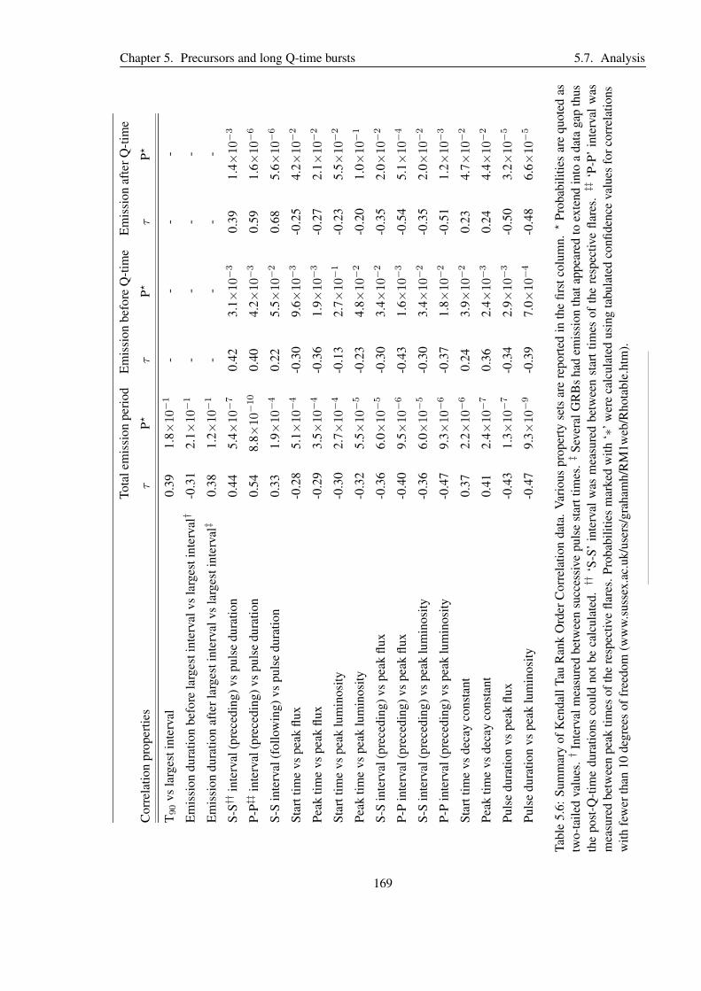
Chapter 5. Precursors and long Q-time bursts 5.7. Analysis
TotalemissionperiodEmissionbeforeQ-timeEmissionafterQ-time
Correlationproperties
τP
?τ
P?
τP
?
T90vslargestinterval
0.39
1.8×
10−
1-
--
-
Emissiondurationbeforelargestintervalvslargestinterval
†-0.31
2.1×
10−
1-
--
-
Emissiondurationafterlargestintervalvslargestinterval
‡0.38
1.2×
10−
1-
--
-
S-S
††interval(preceding)vspulseduration
0.44
5.4×
10−
70.42
3.1×
10−
30.39
1.4×
10−
3
P-P
‡‡interval(preceding)vspulseduration
0.54
8.8×
10−
10
0.40
4.2×
10−
30.59
1.6×
10−
6
S-Sinterval(following)vspulseduration
0.33
1.9×
10−
40.22
5.5×
10−
20.68
5.6×
10−
6
Starttimevspeakflux
-0.28
5.1×
10−
4-0.30
9.6×
10−
3-0.25
4.2×
10−
2
Peaktimevspeakflux
-0.29
3.5×
10−
4-0.36
1.9×
10−
3-0.27
2.1×
10−
2
Starttimevspeakluminosity
-0.30
2.7×
10−
4-0.13
2.7×
10−
1-0.23
5.5×
10−
2
Peaktimevspeakluminosity
-0.32
5.5×
10−
5-0.23
4.8×
10−
2-0.20
1.0×
10−
1
S-Sinterval(preceding)vspeakflux
-0.36
6.0×
10−
5-0.30
3.4×
10−
2-0.35
2.0×
10−
2
P-Pinterval(preceding)vspeakflux
-0.40
9.5×
10−
6-0.43
1.6×
10−
3-0.54
5.1×
10−
4
S-Sinterval(preceding)vspeakluminosity
-0.36
6.0×
10−
5-0.30
3.4×
10−
2-0.35
2.0×
10−
2
P-Pinterval(preceding)vspeakluminosity
-0.47
9.3×
10−
6-0.37
1.8×
10−
2-0.51
1.2×
10−
3
Starttimevsdecayconstant
0.37
2.2×
10−
60.24
3.9×
10−
20.23
4.7×
10−
2
Peaktimevsdecayconstant
0.41
2.4×
10−
70.36
2.4×
10−
30.24
4.4×
10−
2
Pulsedurationvspeakflux
-0.43
1.3×
10−
7-0.34
2.9×
10−
3-0.50
3.2×
10−
5
Pulsedurationvspeakluminosity
-0.47
9.3×
10−
9-0.39
7.0×
10−
4-0.48
6.6×
10−
5
Table5.6:SummaryofKendallTauRankOrderCorrelationdata.Variouspropertysetsarereportedinthefirstcolumn.
?Probabilitiesarequotedas
two-tailedvalues.†Intervalmeasuredbetweensuccessivepulsestarttimes.‡SeveralGRBshademissionthatappearedtoextendintoadatagapthus
thepost-Q-timedurationscouldnotbecalculated.
††‘S-S’intervalwasmeasuredbetweenstarttimesoftherespectiveflares.
‡‡‘P-P’intervalwas
measuredbetweenpeaktimesoftherespectiveflares.Probabilitiesmarkedwith‘∗’werecalculatedusingtabulatedconfidencevaluesforcorrelations
withfewerthan10degreesoffreedom(www.sussex.ac.uk/users/grahamh/RM1web/Rhotable.htm).
169

Chapter 5. Precursors and long Q-time bursts 5.7. Analysis
(a) Reproduction of Chincarini et al. (2007) figure 12 showing the distri-
bution of the ratio of peak intensities between two successive events: X-
ray flares (solid red line, 68 flares), γ-ray pulses (dashed green line, 46
pulses) and the combined sample (dotted blue line, 104 pulses). This distri-
bution was fit with a Gaussian function giving <log(peaki+1/peaki) >=
−0.157 and σlog = 0.41, provided two outlying points are ignored (see § 5
C07).
(b) Cumulative frequency plot using pulse values from this study
(73 pulses). Applying a Gaussian function to this distribution gives
<log(peaki+1/peaki) >= 5 × 10⁻⁴ and σlog = 0.45.
Figure 5.5: Comparison plots displaying the distribution of the ratio between the peaks of two succes-
sive pulses from C07 and this study.
170

Chapter 5. Precursors and long Q-time bursts 5.7. Analysis
Three of the ten GRBs used in Lazzati et al. (2008) are included in the sample used in this work (GRB
050820A, 060115 and 060124).
The average flare luminosity in Lazzati’s work was calculated using the following formula (their equa-
tion 1):
< L >t1,t2=1
nGRB
nf∑
i=1
Liδti,1,2, (5.2)
where Li is the average luminosity of the ith flare during its active time, nGRB = 11 is the total
number of GRBs considered in this work, nf = 73 is the total number of flares and 0 ≤ δti,1,2 ≤ 1 is
the fraction of the time in the interval (t1, t2) during which the ith is active. Following the method of
Lazzati et al. (2008) this prescription is equivalent to the assumption that the flares have a square shape.
The authors argued that when both a Gaussian and triangular profile were used the resultant values
for the average luminosity were consistent with the simplified approximation, within the error limits.
Whilst not being a realistic approximation to the temporal characteristics of typical GRB flares/pulses
this prescription has been retained in this analysis so that the results obtained are directly comparable
to those obtained by Lazzati et al. (2008).
Figure 1 of Lazzati et al. (2008) is reproduced in figure 5.6(a), whilst the results from the pulses in this
study are shown in figure 5.6(b). Attempting a power law fit to the data in figure 5.6(b) produced an
index of −0.37+0.10−0.09, which gave an extremely poor χ
2 fit; nor was it consistent with the value found
by Lazzati et al. (2008). Fixing the decay index at −1.5 worsened the fit further. However, it should
be noted that the results of this work cover a much shorter time span than that covered by Lazzati et al.
(2008). If the first three points of figure 5.6(a) are considered on their own (time < 200 s) then the
power law index would be somewhat shallower than −1.5, perhaps indicating that there is a slightly
different average pulse luminosity behaviour at early times. However, given the small sample numbers
in both works it is difficult to ascertain whether this is a real trend or not.
Lazzati et al. (2008) also convert their average flare luminosity values into equivalent accretion rates (in
solar masses s−1, their figure 3), assuming that: the GRB jet is beamed into 1% of the sky; and there was
an efficiency of 0.1% when the accretion rate was converted to jet luminosity. All of their data points
lie below the level at which the material surrounding the central BH switches from a neutrino-cooled to
171
Chapter 5. Precursors and long Q-time bursts 5.7. Analysis
an advective disk. This occurs at ∼ 10−3 − 10−2M¯s−1 depending on the viscosity prescription used
(Chen & Beloborodov, 2007). On the same figure they also show the average accretion rate during
the prompt phase to be above this switch threshold. However, as can be seen from a comparison of
figure 5.6(a) and 5.6(b), the early time, average flare luminosities calculated from my study (i.e. a
measurement of this prompt phase) are at a comparable absolute value to Lazzati’s earliest data points.
Conducting a similar conversion to accretion rate using the same assumptions would not place my data
points above the switching threshold.
5.7.6 Underlying afterglow behaviour
Whilst collating the flux light curves it was noted that there appeared to be strong similarities between
the late-time afterglow behaviour and absolute flux values for several GRBs in the sample. Given the
limited number of GRBs considered by this study such similarities could be entirely spurious. However,
with that caveat in mind, the light curves were separated into four groups:
• Group 1: 050319, 060714A, 060904B, see figure 5.7(a).
– Fluxave.(1 ks) ∼ 1 × 10⁻¹¹ ergs cm−2 s−1. At that time the afterglow exhibits phase II
decay with αave ∼ 0.39.
– Fluxave.(40 ks) ∼ 2 × 10⁻¹³ ergs cm−2 s−1. At that time the afterglow exhibits phase III
decay with αave ∼ 1.37.
• Group 2: 050820A, 060124, 061121, see figure 5.7(c).
– Fluxave.(1 ks) ∼ 2 × 10⁻¹⁰ ergs cm−2 s−1. At that time the afterglow appears to be at the
end of phase II decay with α ∼ave 0.26.
– Fluxave.(40 ks) ∼ 2 × 10⁻¹² ergs cm−2 s−1. At that time the afterglow exhibits phase III
decay with αave ∼ 1.29.
• Group 3: 060115, 060526, see figure 5.7(e).
– Fluxave.(1 ks) ∼ 4 × 10⁻¹² ergs cm−2 s−1. At that time the afterglow exhibits phase II
decay with αave ∼ 0.49.
172
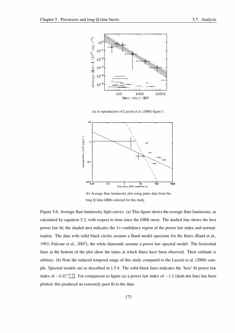
Chapter 5. Precursors and long Q-time bursts 5.7. Analysis
(a) A reproduction of Lazzati et al. (2008) figure 1.
0.01 0.1 1 10 100 10000.01
0.1
1
10
Ave
rag
e f
lare
L (
x1
050 e
rgs s
−1)
Time since GRB, restframe (s)0.01 0.1 1 10 100 1000
0.01
0.1
1
10
(b) Average flare luminosity plot using pulse data from the
long Q-time GRBs selected for this study.
Figure 5.6: Average flare luminosity light curves. (a) This figure shows the average flare luminosity, as
calculated by equation 5.2, with respect to time since the GRB onset. The dashed line shows the best
power law fit; the shaded area indicates the 1σ confidence region of the power law index and normal-
isation. The data with solid black circles assume a Band model spectrum for the flares (Band et al.,
1993; Falcone et al., 2007); the white diamonds assume a power law spectral model. The horizontal
lines at the bottom of the plot show the times at which flares have been observed. Their ordinate is
arbitary. (b) Note the reduced temporal range of this study compared to the Lazzati et al. (2008) sam-
ple. Spectral models are as described in § 5.4. The solid black lines indicates the ‘best’ fit power law
index of −0.37+0.10−0.09. For comparison to figure (a) a power law index of −1.5 (dash-dot line) has been
plotted; this produced an extremely poor fit to the data.
173
Chapter 5. Precursors and long Q-time bursts 5.7. Analysis
– Fluxave.(40 ks) ∼ 1 × 10⁻¹³ ergs cm−2 s−1. At that time the afterglow exhibits phase III
decay with αave ∼ 1.50.
• Group 4: 060210, 060418, 060607A, see figure 5.7(g).
– Fluxave.(1 ks) ∼ 5 × 10⁻¹¹ ergs cm−2 s−1. At that time the afterglow exhibits phase II
decay with αave ∼ 1.11.
– Fluxave.(40 ks) has a wide dispersion from ∼ 4 × 10⁻¹⁴ to ∼ 1 × 10⁻¹² ergs cm−2 s−1.
At that time the afterglow also exhibits a wide dispersion with a decay index between 1.50
and 3.24.
It is interesting to note that despite the differences in the late-time afterglow behaviour all groups appear
to have a break between phase II and III at ∼ 5 ks.
Previously Boer & Gendre (2000), Gendre & Boer (2005) and Gendre et al. (2008) proposed that there
are several subclasses of GRB afterglow behaviour, dependant in their X-ray and optical behaviour.
Focussing only on the X-ray behaviour Gendre et al. (2008) separates these into group I and II bursts,
which have average fluxes of∼ 7.0×10⁻¹² ergs cm−2 s−1 and 3.1×10⁻¹³ ergs cm−2 s−1 respectively
at 1 day in the observer’s reference frame assuming an average redshift of 1 (equivalent to 40 ks in the
burst’s rest frame). The classes proposed above broadly fit in with Gendre & Boer’s (2008) classifica-
tion: the flux of group 2 bursts have the same order of magnitude flux as group I at 40 ks, whilst the flux
of group 1 and 3 is approximately the same as Gendre & Boer’s (2008) group II. The fluxes of group 4
bursts at 40 ks are widely distributed so it is not possible to constrain, with this sample number, which
subclass they belong to.
The same groupings were retained for the composite plots of the GRB luminosity light curves (figures
5.7 b, d, f and h) to see if the afterglow behaviour remained closely related. Whilst the absolute shape
of the late-time afterglows remained the same, the luminosities were markedly different. In the future
the analysis of more long Q-time bursts with known redshifts would confirm whether these are distinct
afterglow subclasses, but for the time being no firm conclusions can be drawn.
Decay indices and break times of the underlying afterglow behaviours for this sample are reported in
table 5.7 (assuming sharply broken power law segments); GRBs are collated into the groups stated
above to illustrate the similarity of their late-time afterglow behaviour and to make it easier to compare
174

Chapter 5. Precursors and long Q-time bursts 5.7. Analysis
0.01 0.1 1 10 100 1000 104 105 10610−14
10−13
10−12
10−11
10−10
10−9
10−8
10−7
10−6
Flu
x (
erg
s c
m−
2 s
−1)
Time, restframe (s)
(a) Group 1: GRB 050319 (black), GRB
060714A (red) and GRB 060904B (green)
0.01 0.1 1 10 100 1000 104 105 1061000
104
105
106
107
108
109
1010
1011
1012
1013
Lum
inosity (
x10
40 e
rgs s
−1)
Time, restframe (s)
(b) Group 1: GRB 050319 (black), GRB
060714A (red) and GRB 060904B (green)
0.01 0.1 1 10 100 1000 104 105 10610−14
10−13
10−12
10−11
10−10
10−9
10−8
10−7
10−6
Flu
x (
erg
s c
m−
2 s
−1)
Time, restframe (s)
(c) Group 2: GRB 050820A (black), GRB
060124 (red) and GRB 061121 (green)
0.01 0.1 1 10 100 1000 104 105 1061000
104
105
106
107
108
109
1010
1011
1012
1013
Lum
inosity (
x10
40 e
rgs s
−1)
Time, restframe (s)
(d) Group 2: GRB 050820A (black), GRB
060124 (red) and GRB 061121 (green)
0.01 0.1 1 10 100 1000 104 105 10610−14
10−13
10−12
10−11
10−10
10−9
10−8
10−7
10−6
Flu
x (
erg
s c
m−
2 s
−1)
Time, restframe (s)
(e) Group 3: GRB 060115 (black), GRB
060526 (red)
0.01 0.1 1 10 100 1000 104 105 1061000
104
105
106
107
108
109
1010
1011
1012
1013
Lum
inosity (
x10
40 e
rgs s
−1)
Time, restframe (s)
(f) Group 3: GRB 060115 (black), GRB
060526 (red)
0.01 0.1 1 10 100 1000 104 105 10610−14
10−13
10−12
10−11
10−10
10−9
10−8
10−7
10−6
Flu
x (
erg
s c
m−
2 s
−1)
Time, restframe (s)
(g) Group 4: GRB 060210 (black), GRB
060418 (red) and GRB 060607A (green)
0.01 0.1 1 10 100 1000 104 105 1061000
104
105
106
107
108
109
1010
1011
1012
1013
Lum
inosity (
x10
40 e
rgs s
−1)
Time, restframe (s)
(h) Group 4: GRB 060210 (black), GRB
060418 (red) and GRB 060607A (green)
Figure 5.7: Flux light curve (1-20 keV) in the rest frame of the burst, compared to luminosity light
curves (over the same energy range).
175
Chapter 5. Precursors and long Q-time bursts 5.7. Analysis
their early time behaviour. As stated in § 5.6 smoothly broken power law models were also applied to
selected portions of the late-time afterglows, the results of which are reported in table 5.8.
The general behaviour of the majority of the light curves modelled in this sample is that of the canonical
light curve described in § 1.3.3, plus a power law afterglow contribution to the phase 0 emission (in
addition to the typical pulse behaviour). It should be noted that there are gaps in the model parameters
reported in table 5.7; these were either due to periods when the GRB light curves were poorly/not
sampled or as result of multiple, overlapping pulses obscuring the underlying behaviour and preventing
well constrained, ‘stable’34 fits with multiple breaks from being carried out. In such cases a model
containing the maximum number of expected breaks did not produce well constrained values, therefore
a model with fewer breaks had to be utilised. As a result the phase I decay portion of the canonical
light curve may have been present but could not be modelled as it appeared to have been obscured by a
contemporaneous pulse; for example GRB 060714A and GRB 060904B.
GRBs included in the fourth ‘group’ (060210, 060418 and 060607A) appeared to be markedly dif-
ferent from the other bursts included in this sample; nor do they appear to reflect canonical afterglow
behaviour. They potentially belong to a subset of bursts that do not show a ‘normal’ plateau phase but
instead decay rapidly.
5.7.7 Phase 0 emission: Prompt power laws
Phase 0 emission appears to be typified by an underlying power law with a decay index of∼ 0.5, which
is strikingly similar to that seen during canonical phase II decay. The decay indices of the two phases
in question are plotted in figure 5.7; this plot seems to indicate that there may be an anti-correlation
between the two values. A Spearman Rank test gave rs = −0.71 for a total of 7 degrees of freedom.
Tabulated confidence values35 for correlations with fewer than 10 degrees of freedom indicated that the
apparent negative correlation was not significant at the 95% confidence level. The same relationship
was analysed using the Kendall tau coefficient giving τ = −0.62 (P= 0.07) also indicating that the
apparent anti-correlation was not significant given the available data.
34A ‘stable’ model fit is, as expected, defined as one where the parameter values do not change if a fit or error
command was issued once best efforts had been made to find the global minimum fit.35www.sussex.ac.uk/users/grahamh/RM1web/Rhotable.htm
176

Chapter 5. Precursors and long Q-time bursts 5.7. Analysis
GroupGRB
Phase0
Break
1PhaseI
Break
2PhaseII
Break
3PhaseIII
Break
4PhaseIV
†
decayindex
(s)
decayindex
(s)
decayindex
(ks)
decayindex
(ks)
decayindex
050319
0.65
+0.0
9−
0.0
966
+10
−11
3.76
+0.8
4−
0.8
713
3+13
−9
0.49
+0.0
4−
0.0
37.
38+
1.6
4−
0.8
41.
47+
0.0
4−
0.1
0-
-
1060714A
0.87
+0.2
6−
0.0
7-
-11
1+84
−104
0.29
+0.1
7−
0.2
11.
25+
0.5
4−
0.4
21.
23+
0.0
6−
0.0
6-
-
060904B
0.86
+0.0
3−
0.0
3-
--
-3.
98+
1.4
3−
1.6
01.
41+
0.1
1−
0.1
2-
-
050820A
0.11
+0.3
1−
0.2
24+
4−
22.
07+
0.2
2−
0.2
5‡
‡‡
1.24
+0.0
4−
0.0
318
8+106
−73
1.74
+0.2
3−
0.1
9
2060124
--
1.30
+0.0
9−
0.1
836
+5
−14
0.24
+0.0
2−
0.0
65.
43+
0.3
0−
0.3
41.
31+
0.0
3−
0.0
334
5+35
−205
2.09
+1.1
6−
0.7
8
061121
0.41
+0.0
4−
0.0
51+
1−
11.
68+
0.0
3−
0.0
211
+1
−1
0.28
+0.0
4−
0.0
51.
64+
0.1
8−
0.1
51.
33+
0.0
1−
0.0
2-
-
3060115
0.22
+0.0
6−
0.0
928
+3
−6
2.48
+0.5
9−
0.1
821
0+35
−66
0.71
+0.1
0−
0.1
29.
07+
10.4
4−
4.4
71.
24+
0.5
1−
0.2
4-
-
060526
0.91
+0.0
4−
0.0
613
9+42
−17
2.32
+1.4
2−
0.5
027
6+66
−59
0.26
+0.1
8−
0.1
64.
87+
1.8
4−
1.4
51.
73+
0.2
6−
0.2
3-
-
060210
0.50
+0.0
3−
0.0
4-
-12
10+
230
−270
0.98
+0.0
7−
0.0
75.
85+
0.6
9−
0.6
01.
42+
0.0
6−
0.0
6-
-
4060418
0.10
+0.1
1−
0.1
5-
-16
+5
−3
1.23
+0.0
3−
0.0
33.
75+
5.2
1−
1.9
91.
58+
0.2
2−
0.1
2-
-
060607A
0.39
+0.0
2−
0.0
2-
--
-3.
06+
0.0
9−
0.0
9-
-3.
24+
0.1
3−
0.1
3
Table5.7:SummaryofGRBrestframelightcurvepropertiesassumingsharplybrokenpowerlawsegments.Allvaluesarereportedintherestframe
oftheburst.
T0istakentobethepeakoffirstemissionpulse(SNR=3).†ThetemporalplacementofthisdecaysegmentisconsistentwithphaseIV
butitmaynotreflectthephysicalpropertiesexpectedfromcanonicalphaseIVdecay.‡DuetothebreakinobservationsofGRB050820Aitwasnot
possibletoconstrainanydecayslopesorbreaksbetween∼80-1280s.
177

Chapter 5. Precursors and long Q-time bursts 5.7. Analysis
GRB Best fit parameters for a smoothly broken power law
α1 α2 break time (s) χ2/ν smoothing
050319 0.40+0.08−0.15 2.24+0.36
−0.21 21300+7890−5860 106/131 −0.63+0.12
−0.20
060714A 0.33+0.14−0.20 1.22+0.07
−0.06 1320+370−380 56/51 −12.6+0.08
−0.11
060904B < 0.35 1.41+0.35−0.04 1040+12000
−630 32/50 −1 (f)
050820A 1.12+0.03−0.03 1.74+0.12
−0.09 129000+6660−6620 137/140 −1 (f)
060124 0.71+0.07−0.10 1.43+0.04
−0.02 4900+200−200 350/285 −1 (f)
061121 0.25+0.06−0.06 1.49+0.04
−0.04 2600+750−550 292/321 −1 (f)
060115†
060526 0.29+0.14−0.16 1.95+0.36
−0.30 6710+4690−3030 24/28 −1 (f)
060210 0.26+0.32−0.44 1.45+0.14
−0.09 1820+2350−710 261/246 −1 (f)
060418 1.04+0.04−0.03 1.75+0.11
−0.10 3730+1380−850 154/136 −1 (f)
060607A 0.40+0.04−0.04 3.90+0.24
−0.21 3650+210−210 294/203 −1 (f)
Table 5.8: Summary of ‘afterglow’ light curve fits using a smoothly broken power law model, where
T0 is taken to be the peak of first emission pulse (SNR = 3). These fits only include data after phase I
emission or the end of the last decay portion of a late time flare. All break time values are in the rest
frame of the burst. Smoothing values followed by (f) indicate that the smoothing parameter has been
frozen at the standard value of -1 (see discussion in § 2.2.1 of this thesis). †GRB 060115: a smoothly
broken power law model gives very poorly constrained parameters.
178

Chapter 5. Precursors and long Q-time bursts 5.7. Analysis
0 0.2 0.4 0.6 0.8 1 1.2
00
.51
Ph
ase
II
em
issio
n:
de
ca
y in
de
x
Phase 0 emission: decay index
Figure 5.8: Phase 0 decay index plotted versus phase II decay index, plotted from data in table 5.7.
It is possible that the phase 0 power law values measured here may be indicative of a period of energy
injection akin to the standard explanation for phase II emission. Thus phase 0 emission potentially
originates from the first series of pulses/ the ‘precursor’ whilst phase II potentially originates from the
pulses that occur after the Q-time. See further discussion in § 5.7.9.
GRB 060124 was the only GRB in the sample without a measured phase 0 decay index. I attempted
a further fit with a model comprising of five power law segments (sharply broken) and sixteen pulses,
however, this model proved to be more complex than QDP could handle. Instead a different four power
law/ sixteen pulse model was applied, this time attempting to find a phase 0 decay index at the expense
of the phase ‘IV’ index. This produced a statistically comparable fit with intermediate (phase I to III)
decay indices and break times that were consistent with those reported in table 5.7. However, the phase
0 decay index of this fit was not well constrained, αphase 0 < 0.50, with a break seen at 5+1−1 s. This
would be consistent with the trend noted above, given the measured phase II decay index of 0.24+0.02−0.06,
if the decay index was near the upper limit given.
179
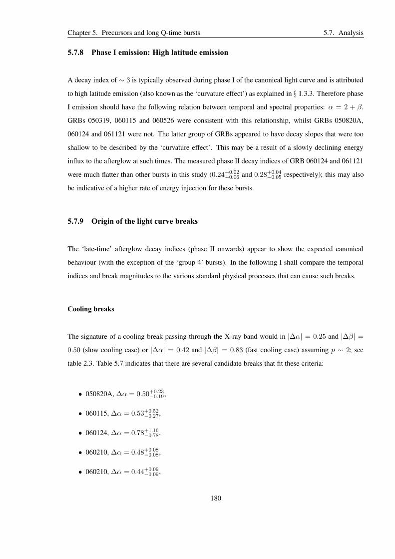
Chapter 5. Precursors and long Q-time bursts 5.7. Analysis
5.7.8 Phase I emission: High latitude emission
A decay index of ∼ 3 is typically observed during phase I of the canonical light curve and is attributed
to high latitude emission (also known as the ‘curvature effect’) as explained in § 1.3.3. Therefore phase
I emission should have the following relation between temporal and spectral properties: α = 2 + β.
GRBs 050319, 060115 and 060526 were consistent with this relationship, whilst GRBs 050820A,
060124 and 061121 were not. The latter group of GRBs appeared to have decay slopes that were too
shallow to be described by the ‘curvature effect’. This may be a result of a slowly declining energy
influx to the afterglow at such times. The measured phase II decay indices of GRB 060124 and 061121
were much flatter than other bursts in this study (0.24+0.02−0.06 and 0.28+0.04
−0.05 respectively); this may also
be indicative of a higher rate of energy injection for these bursts.
5.7.9 Origin of the light curve breaks
The ‘late-time’ afterglow decay indices (phase II onwards) appear to show the expected canonical
behaviour (with the exception of the ‘group 4’ bursts). In the following I shall compare the temporal
indices and break magnitudes to the various standard physical processes that can cause such breaks.
Cooling breaks
The signature of a cooling break passing through the X-ray band would in |∆α| = 0.25 and |∆β| =
0.50 (slow cooling case) or |∆α| = 0.42 and |∆β| = 0.83 (fast cooling case) assuming p ∼ 2; see
table 2.3. Table 5.7 indicates that there are several candidate breaks that fit these criteria:
• 050820A, ∆α = 0.50+0.23−0.19,
• 060115, ∆α = 0.53+0.52−0.27,
• 060124, ∆α = 0.78+1.16−0.78,
• 060210, ∆α = 0.48+0.08−0.08,
• 060210, ∆α = 0.44+0.09−0.09,
180

Chapter 5. Precursors and long Q-time bursts 5.7. Analysis
• 060418, ∆α = 0.35+0.22−0.12.
However, none of these breaks show any definite signs of spectral change either from the spectra at the
break time or hardness ratio (HR) plots at the same time (if spectra are not available due to low counts;
see Appendix 5.A). GRB 050820A potentially shows a change in spectral properties from the HR plot
but the spectra at this time are consistent with an unchanging photon index of ∼ 2. Thus I rule out
cooling breaks as an origin for any of the breaks measured in this analysis.
Jet breaks
The signatures of a jet break are: ∆α = 1.0, no spectral variation across the break and the post-
break decay index should be equal to the electron spectral index, p (as long as p > 2, otherwise a
different α − p relation should be adopted; Zhang & Meszaros 2004; Dai & Cheng 2001). There were
several candidate bursts with temporal breaks consistent with the expected value (see table 5.9). Only
one break, the second (downwards) sharp break in the afterglow of GRB 060124, was consistent with
∆α = 1.0 and αpost break = p. In this case it was not possible to distinguish between the two emission
scenarios, i.e. ν > νc or ν < νc.
End of energy injection
A break is expected to be present between canonical phase II and III decay as a result of the end of
energy injection from the central engine, see § 1.3.3; such breaks should show little or no spectral
evolution. Using the equations detailed in § 1.3.3 I have calculated the expected post-break decay
indices from the measured spectral parameters for a variety of ν relations and circumburst densities for
the scenario whereby energy injection is moderated by ejecta with a wide Lorentz factor distribution.
The corresponding power law indices s (E(> Γ) ∝ Γ1−s, s > 1 for significant energy injection) and a
(E(t > ti) ∝ ta) were also calculated.
Given the similarity of the measured values for phase 0 and phase II decay indices (§ 5.7.7) it is possible
that the underlying phase 0 emission was a result of the same energy injection process. Therefore
calculations were carried out to assess whether any of the breaks between phase 0 and phase I would fit
181

Chapter 5. Precursors and long Q-time bursts 5.7. Analysis
GRB ∆α β αpost break p† αpost break
(ν > νc) (ν < νc) consistent with p?
050319 0.98+0.06−0.10 1.07+0.17
−0.17 1.47+0.04−0.10 2.14+0.34
−0.34 3.14+0.34−0.34 Not consistent
060714 0.94+0.18−0.22 0.98+0.19
−0.19 1.23+0.06−0.06 1.96+0.38
−0.38 2.96+0.38−0.38 Not consistent
060124 1.07+0.04−0.07 0.88+0.20
−0.13 1.31+0.03−0.03 1.76+0.40
−0.26 2.76+0.40−0.26 Not consistent
060124 0.78+1.16−0.78 0.98+0.11
−0.11 2.09+1.16−0.78 1.96+0.40
−0.26 2.96+0.40−0.26 Both consistent
061121 1.05+0.04−0.05 1.01+0.12
−0.12 1.33+0.01−0.03 2.02+0.24
−0.24 3.01+0.24−0.24 Not consistent
Table 5.9: Summary of jet break candidates. Only the second (downwards) sharp break in GRB 060124
is consistent with a jet break. † These values were calculated using the observed value of β (3rd column)
and the relationship between p and β for afterglow models during the jet phase, for the case where
ν > νc and ν < νc, as given by table 1 of Zhang & Meszaros (2004) (and references therein) assuming
p > 2.
with this hypothesis for the model where energy injection is moderated by ejecta with a wide Lorentz
factor distribution; the results are reported in table 5.10. No combination of parameters produced an
acceptable fit to the phase 0 to phase I decay for GRB 060115 or GRB 060526. The remaining GRBs
(050319, 050820A and 061121) indicated that scenarios where ν > νm were favoured, however, there
was no clear trend to indicate a favoured circumburst environment. These results, combined with the
measured magnitude of the decay indices, indicates that the underlying behaviour of phase 0 may be
related to energy injection.
Table 5.11 reports the allowed conditions for the breaks seen between phase II and phase III for the
same model. Similarly to the phase 0 to phase I transition examples discussed above the scenario
where ν > νm was favoured in the majority of cases for the measured phase II to phase III break.
There appeared to be no consistent trend for the circumburst environment, though two cases (GRB
050319 and 061121) could only be fit by a model with νm < ν < νc and k = 0. Interestingly no
combination of parameters were able to fit the breaks in GRB 060526, indicating that neither break can
be explained by energy injection from ejecta with a wide Lorentz factor distribution.
The scenario wherein long term central engine activity provides the source of energy injection was
182
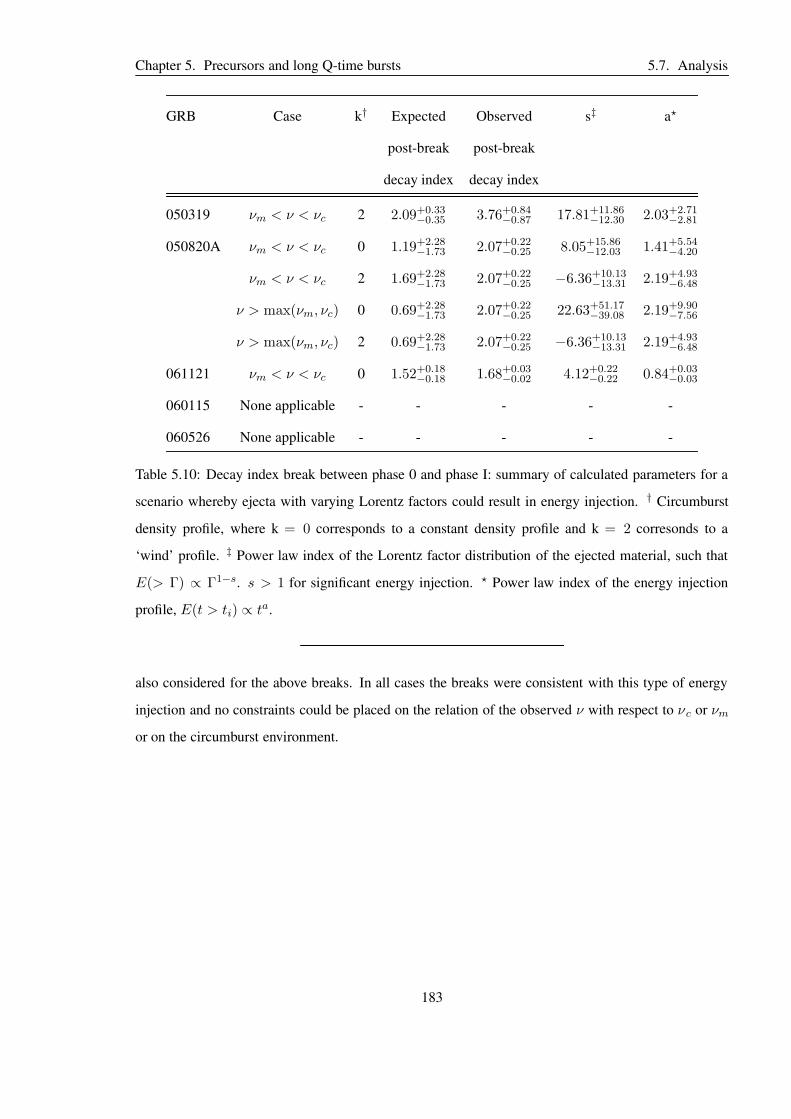
Chapter 5. Precursors and long Q-time bursts 5.7. Analysis
GRB Case k† Expected Observed s‡ a?
post-break post-break
decay index decay index
050319 νm < ν < νc 2 2.09+0.33−0.35 3.76+0.84
−0.87 17.81+11.86−12.30 2.03+2.71
−2.81
050820A νm < ν < νc 0 1.19+2.28−1.73 2.07+0.22
−0.25 8.05+15.86−12.03 1.41+5.54
−4.20
νm < ν < νc 2 1.69+2.28−1.73 2.07+0.22
−0.25 −6.36+10.13−13.31 2.19+4.93
−6.48
ν > max(νm, νc) 0 0.69+2.28−1.73 2.07+0.22
−0.25 22.63+51.17−39.08 2.19+9.90
−7.56
ν > max(νm, νc) 2 0.69+2.28−1.73 2.07+0.22
−0.25 −6.36+10.13−13.31 2.19+4.93
−6.48
061121 νm < ν < νc 0 1.52+0.18−0.18 1.68+0.03
−0.02 4.12+0.22−0.22 0.84+0.03
−0.03
060115 None applicable - - - - -
060526 None applicable - - - - -
Table 5.10: Decay index break between phase 0 and phase I: summary of calculated parameters for a
scenario whereby ejecta with varying Lorentz factors could result in energy injection. † Circumburst
density profile, where k = 0 corresponds to a constant density profile and k = 2 corresonds to a
‘wind’ profile. ‡ Power law index of the Lorentz factor distribution of the ejected material, such that
E(> Γ) ∝ Γ1−s. s > 1 for significant energy injection. ? Power law index of the energy injection
profile, E(t > ti) ∝ ta.
also considered for the above breaks. In all cases the breaks were consistent with this type of energy
injection and no constraints could be placed on the relation of the observed ν with respect to νc or νm
or on the circumburst environment.
183

Chapter 5. Precursors and long Q-time bursts 5.7. Analysis
GRB Case k† Expected Observed s‡ a?
post-break post-break
decay index decay index
050319 νm < ν < νc 0 1.61+0.26−0.26 1.47+0.04
−0.10 3.16+0.55−0.61 0.64+0.22
−0.25
060714A νm < ν < νc 0 1.47+0.29−0.29 1.23+0.06
−0.06 3.13+0.870.97 0.63+0.35
−0.39
ν > max(νm, νc) 0 0.97+0.29−0.29 1.23+0.06
−0.06 4.70+1.37−1.53 0.95+0.55
−0.62
ν > max(νm, νc) 2 0.97+0.29−0.29 1.23+0.06
−0.06 76.20+310.88−365.94 0.95+5.48
−6.45
060124 νm < ν < νc 0 1.55+0.33−0.29 1.31+0.03
−0.03 3.46+0.78−0.69 0.71+0.31
−0.28
ν > max(νm, νc) 0 1.05+0.33−0.20 1.31+0.03
−0.03 5.33+1.20−1.09 1.05+0.47
−0.43
ν > max(νm, νc) 2 1.05+0.33−0.20 1.31+0.03
−0.03 −76.82+165.50−164.33 1.05+3.21
−3.19
061121 νm < ν < νc 0 1.52+0.18−0.18 1.33+0.01
−0.02 3.41+0.17−0.17 0.69+0.02
−0.02
060115 ν > max(νm, νc) 0 1.18+0.15−0.14 1.24+0.51
−0.24 2.60+2.61−1.37 0.50+1.00
−0.53
ν > max(νm, νc) 2 1.18+0.15−0.14 1.24+0.51
−0.24 5.00+6.97−3.65 0.50+0.99
−0.52
060526 None applicable - - - - -
060210 ν > max(νm, νc) 0 1.45+0.36−0.33 1.42+0.06
−0.06 2.17+0.61−0.58 0.38+0.22
−0.20
ν > max(νm, νc) 2 1.45+0.36−0.33 1.42+0.06
−0.06 3.48+1.21−1.16 0.38+0.19
−0.18
060418 νm < ν < νc 0 1.53+0.41−0.38 1.58+0.22
−0.12 1.67+1.14−0.38 0.23+0.32
−0.20
νm < ν < νc 2 2.03+0.41−0.38 1.58+0.22
−0.12 3.12+2.45−1.55 0.35+0.38
−0.24
Table 5.11: Decay index break between phase II and phase III: summary of calculated parameters for
a scenario whereby ejecta with varying Lorentz factors could result in energy injection. † Circumburst
density profile, where k = 0 corresponds to a constant density profile and k = 2 corresonds to a
‘wind’ profile. ‡ Power law index of the Lorentz factor distribution of the ejected material, such that
E(> Γ) ∝ Γ1−s. s > 1 for significant energy injection. ? Power law index of the energy injection
profile, E(t > ti) ∝ ta.
184

Chapter 5. Precursors and long Q-time bursts 5.8. Conclusions
5.8 Conclusions
It has long been hypothesised (Colgate, 1973, 1974) that phase 0 GRB emission is preceded by a
transient signal with a different physical origin, and therefore spectral properties, to the rest of the
burst. Current theoretical models propose that ‘precursors’ are subdivided into two classes: fireball and
progenitor precursors (§5.1). Both are thought to generate thermal signals, however, these may be up-
scattered to produce non-thermal spectra or be obscured by non-thermal radiation emitted at the same
time. Definitions of such precursor emission vary greatly between different studies in the literature
and often depend on the observed energy range and instrument used. One particular ambiguity in the
models proposed so far is the delay between the precursor and phase 0 emission; times range between
little as 10 s (Wang & Meszaros, 2007) up to several 100 s (Koshut et al., 1995; Lazzati, 2005).
A separate study conducted by Nakar & Piran (2002) indicated that there are unusually long intervals
of little or no emission during phase 0 that they call quiescent times (Q-times, §5.1.3). They stress
that such periods are not the same as the delays between precursor and phase 0 emission reported by
Koshut et al. (1995), however, it is interesting to note that the timescales discussed in both works bear
a striking resemblance. Such quiescent periods indicate that there is a change in central engine activity
during these times. Given the increasing evidence that phase 0 and phase V emission share a common
origin (internal shocks) there is a possibility that precursors are merely another aspect of this emission.
Rather than adopt fully instrumentally based criteria (i.e. emission occurring before a burst ‘trigger’
etc) in this study I chose to select GRBs with long quiescent, since quiescent periods indicate a change
in central engine activity, which is the essence of the definition of a precursor. Studying bursts with long
Q-times may help to distinguish whether their early time emission (i.e. whether they show evidence
for precursor emission as discussed in the literature), pulse properties as a whole or their long term
afterglows are different to those of other GRBs. In this work I have taken a subsection of Swift GRBs
with long Q-times (> 50 s in the observer’s reference frame) and known redshifts (with a range be-
tween 0.703 and 3.910) to produce a series of joint BAT-XRT flux and luminosity light curves covering
a rest frame energy range of 1 − 20 keV. Pulse spectral, temporal and energetic properties were ex-
tracted from these light curves. No strong evidence was found to suggest that the precursors/early time
emission pulses in this sample were spectrally different to the rest of the main emission period over
the energy ranges observed by BAT. Pulse properties were used to calculate a series of Spearman Rank
185

Chapter 5. Precursors and long Q-time bursts 5.8. Conclusions
and Kendall Tau correlations. Several correlations and anti-correlations were found in the pulse tem-
poral and energetic properties that indicated a common origin for all pulses (as suggested by previous
studies), irrespective of which instrument or energy range they are typically observed in.
This study has reaffirmed that, at the current stage of theoretical understanding, constructing a defini-
tion for precursor events is as important as studying them. Furthermore it has provided evidence for
extending the link between phase 0 emission and flares to events that were previously designated as
precursors. Potentially all of these seemingly separate events may share a common origin. The corre-
lations between pulse properties noted were all consistent with the accretion models proposed by Perna
et al. (2006, delayed accretion from a fragmented disk) and Proga & Zhang (2006, accretion moderated
by a magnetic barrier). I was not able to confirm the average pulse luminosity light curve as proposed
by Lazzati et al. (2008).
Additionally the underlying afterglows of this subset of bursts were modelled; all of which were consis-
tent with the canonical GRB light curve model. A similarity was noted between the underlying phase
0 and phase II decay indices hinting at a common origin for both. My analysis showed that both decay
indices were consistent with existing energy injection models.
186

Chapter 5. Precursors and long Q-time bursts 5.8. Conclusions
5.A Appendix: GRB properties wrt time.
104
105
106
107
108
109
1010
1011
1012
Lum
inosity (
x10
40 e
rgs s
−1)
0
1
2
HR
BA
T
0.4
0.6
0.8
HR
XR
T
0.01 0.1 1 10 100 1000 104 105 106
1.5
2
2.5
Photo
n index
Time, restframe (s)
Figure 5.9: GRB 050319: Combined BAT and XRT luminosity light curve (1-20 keV) in the rest frame
of the burst [top]. BAT hardness ratio plot [second plot], XRT hardness ratio plot [third plot] and photon
index value from absorbed power law spectral fits [bottom]. Mode switching in the XRT occasionally
causes WT mode and PC mode data to be accumulated over concurrent time intervals. Photon index
data points [bottom panel] with overlapping temporal intervals are the result of this effect. T0 has been
set to the peak of the first flare emission.
187
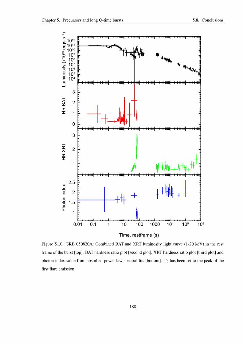
Chapter 5. Precursors and long Q-time bursts 5.8. Conclusions
104
105
106
107
108
109
1010
1011
1012
Lu
min
osity (
x1
04
0 e
rgs s
−1)
0
1
2
3
HR
BA
T
1
2
3
HR
XR
T
0.01 0.1 1 10 100 1000 104 105 106
1
1.5
2
2.5
Ph
oto
n in
de
x
Time, restframe (s)
Figure 5.10: GRB 050820A: Combined BAT and XRT luminosity light curve (1-20 keV) in the rest
frame of the burst [top]. BAT hardness ratio plot [second plot], XRT hardness ratio plot [third plot] and
photon index value from absorbed power law spectral fits [bottom]. T0 has been set to the peak of the
first flare emission.
188

Chapter 5. Precursors and long Q-time bursts 5.8. Conclusions
104
105
106
107
108
109
1010
1011
1012
Lu
min
osity (
x1
04
0 e
rgs s
−1)
0
1
2
3
HR
BA
T
0.5
1
HR
XR
T
0.01 0.1 1 10 100 1000 104 105 106
1.6
1.8
2
2.2
Ph
oto
n in
de
x
Time, restframe (s)
Figure 5.11: GRB 060115: Combined BAT and XRT luminosity light curve (1-20 keV) in the rest frame
of the burst [top]. BAT hardness ratio plot [second plot], XRT hardness ratio plot [third plot] and photon
index value from absorbed power law spectral fits [bottom]. Mode switching in the XRT occasionally
causes WT mode and PC mode data to be accumulated over concurrent time intervals. Photon index
data points [bottom panel] with overlapping temporal intervals are the result of this effect. T0 has been
set to the peak of the first flare emission.
189

Chapter 5. Precursors and long Q-time bursts 5.8. Conclusions
104105106107108109
101010111012
Lu
min
osity (
x1
04
0 e
rgs s
−1)
0
1
2
HR
BA
T
1
2
3
HR
XR
T
0.01 0.1 1 10 100 1000 104 105 106
1
1.5
2
2.5
Ph
oto
n in
de
x
Time, restframe (s)
Figure 5.12: GRB 060124: Combined BAT and XRT luminosity light curve (1-20 keV) in the rest
frame of the burst [top]. BAT hardness ratio plot [second plot], XRT hardness ratio plot [third plot] and
photon index value from absorbed power law spectral fits [bottom]. T0 has been set to the peak of the
first flare emission.
190

Chapter 5. Precursors and long Q-time bursts 5.8. Conclusions
104
105
106
107
108
109
1010
1011
1012
Lu
min
osity (
x1
04
0 e
rgs s
−1)
0
2
4
6
HR
BA
T
1
2
HR
XR
T
0.01 0.1 1 10 100 1000 104 105 106
1
2
3
Ph
oto
n in
de
x
Time, restframe (s)
Figure 5.13: GRB 060210: Combined BAT and XRT luminosity light curve (1-20 keV) in the rest
frame of the burst [top]. BAT hardness ratio plot [second plot], XRT hardness ratio plot [third plot] and
photon index value from absorbed power law spectral fits [bottom]. T0 has been set to the peak of the
first flare emission.
191
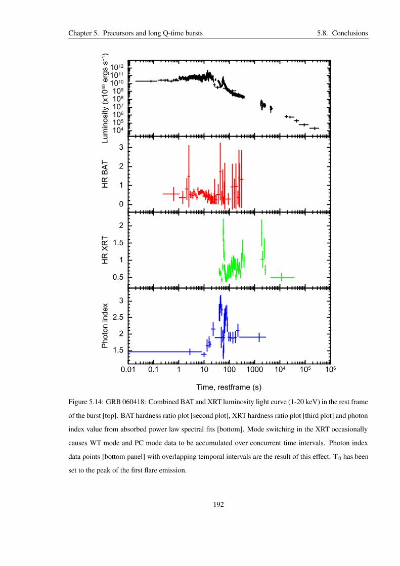
Chapter 5. Precursors and long Q-time bursts 5.8. Conclusions
104
105
106
107
108
109
1010
1011
1012
Lu
min
osity (
x1
04
0 e
rgs s
−1)
0
1
2
3
HR
BA
T
0.5
1
1.5
2
HR
XR
T
0.01 0.1 1 10 100 1000 104 105 106
1.5
2
2.5
3
Ph
oto
n in
de
x
Time, restframe (s)
Figure 5.14: GRB 060418: Combined BAT and XRT luminosity light curve (1-20 keV) in the rest frame
of the burst [top]. BAT hardness ratio plot [second plot], XRT hardness ratio plot [third plot] and photon
index value from absorbed power law spectral fits [bottom]. Mode switching in the XRT occasionally
causes WT mode and PC mode data to be accumulated over concurrent time intervals. Photon index
data points [bottom panel] with overlapping temporal intervals are the result of this effect. T0 has been
set to the peak of the first flare emission.
192
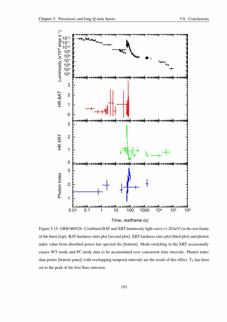
Chapter 5. Precursors and long Q-time bursts 5.8. Conclusions
104
105
106
107
108
109
1010
1011
1012
Lu
min
osity (
x1
04
0 e
rgs s
−1)
0
1
2
3
HR
BA
T
0
1
2
3
HR
XR
T
0.01 0.1 1 10 100 1000 104 105 106
1
2
3
Ph
oto
n in
de
x
Time, restframe (s)
Figure 5.15: GRB 060526: Combined BAT and XRT luminosity light curve (1-20 keV) in the rest frame
of the burst [top]. BAT hardness ratio plot [second plot], XRT hardness ratio plot [third plot] and photon
index value from absorbed power law spectral fits [bottom]. Mode switching in the XRT occasionally
causes WT mode and PC mode data to be accumulated over concurrent time intervals. Photon index
data points [bottom panel] with overlapping temporal intervals are the result of this effect. T0 has been
set to the peak of the first flare emission.
193

Chapter 5. Precursors and long Q-time bursts 5.8. Conclusions
104
105
106
107
108
109
1010
1011
1012
Lu
min
osity (
x1
04
0 e
rgs s
−1)
0
1
2
3
4
HR
BA
T
0.5
1
1.5
HR
XR
T
0.01 0.1 1 10 100 1000 104 105 106
1.5
2
2.5
Ph
oto
n in
de
x
Time, restframe (s)
Figure 5.16: GRB 060607A: Combined BAT and XRT luminosity light curve (1-20 keV) in the rest
frame of the burst [top]. BAT hardness ratio plot [second plot], XRT hardness ratio plot [third plot]
and photon index value from absorbed power law spectral fits [bottom]. Mode switching in the XRT
occasionally causes WT mode and PC mode data to be accumulated over concurrent time intervals.
Photon index data points [bottom panel] with overlapping temporal intervals are the result of this effect.
T0 has been set to the peak of the first flare emission.
194
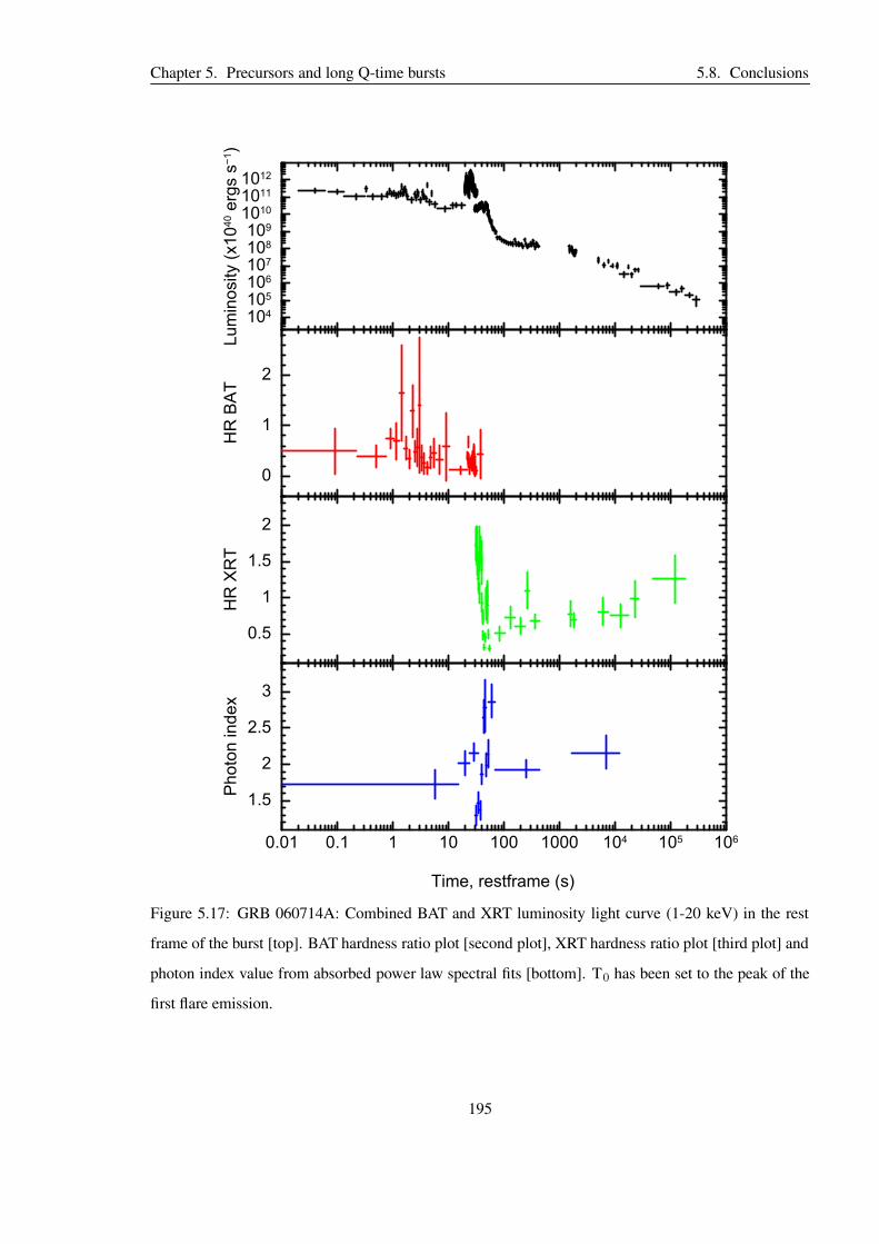
Chapter 5. Precursors and long Q-time bursts 5.8. Conclusions
104
105
106
107
108
109
1010
1011
1012
Lu
min
osity (
x1
04
0 e
rgs s
−1)
0
1
2
HR
BA
T
0.5
1
1.5
2
HR
XR
T
0.01 0.1 1 10 100 1000 104 105 106
1.5
2
2.5
3
Ph
oto
n in
de
x
Time, restframe (s)
Figure 5.17: GRB 060714A: Combined BAT and XRT luminosity light curve (1-20 keV) in the rest
frame of the burst [top]. BAT hardness ratio plot [second plot], XRT hardness ratio plot [third plot] and
photon index value from absorbed power law spectral fits [bottom]. T0 has been set to the peak of the
first flare emission.
195

Chapter 5. Precursors and long Q-time bursts 5.8. Conclusions
104
105
106
107
108
109
1010
1011
1012
Lu
min
osity (
x1
04
0 e
rgs s
−1)
0
0.5
1
HR
BA
T
1
2
3
4
HR
XR
T
0.01 0.1 1 10 100 1000 104 105 106
1
2
3
4
Ph
oto
n in
de
x
Time, restframe (s)
Figure 5.18: GRB 060904B: Combined BAT and XRT luminosity light curve (1-20 keV) in the rest
frame of the burst [top]. BAT hardness ratio plot [second plot], XRT hardness ratio plot [third plot]
and photon index value from absorbed power law spectral fits [bottom]. Mode switching in the XRT
occasionally causes WT mode and PC mode data to be accumulated over concurrent time intervals.
Photon index data points [bottom panel] with overlapping temporal intervals are the result of this effect.
T0 has been set to the peak of the first flare emission.
196

Chapter 5. Precursors and long Q-time bursts 5.8. Conclusions
104
105
106
107
108
109
1010
1011
1012
Lu
min
osity (
x1
04
0 e
rgs s
−1)
0
1
2
3
HR
BA
T
1
2
3
4
HR
XR
T
0.01 0.1 1 10 100 1000 104 105 106
2
4
6
8
Ph
oto
n in
de
x
Time, restframe (s)
Figure 5.19: GRB 061121: Combined BAT and XRT luminosity light curve (1-20 keV) in the rest frame
of the burst [top]. BAT hardness ratio plot [second plot], XRT hardness ratio plot [third plot] and photon
index value from absorbed power law spectral fits [bottom]. Mode switching in the XRT occasionally
causes WT mode and PC mode data to be accumulated over concurrent time intervals. Photon index
data points [bottom panel] with overlapping temporal intervals are the result of this effect. T0 has been
set to the peak of the first flare emission.
197

Chapter 5. Precursors and long Q-time bursts 5.8. Conclusions
5.B Appendix: Emission pulse fits.
BN (×10−8 ergs cm−2 s−1) ST (s) PT (s) DT (s)
GRB 050319
7.14+4.13−4.13 0.01(−) 0+0.01
−0.03 0.03+0.03−0.01
2.87+0.49−0.59 1.15+0.37
−0.43 2.72+0.08−0.08 0.13+0.09
−0.08
2.61+0.90−0.56 2.99+0.25
−0.24 3.40+0.12−0.04 0.35+0.11
−0.27
1.76+0.41−0.49 5.62+1.06
−0.39 8.44+0.73−0.43 0.78+0.01
−0.01
10.80+3.10−9.10 25.41(−) 31.67+0.09
−0.47 1.75+0.40−0.33
GRB 050820A
2.14+0.41−0.42 −1.16+0.40
−0.67 0+0.14−0.24 0.76+0.68
−0.31
2.14+0.38−0.40 1.46+0.23
−0.47 2.43+0.21−0.13 1.54+0.46
−0.42
0.90+0.03−0.03 60.07+0.51
−0.16 64.34+0.24−0.12 3.86(−)
GRB 060115
1.56+0.20−0.19 −4.77+1.71
−0.58 0+0.33−0.48 2.44+0.90
−0.76
2.36+0.16−0.17 16.74+0.31
−0.47 20.02+0.20−0.12 2.07+0.17
−0.28
(3.31+0.80−0.78) × 10−2 79.73+5.32
−5.56 85.24+4.92−3.08 16.15+7.09
−4.60
GRB 060124
2.72+0.96−1.07 −0.39+0.23
−0.12 0.0+0.04−0.03 1.92 × 10⁻²(−)
2.85+0.77−0.80 0.09+0.05
−0.10 0.28+0.11−0.08 0.41+0.20
−0.18
37.60+14.70−14.50 0.72+0.11
−0.08 0.92+0.10−0.13 0.27+0.10
−0.09
39.00+9.80−9.70 1.79+0.27
−0.35 1.18+0.33−0.44 1.51+0.49
−0.51
(1.68+0.30−0.30) × 10−2 53.58+6.67
−7.88 91.62+1.13−1.29 2.00+2.12
−1.31
0.33+0.05−0.05 94.82+1.61
−2.00 111.73+1.28−1.32 6.29+2.52
−1.99
0.38+0.04−0.05 114.54+3.37
−3.13 145.71+0.50−0.40 1.43+0.82
−0.68
Continued on Next Page. . .
198

Chapter 5. Precursors and long Q-time bursts 5.8. Conclusions
Table 5.12 – Continued
BN (×10−8 ergs cm−2 s−1) ST (s) PT (s) DT (s)
0.65+0.08−0.07 146.53+1.00
−1.22 156.75+0.06−0.04 (2.64+0.05
−0.07) × 10−2
1.69+0.09−0.08 153.09+0.42
−0.38 160.89+0.12−0.08 0.49+0.11
−0.10
0.65+0.05−0.07 159.67+1.06
−0.76 164.95+0.86−0.44 6.66+2.47
−0.54
3.67+0.24−0.09 166.85+0.06
−0.04 167.92+0.05−0.07 1.66+0.03
−0.20
9.21+0.34−0.14 171.20+0.04
−0.03 171.27+0.02−0.05 1.96+0.06
−0.06
0.38+0.05−0.07 179.54+1.37
−2.83 182.47+1.44−0.56 11.23+3.53
−2.23
0.32+0.10−0.10 194.77+2.24
−1.06 198.44+1.00−0.87 2.54+1.71
−1.27
1.65+0.14−0.05 205.30+0.01
−0.29 210.54+0.47−0.53 4.90+0.93
−0.82
0.12+0.01−0.01 288.01+0.79
−0.61 298.54+0.86−1.84 12.26+136.44
−6.21
GRB 060210
0.32+0.14−0.13 −0.16(−) 0+0.22
−0.47 0.84+0.57−0.45
0.18+0.03−0.03 30.19+0.50
−0.41 32.71+0.40−0.19 0.94+0.32
−0.26
0.44+0.02−0.02 34.47+0.38
−0.33 43.12+0.43−0.39 14.90+0.69
−0.70
0.78+0.09−0.09 39.64+0.29
−0.39 40.59+0.13−0.16 1.55+0.32
−0.29
2.02+0.19−0.19 45.19+0.07
−0.05 45.80+0.03−0.05 0.20+0.05
−0.04
0.29+0.02−0.02 61.18(−) 63.17+0.50
−0.57 8.26+0.51−0.49
0.32+0.01−0.01 78.63+0.30
−0.35 86.51+0.26−0.28 8.44+0.41
−0.41
0.25+0.01−0.01 111.62+0.76
−0.54 122.46+0.42−0.48 12.54+0.49
−0.48
GRB 060418
5.39+0.15−0.15 −0.87+0.20
−0.21 4.16+0.13−0.14 5.30+0.33
−0.36
2.92+0.92−0.93 −0.29+0.11
−0.22 0+0.01−0.01 0.001(−)
3.64+0.31−0.32 8.46+0.11
−0.17 9.47+0.23−0.26 5.59+0.92
−0.83
21.60+0.09−0.09 13.11+0.03
−0.04 13.64+0.03−0.04 0.61+0.03
−0.04
Continued on Next Page. . .
199

Chapter 5. Precursors and long Q-time bursts 5.8. Conclusions
Table 5.12 – Continued
BN (×10−8 ergs cm−2 s−1) ST (s) PT (s) DT (s)
7.69+1.16−0.74 15.32+0.15
−0.20 17.11+0.21−0.75 2.93+0.69
−0.16
1.58+0.12−0.12 35.00(−) 35.55+0.41
−0.49 5.85+0.38−0.38
2.03+0.07−0.08 51.56+0.14
−0.16 54.05+0.21−0.18 8.11+0.20
−0.22
GRB 060526
9.28+2.34−1.54 −0.01+0.01
−0.01 0+0.02−0.01 0.39+0.11
−0.12
1.09+0.05−0.05 53.96+0.20
−0.20 58.06+0.15−0.25 5.98+0.66
−0.49
0.65+0.01−0.04 64.47+0.51
−0.41 76.98+0.16−0.42 7.48+0.37
−0.33
GRB 060607A
1.55+0.05−0.06 −1.49+0.08
−0.06 0+0.07−0.08 2.15+0.14
−0.14
1.04+0.08−0.83 3.02+0.18
−0.16 4.90+0.21−0.28 3.03+0.37
−0.41
0.16+0.01−0.01 6.15+4.70
−4.79 20.39+0.44−0.57 5.11+0.52
−0.75
0.39+0.20−0.19 11.04+0.91
−1.06 13.27(−) 0.09+0.30−0.08
0.29+0.02−0.02 22.77+0.11
−0.15 23.30+0.15−0.13 4.80+0.30
−0.30
(4.87+0.34−0.40) × 10−2 33.10+2.37
−1.71 44.45+1.47−1.15 29.88+1.95
−3.16
0.26+0.10−0.10 53.25+0.57
−0.45 64.68+0.58−0.33 7.11+0.37
−0.35
GRB 060714A
3.54+0.60−0.65 −0.68+0.11
−0.17 0+0.01−0.07 0.50+0.19
−0.15
2.10+0.43−0.44 0.56+0.22
−0.36 0.87+0.17−0.18 1.69+0.54
−0.48
2.32+0.97−0.97 1.17+0.23
−0.23 1.66+0.11−0.08 0.09+0.01
−0.01
1.49+0.35−0.36 2.19(−) 1.58+0.87
−1.06 3.97+1.12−1.02
0.77+0.04−0.05 7.64+2.93
−3.23 19.45+0.59−0.65 10.62+0.38
−0.35
9.64+0.63−0.62 19.55+0.16
−0.21 21.13+0.07−0.07 1.00+0.14
−0.14
8.01+1.46−1.46 21.79+0.07
−0.08 22.29+0.03−0.04 0.08+0.05
−0.04
Continued on Next Page. . .
200

Chapter 5. Precursors and long Q-time bursts 5.8. Conclusions
Table 5.12 – Continued
BN (×10−8 ergs cm−2 s−1) ST (s) PT (s) DT (s)
18.20+1.20−1.10 23.48+0.15
−0.10 25.26+0.07−0.07 0.65+0.08
−0.07
9.28+1.01−1.06 25.22+0.25
−0.37 27.84+0.14−0.07 0.29+0.05
−0.07
0.43+0.02−0.02 29.51+0.39
−0.47 39.69+0.36−0.31 6.03+0.37
−0.41
0.45+0.03−0.03 43.94+0.44
−0.44 48.51+0.18−0.23 2.13+0.22
−0.21
GRB 060904B
4.16+0.46−0.50 −1.44+0.53
−2.20 0+0.18−0.13 2.09+0.31
−0.28
1.66+0.11−0.07 77.54+0.30
−0.31 93.36+0.88−1.47 23.61+2.10
−2.05
0.39+0.06−0.05 122.39+0.31
−0.39 122.90+0.50−0.40 16.38+3.09
−3.28
GRB 061121
6.28+0.53−0.52 −1.41+0.21
−0.41 0+0.08−0.10 0.88+0.14
−0.12
7.57+0.22−0.20 25.02+0.04
−0.04 25.64+0.02−0.02 1.29+0.12
−0.07
5.42+0.14−0.12 27.39+0.09
−0.06 28.29+0.05−0.03 3.79+0.27
−0.30
10.90+0.20−0.20 29.48+0.07
−0.05 31.41+0.01−0.02 0.37+0.03
−0.03
(2.78+0.38−0.36) × 10−2 33.40(−) 29.52+0.03
−0.01 1.66+0.34−0.29
1.54+0.18−0.40 36.90+0.35
−0.65 39.78+0.40−0.34 3.11+1.42
−1.42
0.65+0.02−0.28 45.89+1.84
−13.00 50.50+0.83−1.11 5.81+0.48
−0.48
Continued on Next Page. . .
201

Chapter 5. Precursors and long Q-time bursts 5.8. Conclusions
Table 5.12 – Continued
BN (×10−8 ergs cm−2 s−1) ST (s) PT (s) DT (s)
Table 5.12: Summary of emission pulse properties as modelled
by the FRED/BURS component in QDP, where T0 is taken to be
the peak of first emission pulse (SNR = 3). All fits are from BAT
data unless otherwise stated. BN is the normalisation of the BURS
component (or ‘peak’ flux), ST is the start time, PT the peak time
and DT is the decay constant of the exponential decay (see equa-
tion 5.1 for a further definition of the FRED/BURS component).
All times are quoted in the rest frame of the burst.
202