The Sparse Awakens: Streaming Algorithms forMatching Size Estimation in Sparse GraphsGraham Cormode1, Hossein Jowhari2, Morteza Monemizadeh3,and S. Muthukrishnan4

1 University of Warwick, UK. g.cormode@warwick.ac.uk. ∗

2 University of Warwick, UK. H.Jowhari@warwick.ac.uk. †

3 Amazon, Palo Alto, CA, USA. mmorteza@amazon.com. ‡

4 Rutgers University, Piscataway, NJ, USA. muthu@cs.rutgers.edu.

AbstractEstimating the size of the maximum matching is a canonical problem in graph analysis, and onethat has attracted extensive study over a range of different computational models. We presentimproved streaming algorithms for approximating the size of maximum matching with sparse(bounded arboricity) graphs.

(Insert-Only Streams) We present a one-pass algorithm that takes O(α logn) space and ap-proximates the size of the maximum matching in graphs with arboricity α within a factorof O(α). This improves significantly upon the state-of-the-art O(αn2/3)-space streaming al-gorithms, and is the first poly-logarithmic space algorithm for this problem.(Dynamic Streams) Given a dynamic graph stream (i.e., inserts and deletes) of edges of anunderlying α-bounded arboricity graph, we present an one-pass algorithm that uses spaceO(α10/3n2/3) and returns an O(α)-estimator for the size of the maximum matching on thecondition that the number edge deletions in the stream is bounded by O(αn). For this classof inputs, our algorithm improves the state-of-the-art O(αn4/5)-space algorithms, where theO(.) notation hides logarithmic in n dependencies.

In contrast to prior work, our results take more advantage of the streaming access to theinput and characterize the matching size based on the ordering of the edges in the stream inaddition to the degree distributions and structural properties of the sparse graphs.

1998 ACM Subject Classification G.2.2 Graph Theory

Keywords and phrases streaming algorithms; matching size

Digital Object Identifier 10.4230/LIPIcs.ESA.2017.<1>

1 Introduction

In this paper, we address a core graph analysis question of finding the size of a maximummatching, using space asymptotically smaller than even the number of nodes. Graphsnaturally capture relationships between entities, whether entities of the same type (simplegraphs), of two types (bipartite graphs), or other combinations of types (encoded viamultigraphs and hypergraphs). In modern applications, it is not uncommon to encounter

∗ Supported in part by European Research Council grant ERC-2014-CoG 647557, The Alan TuringInstitute under the EPSRC grant EP/N510129/1, and a Royal Society Wolfson Research Merit Award.

† Supported by European Research Council grant ERC-2014-CoG 647557.‡ Work was done when the author was at Rutgers University, Piscataway, NJ, USA.

© Graham Cormode, Hossein Jowhari, Morteza Monemizadeh, S. Muthukrishnan;licensed under Creative Commons License CC-BY

25th Annual European Symposium on Algorithms (ESA 2017).Editors: Kirk Pruhs and Christian Sohler; Article No.<1>; pp.<1>:1–<1>:16

Leibniz International Proceedings in InformaticsSchloss Dagstuhl – Leibniz-Zentrum für Informatik, Dagstuhl Publishing, Germany

<1>:2 Streaming Algorithms for Matching Size Estimation in Sparse Graphs

graphs with many millions or billions of nodes (capturing the huge number of entities thatcan interact), and billions to trillions of edges (enumerating the vast number of possibleinteractions). This has led to significant interest in addressing traditional graph analysisproblems in novel computational models: external memory, parallel and streaming models.

Problems related to (maximum) matchings in graph have a long history in ComputerScience. They arise in many contexts, from choosing which advertisements to display toonline users [34], to characterizing properties of chemical compounds [42]. Stable matchingshave a suite of applications, from assigning students to universities, to arranging organdonations [41]. These have been addressed in a variety of different computational models,from the traditional RAM model, to more recent sublinear (property testing [38]) and externalmemory/parallel (e.g. MapReduce [25]) models. Matching has also been studied for a numberof classes of input graph, including general graphs, bipartite graphs, weighted graphs, andthose with some sparsity structure.

Our work focuses on the streaming case, where each edge is seen once only, and we arerestricted to space sublinear in the size of the graph (ie., the number of vertices). Thiscaptures the scenario when the number of edges is overwhelmingly large, such as whenanalyzing connections between a massive number of individuals in a communication or socialnetwork. Now the objective is to find (approximately) the size of the matching. That is,while we cannot hope to retrieve a full description of the matching in sublinear space, wecan hope to estimate how big the matching is. Even here, results for general graphs areeither weak or make assumptions about the input or the stream order. In this work, weseek to improve the guarantees by restricting to graphs that have some measure of sparsity –bounded arboricity, or bounded degree. This aligns with reality, where most massive graphshave asymptotically fewer than Θ(n2) edges. For example, in graphs that arise in the contextof social networks, most nodes have a degree that is less than a few hundred, as people canonly maintain this number of active connections (Dunbar’s number), although a few nodes(“celebrities”) have very high (in-)degree in the multi-millions.

Estimating the matching size for graphs in the streaming model has been the subjectof some study in the algorithms and data analysis community in recent years. Kapralov,Khanna, and Sudan [21] developed a streaming algorithm which computes an estimateof matching size for general graphs within a factor of O(polylog(n)) in the random-orderstreaming model using O(polylog(n)) space. In the random-order model, the input streamis assumed to be chosen uniformly at random from the set of all possible permutations ofthe edges. Esfandiari et al. [15] were the first to study streaming algorithms for estimatingthe size of matching in bounded arboricity graphs in the adversarial-order streaming model,where the algorithm is required to provide a good approximation for any ordering of edges.Graph arboricity is a measure to quantify the density of a given graph. A graph G(V,E)has arboricity α if the set E of its edges can be partitioned into at most α forests. Sincea forest on n nodes has at most n − 1 edges, a graph with arboricity α can have at mostα(n− 1) edges. Indeed, by a result of Nash-Williams [36, 37] this holds for any subgraph ofa α-bounded arboricity graph G. Formally, the Nash-Williams Theorem [36, 37] states that

α = maxU⊆V

|E(U)|(|U | − 1) ,

where |U | and |E(U)| are the number of nodes and edges in the subgraph induced by the nodesU , respectively. Several important families of graphs have constant arboricity. Examplesinclude planar graphs (that have arboricity α = 3), bounded genus graphs, bounded treewidth

Cormode, Jowhari, Monemizadeh, Muthukrishnan <1>:3

graphs, and more generally, graphs that exclude a fixed minor.1The important observation in [15] is that the size of matching in bounded arboricity

graphs can be approximately characterized by the number of high degree vertices (verticeswith degree above a fixed threshold) and the number of so-called shallow edges (edges withboth low degree endpoints). This characterization allows for estimation of the matching sizein sublinear space by taking samples from the vertices and edges of the graph. The work of[15] implements the characterization in O(αn2/3) space and gives a O(α) approximation of thematching size. Subsequent works [6, 30] consider alternative characterizations and improveupon the approximation factor however they do not result in major space improvements.

1.1 Our ContributionsWe present major improvements in the space usage of streaming algorithms for sparse graphs(α-bounded Arboricity Graphs). Our main result is a polylog space algorithm that beats thenε space bound of prior algorithms. More precisely, we show:

I Theorem 1. Let G(V,E) be a graph with arboricity bounded by α. Let S be an (adversarialorder) insertion-only stream of the edges of the underlying graph G. Let M∗ be the size ofthe maximum matching of G (or S interchangeably). Then, there is a randomized 1-passstreaming algorithm that outputs a (22.5α+ 6)(1 + ε)-approximation to M∗ with probabilityat least 1− δ and takes O( αε2 logn) space.

This result is notable, since it is the first demonstration that the polynomial space cost canbe beaten for matching size estimation, and shows a that polylogarithmic space is sufficientfor a constant factor approximation. Subsequent to our initial statement of results [10],McGregor and Vorotnikova have provided a new analysis of our algorithm to improve theconstants in the approximation factor to achieve a (α+ 2)(1 + ε) factor [32].

For the case of dynamic streams (i.e, streams of inserts and deletes of edges), we design adifferent algorithm using O(α10/3n2/3) space which improves the O(αn4/5)-space dynamic(insertion/deletion) streaming algorithms of [6, 7]. The following theorem states this result(proved in Section 3.3).

I Theorem 2. Let G(V,E) be a graph with the arboricity bounded by α. Let M∗ be the sizeof the maximum matching of G. Let S be a dynamic stream of edge insertions and deletionsof the underlying graph G of length at most O(αn). Let

β = µ(2µ)

(µ− 2α+ 1) + 1 where µ > 2α.

Then, there exists a streaming algorithm that takes O(β4/3(nα)2/3

ε4/3 ) space in expectation andoutputs a (1 + ε)β approximation of M∗ with probability at least 0.86.

Quite recently Assadi et al. [3] gave an Ω(n1/2

α2.5 ) space lower bound for getting a c-approximation of the matching size in dynamic graph streams with arboricity bounded by α.We obtain our n2/3 bound by first defining an algorithm for insert-only streams with as n1/2

behavior, which suggests that this could also be feasible in the dynamic setting.Our algorithms for bounded arboricity graphs are based on two novel streaming-friendly

characterizations of the maximum maching size. The first characterization is a modification

1 For any H-minor-free graph, the arboricity is O(h√h) where h is the number of vertices of H. [24]

ESA 2017

<1>:4 Streaming Algorithms for Matching Size Estimation in Sparse Graphs

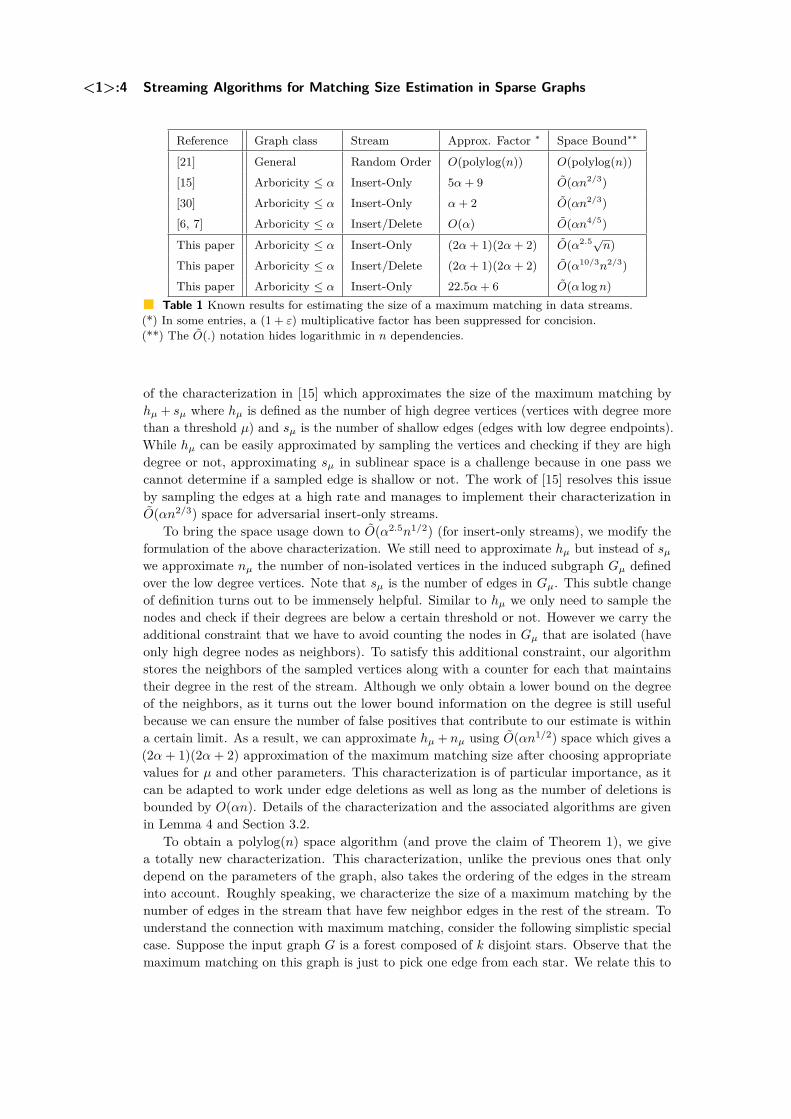
Reference Graph class Stream Approx. Factor ∗ Space Bound∗∗

[21] General Random Order O(polylog(n)) O(polylog(n))

[15] Arboricity ≤ α Insert-Only 5α+ 9 O(αn2/3)

[30] Arboricity ≤ α Insert-Only α+ 2 O(αn2/3)

[6, 7] Arboricity ≤ α Insert/Delete O(α) O(αn4/5)

This paper Arboricity ≤ α Insert-Only (2α+ 1)(2α+ 2) O(α2.5√n)

This paper Arboricity ≤ α Insert/Delete (2α+ 1)(2α+ 2) O(α10/3n2/3)

This paper Arboricity ≤ α Insert-Only 22.5α+ 6 O(α logn)Table 1 Known results for estimating the size of a maximum matching in data streams.

(*) In some entries, a (1 + ε) multiplicative factor has been suppressed for concision.(**) The O(.) notation hides logarithmic in n dependencies.

of the characterization in [15] which approximates the size of the maximum matching byhµ + sµ where hµ is defined as the number of high degree vertices (vertices with degree morethan a threshold µ) and sµ is the number of shallow edges (edges with low degree endpoints).While hµ can be easily approximated by sampling the vertices and checking if they are highdegree or not, approximating sµ in sublinear space is a challenge because in one pass wecannot determine if a sampled edge is shallow or not. The work of [15] resolves this issueby sampling the edges at a high rate and manages to implement their characterization inO(αn2/3) space for adversarial insert-only streams.

To bring the space usage down to O(α2.5n1/2) (for insert-only streams), we modify theformulation of the above characterization. We still need to approximate hµ but instead of sµwe approximate nµ the number of non-isolated vertices in the induced subgraph Gµ definedover the low degree vertices. Note that sµ is the number of edges in Gµ. This subtle changeof definition turns out to be immensely helpful. Similar to hµ we only need to sample thenodes and check if their degrees are below a certain threshold or not. However we carry theadditional constraint that we have to avoid counting the nodes in Gµ that are isolated (haveonly high degree nodes as neighbors). To satisfy this additional constraint, our algorithmstores the neighbors of the sampled vertices along with a counter for each that maintainstheir degree in the rest of the stream. Although we only obtain a lower bound on the degreeof the neighbors, as it turns out the lower bound information on the degree is still usefulbecause we can ensure the number of false positives that contribute to our estimate is withina certain limit. As a result, we can approximate hµ + nµ using O(αn1/2) space which gives a(2α+ 1)(2α+ 2) approximation of the maximum matching size after choosing appropriatevalues for µ and other parameters. This characterization is of particular importance, as itcan be adapted to work under edge deletions as well as long as the number of deletions isbounded by O(αn). Details of the characterization and the associated algorithms are givenin Lemma 4 and Section 3.2.

To obtain a polylog(n) space algorithm (and prove the claim of Theorem 1), we givea totally new characterization. This characterization, unlike the previous ones that onlydepend on the parameters of the graph, also takes the ordering of the edges in the streaminto account. Roughly speaking, we characterize the size of a maximum matching by thenumber of edges in the stream that have few neighbor edges in the rest of the stream. Tounderstand the connection with maximum matching, consider the following simplistic specialcase. Suppose the input graph G is a forest composed of k disjoint stars. Observe that themaximum matching on this graph is just to pick one edge from each star. We relate this to

Cormode, Jowhari, Monemizadeh, Muthukrishnan <1>:5

a combinatorial characterization that arises from the sequence of edges in the stream: nomatter how we order the edges of G in the stream, from each star there is exactly one edgethat has no neighboring edges in the remainder of the stream (in other words, the last edge ofthe star in the stream). Our characterization generalizes this idea to graphs with arboricitybounded by α by counting the γ-good edges, i.e. edges that have at most γ = 6α neighborsin the remainder of the stream. We prove this characterization gives an O(α) approximationof the maximum matching size. More important, a nice feature of this characterization isthat it can be implemented in polylog(n) space if one allows a 1 + ε approximation. Theimplementation adapts an idea from the well-known L0 sampling algorithm. It runs O(logn)parallel threads each sampling the stream at a different rate. At the end, a thread “wins”that has sampled roughly Θ(logn) elements from the γ-good edges (samples the edges witha rate of logn

k where k is the number of γ-good edges). The threads that under-sample willend up with few edges or nothing while the ones that have oversampled will keep too manyγ-good edges and will be terminated as soon as they hit a space threshold as a result. Table 1summarizes the known and new results for estimating the size of a maximum matching.

1.2 Related WorkWe discuss the most relevant work to matching size estimation earlier in the introduction.Here, we give an overview of related work by providing the context of matching and streamingalgorithms in general, before focusing in on the most related works at the intersection. Theproblem of computing the maximum matching of G has been extensively studied in theclassical offline model, where we assume we have enough space to store all vertices and edgesof a graph G = (V,E). The classical result in this model is the algorithm due to Micali andVazirani [35] with running time O(m

√n), where n = |V | and m = |E|. Recent work has given

improved results for sparse bipartite graphs [27]. A matching of size within (1− ε) factor ofa maximum cardinality matching can be found in O(m/ε) time [19, 35]. Recently, Duan andPettie [12] developed a (1− ε)-approximate maximum weighted matching algorithm in timeO(m/ε).

The model of streaming data analysis has received a similar level of scrutiny. A survey byMcGregor [31] gives an overview of results in the graph streaming model. Many fundamentalquestions have been tackled: counting the number of occurrences of specific small subgraphssuch as triangles [33]; estimating properties of neighborhoods [8]; and using ‘sketch’ techniquesto track local and global properties of graphs like connectivity [2].

The question of finding an approximation to the maximum cardinality matching has beenextensively studied in the streaming model. An O(n)-space greedy algorithm trivially obtainsa maximal matching, which is a 2-approximation for the maximum cardinality matching [16].A natural question is whether one can beat the approximation factor of the greedy algorithmwith O(n polylog(n)) space. Recently, it was shown that obtaining an approximation factorbetter than e

e−1 ' 1.58 in one pass requires n1+Ω(1/ log logn) space [17, 20], even in bipartitegraphs and in the vertex-arrival model, where the vertices arrive in the stream together withtheir incident edges. This setting has also been studied in the context of online algorithms,where each arriving vertex has to be either matched or discarded irrevocably upon arrival.Seminal work due to Karp, Vazirani and Vazirani [22] gives an online algorithm with e

e−1approximation factor in this model.

Closing the gap between the upper bound of 2 and the lower bound of ee−1 remains

one of the most appealing open problems in the graph streaming area (see [39]). Thefactor of 2 can be improved on if one either considers the random-order model or allows fortwo passes [23]. By allowing even more passes, the approximation factor can be improved

ESA 2017

<1>:6 Streaming Algorithms for Matching Size Estimation in Sparse Graphs

to multiplicative (1 − ε)-approximation via finding and applying augmenting paths withsuccessive passes [28, 29, 13, 1].

Another line of research [16, 28, 43, 14, 11] has explored the question of approximatingthe maximum-weight matching in one pass and O(n polylog(n)) space. The latest resultis that a (2 + ε) approximation factor is possible using an O(n logn) space deterministicalgorithm, essentially meeting the unweighted matching case [40]. These results are for theinsert-only case. Where deletions are allowed (the dynamic, or turnstile case), the problemis harder: Ω(n2−3ε) space is needed to provide an O(nε) approximation [5]; and Ω(n/α2) toprovide an O(α) approximation [4]. However, our focus is on finding the size of the maximummatching without materializing it, and so our aim is for sublinear space algorithms.

2 Preliminaries and Notations

Let G(V,E) be an undirected unweighted graph with n = |V | vertices and m = |E| edges.For a vertex v ∈ V , let degG(v) denote the degree of vertex v in G. A matching M of G isa set of pairwise non-adjacent edges, i.e., no two edges share a common vertex. Edges inM are called matched edges; the other edges are called unmatched. A maximum matchingof graph G(V,E) is a matching of maximum size. Throughout the paper, when we fix amaximum matching of G(V,E), we denote it by M∗. A matching M of G is maximal if it isnot a proper subset of any other matching in graph G. Abusing the notation, we sometimesuse M∗ and M for the size of the maximum and maximal matching, respectively. It iswell-known (see for example [26]) that the size of a maximal matching is at least half ofthe size of a maximum matching, i.e., M ≥ M∗/2. Thus, we say a maximal matching isa 2-approximation of a maximum matching of G. It is known [26] that the simple greedyalgorithm, where we include each new edge if neither of its endpoints are already matched,returns a maximal matching.

3 Algorithms for Bounded Arboricity Graphs

Throughout this section, hµ denotes the number of vertices in graph G = (V,E) that havedegree above µ. Let Gµ = (L,F ) be the induced subgraph of G where L = v| degG(v) ≤ µand (u, v) ∈ F ⊆ E when u and v are both in L. Note that Gµ might have isolated vertices.In the following we let Mµ denote the size of maximum matching in Gµ.

3.1 Characterization lemmasI Lemma 3 ([15]). For a α-bounded arboricity graph G(V,E) and µ > 2α, we have hµ ≤

2µµ−2α+1M

∗.

I Lemma 4. For a α-bounded arboricity graph G(V,E) and µ > 2α, we have

M∗ ≤ hµ +Mµ ≤(

2µµ− 2α+ 1 + 1

)M∗ .

Proof. The lower bound is easy to see: every edge of a maximum matching either has anendpoint with degree more than µ or both of its endpoints are vertices with degree at mostµ. The number of matched edges of the first type are bounded by hµ whereas the number ofmatched edges of the second type are bounded by Mµ.

To prove the upper bound, we use the fact Mµ ≤M∗ and Lemma 3. J

Cormode, Jowhari, Monemizadeh, Muthukrishnan <1>:7

I Definition 5. Let S = (e1, . . . , em) be a sequence of edges. We say the edge ei = (u, v) isγ-good with respect to S if maxdi(u), di(v) ≤ γ where di(x) is defined as |ej |j > i, ej =(x,w)|, i.e. the number of edges incident on x that appear after the i-th edge in the stream.We write Eγ(S) as the set of γ-good edges in S, and usually drop (S) in context.

To illustrate the power of this definition, we first consider the case of trees. Trees are agood test case for understanding matchings, since they can have widely varying matchingsizes: from 1 (a star graph on n nodes) to O(n) (a path of length n or a binary tree on nnodes). In fact the following lemma suggests that counting the number of 1-good edges givesa 2 factor approximation to the matching size on trees. (Due to the space limitations wehave deferred the proof of this lemma to the full version of this paper.)

I Lemma 6. For trees we have M∗ ≤ |E1| ≤ 2M∗.

Our main result on γ-goodness is for general graphs with α-bounded arboricity.

I Lemma 7. Let µ > 2α be a (large enough) integer, and let Eγ be the set of γ-good edgesin an edge stream for a graph with arboricity at most α. We have:

(12 −

α

µ+ 1

)M∗ ≤ |Eγ | ≤

(54γ + 2

)M∗,

where γ = maxµ− 1, 4α(µ+1)µ+1−2α. In particular for µ = 6α− 1, we have

M∗ ≤ 3|E6α| ≤ (22.5α+ 6)M∗

Proof. First we prove the lower bound on |Eγ |. In particular we show a relation involving thenumber of edges where both endpoints have low degree. Define hµ = |v|v ∈ V,degG(v) > µ|,and sµ = |e = (u, v)|e ∈ E,degG(u) ≤ µ, degG(v) ≤ µ|, i.e. the number of edges in thegraph Gµ. Then:(

12 −

α

µ+ 1

)hµ + sµ ≤ |Eγ |.

The claim in the lemma follows from the relatively loose bound that M∗ ≤ hµ + sµ. LetH be the set of vertices in the graph with degree above µ and let L = V \H. Recall thathµ = |H|. Let H0 be the vertices in H that have no neighbor in L, and let H1 = H \H0.First we notice that |H1| ≥ (1 − 2α

µ )|H|. To see this, let E′ be the edges with at leastone endpoint in H0. By definition, every node in H0 has degree at least µ+ 1, so we have|E′| ≥ µ+1

2 |H0|. At the same time, the total number of edges in the subgraph induced bythe nodes H is at most α(|H| − 1), using the arboricity assumption. Therefore,

α(|H| − 1) ≥ |E′| ≥ 12 (µ+ 1)|H0|

It follows that |H0| ≤ 2αµ+1 (|H| − 1) which further implies that

|H1| ≥ (1− 2αµ+ 1)|H| = (1− 2α

µ+ 1)hµ. (1)

Now let degH(v) be the degree of v in the subgraph induced by H. We have∑v∈H1

degH(v) ≤ 2α|H|, again using the arboricity bound and the fact that summingover degrees counts each edge at most twice. Therefore, taking the average over nodes in H1,

degH(v) ≤ 2α1− 2α

µ+1

ESA 2017

<1>:8 Streaming Algorithms for Matching Size Estimation in Sparse Graphs

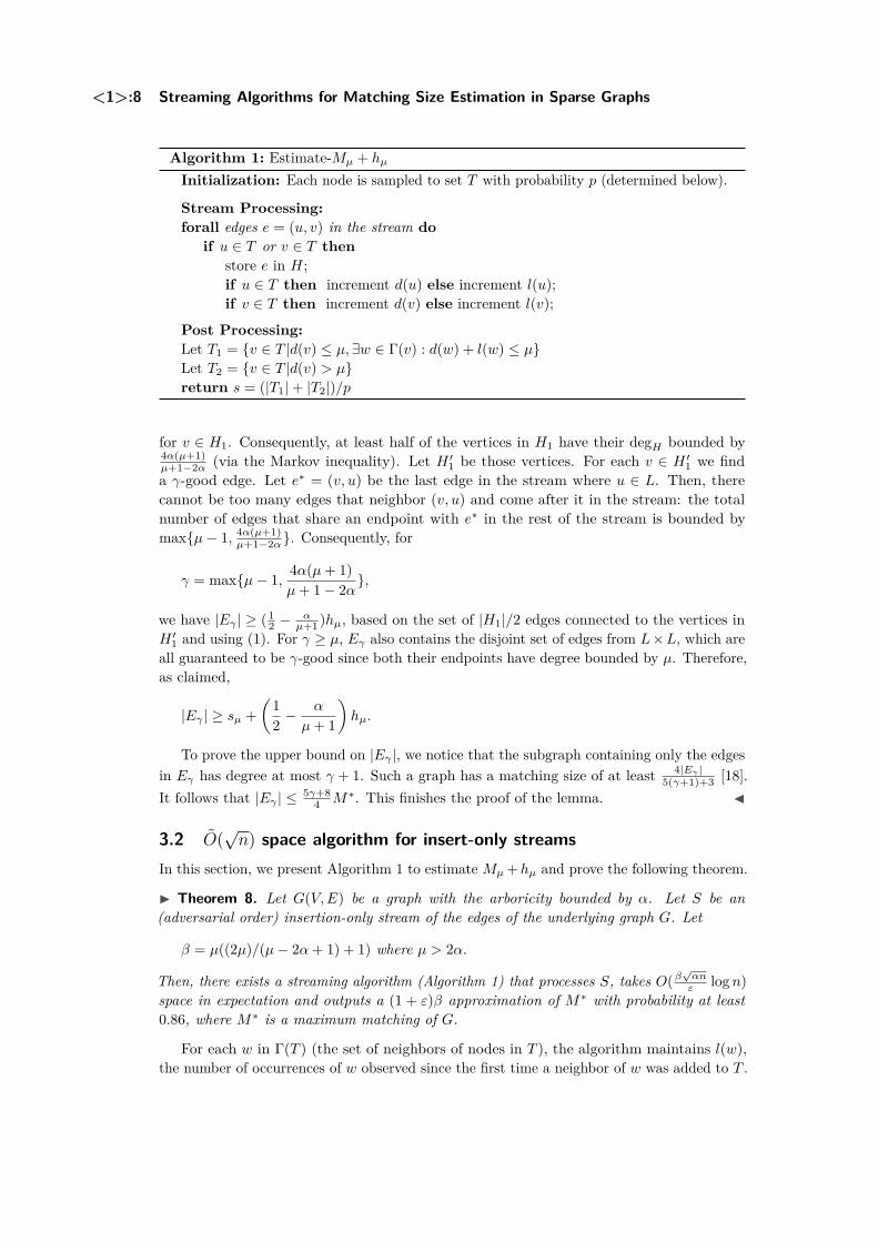
Algorithm 1: Estimate-Mµ + hµ

Initialization: Each node is sampled to set T with probability p (determined below).

Stream Processing:forall edges e = (u, v) in the stream do

if u ∈ T or v ∈ T thenstore e in H;if u ∈ T then increment d(u) else increment l(u);if v ∈ T then increment d(v) else increment l(v);

Post Processing:Let T1 = v ∈ T |d(v) ≤ µ, ∃w ∈ Γ(v) : d(w) + l(w) ≤ µLet T2 = v ∈ T |d(v) > µreturn s = (|T1|+ |T2|)/p

for v ∈ H1. Consequently, at least half of the vertices in H1 have their degH bounded by4α(µ+1)µ+1−2α (via the Markov inequality). Let H ′1 be those vertices. For each v ∈ H ′1 we finda γ-good edge. Let e∗ = (v, u) be the last edge in the stream where u ∈ L. Then, therecannot be too many edges that neighbor (v, u) and come after it in the stream: the totalnumber of edges that share an endpoint with e∗ in the rest of the stream is bounded bymaxµ− 1, 4α(µ+1)

µ+1−2α. Consequently, for

γ = maxµ− 1, 4α(µ+ 1)µ+ 1− 2α,

we have |Eγ | ≥ ( 12 −

αµ+1 )hµ, based on the set of |H1|/2 edges connected to the vertices in

H ′1 and using (1). For γ ≥ µ, Eγ also contains the disjoint set of edges from L×L, which areall guaranteed to be γ-good since both their endpoints have degree bounded by µ. Therefore,as claimed,

|Eγ | ≥ sµ +(

12 −

α

µ+ 1

)hµ.

To prove the upper bound on |Eγ |, we notice that the subgraph containing only the edgesin Eγ has degree at most γ + 1. Such a graph has a matching size of at least 4|Eγ |

5(γ+1)+3 [18].It follows that |Eγ | ≤ 5γ+8

4 M∗. This finishes the proof of the lemma. J

3.2 O(√

n) space algorithm for insert-only streamsIn this section, we present Algorithm 1 to estimate Mµ +hµ and prove the following theorem.

I Theorem 8. Let G(V,E) be a graph with the arboricity bounded by α. Let S be an(adversarial order) insertion-only stream of the edges of the underlying graph G. Let

β = µ((2µ)/(µ− 2α+ 1) + 1) where µ > 2α.

Then, there exists a streaming algorithm (Algorithm 1) that processes S, takes O(β√αnε logn)

space in expectation and outputs a (1 + ε)β approximation of M∗ with probability at least0.86, where M∗ is a maximum matching of G.

For each w in Γ(T ) (the set of neighbors of nodes in T ), the algorithm maintains l(w),the number of occurrences of w observed since the first time a neighbor of w was added to T .

Cormode, Jowhari, Monemizadeh, Muthukrishnan <1>:9

Algorithm 2: Estimate-M∗

Initialization: Let ε ∈ (0, 1) and t = dβ√

8ncε e where β is as defined in Lemma 9.

Stream Processing: Do the following tasks in parallel:(1) Greedily keep a maximal matching of size at most r ≤ t (and terminate this task if this

size bound is exceeded).(2) Run the Estimate-(Mµ + hµ) procedure (Algorithm 1) with p ≥ 8

λ2t where λ = εβ .

Post processing: If r < t then output 2r as the estimate for M∗, otherwise outputthe result of the Estimate-(Mµ + hµ) procedure.

Note that in this algorithm, l(w) is a lower bound on the degree of w. For the output, T1 isthe subset of nodes in T whose degree is bounded by µ and additionally for each node in T1,there is a neighbor w whose observed degree (d(w) or l(w)) is at most µ. Meanwhile, T2 isthe set of “high degree” nodes in T .

I Lemma 9. Let ε ∈ (0, 1) and β = µ( 2µµ−2α+1 + 1). With probability at least 1− e

−ε2M∗p4β2 ,

Algorithm 1 outputs s where

(1− ε)M∗ ≤ s ≤ (1 + ε)βM∗.

Proof. First we prove the following bounds on E(s).

Mµ + hµ ≤ E(s) ≤ µ(Mµ + hµ).

Let L be the set of vertices in G that have degree at most µ and let GL be the induced graphon L. Let H = V \ L. Note that GL might have isolated vertices. Let N be the non-isolatedvertices in GL. It is clear that if the algorithm samples v ∈ N , v will be in T1. Likewise, if itsamples a vertex w ∈ H, w will be in T2. Given the fact that |H| = hµ and |N | ≥Mµ, thisproves the lower bound on E(s).

The expectation may be above Mµ, as the algorithm may pick an isolated vertex in GL(a vertex that is only connected to the high-degree vertices) and include it in T1 because oneof its high-degree neighbours w was identified as low degree, i.e., w ∈ Γ(T ) and l(w) ≤ µ butw ∈ H. Let u ∈ H and let U = a1, . . . , aµ be the last µ neighbours of u according to theordering of the edges in the stream. The algorithm can only identify u as low degree when itpicks a sample from U and no samples from Γ(u) \U . This restricts the number of unwantedisolated vertices to at most µhµ. Together with the fact that |N | ≤ µMµ, it establishes theupper bound on E(s). Now using a Chernoff bound,

Pr[|s− E(s)| ≥ λE(s)

]= Pr

[|s.p− E(s.p)| ≥ λE(s.p)

]≤ exp(−λ2(Mµ + hµ)p/4) ≤ exp(−λ2M∗p/4).

Therefore with probability at least 1− e−λ2M∗p

4 ,

(Mµ + hµ)− λµ(hµ +Mµ) ≤ s ≤ µ(1 + λ)(Mµ + hµ) (2)

Setting λ = εβ and combining with Lemma 4, we derive the statement of the lemma. J

Proof of Theorem 8: Suppose M∗ < t. Clearly the size of the maximal matching robtained by the first task will be less than t. In this case, M∗ ≤ 2r ≤ 2M∗. Now suppose

ESA 2017

<1>:10 Streaming Algorithms for Matching Size Estimation in Sparse Graphs

M∗ ≥ t. By Lemma 4, we will have Mµ + hµ ≥ t and hence by Lemma 9, with probability atleast 1− e−2 ≥ 0.86, the output of the algorithm will be within the promised bounds. Theexpected space of the algorithm is O((t+ pnα) logn). Setting t = β

√8nα/ε to balance the

space costs, the space complexity of the algorithm will be O(β√αnε logn) as claimed. 2

3.3 O(n2/3) space algorithm for insertion/deletion streamsAlgorithms 1 and 2 form the basis of our solution in the more general case where the streamcontains deletions of edges as well. In the case of Algorithm 1, the algorithm has to maintainthe induced subgraph on T and the edges of the cut (T,Γ(T )). However if we allow anarbitrary number of insertions and deletions, the size of the cut (T,Γ(T )) can grow as largeas O(n) even when |T | = 1. This is because each node at some intermediate point couldbecome high degree and then lose its neighbours because of the subsequent deletion of edges.Therefore here in order to limit the space usage of the algorithm, we make the assumptionsthat number of deletions is bounded by O(αn). Since the processed graph has arboricity atmost α this forces the number of insertions to be O(αn) as well. Under this assumption, ifwe pick a random vertex, still, in expectation the number of neighbours is bounded by O(α).

Another complication arises from the fact that, with edge deletions, a vertex added toΓ(T ) might become isolated at some point. In this case, we discard it from Γ(T ). Additionallyfor each vertex in T ∪Γ(T ), the counters d(v) (or l(v) depending on if it belongs to T or Γ(T ))can be maintained as before. The space complexity of the algorithm remains O(pnα logn) inexpectation as long as the arboricity factor remains within O(α) in the intermediate graphs.In the case of Algorithm 2, we need to keep a maximal matching of size O(t). This can bedone in O(t2) space using a randomized algorithm [7]. Setting t at ( 8βnα

ε2 )1/3 to rebalancethe space costs, we obtain the result of Theorem 2.

3.4 The polylog space algorithm for insert-only streamsIn this section we present our polylog space algorithm by presenting an algorithm forestimating |Eγ | within a (1 + ε) factor. Our algorithm is similar in spirit to the well-knownL0 sampling strategy [9]. We first describe it in terms of running O(logn) parallel threadseach sampling the stream at a different rate. At the end, a thread “wins” that has sampledroughly Θ(logn) elements from |Eγ | (samples the edges with a rate of logn

|Eγ | ). The threads thatunder-sample will end up with few edges or nothing while the ones that have oversampledwill keep too many elements of Eγ and will be aborted as result. Finally, we mention howa suitable implementation can reduce the space dependency to O(α logn) (treating ε asconstant).

First we give a simple subroutine (Algorithm 3) that is the building block of the algorithm.Given γ and an edge e in the stream, it simply counts up the number of subsequent edges thatare incident on either endpoint of e, and consequently determines whether e is in Eγ . Ourmain algorithm (Algorithm 4) samples edges, and applies this subroutine to them. Multiplesampling rates pi are used in parallel; however, if at any point the number of sampled edgesin a level exceeds a threshold τ , the level is “terminated”, and no further samples are takenat this level. This ensures that the space used remains bounded.

I Lemma 10. With high probability, Algorithm 4 outputs a 1±O(ε) approximation of |Eγ |where γ is defined according to Lemma 7.

Proof. Consider the sets of active γ-good tests at each level at the conclusion of the algorithm,Xi. First we observe that if |X0| ≤ τ then X0 = Eγ and the algorithm makes no error.

Cormode, Jowhari, Monemizadeh, Muthukrishnan <1>:11

Algorithm 3: The γ-good testInitialization: given the edge e = (u, v) in the stream, let r(u) = 0 and r(v) = 0.forall subsequent edges e′ = (t, w) do

if u ∈ t, w then increment r(u);if v ∈ t, w then increment r(v);if maxr(u), r(v) > γ then terminate and report NOT γ-good;

Algorithm 4: An algorithm for approximating |Eγ |Initialization: ∀i.Xi = ∅ . Xi represents the current set of sampled γ-good edges.

Stream Processing:forall levels i ∈ 0, 1, . . . , [blog1+ε n

2c in parallel doforall edges e do

Feed e to the active γ-good tests and update Xi

With probability pi = 1(1+ε)i add e to Xi and start a γ-good test for e.

Let |Xi| be the number of active γ-good tests within this level.if |Xi| > τ = 64γ2 logn

αε2 then terminate level i;

Post processing:if |X0| ≤ τ then

return |X0|else . |X0| > τ

let j be smallest integer s.t. |Xj | ≤ 8 logn(1+ε)ε2 and j-th level was not terminated;

if there is no such j then return fail else return |Xj |pj

;

In case |Xi| > τ , we claim that |Eγ | > α2γ2 τ . To prove this, let t be the time step where

|Xi| exceeds τ (i.e. when this level is terminated) and let Gt = (V,E(t)) be the graphwhere E(t) = e1, . . . , et. Clearly M∗(G) ≥M∗(Gt) because the size of the matching onlyincreases as new edges arrive. Abusing the notation, let Eγ(Gt) denote the set of γ-goodedges at time t. By Lemma 7 and definition of γ, we have

τ < |Eγ(Gt)| ≤(

54γ + 2

)M∗(Gt) ≤ 4γM∗(G) ≤ 2(µ+ 1)

µ− 2α+ 14γ|Eγ | ≤( γ

2α

)4γ|Eγ |

(3)

This proves the claim that |Eγ | > α2γ2 τ when |Xi| > τ . Let τ ′ = 8 logn

ε2 and let i∗ be theinteger such that

(1 + ε)i∗−1τ ′ ≤ |Eγ | ≤ (1 + ε)i

∗τ ′.

Assuming the i∗-th level does not terminate before the end, we have τ ′

(1+ε) ≤ E[|Xi∗ |] ≤τ ′. By a Chernoff bound, for each i we have (again assuming we do not terminate thecorresponding level)

Pr[∣∣|Xi| − E(|Xi|)

∣∣ ≥ εE(|Xi|)]≤ exp

(−ε

2pi|Eγ |4

).

So, Pr[∣∣|Xi∗ | − E(|Xi∗ |)

∣∣ ≥ εE(|Xi∗ |)]≤ exp (− ε2|Eγ |

2(1 + ε)i∗ ) ≤ exp (2 logn1 + ε

) ≤ O(n−1).

ESA 2017

<1>:12 Streaming Algorithms for Matching Size Estimation in Sparse Graphs

As a result, with high probability |Xi∗ | ≤ 8 logn(1+ε)ε2 . Moreover for all i < i∗ − 1,

the corresponding levels either terminate prematurely or in the end we will have |Xi| >8 logn(1+ε)

ε2 with high probability. Consequently j ∈ i∗, i∗ − 1. It remains to prove thatruns corresponding to i∗ and i∗ − 1 will survive until the end with high probability. Weprove this for i∗. The case of i∗ − 1 is similar.

Consider a fixed time t in the stream and let X(t)i∗ be the set of sampled γ-good edges at

time t corresponding to the i∗-th level. Note that X(t)i∗ contains the a subset of γ-good edges

with respect to the stream St = (e1, . . . , et). From the definition of i∗ and Inequality (3) wehave

E[|X(t)i∗ |] = |Eγ(Gt)|

(1 + ε)i∗ ≤2γ2|Eγ |α(1 + ε)i∗ ≤

2γ2τ ′

α.

By the Chernoff inequality for δ ≥ 1,

Pr[|X(t)

i∗ | ≥ (1 + δ)E(|X(t)i∗ |)

]≤ exp

(−δ3 E(|X(t)

i∗ |)).

From δ = τ

E(|X(t)i∗ |)− 1 = τ(1+ε)i

∗

|Eγ(Gt)| − 1, we get

Pr[|X(t)

i∗ | ≥ τ]≤ exp

(−τ3 + |Eγ(Gt)|

(1 + ε)i∗)≤ exp

(−τ3 + 2γ2τ ′

α

)For τ ≥ 8γ2τ ′

α , the term inside the exponent is smaller than −2 logn. It also satisfiesδ ≥ 1. After applying the union bound, for all t the size of X(t)

i∗ is bounded by τ = 64γ2 lognαε2

with high probability. This finishes the proof of the lemma. J

Next, putting everything together, we prove Theorem 1.

Proof of Theorem 1: The theorem follows from Lemmas 7 and 10 and taking γ =µ+ 1 = 6α. Observe that the space cost of Algorithm 4 can be bounded: we have log1+ε n

2

levels where each level runs at most τ concurrent γ-good tests otherwise it will be terminated.Each γ-good test keeps an edge and two counters and as result it occupies O(1) space.Consequently the space usage of the algorithm is bounded by O(τ log1+ε n). Using the factthat τ = O( αε2 logn) for γ = 6α, we obtain a space bound of O( αε2 log2 n).

A simple implementation optimization is not to run multiple guesses of p in parallel,but instead to begin with i = 1 and p1 = 1. Whenever |Xi| > τ , then we increment i anduniformly sample elements from Xi into Xi+1 with probability 1

1+ε . It is immediate thatthe resulting Xi+1 corresponds to a sample of the γ-good edges in the stream so far with asampling probability of pi = 1

(1+ε)i , by the principle of deferred decisions. Consequently, thespace bound is reduced to O( αε2 logn). 2

Acknowledgements

We thank Andrew McGregor and Jelani Nelson for some helpful conversations. We alsothank the anonymous reviewers for their careful reading of the paper and helpful comments.

References1 K. J. Ahn, S. Guha, and A. McGregor. Analyzing graph structure via linear measurements.

In Proceedings of the 23rd Annual ACM-SIAM Symposium on Discrete Algorithms (SODA),pages 459–467, 2012.

Cormode, Jowhari, Monemizadeh, Muthukrishnan <1>:13

2 Kook Jin Ahn, Sudipto Guha, and Andrew McGregor. Graph sketches: sparsification,spanners, and subgraphs. In ACM Principles of Database Systems, pages 5–14, 2012. URL:http://doi.acm.org/10.1145/2213556.2213560, doi:10.1145/2213556.2213560.

3 Sepehr Assadi, Sanjeev Khanna, and Yang Li. On estimating maximum matching sizein graph streams. In Proceedings of the Twenty-Eigth Annual ACM-SIAM Symposiumon Discrete Algorithms, SODA 2017, Barcelona, Spain, January 2017, 2017. URL: http://www.seas.upenn.edu/~sassadi/pages/streaming_matching-size_2017.html.

4 Sepehr Assadi, Sanjeev Khanna, and Yang Li. On estimating maximum matching size ingraph streams. In Proceedings of the Twenty-Eighth Annual ACM-SIAM Symposium onDiscrete Algorithms, pages 1723–1742, 2017. doi:10.1137/1.9781611974782.113.

5 Sepehr Assadi, Sanjeev Khanna, Yang Li, and Grigory Yaroslavtsev. Maximum matchingsin dynamic graph streams and the simultaneous communication model. In Proceedings ofthe Twenty-Seventh Annual ACM-SIAM Symposium on Discrete Algorithms, pages 1345–1364, 2016. doi:10.1137/1.9781611974331.ch93.

6 M. Bury and C. Schwiegelshohn. Sublinear estimation of weighted matchings in dynamicdata streams. In Proceedings of the 23rd Annual European Symposium on Algorithms (ESA),pages 263–274, 2015.

7 R. Chitnis, G. Cormode, H. Esfandiari, M.T. Hajiaghayi, A. McGregor, M. Monemizadeh,and S. Vorotnikova. Kernelization via sampling with applications to finding matchings andrelated problems in dynamic graph streams. In Proceedings of the 27th Annual ACM-SIAMSymposium on Discrete Algorithms (SODA), pages 1326–1344, 2016.

8 Edith Cohen. All-distances sketches, revisited: HIP estimators for massive graphs analysis.In ACM Principles of Database Systems, pages 88–99, 2014. URL: http://doi.acm.org/10.1145/2594538.2594546, doi:10.1145/2594538.2594546.

9 Graham Cormode and Donatella Firmani. On unifying the space of `0-sampling algorithms.In Algorithm Engineering and Experiments, 2013.

10 Graham Cormode, Hossein Jowhari, Morteza Monemizadeh, and S. Muthukrishnan. Thesparse awakens: Streaming algorithms for matching size estimation in sparse graphs. Tech-nical Report 1608.03118, ArXiv, 2016. URL: http://arxiv.org/abs/1608.03118.

11 M. Crouch and D. S. Stubbs. Improved streaming algorithms for weighted matching, viaunweighted matching. In Proceedings of the 17th International Workshop on Randomizationand Approximation Techniques in Computer Science (RANDOM), pages 96–104, 2014.

12 R. Duan and S. Pettie. Linear-time approximation for maximum weight matchings. Journalof the ACM, 61(1):1–23, 2014.

13 S. Eggert, L. Kliemann, P. Munstermann, and A. Srivastav. Bipartite graph matchings inthe semi-streaming model. Algorithmica, 63(1-2):490–508, 2012.

14 Leah Epstein, Asaf Levin, Julián Mestre, and Danny Segev. Improved approximationguarantees for weighted matching in the semi-streaming model. SIAM J. Discrete Math.,25(3):1251–1265, 2011.

15 H. Esfandiari, M.T. Hajiaghyi, V. Liaghat, M. Monemizadeh, and K. Onak. Streamingalgorithms for estimating the matching size in planar graphs and beyond. In Proceedingsof the 26th Annual ACM-SIAM Symposium on Discrete Algorithms (SODA), 2015.

16 J. Feigenbaum, S. Kannan, A. McGregor, S. Suri, and J. Zhang. On graph problems in asemi-streaming model. Theoretical Computer Science, 348(2):207–216, 2005.

17 Ashish Goel, Michael Kapralov, and Sanjeev Khanna. On the communication and streamingcomplexity of maximum bipartite matching. In Proceedings of the 23rd Annual ACM-SIAMSymposium on Discrete Algorithms (SODA), pages 468–485, 2012.

18 Yijie Han. Matching for graphs of bounded degree. In Frontiers in Algorithmics, SecondAnnual International Workshop, FAW 2008, Changsha, China, June 19-21, 2008, Proceeed-

ESA 2017

<1>:14 Streaming Algorithms for Matching Size Estimation in Sparse Graphs

ings, pages 171–173, 2008. URL: http://dx.doi.org/10.1007/978-3-540-69311-6_19,doi:10.1007/978-3-540-69311-6_19.

19 John E. Hopcroft and Richard M. Karp. An n5/2 algorithm for maximum matchings inbipartite graphs. SIAM J. Comput., 2(4):225–231, 1973. URL: http://dx.doi.org/10.1137/0202019, doi:10.1137/0202019.

20 M. Kapralov. Better bounds for matchings in the streaming model. Proceedings of the 23rdAnnual ACM-SIAM Symposium on Discrete Algorithms (SODA), pages 1679–1697, 2013.

21 M. Kapralov, S. Khanna, and M. Sudan. Approximating matching size from randomstreams. Proceedings of the 25th Annual ACM-SIAM Symposium on Discrete Algorithms(SODA), pages 734–751, 2014.

22 R. M. Karp, U. V. Vazirani, and V. V. Vazirani. An optimal algorithm for on-line bipartitematching. Proceedings of the 22nd Annual ACM Symposium on Theory of Computing(STOC), pages 352–358, 1990.

23 C. Konrad, F. Magniez, and C. Mathieu. Maximum matching in semi-streaming withfew passes. In Proceedings of the 11th International Workshop on Randomization andApproximation Techniques in Computer Science (RANDOM), pages 231–242, 2012.

24 Alexandr V. Kostochka. Lower bound of the hadwiger number of graphs by their averagedegree. Combinatorica, 4(4):307–316, 1984.

25 Silvio Lattanzi, Benjamin Moseley, Siddharth Suri, and Sergei Vassilvitskii. Filtering:A method for solving graph problems in mapreduce. In Proceedings of the Twenty-third Annual ACM Symposium on Parallelism in Algorithms and Architectures, SPAA’11, pages 85–94. ACM, 2011. URL: http://doi.acm.org/10.1145/1989493.1989505,doi:10.1145/1989493.1989505.

26 L. Lovasz and M.D. Plummer. Matching theory. In North-Holland, Amsterdam-New York,1986.

27 Aleksander Madry. Navigating central path with electrical flows: From flows to matchings,and back. In 54th Annual IEEE Symposium on Foundations of Computer Science, FOCS,pages 253–262, 2013. URL: http://dx.doi.org/10.1109/FOCS.2013.35, doi:10.1109/FOCS.2013.35.

28 A. McGregor. Finding graph matchings in data streams. In Proceedings of the 8th Inter-national Workshop on Randomization and Approximation Techniques in Computer Science(RANDOM), pages 170–181, 2005.

29 A. McGregor. Graph mining on streams. In Encyclopedia of Database Systems, pages1271–1275. Springer, 2009.

30 A. McGregor and S. Vorotnikova. Planar matching in streams revisited. In Proceedings ofthe 19th International Workshop on Approximation Algorithms for Combinatorial Optimiz-ation Problems (APPROX), 2016.

31 Andrew McGregor. Graph stream algorithms: a survey. SIGMOD Record, 43(1):9–20,2014. URL: http://doi.acm.org/10.1145/2627692.2627694, doi:10.1145/2627692.2627694.

32 Andrew McGregor and Sofya Vorotnikova. A note on logarithmic space stream algorithmsfor matchings in low arboricity graphs. Technical Report 1612.02531, ArXiv, 2016.

33 Andrew McGregor, Sofya Vorotnikova, and Hoa T. Vu. Better algorithms for counting tri-angles in data streams. In ACM Principles of Database Systems, pages 401–411, 2016. URL:http://doi.acm.org/10.1145/2902251.2902283, doi:10.1145/2902251.2902283.

34 Aranyak Mehta, Amin Saberi, Umesh V. Vazirani, and Vijay V. Vazirani. Adwords andgeneralized online matching. J. ACM, 54(5), 2007.

35 S. Micali and V. V. Vazirani. An o(√|V ||e|) algorithm for finding maximum matching

in general graphs. Proceedings of the 21st IEEE Symposium on Foundations of ComputerScience (FOCS), pages 17–27, 1980.

Cormode, Jowhari, Monemizadeh, Muthukrishnan <1>:15

36 C. St. J. A. Nash-Williams. Edge-disjoint spanning trees of finite graphs. Journal of theLondon Mathematical Society, 36(1):445–450, 1961.

37 C. St. J. A. Nash-Williams. Decomposition of finite graphs into forests. Journal of theLondon Mathematical Society, 39(1):12, 1964.

38 Huy Nguyen and Krzysztof Onak. Constant-time approximation algorithms via local im-provements. In IEEE Conference on Foundations of Computer Science, 2008.

39 List of open problems in sublinear algorithms: Problem 60. http://sublinear.info/60.40 Ami Paz and Gregory Schwartzman. A (2 + ε)-approximation for maximum weight

matching in the semi-streaming model. In Proceedings of the Twenty-Eighth AnnualACM-SIAM Symposium on Discrete Algorithms, pages 2153–2161, 2017. doi:10.1137/1.9781611974782.140.

41 A. E. Roth and M. A. O. Sotomayor. Two-sided matching: A study in game-theoreticmodeling and analysis. Cambridge University Press, 1990.

42 Nenad Trinajstic, Douglas J. Klein, and Milan Randic. On some solved and unsolved prob-lems of chemical graph theory. International Journal of Quantum Chemistry, 30(S20):699–742, 1986.

43 Mariano Zelke. Weighted matching in the semi-streaming model. Algorithmica, 62(1-2):1–20, 2012.

ESA 2017