thin sea ice, thick snow, and widespread negative ... · research article 10.1002/2017jc012865 thin...

RESEARCH ARTICLE10.1002/2017JC012865

Thin Sea Ice, Thick Snow, and Widespread Negative FreeboardObserved During N-ICE2015 North of SvalbardAnja R€osel1 , Polona Itkin1 , Jennifer King1 , Dmitry Divine1, Caixin Wang1,Mats A. Granskog1 , Thomas Krumpen2 , and Sebastian Gerland1

1Norwegian Polar Institute, Tromsø, Norway, 2Alfred Wegener Institute, Bremerhaven, Germany

Abstract In recent years, sea-ice conditions in the Arctic Ocean changed substantially toward a youngerand thinner sea-ice cover. To capture the scope of these changes and identify the differences between indi-vidual regions, in situ observations from expeditions are a valuable data source. We present a continuous timeseries of in situ measurements from the N-ICE2015 expedition from January to June 2015 in the Arctic Basinnorth of Svalbard, comprising snow buoy and ice mass balance buoy data and local and regional data gainedfrom electromagnetic induction (EM) surveys and snow probe measurements from four distinct drifts. Theobserved mean snow depth of 0.53 m for April to early June is 73% above the average value of 0.30 m fromhistorical and recent observations in this region, covering the years 1955–2017. The modal total ice and snowthicknesses, of 1.6 and 1.7 m measured with ground-based EM and airborne EM measurements in April, May,and June 2015, respectively, lie below the values ranging from 1.8 to 2.7 m, reported in historical observationsfrom the same region and time of year. The thick snow cover slows thermodynamic growth of the underlyingsea ice. In combination with a thin sea-ice cover this leads to an imbalance between snow and ice thickness,which causes widespread negative freeboard with subsequent flooding and a potential for snow-ice forma-tion. With certainty, 29% of randomly located drill holes on level ice had negative freeboard.

1. Introduction

Sea-ice conditions in the Arctic have undergone substantial change in recent years, transitioning from amultiyear ice dominated, to a younger and thinner ice cover (e.g., Hansen et al., 2013; Kwok & Rothrock,2009; Maslanik et al., 2011). A decline in sea-ice extent is well documented, since 1979, through the use ofsatellite observations (Comiso et al., 2008; Meier et al., 2014) and in modeling studies (e.g., Hunke et al.,2010; Stroeve et al., 2007). A corresponding decline in sea-ice thickness has been shown from direct obser-vations (e.g., Haas et al., 2011; Lindsay & Schweiger, 2015), from satellite altimetry data (e.g., Kwok & Cun-ningham, 2015; Laxon et al., 2013), from radiometric data (Kaleschke et al., 2015), and also from altimetrydata in combination with radiometric data (Ricker et al., 2017).

Field studies and direct observations allow the investigation of the composition of ice types (Hansen et al.,2014), the amount and structure of the snow cover (Haapala et al., 2013; Webster et al., 2014), and the sea-sonal changes in ice and snow thickness (Perovich et al., 2014; Wang et al., 2016). Regional (e.g., Hansen et al.,2013; King et al., 2017; Renner et al., 2013, 2014) and local studies (Gerland et al., 2008) in the European sectorof the Arctic Ocean have shown a thinning of sea-ice coherent with that documented on a pan-Arctic scale.

Regional Arctic sea-ice studies in early winter are few; i.e., Nansen’s Fram drift at the end of the 19th century,the Surface Heat Budget of the Arctic Ocean study (SHEBA), from October 1997 to October 1998 in theBeaufort Sea (e.g., Perovich, 2003), and the transpolar drift of the schooner Tara in 2007–2008 (Gascardet al., 2008; Haas et al., 2011). Another valuable data sources are observations made at Soviet drifting sta-tions and aircraft landings on Arctic sea ice, compiled by Radionov et al. (1997) and Romanov (1996) andpublished by Warren et al. (1999) (hereafter W99). In the past decade, intensive measurements of snow andice thickness mainly over the western and central Arctic are performed by NASA’s Operation Ice Bridge’s air-craft overflights (e.g., Richter-Menge & Farrell, 2013).

The Norwegian young sea ICE expedition (N-ICE2015), led by the Norwegian Polar Institute in the regionnorth of Svalbard, from January to June 2015 therefore represents a unique opportunity to study the condi-tions found for a changing Arctic sea-ice regime. The multidisciplinary expedition documented the

Special Section:Atmosphere-ice-ocean-ecosystem Processes in aThinner Arctic Sea Ice Regime:The Norwegian Young Sea ICECruise 2015 (N-ICE2015)

Key Points:� During N-ICE2015 the snow-to-ice

thickness ratio was exceptionallyhigh due to thick snow on thin ice� Modal sea-ice thickness was below

historical observations in the areanorth of Svalbard confirms thegeneral trend of continued thinning� Thick snow limited ice growth in

winter, resulting in flooding andwidespread negative freeboard

Supporting Information:� Supporting Information S1

Correspondence to:A. R€osel,[email protected]

Citation:R€osel, A., Itkin, P., King, J., Divine, D.,Wang, C., Granskog, M. A., . . . Gerland,S. (2018). Thin sea ice, thick snow andwidespread negative freeboardobserved during N-ICE2015 north ofSvalbard. Journal of GeophysicalResearch: Oceans, 123. https://doi.org/10.1002/2017JC012865

Received 8 MAR 2017

Accepted 10 JAN 2018

Accepted article online 1 FEB 2018

VC 2018. The Authors.

This is an open access article under

the terms of the Creative Commons

Attribution-NonCommercial-NoDerivs

License, which permits use and

distribution in any medium, provided

the original work is properly cited,

the use is non-commercial and no

modifications or adaptations are

made.

R€OSEL ET AL. SEA ICE AND SNOW DURING N-ICE2015 1

Journal of Geophysical Research: Oceans

PUBLICATIONS

http://dx.doi.org/10.1002/2017JC012865

http://orcid.org/0000-0002-1802-1219

http://orcid.org/0000-0002-4029-1936

http://orcid.org/0000-0001-9421-4314

http://orcid.org/0000-0002-5035-4347

http://orcid.org/0000-0001-6234-8756

http://agupubs.onlinelibrary.wiley.com/hub/issue/10.1002/(ISSN)2169-9291.NICE1/





https://doi.org/10.1002/2017JC012865

https://doi.org/10.1002/2017JC012865

http://creativecommons.org/licenses/by-nc-nd/4.0/

http://creativecommons.org/licenses/by-nc-nd/4.0/

http://dx.doi.org/10.1002/2017JC012865

http://onlinelibrary.wiley.com/journal/10.1002/(ISSN)2169-9291/

http://publications.agu.org/

conditions in a younger and thinner ice pack, with a special focus on the transition from polar night tospring (Granskog et al., 2016).

Snow is a key component of the ocean-ice-atmosphere system. Sea-ice and snow thickness control heatfluxes and radiative transfer that are key parameters for describing and quantifying ice-ocean-atmosphereinteractions. Additionally, snow has a large impact on sea-ice thermodynamics: In winter, the low densitysnow pack is an insulator from a cold atmosphere and at the same time it prevents a warming of the atmo-sphere by a comparably warm Arctic Ocean (Gallet et al., 2017; Sturm, 2002). These characteristics controlthe wintertime growth rate of the underlying sea ice (Perovich, 2003). A thicker snow pack on relatively thinice can become a positive contribution to the sea-ice mass balance through snow-ice formation (Granskoget al., 2017; Haas et al., 2001; Provost et al., 2017).

The most widely used snow depth data remains the pan-Arctic snow climatology from observations madeduring Soviet drifting stations on multiyear Arctic sea ice from W99, while other snow on sea-ice data prod-ucts from airborne data (e.g., Kurtz et al., 2013; Newman et al., 2014) and remote sensing data (Maaß et al.,2013) are still under development.

Bintanja and Selten (2014), Park et al. (2015) Woods and Caballero (2016), Graham et al. (2017a), and Rinkeet al. (2017) suggest that there is strong evidence of a change of the Arctic climate regime, especially forthe Atlantic sector toward a higher storm frequency and more precipitation events. An increase in fre-quency and duration of winter warming events in the North Pole region, from the Atlantic sector is shownby Graham et al. (2017b). Assuming the precipitation falls as snow and with thinning ice this may cause thesea-ice regime in this region to shift toward conditions more commonly associated with Antarctic sea ice;thin ice with a deep snow cover, which promotes negative freeboard.

In the context of sea-ice and snow observations as well as heat fluxes during N-ICE2015, some relevantstudies have been already published: Merkouriadi et al. (2017a) and Gallet et al. (2017) describe snow packproperties and it’s transition from winter to summer. They describe a unique snow stratigraphy with a dis-tinct depth hoar layer in the bottom that impacts the thermal conductivity of the snow. Granskog et al.(2017) and Provost et al. (2017) report a significant snow-ice formation from ice core analyses and buoyobservations, caused by an increased snow-to-ice thickness ratio. Provost et al. (2017) also calculates theheat fluxes between ocean, ice, and atmosphere. Peterson et al. (2017) and Meyer et al. (2017a) observedthe heat fluxes from the ocean to the ice. They find that storms significantly control heat fluxes and particu-larly above Atlantic Water they are inducing rapid basal melt events. With reference to a thinner, and there-fore more fragile sea-ice cover Itkin et al. (2017) report strong deformation rates during the expedition andstate that storm events can irreversibly damage the sea-ice cover.

This paper presents a comprehensive compilation and analysis of sea-ice and snow mass balance observa-tions, consisting of in situ measurements of sea-ice, snow thickness, and freeboard collected in the vicinityof the vessel, RV Lance, and regional scale airborne survey data.

The paper is structured as follows: In Section 2 and 3, the expedition and the methods are described, fol-lowed by the presentation of the results (section 4). Thereafter, in section 5, we discuss the results and dem-onstrate the important role of snow in the sea-ice mass balance in a changing Arctic sea-ice regime. Whenset in the context of historical observations in the same region (section 5.2), the data indicate a decrease insea-ice thickness, and a deeper than expected snow pack. Finally, we summarize the findings in section 6.

2. The N-ICE2015 Expedition

The N-ICE2015 drift experiment started north of Svalbard at 838150N, 218320E on 15 January 2015. The Norwe-gian research vessel RV Lance was used as a drifting base and logistic platform, moored to and drifting with asea-ice floe. Once the ship drifted out of the consolidated ice pack or the ice floe broke up it was relocatedtoward the original starting area and a new drift started. As a result, the ship drifted four times within a regionthat extended between 808N–838N and 38E–288E (Granskog et al., 2016), which we refer hereafter as the areanorth of Svalbard. On each of the drifts an ice camp was established, these are referred to hereafter as Floe 1,Floe 2, Floe 3, and Floe 4 (Figure 1). The ice floes were selected based on the following criteria: location withinhelicopter range from Svalbard for search and rescue operations, accessibility and mooring possibilities for thevessel, sufficient floe diameter and thickness to support the science program, proximity to level first-year ice

Journal of Geophysical Research: Oceans 10.1002/2017JC012865


(FYI), and representativeness of the surrounding sea ice. The layout ofthe ice camps varied depending on the surface topography and dimen-sions of each floe and covered a range of different ice types. Schematicsfor the survey setups, ice type composition, and the snow and ice thick-ness sampling sites for each drift station are presented in Figure 2.

Calculated back trajectories for the four drift stations, based on drift-vectors extracted from passive microwave sea-ice drift product(Girard-Ardhuin & Ezraty, 2012) show that the oldest sea ice in theinvestigated area originates from the northern Laptev Sea, and initiallyformed in September 2013 (Itkin et al., 2017). In addition to thissecond-year ice (SYI), the region contained both FYI floes and youngice (YI) produced in refrozen leads during the time period of the drift.

3. Data and Methods

The ground-based surveys during N-ICE2015 consists of stationarytime series and measurements with spatial coverage. In the first cate-gory, autonomous buoys provide time series of snow accumulationand snow depth and ice thickness. In the second category, snow andice thickness surveys were performed along transects with a snowprobe and electromagnetic soundings. We describe first the methodsthat generate a stationary time series (sections 3.1 and 3.2) and thenthe surveys with spatial coverage (section 3.3).

3.1. Autonomous BuoysBuoys are used as autonomous platforms that record a variety of dataand transmit these regularly via the Iridium satellite network. For this

paper, we analyzed the snow and sea-ice mass balance data recorded by three types of buoys: snow buoys,thermistor ice mass balance buoys (IMB), and seasonal IMBs.

Snow buoys (developed by MetOcean Data Systems, Dartmouth, Canada) measure the distance to thesnow surface with four sonic sensors. The snow buoys cannot provide any information on the internal

Figure 1. Trajectories of the four N-ICE2015 drifts in the area north of Svalbard.The background is sea-ice concentration (black is 0%; white is 100% sea-iceconcentration) from 15 May 2015 based on SSM/I data, calculated with ASIalgorithm, provided by ICDC, University Hamburg.

Figure 2. Sketches of the four N-ICE2015 ice stations (Floes 1–4) with their sea-ice mass balance related installations andtracks.



structure of the snow or detect subsurface changes, e.g., snow-ice or superimposed ice formation. Atdeployment, the initial snow depth was measured and afterward used to calibrate the values measured bythe buoy. Thermistor IMBs are designed to measure temperatures along a cable deployed through a profileof air, snow, ice, and surface ocean. During N-ICE2015 two types of thermistor IMBs were deployed: SAMS(Scottish Association for Marine Science) Ice Mass Balance for the Arctic (SIMBA) buoys, produced by SAMSResearch Services Ltd. (SRSL) (Jackson et al., 2013) and IMB-Bs, produced by British Antarctic Survey (Cam-bridge, UK) and Bruncin (Zagreb, Croatia). Both are equipped with a 5 m long thermistor chain cable hang-ing from a tripod through air, snow, and a 2 in. drill hole through the sea ice into the ocean.

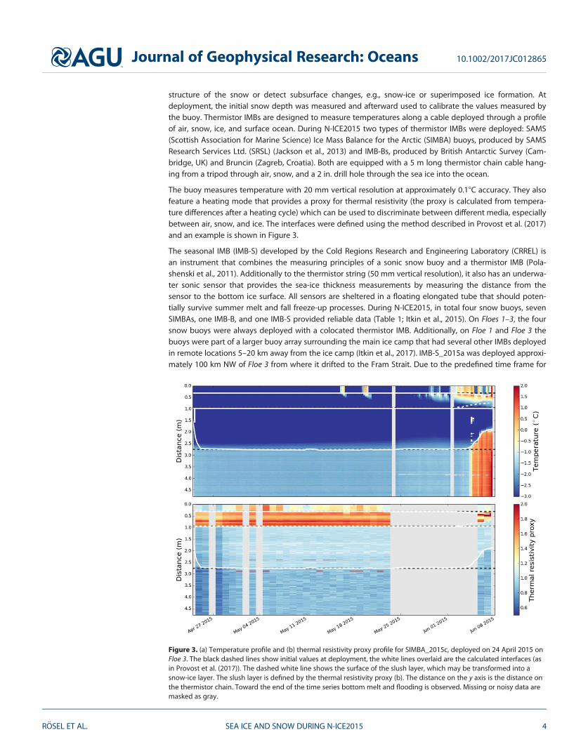
The buoy measures temperature with 20 mm vertical resolution at approximately 0.18C accuracy. They alsofeature a heating mode that provides a proxy for thermal resistivity (the proxy is calculated from tempera-ture differences after a heating cycle) which can be used to discriminate between different media, especiallybetween air, snow, and ice. The interfaces were defined using the method described in Provost et al. (2017)and an example is shown in Figure 3.

The seasonal IMB (IMB-S) developed by the Cold Regions Research and Engineering Laboratory (CRREL) isan instrument that combines the measuring principles of a sonic snow buoy and a thermistor IMB (Pola-shenski et al., 2011). Additionally to the thermistor string (50 mm vertical resolution), it also has an underwa-ter sonic sensor that provides the sea-ice thickness measurements by measuring the distance from thesensor to the bottom ice surface. All sensors are sheltered in a floating elongated tube that should poten-tially survive summer melt and fall freeze-up processes. During N-ICE2015, in total four snow buoys, sevenSIMBAs, one IMB-B, and one IMB-S provided reliable data (Table 1; Itkin et al., 2015). On Floes 1–3, the foursnow buoys were always deployed with a colocated thermistor IMB. Additionally, on Floe 1 and Floe 3 thebuoys were part of a larger buoy array surrounding the main ice camp that had several other IMBs deployedin remote locations 5–20 km away from the ice camp (Itkin et al., 2017). IMB-S_2015a was deployed approxi-mately 100 km NW of Floe 3 from where it drifted to the Fram Strait. Due to the predefined time frame for

Figure 3. (a) Temperature profile and (b) thermal resistivity proxy profile for SIMBA_2015c, deployed on 24 April 2015 onFloe 3. The black dashed lines show initial values at deployment, the white lines overlaid are the calculated interfaces (asin Provost et al. (2017)). The dashed white line shows the surface of the slush layer, which may be transformed into asnow-ice layer. The slush layer is defined by the thermal resistivity proxy (b). The distance on the y axis is the distance onthe thermistor chain. Toward the end of the time series bottom melt and flooding is observed. Missing or noisy data aremasked as gray.



the N-ICE2015 expedition, the duration of Floe 4 was expected to be short and since buoys would not freezeinto the ice after the onset of melt, none were deployed.

3.2. Hotwires and Snow StakesSnow stakes and hotwire fields are commonly used and considered as low cost methods for continuous iceand snow thickness observations and used during, e.g., the SHEBA drift (Mahoney et al., 2009; Perovich,2003). Compared with autonomous buoys they provide snow depth and sea-ice thickness at reduced tem-poral resolution. On the four N-ICE2015 Floes, we installed in total seven hotwire fields and seven snow-stake fields following the routine outlined in Perovich (2003). A rectangular hotwire field with a side lengthof approximately 10 m was designed in a way that in each corner a wire was installed close to an ablation

Table 1Temporal Coverage and Initial Conditions (Measured at Time of Deployment) of IMBs, Snow Buoys, Snow Stakes, and Hotwire Fields Deployed During N-ICE2015 onAll Floes

Instrument Type

Startdate

dd.mm.

Enddate

dd.mm. DaysIce

type

Initialsnow

depth (m)

Initial icethickness

(m)

Meansnow

depth (m)

Meanice

thickness (m)

D Snow(m) per30 days

D Ice(m) per30 days

Floe 1 WAVE_2015b Point 16.01. 23.02. 39 FYIa 0.15 6 0.05 0.82 6 0.09 n/a n/a n/a n/aSIMBA_2015a Point 15.01. 12.03. 57 SYIa 0.59 6 0.09 1.33 0.53 6 0.08 1.26 6 0.12 20.15 20.13SIMBA_2015b Point 15.01. 13.03. 58 SYIa 0.44 6 0.08 1.28 6 0.01 0.39 6 0.04 1.33 6 0.02 0.00 0.00SIMBA_2015e Point 26.01. 23.02. 29 SYIa 0.21 6 0.06 1.49 n/a 1.53 6 0.04 n/a 20.11SIMBA_2015f Point 24.01. 17.02. 25 FYI 0.33 6 0.14 0.90 0.51 6 0.07 0.95 6 0.02 0.10 0.13SIMBA_2015g Point 31.01. 28.02. 29 n/a 0.41 6 0.03 1.08 0.43 6 0.04 1.14 6 0.05 0.02 20.04SNOW_2015a Point 25.01. 21.02. 28 FYI 0.32 6 0.02 0.90 n/a n/a n/a n/aHW1/SS1 Point 23.01. 16.02. 25 FYI 0.55 6 0.13 0.94 6 0.10 0.57 6 0.15 0.95 6 0.09 0.13 0.05HW2/SS2 Point 27.01. 16.02. 21 FYI 0.22 6 0.04 0.94 6 0.04 0.28 6 0.10 n/a 0.20 n/aHW3 Point 27.01. 16.02. 21 YI 0.02 0.41 6 0.14 n/a 0.56 6 0.10 n/a 0.23HW4/SS4 Point 27.01. 16.02. 21 SYI 0.36 6 0.11 1.29 6 0.05 0.43 6 0.04 1.29 6 0.01 0.10 0.00EM31/MP Line i 15.01. 17.02. 34 Mixed n/a n/a 0.41 6 0.19 1.47 6 0.63 n/a n/aEM31/MP Line r 24.01. 15.02. 23 FYI 0.30 0.97 0.33 6 0.14 0.99 6 0.29 0.04 0.08EM31/MP Line r 24.01. 15.02. 23 SYI 0.49 1.7 0.52 6 0.12 1.73 6 0.57 0.08 0.11Average Floe 1 0.34 6 0.16 1.08 6 0.33 0.44 6 0.10 1.20 6 0.33

Floe 2 SIMBA_2015d Point 07.03. 25.04. 49 SYI 0.42 1.30 0.43 6 0.03 1.26 6 0.02 20.02 0.02SNOW_2015d Point 01.03. 25.04. 55 SYI 0.34 1.34 0.41 6 0.03 n/a 0.04 n/aEM31/MP Line i 24.02. 19.03. 24 Mixed n/a n/a 0.56 6 0.17 1.21 6 0.87 n/a n/aEM31/MP Line r 26.02. 09.03. 14 Mixed 0.52 1.44 0.54 6 0.19 1.23 6 0.79 0.03 20.08SS5 Point 02.03. 19.03. 18 SYI 0.36 6 0.04 n/a 0.33 6 0.02 n/a 20.07 n/aSS6 Point 27.02. 17.03. 22 FYI 0.33 6 0.04 n/a 0.37 6 0.03 n/a 0.10 n/aAverage Floe 2 0.40 6 0.08 1.36 6 0.07 0.44 6 0.09 1.23 6 0.03

Floe 3 SIMBA_2015c Point 24.04. 07.06. 45 SYI 0.61 1.79 0.60 6 0.08 1.77 6 0.11 20.23 20.38SNOW_2015b Point 23.04. 07.06. 45 SYI 0.42 n/a 0.47 6 0.02 n/a n/a n/aIMB-B_2015b Point 08.05. 11.06. 36 YI 0.02 0.62 n/a 0.50 6 0.10 n/a 20.47IMB-S_2015a Point 19.05. 06.07.c FYI 0.28 1.05 n/a n/a n/a n/aSNOW_2015c Point 20.04. 11.06. 53 n/a 0.33 1.25 0.35 6 0.03 n/a 20.01 n/aSNOW_2015e Point 21.04. 11.06. 54 n/a 0.32 1.34 0.39 6 0.02 n/a 0.04 n/aEM31/MP Line i 18.04. 05.06. 49 Mixed n/a n/a 0.43 6 0.24 1.45 6 0.82 n/a n/aEM31/MP Line r 27.04. 04.06. 42 Mixed 0.57 1.43 0.53 6 0.17 1.56 6 0.51 20.03 20.06HW7/SS7 Point 29.04. 04.06. 37 SYI 0.55 6 0.17 1.47 6 0.11 0.55 6 0.01 1.45 6 0.05 0.02 20.10HW8/SS8 Point 04.05. 31.05. 28 SYIa 0.70 6 0.10 1.08 6 0.17 0.70 6 0.01 1.05 6 0.03 20.01 20.08Average Floe 3 0.42 6 0.21 1.27 6 0.33 0.50 6 0.12 1.30 6 0.4

Floe 4 EM3/MP1 Line i 10.06. 18.06. 9 Mixed n/a n/a 0.29 6 0.18 1.19 6 0.52 n/a n/aEM31/MP Line r 11.06. 16.06. 6 Mixed n/a n/a 0.32 6 0.20 1.36 6 0.76 n/a n/aHW9 Point 08.06. 18.06. 11 FYIb n/a 1.74 6 0.04 n/a 1.33 6 0.41 n/a 22.37Average Floe 4 1.74 6 0.04 0.31 6 0.02 1.29 6 0.09

Note. For sampling with EM31/Magnaprobe (MP), mean thickness is calculated from EM31 measurements, subtracted by snow depth (description in the text)and shown with standard deviation over the given period. Note that standard deviations for point measurements are temporal while they are spatial for linemeasurements. Line i stands for independent measurements, line r stand for repeated transect lines. The difference (D) is calculated from the first and the lasttransects on a floe and normalized to a 30 day period to make numbers intercomparable.

aIce type is an estimation, derived from initial snow and ice thicknesses.bLikely deformed ice.cLast date where snow and ice data was transmitted, the buoy drifted into Fram Strait until 12 September 2015.



stake, and in the middle of the hotwire field nine snow stakes with even spacing were set up (Figure 4).Snow depth and ice thickness changes were recorded on a regular basis, and the readings were averagedin space to cover small scale spatial variability (R€osel et al., 2016a, 2016b).

3.3. Spatial Surveys of Snow and Ice Thickness3.3.1. Ground-Based Electromagnetic SurveysTotal ice and snow thickness was measured with portable electromagnetic instruments (EM31 and EM31SH,Geonics Ltd., Mississauga, Ontario, Canada) mounted on a sledge. The EM31s measure the received second-ary electromagnetic field, induced by highly conductive seawater (Kovacs & Morey, 1991). Conductivity val-ues are calibrated with drill hole measurements and postprocessed according to Haas et al. (1997). In total101 and 145, calibration drillings were made for EM31SH and EM31, respectively, covering a thickness rangefrom 0.15 to 4.50 m. Analysis of the calibration measurements did not reveal any drift in the fitting curveparameters on the temporal or spatial scales (see supporting information Figure S1).

The footprint size of the EM31 ranges from 3 to 5 m (e.g., Haas et al., 1997; Renner et al., 2014), dependingon the ice and snow thickness. Accuracy of EM31 measurements is in the range of 60.1 m (Haas et al.,2009) for level ice, becoming higher for rough and deformed ice.

On all Floes, independent (i) and repeated (r) transects with combined EM31 and snow depth measure-ments were performed. Repeated transects are considered as repetitions of marked tracks on a weekly basisto observe temporal change, while independent transects are long surveys in different directions from themain ice camp are to cover the spatial variability of the surrounding area. One repeated transect line mea-surement, typically the first survey, is included in the independent data set.3.3.2. Airborne SurveysHelicopter-borne EM instruments (HEM) (Ferra Dynamics Inc., Mississauga, Ontario, Canada) were used tomeasure ice thickness in helicopter range around RV Lance between 15 April and 8 June 2015. Altogether,17 HEM surveys were undertaken. The first, on 15 April, occurred while RV Lance was traveling into the iceto begin the drift of Floe 3. Sixteen surveys were carried out between 19 April and 18 May while RV Lancewas moored to Floe 3. The last survey on 8 June 2015 was an overflight of Floe 4, operated from the FS Polar-stern’s expedition ‘‘PS92’’ (ARK-XXIX/1, Alfred-Wegener Institute (AWI), Bremerhaven, Germany; Peeken,2015).

HEM measurements use the same principle as the EM31 ground surveys: They both measure the distancefrom the instrument to the ice bottom. The HEM uses additionally a laser altimeter to measure the heightabove the snow surface. The laser footprint has a diameter of about 3 cm.

The height above the bottom of the ice is derived from the strength of electromagnetic induction in theconductive water under the ice, and the height of the instrument above the surface of the ice or snow isdetermined with a laser altimeter (Haas et al., 2009, 2010). The difference between the two height measure-ments corresponds to the total thickness of ice and snow. The HEM instruments used in this study have hor-izontal coplaner transmitting and receiving coils spaced 2.7 m apart. They operate at a signal frequency of4 kHz, with a 10 Hz sampling rate, corresponding to measurement point spacing of 3–5 m (Haas et al., 2009;Pfaffhuber et al., 2012). The HEM instrument is flown at a height of 15–20 m above the surface and has a

Figure 4. (a and b) Photo and schematic of a combined hotwire and snow-stake field: red squares are the positions of hotwires, blue circle is the grounding wire.Black squares show the nine snow stakes. (c) Schematic of a hotwire and the grounding wire, connected prior to the measurement to a generator.



footprint of approximately 40–50 m (Haas et al., 2009). The system is calibrated by measuring at high eleva-tions and over open water. The nominal total thickness uncertainty for a single HEM measurement is 0.1 mover level ice, with significantly larger errors and an underestimation of maximum thickness occurring inheavily ridged areas due to footprint smoothing (Haas et al., 2009; Mahoney et al., 2015).

3.4. Snow Depth SurveysSnow depth surveys were made with a GPS snow probe, henceforth referred to as Magnaprobe (Snow-Hydro, Fairbanks, AK, USA). The Magnaprobe is a thin pole with a sliding disk of 0.2 m in diameter around it.The pole penetrates the snow pack to the sea-ice surface while the disk rests on the snow surface. Insidethe pole a magnetic device measures the distance between the disk and the lower tip of the pole providingthe snow depth (Sturm & Holmgren, 1999). Each depth is time-tagged and position-tagged and recordedon a data logger. The Magnaprobe enables snow depth surveys with several thousand snow depth meas-urements in a few hours. The accuracy of the measurement is 63 mm (Marshall et al., 2006) and the foot-print is the size of the disk.

3.5. Merging of Electromagnetic Soundings and Magnaprobe MeasurementsFor direct comparison of the values, and to subtract the snow depth from the EM31 data, we resampled theEM31 data onto the coordinates of the Magnaprobe track, and we applied a Gaussian filter to the EM31data. The EM31 and Magnaprobe data sets (R€osel et al., 2016c, 2016d) were median-sampled on a 5 m regu-lar grid, following the approach by Geiger et al. (2015). Snow depth was subtracted from the EM31 valuesto derive sea-ice thickness. To facilitate this regridding, both the Magnaprobe and EM31 data were cor-rected for sea-ice drift. The drift correction routine is based on subtraction of the floe track over the periodpreceding the exact timing the measurement was carried out. Starting from the second position of theinstrument in the particular measurement sequence, the Global Navigation Satellite System (GNSS) stationcoordinates were used to calculate the back trajectories of the measurement points with respect to initialtime of the series.

The floe track itself is computed using the data from one of two GNSS base stations (called hereafter GPS1and GPS2) that were installed on the ice stations, or the Lance position when the base stations were not inoperation. Note the approach we use implicitly assumes that rotation of the floe over the measurementperiod was negligible. This is reasonable since EM31 and Magnaprobe measurements were always carriedout at the same time with a maximal time lag of 30 s. The single point horizontal accuracy for such floe posi-tion measurements varies in time being of the order of 1–4 m. For those measurements, where single pointaccuracy was critical, such as, e.g., validation fields for airborne campaigns, the data were postprocessedusing Precise Point Positioning (PPP) processed reference tracks of GPS1 and GPS2. This increases the trackaccuracy to 0.2–0.3 m and takes the rotation of the floes into account. The PPP processing was performedby using the open source RTKLIB software package (http://www.rtklib.com).

In order to avoid oversampling for the survey periods when the instrument was stationary relative to theice, we estimated the instrument velocity from the drift corrected measurement positions and eliminatedthe values corresponding to instrument speeds below 0.2 m s21.

3.6. Drill Hole Measurements and Freeboard Calculations3.6.1. Drill Hole MeasurementsDuring the N-ICE2015 expedition, we obtained more than 400 direct measurements from drill holes or holesfrom ice coring on different types of level ice. They are arbitrarily located in the vicinity of the snow and icethickness transects, within a 5 km radius around the ship. For measuring freeboard at the drill holes, firstsnow thickness is measured above the drill hole, afterward snow is removed and the hole is directly drilledor cored into the sea ice. The thickness is measured with a flexible thickness gauge with a foldable metalpiece at the bottom as weight. The distances from the ocean-ice interface to both the water surface andthe ice surface are noted. We estimate the uncertainty of these measurements to be less than 60.02 m,resulting from the sampling uncertainties such as, i.e., different observers, differences in reading of thetape, different strength of pulling the tape, or uneven bottom of the sea ice. More than half of the thicknessdrillings are used for the calibration of electromagnetic measurements (see section 3.3.1). Drill hole meas-urements provide spatial ice and snow thickness as well as freeboard and draft information at point scale,but without temporal component (R€osel & King, 2017).



http://www.rtklib.com

3.6.2. Freeboard CalculationsFreeboard values hfb can either be read directly from tape measurements at drill holes, or they can be calcu-lated based on the principle of an isostatic equilibrium (Forsstr€om et al., 2011):

hi5qw

qw2qihfb1

qs

qw2qihs (1)

where qw is 1,027 kg m23 (Meyer et al., 2017b). For winter conditions (Floe 1 and Floe 2), the bulk density ofthe snow pack is qs 5 345 6 39 kg m23, bulk density for FYI is qi 5 910 6 18 kg m23. For spring conditions(Floe 3 and Floe 4) we define qs 5 313 6 50 kg m23 and qi 5 901 6 18 kg m23; density values are extractedfrom snow pits (Gallet et al., 2017; Merkouriadi et al., 2017b) and ice core analysis (Gerland et al., 2017). Forsnow depth hs, we used Magnaprobe measurements and for ice thickness hi , we used the values obtainedfrom the combination of EM31 and Magnaprobe data. In this study, we analyze calculated freeboard fromlong independent walks. By using equation (1) we have to take into account that we might get results withan offset toward higher freeboard values in case of flooding, because qs of a flooded snow pack will be sub-stantially higher.

4. Results

The combined sea ice and snow thickness data from all different sources is summarized in Table 1, provid-ing an overview about the temporal and spatial variability of snow and ice thickness during the entire N-ICE2015 expedition.

Independent snow and ice thickness transects from combined EM31/Magnaprobe measurements give aver-age values, including standard deviations, in the range from 1.19 6 0.52 to 1.47 6 0.63 m for ice and0.29 6 0.18 to 0.56 6 0.17 m for snow, for all the floes (Table 1). Average values of ice and snow thicknessfrom point measurements and their evolution throughout the entire N-ICE2015 expedition from January toJune 2015 are shown in Figure 5.

Figure 5. (a) Snow depth and (b) sea-ice thickness, extracted from IMBs, snow buoys, snow-stake fields (SS), and hotwirefields (HW) during N-ICE2015. The error bars represent the standard deviations. The purple shading in the backgroundindicates storm events, labeled as M (major) and m (minor) storms according to Cohen et al. (2017). The stars show majorsnow fall events (Cohen et al., 2017). Note that before 2 February 2015 no precipitation data, and between 18 March and18 April 2015 no wind speed and no precipitation data are available.



4.1. Floe 1: 15 January to 21 February 2015The data acquired by five IMBs, a snow buoy, hotwire, and snow-stake fields associated with Floe 1 and itssurrounding represent different snow and ice conditions observed during the drift. All buoys show a weakincrease in ice thickness during a period of low air temperatures in the last week of January, followed by anincrease of snow depth from 0.59 to 0.66 m for SIMBA_2015a and a decrease from 0.45 to 0.35 m for SIM-BA_2015b (Itkin et al., 2015). During a major storm event lasting from 3 to 8 February (M2) (Cohen et al.,2017), snow depth at SIMBA_2015b and SIMBA_2015g decreased, while it increased at SIMBA_2015e. SIM-BA_2015a, SIMBA_2015f, and SIMBA_2015g show both: first an increase and later a decrease of snow depth(Figure 5). The decrease in snow depth can be explained by blowing snow and its redistribution. It shouldbe noted that these are point measurements and they do not capture the spatial variability of the snow.

While drifting over Atlantic Water in mid-February (Meyer et al., 2017b) the southernmost buoy SIMBA_2015a(20 km distant from Floe 1) indicates bottom melt starting on 16 February, followed by a similar signal fromSIMBA_2015e and SIMBA_2015g starting on 19 February (Figure 5). Initial flooding with a gradual snow-iceformation on the snow/ice interface was observed at SIMBA_2015a (Figure 5; Provost et al., 2017). Due to icetemperatures of 24.58C we surmise that the ice was permeable (Weeks & Ackley, 1986), and negative free-board promoted snow-ice formation on SIMBA_2015a. During the last week of February and the first week ofMarch, ice breakup events, flooding, and subsequent snow-ice formation led to a rapid decrease of snowdepth and an increase of ice thickness. On 18 February, a deformation event led to lateral flooding of Floe 1,and subsequent snow-ice formation was observed in the SIMBA_2015f record (Provost et al., 2017).

From the hotwire and snow-stake fields HW1&SS1 (FYI) and HW4&SS4 (SYI) initial ice thicknesses with stan-dard deviations were 0.94 6 0.1, and 1.29 6 0.05 m, respectively (Table 1). The last readings 4 weeks latershowed values of 0.98 6 0.06, and 1.30 6 0.05 m, respectively. Only hotwire field HW3, deployed in a refro-zen lead with an initial snow cover of 0.02 m showed a significant increase from 0.41 6 0.14 to0.64 6 0.09 m (Table 1 and Figure 5). The initial snow depth with standard deviation at the SYI field was0.55 6 0.13 m, and about 0.16 m higher than at the FYI field with an initial observed snow depth of0.39 6 0.11 m. On both ice types the snow depth showed a net increase of about 0.1 m within 1 month.

Figure 6a presents Floe 1 ice and snow thickness probability density functions (PDF) derived from indepen-dent measurements with EM31 and Magnaprobe. Note, that in Figure 6, all distributions represent both spa-tial and temporal variability since spatial data from a longer period are included. The PDF of the icethickness features a trimodal distribution with a first peak at 0.3 m corresponding to thin ice, a second peakat 0.9 m, and a third major peak, which represents the primary mode at 1.5 m. Mean ice thickness was1.47 m with a standard deviation of 0.63 m. The tail of the PDF above 1.8 m represents deformed ice.

The modal ice thickness for all repeated FYI transects was 0.80 m (Figure 6b). The modal thickness for allrepeated SYI transects was 1.40 m. On FYI, the average snow depth with standard deviation was0.33 6 0.14 m, whereas on SYI, it was 0.52 6 0.14 m (Figure 6b). The distributions of both snow depth andice thickness do not differ greatly over either type between the first and last transect lines. We notice a shiftfrom the FYI mode from 0.8 to 0.9 m and for the SYI mode from 1.5 to 1.6 m, but the averages for both icetypes for the first and the last transect stayed in the same order of 1 m for FYI and 1.8 m for SYI. The modefor snow thickness on FYI increased by 0.05 m from 0.20 to 0.25 m on FYI while it decreased by the sameamount from 0.60 to 0.55 m on SYI.

4.2. Floe 2: 24 February to 19 March 2015On Floe 2, snow buoy SNOW_2015d, SIMBA_2015d, and snow-stake field SS5 were deployed together on SYI atthe main ice camp. Initial snow depth for SNOW_2015d was 0.34 m (Table 1). The buoy showed an increase of0.15 m in snow depth after deployment, caused by two major storm events (M4 and M5) with precipitation(Cohen et al., 2017). SIMBA_2015d was deployed 1 week later, after the storm, with initial snow and ice thick-nesses of 0.42 and 1.30 m, respectively. During the drift, we registered only slight variations in the range of a fewcentimeters in snow depth and ice thickness (Figure 5). The snow-stake field on FYI (SS6) showed an increasefrom 0.33 to 0.41 m while the snow stakes on SYI (SS5) showed a decrease from 0.36 to 0.32 m (Figure 5).

The thickness distributions for the independent measurements and the repeated transect lines (Figures 6dand 6e) on Floe 2 show similarities: the thin ice class with ice thickness values in the range from 0.0 to 0.3 mis present in both histograms. The main modal peak is around 1.0 m, representing the fraction of



dominating FYI. For the transect lines, a third mode can be identified at 1.3 m, whereas in the independentmeasurements, a third mode is at 1.8 m. The snow depth with standard deviation on Floe 2 from indepen-dent measurement is comparable to the measurements on the transect line and the mean is 0.55 6 0.18 m(Figure 6d). On Floe 2, the conditions were quite stable; the average thickness of ice and snow did notchange within 3 weeks of the drift on this floe (Table 1). Snow depth on FYI and SYI was in the range of0.33–0.56 m (Table 1), but it is not distinct that the values in the higher range always correspond with SYI.

4.3. Floe 3: 18 April to 5 June 2015The IMBs, snow-stake, and hotwire fields on Floe 3 show coinciding results throughout the drift. During thefirst 4 weeks after the installation of the snow-stake and hotwire sea-ice and snow conditions remained

Figure 6. Snow and ice thickness distributions from (left) independent measurements and (middle) repeated measure-ments for all Floes. SYI and FYI is only distinguished for Floe 1 on all repeated transects, for Floes 2, 3, and 4 the distribu-tions contain a mixture of SYI and FYI. The right column displays calculated freeboard from the independentmeasurements of each floe. The gray shaded areas indicate the values that fall in the uncertainty range of 60.06 m basedon 61 STD. The bins in the pdfs are centered and bin size for ice thickness is 0.10 m, for snow depth 0.05 m, for freeboard0.01 m. All distributions represent both spatial and temporal variability.



stable around 1.08 and on 1.47 m on SYI with 0.70 and 0.55 m of snow. This is confirmed by the data fromSIMBA_2015c, which had an initial ice thickness of 1.79 m with 0.61 m snow. Starting at the beginning ofJune, rapid bottom melt with a rate of about 0.10 m d21 commenced on both ice types, while the snowdepth remained unchanged. SIMBA_2015c shows an indication of a weak basal melt already after 25 Mayfollowed by a steep increase of the basal melt rate on 5 June (Figure 3). Subsequent freeboard adjustmentand flooding of the floe caused the formation of a slush layer with a thickness of up to 0.30 m (Figure 3).Due to the high density and the salinity of the slush layer and its potential to refreeze, we will here considerthe slush layer as sea ice. Observed 2 m air temperatures well below 08C until 1 June (Hudson et al., 2015)and also cold sea-ice temperatures may allow the slush layer to refreeze subsequently to a snow-ice layer.Consequently, snow depth measured by SIMBA_2015c gradually decreased, starting at the end of May. Thenext significant decrease in snow depth registered in early June by the three snow buoys is connected tostorm events (Figure 5: M8 on 2–6 June and m9 on 8 June; Cohen et al., 2017), and might be caused by lat-eral flooding induced by breakup events of Floe 3. Note, that snow buoys can only measure the change ofthe distance from the snow surface to the sensor, which was in this case an increase and might be a sign ofcompacting snow. Flooding or snow-ice formation cannot be detected by snow buoys. IMB-B_2015b wasdeployed on 8 May in a refrozen lead about 20 km NW of RV Lance with initial ice thickness of 0.62 and0.02 m of snow. This is below the detection limit of the thermistor chain, so no snow depth can be shownin Figure 5. A gentle decrease of ice thickness from the bottom can be observed already after 16 May, fol-lowed by a sharp increase of the basal melt rate on 5 June that continued until complete disintegration ofthe level ice on 12 June, 20 km from the open water (Figure 5). IMB-S_2015a was deployed on 19 May onlevel FYI with initial thicknesses of 1.05 m for ice and 0.28 m for snow, respectively. IMB-S_2015a showed nosign of snow-ice formation. Ice and snow thickness both decrease gradually in June, caused by bottommelting and snow melt or compaction.

The repeated measurements on Floe 3 also showed stable conditions in terms of snow and ice thicknessuntil the onset of gradual melt in the second half of May. Then both snow and ice thickness show adecrease in thickness (see Table 1). The comparison of the first and the last repeated transect line results inan average decrease of 0.16 m in ice thickness and 0.02 m in snow thickness. The sea-ice thickness distribu-tion of Floe 3 is bimodal, with a first mode at 1.2 m and a second mode at 0.2 m, which represents a largerefrozen lead in the vicinity of the ship (Figure 6g). Connected to these two distinct sea-ice modes, theobserved snow depth distribution shows a peak at 0.03 m representing the snow cover of the refrozenlead. The second mode is at 0.45 m associated with the snow cover on FYI and SYI. Figures 6g and 6h dem-onstrate that the distributions from the independent measurements and the repeated transect lines arecomparable, except for the mode corresponding to the snow on thin ice only present in the independentmeasurements.

4.4. Floe 4: 7 to 22 June 2015Floe 4 was established on FYI within the marginal ice zone. At the hotwire field HW9, an intense bottommelting event was observed, which started between 10 and 13 June, with melt rates up to 0.25 m d21 (Fig-ure 5). This hotwire field was in a deformed area of the floe, therefore may not be fully representative ofprocesses on level ice. We assume the ocean induced melting of deformed ice could lead to disintegrationof previously consolidated ice blocks efficiently accelerating the melt process.

The snow and ice distributions for Floe 4 both show an unimodal distribution, where the mode for snow islocated at 0.20 m and for ice at 1.25 m (Figures 6j and 6k). The comparison of independent measurementswith repeated transects shows that the transect lines represent well the overall surrounding (Table 1). OnFloe 4, the established survey line could not be followed due to strong bottom melt and a rapid transitionfrom solid into rotten ice, making a quantitative intercomparison of the entire surveys difficult. However,we found a decrease of the average sea-ice thickness of 0.5 m within 10 days when we compare the firstand the last transect line. This might also explain the wider thickness distributions for Floe 4. The snowthickness decreased by 0.05 m. In general, a flooding of vast parts of Floe 4 was registered after 14 June,along with formation of a snow-ice crust in wet snow (see Figure 7) above the flooded snow pack. This icelayer grew over several days toward the former snow/ice interface. The formation of this crust resulted in asudden decrease of snow depth and the same amount of increase in ice thickness; we noted that in manyareas the Magnaprobe pole could not penetrate through the crust to the original snow/ice interface andmight bias the observations.



4.5. Regional HEM Surveys Over Floe 3 and Floe 4 SurroundingsFigure 8 presents all HEM surveys including date and time (King et al., 2016); basic statistics for each surveyare summarized in Table 2. The total snow and ice thickness distribution for all HEM surveys combined hasmode 1.7 m and mean 1.8 m. There is a second mode at between 0.1 and 0.3 m in almost all the surveysthat is representative of the thin ice class found in refrozen leads.

Long HEM surveys toward the east on 6 and 12 May show a distribution dominated by the thin ice class,while flights along the main drift direction show very little variation between the surveys.

Figure 7. Snow pits with flooded snow pack on Floe 4 on 14 June 2015 on three different sites. (a) Close to the ship, waterlevel at 0.075 m, wet snow until 0.14 m, total snow depth 0.30 m. (b) Water level at 0.13 m, wet snow until 0.19 m, totalsnow depth 0.53 m. (c) Water level at 0.06 m, wet snow until 0.09 m, total snow depth 0.34 m.

Figure 8. HEM surveys carried out in the N-ICE region between 15 April and 8 June 2015. The flight at 828N/208E was areconnaissance flight on the way the start position of the third drift. The background is sea-ice concentration (black is 0%;white is 100% sea-ice concentration) from 15 May 2015 based on SSM/I data, calculated with ASI algorithm, provided byICDC, University Hamburg.



Four local area surveys with a radius of 10 km around the ice stationwere carried out on a repeated pattern over RV Lance’s position on 24and 28 April and on 5 and 11 May. Between the 28 April and 5 May anincrease of the second mode from 0.1 to 0.2 m can be observed, indi-cating a thickening of the YI. The primary mode ranges between 1.7and 1.8 m. The local survey on 11 May did not follow exactly the pat-tern of the previous three surveys due to bad weather. The ice thick-ness distribution of this flight has a primary mode at 1.5 m and aweak second mode at 0.3 m.

The HEM flight on 8 June over Floe 4 shows a slightly thinner sea-icecover with a mode at 1.4 m and a mean thickness of 1.5 m.

4.6. Comparing Airborne With Ground-Based EM DataThe independent EM31 data set agrees well with HEM measurements inthe vicinity of Floe 3 made from mid-April until mid-May (Figure 9a).Both PDFs show a bimodal distribution with the major peak in thethicker level ice, and a second mode, representing the thin ice. The thinice mode is less pronounced in the EM31 data, because for safety rea-sons it was difficult to collect data of ice thickness in newly refrozenleads. This under-representation of very thin ice also explains the slightlyhigher mean values of ice thickness derived from the EM31 data.

As strong bottom melting resulted in a remarkable thinning on Floe 4 onlytwo EM31 surveys on 10 and 11 June can be compared with the HEM sur-vey from 8 June. The modes for both distributions are at 1.3 m, the meanfor EM31 is 1.7 m, and for HEM 1.5 m (Figure 9b). On Floe 4, no thin ice orrefrozen lead was present in the area of the ice station, but in the largervicinity, which was covered by the HEM survey on 8 June (Figure 9b).

4.7. Freeboard During N-ICE2015On all four floes widespread negative freeboard along with floodedareas was observed from the drilling records: 32% (Floe 1), 37% (Floe

Table 2Total Snow and Ice Thickness From HEM Surveys

Date Start lon/lat Thickness mode (m) Thickness mean (m) Notes

15 Apr 2015 19.81/81.95 1.9 (0.1) 1.8 6 0.9 Reconnaissance flight19 Apr 2015 14.26/83.15 1.8 2.1 6 0.824 Apr 2015 15.37/82.75 1.7 (0.1) 1.7 6 0.8 Local area survey24 Apr 2015 15.30/82.73 1.7 (0.3) 1.8 6 1.028 Apr 2015 13.96/82.18 1.8 (0.1) 1.8 6 0.9 Local area survey29 Apr 2015 13.57/82.07 1.5 1.9 6 1.030 Apr 2015 13.30/82.00 1.9 (0.2) 2.1 6 1.105 May 2015 13.20/81.80 1.7 (0.2) 1.6 6 0.9 Local area survey05 May 2015 13.43/81.79 1.7 (0.3) 1.9 6 0.905 May 2015 13.23/81.77 1.8 (0.2) 1.9 6 1.006 May 2015 13.32/81.76 1.8 (0.1) 1.9 6 1.006 May 2015 13.13/81.79 0.1 (1.8) 1.4 6 1.0 Long track east08 May 2015 12.03/81.63 1.7 (0.1) 1.7 6 1.111 May 2015 9.85/81.40 1.5 (0.3) 1.8 6 0.812 May 2015 9.53/81.36 0.3 (1.3) 1.4 6 1.0 Local area survey/buoy overflight18 May 2015 9.61/81.28 2.0 (0.1) 1.6 6 1.1 Long track south-east08 Jun 2015 19.30/81.10 1.4 (0.1) 1.5 6 0.9All flights 1.7 (0.1) 1.8 6 0.9

Note. Times are UTC. Second mode in brackets is included where one exists. Mode and mean thickness with standarddeviation for all surveys from Floe 3 and Floe 4 are calculated from all of the data points.

Figure 9. (a) Probability density functions of all independent EM31 and HEMice and snow thickness measurements during Floe 3 (April–early June 2015).Average ice thickness from buoys SIMBA_2015c and IMB-B_2015b are markedby a black line. (b) Probability density functions of independent EM31 and HEMice and snow thickness measurements from AWI flight on 8 June 2015 overFloe 4.



2), 61% (Floe 3), and 48% (Floe 4) of the readings show negative free-board, considering an uncertainty of 60.02 m for the measured free-board. All values within this range (in total 31%) were discarded. Weconsider the drill holes to be representative for the area, because theyare numerous (N 5 475) and arbitrarily located. In addition, we havecalculated freeboard from snow and ice thickness measurements ofthe long independent walks referring to the method in section 3.6.2(Figures 6c, 6f, 6i, and 6l). Considering an uncertainty of 60.06 m, thecalculated negative fraction of freeboard on all four floes is 5% onFloe 1, 62% on Floe 2, 18% on Floe 3, and 11% on Floe 4 (Figure 6).

We estimate the uncertainty of the calculated freeboard resultingfrom the propagation of uncertainties in the snow and ice densitiesand the sampling uncertainty (represented by the spatial variability)to be on average 60.06 m. For calculated freeboard considered as afunction of hi, hs, qi , and qs , at every analyzed location, the freeboardabsolute uncertainty is calculated as a square root of the sum ofsquared partial increments of this function due to errors in the inputvariables. We used as measurement error the standard deviations ofqi , and qs , and for hi and hs we used their observed standard devia-tions, since the sampling uncertainty, represented here by the stan-dard deviation of snow and ice measurements, is a betterapproximation of the large areal impact on freeboard than the mea-surement error of each individual point. We consider the errors in thefour measured variables of the error propagation method to be inde-pendent, because they were derived by different methods. The com-parison of observed freeboard to calculated freeboard from drill hole

measurements (Figure 10) gives an overall agreement with a correlation of r2 5 0.49, but it also shows sig-nificant scatter. With regard of the uncertainty of 60.02 m for the measured freeboard, 40% of the drill holevalues lie above the uncertainty, 29% lie below and 31% of the values fall within the range of uncertainty.For the calculated freeboard, a 73% of the values from the independent long walks lie within the uncer-tainty range of 60.06 m, while only 5% lie below and 22% lie above.

It is also noticeable that the correlation is higher for a positive freeboard than for negative freeboard. Thescatter might be caused by the fact that individual locations for the drill holes are not always at isostaticequilibrium since internal pressure in the ice might cause a certain disturbance. In addition, the calculationsappear to underestimate negative freeboard, where the snow load can cause flooding of the snow layerwhich results in a higher density of the snow pack. Additionally, the measurement error for negative free-board values might be higher because the interfaces, especially for water and snow are difficult to distin-guish after flooding.

4.8. Snow Melt on Floe 3 and Floe 4Events of snow melt were observed on both Floe 3 and Floe 4. Temperatures rose to 08C twice in May, butwe observed no change in the snow depth in connection with these events. The onset of intense snowmelt on Floe 3 was registered on 4 June when the 2 m air temperature exceeded 08C and stayed around thefreezing point with slight variations due to the diurnal cycle (Cohen et al., 2017; Hudson et al., 2015).

On Floe 4, we observed a darkening of the snow cover in depressions in the vicinity of pressure ridges on8 June, which was an indication of a continuous wetting of the snow pack. Air temperature remained abovefreezing between 8 and 9 June promoting melt pond formation in these dark spots. Air temperaturedropped again below 08C on 10 June. Distinct signs of snow surface melting due to radiative forcing with arapid transformation of the crystal structure of the snow pack on a large scale was observed on 14 June,when the 2 m air temperature increased again to 08C (Gallet et al., 2017). Additionally, snow pit and ice coretemperature data gave evidence of an isothermal temperature profile through the entire snow and icepack, along with increasing bulk snow densities (Gallet et al., 2017; Gerland et al., 2017; Merkouriadi et al.,2017b).

Figure 10. Scatterplot of freeboard measured in situ at drill holes (R€osel & King,2017) versus the calculated freeboard using equation (1) for all four floes. Theuncertainties based on 61 STD of 60.02 m for measured freeboard and60.06 m for calculated freeboard around 0.0 m are shaded light gray.



5. Discussion

This compilation of the N-ICE2015 snow and sea-ice thickness data sets (R€osel et al., 2016a, 2016b, 2016c,2016d) represents a unique opportunity to study and understand processes in the winter-to-spring evolu-tion of a thinner sea-ice cover with a thick snow cover from the Atlantic sector of the Arctic from winter con-ditions to melt onset.

5.1. Sea Ice During N-ICE2015The N-ICE2015 expedition took place over the Nansen Basin and the Yermak Plateau, in an area where theArctic Ocean is connected to the Atlantic Ocean via the deep Fram Strait and the shallow Barents Sea(Meyer et al., 2017b). The exchange of northward flowing warm and saline Atlantic Water and southwardcold Arctic water near the surface gives in combination with the bathymetry makes this region special interms of heat exchange. The shallow Yermak Plateau is a local hot-spot for vertical mixing and cooling ofAtlantic Water, while in the deep Nansen Basin the cold Polar Water dominates (Meyer et al., 2017b). Also,the Atlantic Ocean and the Fram Strait is a prominent pathway for low pressure systems which penetrateacross the North Pole and cause winter warming events in the Central Arctic (Graham et al., 2017b; Rinkeet al., 2017).

Our observations show that during N-ICE2015, interaction at the ocean-sea-ice interface was determined tobe the most significant factor driving the ice thickness changes, because thick snow moderated the influ-ence from the atmosphere. During winter negative heat fluxes (Meyer et al., 2017a) caused a slight increaseof sea-ice thickness. This increase in thickness was especially pronounced in areas with thin snow cover,e.g., refrozen leads or new ice (Table 1). However, the sea-ice growth is moderated by the insulating effectof the snow cover. The thick snow pack of on average 0.52 6 0.18 m on SYI on Floe 1 in January and Febru-ary, during the coldest period of the experiment, limited thermodynamic ice growth (Provost et al., 2017).When the station drifted over warm Atlantic Water a significant reduction of ice thickness due to bottommelt was observed. In particular, we registered such events once in winter on Floe 1, starting on 17 Februaryat 828N, and twice in spring: on Floe 3, 4–5 June at 808N, and on Floe 4, 12–18 June at 808400N (Meyer et al.,2017a). Both bottom melting events, during Floe 3 and Floe 4 were associated with a strong positive oceanheat flux up to 400 W m22 in the mixed layer at the ocean-ice interface, driven by a combination of shallowAtlantic Water and storm events (Meyer et al., 2017a; Peterson et al., 2017). The combination of positiveocean heat fluxes with storm events or strong swell induced by storm events caused the breakup of theaforementioned floes (Itkin et al., 2017).

From the analysis of multimodal total thickness distributions from EM31 transects on Floe 1 and Floe 2, wecan clearly differentiate between level YI, FYI, SYI, and deformed thick ice. This is, however, not the case onFloe 3, where the modes associated with FYI and SYI are no longer distinct. A similarity in total ice thicknessdistributions for both ice types is also confirmed by the drill hole and ice core measurements. From Floe 3onward, the analysis of total thickness distributions alone is not sufficient for a robust classification of sea-ice types, which then requires, e.g., ice core analysis (Granskog et al., 2017).

5.2. N-ICE2015 in the Context of Other Studies in the RegionIn line with pan-Arctic trends, a shift to a thinner Arctic sea ice during the transition from winter to summerin the last decade in the study region has been already shown in Renner et al. (2013). The comparison ofthe N-ICE2015 HEM surveys with HEM surveys in the same region from April 2009 and April–May 2011(Haas et al., 2010; Renner et al., 2013) revealed a decrease of the mode of total thickness from 2.4 m in 2009over 1.8 m in 2011, down to 1.7 m in 2015. It should be mentioned that most of the N-ICE2015 surveyswere further north than the flights in the previous years at the same time of the year.

Between 838N and 818N no gradient was observed in ice thickness. A gradient toward a thinning of the sea-ice cover occurred from 818N southward. This expected gradient is associated with warm Atlantic Waterinfluence on the ice pack which consequently results in a breakup of floes and rapid melting. According tohistorical observations in the region (e.g., Renner et al., 2013), this process is generally limited to the areawithin a distance of 50 km to open water, which is also shown by the two southernmost HEM flights from12 May and 8 June 2015 having with 1.5 and 1.4 m, respectively, the lowest modal thickness.

Interannual variability of snow and ice thickness is significant on a range of spatial and temporal scales (Fig-ure 11). During N-ICE2015 the observed regional ice thickness was reduced and the snow depth was higher



compared to studies from historical observations (Table 3 and Figure11). For example, the January–February mean snow depth of0.33 6 0.14 m on FYI was higher than the observations during a shorttest cruise prior to N-ICE2015 in February 2014: here the averagesnow depth on FYI was 0.20 6 0.08 on 0.80 m thick sea ice (modalvalue). It is to be noted that the sea ice in this case was most likelyyounger and had thus less snow on top.

The April–May mean snow depth for the same region in 2011,reported in local scale studies of Haapala et al. (2013) and Renneret al. (2013) were 0.36 6 0.26 and 0.32 m, respectively. A 200 m longsnow depth profile from 1 April 2003 on 80.427N, 12.817E duringPolarstern Cruise ARKTIS-IXI/1 resulted in a mean snow depth of0.17 6 0.08 m (Haas, 2018). From the same cruise, average snow andice thicknesses from ice stations were noted with 0.18 6 0.14 and1.96 6 0.43 m, respectively (Sch€unemann & Werner, 2005). During adrifting station with Polarstern on Expedition ARKTIS-IX/1 in March1993 in the same area a 200 m snow and ice thickness profile on2.56 6 0.53 m thick MYI indicated an average snow cover of0.25 6 0.27 m (Table 3 and Figure 11).

While observations from the recent INTPART Field School 2017 cruisein May to the marginal ice zone north of Svalbard showed a significantnumber of floes with snow depths larger than 0.4 m (A. Doulgeriset al., personal communication, 2017), alongside FYI floes with muchless snow. These observations resemble the conditions during N-ICE2015 and give an indication that the situation of thick snow onthin ice could occur more regularly in this region and might favor anincrease in the occurrence of negative freeboard.

In summary, the April to early June mean snow depth of0.50 6 0.12 m averaged over all measurements on Floe 3 (Table 1) wassignificantly higher than the averaged observations of 0.30 6 0.14 mfrom historical observations, including the recent observations from2017 (Table 3).

Compared to the W99 climatology with values of 0.37 m for snowdepth in April in the area north of Svalbard, our observations show

thicker snow. It needs to be noted, however, that the use of W99 in the Atlantic Sector of the Arctic shouldbe treated carefully, since observational data are sparse in this region. In fact, only 41 average snow thick-ness values from the ‘‘Sever’’ Aircraft Landing Observations from the Former Soviet Union from the years1955 and 1975–1979 (Romanov, 2004) are included in W99 for the area north of Svalbard. W99 describes ageneral decadal scale decreasing trend in snow depth between 1954 and 1991, but explained by a decreasemainly in May. In addition, a later onset of ice formation (Johnson & Eicken, 2016; Stroeve et al., 2014) andan associated delay in snow accumulation on sea ice, or liquid precipitation instead of snowfall in theautumn, could lead to a general thinning of the snow cover. Nevertheless, interannual and spatial variabilityof snow thickness is high (Table 3): Forsstr€om et al. (2011) present values in the range of 0.30 6 0.19 m forFram Strait in April–May 2005, 2007, and 2008, while Renner et al. (2014) measure 0.32 6 0.22, 0.47 6 0.24,and 0.39 6 0.22 m for the same years, respectively. It is to be noted that the corresponding sea-ice thick-nesses are also showing high variability in Forsstr€om et al. (2011) and Renner et al. (2014). Fram Strait is con-sidered a region with high drift speeds and the origin of the sea ice might be different than in the areanorth of Svalbard (Spreen et al., 2009).

However, exceptional atmospheric circulation events in autumn 2014 and winter 2015 could have causedthe observed increased snow depth in 2015 in the study area (Merkouriadi et al., 2017a). Studies suggestthat there is evidence, especially for the climate of the Atlantic sector of the Arctic, to shift toward a differ-ent regime with a higher storm frequency and more precipitation events, particularly during the winter

Figure 11. (a) Mean snow thickness, (b) mean sea-ice thickness, and (c) meanand modal total thickness values from historical and recent observations in thearea north of Svalbard, as listed in Table 3. The error bars present the standarddeviation.



season. This can result in an increased snow thickness (Bintanja & Selten, 2014; Graham et al., 2017a;Merkouriadi et al., 2017a; Park et al., 2015).

Based on ERA-Interim reanalysis data along the back trajectories of the four floes for the months Septemberto March over the period 1979–2015, we see that the winter precipitation has increased. The precipitationexperienced by our four floes in winter 2014–2015 lies 50% above the long-term average in our study area(Merkouriadi et al., 2017a). To summarize: in combination with a thinner sea-ice cover (e.g., Hansen et al.,2013; Kwok & Rothrock, 2009) the recently observed amount of snow causes an increase in the snow-iceratio (this will be even the case if the snow depth is not increasing), which favors negative freeboard andsubsequent flooding of the snow pack in the Atlantic sector of the Arctic.

5.3. Thick Snow on Thin Ice Promotes Negative FreeboardOn all four floes widespread negative freeboard along with flooded areas was observed from the drillingrecords (32–61% of the drill holes show negative freeboard). Also the calculated freeboard indicate wide-spread negative freeboard, from 5% (Floe 1) to 62% (Floe 2) of the individual points with snow and ice thick-ness, when an uncertainty of 60.06 m is accounted for Figure 6. Of course, part of the negative freeboardvalues can result from deformation events like ridging, but from the drill hole dataset we have evidencethat negative freeboard was common on level ice. Considering the specific densities of snow and ice, thehydrostatic balance is of snow-covered sea ice with a freeboard of 0 cm is given when the ratio of snowdepth to ice thickness is approximately 1:3 (Sturm & Massom, 2009). Once this ratio is exceeded—either byaccumulating snow on the sea ice or bottom melt of sea ice—and the freeboard becomes negative, lateralflooding or permeation of water through the porous ice with subsequent snow-ice formation can occur.Snow-ice formation is a positive contribution to the sea-ice mass balance and has to be considered in sea-ice models, as snow-ice was found to be widespread during N-ICE2015 (Granskog et al., 2017).

A substantial fraction of areas with negative freeboard can affect regional ice thickness retrievals from satel-lite altimetry data like CryoSat-2 in two ways: (i) a flooded and saline snow pack will raise the main radarscattering horizon, therefore the sea-ice freeboard might be misinterpreted, which results in erroneouslyhigh sea-ice thickness values (Nandan et al., 2017). Further, (ii) areas of negative freeboard might have a dis-proportionately thick snow cover. For CryoSat-2 ice thickness retrieval algorithms, snow depth values fromW99 are widely used, and for FYI dominated regions, it is suggested for calculation of sea-ice thickness to

Table 3Snow and Ice Thickness From Historical and Recent Observations in the Area North of Svalbard During April to Early June

Date ExpeditionMean snowdepth (m)

Mean sea-icethickness (m)

Modal totalthickness (m) Reference

April 1955 ‘‘Sever’’ Aircraft landings 0.16 6 0.16 0.94 6 0.42 n/a Romanov (1996)April 1974 ‘‘Sever’’ Aircraft landings 0.38 6 0.12 2.92 6 0.11 n/a Romanov (1996)April 1975 ‘‘Sever’’ Aircraft landings 0.29 6 0.13 2.28 6 0.49 n/a Romanov (1996)April 1976 ‘‘Sever’’ Aircraft landings 0.46 6 0.08 2.33 6 0.10 n/a Romanov (1996)April 1977 ‘‘Sever’’ Aircraft landings 0.45 6 0.16 2.6 n/a Romanov (1996)April 1978 ‘‘Sever’’ Aircraft landings 0.16 6 0.01 2.75 6 0.35 n/a Romanov (1996)April–May 1979 ‘‘Sever’’ Aircraft landings 0.2 6 0.09 1.93 6 0.65 n/a Romanov (1996)April–May 1954–1991 Climatology 0.37 n/a n/a Warren et al. (1999), N-ICE2015 areaMarch 1993 PS ARKTIS-IX/1 0.25 6 0.27 2.56 6 0.43 n/a Eicken and Meincke (1994)1 April 2003 PS ARKTIS-IXI/1 0.17 6 0.08 n/a n/a Haas (2018)April 2003 PS ARKTIS-IXI/1 0.18 6 0.14 1.96 6 0.43 n/a Sch€unemann and Werner (2005)18 May to 4 June 2005 Fram Strait 0.32 6 0.22 2.5 6 1.1 (total ice and snow) 2.6 6 1.7 Renner et al. (2014)10–30 April 2007 Fram Strait 0.47 6 0.24 2.5 6 0.9 (total ice and snow) n/a Renner et al. (2014)April–May 2005/2007/2008 Fram Strait 0.30 6 0.19 1.88 6 0.83 n/a Forsstr€om et al. (2011)16 April to 1 June 2008 Fram Strait 0.39 6 0.22 3.2 6 1.1 (total ice and snow) 2.7 6 1.6 Renner et al. (2014)April 2009 Polar 5 flight n/a n/a 2.4 Haas et al. (2010)April–May 2011 ICE2011 0.36 6 0.26 n/a 1.8 Haapala et al. (2013)April–May 2011 KVS2011/ICE2011 0.32 n/a 1.8 Renner et al. (2013)February 2014 N-ICE Testcruise 0.20 6 0.08 n/a 0.80 (FYI) Unpublished data, NPIApril–June 2015 N-ICE2015 0.53 6 0.17 1.56 6 0.51 1.7 This paper, Floe 3, EM31/MP(i)May 2017 INTPART Cruise 0.41 6 0.23 1.65 6 0.50 n/a Unpublished data, NPI



use only half of the snow depth given in W99 (e.g., Laxon et al., 2013). For the conditions during N-ICE2015,where the observed snow depth in the area north of Svalbard region was 73% higher than the climatologi-cal value of W99 for the months April and May, this results in an underestimation of the CryoSat-2 sea-icethickness product compared to the ground truth data. As an example, with a freeboard of 0.05 m, the calcu-lated sea-ice thickness for hs 5 0.185 m (which represents the value of W99/2 which is typically applied forthis region), the calculated sea-ice thickness results in 0.87 m for spring conditions (using equation (1)),while with an observed snow thickness of 0.53 m results in an ice thickness of 1.72 m. Another importantpoint to mention in this context is that the presence of thick snow cover might be biased toward higher val-ues in ice thickness (e.g., Kwok, 2014; Ricker et al., 2015). Again, we advise a closer look into the regionalcharacteristics when data are used in a pan-Arctic context, since the observations from the Atlantic sectordiffer substantially from those of the western Arctic.

6. Conclusion

We have presented a comprehensive data set in which ground-based point measurements from buoys,snow stakes, or drill holes, are complemented by local scale surveys of ice and snow thickness with EM31and Magnaprobe, and more regional observations with airborne instruments. The N-ICE2015 expeditiontook place an ice pack composed of SYI, originating from the Laptev Sea in fall 2013 (Itkin et al., 2017), andFYI formed during the drift of the floes with the Transpolar Drift, with some YI formed in leads. From allobservations on the individual floes, we find that the average snow depth from January to March 2015 onFloes 1 and 2 is 0.44 6 0.14 m, it shows an increase in April and May 2015 on Floe 3 to 0.50 6 0.12 m and asubstantial decrease in June 2015 to 0.31 6 0.02 m on Floe 4. On the other hand, the average sea-ice thick-ness remained fairly constant (Figure 3), ranging from 1.2 to 1.3 m (Table 1), until the floes reached the mar-ginal ice zone with strong Atlantic Water influence, where bottom melting occurred (Figure 3).

Irrespective of ice type the modal total snow and ice thickness of 1.6 and 1.7 m inferred from ground-basedEM and airborne EM measurements in April, May, and early June 2015, respectively, lie below the valuesranging from 1.8 to 2.7 m, reported in historical observations from the same region and time of year. Due toexceptional atmospheric circulation events in autumn 2014 and winter 2015 (Cohen et al., 2017), theobserved mean snow depth of 0.53 6 0.17 m for April–early June in this region is 73% higher than the aver-age of 0.30 m, ranging from 0.16 to 0.47 m from historical and recent observations (see Table 3).

The thick snow cover affects the sea-ice mass balance on one hand by insulation and slows thermodynamicgrowth. On the other hand, it leads to negative freeboard of level ice with subsequent flooding and apotential for snow-ice formation. This is exemplified with a positive contribution of snow-ice to the totalsea-ice mass balance as found in sea-ice cores collected during N-ICE2015 (Granskog et al., 2017).

Further, snow depth is considered a factor of a high uncertainty in a number of remote sensing and climatemodeling applications. Deriving a new pan-Arctic sea-ice snow cover climatology is crucial for furtherimprovement of the satellite based ice thickness products.

The comparison to earlier years suggests that there might be evidence for a regional negative trend in icethickness and a positive trend for snow depth, while recent observations, i.e., on the INTPART Field School2017 cruise support that thick snow was not a unique observation. We accept that to some extent we seeeffects from regional and temporal variability, and to asses this variability, continuous observations of differ-ent regions should be performed in the coming years.

The good agreement of measurements on point, local, and regional scales will allow us to take the nextstep toward upscaling ice classification using satellite images, and make an assessment of the homogeneityof sea-ice cover in the region. This will provide valuable information for sea-ice model parameterizations aswell as for sea-ice forecasts, e.g., for navigation and ship route planning in ice.

A repetition of an N-ICE2015-like drift experiment, especially over a longer time period to cover a full cycleof ice growth and ice melt, can be helpful to set our findings on snow and ice thickness in a temporal andspatial context. Prospective expeditions like the planned Multidisciplinary drifting Observatory for the Studyof Arctic Climate (MOSAiC) (see science plan at http://www.mosaic-expedition.org/) are highly needed andwill give additional value to the previous efforts made in Arctic research.



http://www.mosaic-expedition.org/

ReferencesBintanja, R., & Selten, F. M. (2014). Future increases in Arctic precipitation linked to local evaporation and sea-ice retreat. Nature, 509(7501),

479–482. https://doi.org/10.1038/nature13259Cohen, L., Hudson, S. R., Walden, V. P., & Granskog, M. A. (2017). Meteorological conditions in a thinner Arctic sea ice regime from winter

through spring during the Norwegian young sea ICE expedition (N-ICE2015). Journal of Geophysical Research: Atmospheres, 122, 7235–7259. https://doi.org/10.1002/2016JD026034

Comiso, J. C., Parkinson, C. L., Gersten, R., & Stock, L. (2008). Accelerated decline in the Arctic sea ice cover. Geophysical Research Letters, 35,L01703. https://doi.org/10.1029/2007GL031972

Eicken, H., & Meincke, J. (1994). The expedition ARKTIS-IX/1 of RV ‘‘Polarstern’’ in 1993 (Reports on Polar Research). Bremerhaven, Germany:Alfred Wegener Institute for Polar and Marine Research.

Forsstr€om, S., Gerland, S., & Pedersen, C. A. (2011). Thickness and density of snow-covered sea ice and hydrostatic equilibrium assumptionfrom in situ measurements in Fram Strait, the Barents Sea and the Svalbard coast. Annals of Glaciology, 52(57), 261–270. https://doi.org/10.3189/172756411795931598

Gallet, J.-C., Merkouriadi, I., Liston, G. E., Polashenski, C., Hudson, S. R., R€osel, A., et al. (2017). Spring snow conditions on Arctic sea ice northof Svalbard, during the Norwegian young sea ICE (N-ICE2015) expedition. Journal of Geophysical Research: Atmospheres, 122, 10820–10836. https://doi.org/10.1002/2016JD026035

Gascard, J.-C., Festy, J., le Goff, H., Weber, M., Bruemmer, B., Offermann, M., et al. (2008). Exploring Arctic transpolar drift during dramaticsea ice retreat. Eos, Transactions American Geophysical Union, 89(3), 21. https://doi.org/10.1029/2008EO030001

Geiger, C., M€uller, H.-R., Samluk, J. P., Bernstein, E. R., & Richter-Menge, J. (2015). Impact of spatial aliasing on sea-ice thickness measure-ments. Annals of Glaciology, 56(69), 53–362. https://doi.org/10.3189/2015AoG69A644

Gerland, S., Granskog, M. A., King, J., & R€osel, A. (2017). N-ICE2015 ice core physics: Temperature, salinity and density [Data set]. Norway:Norwegian Polar Institute. https://doi.org/10.21334/npolar.2017.c3db82e3

Gerland, S., Renner, A. H. H., Godtliebsen, F., Divine, D., & Løyning, T. B. (2008). Decrease of sea ice thickness at Hopen, Barents Sea, during1966–2007. Geophysical Research Letters, 35, L06501. https://doi.org/10.1029/2007GL032716

Girard-Ardhuin, F., & Ezraty, R. (2012). Enhanced Arctic sea ice drift estimation merging radiometer and scatterometer data. IEEE Transac-tions on Geoscience and Remote Sensing, 50(7), 2639–2648.

Graham, R. M., Cohen, L., Petty, A. A., Boisvert, L. N., Rinke, A., Hudson, S. R., et al. (2017b). Increasing frequency and duration of Arctic win-ter warming events. Geophysical Research Letters, 44, 6974–6983. https://doi.org/10.1002/2017GL073395

Graham, R. M., Rinke, A., Cohen, L., Hudson, S. R., Walden, V. P., Granskog, M. A., et al. (2017a). A comparison of the two Arctic atmosphericwinter states observed during N-ICE2015 and SHEBA. Journal of Geophysical Research: Atmospheres, 122, 5716–5737. https://doi.org/10.1002/2016JD025475

Granskog, M., Assmy, P., Gerland, S., Spreen, G., Steen, H., & Smedsrud, L. (2016). Arctic research on thin ice: Consequences of Arctic sea iceloss. Eos, Transactions American Geophysical Union, 97. https://doi.org/10.1029/2016EO044097

Granskog, M. A., R€osel, A., Dodd, P. A., Divine, D., Gerland, S., Martma, T., et al. (2017). Snow contribution to first-year and second-year Arcticsea ice mass balance north of Svalbard. Journal of Geophysical Research: Oceans, 122, 2539–2549. https://doi.org/10.1002/2016JC012398

Haapala, J., Lensu, M., Dumont, M., Renner, A. H., Granskog, M. A., & Gerland, S. (2013). Small-scale horizontal variability of snow, sea-icethickness and freeboard in the first-year ice region north of Svalbard. Annals of Glaciology, 54(62), 261–266. https://doi.org/10.3189/2013AoG62A157

Haas, C. (2018). Snow thickness transect north of Svalbard, on 2003-04-01, during POLARSTERN cruise ARK-XIX/1 (PS64). Bremerhaven,Germany: Alfred Wegener Institute, Helmholtz Center for Polar and Marine Research, PANGAEA. https://doi.org/10.1594/PANGAEA.885359

Haas, C., Gerland, S., Eicken, H., & Miller, H. (1997). Comparison of sea-ice thickness measurements under summer and winter conditions inthe Arctic using a small electromagnetic induction device. Geophysics, 62(3), 749–757. https://doi.org/10.1190/1.1444184

Haas, C., Goff, H. L., Audurain, S., Perovich, D., & Haapala, J. (2011). Comparison of seasonal sea-ice thickness change in the Transpolar Driftobserved by local ice mass-balance observations and floe-scale EM surveys. Annals of Glaciology, 52(57), 97–102.

Haas, C., Hendricks, S., Eicken, H., & Herber, A. (2010). Synoptic airborne thickness surveys reveal state of Arctic sea ice cover. GeophysicalResearch Letters, 37, L09501. https://doi.org/10.1029/2010GL042652

Haas, C., Lobach, J., Hendricks, S., Rabenstein, L., & Pfaffling, A. (2009). Helicopter-borne measurements of sea ice thickness, using a smalland lightweight, digital EM system. Journal of Applied Geophysics, 67(3), 234–241. https://doi.org/10.1016/j.jappgeo.2008.05.005

Haas, C., Thomas, D., & Bareiss, J. (2001). Surface properties and processes of perennial Antarctic sea ice in summer. Journal of Glaciology,47(159), 613–625.

Hansen, E., Ekeberg, O.-C., Gerland, S., Pavlova, O., Spreen, G., & Tschudi, M. (2014). Variability in categories of Arctic sea ice in Fram Strait.Journal of Geophysical Research: Oceans, 119, 7175–7189. https://doi.org/10.1002/2014JC010048

Hansen, E., Gerland, S., Granskog, M. A., Pavlova, O., Renner, A. H. H., Haapala, J., et al. (2013). Thinning of Arctic sea ice observed in FramStrait: 1990–2011. Journal of Geophysical Research: Oceans, 118, 5202–5221. https://doi.org/10.1002/jgrc.20393

Hudson, S. R., Cohen, L., & Walden, V. P. (2015). N-ICE2015 surface meteorology v2 [Data set]. Norway: Norwegian Polar Institute. https://doi.org/10.21334/npolar.2015.056a61d1

Hunke, E. C., Lipscomb, W. H., & Turner, A. K. (2010). Sea-ice models for climate study: Retrospective and new directions. Journal of Glaciol-ogy, 56(200), 1162–1172. https://doi.org/10.3189/002214311796406095

Itkin, P., Spreen, G., Cheng, B., Doble, M., Girard-Ardhuin, F., Haapala, J., et al. (2017). Thin ice and storms: Sea ice deformation from buoyarrays deployed during N-ICE2015. Journal of Geophysical Research: Oceans, 122, 4661–4674. https://doi.org/10.1002/2016JC012403

Itkin, P., Spreen, G., Hudson, S. R., Granskog, M. A., Gerland, S., Pavlov, A., et al (2015). N-ICE2015 buoy data [Data set]. Norway: NorwegianPolar Institute. https://doi.org/10.21334/npolar.2015.6ed9a8ca

Jackson, K., Wilkinson, J., Maksym, T., Meldrum, D., Beckers, J., Haas, C., et al. (2013). A novel and low-cost sea ice mass balance buoy. Jour-nal of Atmospheric and Oceanic Technology, 30(11), 2676–2688. https://doi.org/10.1175/jtech-d-13-00058.1

Johnson, M., & Eicken, H. (2016). Estimating Arctic sea-ice freeze-up and break-up from the satellite record: A comparison of differentapproaches in the Chukchi and Beaufort Seas. Elementa: Science of the Anthropocene, 4, 124. https://doi.org/10.12952/journal.elementa.000124

Kaleschke, L., Tian-Kunze, X., Maas, N., Ricker, R., Hendricks, S., & Drusch, M. (2015). Improved retrieval of sea ice thickness from SMOS andCryoSat-2. In IEEE International Geoscience and Remote Sensing Symposium (IGARSS). IEEE. https://doi.org/10.1109/igarss.2015.7327014

King, J., Gerland, S., Spreen, G., & Bratrein, M. (2016). N-ICE2015 sea-ice thickness measurements from helicopter-borne electromagnetic induc-tion sounding [Data set]. Norway: Norwegian Polar Institute. https://doi.org/10.21334/npolar.2016.aa3a5232

AcknowledgmentsThe authors want to thank AndyMahoney, the two anonymousreviewers, and the editor for theirvaluable comments which clearlyhelped to improve the manuscript. Wethank the many scientists whocollected an incredible amount ofobservational data. Special thanks toGlen Liston, Jari Haapala, GunnarSpreen, Jean-Charles Gallet, NinaMaaß, Martine Espeseth, AndreaGierisch, Annu Oikkonen, Markus Frey,Åse Ervik, Marcel Nicolaus, ChrisPolashenski, Ana€ıs Orsi, and AlexeyShestov. The IMBs and snow buoyswere deployed with assistance ofBengt Rotmo, Ottar Skog, SteinarAksnes, Alf Arne Pettersen, StephenHudson, Audun Gjerland, Nina Maaß,Aleksey Pavlov, Gunnar Spreen,Torbjørn Taskjelle, Lana Cohen, andChris Polashenski. We thank MariusBratrein for his contribution to theHEM surveys and the design of thehotwire installations. We also thankthe crew and scientists on board R/VLance, as well as the helicopter pilotsfrom Airlift AS, and the crew on KVSvalbard. Back trajectories of floe driftswere calculated by Gunnar Spreen.The authors thank Glen Liston for hisvaluable comments on the manuscriptand Christian Haas, Donald Perovich,and Stefan Kern for digging in theirdata archives and helping to findunpublished snow and ice data fromprevious expeditions. This work hasbeen supported by the NorwegianPolar Institute’s Centre for Ice, Climateand Ecosystems (ICE) through theproject N-ICE. Additional support andsome of the buoys were providedthrough the projects SMOSice(University Hamburg, ESA, project DFGEXC177), ID Arctic (Norw. Ministries ofForeign Affairs), NFR project STASIS(221961/F20), ICE-ARC (FMI, EU, 7thFramework Programme, grant 603887,paper ICE-ARC-061), and AWI(Helmholtz infrastructure programFRAM). The AWI HEM survey wasconducted within the framework ofthe ‘‘Transitions in the Arctic SeasonalSea Ice Zone’’ (TRANSSIZ) project. TheINTPART Field School 2017 cruise wasfunded by the INTPART Arctic FieldSummer Schools: Norway-Canada-USAcollaboration (NFR project 261786/H30). J.K. was supported by theNorwegian Research Council project‘‘CORESAT’’ (NFR project 222681). N-ICEacknowledges the in-kindcontributions provided by othernational and international projects andparticipating institutions, throughpersonnel, equipment, and othersupport. N-ICE2015 data are availablethrough the Norwegian Polar DataCentre (https://data.npolar.no).



https://doi.org/10.1038/nature13259

https://doi.org/10.1002/2016JD026034

https://doi.org/10.1029/2007GL031972

https://doi.org/10.3189/172756411795931598

https://doi.org/10.3189/172756411795931598

https://doi.org/10.1002/2016JD026035

https://doi.org/10.1029/2008EO030001

https://doi.org/10.3189/2015AoG69A644

https://doi.org/10.21334/npolar.2017.c3db82e3

https://doi.org/10.1029/2007GL032716

https://doi.org/10.1002/2017GL073395

https://doi.org/10.1002/2016JD025475

https://doi.org/10.1002/2016JD025475

https://doi.org/10.1029/2016EO044097

https://doi.org/10.1002/2016JC012398



https://doi.org/10.1594/PANGAEA.885359

https://doi.org/10.1190/1.1444184

https://doi.org/10.1029/2010GL042652

https://doi.org/10.1016/j.jappgeo.2008.05.005

https://doi.org/10.1002/2014JC010048

https://doi.org/10.1002/jgrc.20393

https://doi.org/10.21334/npolar.2015.056a61d1

https://doi.org/10.21334/npolar.2015.056a61d1

https://doi.org/10.3189/002214311796406095

https://doi.org/10.1002/2016JC012403

https://doi.org/10.21334/npolar.2015.6ed9a8ca

https://doi.org/10.1175/jtech-d-13-00058.1

https://doi.org/10.12952/journal.elementa.000124

https://doi.org/10.12952/journal.elementa.000124

https://doi.org/10.1109/igarss.2015.7327014

https://doi.org/10.21334/npolar.2016.aa3a5232

https://data.npolar.no

King, J., Spreen, G., Gerland, S., Haas, C., Hendricks, S., Kaleschke, L., et al. (2017). Sea-ice thickness from field measurements in the north-western Barents Sea. Journal of Geophysical Research: Oceans, 122, 1497–1512. https://doi.org/10.1002/2016JC012199

Kovacs, A., & Morey, R. M. (1991). Sounding sea ice thickness using a portable electromagnetic induction instrument. Geophysics, 56(12),1992–1998. https://doi.org/10.1190/1.1443011

Kurtz, N. T., Farrell, S. L., Studinger, M., Galin, N., Harbeck, J. P., Lindsay, R., et al. (2013). Sea ice thickness, freeboard, and snow depth prod-ucts from Operation IceBridge airborne data. The Cryosphere, 7(4), 1035–1056. https://doi.org/10.5194/tc-7-1035-2013

Kwok, R. (2014). Simulated effects of a snow layer on retrieval of CryoSat-2 sea ice freeboard. Geophysical Research Letters, 41, 5014–5020.https://doi.org/10.1002/2014GL060993

Kwok, R., & Cunningham, G. F. (2015). Variability of Arctic sea ice thickness and volume from CryoSat-2. Philosophical Transactions of theRoyal Society, 373, 20140157. https://doi.org/10.1098/rsta.2014.0157

Kwok, R., & Rothrock, D. A. (2009). Decline in Arctic sea ice thickness from submarine and ICESat records: 1958–2008. Geophysical ResearchLetters, 36, L15501. https://doi.org/10.1029/2009GL039035

Laxon, S. W., Giles, K. A., Ridout, A. L., Wingham, D. J., Willatt, R., Cullen, R., et al. (2013). CryoSat-2 estimates of Arctic sea ice thickness andvolume. Geophysical Research Letters, 40, 732–737. https://doi.org/10.1002/grl.50193

Lindsay, R., & Schweiger, A. (2015). Arctic sea ice thickness loss determined using subsurface, aircraft, and satellite observations. The Cryo-sphere, 9(1), 269–283. https://doi.org/10.5194/tc-9-269-2015

Maaß, N., Kaleschke, L., Tian-Kunze, X., & Drusch, M. (2013). Snow thickness retrieval over thick Arctic sea ice using SMOS satellite data. TheCryosphere, 7(6), 1971–1989. https://doi.org/10.5194/tc-7-1971-2013

Mahoney, A. R., Eicken, H., Fukamachi, Y., Ohshima, K. I., Simizu, D., Kambhamettu, C., et al. (2015). Taking a look at both sides of the ice:Comparison of ice thickness and drift speed as observed from moored, airborne and shore-based instruments near Barrow, Alaska.Annals of Glaciology, 56(69), 363–372. https://doi.org/10.3189/2015AoG69A565

Mahoney, A., Gearheard, S., Oshima, T., & Qillaq, T. (2009). Sea ice thickness measurements from a community-based observing network.Bulletin of the American Meteorological Society, 90(3), 370–377. https://doi.org/10.1175/2008BAMS2696.1

Marshall, H. P., Koh, G., Sturm, M., Johnson, J., Demuth, M., Landry, C., et al. (2006). Spatial variability of the snowpack: Experiences withmeasurements at a wide range of length scales with several different high precision instruments. In J.A. Gleason (Ed.), Proceedings of.ISSW 2006 (pp. 359–364), Telluride, CO: International Snow Science Workshop Proceedings - Montana State University Library. Retrievedfrom http://arc.lib.montana.edu/snow-science/item.php?id=947

Maslanik, J., Stroeve, J., Fowler, C., & Emery, W. (2011). Distribution and trends in Arctic sea ice age through spring 2011. GeophysicalResearch Letters, 38, L13502. https://doi.org/10.1029/2011GL047735

Meier, W. N., Hovelsrud, G. K., van Oort, B. E. H., Key, J. R., Kovacs, K. M., Michel, C., et al. (2014). Arctic sea ice in transformation: A review ofrecent observed changes and impacts on biology and human activity. Reviews of Geophysics, 52, 185–217. https://doi.org/10.1002/2013RG000431

Merkouriadi, I., Gallet, J.-C., Liston, G., Polashenski, C., Itkin, P., King, J., et al. (2017b). N-ICE2015 snow pit data [Data set]. Norway: NorwegianPolar Institute. https://doi.org/10.21334/npolar.2017.d2be5f05

Merkouriadi, I., Gallet, J.-C., Liston, G. E., Polashenski, C., R€osel, A., & Gerland, S. (2017a). Winter snow conditions over the Arctic Ocean northof Svalbard during the Norwegian young sea ICE (N-ICE2015) expedition. Journal of Geophysical Research: Atmospheres, 122,10837–10854. https://doi.org/10.1002/2017JD026753

Meyer, A., Fer, I., Sundfjord, A., & Peterson, A. K. (2017a). Mixing rates and vertical heat fluxes north of Svalbard from Arctic winter to spring.Journal of Geophysical Research: Oceans, 122, 4569–4586. https://doi.org/10.1002/2016JC012441

Meyer, A., Sundfjord, A., Fer, I., Provost, C., Robineau, N. V., Koenig, Z., et al. (2017b). Winter to summer hydrographic and current observationsin the Arctic Ocean north of Svalbard. Journal of Geophysical Research: Oceans, 122, 6218–6237. https://doi.org/10.1002/2016JC012391

Nandan, V., Geldsetzer, T., Yackel, J., Mahmud, M., Scharien, R., Howell, S., et al. (2017). Effect of snow salinity on CryoSat-2 Arctic first-yearsea ice freeboard measurements. Geophysical Research Letters, 44, 10419–10426. https://doi.org/10.1002/2017GL074506

Newman, T., Farrell, S. L., Richter-Menge, J., Connor, L. N., Kurtz, N. T., Elder, B. C., et al. (2014). Assessment of radar-derived snow depthover Arctic sea ice. Journal of Geophysical Research: Oceans, 119, 8578–8602. https://doi.org/10.1002/2014JC010284

Park, D.-S. R., Lee, S., & Feldstein, S. B. (2015). Attribution of the recent winter sea ice decline over the Atlantic Sector of the Arctic Ocean.Journal of Climate, 28(10), 4027–4033. https://doi.org/10.1175/JCLI-D-15-0042.1

Peeken, I. (2015). Station list and links to master tracks in different resolutions of POLARSTERN cruise PS92 (ARK-XXIX/1 TRANSSIZ). Bremerha-ven-Longyearbyen: Alfred Wegener Institute, Helmholtz Center for Polar and Marine Research, Bremerhaven, PANGAEA. https://doi.org/10.1594/PANGAEA.848841

Perovich, D., Richter-Menge, J., Polashenski, C., Elder, B., Arbetter, T., & Brennick, O. (2014). Sea ice mass balance observations from theNorth Pole Environmental Observatory. Geophysical Research Letters, 41, 2019–2025. https://doi.org/10.1002/2014GL059356

Perovich, D. K. (2003). Thin and thinner: Sea ice mass balance measurements during SHEBA. Journal of Geophysical Research: Oceans,108(C3), 8050. https://doi.org/10.1029/2001JC001079

Peterson, A. K., Fer, I., McPhee, M. G., & Randelhoff, A. (2017). Turbulent heat and momentum fluxes in the upper ocean under Arctic seaice. Journal of Geophysical Research: Oceans, 122, 1439–1456. https://doi.org/10.1002/2016JC012283

Pfaffhuber, A. A., Hendricks, S., & Kvistedal, Y. A. (2012). Progressing from 1D to 2D and 3D near-surface airborne electromagnetic mappingwith a multisensor, airborne sea-ice explorer. Geophysics, 77(4), WB109–WB117. https://doi.org/10.1190/geo2011-0375.1

Polashenski, C., Perovich, D., Richter-Menge, J., & Elder, B. (2011). Seasonal ice mass-balance buoys: Adapting tools to the changing Arctic.Annals of Glaciology, 52(57), 9.

Provost, C., Senn�echael, N., Miguet, J., Itkin, P., R€osel, A., Koenig, Z., et al. (2017). Observations of flooding and snow-ice formation in a thin-ner Arctic sea ice regime during the N-ICE2015 campaign: Influence of basal ice melt and storms. Journal of Geophysical Research:Oceans, 122, 7115–7134. https://doi.org/10.1002/2016JC012011

Radionov, V. F., Bryazgin, N. N., & Alexandrov, E. I. (1997). The snow cover of the Arctic Basin (Tech. Rep. Tech. Rep. APL-UW-TR 9701). Seattle,WA: Applied Physics Laboratory, University of Washington.

Renner, A. H. H., Gerland, S., Haas, C., Spreen, G., Beckers, J. F., Hansen, E., et al. (2014). Evidence of Arctic sea ice thinning from direct obser-vations. Geophysical Research Letters, 41, 5029–5036. https://doi.org/10.1002/2014GL060369

Renner, A. H. H., Hendricks, S., Gerland, S., Beckers, J., Haas, C., & Krumpen, T. (2013). Large-scale ice thickness distribution of first-year seaice in spring and summer north of Svalbard. Annals of Glaciology, 54(62), 13–18. https://doi.org/10.3189/2013AoG62A146

Richter-Menge, J. A., & Farrell, S. L. (2013). Arctic sea ice conditions in spring 2009–2013 prior to melt. Geophysical Research Letters, 40,5888–5893. https://doi.org/10.1002/2013GL058011



https://doi.org/10.1002/2016JC012199

https://doi.org/10.1190/1.1443011

https://doi.org/10.5194/tc-7-1035-2013

https://doi.org/10.1002/2014GL060993

https://doi.org/10.1098/rsta.2014.0157

https://doi.org/10.1029/2009GL039035

https://doi.org/10.1002/grl.50193

https://doi.org/10.5194/tc-9-269-2015

https://doi.org/10.5194/tc-7-1971-2013


https://doi.org/10.1175/2008BAMS2696.1

http://arc.lib.montana.edu/snow-science/item.php?id=947

https://doi.org/10.1029/2011GL047735

https://doi.org/10.1002/2013RG000431

https://doi.org/10.1002/2013RG000431

https://doi.org/10.21334/npolar.2017.d2be5f05

https://doi.org/10.1002/2017JD026753

https://doi.org/10.1002/2016JC012441

https://doi.org/10.1002/2016JC012391

https://doi.org/10.1002/2017GL074506

https://doi.org/10.1002/2014JC010284

https://doi.org/10.1175/JCLI-D-15-0042.1



https://doi.org/10.1002/2014GL059356

https://doi.org/10.1029/2001JC001079

https://doi.org/10.1002/2016JC012283

https://doi.org/10.1190/geo2011-0375.1

https://doi.org/10.1002/2016JC012011

https://doi.org/10.1002/2014GL060369


https://doi.org/10.1002/2013GL058011

Ricker, R., Hendricks, S., Kaleschke, L., Tian-Kunze, X., King, J., & Haas, C. (2017). A weekly Arctic sea-ice thickness data record from mergedCryoSat-2 and SMOS satellite data. The Cryosphere, 11(4), 1607–1623. https://doi.org/10.5194/tc-11-1607-2017

Ricker, R., Hendricks, S., Perovich, D. K., Helm, V., & Gerdes, R. (2015). Impact of snow accumulation on CryoSat-2 range retrievals over Arcticsea ice: An observational approach with buoy data. Geophysical Research Letters, 42, 4447–4455. https://doi.org/10.1002/2015GL064081

Rinke, A., Maturilli, M., Graham, R. M., Matthes, H., Handorf, D., Cohen, L., et al. (2017). Extreme cyclone events in the Arctic: Wintertime vari-ability and trends. Environmental Research Letters, 12(9), 094006. https://doi.org/10.1088/1748-9326/aa7def

Romanov, I. P. (1996). Atlas of ice and snow of the Arctic Basin and Siberian Shelf Seas (vol. 211, 250 charts). Paramus, NJ: BackbonePublishing.

Romanov, I. P. (2004). Morphometric characteristics of ice and snow in the Arctic Basin: Aircraft landing observations from the former SovietUnion, 1928–1989, Version 1. Boulder, CO: National Snow and Ice Data Center. https://doi.org/10.7265/N5B8562T

R€osel, A., Bratrein, M., King, J. A., Itkin, P., Divine, D., Ervik, A., et al. (2016b). N-ICE2015 ice thickness from hot wires [Data set]. Norway:Norwegian Polar Institute. https://doi.org/10.21334/npolar.2016.263a317f

R€osel, A., Divine, D., King, J. A., Nicolaus, M., Spreen, G., Itkin, P., et al. (2016c). N-ICE2015 total (snow and ice) thickness data from EM31 [Dataset]. Norway: Norwegian Polar Institute. https://doi.org/10.21334/npolar.2016.70352512

R€osel, A., Itkin, P., Divine, D., King, J. A., Nicolaus, M., Polashenski, et al. (2016a). N-ICE2015 snow thickness from snow stakes [Data set].Norway: Norwegian Polar Institute. https://doi.org/10.21334/npolar.2016.3099ea95

R€osel, A., & King, J. (2017). N-ICE2015 ice thickness, snow thickness, and freeboard from thickness drillings [Data set]. Norway: Norwegian PolarInstitute. https://doi.org/10.21334/npolar.2017.25f70db1

R€osel, A., Polashenski, C. M., Liston, G. E., King, J. A., Nicolaus, M., Gallet, J.-C., et al. (2016d). N-ICE2015 snow depth data with Magna Probe[Data set]. Norway: Norwegian Polar Institute. https://doi.org/10.21334/npolar.2016.3d72756d

Sch€unemann, H., & Werner, I. (2005). Ice station data during POLARSTERN expeditions ARK-XVIII/2 and ARK-XIX/1 to Fram Strait, the west-ern Barents Sea and north of Svalbard, https://doi.org/10.1594/PANGAEA.855170, supplement to: Sch€unemann, H.,; Werner, I (2004).Seasonal variations in distribution patterns of sympagic meiofauna in Arctic pack ice. Marine Biology, 146(6), 1091–1102. https://doi.org/10.1007/s00227-004-1511-7.

Spreen, G., Kern, S., Stammer, D., & Hansen, E. (2009). Fram Strait sea ice volume export estimated between 2003 and 2008 from satellitedata. Geophysical Research Letters, 36, L19502. https://doi.org/10.1029/2009GL039591

Stroeve, J., Holland, M. M., Meier, W., Scambos, T., & Serreze, M. (2007). Arctic sea ice decline: Faster than forecast. Geophysical Research Let-ters, 34, L09501. https://doi.org/10.1029/2007GL029703

Stroeve, J. C., Markus, T., Boisvert, L., Miller, J., & Barrett, A. (2014). Changes in Arctic melt season and implications for sea ice loss. Geophysi-cal Research Letters, 41, 1216–1225. https://doi.org/10.1002/2013GL058951

Sturm, M. (2002). Winter snow cover on the sea ice of the Arctic Ocean at the Surface Heat Budget of the Arctic Ocean (SHEBA): Temporalevolution and spatial variability. Journal of Geophysical Research, 107(C10), 8047. https://doi.org/10.1029/2000JC000400

Sturm, M., & Holmgren, J. (1999). Self-recording snow depth probe. U.S. patent 5,864,059. Google Patents. Retrieved from https://www.goo-gle.com/patents/US5864059

Sturm, M., & Massom, R. A. (2009). Snow and sea ice. In D. N. Thomas & G. S. Dieckmann (Eds.), Sea ice (2nd ed.). Oxford, UK: Wiley-Black-well. https://doi.org/10.1002/9781444317145.ch5

Wang, C., Granskog, M. A., Hudson, S. R., Gerland, S., Pavlov, A. K., Perovich, D. K., et al. (2016). Atmospheric conditions in the central ArcticOcean through the melt seasons of 2012 and 2013: Impact on surface conditions and solar energy deposition into the ice-ocean sys-tem. Journal of Geophysical Research: Atmospheres, 121, 1043–1058. https://doi.org/10.1002/2015JD023712

Warren, S. G., Rigor, I. G., Untersteiner, N., Radionov, V. F., Bryazgin, N. N., Aleksandrov, Y. I., et al. (1999). Snow depth on Arctic sea ice. Jour-nal of Climate, 12(6), 1814–1829. https://doi.org/10.1175/1520-0442

Webster, M. A., Rigor, I. G., Nghiem, S. V., Kurtz, N. T., Farrell, S. L., Perovich, D. K., et al. (2014). Interdecadal changes in snow depth on Arcticsea ice. Journal of Geophysical Research: Oceans, 119, 5395–5406. https://doi.org/10.1002/2014JC009985

Weeks, W., & Ackley, S. (1986). The growth, structure and properties of sea ice, vol. The geophysics of sea ice. New York, NY: Plenum Press.Woods, C., & Caballero, R. (2016). The role of moist intrusions in winter Arctic warming and sea ice decline. Journal of Climate, 29(12),

4473–4485. https://doi.org/10.1175/JCLI-D-15-0773.1



https://doi.org/10.5194/tc-11-1607-2017

https://doi.org/10.1002/2015GL064081

https://doi.org/10.1088/1748-9326/aa7def

https://doi.org/10.7265/N5B8562T

https://doi.org/10.21334/npolar.2016.263a317f

https://doi.org/10.21334/npolar.2016.70352512

https://doi.org/10.21334/npolar.2016.3099ea95

https://doi.org/10.21334/npolar.2017.25f70db1

https://doi.org/10.21334/npolar.2016.3d72756d

https://doi.org/10.1007/s00227-004-1511-7

https://doi.org/10.1007/s00227-004-1511-7

https://doi.org/10.1029/2009GL039591

https://doi.org/10.1029/2007GL029703

https://doi.org/10.1002/2013GL058951

https://doi.org/10.1029/2000JC000400

https://www.google.com/patents/US5864059

https://www.google.com/patents/US5864059

https://doi.org/10.1002/9781444317145.ch5

https://doi.org/10.1002/2015JD023712

https://doi.org/10.1175/1520-0442

https://doi.org/10.1002/2014JC009985

https://doi.org/10.1175/JCLI-D-15-0773.1

thin sea ice, thick snow, and widespread negative ... · research article 10.1002/2017jc012865 thin...

Documents