third part: finite difference schemes and numerical dispersion · third part: nite di erence...
TRANSCRIPT

Third part: finite difference schemes and numerical dispersion
BCAM - Basque Center for Applied MathematicsBilbao, Basque Country, Spain
BCAM and UPV/EHU courses 2011-2012:Advanced aspects in applied mathematicsTopics on numerics for wave propagation
(BCAM - Basque Center for Applied Mathematics) Finite difference approximations Bilbao - 11-15/06/2012 1 / 21

Linear transport equation
Linear transport equation
The simplest model for the wave propagation is the linear transport equation:
ut + ux = 0, x ∈ R, t > 0, u(x , 0) = f (x). (1)
u = u(x , t) is a solution of (1) iff u is constant along the characteristic lines x + t = constant.
The solution of (1) is u(x , t) = f (x − t).
Semigroup theory for the transport equation (1). The Hilbert space H := L2(R), the operatorA := −∂x and its domain D(A) := H1(R).
A is dissipative. < Au, u >L2(R)= −∫R ∂x uu dx = − 1
2
∫R ∂x (u2) dx = 0.
A is maximal. For any f ∈ L2(R), there exists an unique solution u ∈ H1(R) of the equationu + ∂x u = f , which can be explicitly computed as
u(x) =
∫ x
−∞f (s) exp(s − x) ds =
∫ 0
−∞f (z + x) exp(z) dz.
By the Minkowski inequality ⇒ u ∈ L2(R):
||u||L2(R) ≤∫ 0
−∞||f ||L2(R) exp(z) dz = ||f ||L2(R).
ux = f − u ∈ L2(R) ⇒ u ∈ H1(R).
Transport equation with reversed sign,
ut − ux = 0, x ∈ R, t > 0, u(x , 0) = g(x). (2)
The solution of (2) is u(x , t) = g(x + t).
(BCAM - Basque Center for Applied Mathematics) Finite difference approximations Bilbao - 11-15/06/2012 2 / 21

Linear transport equation
Three semi-discrete finite difference approximations of ut + ux = 0
forward u′j (t) +uj+1(t)−uj (t)
h = 0, centered u′j (t) +uj+1(t)−uj−1(t)
2h = 0,
backward u′j (t) +uj (t)−uj−1(t)
h = 0.(3)
Briefly, forward/centered/backward:
u′h(t) = Ahuh(t).
Ah =
. . . · · · · · · · · · · · ·0 1/h −1/h 0 · · ·
. . .. . .
. . ....
.
.
.· · · 0 0 1/h −1/h
· · · · · · · · · · · ·. . .
Ah =
. . . · · · · · · · · · · · ·−1/2h 0 1/2h 0 · · ·
. . .. . .
. . ....
.
.
.· · · 0 −1/2h 0 −1/2h
· · · · · · · · · · · ·. . .
Ah =
. . . · · · · · · · · · · · ·1/h −1/h 0 0 · · ·. . .
. . .. . .
.
.
....
· · · 0 1/h −1/h 0
· · · · · · · · · · · ·. . .
(BCAM - Basque Center for Applied Mathematics) Finite difference approximations Bilbao - 11-15/06/2012 3 / 21

Linear transport equation
Peter Lax convergence results
Peter Lax’s equivalence theorem: CONVERGENCE⇔CONSISTENCY+STABILITY.
CONSISTENCY=insert a smooth solution of the continuous model in the discrete one + Taylorexpansions.
STABILITY = von Neumann analysis.
Semi-discrete Fourier transform at scale h: uh(ξ, t) = h∑j∈Z
uj (t) exp(−ixjξ), ξ ∈ [−π/h, π/h].
All the three schemes can be transformed into the first-order differential equation
uht (ξ, t) = ph(ξ)uh(ξ, t), uh(ξ, 0) = uh,0(ξ)
whose solution is
uh(ξ, t) = uh,0(ξ) exp(ph(ξ)t).
Here, ph(ξ) =
1−exp(iξh)
h, forward scheme
− i sin(ξh)h
, centered schemeexp(−iξh)−1
h, backward scheme.
(BCAM - Basque Center for Applied Mathematics) Finite difference approximations Bilbao - 11-15/06/2012 4 / 21

Linear transport equation
Properties of the semi-discrete Fourier transform (SDFT)
Definition
Consider a sequence fh := (fj )j∈Z ∈ `2h related to a grid of size h (i.e. fj = f (xj )), its
semi-discrete Fourier transform at scale h is f h(ξ) := h∑j∈Z
fj exp(−iξxj ), with ξ ∈ [−π/h, π/h].
Inverse Fourier transform: fj = 12π
π/h∫−π/h
f h(ξ) exp(iξxj ) dξ.
Remark
Continuous Fourier transform: function f (x), x ∈ R, transformed into function f (ξ), ξ ∈ R.
Semi-discrete Fourier transform: sequence fh := (fj )j∈Z transformed into function f h(ξ),ξ ∈ [−π/h, π/h].
Parseval identity: ||fh||2`2
h
:= h∑j∈Z|fj |2= 1
2π||f h||2
L2(−π/h,π/h):= 1
2π
π/h∫−π/h
|f h(ξ)|2 dξ.
Shannon sinc function: ψ0(x) = sin(πx/h)πx/h
, which is globally analytic and ψ0(0) = 1.
(BCAM - Basque Center for Applied Mathematics) Finite difference approximations Bilbao - 11-15/06/2012 5 / 21

Linear transport equation
Properties of the semi-discrete Fourier transform (SDFT)
The sinc function is a particular case of function f in the Paley-Wiener theorem:
Theorem (Paley-Wiener, see Rudin, Real and complex analysis )
If A,C > 0 and f ∈ L2(C) is an entire function s.t. |f (z)| ≤ C exp(A|z|) (exponential growth at most A), for
all z ∈ C, then the Fourier transform f of f has compact support in [−A,A].
Exercise: ψ0 ∈ L2(R) and ψ0(ξ) = hχ(−π/h,π/h)(ξ), with χS the characteristic function of set S.
Definition
Set ψj (x) = ψ0(x − xj ) and the sequence fh := (fj )j∈Z ∈ `2h. The continuous function f ∗(x) :=
∑j∈Z
fjψj (x) is
called the sinc interpolation of fh.
Important properties of the sinc interpolation (exercise): f ∗(ξ) = f h(ξ) and ||f ∗||L2(R) = ||f||`2
h.
(BCAM - Basque Center for Applied Mathematics) Finite difference approximations Bilbao - 11-15/06/2012 6 / 21

Linear transport equation
Other possible interpolations
piecewise constant, using functions ψ0j (x) := χ[xj−1/2,xj+1/2]: f 0(x) =
∑j∈Z
fjψ0j (x).
piecewise linear and continuous, using functions ψ1j (x) := (ψ0
j ∗ ψ0j )(x): f 1(x) =
∑j∈Z
fjψ1j (x).
spline interpolation, using functions ψmj (x) = (ψ0
j ∗ · · · ∗ ψ0j )(x) (m successive convolutions):
f m(x) =∑j∈Z
fjψmj (x).
||f 0||L2(R) = ||fh||`2h
and1√
3||fh||`2
h≤ ||f 1||L2(R) ≤ ||f
h||`2h.
(BCAM - Basque Center for Applied Mathematics) Finite difference approximations Bilbao - 11-15/06/2012 7 / 21

Linear transport equation
Observation
ψ00 and ψ1
0 have compact support, but their Fourier transforms ψ00(ξ) = hsinc(ξh/2) and
ψ10(ξ) = (ψ0
0(ξ))2 are spread.
ψ0 is spread, but its Fourier transform ψ0(ξ) = hχ(−π/h,π/h)(ξ) has compact support.
Cf. Heisenberg Uncertainty Principle, is not possible both f and its Fourier transform f to havecompact support:
Theorem (Heisenberg Uncertainty Principle, Stein & Shakarchi, Fourier analysis - an introduction)
Let f ∈ S(R), ||f ||L2(R) = 1. Then(∫R
|x |2|f (x)|2 dx)(∫
R
|ξ|2|f (ξ)|2 dξ)≥
1
16π2,
with equality iff f (x) = A exp(−B|x |2), B > 0 and A2 =√
2B/π. In fact, for all x0, ξ0 ∈ R, ⇒(∫R
|x − x0|2|f (x)|2 dx)(∫
R
|ξ − ξ0|2|f (ξ)|2 dξ)≥
1
16π2.
Interpretation in quantum mechanics. The more certain we are about the location of a particle,the less certain we can be about its momentum and vice versa.
(BCAM - Basque Center for Applied Mathematics) Finite difference approximations Bilbao - 11-15/06/2012 8 / 21

Linear transport equation
Back to stabilization of numerical schemes...
Set ph∗ = maxξ∈[−π/h,π/h] Re(ph(ξ)). Using Parseval identity for the SDFT,
||uh(t)||2`2
h=
1
2π
π/h∫−π/h
|uh,0(ξ)|2 exp(2tRe(ph(ξ))) dξ
≤ exp(2tph∗)
1
2π
π/h∫−π/h
|uh,0(ξ)|2 dξ = exp(2tph∗)||uh,0||2
`2h.
.
Numerical schemes (3) are stable iff ph∗ ≤ 0. Otherwise ph
∗ ∼ 1/h and exp(2tph∗)→∞ as h → 0.
FORWARD: Re(ph(ξ)) = 2 sin2(ξh/2)/h ≥ 0, ∀ξ ∈ [−π/h, π/h], and ph∗ = 2/h ⇒ UNSTABLE!!!.
CENTERED: Re(ph(ξ)) = 0, ∀ξ ∈ [−π/h, π/h], and ph∗ = 0 ⇒ STABLE.
BACKWARD: Re(ph(ξ)) = −2 sin2(ξh/2)/h ≤ 0, ∀ξ ∈ [−π/h, π/h], and ph∗ = 0 ⇒ STABLE.
NECESSARY GEOMETRIC CONDITION FOR THE CONVERGENCE OF A NUMERICAL SCHEME: Thedomain of dependence of the numerical scheme MUST CONTAIN the domain of dependence of the continuous
model.
Domains of dependence at a point (xj , t):
Continuous transport: the segment joining (xj , t) with (xj − t, 0).
Forward scheme: the semi-strip TO THE RIGHT of x = xj delimited by the times 0 and t.
Centered scheme: the band delimited by the times 0 and t.
Backward scheme: the semi-strip to the left of x = xj delimited by the times 0 and t.
(BCAM - Basque Center for Applied Mathematics) Finite difference approximations Bilbao - 11-15/06/2012 9 / 21

Linear transport equation
Error estimates
Consistency errors: Consider u a smooth solution of the transport equationut (x , t) + ux (x , t) = 0, u(x , 0) = f (x), x ∈ R. Then, by plugging u in the numerical scheme andusing Taylor expansions, we obtain:
backward scheme: ut (xj , t) +u(xj , t)− u(xj−1, t)
h= ut (xj , t) + ux (xj , t)︸ ︷︷ ︸
=0, u solves ut +ux =0
−h
2uxx (x ′j−1/2, t) := Oj (t), x ′j−1/2 ∈ (xj−1, xj )
centered scheme: ut (xj , t) +u(xj+1, t)− u(xj−1, t)
2h= ut (xj , t) + ux (xj , t)︸ ︷︷ ︸
=0, u solves ut +ux =0
+h2
12(uxxx (x ′j−1/2, t) + uxxx (x ′j+1/2, t)), x ′j±1/2 ∈ (xj−1/2±1/2, xj+1/2±1/2).
Set the error εj (t) := uj (t)− u(xj , t), where uj (t) is the solution of the backward scheme withdata uj (0) = f (xj ). Then εj (t) solves the problem
ε′j (t) +εj (t)− εj−1(t)
h= −Oj (t), εj (0) = 0. (4)
(BCAM - Basque Center for Applied Mathematics) Finite difference approximations Bilbao - 11-15/06/2012 10 / 21

Linear transport equation
Error estimates
ENERGY METHOD. Multiply (4) by hεj (t) and add in j ∈ Z:
1
2
d
dt
[h∑j∈Z|εj (t)|2
]+∑j∈Z
(ε2j (t)− εj (t)εj−1(t))
︸ ︷︷ ︸= 1
2
∑j∈Z
(εj (t)−εj−1(t))2≥0
= h∑j∈Z
Oj (t)εj (t). (5)
||εh(t)||2`2
h:= h
∑j∈Z|εj (t)|2. By Cauchy-Schwarz inequality in (5) ⇒ 1
2ddt ||ε
h(t)||2`2
h≤ ||Oh(t)||
`2h||εh(t)||
`2h
,
so thatd
dt||εh(t)||
`2h≤ ||Oh(t)||
`2h
and, since ||εh(0)||`2
h= 0, ||εh(t)||
`2h≤
t∫0
||Oh(s)||`2
hds.
Assume f ∈ C 2c (R). Then |Oj (t)| = h|f ′′(x′j−1/2 − t)|/2 and
||Oh(s)||2`2
h=
h3
4
∑j∈Z|f ′′(x′j−1/2 − s)|2 =
h3
4
∑j∈Z s.t. x′
j−1/2−s∈Suppf ′′
|f ′′(x′j−1/2 − s)|2
≤h3
4
|Supp(f ′′)|h
||f ′′||2L∞(R) =h2
4|Supp(f ′′)|||f ′′||2L∞(R).
Theorem
For any initial data f ∈ C 2c (R) in the transport equation, the backward semi-discrete scheme with initial data
uj (0) = f (xj ) is convergent of order h in `2h and the error εj (t) = uj (t)− u(xj , t) satisfies the estimate
||εh(t)||`2
h≤
ht
2||f ′′||L∞(R)
√|Supp(f ′′)|, ∀t ≥ 0, ∀h > 0.
(BCAM - Basque Center for Applied Mathematics) Finite difference approximations Bilbao - 11-15/06/2012 11 / 21

Linear transport equation
More about the energy method
The || · ||L2(R)-norm of the solution for the continuous transport equation ut + ux = 0 is conservedin time. Conservation law of the energy:
d
dt||u(·, t)||2
L2(R)= 0.
The centered semi-discrete scheme is also conservative:
d
dt||uh(t)||2
`2h
= 0.
The backward semi-discrete scheme is dissipative since the energy decreases in time:
d
dt||uh(t)||2
`2h
+ h||∂h,−uh(t)||2`2
h= 0, where ∂h,−fj :=
fj − fj−1
h.
The forward semi-discrete scheme is anti-dissipative since the energy increases in time:
d
dt||uh(t)||2
`2h− h||∂h,+uh(t)||2
`2h
= 0, where ∂h,+fj :=fj+1 − fj
h.
(BCAM - Basque Center for Applied Mathematics) Finite difference approximations Bilbao - 11-15/06/2012 12 / 21

Linear transport equation
Fully discrete schemes for the transport equation
Leap-frog scheme:uk+1
j − uk−1j
2dt+
ukj+1 − uk
j−1
2dx= 0.
Consistency ⇒ exercise
Stability ⇒ von Neumann method. Set uh,k (ξ) - the semi-discrete Fourier transform at scale h ofthe solution at time tk , (uk
j )j and µ := dt/dx - the Courant number. The sequence (uh,k (ξ))k
verifies the second-order recurrence:
uh,k+1(ξ) + 2iµ sin(ξh)uh,k (ξ)− uh,k−1(ξ) = 0.
The two roots of the characteristic polynomial are:
λ±(ξ) = −iµ sin(ξh)±√
1− µ2 sin2(ξh).
When µ < 1, 1− µ2 sin2(ξh) > 0 for all ξ, so that λ±(ξ) ∈ C of the same imaginary partand of opposite real parts. Also |λ±(ξ)|2 = µ2 sin2(ξh) + 1− µ2 sin2(ξh) = 1. The stabilityis guaranteed by the fact that both roots λ±(ξ) are simple and of modulus 1, for any ξ.When µ = 1, 1− µ2 sin2(ξh) > 0, excepting the case ξh = π/2 and ξh = 3π/2, for whichthere is a double root of unit modulus ⇒ INSTABILITY.When µ > 1, there exists ξµ ∈ (0, 2π/h) s.t. 1− µ2 sin2(ξh) > 0 for all ξ ∈ (0, ξµ) and1− µ2 sin2(ξh) ≤ 0 for all ξ ∈ [ξµ, 2π). In this last case, the method is UNSTABLE:
λ±(ξ) = −i(µ sin(ξh)∓√µ2 sin2(ξh)− 1) and |λ−(ξ)| = µ sin(ξh) +
√µ2 sin2(ξh)− 1 > 1.
(BCAM - Basque Center for Applied Mathematics) Finite difference approximations Bilbao - 11-15/06/2012 13 / 21

Linear transport equation
Fully discrete schemes for the transport equation
backward Euler EXPLICIT:uk+1
j − ukj
dt+
ukj − uk
j−1
dx= 0.
Stability ⇒ von Neumann method. The sequence (uh,k (ξ))k verifies the first-order recurrence:
uh,k+1(ξ) = [1 + µ(exp(iξh)− 1)]uh,k (ξ).
For the stability is sufficient to guarantee that |1 + µ(exp(iξh)− 1)| ≤ 1:
|1 + µ(exp(iξh)− 1)|2 = (1 + µ(cos(ξh)− 1))2 + µ2 sin2(ξh) = 1 + 2µ(µ− 1)(1− cos(ξh)) ≤ 1 iff µ ≤ 1.
backward Euler IMPLICIT:uk+1
j − ukj
dt+
uk+1j − uk+1
j−1
dx= 0.
Stability ⇒ von Neumann method. The sequence (uh,k (ξ))k verifies the first-order recurrence:
uh,k+1(ξ) =1
1 + µ(1− exp(iξh))uh,k (ξ).
For the stability is sufficient to guarantee that |1 + µ(1− exp(iξh))| ≥ 1:
|1 + µ(1− exp(iξh))|2 = (1 + µ(1− cos(ξh)))2 + µ2 sin2(ξh) = 1 + 2µ(µ + 1)(1− cos(ξh)) ≥ 1, ∀µ > 0
UNCONDITIONAL STABILITY ⇔ NO CONDITION on µ to guarantee stability.
(BCAM - Basque Center for Applied Mathematics) Finite difference approximations Bilbao - 11-15/06/2012 14 / 21

Linear transport equation
Fully discrete schemes for the transport equation
Theorem
If |uh,k+1(ξ, t)| ≤ |uh,k (ξ)| for all ξ ∈ [−π/h, π/h] ⇒ ||uh,k+1||`2h≤ ||uh,k ||`2
h.
Proof: Parseval identity for the SDFT.
Other fully discrete schemes for the transport equation:
Crank-Nicolson, inspired from the trapezoidal rule for solving ODEs, is unconditionally stableand of second-order in both time and space:
uk+1j − uk
j
dt+
1
2
[uk+1j+1 − uk+1
j−1
2dx+
ukj+1 − uk
j−1
2dx
]= 0.
Lax-Wendroff, of second-order, conservative, stable iff µ ≤ 1 (exercise)
uk+1j − uk
j
dt+
ukj+1 − uk
j−1
2dx−
dt
2
ukj+1 − 2uk
j + ukj−1
dx2= 0
Lax-Friedrichs, of first-order, stable iff µ ≤ 1 (exercise)
uk+1j − 1
2(uk
j+1 + ukj−1)
dt+
ukj+1 − uk
j−1
2dx= 0.
Definition (A-stability, cf. Iserles, A first course on numerical analysis of ODEs)
A numerical method is A-stable if it preserves the behaviour of the continuous solution as t →∞.
(BCAM - Basque Center for Applied Mathematics) Finite difference approximations Bilbao - 11-15/06/2012 15 / 21

Linear transport equation
Numerical approximations for the wave equation
The finite difference space semi-discretization: u′′j −uj+1−2uj +uj−1
h2 = 0.
The explicit leapfrog fully discrete finite difference scheme is stable for µ = dt/dx ≤ 1:uk+1
j −2ukj +uk−1
j
dt2 −uk
j+1−2ukj +uk
j−1
dx2 = 0.
The implicit leapfrog fully discrete finite difference scheme is unconditionally stable:uk+1
j −2ukj +uk−1
j
dt2 −uk+1
j+1 −2uk+1j +uk+1
j−1
dx2 = 0.
The implicit midpoint scheme is unconditionally stable:uk+1
j −2ukj +uk−1
j
dt2 − 0.5uk+1
j+1 −2uk+1j +uk+1
j−1
dx2 − 0.5uk−1
j+1 −2uk−1j +uk−1
j−1
dx2 = 0.
The finite element semi-discretization. Find
uh(x , t) =N∑
j=1uj (t)φj (x) ∈ V h := span{φ1, · · · , φN} s.t.
d2
dt2
1∫0
uh(x , t)φ(x) dx +1∫
0
uhx (x , t)φx (x) dx = 0, ∀φ ∈ V h.
Here φj (x) =
x−xj−1
h, x ∈ (xj−1, xj )
xj+1−x
h, x ∈ (xj , xj+1),
0, otherwise.
, Then (uj (t))j satisfies the system:
h6
u′′j+1(t) + 2h3
u′′j (t) + h6
u′′j−1(t)− uj+1(t)−2uj (t)+uj−1(t)
h= 0.
Finite difference semi-discretization of the 2− d wave equation:
u′′j,k (t)− uj+1,k (t)−2uj,k (t)+uj−1,k (t)
h2x
− uj,k+1(t)−2uj,k (t)+uj,k−1(t)
h2y
= 0.
(BCAM - Basque Center for Applied Mathematics) Finite difference approximations Bilbao - 11-15/06/2012 16 / 21

Linear transport equation
Numerical dissipation and dispersion
Trefethen [6]: Finite difference approximations have more complicated physics than the equationsthey are designed to simulate. They are used not because the numbers they generate have
simpler properties, but because those numbers are simpler to compute.
Plane wave solutions: u(x , t) = exp(i(ξx + tω)), where ξ is the wave number and ω is thefrequency.
The PDE or the numerical scheme imposes a relationship between ω and ξ, ω = ω(ξ), calleddispersion relation.
Examples:
Transport equation ut + ux = 0 ⇒ ω(ξ) = −ξWave equation utt − uxx = 0 ⇒ ω(ξ) = ±ξSchrodinger equation iut + uxx = 0 ⇒ ω(ξ) = −ξ2.
Centered finite difference semi-discretization for the transport equationu′j + (uj+1 − uj−1)/2h = 0 ⇒ ωh(ξ) = − sin(ξh)/h
Finite difference semi-discretization of the wave equation u′′j − (uj+1 − 2uj + uj−1)/h2 = 0
⇒ ωh(ξ) = ±2 sin(ξh/2)/h.
Finite difference semi-discretization of the Schrodinger equationiu′j + (uj+1 − 2uj + uj−1)/h2 = 0 ⇒ ωh(ξ) = −4 sin2(ξh/2)/h2.
(BCAM - Basque Center for Applied Mathematics) Finite difference approximations Bilbao - 11-15/06/2012 17 / 21

Linear transport equation
Dispersion relations for fully discrete schemes for the transport equation
Leap-frog: sin(dtωh(ξ)) + µ sin(dxξ) = 0, µ = dt/dx , h = dx .Backward explicit Euler: exp(idtωh(ξ))− 1 + µ(1− exp(−iξdx)) = 0Backward implicit Euler: 1− exp(−idtωh(ξ)) + µ(1− exp(−iξdx)) = 0Crank-Nicolson: 2 tan(dtωh(ξ)/2) + µ sin(dxξ) = 0Lax-Wendroff: exp(idtωh(ξ))− 1 + iµ sin(dxξ) + 2µ2 sin2(dxξ/2) = 0Lax-Friedrich: exp(idtωh(ξ))− cos(dxξ) + iµ sin(dxξ) = 0.
Definition
A finite difference scheme is dissipative of order 2r if the dispersion relation satisfiesIm(ωh(ξ)dt) ≥ γ|ξdx |2r , for all ξ ∈ [−π/dx , π/dx], γ > 0. A finite difference scheme isnon-dissipative if Im(ωh(ξ)) = 0.
Example non-dissipative schemes: leap-frog, Crank-Nicolson
Example dissipative schemes: Lax-Wendroff, backward explicit Euler, Lax-Friedrich (in figure)...
Effect of dissipation: The amplitude of the numerical solution decays in time.
(BCAM - Basque Center for Applied Mathematics) Finite difference approximations Bilbao - 11-15/06/2012 18 / 21
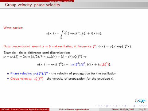
Linear transport equation
Group velocity, phase velocity
Wave packet:
u(x , t) =
∫R
φ(ξ) exp(itω(ξ) + iξx) dξ.
Data concentrated around x = 0 and oscillating at frequency ξ0: φ(x) = ψ(x) exp(iξ0x).
Example - finite difference semi-discretization:ω = ωh(ξ) = 2 sin(ξh/2)/h ∼ ωh(ξ0) + (ξ − ξ0)ω′h(ξ0) ⇒
u(x , t) ∼ exp(iξ0(x + tωh(ξ0)/ξ0))ψ(x + tω′h(ξ0)).
Phase velocity: ωh(ξ0)/ξ0 - the velocity of propagation for the oscillation
Group velocity: ω′h(ξ0) - the velocity of propagation for the envelope ψ.
(BCAM - Basque Center for Applied Mathematics) Finite difference approximations Bilbao - 11-15/06/2012 19 / 21

Linear transport equation
Geometric Optics
Light has a dual nature: is particle (photon) and is wave (and oscillates at a certain wavelength).
Geometric Optics (GO) studies the propagation of light particles along trajectories called rays.
Hamilton principle states that the trajectory of a particle between times t1 and t2 minimizes the
actiont2∫
t1
L(q, q′, t) dt, where L = T − V is the difference between kinetic and potential energies,
q is the vector of generalized coordinates and q′ = ∂t q.
Hamiltonian system associated to H = H(p, q): p′(s) = ∇qH(p(s), q(s)),q′(s) = −∇pH(p(s), q(s)).
For the continuous wave equation, H = H(x , t, ξ, τ) = τ2 − |ξ|2 and the rays of GO verify theHamiltonian system:x ′(s) = ∇ξH(x(s), t(s), ξ(s), τ(s)) = −2ξ(s), t′(s) = ∂τH(x(s), t(s), ξ(s), τ(s)) = 2τ(s)ξ′(s) = −∇x H(x(s), t(s), ξ(s), τ(s)) = 0 ⇒ ξ(s) = ξ0, τ ′(s) = −∇t H(x(s), t(s), ξ(s), τ(s)) = 0⇒ τ(s) = τ0.
Null-bi-characteristics. H(x(0), t(0), ξ(0), τ(0)) = 0. Then H(x(s), t(s), ξ(s), τ(s)) = 0 ∀s > 0.
Characteristics. Replace s by t in the Hamiltonian system. Since H(x(0), 0, ξ(0), τ(0)) = 0 hastwo roots as equation in τ0, τ0 = ±|ξ0|, then x ′(t) = ±ξ0/|ξ0| ⇒ two characteristics:x(t) = x0 ± tξ0/|ξ0|. They propagate at unit velocity.
For the finite difference semi-discretization of the wave equation, the Hamiltonian isH(x , t, ξ, τ) = τ2 − 4 sin2(ξh)/h2 and the characteristics propagate with the group velocity, i.e.x(t) = x0 ± t cos(ξ0h/2) (exercise).
(BCAM - Basque Center for Applied Mathematics) Finite difference approximations Bilbao - 11-15/06/2012 20 / 21

Linear transport equation
Some related bibliography
T.-C. Poon, Engineering Optics With Matlab, World Scientific, 2004.
A. Quarteroni, A. Valli, Numerical approximation of PDEs, Springer, 2008.
J.C. Strikwerda, Finite difference schemes and PDEs, SIAM, 2004.
L.N. Trefethen, Group velocity ub finite difference schemes, SIAM Rev. 1982.
L.N. Trefethen, Spectral methods in Matlab, SIAM, 2000.
L.N. Trefethen, Finite difference and spectral methods for ordinary and PDEs, 1996.
R. Vichnevetsky, B. Bowles, Fourier analysis of numerical approximations of hyperbolicequations, SIAM, 1982.
E. Zuazua, Metodos numericos de resolucion de Ecuaciones en Derivadas Parciales,chapters 3 and 9.
(BCAM - Basque Center for Applied Mathematics) Finite difference approximations Bilbao - 11-15/06/2012 21 / 21